Soil Classification (AASHTO and USCS)
Soil Classification (AASHTO and USCS)
Soil Classification (AASHTO and USCS)

You also want an ePaper? Increase the reach of your titles
YUMPU automatically turns print PDFs into web optimized ePapers that Google loves.
CE 240<br />
<strong>Soil</strong> Mechanics & Foundations<br />
Lecture 3.2<br />
Engineering <strong>Classification</strong> of <strong>Soil</strong><br />
(<strong>AASHTO</strong> <strong>and</strong> <strong>USCS</strong>)<br />
(Das, Ch. 4)
Outline of this Lecture<br />
1. Particle distribution <strong>and</strong> Atterberg Limits<br />
2. <strong>Soil</strong> classification systems based on<br />
particle distribution <strong>and</strong> Atterberg Limits<br />
3. American Association of State Highway <strong>and</strong><br />
Transportation Officials System (<strong>AASHTO</strong>)<br />
4. The Unified <strong>Soil</strong> <strong>Classification</strong> System<br />
(<strong>USCS</strong>)
Objective<br />
Classifying soils into groups with similar<br />
behavior, in terms of simple indices, can<br />
provide geotechnical engineers a general<br />
guidance about engineering properties of the<br />
soils through the accumulated experience.<br />
Simple indices<br />
GSD, LL, PI<br />
Communicate<br />
between<br />
engineers<br />
<strong>Classification</strong><br />
system<br />
(Language)<br />
Use the<br />
accumulated<br />
experience<br />
Estimate<br />
engineering<br />
properties<br />
Achieve<br />
engineering<br />
purposes
<strong>Classification</strong> Systems<br />
• Two commonly used systems for soil<br />
engineers based on particle distribution<br />
<strong>and</strong> Atterberg limits:<br />
• American Association of State Highway<br />
<strong>and</strong> Transportation Officials (<strong>AASHTO</strong>)<br />
System (for state/county highway dept.)<br />
• Unified <strong>Soil</strong> <strong>Classification</strong> System (<strong>USCS</strong>)<br />
(preferred by geotechnical engineers).
<strong>Soil</strong> particles<br />
The description of the grain size distribution of soil<br />
particles according to their texture (particle size,<br />
shape, <strong>and</strong> gradation).<br />
Major textural classes include, very roughly:<br />
gravel (>2 mm);<br />
s<strong>and</strong> (0.1 – 2 mm);<br />
silt (0.01 – 0.1 mm);<br />
clay (< 0.01 mm).<br />
Furthermore, gravel <strong>and</strong> s<strong>and</strong> can be roughly<br />
classified as coarse textured soils, wile silt <strong>and</strong> clay<br />
can be classified as fine textures soils.
Cobbles or Boulders<br />
Grain Size Distribution Curves<br />
GRAVEL SAND FINES
Atterberg limits<br />
Atterberg limits are the limits of water content used to<br />
define soil behavior. The consistency of soils according<br />
to Atterberg limits gives the following diagram.
American Association of State<br />
Highway <strong>and</strong> Transportation<br />
Officials system (<strong>AASHTO</strong>)<br />
Origin of <strong>AASHTO</strong>: (For road construction)<br />
This system was originally developed by<br />
Hogentogler <strong>and</strong> Terzaghi in 1929 as the Public<br />
Roads <strong>Classification</strong> System. Afterwards, there are<br />
several revisions. The present <strong>AASHTO</strong> (1978)<br />
system is primarily based on the version in 1945.<br />
(Holtz <strong>and</strong> Kovacs, 1981)
Definition of Grain Size<br />
No specific grain<br />
size-use<br />
Atterberg limits<br />
Boulders Silt-Clay<br />
Gravel S<strong>and</strong><br />
75 mm<br />
No.4<br />
4.75 mm<br />
Coarse Fine<br />
No.40<br />
0.425 mm<br />
No.200<br />
0.075<br />
mm
<strong>Classification</strong><br />
(Proceeding from left to right against the columns)<br />
Das, Table 4.1, 2006
Note:<br />
<strong>Classification</strong> (Cont.)<br />
The first group from the left to fit the test data is the<br />
correct <strong>AASHTO</strong> classification.<br />
Das, Table 4.1, 2006
Group Index GI<br />
200<br />
200<br />
[ ]<br />
GI = ( F − 35) 0.2 + 0.005( LL −40)<br />
+ 0.01( F −15)( PI −10)<br />
(4.1)<br />
For Group A-2-6 <strong>and</strong> A-2-7<br />
200<br />
The first term is determined by the LL<br />
The second term is determined by the PI<br />
GI = 0.01( F −15)( PI −10) (4.2) use the second term only<br />
F200: percentage passing through the No.200 sieve<br />
In general, the rating for a pavement subgrade is<br />
inversely proportional to the group index, GI.
Some Explanations of Group Index GI<br />
1, if Eq. 4.1 gives a negative value then GI=0;<br />
2, round up the value calculated by Eq. 4.1 to<br />
an integer;<br />
3, there is no upper limit for GI;<br />
4, the GIs for soil groups A-1-a, A-1-b, A-2-4,<br />
A-2-5, <strong>and</strong> A-3 are always zero (0).
(PI)<br />
(LL)<br />
Das, Figure 4.1
General Guidance<br />
– 8 major groups: A1~ A7 (with several subgroups) <strong>and</strong><br />
organic soils A8<br />
– The required tests are sieve analysis <strong>and</strong> Atterberg<br />
limits.<br />
– The group index, an empirical formula, is used to<br />
further evaluate soils within a group (subgroups).<br />
A1 ~ A3<br />
Granular Materials<br />
≤ 35% pass No. 200 sieve<br />
Using LL <strong>and</strong> PI separates silty<br />
materials from clayey materials (only<br />
for A2 group)<br />
A4 ~ A7<br />
Silt-clay Materials<br />
≥ 36% pass No. 200 sieve<br />
Using LL <strong>and</strong> PI separates silty<br />
materials from clayey materials<br />
– The original purpose of this classification system is<br />
used for road construction (subgrade rating).
Example 4.1, <strong>Soil</strong> B<br />
Passing No.200 86%<br />
LL=70, PI=32<br />
LL-30=40 > PI=32<br />
GI<br />
= ( F<br />
200<br />
+ 0.<br />
01(<br />
F<br />
=<br />
33.<br />
47<br />
− 35)<br />
200<br />
≅<br />
33<br />
[ 0.<br />
2 + 0.<br />
005(<br />
LL − 40)<br />
]<br />
−15)(<br />
PI −10)<br />
Round off<br />
A-7-5(33)
This is the example<br />
of Das, Example 4.1<br />
for the <strong>AASHTO</strong><br />
system classification
<strong>USCS</strong> <strong>Classification</strong> System<br />
• Originally developed for the United<br />
States Army Corps of Engineers<br />
(USACE)<br />
• The method is st<strong>and</strong>ardized in ASTM D<br />
2487 as “Unified <strong>Soil</strong> <strong>Classification</strong><br />
System (<strong>USCS</strong>)”<br />
• <strong>USCS</strong> is the most common soil<br />
classification system among<br />
geotechnical engineers
Unified <strong>Soil</strong> <strong>Classification</strong> System<br />
Origin of <strong>USCS</strong>:<br />
(<strong>USCS</strong>)<br />
This system was first developed by Professor A.<br />
Casagr<strong>and</strong>e (1948) for the purpose of airfield<br />
construction during World War II. Afterwards, it was<br />
modified by Professor Casagr<strong>and</strong>e, the U.S. Bureau of<br />
Reclamation, <strong>and</strong> the U.S. Army Corps of Engineers to<br />
enable the system to be applicable to dams,<br />
foundations, <strong>and</strong> other construction.<br />
Four major divisions:<br />
(1) Coarse-grained<br />
(2) Fine-grained<br />
(3) Organic soils<br />
(4) Peat
Boulders<br />
Definition of Grain Size<br />
Cobbles<br />
300 mm<br />
75 mm<br />
Gravel S<strong>and</strong><br />
Coarse Fine Coarse Medium Fine<br />
No.4<br />
4.75 mm<br />
19 mm No.10 No.40<br />
2.0 mm<br />
No specific grain sizeuse<br />
Atterberg limits<br />
0.425 mm<br />
No.200<br />
0.075<br />
mm<br />
Silt <strong>and</strong><br />
Clay
(Das, Table 4.2)
• <strong>Soil</strong> symbols:<br />
• G: Gravel<br />
• S: S<strong>and</strong><br />
• M: Silt<br />
• C: Clay<br />
• O: Organic<br />
• Pt: Peat<br />
Example: SW, Well-graded s<strong>and</strong><br />
SC, Clayey s<strong>and</strong><br />
SM, Silty s<strong>and</strong>,<br />
MH, Elastic silt<br />
The Symbols<br />
• Liquid limit<br />
symbols:<br />
• H: High LL (LL>50)<br />
• L: Low LL (LL
<strong>USCS</strong> System (cont.)<br />
• A typical <strong>USCS</strong> classification would be:<br />
Group<br />
Symbol<br />
-<br />
SM Silty s<strong>and</strong> with gravel<br />
Group<br />
Name
<strong>Classification</strong> of <strong>Soil</strong>s<br />
• From sieve analysis <strong>and</strong> the grain-size<br />
distribution curve determine the percent<br />
passing as the following:<br />
– > 3 inch – Cobble or Boulders<br />
– 3 inch - # 4 (76.2 – 4.75 mm) : Gravel<br />
– # 4 - # 200 (4.75 - 0.075 mm) : S<strong>and</strong><br />
– < # 200: Fines<br />
• First, Find % passing # 200<br />
• If 5% or more of the soil passes the # 200<br />
sieve, then conduct Atterberg Limits (LL &<br />
PL)
<strong>Classification</strong> of <strong>Soil</strong>s<br />
• If the soil is fine-grained (≥ 50% passes<br />
#200) follow the guidelines for fine-grained<br />
soils<br />
• If the soil is coarse-grained (
50%<br />
General Guidance<br />
Coarse-grained soils:<br />
Gravel S<strong>and</strong><br />
•Grain size distribution<br />
•C u<br />
•C c<br />
NO. 4<br />
4.75 mm<br />
50 %<br />
NO.200<br />
0.075 mm<br />
Required tests: Sieve analysis<br />
Fine-grained soils:<br />
Silt Clay<br />
Atterberg limit<br />
•PL, LL<br />
•Plasticity chart<br />
LL>50<br />
LL
Coarse-grained <strong>Soil</strong>s
Fine-grained <strong>Soil</strong>s
Gravel<br />
98-62 = 36%<br />
S<strong>and</strong><br />
62-8 = 54%<br />
Fines = 8%<br />
Example – <strong>Soil</strong> A<br />
gravel s<strong>and</strong> fines<br />
<strong>Soil</strong> A: D 60 = 4.2 mm , D 30 = 0.6 mm, D 10 = 0.09 mm<br />
Cu = 46.67<br />
Cc = 0.95
Grave = 36%<br />
S<strong>and</strong> = 54%<br />
Fines = 8%<br />
Cu = 46.7<br />
Cc = 0.95<br />
LL = 42<br />
PL = 31<br />
PI = 42-31 = 11<br />
GO TO Plasticity<br />
Chart<br />
Example – <strong>Soil</strong> A (Cont.)
Example – <strong>Soil</strong> A (Cont.)<br />
• <strong>Soil</strong> A is then classified as<br />
SP-SM – Poorly-grades s<strong>and</strong> with silt <strong>and</strong><br />
gravel
LL = 42<br />
PL = 31<br />
PI = 42-31 = 11<br />
Example – <strong>Soil</strong> A (Cont.)<br />
ML
PI<br />
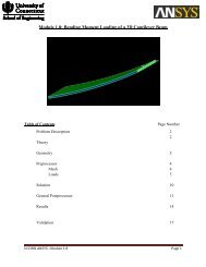
The Plasticity Chart<br />
L<br />
H<br />
LL<br />
(Holtz <strong>and</strong> Kovacs, 1981)<br />
• The A-line generally<br />
separates the more<br />
claylike materials<br />
from silty materials,<br />
<strong>and</strong> the organics<br />
from the inorganics.<br />
• The U-line indicates<br />
the upper bound for<br />
general soils.<br />
Note: If the measured<br />
limits of soils are on<br />
the left of U-line,<br />
they should be<br />
rechecked.
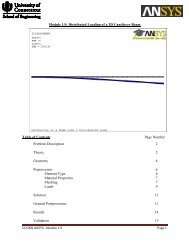
Procedures for <strong>Classification</strong><br />
Coarse-grained<br />
material<br />
Grain size<br />
distribution<br />
Fine-grained<br />
material<br />
LL, PI<br />
Highly<br />
(Santamarina et al., 2001)
Example<br />
Passing No.200 sieve 30 %<br />
Passing No.4 sieve 70 %<br />
LL= 33<br />
PI= 12<br />
PI= 0.73(LL-20), A-line<br />
PI=0.73(33-20)=9.49<br />
SC<br />
(≥15% gravel)<br />
Clayey s<strong>and</strong> with<br />
gravel<br />
Passing No.200 sieve 30 %<br />
Passing No.4 sieve 70 %<br />
Highly<br />
LL= 33<br />
PI= 12<br />
(Santamarina et al., 2001)
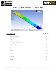
Organic <strong>Soil</strong>s<br />
Highly organic soils- Peat (Group symbol PT)<br />
− A sample composed primarily of vegetable tissue in<br />
various stages of decomposition <strong>and</strong> has a fibrous to<br />
amorphous texture, a dark-brown to black color, <strong>and</strong> an<br />
organic odor should be designated as a highly organic<br />
soil <strong>and</strong> shall be classified as peat, PT.<br />
Organic clay or silt( group symbol OL or OH):<br />
− “The soil’s liquid limit (LL) after oven drying is less than<br />
75 % of its liquid limit before oven drying.” If the above<br />
statement is true, then the first symbol is O.<br />
− The second symbol is obtained by locating the values<br />
of PI <strong>and</strong> LL (not oven dried) in the plasticity chart.
This is the Figure 4.7 of Das’ textbook, the scanning<br />
electron micrographs (SEM) for 4 peat samples.
Borderline Cases (Dual Symbols)<br />
For the following three conditions, a dual<br />
symbol should be used.<br />
–Coarse-grained soils with 5% - 12% fines.<br />
−About 7 % fines can change the hydraulic<br />
conductivity of the coarse-grained media by<br />
orders of magnitude.<br />
−The first symbol indicates whether the coarse<br />
fraction is well or poorly graded. The second<br />
symbol describe the contained fines. For example:<br />
SP-SM, poorly graded s<strong>and</strong> with silt.
Borderline Cases (Dual Symbols, cont.)<br />
–Fine-grained soils with limits within the<br />
shaded zone. (PI between 4 <strong>and</strong> 7 <strong>and</strong> LL<br />
between about 12 <strong>and</strong> 25).<br />
−It is hard to distinguish between the silty <strong>and</strong> more<br />
claylike materials.<br />
−CL-ML: Silty clay, SC-SM: Silty, clayed s<strong>and</strong>.<br />
–<strong>Soil</strong> contain similar fines <strong>and</strong> coarse-grained<br />
fractions.<br />
− possible dual symbols GM-ML
Borderline Cases (Summary)<br />
(Holtz <strong>and</strong> Kovacs, 1981)
Reading Assignment:<br />
Das, Ch. 4<br />
Homework:<br />
Problem 4.3