LDPC Codes – a brief Tutorial

More documents

Recommendations

Info

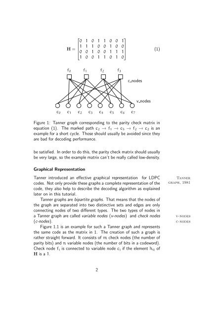
⎡ 0 ⎢ H = ⎢1 ⎣0 1 1 0 0 1 1 1 0 0 1 0 0 0 1 1 0 0 1 ⎤ 1 0 ⎥ 1⎦ 1 0 0 1 1 0 1 0 f0 f1 c0 c1 c2 c3 c4 c5 c6 c7 f2 f3 c nodes v nodes Figure 1: Tanner graph corresponding to the parity check matrix in equation (1). The marked path c2 → f1 → c5 → f2 → c2 is an example for a short cycle. Those should usually be avoided since they are bad for decoding performance. be satisfied. In order to do this, the parity check matrix should usually be very large, so the example matrix can’t be really called low-density. Graphical Representation Tanner introduced an effective graphical representation for LDPC Tanner graph, 1981 codes. Not only provide these graphs a complete representation of the code, they also help to describe the decoding algorithm as explained later on in this tutorial. Tanner graphs are bipartite graphs. That means that the nodes of the graph are separated into two distinctive sets and edges are only connecting nodes of two different types. The two types of nodes in a Tanner graph are called variable nodes (v-nodes) and check nodes v-nodes (c-nodes). c-nodes Figure 1.1 is an example for such a Tanner graph and represents the same code as the matrix in 1. The creation of such a graph is rather straight forward. It consists of m check nodes (the number of parity bits) and n variable nodes (the number of bits in a codeword). Check node fi is connected to variable node cj if the element hij of H is a 1. 2 (1)
1.2 Regular and irregular LDPC codes A LDPC code is called regular if wc is constant for every column regular and wr = wc · (n/m) is also constant for every row. The example matrix from equation (1) is regular with wc = 2 and wr = 4. It’s also possible to see the regularity of this code while looking at the graphical representation. There is the same number of incoming edges for every v-node and also for all the c-nodes. If H is low density but the numbers of 1’s in each row or column aren’t constant the code is called a irregular LDPC code. irregular 1.3 Constructing LDPC codes Several different algorithms exists to construct suitable LDPC codes. Gallager himself introduced one. Furthermore MacKay proposed one MacKay to semi-randomly generate sparse parity check matrices. This is quite interesting since it indicates that constructing good performing LDPC codes is not a hard problem. In fact, completely randomly chosen codes are good with a high probability. The problem that will arise, is that the encoding complexity of such codes is usually rather high. 2 Performance & Complexity Before describing decoding algorithms in section 3, I would like to explain why all this effort is needed. The feature of LDPC codes to perform near the Shannon limit 1 of a channel exists only for large block lengths. For example there have been simulations that perform within 0.04 dB of the Shannon limit at a bit error rate of 10 −6 with an Shannon limit block length of 10 7 . An interesting fact is that those high performance codes are irregular. The large block length results also in large parity-check and generator matrices. The complexity of multiplying a codeword with a matrix depends on the amount of 1’s in the matrix. If we put the sparse matrix H in the form [P T I] via Gaussian elimination the generator matrix G can be calculated as G = [I P]. The sub-matrix P is generally not sparse so that the encoding complexity will be quite high. 1 Shannon proofed that reliable communication over an unreliable channel is only possible with code rates above a certain limit – the channel capacity. 3
Page 1: LDPC Codes - a brief Tutorial Bernh
Page 5 and 6: c-node received/sent f0 received: c
Page 7 and 8: a) b) qij(b) fj ci rji(b) qij(b) fj
Page 9: of the message bits and some parity

LDPC Codes – a brief Tutorial

You also want an ePaper? Increase the reach of your titles

Delete template?

Save as template?