
Create successful ePaper yourself
Turn your PDF publications into a flip-book with our unique Google optimized e-Paper software.
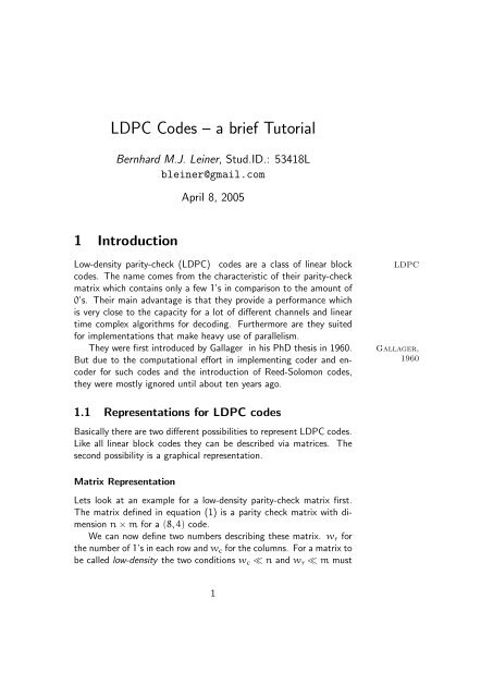
<strong>LDPC</strong> <strong>Codes</strong> <strong>–</strong> a <strong>brief</strong> <strong>Tutorial</strong><br />
Bernhard M.J. Leiner, Stud.ID.: 53418L<br />
bleiner@gmail.com<br />
1 Introduction<br />
April 8, 2005<br />
Low-density parity-check (<strong>LDPC</strong>) codes are a class of linear block <strong>LDPC</strong><br />
codes. The name comes from the characteristic of their parity-check<br />
matrix which contains only a few 1’s in comparison to the amount of<br />
0’s. Their main advantage is that they provide a performance which<br />
is very close to the capacity for a lot of different channels and linear<br />
time complex algorithms for decoding. Furthermore are they suited<br />
for implementations that make heavy use of parallelism.<br />
They were first introduced by Gallager in his PhD thesis in 1960. Gallager,<br />
But due to the computational effort in implementing coder and encoder<br />
for such codes and the introduction of Reed-Solomon codes,<br />
they were mostly ignored until about ten years ago.<br />
1960<br />
1.1 Representations for <strong>LDPC</strong> codes<br />
Basically there are two different possibilities to represent <strong>LDPC</strong> codes.<br />
Like all linear block codes they can be described via matrices. The<br />
second possibility is a graphical representation.<br />
Matrix Representation<br />
Lets look at an example for a low-density parity-check matrix first.<br />
The matrix defined in equation (1) is a parity check matrix with dimension<br />
n × m for a (8, 4) code.<br />
We can now define two numbers describing these matrix. wr for<br />
the number of 1’s in each row and wc for the columns. For a matrix to<br />
be called low-density the two conditions wc ≪ n and wr ≪ m must<br />
1
⎡<br />
0<br />
⎢<br />
H = ⎢1<br />
⎣0<br />
1<br />
1<br />
0<br />
0<br />
1<br />
1<br />
1<br />
0<br />
0<br />
1<br />
0<br />
0<br />
0<br />
1<br />
1<br />
0<br />
0<br />
1<br />
⎤<br />
1<br />
0 ⎥<br />
1⎦<br />
1 0 0 1 1 0 1 0<br />
f0<br />
f1<br />
c0 c1 c2 c3 c4 c5 c6 c7<br />
f2<br />
f3<br />
c nodes<br />
v nodes<br />
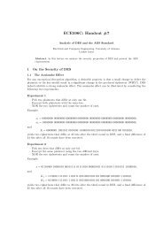
Figure 1: Tanner graph corresponding to the parity check matrix in<br />
equation (1). The marked path c2 → f1 → c5 → f2 → c2 is an<br />
example for a short cycle. Those should usually be avoided since they<br />
are bad for decoding performance.<br />
be satisfied. In order to do this, the parity check matrix should usually<br />
be very large, so the example matrix can’t be really called low-density.<br />
Graphical Representation<br />
Tanner introduced an effective graphical representation for <strong>LDPC</strong> Tanner<br />
graph, 1981<br />
codes. Not only provide these graphs a complete representation of the<br />
code, they also help to describe the decoding algorithm as explained<br />
later on in this tutorial.<br />
Tanner graphs are bipartite graphs. That means that the nodes of<br />
the graph are separated into two distinctive sets and edges are only<br />
connecting nodes of two different types. The two types of nodes in<br />
a Tanner graph are called variable nodes (v-nodes) and check nodes v-nodes<br />
(c-nodes). c-nodes<br />
Figure 1.1 is an example for such a Tanner graph and represents<br />
the same code as the matrix in 1. The creation of such a graph is<br />
rather straight forward. It consists of m check nodes (the number of<br />
parity bits) and n variable nodes (the number of bits in a codeword).<br />
Check node fi is connected to variable node cj if the element hij of<br />
H is a 1.<br />
2<br />
(1)
1.2 Regular and irregular <strong>LDPC</strong> codes<br />
A <strong>LDPC</strong> code is called regular if wc is constant for every column regular<br />
and wr = wc · (n/m) is also constant for every row. The example<br />
matrix from equation (1) is regular with wc = 2 and wr = 4. It’s also<br />
possible to see the regularity of this code while looking at the graphical<br />
representation. There is the same number of incoming edges for every<br />
v-node and also for all the c-nodes.<br />
If H is low density but the numbers of 1’s in each row or column<br />
aren’t constant the code is called a irregular <strong>LDPC</strong> code. irregular<br />
1.3 Constructing <strong>LDPC</strong> codes<br />
Several different algorithms exists to construct suitable <strong>LDPC</strong> codes.<br />
Gallager himself introduced one. Furthermore MacKay proposed one MacKay<br />
to semi-randomly generate sparse parity check matrices. This is quite<br />
interesting since it indicates that constructing good performing <strong>LDPC</strong><br />
codes is not a hard problem. In fact, completely randomly chosen<br />
codes are good with a high probability. The problem that will arise,<br />
is that the encoding complexity of such codes is usually rather high.<br />
2 Performance & Complexity<br />
Before describing decoding algorithms in section 3, I would like to<br />
explain why all this effort is needed. The feature of <strong>LDPC</strong> codes to<br />
perform near the Shannon limit 1 of a channel exists only for large<br />
block lengths. For example there have been simulations that perform<br />
within 0.04 dB of the Shannon limit at a bit error rate of 10 −6 with an Shannon limit<br />
block length of 10 7 . An interesting fact is that those high performance<br />
codes are irregular.<br />
The large block length results also in large parity-check and generator<br />
matrices. The complexity of multiplying a codeword with a<br />
matrix depends on the amount of 1’s in the matrix. If we put the<br />
sparse matrix H in the form [P T I] via Gaussian elimination the generator<br />
matrix G can be calculated as G = [I P]. The sub-matrix P<br />
is generally not sparse so that the encoding complexity will be quite<br />
high.<br />
1 Shannon proofed that reliable communication over an unreliable channel is<br />
only possible with code rates above a certain limit <strong>–</strong> the channel capacity.<br />
3
Since the complexity grows in O(n2 ) even sparse matrices don’t<br />
result in a good performance if the block length gets very high. So iterative<br />
decoding (and encoding) algorithms are used. Those algorithms<br />
perform local calculations and pass those local results via messages.<br />
This step is typically repeated several times.<br />
The term ”local calculations” already indicates that a divide and<br />
conquere strategy, which separates a complex problem into manage- divide and<br />
able sub-problems, is realized. A sparse parity check matrix now helps conquere<br />
this algorithms in several ways. First it helps to keep both the local<br />
calculations simple and also reduces the complexity of combining<br />
the sub-problems by reducing the number of needed messages to exchange<br />
all the information. Furthermore it was observed that iterative<br />
decoding algorithms of sparse codes perform very close to the optimal<br />
maximum likelihood decoder.<br />
3 Decoding <strong>LDPC</strong> codes<br />
The algorithm used to decode <strong>LDPC</strong> codes was discovered independently<br />
several times and as a matter of fact comes under different<br />
names. The most common ones are the belief propagation algorithm<br />
, the message passing algorithm and the sum-product algorithm. BPA<br />
In order to explain this algorithm, a very simple variant which works<br />
with hard decision, will be introduced first. Later on the algorithm will<br />
be extended to work with soft decision which generally leads to better<br />
decoding results. Only binary symmetric channels will be considered.<br />
3.1 Hard-decision decoding<br />
The algorithm will be explained on the basis of the example code<br />
already introduced in equation 1 and figure 1.1. An error free received<br />
codeword would be e.g. c = [1 0 0 1 0 1 0 1]. Let’s suppose that we<br />
have a BHC channel and the received the codeword with one error <strong>–</strong><br />
bit c1 flipped to 1.<br />
MPA<br />
SPA<br />
1. In the first step all v-nodes ci send a ”message” to their (always ci → fj<br />
2 in our example) c-nodes fj containing the bit they believe to<br />
be the correct one for them. At this stage the only information<br />
a v-node ci has, is the corresponding received i-th bit of c, yi.<br />
That means for example, that c0 sends a message containing 1<br />
to f1 and f3, node c1 sends messages containing y1 (1) to f0<br />
and f1, and so on.<br />
4
c-node received/sent<br />
f0 received: c1 → 1 c3 → 1 c4 → 0 c7 → 1<br />
sent: 0 → c1 0 → c3 1 → c4 0 → c7<br />
f1 received: c0 → 1 c1 → 1 c2 → 0 c5 → 1<br />
sent: 0 → c0 0 → c1 1 → c2 0 → c5<br />
f2 received: c2 → 0 c5 → 1 c6 → 0 c7 → 1<br />
sent: 0 → c2 1 → c5 0 → c6 1 → c7<br />
f3 received: c0 → 1 c3 → 1 c4 → 0 c6 → 0<br />
sent: 1 → c0 1 → c3 0 → c4 0 → c6<br />
Table 1: overview over messages received and sent by the c-nodes in<br />
step 2 of the message passing algorithm<br />
2. In the second step every check nodes fj calculate a response to fj → ci<br />
every connected variable node. The response message contains<br />
the bit that fj believes to be the correct one for this v-node ci<br />
assuming that the other v-nodes connected to fj are correct.<br />
In other words: If you look at the example, every c-node fj is<br />
connected to 4 v-nodes. So a c-node fj looks at the message received<br />
from three v-nodes and calculates the bit that the fourth<br />
v-node should have in order to fulfill the parity check equation.<br />
Table 2 gives an overview about this step.<br />
Important is, that this might also be the point at which the decoding<br />
algorithm terminates. This will be the case if all check<br />
equations are fulfilled. We will later see that the whole algorithm<br />
contains a loop, so an other possibility to stop would be<br />
a threshold for the amount of loops.<br />
3. Next phase: the v-nodes receive the messages from the check ci → fj<br />
nodes and use this additional information to decide if their originally<br />
received bit is OK. A simple way to do this is a majority<br />
vote. When coming back to our example that means, that each<br />
v-node has three sources of information concerning its bit. The<br />
original bit received and two suggestions from the check nodes.<br />
Table 3 illustrates this step. Now the v-nodes can send another<br />
message with their (hard) decision for the correct value to the<br />
check nodes.<br />
4. Go to step 2. loop<br />
In our example, the second execution of step 2 would terminate the<br />
decoding process since c1 has voted for 0 in the last step. This corrects<br />
5
v-node yi received messages from check nodes decision<br />
c0 1 f1 → 0 f3 → 1 1<br />
c1 1 f0 → 0 f1 → 0 0<br />
c2 0 f1 → 1 f2 → 0 0<br />
c3 1 f0 → 0 f3 → 1 1<br />
c4 0 f0 → 1 f3 → 0 0<br />
c5 1 f1 → 0 f2 → 1 1<br />
c6 0 f2 → 0 f3 → 0 0<br />
c7 1 f0 → 1 f2 → 1 1<br />
Table 2: Step 3 of the described decoding algorithm. The v-nodes<br />
use the answer messages from the c-nodes to perform a majority vote<br />
on the bit value.<br />
the transmission error and all check equations are now satisfied.<br />
3.2 Soft-decision decoding<br />
The above description of hard-decision decoding was mainly for educational<br />
purpose to get an overview about the idea. Soft-decision<br />
decoding of <strong>LDPC</strong> codes, which is based on the concept of belief<br />
propagation, yields in a better decoding performance and is therefore belief<br />
the prefered method. The underlying idea is exactly the same as in propagation<br />
hard decision decoding. Before presenting the algorithm lets introduce<br />
some notations:<br />
• Pi = Pr(ci = 1|yi)<br />
• qij is a message sent by the variable node ci to the check node<br />
fj. Every message contains always the pair qij(0) and qij(1)<br />
which stands for the amount of belief that yi is a ”0” or a ”1”.<br />
• rji is a message sent by the check node fj to the variable node<br />
ci. Again there is a rji(0) and rji(1) that indicates the (current)<br />
amount of believe in that yi is a ”0” or a ”1”.<br />
The step numbers in the following description correspond to the<br />
hard decision case.<br />
1. All variable nodes send their qij messages. Since no other ci → fj<br />
information is avaiable at this step, qij(1) = Pi and qij(0) =<br />
1 − Pi.<br />
6
a) b)<br />
qij(b)<br />
fj<br />
ci<br />
rji(b)<br />
qij(b)<br />
fj<br />
ci<br />
yi<br />
rji(b)<br />
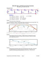
Figure 2: a) illustrates the calculation of rji(b) and b) qij(b)<br />
2. The check nodes calculate their response messages rji: 2<br />
and<br />
rji(0) = 1 1<br />
+<br />
2 2<br />
�<br />
i ′ ɛ Vj\i<br />
(1 − 2qi ′ j(1)) (3)<br />
rji(1) = 1 − rji(0) (4)<br />
So they calculate the probability that there is an even number<br />
of 1’s amoung the variable nodes except ci (this is exactly what<br />
Vj\i means). This propability is equal to the probability rji(0)<br />
that ci is a 0. This step and the information used to calculate<br />
the responses is illustrated in figure 2.<br />
fj → ci<br />
3. The variable nodes update their response messages to the check<br />
nodes. This is done according to the following equations,<br />
ci → fj<br />
qij(0) = Kij (1 − Pi) �<br />
rj ′ i(0) (5)<br />
qij(1) = KijPi<br />
�<br />
j ′ ɛ Ci\j<br />
j ′ ɛ Ci\j<br />
rj ′ i(1) (6)<br />
2 Equation 3 uses the following result from Gallager: for a sequence of M<br />
independent binary digits ai with an propability of pi for ai = 1, the probability<br />
that the whole sequence contains an even number of 1’s is<br />
1 1<br />
+<br />
2 2<br />
M�<br />
(1 − 2pi) (2)<br />
i=1<br />
7
whereby the Konstants Kij are chosen in a way to ensure that<br />
qij(0) + qij(1) = 1. Ci\j now means all check nodes except fj.<br />
Again figure 2 illustrates the calculation in this step.<br />
At this point the v-nodes also update their current estimation ^ci<br />
of their variable ci. This is done by calculating the propabilities<br />
for 0 and 1 and voting for the bigger one. The used equations<br />
Qi(0) = Ki (1 − Pi) �<br />
rji(0) (7)<br />
and<br />
j ɛ Ci<br />
�<br />
Qi(1) = KiPi rji(1) (8)<br />
j ɛ Ci<br />
are quite similar to the ones to compute qij(b) but now the<br />
information from every c-node is used.<br />
^ci =<br />
�<br />
1 if Qi(1) > Qi(0),<br />
0 else<br />
If the current estimated codeword fufills now the parity check<br />
equations the algorithm terminates. Otherwise termination is<br />
ensured through a maximum number of iterations.<br />
4. Go to step 2. loop<br />
The explained soft decision decoding algorithm is a very simple<br />
variant, suited for BSC channels and could be modified for performance<br />
improvements. Beside performance issues there are nummerical<br />
stability problems due to the many multiplications of probabilities.<br />
The results will come very close to zero for large block lenghts. To<br />
prevent this, it is possible to change into the log-domain and doing log-domain<br />
additions instead of multiplications. The result is a more stable algorithm<br />
that even has performance advantages since additions are less<br />
costly.<br />
4 Encoding<br />
The sharped eyed reader will have noticed that the above decoding<br />
algorithm does in fact only error correction. This would be enough for<br />
a traditional systematic block code since the code word would consist<br />
8<br />
(9)
of the message bits and some parity check bits. So far nowhere was<br />
mentioned that it’s possible to directly see the original message bits<br />
in a <strong>LDPC</strong> encoded message. Luckily it is.<br />
Encoding <strong>LDPC</strong> codes is roughly done like that: Choose certain<br />
variable nodes to place the message bits on. And in the second step<br />
calculate the missing values of the other nodes. An obvious solution<br />
for that would be to solve the parity check equations. This would<br />
contain operations involving the whole parity-check matrix and the<br />
complexity would be again quadratic in the block length. In practice<br />
however, more clever methods are used to ensure that encoding can<br />
be done in much shorter time. Those methods can use again the<br />
spareness of the parity-check matrix or dictate a certain structure 3 for<br />
the Tanner graph.<br />
5 Summary<br />
Low-density-parity-check codes have been studied a lot in the last<br />
years and huge progresses have been made in the understanding and<br />
ability to design iterative coding systems. The iterative decoding approach<br />
is already used in turbo codes but the structure of <strong>LDPC</strong> codes<br />
give even better results. In many cases they allow a higher code rate<br />
and also a lower error floor rate. Furthermore they make it possible<br />
to implement parallelizable decoders. The main disadvantes are that<br />
encoders are somehow more complex and that the code lenght has to<br />
be rather long to yield good results.<br />
For more information <strong>–</strong> and there are a lot of things which haven’t<br />
been mentioned in this tutorial <strong>–</strong> I can recommend the following web<br />
sites as a start:<br />
http://www.csee.wvu.edu/wcrl/ldpc.htm<br />
A collection of links to sites about <strong>LDPC</strong> codes and a list of<br />
papers about the topic.<br />
http://www.inference.phy.cam.ac.uk/mackay/<strong>Codes</strong>Files.html<br />
The homepage of MacKay. Very intersting are the Pictorial<br />
demonstration of iterative decoding<br />
3 It was already mentioned in section 1.3 that randomly generated <strong>LDPC</strong> codes<br />
results in high encoding complexity.<br />
9