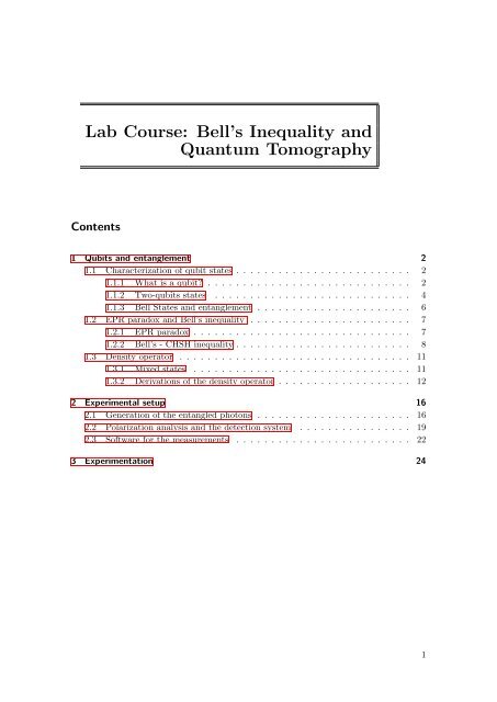
Lab Course: Bell's Inequality and Quantum Tomography

Lab Course: Bell’s Inequality and
Quantum Tomography
Contents
1 Qubits and entanglement 2
1.1 Characterization of qubit states . . . . . . . . . . . . . . . . . . . . . . . . . 2
1.1.1 What is a qubit? . . . . . . . . . . . . . . . . . . . . . . . . . . . . . 2
1.1.2 Two-qubits states . . . . . . . . . . . . . . . . . . . . . . . . . . . . 4
1.1.3 Bell States and entanglement . . . . . . . . . . . . . . . . . . . . . . 6
1.2 EPR paradox and Bell’s inequality . . . . . . . . . . . . . . . . . . . . . . . 7
1.2.1 EPR paradox . . . . . . . . . . . . . . . . . . . . . . . . . . . . . . . 7
1.2.2 Bell’s - CHSH inequality . . . . . . . . . . . . . . . . . . . . . . . . . 8
1.3 Density operator . . . . . . . . . . . . . . . . . . . . . . . . . . . . . . . . . 11
1.3.1 Mixed states . . . . . . . . . . . . . . . . . . . . . . . . . . . . . . . 11
1.3.2 Derivations of the density operator . . . . . . . . . . . . . . . . . . . 12
2 Experimental setup 16
2.1 Generation of the entangled photons . . . . . . . . . . . . . . . . . . . . . . 16
2.2 Polarization analysis and the detection system . . . . . . . . . . . . . . . . 19
2.3 Software for the measurements . . . . . . . . . . . . . . . . . . . . . . . . . 22
3 Experimentation 24
1

1 Qubits and entanglement
Bell’s Inequality &
Quantum Tomography
Advanced Laboratory Course
Entanglement lies at the heart of quantum information processing and leads to many
interesting fields of research. On the one hand it is the key element for application-oriented
quantum physics like quantum cryptography, teleportation or quantum computation and
on the other hand its characteristics can be used for a fundamental test of non-classical
properties of quantum theory. During this lab course the distinctive features of twophoton
entanglement, like the violation of a Bell inequality, shall be explained and also
the entangled state will be reconstructed completely through quantum tomography.
1 Qubits and entanglement
First of all, the theoretical framework of two-photon entangled states is described. Therefore,
the basic properties of quantum mechanics are summarized briefly (for further details
see [6]) and afterwards are adapted to two-photon entanglement.
1.1 Characterization of qubit states
1.1.1 What is a qubit?
In general, a classical physical state is described by a minimal set of physical quantities
which provides full information about the considered physical system. In classical mechanics
the state of a physical system is completely described by the generalized coordinate �q
and the generalized momentum �p. By contrast in quantum mechanics a physical state is
given by a vector in an, in general, infinite-dimensional complex vector space - the Hilbert
space [17]. In our case the dimension of the Hilbert space for a single particle is reduced
to two dimensions, because we use the polarization degree of freedom of photons. In 1995
Schumacher established the word ”Qubit” for such a state as the quantum mechanical
analogue of the classical bit. Generally, a qubit is a two-level quantum state defined as
a vector of a Hilbert space. Due to the quantum superposition principle any normalized
linear combination of two states is a possible state again. Here the two orthogonal states
can be encoded in the horizontal |H〉 and vertical |V 〉 polarization. So a general qubit
state can be written as the superposition of the two basic vectors:
� �
|ψ〉 = a |H〉 + b |V 〉 �=
a
b
with |a| 2 + |b| 2 = 1 (1.1)
By ignoring a global phase and considering the normalization implicitly [23], this can
be expressed as
2
|ψθ,φ〉 = cos( θ
2 ) |H〉 + e(iφ) sin( θ
) |V 〉 with θ ∈ [0, π] , φ ∈ [0, 2π] (1.2)
2

1.1 Characterization of qubit states
Figure 1.1: Bloch sphere represents the Hilbert space of one qubit. On the three orthogonal axis
(X,Y,Z) the eigenvectors of the Pauli matrices (�σx, �σy, �σz) are situated (from [10]).
The full Hilbert space of a single qubit can be illustrated by the Bloch sphere, as seen in
figure 1.1. A pure state |ψ〉 is represented by a vector ending at the surface of the Bloch
sphere, while a mixed state lies within the sphere. |ψ〉 is reached by rotating |H〉 by an
angle θ around the Y axis and by φ around the Z axis.
In quantum mechanics a measurement is represented by observables, i.e. hermitian
operators [6]. More precisely, it is defined as the projection onto one of the eigenstates of
the observable and the measurement result is the corresponding eigenvalue. It is convenient
to choose the Pauli spin matrices �σx, �σy, �σz and the identity � as the operators acting on
the 2-dimensional Hilbert space, because their eigenvectors form an orthogonal basis on
the 2-D Hilbert space [10]. In figure 1.1 the basis of the Bloch sphere is given by the
eigenvectors of the Pauli spin matrices.
� �
0
�σx =
1
�
1
0
= |H〉 〈V | + |V 〉 〈H|
�
�σy =
0 −i
= i(|V 〉 〈H| − |H〉 〈V |)
(1.3)
�σz =
i 0
� �
1 0
0 −1
= |H〉 〈H| − |V 〉 〈V |
A measurement of a qubit can be associated to two possible eigenvalues +1 or -1 and
the corresponding eigenvectors are defined as follows:
�σx [ 1
√ 2 (|H〉 ± |V 〉)] = �σx |+/−〉 = ± |+/−〉
�σy [ 1
√ 2 (|H〉 ± i |V 〉)] = �σy |R/L〉 = ± |R/L〉
�σz |H/V 〉 = ± |H/V 〉
(1.4)
So |+/−〉 corresponds to ±45 ◦ linear and |R/L〉 to right/ left circular polarized photons.
3

1 Qubits and entanglement
A general observable �σθ,φ can be defined in terms of the Pauli operators as:
For example:
�σθ,φ = cos(φ) sin(θ) �σx + sin(φ) sin(θ) �σy + cos(θ) �σz
�σ0,0 = �σz �σ π
(1.5)
2 ,0 = �σx �σ π π
, 2 2 = �σy (1.6)
Let us now consider, that we want to measure only the |H〉 basis vector of the state
|ψθ,φ〉. Therefore, we can calculate the probability of occurrence with the expectation
value of the projector PH which is defined as follows:
And consequently a projector P ±
θ,φ is given by:
PH = |H〉 〈H| = 1
2 (� + �σz) (1.7)
〈ψθ,φ|PH|ψθ,φ〉 = cos 2 ( θ
) (1.8)
2
P ±
θ,φ = |ψθ,φ〉 〈ψθ,φ| = 1
2 (� + �σθ,φ) (1.9)
In the last step the single qubit correlation for the pure states |ψ〉 can be calculated in
a general basis setting �σθ,φ according to:
E(θ, φ) = 〈ψ|�σθ,φ|ψ〉 = 〈ψ|P + −
θ,φ − Pθ,φ |ψ〉 = p+
θ,φ − p−
θ,φ
with the probabilities of occurrence p +
θ,φ , p−
θ,φ [25].
1.1.2 Two-qubits states
(1.10)
In this experiment the spatial separation of the two qubits as another degree of freedom
allows us to distinguish them, i.e. the two qubits can be numbered. In this section we
want to describe this state theoretically: Assuming that the two qubits represent a single
system, the corresponding Hilbert space H is given by the tensor product of the two
preceding Hilbert spaces H1 and H2 spanning the vector space of each qubit [6].
H = H1 ⊗ H2
(1.11)
A basis of H can be obtained by defining the tensor product of the single qubit basis
vectors:
4
|HH〉 = |H〉 ⊗ |H〉 |HV 〉 = |H〉 ⊗ |V 〉
|V H〉 = |V 〉 ⊗ |H〉 |V V 〉 = |V 〉 ⊗ |V 〉
So the most general two-qubit state in this basis is given by [25]:
|Ψ(aHH, aHV , aV H, aV V )〉 = aHH |HH〉 + aHV |HV 〉 + aV H |V H〉 + aV V |V V 〉
with aHH, aHV , aV H, aV V ∈ �and |aHH| 2 + |aHV | 2 + |aV H| 2 + |aV V )| 2 = 1
(1.12)
(1.13)

1.1 Characterization of qubit states
States that can be expressed as a tensor product of single qubits are called separable
or product states and any superposition of these is also an element of the Hilbert space
H. But superposition states cannot be written as a tensor product of the single qubits in
general and therefore, these kind of states is called non-separable or entangled.
In order to characterize two-photon states, observables acting on the two qubit vector
space have to be described. Let � A1 and � A2 be observables acting respectively on H1 and
H2. Their tensor product � A1 ⊗ � B2 is the observable acting on H, defined by following
relation:
[ � A1 ⊗ � A2] [|ψ1〉 ⊗ |ψ2〉] = [ � A1 |ψ1〉] ⊗ [ � A2 |ψ2〉] with ψ1 ∈ H1 and ψ2 ∈ H2
(1.14)
Any of these observables can be formed by a linear combination of tensorially multiplied
Pauli matrices:
[ � A1 ⊗ � 3�
A2] = sij �σi ⊗ �σj (1.15)
i,j=0
with �σ0 = �; �σ1 = �σx; �σ2 = �σy; �σ3 = �σz; si,j ∈ �
Using this formalism of the tensor product a projector can be defined similarly to the
single qubit case. Here the PHV projector is shown:
PHV = PH ⊗ PV = 1
2 (� + �σz) ⊗ 1
2 (� − �σz) (1.16)
For example [10], the correlation of �σz ⊗ �σz and a state |Ψ(aHH, aHV , aV H, aV V )〉 is
therefore given by:
Ezz = 〈Ψ(aHH, aHV , aV H, aV V )|�σz ⊗ �σz|Ψ(aHH, aHV , aV H, aV V )〉 =
= 1
4 (〈Ψ|[� + �σz] ⊗ [� + �σz]|Ψ〉 − 〈Ψ|[� + �σz] ⊗ [� − �σz]|Ψ〉 −
− 〈Ψ|[� + �σz] ⊗ [� − �σz]|Ψ〉 + 〈Ψ|[� − �σz] ⊗ [� − �σz]|Ψ〉) =
= 〈Ψ|PH ⊗ PH|Ψ〉 − 〈Ψ|PH ⊗ PV |Ψ〉 − 〈Ψ|PV ⊗ PH|Ψ〉 + 〈Ψ|PV ⊗ PV |Ψ〉 =
= |aHH| 2 − |aHV | 2 − |aV H| 2 + |aV V | 2 = pHH − pHV − pV H + pV V
(1.17)
where pij ({ij} ∈ {H, V }) are the probabilities of occurrence in the |H/V 〉 basis. A
correlation value K=+1 implies that the measurement outcome of each qubit is always
equal, i.e. the state is correlated in this basis. A uncorrelated result is thus expressed by
K=0 and an anticorrelated result by K=-1.
5

1 Qubits and entanglement
1.1.3 Bell States and entanglement
In this section, different entangled states are considered more precisely. For a two-photon
vector space the following entangled orthogonal states can be defined - the Bell states:
|φ + 〉 = 1
√ 2 (|HH〉 + |V V 〉)
|φ − 〉 = 1
√ 2 (|HH〉 − |V V 〉)
|ψ + 〉 = 1
√ 2 (|HV 〉 + |V H〉)
|ψ − 〉 = 1
√ 2 (|HV 〉 − |V H〉)
(1.18)
The mathematical property that they cannot be produced by a tensor product has
profound consequences in the physical context of quantum mechanics [17]. Here some
properties rising from this effect are demonstrated:
6
1. Each Bell state can be converted to any other Bell state by a unitary transformation
on one of the two qubits [10]:
|φ + 〉 = (� ⊗ �σz) |φ − 〉 = (� ⊗ �σx) |ψ + 〉 = (� ⊗ �σy) |ψ − 〉 (1.19)
except a global phase. So a transformation on only one qubit of an entangled state,
changes the complete state. This will become even more obvious, if the new state is
rotated back to the original one by a transformation on the other qubit, for example:
(�σx ⊗ �) |φ + 〉 = |ψ + 〉 (1.20)
2. Entangled states are correlated in more than one basis in contrast to separable states.
For them correlation can only be observed along one two-photon basis, whereas in
other bases they are uncorrelated.
A reverse result occurs, if one considers local correlations �σi ⊗� (i ∈ {X,Y,Z}). They
vanish for entangled states making it impossible to determine the single photon state.
In contrast to separable states, wherefore one local correlation is unequal to 0. This
allows to specify the single qubit state with 100% certainty. For example:
〈HH|�σz ⊗ �|HH〉 = 1
〈φ + |�σi ⊗ �|φ + 〉 = 0 with i ∈ {x, y, z}
(1.21)
These properties give rise to violation of local realism, because for a local realistic
theory the measurement of one particle, which is spatial separated from another one,
does not influence the second particle. This will be described more precisely in the
next section.

1.2 EPR paradox and Bell’s inequality
1.2.1 EPR paradox
1.2 EPR paradox and Bell’s inequality
The usual interpretation of quantum mechanics leads to intrinsic random results for measurements.
Therefore, Einstein was convinced that ”the description of reality as given by
a wave function is not complete” [7]. Especially the uncertainty principle, which prohibits
the possibility to measure two non-commuted operators with unlimited accuracy, irritated
Einstein. He assumed that it should be possible to find a theory with hidden parameters
explaining the results of quantum theory, but still fulfilling the requirements of a deterministic
and local theory. So in 1935 Einstein, Podolski and Rosen (EPR) published a
gedankenexperiment which should demonstrate the existence of hidden variables and the
incompleteness of quantum mechanics. The basic assumptions formulated in the version
of Bohm and Aharonov can be summarized as follows:
1. Completeness: ”Every element of the physical reality must have a counterpart in
the physical theory.” [7]
2. Realism: ”If, without in any way disturbing a system, we can predict with certainty
(i.e., with probability equal to unity) the value of a physical quantity, then there
exists an element of physical reality corresponding to this physical quantity.” [7]
3. Locality: It is possible to separate physical systems, so that they don’t influence
each other as the cannot transmit information with v > c.
4. Perfect Anticorrelations: If you measure the spin of both particles in the same
direction, you will get opposite results.
Figure 1.2: Stern-Gerlach experiment for the determination of spins of two particles (from [3])
They argued as follows [20]: Two spin 1
1
2 particles in an entangled state |ψ〉 = √ (|↑↓〉 +
2
|↓↑〉) (see the Bell state ψ + of Eqn. 1.18) are considered and fly away in different directions.
By a spin measurement of particle A, e.g. along the X direction, the spin of particle
B can also be determined along this direction.
7

1 Qubits and entanglement
Due to assumption 3. this measurement does not influence particle B and due to 4, the
spin of particle B is inverse to particle A. So the spin of particle B is known and due to 2,
it is an element of physical reality. It would also be possible to measure the spin of particle
B e.g. along the Z direction and thus, this spin is also an element of physical reality. This
result contradicts the uncertainty principle. Therefore, hidden variables must exist which
determine these measurement results being necessary to extend quantum mechanics to a
complete local and realistic theory.
Bohr countered these arguments, that knowing the state of a whole system, does not
necessarily mean that its parts can be determined, as they are not in a defined state.
Furthermore, after the measurement of one particle the result of the other one will instantaneously
be known. This is a contradiction to the locality assumption when the two
particles are spatially separated. So Bohr’s version explained the problem by rejecting the
principles of local realism.
The EPR-paradox became more a philosophical problem during nearly the next 30 years
(see also [18]), because no possibility was known to measure a difference between the predictions
of quantum mechanics or of hidden variable theory.
1.2.2 Bell’s - CHSH inequality
In 1964 Bell found a solution for this problem [4]. He showed that it is possible for certain
measurements to get different results between a quantum mechanical and a hidden variable
theory calculation. In other words, one can find bounds between a local, deterministic
model and the nonlocal, non realistic prediction of quantum mechanics.
In contrast to the original proposal of Bell, in this experiment a similar inequality is
used [13]. It does not require perfect correlations and therefore, is better adapted to realistic
experimental conditions: the Clauser, Horne, Shimony and Holt (CHSH) inequality.
For an exact derivation see [5]. Here only a short conclusion is given.
Local realistic description
We consider the setup as described for the EPR-paradox. Let λ be set of hidden variables
(w.l.o.g. it should be one dimensional) and p(λ) its probability distribution determining
the measurement results for any possible measurement setting. In contrast, the quantum
mechanical probabilistic measurement results are explained by the lack of knowledge of the
statistical distribution p(λ). Two different measurement outcomes are provided for one
particle by (A(a,λ), A(a’,λ)) and for the other one by (B(b,λ), B(b’,λ)), where a, a’ and b,
b’ are adjustable apparatus parameters. The measurement results are deterministic functions,
i.e. they depend on λ and their spectrum is {±1}.The principle of locality requires
A(a,λ), A(a’,λ) being independent of B(b,λ), B(b’,λ) and vice versa. This is ensured by
a spacial separation of the measurement apparatuses. Consequently, the correlation value
E of the measurements factorizes as:
8
�
E(a, b) =
dλ p(λ) A(a, λ) B(b, λ) = E(a) · E(b) (1.22)

1.2 EPR paradox and Bell’s inequality
Making use of the constraints of A and B, an equality for the different settings can be
defined [17]. For a single measurement it is given by:
|A(a, λ)B(b, λ) − A(a, λ)B(b ′ , λ)| + |A(a ′ , λ)B(b, λ) + A(a ′ , λ)B(b ′ , λ) =
= |A(a, λ) (B(b, λ) − B(b
� �� �
±1
′ , λ))| + |A(a
� �� �
0
±2
0
′ , λ) (B(b, λ) + B(b
� �� �
±1
′ , λ)| = 2
� �� �
+2
0
−2
(1.23)
Using the definition of the correlation value and the inequality | � f(x)dx| ≤ � |f(x)|dx
the CSHS inequality can be derivated:
Quantum violation
S(a, a ′ , b, b ′ ) = |E(a, b) − E(a, b ′ )| + |E(a ′ , b) + E(a ′ , b ′ )| ≤ 2 (1.24)
In quantum mechanics, the correlation functions can be calculated as described in the
following [23]. In the example, we use the maximally entangled state (see Eqn. 1.18)
|φ + 〉 = 1
√ 2 (|HH〉 + |V V 〉). (1.25)
The maximum violation of the CHSH inequality occurs for certain measurement settings.
For θ and φ in the observable �σθ,φ of the Eqn.1.5 the values below allow to observe a
maximal violation:
φ = 0 (for all measurements)
θ1 = α = π
2 ; θ2 = α ′ = 0 ; θ3 = β = π
4 ; θ4 = β ′ = − π
4
(1.26)
Note that a value of φ = 0 corresponds to a rotation in the equatorial plane of the Bloch
sphere and therefore, only linear polarized light is necessary to show the violation of the
CHSH inequality (see figure 1.1).
The correlation functions can be calculated as follows:
Using the above angles they result in:
EQM(α, β) = 〈φ + |�σα,0 ⊗ �σβ,0|φ + 〉 = cos(α − β) (1.27)
EQM(α, β) = EQM(α ′ , β) = EQM(α ′ , β ′ ) = −EQM(α, β ′ ) = cos(π/4) = 1
√ 2
(1.28)
In the next step these values can be inserted in Eqn. 1.24 and a violation of the classical
limit is observed:
SQM(α, α ′ , β, β ′ ) = 2 √ 2 > 2 (1.29)
9

1 Qubits and entanglement
Figure 1.3: Illustration of the angles corresponding to maximal violation of the CSHH inequality
(from [19]).
where γ = π
4
The first experimental test of Bell’s (CHSH) inequality was done by Friedman and
Clauser in 1972 [8] and subsequently most prominently by A. Aspect et al. in 1981 [2]. All
experiments so far affirm the quantum mechanical predictions up to the closure of different
loopholes. Two major loopholes exist [21], which still make the local realistic description
of the experiments possible. The first one is the so called locality loophole. It occurs,
whenever the communication between the measurement settings of the two observers cannot
be excluded before completing the actual measurement process. In experiments, this
loophole can be ruled out by achieving a space-like separation of the two particles with
respect to their measurement time. In 1998 the first experiment which violated a Bell’s
inequality under strict locality conditions has been performed by Weihs et al. [24] and
was improved further by Scheidl et al. in 2010 [15], who separated the two observers by a
distance of 144 km.
However, in all these experiments the detection efficiencies of the entangled photons were
too low to close the so called detection loophole. This describes the possibility that the
whole ensemble may behave according to local realism, while the detected particles do not,
because they are not representative for the whole ensemble. A Bell test, which eliminated
successfully this loophole, was performed with a pair of entangled beryllium ions. But in
this system the separation of the ions by distance of about 3 µm gives no chance to close
the locality loophole [23]. Thus, the local realistic description is not ruled out completely
and a final test of Bell’s inequality has to be accomplished yet.
10

1.3 Density operator
1.3.1 Mixed states
1.3 Density operator
So far, we have only considered pure states, which are represented by a state vector.
However, such a state cannot be produced perfectly in an experiment. For example,
because of uncontrollable, systematical changes of the state only incomplete information
about the state can be extracted and therefore only probability statements are possible. In
the density operator formalism the state can be described following the axioms of classical
probability calculation. The density operator of any state is defined by [6]:
ρ = �
pi |φi〉 〈φi| with �
pi = 1 and |φi〉 being pure states (1.30)
i
i
If the information of a state is incomplete, the pi are statistically distributed and the
state is a statistical mixture over pure states. So it is called a mixed state.
The general characteristics of a density operator are described by:
• Probability conservation: Tr(ρ)=1
• Positive semi-definite which is necessary for a physical state: λi ≥ 0 , ∀ i (λi are the
eigenvalues of ρ)
• Expectation value for an operator A: 〈A〉 = 〈ψ|A|ψ〉 = T r(ρA)
The density operator can be written as a matrix for a given orthonormal basis:
ρij = 〈i|ρ|j〉 (1.31)
where i, j ∈ {1, 2, ..., N} with the basis vectors |i〉 and |j〉. Here the |H〉, |V 〉 basis
is used and therefore, the basis vectors of a two qubit state are given in Eqn.1.12: |1〉 =
|HH〉 ; |2〉 = |HV 〉 ; ... The density matrix can also be expressed through the Pauli spin
matrices (see chapter 1.1.1 and [9]). For a single qubit it is given as follows:
ρ = 1
2
3�
i=0
si �σi
Extending this formalism to two qubits (see 1.1.2):
ρ = 1
2 2
3�
si �σi ⊗ �σj
i,j=0
(1.32)
(1.33)
The measurement of a density matrix through quantum tomography is the second part
of this lab course. Therefore, the physical interpretation of the matrix elements ρij will
be explained shortly. The example of the single qubit state ρRR = |R〉 〈R| is presented
to illustrate the differences between the diagonal and non-diagonal elements of a density
matrix expressed in the |H〉, |V 〉 basis:
ρRR = 1
� �
2
1
i
−i
1
= 1
2 (� + �σy) (1.34)
11

1 Qubits and entanglement
• The diagonal element ρii represents the probability for observing the system in the
basis state |i〉. Thus, it is called the population of the state |i〉 and is always a
positive real number.
• The non-diagonal element ρij describes the quantum coherences between the basis
states |i〉 and |j〉. It does not vanish, when the state |ψ〉 is a coherent linear superposition
of |i〉 and |j〉. More precisely, for product states a set of basis transformations
exists, acting on the subspaces |i〉 and |j〉, such that ρ takes diagonal form in the new
product basis. Consequently, the non-diagonal elements have no invariant meaning
for product states. Nevertheless, no product basis describes an entangled state and
therefore ρ of an entangled state can never be diagonal in such a basis. So nondiagonal
elements only occur within quantum theory. They are called coherences or
quantum correlations and are complex numbers [14].
1.3.2 Derivations of the density operator
Many quantities which characterize a quantum state can be calculated out of a density
matrix. Here some of these will be presented.
12
1. Purity:
The Purity describes, if a state is pure or mixed:
P(ρ) = T r(ρ 2 ) (1.35)
It is 1 for pure states and 1/N, where N is the dimension of the state, for totally
mixed states [16].
2. Fidelity:
Uhlmann presented the Fidelity in 1976 [22]. It measures the state overlap between
two states ρ and σ:
�
√σρ√ 2
F(ρ, σ) = (T r( σ))
(1.36)
It can be used to quantify how well a experimental imperfect state ρ resembles
another general state σ. In our case the reference state is pure and therefore the
fidelity simplifies to [1]:
F(ρ, σ) = T r(σρ) (1.37)

1.3 Density operator
3. PPT-criterion and negativity:
The Positive Partial Transpose (PPT) criterion allows to verify the entanglement by
prior knowledge of the density matrix [10]. A separable state ρ can be written in
the density matrix formalism:
ρsep = �
i
pi ρ a i ⊗ ρ b i
The partial transpose of a matrix is defined by:
ρ Ta = �
i
pi (ρ a i ) t ⊗ ρ b i
Peres-Horodecki Theorem for a two qubit Hilbert space:
For example,
(1.38)
(1.39)
ρ separable ⇔ ρ Ta ≥ 0 (1.40)
ρHH = |HH〉 〈HH|
is again a physical state with ρ Ta
HH ≥ 0 . But, if we choose
ρ φ + φ + = |φ + 〉 〈φ + | = 1
P T Ta → ρφ + φ + = 1
P T
→ ρ Ta
HH = |HH〉 〈HH| (1.41)
(|HH〉 〈HH| + |HH〉 〈V V | + |V V 〉 〈HH| + |V V 〉 〈V V |)
2
(|HH〉 〈HH| + |V H〉 〈HV | + |HV 〉 〈V H| + |V V 〉 〈V V |)
2
(1.42)
it can be shown, that the partial transpose density matrix has a negative eigenvalue
of − 1
2 , i.e. ρTa
φ + φ + < 0. So the PPT-criterion is useful a test of the entanglement.
4. Entanglement witness
An entanglement witness provides another possibility to detect entanglement and
defines a probability for having generated the desired state [19].
Terhal Theorem:
If ρ is entangled, then there exists a Hermitian operator W acting on H1 ⊗ H2 such
that:
for all positive semi definite density matrices ρsep.
T r(W ρ) < 0 and T r(W ρsep) ≥ 0 (1.43)
13

1 Qubits and entanglement
14
Figure 1.4: Schematic representation of the Hilbert space and a witness operator (from [19]).
Figure 1.4 illustrates this theorem. A hyperplane separating the set of all separable
density matrices on H1 ⊗ H2 can be defined from the point ρ. The hyperplane
consists of a set of density matrices, κ , and its normal vector W is defined by
T r(W κ) = 0. So the space is divided into two areas: In the first T r(W ρ) is < 0 and
all detected entangled states are located here. In the second T r(W ρ) is ≥ 0, where
separable and non detected entangled states can be situated. As a consequence, ρ is
an entangled state, if T r(W ρ) is < 0 and the operator W is called entangled witness.
A witness is called optimal if it reveals a specific state with 100% probability, but
other states can be detected, too.
For our experimental situation where we produce nearly a pure state, e.g. φ + , it
is always possible to find an optimal witness operator. In this model experimental
conditions are considered by introducing noise. It is represented by a mixed state χ
and the effectively produced state is described by:
ρ = p |φ + 〉 〈φ + | + (1 − p)χ (1.44)
where p is the probability of having produced φ + . It can be shown, that a optimal
witness operator W, which fulfills the Terhal Theorem, is given by:
W = (|emin〉 〈emin|) Ta (1.45)
where |emin〉 is the eigenvector of ρ Ta corresponding to the eigenvalue λmin < 0.

1.3 Density operator
Calculating this explicitly for the Bell states one finds following witness operators:
W (φ + ) = 1
(− |HH〉 〈V V | − |V V 〉 〈HH| + |HV 〉 〈HV | + |V H〉 〈V H|)
2
W (φ − ) = 1
( |HH〉 〈V V | + |V V 〉 〈HH| + |HV 〉 〈HV | + |V H〉 〈V H|)
2
W (ψ + ) = 1
( |HH〉 〈HH| + |V V 〉 〈V V | − |HV 〉 〈V H| − |V H〉 〈HV |)
2
W (ψ − ) = 1
( |HH〉 〈HH| + |V V 〉 〈V V | + |HV 〉 〈V H| + |V H〉 〈HV |)
2
Assuming that χ is white noise, the probability p can be calculated as follows:
(1.46)
p = 1
(1 − 4T r(W ρ)) (1.47)
3
It can be considered as a measure for the entanglement quality of the state for which
the witness was optimized.
Notation:
A Bell inequality is also an entanglement witness, but it can be understood as a
witness which is not optimized. For the Bell states this means no difference, because
they maximally violate a Bell inequality. However, there exist non-separable states
which don’t violate the Bell inequality, but their entanglement can be detected by a
witness [19].
15

2 Experimental setup
2 Experimental setup
The theoretical essentials were introduced so far and in the next step the experimental
implementation used in our case should be explained. The polarization degree of freedom
is probable the most illustrative and most popular encoding of entanglement. Here we
address the question of how to prepare and analyze a polarization-entangled state?
Figure 2.1 shows an overview of the experimental setup. It is split into two parts: First
the generation of entangled photons in figure 2.1(a) and second the polarization analysis
and the detection system in figure 2.1(b). These parts will be explained in detail in the
following sections.
Figure 2.1: Schematic setup: laser diode (LD), longpass filter (LF), half-wave plate (HWP), lens
(L), compensation crystal (YVO4), mirror (M), SPDC crystal (BBO), single-mode fiber
(SMF), additional half-wave plate (HWPa), polarization beam splitter (PBS), multimode
fiber (MMF),single photon detectors (APD).
2.1 Generation of the entangled photons
The pump laser - a UV laser diode
In the experiment a blue laser diode is used which produces vertical (V) polarized photons
at nominal wavelength of λ= 403 nm. It is driven with a supply current of 60 mA for
which the optical output power is 30 mW. The coherence length of the laser diode is in the
range of some µm [16]. Using this laser, photon pairs produced by SPDC can be created .
16

SPDC with two BBO crystals
2.1 Generation of the entangled photons
A single pump photon of the laser can be split up into a photon pair. Here we make use of
a parametric process in nonlinear crystals: the Spontaneous Parametric Down Conversion
(SPDC) [17]. The process can be explained by the presence of an electromagnetic field
�E in a crystal which induces a polarization � P of the medium. In an anisotropic crystal,
whereupon the relation between � P and � E depends on the direction of the latter, the
components Pi of the polarization can be expressed in a power series
Pi = ɛ0
�
j
χ (1)
ij Ej + ɛ0
�
j, k
χ (2)
ijk EjEk + ... (2.1)
with i, j, k ∈ {X,Y,Z} and ɛ0 is the vacuum permittivity. χ (1)
ij is the susceptibility tensor
of the medium and χ (2)
ijk
range of χ (1)
ij
its pendant of second order. Their typical strengths are in the
≈ 1, χ(2)
ijk ≈ 10−10 cm/V [25]. So the second order can be neglected for weak
fields, but a strong pump field is sufficient to generate a measurable result. In this picture
the SPDC corresponds to the generation of two fields, called signal and idler, with the
frequencies ωs and ωi out of one field with the frequency ωp.
However, the SPDC can only be understood quantum mechanically as it represents a
spontaneous process. In the photon picture it can be seen as the spontaneous conversion
of a pump photon with energy �ωp and momentum � � kp into two photons with energies
�ωs, �ωi and momenta � � ks, � � ki [16].
In the SPDC process the energy and momentum conservation must hold:
ωp = ωs + ωi
� kp = � ks + � ki
(2.2)
(2.3)
A more detailed quantum mechanical derivation of this process can be found e.g. in [12].
Due to the birefringence of the optical material two types of SPDC can be distinguished,
when the pump beam is extraordinarily polarized: 1
• Type I: Both down converted photons are ordinarily polarized regarding to the
principal axis of the crystal.
• Type II: Signal and idler photons are orthogonally polarized, i.e. one ordinarily the
other one extraordinarily.
For exploiting the correlations in the polarization degree of freedom, two type I nonlinear
crystals made of Beta-barium borate (BBO) are used in this experiment [21]. These
crystals are optically contacted, 1mm thin and their optical axes lie in mutually perpendicular
planes. For example, the optical axis of the first crystal is oriented along V, while
for the second crystal it is orientated along H. Therefore, SPDC with a V polarized pump
1 Extraordinarily polarized means the polarization vector lies in the plane spanned by the principal axis
of the crystal and the wave vector of the pump photon, in contrast to ordinarily polarized where the
polarization vector is normal to this plane.
17

2 Experimental setup
beam occurs only in the first crystal, whereas with an H polarized pump it occurs only
in the second crystal. By pumping the crystal with + (45 ◦ regarding to the H and V
direction) polarized light the probability that a pump photon is down converted in either
crystal is equal. So an additional optical element (in our case a half-wave plate, see also
section 2.2) is needed, which rotates the V polarized laser photons to + polarization.
Figure 2.2: Two identical type I down-conversion crystals, oriented at 90 ◦ with respect to each other
and the emission cones of the H and V polarized photons are illustrated ( from [11]).
Momentum conservation implies that the down converted photons are emitted along
symmetric cones around the pump beam direction. Furthermore, it imposes that correlated
photon pairs can only be observed at diametrically opposed position of the emission cones.
In this double crystal type I source the H polarized photons lie on one cone and the V
polarized photons on the other cone [11]. Ideally the two cones and thereby, two photons
in the |HH〉 or |V V 〉 state overlap coherent at every point. To realize this experimentally,
i.e. to prepare an entangled state out of the two photons, additional optical elements are
needed. They will be described in the next sections.
Compensation and phase adjustment
Because of birefringence and chromatic dispersion in the optical material of the BBO crystals
a temporal separation between the ordinarily and extraordinarily polarized photons
arises. If the temporal separation is larger than the coherence time of the laser, no coherence
between both photon pairs will be observed, as the photons can be distinguished
in principle by their detection time. To solve this problem an additional compensation
crystal is required. In this experiment a Yttrium Vanadate (Y V O4) crystal with an optical
axis orientated parallel to the pump laser beam is introduced [14]. A variation of
the optical path length and therefore a phase between the H and V components of the
pump light can be implemented by tilting the crystal. So the time overlap between two
photons of the SPDC processes can be adjusted and a high-quality entangled state can be
produced.
Selection of two spatial modes
For the observation of a high quality entangled state the following points have to be considered,
too. Lenses coupling the photons into single mode fibers are placed at diametrically
opposed points of the emission cones. Otherwise no simultaneously detected photons will
be observed, because they are emitted from different down conversion processes. For a
good quality the two couplers collect the same amount of photons from both crystals [14].
18

2.2 Polarization analysis and the detection system
Finally, spectral selection is achieved by introducing filters in each spatial selected mode
centered around 805 nm and a bandwidth of 6 nm. They are necessary, as the bandwidth
of the down conversion photons is too wide to keep them indistinguishable due to different
phases acquired in the fibers and in the optical components used to prepare and analyze
the entangled state. But the disadvantage of these filters is the considerable reduction of
the amount of produced photon pairs.
Preparation of Bell states
Like described above the source produces |HH〉 or |V V 〉 photon states. After the alignment
of the additional optical components these pairs are in a coherent superposition and
consequently the photons will automatically create the state:
|φ〉 = |H, A, E1〉 ⊗ |H, B, E2〉 + e iφ |V, A, E1〉 ⊗ |V, B, E2〉 =
= |A, B〉 |E1, E2〉 (|HH〉 + e iφ |V V 〉)
(2.4)
”A” and ”B” correspond to the two spatial selected modes and E1 and E2 are the two
energies of these modes. For a relative phase φ = 0 (π) the Bell state |φ + 〉 (|φ − 〉 ) occur.
The other two Bell states |ψ + 〉 and |ψ − 〉 can be prepared by adding a half-wave plate in
one of the modes to exchange H and V polarization (for a detailed explanation see 2.2)
As a result of this process, two photonic qubits which differ in no other degree of freedom
than their spatial mode and polarization can be generated very well (for details see [21]).
The analysis of such a state will be explained in the following.
2.2 Polarization analysis and the detection system
Figure 2.3: The polarization analysis as used in the experiment is depicted (from [10]).
Figure 2.3 shows the polarization analysis which is installed in each of the two modes.
Consequently, each photon is measured independently. It consists of a half-wave plate
(HWP) and a quarter-wave plate (QWP) followed by a polarization beam splitter (PBS).
The PBS transmits H polarized and reflects V polarized light. In other words, the PBS
implemented a projection measurement onto the eigenvectors of σz, |H〉 and |V 〉. To
measure another polarization direction of the incoming photon, i.e. another vector of
the Hilbert space, an additional rotation of the polarization direction onto H (or V) is
necessary. This rotation is given by a HWP and a QWP.
19

2 Experimental setup
The function of a HWP and QWP can be summarized in the following way (see also
[1]). Wave plates are implemented by zero-order, uniaxial birefringent crystals. HWP
introduces a relative phase shift of π, between the ordinary and extraordinary polarization
modes with respect to the orientation of the crystals. Hence, it rotates the polarization
direction of linear polarized light by an arbitrary angle, i.e. in the equatorial plane of the
Bloch sphere ( see figure 1.1). Accordingly, QWP introduces a relative phase shift of π
2
and changes linear polarized light to circular and vice versa. In the experiment the angles
αHW P and αQW P between the vector of horizontal polarization and the principal axis of
the wave plates can be set by a rotation of the wave plates (see section 2.3).
Note: When the HWP is turned to αHW P , it will rotate the polarization by -2 αHW P , in
contrast the QWP turns the polarization exact by αQW P .
Accordingly, it is possible to analyze any point on the Bloch sphere with these two wave
plates. For example [17], adjusting the HWP to αHW P = − π
8 and the QWP to αQW P = 0
an incoming photon in one of the eigenstates of �σx, |+〉 or |−〉, is rotated to |H〉 or |V 〉.
In general, the wave plates implement the following transformation which rotates the
eigenvectors of �σθ,φ onto the ones of �σz [25] :
�σz = (QW P (αQW P )HW P (αHW P ))�σθ,φ(QW P (αQW P )HW P (αHW P )) † (2.5)
with HW P (αHW P ) =
QW P (αQW P ) =
�
�
�
cos(2αHW P ) sin(2αHW P )
sin(2αHW P ) −cos(2αHW P )
cos 2 (αQW P ) − isin 2 (αQW P ) (1 + i)cos(αQW P )sin(αQW P )
(1 + i)cos(αQW P )sin(αQW P ) −icos 2 (αQW P ) + sin 2 (αQW P )
� (2.6)
What angles αHW P and αQW P are need to rotate a photon initially at |R〉 or |L〉 to |H〉
or |V 〉?
So far, single photon projections were described. For two photons, projections onto the
two qubit Hilbert space have to be associated to experimental values. The measurement of
coincidences between two output modes corresponding to a projection onto HH, HV, VH
or VV. A coincidence event means that we register two ’clicks’ in two different detectors
within a time interval of 10 ns. The two outputs of each PBS are coupled into multi-mode
fibers which directed to single photon detectors (APDs). Their single photon sensitivity
allows to trigger a single electrical pulse, when a photon is absorbed in the active semiconductor
material. Two electrical pulses from different detectors are combined to measure
coincidences [16].
The advantage of using a polarization analysis with two detectors in each mode is the
possibility to detect simultaneously the four coincidence rates CHH, CHV , CV H, CV V .
These four rates allow to determine the normalization of a state for each measurement
setting and the relative frequencies can be calculated out of them:
20

fij = Cij
2.2 Polarization analysis and the detection system
�
i, j
Cij
(i, j ∈ {H, V }) (2.7)
They can be associated to the probabilities pij of Eqn. 1.17. Therefore, the experimental
measured correlations are given by:
K ex
ij = fHH − fHV − fV H + fV V =
= CHH(αHW P , αQW P ) − CHV (αHW P , αQW P ) − CV H(αHW P , αQW P ) + CV V (αHW P , αQW P )
CHH(αHW P , αQW P ) + CHV (αHW P , αQW P ) + CV H(αHW P , αQW P ) + CV V (αHW P , αQW P )
(2.8)
with i, j ∈ {X,Y,Z}. A variation of the angles αHW P and (αQW P ) allows to extract the
correlation values for different bases.
Visibility
The visibility can be used to parameterize the contrast of measured graphs and is defined
in the following way [16]:
From clicks to density matrix
V = max(Cij) − min(Cij)
max(Cij) + min(Cij)
with i, j ∈ {H, V } (2.9)
We have seen in section 1.3 that a density matrix of a two qubit state can be written as
follows:
ρ = 1
4
3�
sij �σi ⊗ �σj
i,j=0
where the coefficients sij correspond to the K ex
ij .
(2.10)
The sum contains 16 elements and consequently, 16 measurement values are needed to
fully determine the density matrix of the state. The measurement of the whole set of
two-photon projectors based on the Pauli matrices {x, y, z} requires 9 different settings.
From these measurement 36 independent parameters can be extracted, i.e. the density
matrix is over-determined.
The advantage of this method is that we can use the additional measurement results to
obtain a better sensing of the state. For the calculation of the density matrix out of the
experimental data Eqn. 2.10 can be expand:
ρ = 1
4
3�
i,j=0
K ex
ij �σi ⊗ �σj =
= 1
4 (K00 (� ⊗ �) +
3�
i=1
K ex
i0 (�σi ⊗ �) +
3�
j=1
K ex
0j (� ⊗ �σj) +
3�
i,j=1
K ex
ij (�σi ⊗ �σj)
(2.11)
21

2 Experimental setup
K00 is set to 1 due to the normalization and one gets three different kinds of correlations.
Kex ij are the above mentioned correlations. Kex i0 and Kex 0j correspond to a local
measurement, defined by tracing over the corresponding qubit. That’s why each local
correlation can be extracted by an average over three measurements [10]. For example,
the Kex 01 corresponds to an average over three measurements of the basis settings XX, YX
and ZX and they can be calculated:
2.3 Software for the measurements
K ex
0j = CHH − CHV + CV H − CV V
CHH + CHV + CV H + CV V
K ex
i0 = CHH + CHV − CV H − CV V
CHH + CHV + CV H + CV V
For the experiment three different programs are needed:
1. Count rates
2. Motor control
3. Coincidence integration
Count rates
(2.12)
The detected coincidences can directly be watched in this program. Each detector is given
the following position:
mode A mode B
H 1 2
V 4 8
The corresponding graphs show the single count rate of detectors (you can activate them
simply by clicking on the corresponding symbol).
The coincidences count rates numbered as follows. For example,
CHV �= ’H(mode A) + V(mode B)’ = 1+8=9
CHH CHV CV H CV V
3 9 6 12
This program is very useful to adjust the relative phase φ with the YVO4 crystal and
also to optimize the coupling into the two single mode fiber.
22

Motor control
2.3 Software for the measurements
These programs set the angles of the two HWPs and QWPs. The HWP of mode A can
be directed with program named ”L2A” and the HWP of mode B with ”L2B” and analogously
the QWPs with ”L4A” and ”L4B”.
An angle of 90 ◦ corresponds to 4800 steps of the motor and you have to be very careful
not to use more than 4800 steps, because otherwise the 0 ◦ point of the wave plate will be
out of adjustment. So pay special attention to an additional 0!
The position of the motor can be entered in the ”Goto” input field and the motor will
rotate the corresponding wave plate to this position. The current position is also shown.
So one can adjust any required measurement setting with theses four programs.
Coincidence integration
This program is started with a bash command. It is used for getting the measurement results.
For this purpose it integrates the coincidence count rates over a certain time period
which can be set in ms and writes them to a file.
Here the same logic as in the ”Coincidence Count Rates” program is used, but the first
item of the output-file is the overall count rate and therefore, one has to add +1 to the
numbers shown above to find the coincidence count rates in the output files.
23

3 Experimentation
3 Experimentation
Please pay attention to the following points
• Never experiment without laser protection glasses. Already low intensities can harm
your eyes permanently. The intensity of the laser beam is 100 times higher than the
maximal limit for which a damage is probable.
• The used laser diode can be destroyed very easily by electrostatic charging. So please
do not touch either the laser diode or the cables and avoid electrostatically charging
yourself.
• Take care of the optical components. Please do not touch any surfaces of the lenses
or the mirrors.
• Pay particular attention to the fiber optics. Do not touch them and do not put
anything on them or on the two breadboards. Otherwise, the polarization of the
photons can be shifted.
• Never use higher motor steps then 4800.
Alignment
The alignment of the single components will be described in detail by the tutor.
An overview which components have to be adjusted before the measurement:
24
• The optomechanical components for coupling the laser beam to the single mode fiber
optic
• Y V O4-crystal to align the phase
Experiments
1. Measuring the correlation function
In this experiment two correlation function shall be detected. One HWP is set to
0 ◦ for the first measurement run and to 22.5 ◦ for the second. The other HWP is
rotated in small steps to 90 ◦ . Why are measurements of correlation functions in two
bases necessary to prove entanglement?
2. Bell Inequality
In this setup a violate of the CHSH inequality can be obtained for the following
measurement settings of the HWPs:
α α’ β β’
-22.5 ◦ -45 ◦ 11.25 ◦ -11.25 ◦

3. Quantum Tomography
An overview which contains the angles of the HWPs and QWPs for measuring a
density matrix:
all in ◦ HWP A HWP B QWP A QWP B
X X -22.5 -22.5 0 0
X Y -22.5 0
X Z -22.5 0 0 0
Y X -22.5 0
Y Y
Y Z 0 0
Z X 0 -22.5 0 0
Z Y 0 0
Z Z 0 0 0 0
4. Rotate the state to ψ +
Put a HWP in one mode in front of the PA to rotate from H to V polarization.
What angle αHW P is need for this purpose?
Measure the density matrix of this state.
5. Rotate the state to ψ −
Adjust the YVO4 crystal, so that a relative phase of π between HH and VV photon
pairs is implemented.
Measure the density matrix of this state.
6. Rotate the state to φ −
Measure the density matrix of this state.
Notation:
Schematic diagram of relative frequencies of the HH, HV, VH, VV coincidences facilitating
the identification of the generated state:
XX YY ZZ
φ + .5 0 0 .5 0 .5 .5 0 .5 0 0 .5
ψ + .5 0 0 .5 .5 0 0 .5 0 .5 .5 0
ψ − 0 .5 .5 0 0 .5 .5 0 0 .5 .5 0
φ − 0 .5 .5 0 .5 0 0 .5 .5 0 0 .5
25

3 Experimentation
26
Analysis
The following points should be described:
• generation of entangled photons
• experimental setup
• characteristical features of qubits and entanglement
• basics of quantum tomography
With regard to the measurements:
• Discuss the measured correlation functions, answer the above question and calculate
the visibility.
• Show the violation of the Bell inequality with a calculation of errors (assuming a
Poissonian distribution of coincidences) and interpret your result.
• Calculate the density matrices of the produced states and discuss the results.

References
References
[1] Joseph B Altepeter, Daniel F V James, and Paul G Kwiat. 4 qubit quantum state
tomography. Representations, 145:113–145, 2004.
[2] Alain Aspect, Philippe Grangier, and Gérard Roger. Experimental Tests of Realistic
Local Theories via Bell’s Theorem. Physical Review Letters, 47:460–463, 1981.
[3] Achim Beetz. Die bellschen ungleichungen, 2005.
[4] John S. Bell. On the einstein-podolsky-rosen paradox. Physics, 1:195–200, 1964.
[5] John F. Clauser, Michael A. Horne, Abner Shimony, and Richard A. Holt. Proposed
experiment to test local hidden-variable theories. Phys. Rev. Lett., 23(15):880–884,
Oct 1969.
[6] C. Cohen-Tannoudji, B. Diu, and F. Laloe. Quantum mechanics. Quantum Mechanics.
Wiley, 1977.
[7] A. Einstein, B. Podolsky, and N. Rosen. Can quantum-mechanical description of
physical reality be considered complete? Phys. Rev., 47(10):777–780, May 1935.
[8] Stuart J. Freedman and John F. Clauser. Experimental test of local hidden-variable
theories. Phys. Rev. Lett., 28(14):938–941, Apr 1972.
[9] Daniel F. V. James, Paul G. Kwiat, William J. Munro, and Andrew G. White. Measurement
of qubits. Phys. Rev. A, 64(5):052312, Oct 2001.
[10] Nikolai Kiesel. Experiments on Multiphoton Entanglement. PhD thesis, LMU
München, 2007.
[11] Paul G. Kwiat, Edo Waks, Andrew G. White, Ian Appelbaum, and Philippe H.
Eberhard. Ultrabright source of polarization-entangled photons. Phys. Rev. A,
60(2):R773–R776, Aug 1999.
[12] Leonard Mandel and Emil Wolf. Optical Coherence and Quantum Optics, volume 64.
Cambridge University Press, 1995.
[13] D. Meschede. Optik, Licht und Laser. Teubner Studienbuecher. Teubner, 2005.
[14] Martin Schaeffer. Two-photon polarization entanglement in typ i spdc experiment.
Bachelorthesis, LMU München, 2009.
[15] Thomas Scheidl, Rupert Ursin, Johannes Kofler, Sven Ramelow, Xiao-Song Ma,
Thomas Herbst, Lothar Ratschbacher, Alessandro Fedrizzi, Nathan Langford,
Thomas Jennewein, and Anton Zeilinger. Violation of local realism with freedom
of choice. 2010.
[16] Christian I. T. Schmid. Kompakte quelle verschränkter photonen und anwendungen
in der quantenkommunikation. Diplomarbeit, LMU München, 2004.
27

References
[17] Christian I. T. Schmid. Multi-photon entanglement and applications in quantum
information. PhD thesis, LMU München, 2008.
[18] E. Schrödinger. Die gegenwärtige situation in der quantenmechanik. Naturwissenschaften,
23:807–812, 1935.
[19] Carsten Schuck. Experimental implementation of a quantum game. Diplomarbeit,
LMU München, 2003.
[20] M.O. Scully and M.S. Zubairy. Quantum optics. Cambridge University Press, 1997.
[21] Pavel Trojek. Effcient Generation of Photonic Entanglement and Multiparty Quantum
Communication. PhD thesis, LMU München, 2007.
[22] A. Uhlmann. The transition probability in the state space of a *-algebra. Reports on
Mathematical Physics, 9:273–279, 1976.
[23] Jügen Volz. Atom-Photon Entanglement. PhD thesis, LMU München, 2006.
[24] Gregor Weihs, Thomas Jennewein, Christoph Simon, Harald Weinfurter, and Anton
Zeilinger. Violation of bell’s inequality under strict einstein locality conditions. Phys.
Rev. Lett., 81(23):5039–5043, Dec 1998.
[25] Witlef Wieczorek. Multi-Photon Entanglement. PhD thesis, LMU München, 2009.
28