Drainage Manual - County of Santa Clara
Drainage Manual - County of Santa Clara
Drainage Manual - County of Santa Clara

Create successful ePaper yourself
Turn your PDF publications into a flip-book with our unique Google optimized e-Paper software.
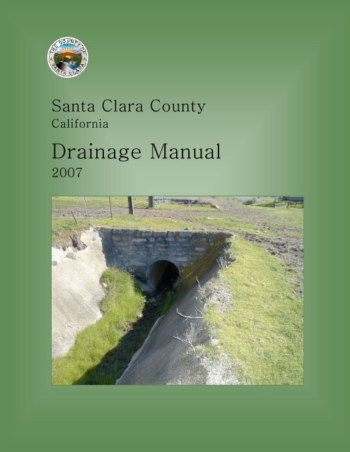
<strong>Santa</strong> <strong>Clara</strong> <strong>County</strong><br />
California<br />
<strong>Drainage</strong> <strong>Manual</strong><br />
2007
<strong>Santa</strong> <strong>Clara</strong> <strong>County</strong><br />
California<br />
<strong>Drainage</strong> <strong>Manual</strong><br />
Adopted August 14, 2007<br />
Board <strong>of</strong> Supervisors<br />
Donald F. Gage District 1<br />
Blanca Alvarado District 2<br />
Pete McHugh District 3<br />
Ken Yeager District 4<br />
Liz Kniss District 5<br />
<strong>County</strong> Executive<br />
Peter Kutras, Jr.<br />
Department <strong>of</strong> Planning and Development Services<br />
Valentin Alexeeff, Director<br />
Thomas Whisler, PE<br />
Manager, Development Services Office<br />
Christopher Freitas, PE<br />
Senior Civil Engineer<br />
Gerald Quilici, PE<br />
Senior Civil Engineer
August 14, 2007<br />
<strong>Drainage</strong> <strong>Manual</strong> 2007<br />
<strong>County</strong> <strong>of</strong> <strong>Santa</strong> <strong>Clara</strong>, California<br />
This edition <strong>of</strong> the <strong>Santa</strong> <strong>Clara</strong> <strong>County</strong> <strong>Drainage</strong> <strong>Manual</strong> has been prepared to provide<br />
engineers with the requirements for the design <strong>of</strong> storm water facilities in the <strong>County</strong>.<br />
The manual sets forth <strong>County</strong> standards for storm drainage design in accordance with<br />
the <strong>County</strong>’s subdivision and land development regulations. It is being made available<br />
to public and private engineers to provide consistent design procedures throughout the<br />
<strong>County</strong>. For more information, please contact the Land Development Engineering<br />
Department.<br />
Very truly yours,<br />
Valentin Alexeeff<br />
Director, Department <strong>of</strong> Planning<br />
and Development Services
<strong>Drainage</strong> <strong>Manual</strong> 2007<br />
<strong>County</strong> <strong>of</strong> <strong>Santa</strong> <strong>Clara</strong>, California<br />
This manual was prepared for <strong>Santa</strong> <strong>Clara</strong> <strong>County</strong> by:<br />
Schaaf & Wheeler<br />
Consulting Civil Engineers<br />
100 N. Winchester Blvd., Suite 200<br />
<strong>Santa</strong> <strong>Clara</strong>, CA 95050<br />
Phone: 408‐246‐4848<br />
www.swsv.com
Table <strong>of</strong> Contents<br />
<strong>Drainage</strong> <strong>Manual</strong> 2007<br />
<strong>County</strong> <strong>of</strong> <strong>Santa</strong> <strong>Clara</strong>, California<br />
1. INTRODUCTION .............................................................................................................. 1<br />
1.1 Purpose.........................................................................................................................1<br />
1.2 <strong>Santa</strong> <strong>Clara</strong> <strong>County</strong> .................................................................................................... 1<br />
1.3 Topography ................................................................................................................. 2<br />
1.4 Climate .........................................................................................................................2<br />
1.5 Land Uses..................................................................................................................... 2<br />
1.6 Growth ......................................................................................................................... 3<br />
1.7 <strong>Drainage</strong> Design......................................................................................................... 3<br />
2. GENERAL DRAINAGE POLICIES ................................................................................ 5<br />
2.1 Flood Protection and <strong>Drainage</strong> Terminology ....................................................... 5<br />
2.2 General Procedure...................................................................................................... 7<br />
2.3 Flood Protection Levels............................................................................................. 7<br />
2.4 Hydrologic Calculations ........................................................................................... 9<br />
2.4.1 Small <strong>Drainage</strong> Areas ........................................................................................................ 9<br />
2.4.2 Large <strong>Drainage</strong> Areas ........................................................................................................ 9<br />
2.4.3 Major Projects..................................................................................................................10<br />
2.5 Projects Falling Within <strong>Santa</strong> <strong>Clara</strong> Valley Water District Jurisdiction........ 10<br />
2.6 Projects Requiring an NPDES Permit .................................................................. 10<br />
2.7 CEQA Regulations................................................................................................... 11<br />
2.8 Other Permits............................................................................................................ 12<br />
2.9 Projects Requiring Detention Storage ................................................................. 12<br />
2.10 Project Elevation Datum ......................................................................................... 15<br />
2.11 Data Access................................................................................................................ 15<br />
3. Rational Method <strong>of</strong> Peak Flow Estimation.................................................................. 17<br />
3.1 Use <strong>of</strong> Rational Method .......................................................................................... 17<br />
i 8/14/2007
<strong>Drainage</strong> <strong>Manual</strong> 2007<br />
<strong>County</strong> <strong>of</strong> <strong>Santa</strong> <strong>Clara</strong>, California<br />
3.2 Underlying Assumptions and Limitations on Use ............................................ 17<br />
3.3 Estimating Run<strong>of</strong>f Coefficients............................................................................. 18<br />
3.4 Time <strong>of</strong> Concentration ............................................................................................ 20<br />
3.4.1 3.4.1 Natural Watersheds................................................................................................. 20<br />
3.4.2 Urbanized <strong>Drainage</strong> Basins.............................................................................................. 21<br />
3.5 Rainfall Intensity ..................................................................................................... 21<br />
3.6 Rational Method Application................................................................................ 22<br />
4. Hydrograph Method ........................................................................................................ 25<br />
4.1 Applicability ............................................................................................................. 25<br />
4.2 Computer Programs................................................................................................. 25<br />
4.3 <strong>Santa</strong> <strong>Clara</strong> Valley Water District Procedures.................................................... 26<br />
4.4 Rainfall Simulation (Design Storm)..................................................................... 27<br />
4.5 Synthetic Unit Hydrographs.................................................................................. 27<br />
4.6 Watershed Parameters............................................................................................. 28<br />
4.6.1 Basin Area ....................................................................................................................... 28<br />
4.6.2 Precipitation..................................................................................................................... 28<br />
4.6.3 Initial Abstraction ............................................................................................................ 28<br />
4.6.4 SCS Curve Number ......................................................................................................... 28<br />
4.6.5 Percent Imperviousness ................................................................................................... 30<br />
4.6.6 Basin Lag ......................................................................................................................... 30<br />
4.7 Watershed Analysis ................................................................................................. 31<br />
4.8 Base Flow ................................................................................................................... 31<br />
4.9 Channel Routing ...................................................................................................... 32<br />
4.9.1 Muskingum Routing ........................................................................................................ 32<br />
4.9.2 Modified Puls Routing..................................................................................................... 32<br />
4.9.3 Kinematic Wave Routing................................................................................................. 33<br />
4.9.4 Muskingum-Cunge Routing............................................................................................. 33<br />
4.10 Storage Routing........................................................................................................ 34<br />
8/14/2007 ii
<strong>Drainage</strong> <strong>Manual</strong> 2007<br />
<strong>County</strong> <strong>of</strong> <strong>Santa</strong> <strong>Clara</strong>, California<br />
5. Hydraulic Analysis and Design..................................................................................... 35<br />
5.1 Closed Conduits ....................................................................................................... 35<br />
5.1.1 Flow Regimes .................................................................................................................. 35<br />
5.1.2 Hydraulic Grade Line ...................................................................................................... 36<br />
5.1.3 Conduit Losses................................................................................................................. 37<br />
5.1.4 Pipe Standards..................................................................................................................42<br />
5.1.5 Culverts............................................................................................................................ 45<br />
5.1.6 Appurtenant Structures .................................................................................................... 47<br />
5.2 Open Channels ......................................................................................................... 48<br />
5.2.1 Flow Regimes .................................................................................................................. 48<br />
5.2.2 Analytical Methods.......................................................................................................... 49<br />
5.2.3 Channel Roughness.......................................................................................................... 49<br />
5.2.4 Bridge Hydraulics ............................................................................................................ 50<br />
5.2.5 Transition Losses ............................................................................................................. 52<br />
5.2.6 Channel Freeboard........................................................................................................... 52<br />
5.2.7 Hydraulic Jumps .............................................................................................................. 54<br />
5.2.8 Channel Curvature ........................................................................................................... 54<br />
5.2.9 Air Entrainment ............................................................................................................... 55<br />
5.3 Coincident Analyses................................................................................................ 56<br />
5.4 Computer Programs................................................................................................. 56<br />
6. Storage Facilities ............................................................................................................... 59<br />
6.1 Detention Facilities.................................................................................................. 59<br />
6.1.1 Types <strong>of</strong> Detention Basins............................................................................................... 59<br />
6.1.2 Outlet Structures .............................................................................................................. 61<br />
6.1.3 Overflow Spillways ......................................................................................................... 61<br />
6.1.4 Freeboard ......................................................................................................................... 62<br />
6.2 Retention Facilities .................................................................................................. 62<br />
6.3 Detention Basin Applicability and Design......................................................... 63<br />
6.3.1 Very Small Watersheds.................................................................................................... 63<br />
iii 8/14/2007
<strong>Drainage</strong> <strong>Manual</strong> 2007<br />
<strong>County</strong> <strong>of</strong> <strong>Santa</strong> <strong>Clara</strong>, California<br />
6.3.2 Other Watersheds............................................................................................................. 64<br />
6.3.3 Design Guidelines............................................................................................................ 64<br />
6.4 Computer Programs................................................................................................. 66<br />
A. Appendix A ......................................................................................................................A‐1<br />
B. Appendix B....................................................................................................................... B‐1<br />
C. Appendix C ...................................................................................................................... C‐1<br />
D. Appendix D......................................................................................................................D‐1<br />
E. Appendix E........................................................................................................................E‐1<br />
F. Appendix F........................................................................................................................F‐1<br />
G. Appendix G......................................................................................................................G‐1<br />
H. Appendix H......................................................................................................................H‐1<br />
I. Appendix I..........................................................................................................................I‐1<br />
J. Appendix J..........................................................................................................................J‐1<br />
K. Appendix K ......................................................................................................................K‐1<br />
L. Appendix L........................................................................................................................L‐1<br />
Table <strong>of</strong> Tables<br />
Table 2‐1: Freeboard Criteria for Existing Storm Drain Systems........................................... 8<br />
Table 2‐2: Summary <strong>of</strong> Hydrologic Method Criteria ............................................................ 14<br />
Table 3‐1: Run<strong>of</strong>f Coefficients for Rational Formula............................................................. 19<br />
Table 4‐1: Antecedent Moisture Conditions for Simulation................................................. 29<br />
Table 4‐2: Basin Lag Urbanization Parameters....................................................................... 31<br />
Table 5‐1: Loss Coefficients for Change in Flow Direction................................................... 40<br />
Table 5‐2: Bend Loss Coefficients in Open Channels ............................................................ 41<br />
Table 5‐3: Bridge Pier Coefficients ........................................................................................... 51<br />
8/14/2007 iv
<strong>Drainage</strong> <strong>Manual</strong> 2007<br />
<strong>County</strong> <strong>of</strong> <strong>Santa</strong> <strong>Clara</strong>, California<br />
Table 5‐4: Orifice Coefficients................................................................................................... 51<br />
Table 5‐5: Expansion and Contraction Coefficients............................................................... 52<br />
Table 5‐6: Channel Freeboard Requirements ......................................................................... 54<br />
Table B‐1: Parameters AT,D and BT,D for TDS Equation ........................................................B‐11<br />
Table B‐2: Parameters AT,D and BT,D for TDS Equation ........................................................B‐12<br />
Table D‐1: Fractions <strong>of</strong> Total Rainfall for 24‐Hour, 5‐Minute Pattern .............................. D‐5<br />
Table E‐1: Curve Numbers for AMC II ..................................................................................E‐2<br />
Table E‐2: Conversion <strong>of</strong> AMC II Curve Numbers to Other AMC Values .......................E‐3<br />
Table F‐1: Manningʹs Roughness Coefficients for Closed Conduits and Open Channels F‐<br />
2<br />
Table F‐2: Geometric Elements <strong>of</strong> Channel Sections ............................................................F‐3<br />
Table F‐3: Storm Sewer Energy Loss Coefficients.................................................................F‐4<br />
Table F‐4: Values <strong>of</strong> Ke for Determining Loss <strong>of</strong> Head Due to Sudden Enlargement in<br />
Pipes, from the Equation: H2 = K2(V1 2 /2g)......................................................................F‐5<br />
Table F‐5: Values <strong>of</strong> K2 for Determining Loss <strong>of</strong> Head Due to Gradual Enlargement in<br />
Pipes, from the Equation: H2 = K2(V1 2 /2g)......................................................................F‐5<br />
Table F‐6: Values <strong>of</strong> K3 for Determining Loss <strong>of</strong> Head Due to Sudden Contraction from<br />
the Equation: H3 = K3(V2 2 /2g)...........................................................................................F‐6<br />
Table F‐7: Entrance Head Loss Coefficients...........................................................................F‐7<br />
Table F‐8: Slopes Required to Maintain Minimum Velocities for Full and Half‐Full Flow<br />
.............................................................................................................................................F‐9<br />
Table I‐1: NHHW and Adopted 100‐Year Tide Data ...........................................................I‐4<br />
Table I‐2: Location and Datum Conversion Factors for NOAA Tidal Benchmarks in<br />
<strong>Santa</strong> <strong>Clara</strong> <strong>County</strong>............................................................................................................I‐5<br />
Table <strong>of</strong> Figures<br />
Figure 3‐1: Computation <strong>of</strong> S, Effective Stream Slope........................................................... 20<br />
Figure 5‐1: Changes in Direction <strong>of</strong> Flow at a Junction........................................................ 40<br />
v 8/14/2007
<strong>Drainage</strong> <strong>Manual</strong> 2007<br />
<strong>County</strong> <strong>of</strong> <strong>Santa</strong> <strong>Clara</strong>, California<br />
Figure 5‐2: Multiple Flows Entering a Junction ..................................................................... 41<br />
Figure 5‐3: Bridges as a Generator <strong>of</strong> Subcritical Flow (Henderson, 1966)........................ 49<br />
Figure A‐1: Overland Flow Velocity...................................................................................... A‐3<br />
Figure A‐2: Mean Annual Precipitation, <strong>Santa</strong> <strong>Clara</strong> <strong>County</strong>............................................ A‐4<br />
Figure B‐1: IDF for M.A.P. <strong>of</strong> 12 Inches..................................................................................B‐2<br />
Figure B‐2: IDF for M.A. P. <strong>of</strong> 14 Inches.................................................................................B‐3<br />
Figure B‐3: IDF for M.A.P. <strong>of</strong> 16 Inches..................................................................................B‐4<br />
Figure B‐4: IDF for M.A. P. <strong>of</strong> 18 Inches.................................................................................B‐5<br />
Figure B‐5: IDF for M.A.P. <strong>of</strong> 20 Inches..................................................................................B‐6<br />
Figure B‐6: IDF for M.A.P. <strong>of</strong> 25 Inches..................................................................................B‐7<br />
Figure B‐7: IDF for M.A. P. <strong>of</strong> 30 Inches.................................................................................B‐8<br />
Figure B‐8: IDF for M.A.P. <strong>of</strong> 35 Inches..................................................................................B‐9<br />
Figure B‐9: IDF for M.A.P. <strong>of</strong> 40 Inches................................................................................B‐10<br />
Figure C‐1: Calculation Sheet, Storm Drain Design by Rational Method ........................ C‐3<br />
Figure C‐2: Pipe Size and Hydraulic Gradient Computations........................................... C‐4<br />
Figure D‐1: Normalized Rainfall Pattern .............................................................................. D‐3<br />
Figure F‐1: Bend Head Loss Coefficients ...............................................................................F‐8<br />
Figure G‐1: Pipe Anchor Detail 1 ........................................................................................... G‐2<br />
Figure G‐2: Pipe Anchor Detail 2 ........................................................................................... G‐3<br />
Figure H‐1: Concrete Pipe Inlet Control Nomograph.........................................................H‐2<br />
Figure H‐2: Corrugated Metal Pipe Inlet Control Nomograph .........................................H‐3<br />
Figure H‐3: Box Culvert Inlet Control Nomograph ............................................................H‐4<br />
Figure H‐4: Concrete Pipe Outlet Control Nomograph......................................................H‐5<br />
Figure H‐5: Corrugated Metal Pipe Outlet Control Nomograph......................................H‐6<br />
Figure H‐6: Box Culvert Outlet Control Nomograph .........................................................H‐7<br />
Figure H‐7: Critical Depth for Circular Pipe ........................................................................H‐8<br />
8/14/2007 vi
<strong>Drainage</strong> <strong>Manual</strong> 2007<br />
<strong>County</strong> <strong>of</strong> <strong>Santa</strong> <strong>Clara</strong>, California<br />
Figure H‐8: Critical Depth for Rectangular Channel...........................................................H‐9<br />
Figure I‐1: National Oceanic and Atmospheric Administration (NOAA) Tidal<br />
Benchmarks in <strong>Santa</strong> <strong>Clara</strong> <strong>County</strong>.................................................................................I‐2<br />
Figure I‐2: Tidal Summary ‐ Adopted 100‐Year Tidal Elevation (NGVD).........................I‐3<br />
Figure J‐1: Typical Detention Pond..........................................................................................J‐2<br />
Figure J‐2: Typical Detention Pond Section (Outlet Structures) ..........................................J‐3<br />
Figure J‐3: Riser Inflow Curves ................................................................................................J‐4<br />
Figure J‐4: Typical Detention Pond Section (Emergency Overflow Spillway) 2 Options J‐5<br />
Figure J‐5: Typical Detention Pond Section (Emergency Overflow Spillway) ..................J‐5<br />
Figure J‐6: Weir Section for Emergency Overflow Spillway ................................................J‐5<br />
vii 8/14/2007
<strong>Drainage</strong> <strong>Manual</strong> 2007<br />
<strong>County</strong> <strong>of</strong> <strong>Santa</strong> <strong>Clara</strong>, California<br />
8/14/2007 viii
1. INTRODUCTION<br />
<strong>Drainage</strong> <strong>Manual</strong> 2007<br />
<strong>County</strong> <strong>of</strong> <strong>Santa</strong> <strong>Clara</strong>, California<br />
1.1 Purpose<br />
The Office <strong>of</strong> Development Services has prepared this drainage manual to provide a<br />
framework for the various hydraulic and hydrologic analyses necessary to plan and<br />
design storm drainage and flood control facilities within <strong>Santa</strong> <strong>Clara</strong> <strong>County</strong>. By<br />
providing this tool to landowners, developers, engineers and other agencies, <strong>Santa</strong> <strong>Clara</strong><br />
<strong>County</strong> anticipates that when used in conjunction with other agency manuals and<br />
design criteria, the information contained herein will help produce consistent and<br />
equivalent results.<br />
This edition <strong>of</strong> the <strong>Drainage</strong> <strong>Manual</strong> is an update to the manual published in March<br />
1966. As predicted nearly forty years ago, tremendous urbanization within the <strong>Santa</strong><br />
<strong>Clara</strong> Valley has strained many storm drainage and flood protection systems.<br />
Continuing development and redevelopment within the county will only exacerbate<br />
potential impacts to storm drainage infrastructure. This manual is thus intended to<br />
provide methodologies to evaluate the impact <strong>of</strong> development on storm drainage<br />
infrastructure and design drainage facilities and to accommodate planned growth and<br />
redevelopment.<br />
Consistent design and evaluation criteria for storm drainage systems help the Office <strong>of</strong><br />
Development Services and other agencies review storm drain and flood protection<br />
designs and impact statements for projects throughout <strong>Santa</strong> <strong>Clara</strong> <strong>County</strong>, both within<br />
and outside <strong>of</strong> incorporated areas. This manual identifies the multiple design standards,<br />
methods <strong>of</strong> analyses, and engineering tools required for the planning and design <strong>of</strong><br />
storm drainage systems and flood control facilities within the <strong>County</strong>.<br />
1.2 <strong>Santa</strong> <strong>Clara</strong> <strong>County</strong><br />
<strong>Santa</strong> <strong>Clara</strong> <strong>County</strong> encompasses 1,315 square miles at the southern end <strong>of</strong> San Francisco<br />
Bay. The county’s population (approximately 1.7 million people in 2000, representing<br />
about one‐quarter <strong>of</strong> the Bay Area’s total population) makes it the largest <strong>of</strong> the nine Bay<br />
Area counties and the fifth largest in California.<br />
Neighboring counties include San Mateo to the northwest, Alameda and San Joaquin to<br />
the north, Stanislaus to the east, Merced to the southeast, San Benito to the south, and<br />
<strong>Santa</strong> Cruz to the west.<br />
1 8/14/2007
<strong>Drainage</strong> <strong>Manual</strong> 2007<br />
<strong>County</strong> <strong>of</strong> <strong>Santa</strong> <strong>Clara</strong>, California<br />
1.3 Topography<br />
<strong>Santa</strong> <strong>Clara</strong> <strong>County</strong>’s land forms are characterized by sub‐parallel coastal mountain<br />
ranges with intervening valleys. Major topographical features include the <strong>Santa</strong> <strong>Clara</strong><br />
Valley, which is framed by the Diablo Range to the east, the <strong>Santa</strong> Cruz Mountains to<br />
the west; and the Baylands in the northwest adjacent to San Francisco Bay. Elevations<br />
range from sea level at the bay to 4,372 feet at Copernicus Peak in the Diablo Mountain<br />
Range and to 3,806 feet at Loma Prieta in the <strong>Santa</strong> Cruz Mountains.<br />
The valley floor was formed over millions <strong>of</strong> years from rainfall, run<strong>of</strong>f, and eroding<br />
sediment from the defining mountain ranges. The width <strong>of</strong> the valley floor varies from<br />
approximately 14 miles in the north to less than 1 mile centrally, and about 5 miles at the<br />
southern end.<br />
Rolling hills surround the relatively flat and fertile <strong>Santa</strong> <strong>Clara</strong> Valley. The Diablo<br />
Range, consisting mainly <strong>of</strong> grassland, chaparral and oak savannah, dominates the<br />
entire eastern half <strong>of</strong> the county. Along the western spine, the <strong>Santa</strong> Cruz Mountains<br />
contain rolling grasslands and oak‐studded foothills, mixed hardwoods and dense<br />
evergreen forests. The higher elevations <strong>of</strong> the <strong>Santa</strong> Cruz Mountains are characterized<br />
by redwood forests, steep slopes and active earthquake faults. Areas <strong>of</strong> geologic<br />
instability are prevalent in both mountain ranges.<br />
In the northwestern corner <strong>of</strong> the county on the San Francisco Peninsula, Baylands areas<br />
adjacent to the southern San Francisco Bay waters consist mostly <strong>of</strong> vast salt evaporation<br />
ponds, significant portions <strong>of</strong> which are undergoing restoration to salt marsh and<br />
wetlands.<br />
1.4 Climate<br />
The county’s regional climate is Mediterranean, generally remaining temperate<br />
throughout the year due to the areaʹs geography and proximity to the Pacific Ocean.<br />
Temperatures in the <strong>Santa</strong> <strong>Clara</strong> Valley range from 35 to 60 degrees Fahrenheit in the<br />
winter and 50 to 100 degrees Fahrenheit during the summer. Mean annual precipitation<br />
ranges from 10 inches in the inland valley areas to 56 inches at the top <strong>of</strong> the <strong>Santa</strong> Cruz<br />
Mountains.<br />
1.5 Land Uses<br />
<strong>Santa</strong> <strong>Clara</strong> Valley from San Jose north to Palo Alto (North Valley) is extensively<br />
urbanized, housing about 90 percent <strong>of</strong> the <strong>County</strong>ʹs residents. <strong>Santa</strong> <strong>Clara</strong> <strong>County</strong><br />
8/14/2007 2
<strong>Drainage</strong> <strong>Manual</strong> 2007<br />
<strong>County</strong> <strong>of</strong> <strong>Santa</strong> <strong>Clara</strong>, California<br />
south <strong>of</strong> San Jose remains predominantly rural, with the exception <strong>of</strong> the Cities <strong>of</strong> Gilroy<br />
and Morgan Hill, and the small unincorporated community <strong>of</strong> San Martin. Low density<br />
residential developments are also scattered throughout the southern valley and foothill<br />
areas.<br />
Urban growth within <strong>Santa</strong> <strong>Clara</strong> <strong>County</strong> is primarily concentrated on the valley floor<br />
with some development located in the foothills. Over 30 percent <strong>of</strong> the <strong>Santa</strong> <strong>Clara</strong><br />
Valley is residential with an additional 5 percent occupied by commercial industries,<br />
many <strong>of</strong> which are electronics and computer companies.<br />
1.6 Growth<br />
Urbanization in the second half <strong>of</strong> the twentieth century changed <strong>Santa</strong> <strong>Clara</strong> <strong>County</strong><br />
from an area <strong>of</strong> relatively isolated agricultural communities to one <strong>of</strong> continuous urban<br />
development with both suburbs and emerging urban cores. This trend is expected to<br />
continue in the first part <strong>of</strong> the twenty‐first century; although to preserve remaining<br />
open spaces, many land use agencies are proposing more intense development within<br />
established urban areas to meet an increasing population.<br />
Between 1980 and 1990, the county grew by about 200,000 people (16 percent); and by<br />
the year 2000, another 185,000 people made <strong>Santa</strong> <strong>Clara</strong> <strong>County</strong> their home (12 percent<br />
growth). Planners generally predict that the <strong>County</strong>ʹs population will continue to grow,<br />
but at a slower rate. According to the Association <strong>of</strong> Bay Area Governments, by 2010,<br />
<strong>Santa</strong> <strong>Clara</strong> <strong>County</strong>ʹs population is projected to increase by nearly 200,000 people to<br />
almost 1.9 million, and to exceed 2 million by 2020. North <strong>County</strong> areas are expected to<br />
grow the most in terms <strong>of</strong> absolute population, but South <strong>County</strong> areas are likely to<br />
grow at faster rates.<br />
1.7 <strong>Drainage</strong> Design<br />
The owner <strong>of</strong> a proposed development or redevelopment is ultimately responsible for<br />
the design <strong>of</strong> the proposed drainage works to dispose <strong>of</strong> stormwater run<strong>of</strong>f from or<br />
through an area without endangering lives or property, to the extent that it can be<br />
economically justified without unmitigated environmental impact.<br />
Designers are solely responsible for the evaluation <strong>of</strong> public safety, for providing<br />
appropriate levels <strong>of</strong> economic protection, for ensuring maintainability <strong>of</strong> drainage<br />
facilities, for assessing the environmental impacts, and for implementing the analytical<br />
procedures most appropriate for the project at hand.<br />
3 8/14/2007
<strong>Drainage</strong> <strong>Manual</strong> 2007<br />
<strong>County</strong> <strong>of</strong> <strong>Santa</strong> <strong>Clara</strong>, California<br />
This manual is not intended to supplant the judgment <strong>of</strong> qualified registered engineers<br />
with regard to storm drain analyses, evaluation, or design. Rather, the manual is to be<br />
used primarily for the standardization <strong>of</strong> design and review practices by the Office <strong>of</strong><br />
Development Services and other cities and agencies within the county who choose to<br />
use this manual, or portions there<strong>of</strong>, as an evaluation tool. The computation <strong>of</strong> design<br />
flows and the review <strong>of</strong> planned drainage facilities by the Development Services staff,<br />
however, will be in conformance with the procedures outlined herein.<br />
Since the <strong>County</strong> may assume maintenance responsibilities for completed projects, the<br />
Office <strong>of</strong> Development Services must be assured that proposed storm drain designs or<br />
flood protection projects will not require excessive maintenance, and that there are no<br />
known jurisdictional obstacles to project maintenance.<br />
8/14/2007 4
2. GENERAL DRAINAGE POLICIES<br />
<strong>Drainage</strong> <strong>Manual</strong> 2007<br />
<strong>County</strong> <strong>of</strong> <strong>Santa</strong> <strong>Clara</strong>, California<br />
Policies and procedures introduced in this chapter shall be used by the Office <strong>of</strong><br />
Development Services for the design and review <strong>of</strong> drainage systems that fall within its<br />
direct jurisdiction. In the absence <strong>of</strong> other specific design or planning guidance from<br />
another governing body, these policies are intended to apply throughout <strong>Santa</strong> <strong>Clara</strong><br />
<strong>County</strong>.<br />
This chapter defines flood protection and drainage terminology; establishes general<br />
procedures for hydrologic analyses and design; describes required levels <strong>of</strong> protection;<br />
summarizes recurrence intervals for design discharges and water surface elevations; lists<br />
recommended calculation procedures for various categories <strong>of</strong> projects based on<br />
drainage area size; and describes a general framework <strong>of</strong> regulatory considerations that<br />
may be applicable to flood protection and drainage projects.<br />
2.1 Flood Protection and <strong>Drainage</strong> Terminology<br />
Terms used with regularity throughout this manual are defined below.<br />
Annual Series – A general term for a set <strong>of</strong> any kind <strong>of</strong> data in which each item is the<br />
maximum or minimum in a year. This manual deals most <strong>of</strong>ten with annual maximum<br />
run<strong>of</strong>f and precipitation (rainfall).<br />
Design Discharge or Design Flow – The design discharge or flow is defined as the<br />
maximum flow that a structure or system <strong>of</strong> structures is expected to pass. Usually, the<br />
drainage or flood protection system is expected to safely pass the design discharge<br />
without causing damage to property or people. Design discharge is typically expressed<br />
as a peak rate <strong>of</strong> flow, with English units <strong>of</strong> cubic feet per second (cfs), and metric units<br />
<strong>of</strong> cubic meters per second (cms).<br />
Design Storm – The design storm is defined as the temporal (time variant) distribution<br />
<strong>of</strong> a specified design rainfall depth (inches) that is a function <strong>of</strong> the storm duration<br />
(hours) and frequency (years). Table D‐1 and Figure D‐1 in Appendix D provide tabular<br />
and graphical representations <strong>of</strong> the adopted 24‐hour incremental distribution (i.e.<br />
rainfall pattern) for <strong>Santa</strong> <strong>Clara</strong> <strong>County</strong>. This pattern is based on the three‐day<br />
December 1955 rainfall event, still considered to be the storm <strong>of</strong> record for Northern<br />
California.<br />
5 8/14/2007
<strong>Drainage</strong> <strong>Manual</strong> 2007<br />
<strong>County</strong> <strong>of</strong> <strong>Santa</strong> <strong>Clara</strong>, California<br />
Flood Frequency – The frequency <strong>of</strong> flood and precipitation events are described in<br />
practice and in this manual using complementary terminology. “Exceedance frequency”<br />
refers to the probability <strong>of</strong> any individual precipitation or run<strong>of</strong>f event in any water year<br />
exceeding a certain threshold. Ten‐percent peak discharge is that flow rate with a ten<br />
percent chance <strong>of</strong> being equaled or exceeded during any water year. A “one percent, 6‐<br />
hour precipitation depth” is that 6‐hour depth <strong>of</strong> rainfall that has a one percent<br />
probability (chance) <strong>of</strong> being equaled or exceeded during any water year.<br />
An alternate terminology used in practice is the “recurrence interval,” which is also<br />
referred to as a “return period.” This terminology uses a number <strong>of</strong> years to specify a<br />
flood event. For example, a “ten‐year peak discharge” would be that discharge expected<br />
to be equaled or exceeded once every ten years on the average. The “100‐year, 6‐hour<br />
precipitation depth” is the 6‐hour depth <strong>of</strong> rainfall expected to be equaled or exceeded at<br />
a location once every 100 years on the average. Annual hydrologic events are considered<br />
to be independent <strong>of</strong> one another; so there is a finite probability <strong>of</strong> exceeding the 100‐<br />
year run<strong>of</strong>f in back‐to‐back water years. Experiencing a rainfall or run<strong>of</strong>f event <strong>of</strong> a<br />
certain magnitude does not lessen the chance (probability) <strong>of</strong> experiencing another event<br />
<strong>of</strong> equal or greater magnitude in subsequent years.<br />
These two frequency terminologies are related as the reciprocal <strong>of</strong> one another. The ten‐<br />
percent event (0.10 probability) is equivalent to the ten‐year event because the reciprocal<br />
<strong>of</strong> 0.10 is 10. Similarly the one‐percent event (0.01 probability) is the 100‐year event.<br />
Freeboard – The vertical distance between an elevation <strong>of</strong> interest (e.g. water surface,<br />
hydraulic grade line, or energy grade line) and the elevation <strong>of</strong> containment, such as the<br />
top <strong>of</strong> stream bank, street grade, or floodwall. Freeboard is intended to provide for a<br />
factor <strong>of</strong> safety in the design <strong>of</strong> stormwater storage and conveyance facilities.<br />
Frequency Interval – The frequency interval (or recurrence interval) <strong>of</strong> a peak flow is the<br />
number <strong>of</strong> years, on average, in which the specified flow is expected to be equaled or<br />
exceeded one time. Exceedance probability and frequency interval are mathematically<br />
inverse <strong>of</strong> each other; thus, an exceedance probability <strong>of</strong> 0.01 is equivalent to a frequency<br />
interval <strong>of</strong> 100 years. For example, a peak flow with a 100‐year frequency interval will,<br />
on average, be equaled or exceeded once every 100 years and has an exceedance<br />
probability <strong>of</strong> 0.01 (a 1‐percent chance <strong>of</strong> being exceeded in a given year). Frequency<br />
intervals refer to the average number <strong>of</strong> occurrences over a long period <strong>of</strong> time; for<br />
example, a 100‐year flood is statistically expected to occur about 10 times in a 1,000‐year<br />
period, rather than exactly once every 100 years. Additionally, it should be noted that<br />
8/14/2007 6
<strong>Drainage</strong> <strong>Manual</strong> 2007<br />
<strong>County</strong> <strong>of</strong> <strong>Santa</strong> <strong>Clara</strong>, California<br />
the occurrence <strong>of</strong> a flood <strong>of</strong> a given frequency interval in a given year does not affect the<br />
probability <strong>of</strong> such a flood occurring again the next year.<br />
Watershed (or <strong>Drainage</strong> Area) – The total area that drains overland to a particular “point<br />
<strong>of</strong> interest.” In this manual there are three categories <strong>of</strong> “drainage area.” A Large<br />
<strong>Drainage</strong> Area drains an area greater than 200 acres. A Small <strong>Drainage</strong> Area drains an<br />
area less than or equal to 200 acres. A Very Small <strong>Drainage</strong> Area, a subset <strong>of</strong> Small,<br />
drains an area less than or equal to 50 acres.<br />
2.2 General Procedure<br />
Standards for design are expressed as the return period <strong>of</strong> the design flow. That is, the<br />
planning, analysis, and design <strong>of</strong> drainage and flood control facilities begin by<br />
establishing a required level <strong>of</strong> protection. From a hydrologic standpoint, this involves<br />
ascertaining the recurrence interval to be used. A level <strong>of</strong> protection is also associated<br />
with providing freeboard above the design water surface elevation. The design water<br />
surface elevation is also referred to as the design hydraulic grade line (HGL).<br />
As described in this chapter, specific hydrologic methods used to calculate design<br />
discharges, size facilities, and to establish HGLs depend on the area tributary to the<br />
subject flood protection or drainage facility, as does the recurrence interval used for<br />
analysis or design.<br />
Projects in <strong>Santa</strong> <strong>Clara</strong> <strong>County</strong> shall be designed such that the stormwater run<strong>of</strong>f<br />
generated from the 10‐year design storm is conveyed in the storm drainage system<br />
(underground pipes and/or stable open channels) and the stormwater run<strong>of</strong>f generated<br />
from the 100‐year design storm is safely conveyed away from the project site without<br />
creating and/or contributing to downstream or upstream flooding conditions.<br />
2.3 Flood Protection Levels<br />
The following levels <strong>of</strong> flood protection are considered to be the minimum acceptable<br />
for new projects within <strong>Santa</strong> <strong>Clara</strong> <strong>County</strong>.<br />
Ten‐year run<strong>of</strong>f shall be contained by a storm drain system consisting <strong>of</strong> underground<br />
pipe and/or stable open channels. New storm sewers and channels shall be designed to<br />
safely convey the 10‐year storm without surcharge. Existing storm drain facilities may<br />
be used to convey flow, as long as one foot <strong>of</strong> freeboard meeting the criteria set forth in<br />
Table 2‐1 is satisfied for the new ten‐year design flow.<br />
7 8/14/2007
<strong>Drainage</strong> <strong>Manual</strong> 2007<br />
<strong>County</strong> <strong>of</strong> <strong>Santa</strong> <strong>Clara</strong>, California<br />
Table 2‐1: Freeboard Criteria for Existing Storm Drain Systems<br />
System Type Freeboard Criterion (1 foot)<br />
Storm Drains in Paved Areas<br />
Storm Drains in Unpaved<br />
Areas<br />
Open Channels<br />
8/14/2007 8<br />
From HGL to Nearest Flow Line (Gutter<br />
for Streets)<br />
From HGL to Nearest Manhole or Field<br />
Inlet Rim Elevation<br />
From HGL to Lowest Adjacent Bank<br />
Elevation<br />
As shown in Table 2‐1 existing storm drain facilities shall not be considered adequate<br />
unless they are capable <strong>of</strong> conveying the 10‐year run<strong>of</strong>f with one foot <strong>of</strong> freeboard<br />
between the 10‐year water surface elevation and the nearest gutter elevation (storm<br />
drains in paved areas), nearest manhole or filed inlet rim elevation (storm drains in<br />
unpaved areas) or lowest adjacent bank elevation (open channels). The failure <strong>of</strong> the<br />
existing storm drainage system to provide the required freeboard may necessitate storm<br />
drainage system upgrades and/or replacement and/or on‐site detention as a condition <strong>of</strong><br />
approval for proposed development.<br />
Flows in excess <strong>of</strong> the ten percent flood up to the one percent flood shall be conveyed in<br />
the streets, provided that development is not subject to flooding. Excess stormwater<br />
volume may also be detained in open space areas and parking lots, provided that<br />
development is not subject to flooding.<br />
A safe release shall be provided for the design 100‐year flow. Within urbanized areas,<br />
the 100‐year discharge may be carried by a combination <strong>of</strong> a storm drain system and<br />
surface flow on the street, as long as the hydraulic grade line is contained within street<br />
rights‐<strong>of</strong>‐way. Under no circumstances shall the energy grade line (water surface plus<br />
velocity head) exceed the finished floor elevation <strong>of</strong> any structure, including garages.<br />
Gravity drainage is to be utilized ins<strong>of</strong>ar as practicable. Areas draining to a closed sump<br />
shall be drained utilizing pumping facilities provided with standby power and<br />
automatic transfer switches.<br />
Improvements to facilities that are part <strong>of</strong> a FEMA Flood Insurance Study must be<br />
designed to contain the FEMA 100‐year water surface elevation using FEMA criteria as<br />
discussed in Chapter 5.
<strong>Drainage</strong> <strong>Manual</strong> 2007<br />
<strong>County</strong> <strong>of</strong> <strong>Santa</strong> <strong>Clara</strong>, California<br />
At the project engineers’ or <strong>County</strong>’s discretion, more stringent design standards for<br />
flood protection levels may be applied on a case‐by‐case basis if the return periods or<br />
freeboard given above fail to provide sufficient public safety, if the economic<br />
consequences <strong>of</strong> project failure warrant increased flood protection, or if more stringent<br />
standards are judged to be in the public’s or project’s best interest.<br />
Proposals for projects with design return periods or freeboard less than those provided<br />
above may be considered only when supported by clear evidence that economic<br />
considerations warrant reduced standards. In these cases, project sponsors must select<br />
appropriate design criteria on the basis <strong>of</strong> economic analyses and demonstrate that the<br />
proposed return period and freeboard provide adequate protection. Such analyses shall<br />
be submitted for approval by the Department <strong>of</strong> Planning and Development Services. In<br />
no case will economic considerations take precedence over public safety or over<br />
providing adequate flood protection to other properties.<br />
2.4 Hydrologic Calculations<br />
2.4.1 Small <strong>Drainage</strong> Areas<br />
The Rational Method (Chapter 3) may be utilized to estimate peak discharges for site<br />
projects with tributary areas less than or equal to 200 acres, where storage effects are not<br />
significant. The Rational Method is generally considered acceptable to determine peak<br />
design discharges for small urban catchments. Despite falling under the catchment area<br />
criterion for smaller site projects, the Rational Method should not be used for tributary<br />
areas less than or equal to 200 acres if: the watershed has a large percentage <strong>of</strong> pervious<br />
area with widely varying soil types, or there is substantial surface storage considered to<br />
effectively reduce the peak discharge or, with the exception <strong>of</strong> Very Small <strong>Drainage</strong><br />
Areas, when detention basin computations are required.<br />
2.4.2 Large <strong>Drainage</strong> Areas<br />
The Unit Hydrograph Method described in Chapter 4 shall be used to estimate peak<br />
discharges for site projects with tributary areas greater than 200 acres, or where run<strong>of</strong>f<br />
storage is a significant consideration. The Unit Hydrograph Method shall also be<br />
utilized on catchments with a high percentage <strong>of</strong> pervious area or with widely varying<br />
soil types, and to evaluate all but the simplest detention basins (i.e., those with very<br />
small drainage areas).<br />
9 8/14/2007
<strong>Drainage</strong> <strong>Manual</strong> 2007<br />
<strong>County</strong> <strong>of</strong> <strong>Santa</strong> <strong>Clara</strong>, California<br />
2.4.3 Major Projects<br />
While the Unit Hydrograph Method described in Chapter 4 is one means <strong>of</strong> providing<br />
design discharge estimates for projects involving major flood protection or drainage<br />
facilities, methodologies to estimate design flows from streamflow records, regression<br />
analyses and other stochastic techniques are beyond the scope <strong>of</strong> this drainage manual.<br />
For projects utilizing or impacting such facilities, planners and designers are referred to<br />
the <strong>Santa</strong> <strong>Clara</strong> Valley Water District for further guidance. 1<br />
2.5 Projects Falling Within <strong>Santa</strong> <strong>Clara</strong> Valley Water District Jurisdiction<br />
Any project that requires a permit from the <strong>Santa</strong> <strong>Clara</strong> Valley Water District must<br />
comply with all processes and procedures as put forth by that District. Currently the<br />
District has permit jurisdiction along all watercourses in the <strong>County</strong> with a drainage<br />
area greater than 320 acres (1/2 square mile.) The District currently also has permit<br />
jurisdiction fifty (50) feet from the top <strong>of</strong> bank along each side <strong>of</strong> a watercourse whose<br />
drainage area is greater than 320 acres. Up‐to‐date District requirements can be found<br />
by contacting the District or on the District’s web site: www.valleywater.org.<br />
2.6 Projects Requiring an NPDES Permit<br />
As authorized by the Federal Clean Water Act, the National Pollutant Discharge<br />
Elimination System (NPDES) permit program controls water pollution by regulating<br />
point sources that discharge pollutants into waters <strong>of</strong> the United States. In California,<br />
the Regional Water Quality Control Boards are responsible for enforcing the federal<br />
regulations through issuance <strong>of</strong> waste discharge requirements. The California Regional<br />
Water Quality Control Board, San Francisco Bay Region (Regional Board) has<br />
jurisdiction over waters in and around the <strong>Santa</strong> <strong>Clara</strong> Valley.<br />
In order to comply with these requirements, <strong>Santa</strong> <strong>Clara</strong> <strong>County</strong>, the <strong>Santa</strong> <strong>Clara</strong> Valley<br />
Water District and 13 cities in the <strong>Santa</strong> <strong>Clara</strong> Valley have joined together to form the<br />
<strong>Santa</strong> <strong>Clara</strong> Valley Urban Run<strong>of</strong>f Pollution Prevention Program (Program). The<br />
participating members <strong>of</strong> the program (Dischargers) are required to implement the<br />
stormwater pollution management measures outlined in the <strong>Santa</strong> <strong>Clara</strong> Valley Urban<br />
Run<strong>of</strong>f Management Plan (Management Plan) to control the quality <strong>of</strong> the stormwater<br />
entering their storm drainage systems. The Management Plan establishes a framework<br />
for management <strong>of</strong> stormwater discharges, sets forth the Programʹs objectives, and<br />
contains performance standards required <strong>of</strong> each <strong>of</strong> the Dischargers.<br />
8/14/2007 10
<strong>Drainage</strong> <strong>Manual</strong> 2007<br />
<strong>County</strong> <strong>of</strong> <strong>Santa</strong> <strong>Clara</strong>, California<br />
Current NPDES regulations can be found on the web site www.scvurppp.org or by<br />
inquiring at the applicable planning or building permit authority for any project.<br />
2.7 CEQA Regulations<br />
The California Environmental Quality Act (CEQA) requires an environmental review <strong>of</strong><br />
projects proposed to be undertaken or requiring approval by State and Local<br />
government agencies. The goal <strong>of</strong> the CEQA review process is to identify the significant<br />
environmental impacts <strong>of</strong> projects and to either avoid the impacts or mitigate for them.<br />
CEQA requires that an environmental checklist form be completed in order to address<br />
whether the project would affect a number <strong>of</strong> environmental factors, including<br />
hydrology and water quality. Hydrologic and water quality issues that must be<br />
addressed in the current CEQA environmental checklist include:<br />
• Violation <strong>of</strong> any water quality standards or waste discharge requirements<br />
• Substantial depletion <strong>of</strong> groundwater supplies or interference with groundwater<br />
recharge<br />
• Substantial alteration <strong>of</strong> existing drainage patterns resulting in substantial on‐ or<br />
<strong>of</strong>f‐site erosion or siltation<br />
• Substantial alteration <strong>of</strong> existing drainage patterns resulting in substantial on‐ or<br />
<strong>of</strong>f‐site flooding<br />
• Creation or contribution <strong>of</strong> run<strong>of</strong>f water which would exceed the capacity <strong>of</strong><br />
existing or proposed stormwater drainage systems or provide substantial<br />
additional sources <strong>of</strong> polluted run<strong>of</strong>f<br />
• Other substantial degradation <strong>of</strong> water quality<br />
• Placement <strong>of</strong> housing within a 100‐year flood hazard area as mapped on a<br />
federal Flood Hazard Boundary or Flood Insurance Rate Map or other flood<br />
hazard delineation map<br />
• Placement <strong>of</strong> structures within a 100‐year flood hazard area which would<br />
impede or redirect flood flows<br />
• Exposure <strong>of</strong> people or structures to a significant risk <strong>of</strong> loss, injury or death<br />
involving flooding, including flooding as a result <strong>of</strong> the failure <strong>of</strong> a levee or dam<br />
Each <strong>of</strong> the items addressed in the CEQA environmental checklist are evaluated to<br />
determine whether the project results in no impact, less than significant impact, less than<br />
significant impact with mitigation incorporation, or potentially significant impact. If a<br />
determination <strong>of</strong> ʺless than significant impact with mitigation incorporationʺ is sought,<br />
the project applicant may be required to determine feasible mitigation alternative(s) and<br />
11 8/14/2007
<strong>Drainage</strong> <strong>Manual</strong> 2007<br />
<strong>County</strong> <strong>of</strong> <strong>Santa</strong> <strong>Clara</strong>, California<br />
demonstrate that the mitigation alternative(s), once incorporated into the project, result<br />
in less than significant environmental impacts. In terms <strong>of</strong> hydrology and water quality,<br />
mitigation alternatives may include, but not be limited to: water quality ponds,<br />
detention ponds, retention ponds, and low‐flow diversions for riparian habitat and/or<br />
wetland restoration.<br />
Up‐to‐date CEQA requirements may be obtained by requesting information from the<br />
responsible land use agency or building permit‐granting agency.<br />
2.8 Other Permits<br />
Permits from local, state, regional and federal agencies may be required to complete the<br />
construction, operation and maintenance <strong>of</strong> storm drainage and flood protection<br />
facilities. The <strong>County</strong> bears no responsibility for determining the permits required for<br />
any given project. Agencies, acts and permits listed in this chapter are common to<br />
typical storm water related projects, but are not intended to be all‐inclusive.<br />
Examples <strong>of</strong> such permits are: U.S. Army Corps <strong>of</strong> Engineers Section 404 <strong>of</strong> the Clean<br />
Water Act; National Marine Fisheries Section 10(a)(1)(B) <strong>of</strong> the Endangered Species Act;<br />
and State <strong>of</strong> California Department <strong>of</strong> Fish and Game Sections 1601 and 1603 Streambed<br />
Alteration Permit. Requirements for these and other necessary permits should be<br />
determined by contacting the permitting agency.<br />
2.9 Projects Requiring Detention Storage<br />
Detention storage may be required to mitigate for the loss <strong>of</strong> existing storage within a<br />
watershed; increased stormwater run<strong>of</strong>f due to increased imperviousness within a<br />
watershed; or the degradation <strong>of</strong> water quality resulting from proposed development<br />
within a watershed. Wherever possible, the <strong>County</strong> encourages regional detention<br />
facilities maintained by a public agency rather than individual site facilities on private<br />
property.<br />
Existing storage within a watershed may take the form <strong>of</strong> depression storage, swales,<br />
natural channels, and increased roughness due to vegetation within the watershed.<br />
Development within a watershed may reduce the amount <strong>of</strong> storage by clearing the area<br />
and increasing the amount <strong>of</strong> impervious surfaces.<br />
An increase in impervious surfaces (e.g. ro<strong>of</strong>s and pavement) resulting from<br />
development within a watershed may lead to an increase in the amount <strong>of</strong> surface water<br />
8/14/2007 12
<strong>Drainage</strong> <strong>Manual</strong> 2007<br />
<strong>County</strong> <strong>of</strong> <strong>Santa</strong> <strong>Clara</strong>, California<br />
run<strong>of</strong>f generated from the project site (both peak rate – and thus velocity – and volume).<br />
These increases are generally attributed to the loss <strong>of</strong> infiltrative capacity <strong>of</strong> the soil and<br />
the loss <strong>of</strong> vegetation within the watershed. They may also be the function <strong>of</strong> improved<br />
drainage and lost storage.<br />
A portion <strong>of</strong> the rainfall that is infiltrated into the ground is absorbed by the soil and the<br />
remaining infiltrated rainfall flows through the soil as subsurface flow, including<br />
interflow and groundwater. Precipitation is also intercepted by vegetation and released<br />
back to the atmosphere through transpiration. Finally, a portion <strong>of</strong> the rainfall is<br />
captured in depression storage within the watershed. Collectively, infiltration,<br />
interception and depression storage are referred to as “hydrologic losses.”<br />
Development within a watershed may also lead to degradation <strong>of</strong> the quality <strong>of</strong> the<br />
stormwater run<strong>of</strong>f from the project site. The increase in impervious surface due to<br />
development can result in more pollutants being discharged directly to the storm<br />
drainage system and its receiving waters. Pursuant to current NPDES requirements<br />
discussed in Section 2.6, new development or significant redevelopment shall be<br />
required to incorporate site design practices that reduce the impacts <strong>of</strong> development on<br />
water quality. The incorporation <strong>of</strong> landscape‐based measures, including detention<br />
storage, is one such site design measure.<br />
As previously discussed, unit hydrograph analyses are required for large site projects<br />
with catchments larger than 200 acres, and where detention storage is a significant<br />
component. Analyzing storm run<strong>of</strong>f hydrographs allows for a more detailed accounting<br />
<strong>of</strong> the hydrologic processes occurring within a watershed, including hydrologic losses,<br />
natural storage, routing, and the evaluation <strong>of</strong> detention systems. Hydrograph analyses<br />
shall be used to analyze the effects <strong>of</strong> detention storage for project sites draining more<br />
than 50 acres. For project sites with drainage areas smaller than 50 acres, a modified<br />
Rational Method approach suitable for analyzing the effects <strong>of</strong> detention storage<br />
described in Chapter 6 may be used.<br />
A summary <strong>of</strong> the hydrologic method criteria is shown in Table 2‐2.<br />
13 8/14/2007
<strong>Drainage</strong> <strong>Manual</strong> 2007<br />
<strong>County</strong> <strong>of</strong> <strong>Santa</strong> <strong>Clara</strong>, California<br />
Table 2‐2: Summary <strong>of</strong> Hydrologic Method Criteria<br />
A. If projects require review, approval, or permit issuance by the <strong>Santa</strong> <strong>Clara</strong> Valley Water<br />
District, then the current hydrologic calculation methods approved by the District shall be used.<br />
Generally, these types <strong>of</strong> projects include:<br />
• Projects that outfall directly into a SCVWD facility;<br />
• Projects being constructed within 50 feet <strong>of</strong> a SCVWD facility;<br />
• Major projects which involve major flood protection or drainage facilities, or<br />
which may affect major flood protection or drainage facilities.<br />
B. If projects do not require SCVWD approval and they meet all <strong>of</strong> the following bulleted<br />
criteria, then the hydrologic method as noted is to be used:<br />
• No detention being used;<br />
• No substantial surface storage effects;<br />
• No large areas <strong>of</strong> pervious soils.<br />
Size <strong>of</strong> <strong>Drainage</strong> Area Hydrologic Method to be Used<br />
200 Acres or Less<br />
(Small <strong>Drainage</strong> Area)<br />
More Than 200 Acres<br />
(Large <strong>Drainage</strong> Area)<br />
8/14/2007 14<br />
Rational Method May Be Used<br />
Unit Hydrograph Method Must Be Used<br />
C. If projects do not require SCVWD approval and they meet any <strong>of</strong> the following bulleted<br />
criteria, then the hydrologic method as noted is to be used:<br />
• Detention being used<br />
• Substantial surface storage effects<br />
• Large areas <strong>of</strong> pervious soils<br />
Size <strong>of</strong> <strong>Drainage</strong> Area Hydrologic Method to be Used<br />
50 Acres or Less<br />
(Very Small <strong>Drainage</strong> Area)<br />
Modified Rational Method May Be Used<br />
(APWA or ASCE Methods)*<br />
More Than 50 Acres Unit Hydrograph Method Must Be Used<br />
*Refer to Chapter 6, Section 6.3.1<br />
NOTE: If pr<strong>of</strong>essional consultants have any questions about what design method should be<br />
used, they should contact staff at the Development Services Office before proceeding with the<br />
design
<strong>Drainage</strong> <strong>Manual</strong> 2007<br />
<strong>County</strong> <strong>of</strong> <strong>Santa</strong> <strong>Clara</strong>, California<br />
2.10 Project Elevation Datum<br />
Currently there are a number <strong>of</strong> different vertical datum systems in use in <strong>Santa</strong> <strong>Clara</strong><br />
<strong>County</strong>. These include:<br />
• National Geodetic Vertical Datum <strong>of</strong> 1929 (NGVD 29)<br />
• North American Vertical Datum <strong>of</strong> 1988 (NAVD 88)<br />
• Mean Lower Low Water (MLLW)<br />
• Numerous local city datum systems<br />
The engineer must be cognizant <strong>of</strong> various datum systems and be certain that all<br />
elevations used for tides, channel cross‐sections, tailwater elevations, storm drain system<br />
inverts and rim elevations, and other relevant hydrologic data are on consistent vertical<br />
datum systems. Engineers should also be aware that conversions between datum<br />
systems are not universal, and depend upon site specific locations. The <strong>County</strong> assumes<br />
no responsibility for errors in datum.<br />
2.11 Data Access<br />
This report and all attachments can be found on the <strong>of</strong>ficial <strong>Santa</strong> <strong>Clara</strong> <strong>County</strong> Web site<br />
and may be downloaded free <strong>of</strong> charge. A selection <strong>of</strong> Internet resources for obtaining<br />
data from the U. S. Geological Survey (USGS) and the National Resources Conservation<br />
Service (NRCS) for hydrologic analysis is shown below. The URLs are current at the<br />
time <strong>of</strong> publication, but are <strong>of</strong> course, subject to change over time.<br />
Digital Elevation Model (DEM) Data:<br />
USGS, The National Map Seamless Data Distribution System:<br />
http://seamless.usgs.gov/<br />
USGS, San Francisco Bay Area 24K DEM Index Page:<br />
http://bard.wr.usgs.gov/htmldir/dem_html/index.html<br />
Land Use Data:<br />
USGS, 1:100,000‐scale Land Use‐Land Cover for California:<br />
http://edcwww.cr.usgs.gov/glis/hyper/guide/1_250_lulcfig/states100k/CA.html<br />
Soils Data:<br />
NRCS, State Soil Geographic (STATSGO) Database:<br />
ftp://ftp.ftw.nrcs.usda.gov/pub/statsgo/dos/arc/data/<br />
1. Download California STATSGO data (ca.zip).<br />
2. Unzip file. You will need all folders and files.<br />
15 8/14/2007
<strong>Drainage</strong> <strong>Manual</strong> 2007<br />
<strong>County</strong> <strong>of</strong> <strong>Santa</strong> <strong>Clara</strong>, California<br />
3. In GIS, ADD THEME. The STATSGO data is an ArcInfo coverage. It should be<br />
called CA in the “Spatial” folder.<br />
4. The “Comp.dbf” file contains hydrologic soil group (A, B, C, or D) information;<br />
add it to your GIS project. The file should be in the “Spatial” folder.<br />
5. Join “Comp.dbf” to the CA theme using “Muid” as the linking attribute<br />
(common field name).<br />
6. The “HYDGRP” field in “Comp.dbf” is the hydraulic soil group.<br />
Surface Water Features Spatial Data:<br />
USGS, National Hydrography Dataset:<br />
http://nhd.usgs.gov/<br />
Chapter Endnotes<br />
1 <strong>Santa</strong> <strong>Clara</strong> Valley Water District, Hydrology and Geology Unit. 1998; Draft Hydrology<br />
Procedures<br />
8/14/2007 16
<strong>Drainage</strong> <strong>Manual</strong> 2007<br />
<strong>County</strong> <strong>of</strong> <strong>Santa</strong> <strong>Clara</strong>, California<br />
3. RATIONAL METHOD OF PEAK FLOW ESTIMATION<br />
One primary hydrologic value <strong>of</strong> interest when evaluating and designing a storm drain<br />
collection system is the peak rate <strong>of</strong> flow that each element must carry. In a highly<br />
urbanized area characterized by relatively small watersheds with largely impervious<br />
areas, the Rational Method has a long history <strong>of</strong> usefulness for flood peak estimation<br />
and stormwater conveyance system design, where a full hydrograph is not required.<br />
3.1 Use <strong>of</strong> Rational Method<br />
The Rational Method is used to predict peak flows for small drainage areas that can be<br />
either natural or developed. The Rational Method can be used for culvert design,<br />
pavement drainage design, storm drain design, and some stormwater facility design.<br />
The Rational Method can provide satisfactory estimates for relating peak discharge to<br />
rainfall intensity by the formula:<br />
QT T<br />
Where: Q = peak discharge (cfs)<br />
= kCi A<br />
(3‐1)<br />
T = recurrence interval (years)<br />
k = 1.008 (most <strong>of</strong>ten rounded to 1)<br />
C = a dimensionless run<strong>of</strong>f coefficient<br />
i = the design rainfall intensity (inches per hour)<br />
for a duration equal to the time <strong>of</strong><br />
concentration for the basin<br />
A = drainage area (acres)<br />
3.2 Underlying Assumptions and Limitations on Use<br />
The Rational Method is based on the premise that under constant rainfall intensity, peak<br />
discharge occurs at the basin outlet when the entire area above the outlet contributes<br />
run<strong>of</strong>f. Known as the “time <strong>of</strong> concentration,” this value is defined as the time required<br />
for run<strong>of</strong>f to travel from the most hydraulically distant point (at a drainage divide such<br />
as a ridge) to the outlet. When using the Rational Formula, its underlying assumptions<br />
should be understood and verified for applicability to site conditions:<br />
1. The frequency interval <strong>of</strong> the computed peak flow is that <strong>of</strong> the design rainfall<br />
intensity.<br />
17 8/14/2007
<strong>Drainage</strong> <strong>Manual</strong> 2007<br />
<strong>County</strong> <strong>of</strong> <strong>Santa</strong> <strong>Clara</strong>, California<br />
2. Rainfall is spatially uniform over the catchment being considered.<br />
3. Rainfall intensity is uniform throughout the duration <strong>of</strong> the storm.<br />
4. Storm duration, as associated with the peak discharge, is equal to the time <strong>of</strong><br />
concentration (rainfall intensity averaging time) <strong>of</strong> the drainage area being<br />
considered.<br />
The Rational Method has been shown to provide reasonable estimates for peak<br />
discharges on small catchments where storage effects are not significant. The Rational<br />
Method is not recommended for drainage areas larger than 200 acres in <strong>Santa</strong> <strong>Clara</strong><br />
<strong>County</strong>, for any catchment where ponding or storage within the catchment might affect<br />
the peak discharge, or for catchments that utilize drainage facilities, particularly if they<br />
involve storage. It may be possible, in some cases, to adjust the run<strong>of</strong>f coefficient, C, in<br />
the Rational Method formula to account for storage within the catchment; however, this<br />
is not recommended since the Rational Method only provides an estimate <strong>of</strong> the peak<br />
discharge, not a discharge hydrograph. A modified Rational Method approach may be<br />
used to analyze the effects <strong>of</strong> detention storage for project sites with drainage areas less<br />
than 50 acres.<br />
3.3 Estimating Run<strong>of</strong>f Coefficients<br />
In the Rational Method, a lumped parameter, C, is used to convert precipitation into<br />
direct run<strong>of</strong>f. This parameter models all <strong>of</strong> the watershed variables (e.g., infiltration,<br />
depression storage, vegetation, evapotranspiration, etc.) that cause only a certain<br />
percentage <strong>of</strong> precipitation to flow <strong>of</strong>f <strong>of</strong> the catchment as run<strong>of</strong>f. Estimated values <strong>of</strong><br />
peak discharge, therefore, are heavily influenced by the selection <strong>of</strong> run<strong>of</strong>f coefficients.<br />
Run<strong>of</strong>f coefficients to be used in analysis and design are listed in Table 3‐1 for various<br />
land use conditions, ground covers, and hydrologic soil groups (HSG). Run<strong>of</strong>f<br />
coefficients are calibrated to generally match results obtained when using the US<br />
Department <strong>of</strong> Agriculture Soil Conservation Service (SCS but now Natural Resources<br />
Conservation Service) Curve Number methodology for representative 200‐acre<br />
watersheds, which is the threshold for using the unit hydrograph method. Run<strong>of</strong>f<br />
coefficients for watersheds with more than one land use or soil type shall be weighted<br />
based on area. Coefficients listed for “shrub land” may be considered for chaparral, an<br />
oak‐grass complex, and other non‐agricultural rural areas. Engineering judgment shall<br />
be used to modify run<strong>of</strong>f coefficients for unique land uses not listed.<br />
8/14/2007 18
<strong>Drainage</strong> <strong>Manual</strong> 2007<br />
<strong>County</strong> <strong>of</strong> <strong>Santa</strong> <strong>Clara</strong>, California<br />
In Table 3‐1 Soil Types B, C and D are based on the SCS classification <strong>of</strong> HSG. This<br />
designation is a standard designation used by the SCS and has been defined for <strong>Santa</strong><br />
<strong>Clara</strong> <strong>County</strong> in existing SCS publications. D‐type soils are less permeable than are C‐<br />
type soils, which are, in turn, less permeable than B‐type soils.<br />
Land Use<br />
Table 3‐1: Run<strong>of</strong>f Coefficients for Rational Formula<br />
C for Soil Type<br />
B C D<br />
Low Density Residential 0.30 0.40 0.45<br />
Medium Density Residential 0.50 0.55 0.60<br />
High Density Residential 0.70 0.70 0.75<br />
Commercial 0.80 0.80 0.80<br />
Industrial 0.70 0.75 0.75<br />
Parks 0.20 0.30 0.35<br />
Agricultural 0.15 0.35 0.40<br />
Urban Open Space 0.10 0.35 0.45<br />
Shrub Land 0.10 0.20 0.30<br />
Paved / Impervious Surface 0.85 0.85 0.85<br />
The Rational Method implies that this ratio is fixed for a given drainage basin. Studies<br />
have shown, however, that the coefficient may vary with respect to prior wetting and<br />
seasonal conditions (antecedent moisture). It has also been observed that as rainfall<br />
intensity increases, soil permeability decreases. One may sense that run<strong>of</strong>f coefficients<br />
should increase with rainfall intensity.<br />
Applying such non‐linearities over relatively small urbanized drainage basins does not<br />
necessarily improve hydrologic precision enough to <strong>of</strong>fset the more difficult<br />
computations, so using a constant run<strong>of</strong>f coefficient is standard in <strong>Santa</strong> <strong>Clara</strong> <strong>County</strong>.<br />
For watersheds with significant variation in antecedent moisture conditions, soil types,<br />
or other complexities, however; the hydrograph method described in Chapter 4 should<br />
be employed regardless <strong>of</strong> basin size.<br />
19 8/14/2007
<strong>Drainage</strong> <strong>Manual</strong> 2007<br />
<strong>County</strong> <strong>of</strong> <strong>Santa</strong> <strong>Clara</strong>, California<br />
3.4 Time <strong>of</strong> Concentration<br />
Effective use <strong>of</strong> the Rational Formula also depends upon the computation <strong>of</strong> the time <strong>of</strong><br />
concentration. As indicated previously, the time <strong>of</strong> concentration is defined as the travel<br />
time <strong>of</strong> a drop <strong>of</strong> water from the most hydraulically remote point in the contributing<br />
area to the point where the discharge is being determined. The travel time for the water<br />
to move down the catchment can include overland flow time and the travel time in<br />
street gutters, roadside swales, storm sewers, drainage channels, small streams, and<br />
other drainage ways.<br />
3.4.1 3.4.1 Natural Watersheds<br />
For natural watersheds with flow primarily in channels after an initial overland flow<br />
distance typically equal to about 300 feet, the Kirpich formula may be used:<br />
0.<br />
385<br />
2 ⎛ L ⎞<br />
t 0.<br />
0078 ⎜<br />
⎟<br />
c =<br />
+ 10<br />
(3‐2)<br />
⎝ S ⎠<br />
Where: tc = time <strong>of</strong> concentration (minutes)<br />
L = maximum length <strong>of</strong> travel from headwater to outlet (feet)<br />
S = effective slope along L (feet per foot)<br />
The concept <strong>of</strong> effective slope is illustrated by Figure 3‐1, showing how the slope <strong>of</strong> the<br />
main hydraulic length is determined by plotting a pr<strong>of</strong>ile <strong>of</strong> the channel from the outlet<br />
to the divide along the main channel and the primary upstream overland flow path. A<br />
straight slope line is drawn on the pr<strong>of</strong>ile so that the area under the line is the same as<br />
that under the pr<strong>of</strong>ile.<br />
Figure 3‐1: Computation <strong>of</strong> S, Effective Stream Slope<br />
8/14/2007 20
3.4.2 Urbanized <strong>Drainage</strong> Basins<br />
Run<strong>of</strong>f from urbanized basins travels in three phases:<br />
<strong>Drainage</strong> <strong>Manual</strong> 2007<br />
<strong>County</strong> <strong>of</strong> <strong>Santa</strong> <strong>Clara</strong>, California<br />
1. Initial overland flow represents rainfall collecting on ro<strong>of</strong> tops and making its way to<br />
an impervious surface, where run<strong>of</strong>f begins in earnest. This value is assumed to be<br />
ten minutes where a substantial area is drained, and five minutes when only street<br />
or parking lot sections are drained.<br />
2. Gutter flow represents the sheet flow <strong>of</strong> run<strong>of</strong>f over pavement, other impervious<br />
surfaces (e.g. street gutters), or pervious surfaces toward an initial collection point in<br />
the storm drain system. Calculations for this portion <strong>of</strong> the initial travel time shall be<br />
based upon nomographs included as Figure A‐1 in Appendix A.<br />
3. Pipe flow in a storm drain collection system shall be calculated by dividing the<br />
distance between design points by the average flow velocity in the subject reach <strong>of</strong><br />
pipe. (More detailed procedures regarding storm drain hydraulics are provided in<br />
Chapter 5 <strong>of</strong> this manual.) Since flow velocities may change between inlets or<br />
manholes due to changes in flow rate, pipe size, roughness, or slope, the total pipe<br />
flow time must be calculated as the sum <strong>of</strong> the time increments for each section <strong>of</strong><br />
storm drain.<br />
The total time <strong>of</strong> concentration to be used in the Rational Method calculation is the sum<br />
<strong>of</strong> the overland flow time plus any travel time in pipes, gutters, swales, or channels<br />
leading down to the point where the discharge is being determined.<br />
3.5 Rainfall Intensity<br />
Calculated times <strong>of</strong> concentration are used to establish the average rainfall intensity to<br />
be applied uniformly over the watershed to produce its peak discharge for a specified<br />
return period using the Rational Formula.<br />
The <strong>Santa</strong> <strong>Clara</strong> Valley Water Districtʹs Return Period‐Duration‐Specific (TDS) Regional<br />
Equation has been used to establish a relationship between precipitation depth and<br />
Mean Annual Precipitation for various storm frequencies (return periods).<br />
Mean Annual Precipitation isohyets for <strong>Santa</strong> <strong>Clara</strong> <strong>County</strong> have been excerpted from<br />
the <strong>Santa</strong> <strong>Clara</strong> Valley Water District 1 and presented as Figure A‐2 in Appendix A. In<br />
areas where the isohyet gradient is relatively constant, particularly for smaller basins,<br />
the Mean Annual Precipitation value used to select an IDF curve or apply Equation 3‐3<br />
may be selected at the watershed’s centroid, or weighted center <strong>of</strong> an area. In larger<br />
areas, particularly those with rapidly changing Mean Annual Precipitation contours,<br />
21 8/14/2007
<strong>Drainage</strong> <strong>Manual</strong> 2007<br />
<strong>County</strong> <strong>of</strong> <strong>Santa</strong> <strong>Clara</strong>, California<br />
such as mountain slopes, the catchment’s representative Mean Annual Precipitation<br />
value should be obtained by true areal averaging. The true areal averaging method may<br />
also be most appropriate for larger watersheds <strong>of</strong> unusual shapes such as: crescents,<br />
inverted pear, extremely elongated, or bent.<br />
Twenty‐four‐hour storm durations are used to establish rainfall intensity‐duration‐<br />
frequency (IDF) curves provided in Appendix B. The TDS Regional Equation is given<br />
by:<br />
( B MAP)<br />
xT , D = AT<br />
, D + T , D<br />
(3‐3)<br />
Where: xT,D = precipitation depth for a specific return period and storm<br />
duration (inches)<br />
T = return period (years)<br />
D = storm duration (hours)<br />
AT,D, BT,D = coefficients from Tables B‐1 and ‐2 (dimensionless)<br />
MAP = Mean Annual Precipitation (inches)<br />
The precipitation intensity, iT,D is given by:<br />
xT<br />
, D<br />
iT<br />
, D = (3‐4)<br />
D<br />
Intensity‐Duration‐Frequency (IDF) curves for Mean Annual Precipitation (MAP) values<br />
<strong>of</strong> 15‐, 20‐, 25‐, 30‐, 35‐, and 40‐inches are provided for users’ convenience in Appendix<br />
B. Intensity curves for 2‐, 5‐, 10‐, 25‐, 50‐, and 100‐year return periods are shown for<br />
each <strong>of</strong> the IDF curves. Interpolation may be used to obtain IDF relationships for MAP<br />
values between those shown in Appendix B, or Equations 3‐3 and 3‐4 can be applied<br />
directly.<br />
3.6 Rational Method Application<br />
Calculation sheets to assist manual users with Rational Method computations are<br />
provided in Appendix C. Generally, the Rational Formula is applied by breaking up the<br />
storm drain system and watershed <strong>of</strong> interest into discrete points <strong>of</strong> concentration. Land<br />
uses and soil types within the individual catchments are tabulated by area, and<br />
component run<strong>of</strong>f coefficients are obtained using Table 3‐1. A composite run<strong>of</strong>f<br />
coefficient is obtained by areal weighting. Times <strong>of</strong> concentration for each catchment are<br />
calculated using the procedures described herein, and using the appropriate IDF curve<br />
8/14/2007 22
<strong>Drainage</strong> <strong>Manual</strong> 2007<br />
<strong>County</strong> <strong>of</strong> <strong>Santa</strong> <strong>Clara</strong>, California<br />
from Appendix B, rainfall intensity is input into the Rational Formula to provide the<br />
estimated peak discharge at each point <strong>of</strong> concentration.<br />
For small areas, particularly in the upstream reaches <strong>of</strong> a system, it may be that the<br />
highest peak flow will be computed by using a shorter time <strong>of</strong> concentration from an<br />
individual catchment instead <strong>of</strong> the cumulative time <strong>of</strong> concentration resulting from<br />
travel in the upstream collection system. The peak flow computed from a smaller area,<br />
but more intense rainfall intensity due to the short time <strong>of</strong> concentration, may control<br />
the design in the most upstream portion <strong>of</strong> the drainage system, but as the design moves<br />
downstream to larger areas, usually the cumulative effective area (C x A) and longer<br />
time <strong>of</strong> concentration result in higher flows. Whichever combination <strong>of</strong> cumulative C x<br />
A and cumulative time <strong>of</strong> concentration produces the highest peak discharge at any<br />
given point shall govern the design <strong>of</strong> the drainage system immediately downstream <strong>of</strong><br />
that point.<br />
Chapter End Notes<br />
1<br />
<strong>Santa</strong> <strong>Clara</strong> Valley Water District, Mean Annual Precipitation Map, San Francisco and<br />
Monterey Bay Region [map]. 1:250,000. 1988.<br />
23 8/14/2007
<strong>Drainage</strong> <strong>Manual</strong> 2007<br />
<strong>County</strong> <strong>of</strong> <strong>Santa</strong> <strong>Clara</strong>, California<br />
8/14/2007 24
4. HYDROGRAPH METHOD<br />
<strong>Drainage</strong> <strong>Manual</strong> 2007<br />
<strong>County</strong> <strong>of</strong> <strong>Santa</strong> <strong>Clara</strong>, California<br />
4.1 Applicability<br />
The hydrograph method is generally used when analyzing larger watersheds where the<br />
Rational Method should not be applied. The hydrograph method allows the user to<br />
account for hydrologic losses, including evaporation, transpiration, infiltration, surface<br />
routing, storage within the watershed, and varying antecedent moisture conditions. In<br />
addition, the hydrograph method allows for the analysis <strong>of</strong> complex drainage facilities,<br />
including diversions and detention ponds. In practice, this method allows for the<br />
development <strong>of</strong> a flood hydrograph using a design storm, an appropriate infiltration or<br />
loss rate technique, and a synthetic unit hydrograph.<br />
The basic process <strong>of</strong> the hydrograph method includes:<br />
• Simulating rainfall from a specified storm event<br />
• Simulating rainfall losses due to interception and infiltration<br />
• Simulating the overland flow into creeks, channels, or pipes to provide a run<strong>of</strong>f<br />
hydrograph at concentrated points<br />
• Routing the hydrograph through creeks, channels, or pipes<br />
• Routing the hydrograph through detention basins or reservoirs<br />
Detailed explanation <strong>of</strong> the hydrograph method can be found in the Handbook <strong>of</strong> Applied<br />
Hydrology by V. T. Chow, 1 Hydrology for Engineers by Linsley, Kohler, and Paulhus, 2 the<br />
ASCE <strong>Manual</strong> and Report on Engineering Practice No. 28, Hydrology Handbook, 3 and<br />
other appropriate references.<br />
A hydrograph analysis is required for drainage areas greater than 200 acres, or if the<br />
drainage area is greater than 50 acres and includes a detention basin or storage reservoir.<br />
For areas less than 200 acres or those smaller areas that do not require a detention basin<br />
or storage reservoir, the hydrograph method may be applied, but should be compared to<br />
the results obtained by application <strong>of</strong> the Rational Method described in Chapter 3.<br />
4.2 Computer Programs<br />
HEC‐1 and HEC‐HMS are hydrologic modeling computer programs developed by the<br />
Hydrologic Engineering Center (HEC) <strong>of</strong> the U. S. Army Corps <strong>of</strong> Engineers. Both<br />
programs are designed to compute rainfall‐run<strong>of</strong>f hydrographs and route the<br />
hydrographs through channels, pipes, detention basins, and reservoirs. HEC‐1 is a<br />
25 8/14/2007
<strong>Drainage</strong> <strong>Manual</strong> 2007<br />
<strong>County</strong> <strong>of</strong> <strong>Santa</strong> <strong>Clara</strong>, California<br />
DOS‐based program that receives its input data via a text file. It was originally released<br />
in 1968; the current version (Version 4.0) was released in 1990. HEC‐HMS, originally<br />
released in 1998, is a Windows‐based program that provides a Graphical User Interface<br />
(GUI) intended to simplify data input. HEC‐HMS has many <strong>of</strong> the same capabilities as<br />
HEC‐1.<br />
This manual is not intended to be a user’s guide for either HEC‐1 or HEC‐HMS. It is<br />
assumed that the reader is familiar with one or both <strong>of</strong> these programs. However, if you<br />
are unfamiliar with either program, user’s manuals for both can be downloaded from<br />
HEC’s homepage, http://www.hec.usace.army.mil.<br />
HEC‐1 and HEC‐HMS follow the same basic procedure for hydrologic modeling<br />
described in this section. It is important to recognize that these computer programs are<br />
intended only to simulate naturally‐occurring events. In many instances, the simulated<br />
processes or results can vary significantly from those that occur naturally. Whenever<br />
possible, the simulated results should be calibrated with verified results, or at a<br />
minimum, analyzed to determine whether the results are reasonable for the given<br />
meteorologic, topographic, and land use conditions.<br />
Other hydrologic modeling s<strong>of</strong>tware packages are available, which include, but are not<br />
limited to the following:<br />
• TR‐20 and TR‐55 developed by the Natural Resources Conservation Service<br />
(NRCS)<br />
• Storm Water Management Model (SWMM) developed by the U. S.<br />
Environmental Protection Agency (EPA)<br />
• Hydrological Simulation Program‐Fortran (HSPF), originally developed as the<br />
Stanford Watershed Model<br />
• HYDRO from the Federal Highway Administration (FHWA)<br />
• MIKE SHE, available from the Danish Hydraulics Institute (DHI)<br />
Any hydrology method, including those listed above, may be used, provided the chosen<br />
method provides results consistent with those obtained using the <strong>County</strong>ʹs hydrology<br />
procedures.<br />
4.3 <strong>Santa</strong> <strong>Clara</strong> Valley Water District Procedures<br />
Projects falling within the District’s jurisdiction shall be coordinated with the District<br />
and shall be completed using standards and procedures established by the District.<br />
8/14/2007 26
<strong>Drainage</strong> <strong>Manual</strong> 2007<br />
<strong>County</strong> <strong>of</strong> <strong>Santa</strong> <strong>Clara</strong>, California<br />
4.4 Rainfall Simulation (Design Storm)<br />
“Design storm” is a term used to describe the total rainfall depth, which is determined<br />
from the combination <strong>of</strong> the return period and storm duration. Chapter 2 describes the<br />
design storms to be used for hydrologic and hydraulic analysis and facility design. In<br />
<strong>Santa</strong> <strong>Clara</strong> <strong>County</strong>, rainfall is the only type <strong>of</strong> precipitation considered to cause run<strong>of</strong>f;<br />
significant snowfall is rare, and snowmelt does not contribute to run<strong>of</strong>f during flood<br />
events.<br />
For most analyses and designs in the <strong>County</strong>, rainfall events <strong>of</strong> interest are those with 2‐,<br />
10‐, and 100‐year return periods. The standard storm duration for rainfall simulation is<br />
24 hours. Figure D‐1 in Appendix D provides the adopted 24‐hour incremental rainfall<br />
distribution pattern for <strong>Santa</strong> <strong>Clara</strong> <strong>County</strong>. This pattern is based upon the three‐day<br />
December 1955 rainfall event, still considered to be the storm <strong>of</strong> record for northern<br />
California.<br />
The precipitation pattern has been adjusted to preserve the local rainfall statistics in<br />
<strong>Santa</strong> <strong>Clara</strong> <strong>County</strong> based on the District’s TDS equations, which are consistent with the<br />
IDF curves provided in Appendix B. Thus, the incremental precipitation pattern<br />
provided in Figure D‐1 is balanced so that the 24‐hour storm distribution may be used<br />
even where shorter duration storms are more critical. Table D‐1 provides tabulated<br />
values <strong>of</strong> precipitation as a percentage <strong>of</strong> the total 24‐hour depth.<br />
The rainfall pattern (hyetograph) can be obtained for any watershed by multiplying the<br />
incremental rainfall distribution percentages by the 24‐hour rainfall depth (calculated<br />
using the methodology provided in Chapter 3).<br />
4.5 Synthetic Unit Hydrographs<br />
A unit hydrograph is a numerical representation <strong>of</strong> the time response <strong>of</strong> catchment<br />
run<strong>of</strong>f caused by one inch <strong>of</strong> excess rainfall applied uniformly over a unit <strong>of</strong> time.<br />
Several different techniques are available to estimate unit hydrographs for rainfall‐<br />
run<strong>of</strong>f calculations. The Soil Conservation Service (SCS, now the Natural Resources<br />
Conservation Service) synthetic unit hydrograph is used in this manual. This<br />
methodology requires only an estimate <strong>of</strong> basin lag, which is the time from the<br />
beginning <strong>of</strong> excess rainfall (i.e., direct run<strong>of</strong>f) to the point in time when fifty percent <strong>of</strong><br />
the run<strong>of</strong>f has passed the catch point.<br />
27 8/14/2007
<strong>Drainage</strong> <strong>Manual</strong> 2007<br />
<strong>County</strong> <strong>of</strong> <strong>Santa</strong> <strong>Clara</strong>, California<br />
4.6 Watershed Parameters<br />
The following watershed parameters are used in the unit hydrograph method, and are<br />
generally required input into the computer models listed in Section 4.2.<br />
4.6.1 Basin Area<br />
The basin area is defined as the area enclosed by the watershed draining to the basin<br />
outlet point where the discharge is to be determined. Area should be expressed in the<br />
units required for analysis. For HEC‐1, the basin area is in square miles.<br />
4.6.2 Precipitation<br />
Precipitation is the total depth <strong>of</strong> rainfall over the basin before any losses due to<br />
interception, infiltration, and surface storage. A value for 24‐hour precipitation depth<br />
shall be obtained at each basin centroid following the procedures outlined in Chapter 3.<br />
For HEC‐1, basin precipitation is input as inches.<br />
4.6.3 Initial Abstraction<br />
The initial abstraction represents rainfall that is absorbed by tree cover, depressions, and<br />
soil at the beginning <strong>of</strong> a storm. No run<strong>of</strong>f is calculated until the initial abstraction has<br />
been satisfied. The initial abstraction for pervious areas is set equal to 0.2S, where S =<br />
(1000/CN) ‐ 10. For impervious or rural areas the initial abstraction is set equal to 0.05<br />
inches.<br />
4.6.4 SCS Curve Number<br />
Direct run<strong>of</strong>f is estimated by subtracting soil infiltration and other losses from the rate <strong>of</strong><br />
rainfall. The Curve Number (CN) method is an empirical methodology derived by the<br />
Soil Conservation Service (SCS). The Curve Number reflects the potential loss for a<br />
given soil and cover complex. After satisfying the initial abstraction defined above, the<br />
soil becomes saturated at a certain rate so that a higher percentage <strong>of</strong> the accumulated<br />
rainfall becomes converted into run<strong>of</strong>f.<br />
Estimates <strong>of</strong> the CN are made based on the soil types and cover within a drainage basin.<br />
The number varies from 0 to 100, and represents the relative run<strong>of</strong>f potential for a given<br />
soil‐cover complex for given antecedent moisture conditions (that is, how wet it is prior<br />
to any precipitation event).<br />
Curve numbers for watershed modeling may be based on Table E‐1 in Appendix E,<br />
which correspond to Hydrologic Soil Groups established on the maps prepared by the<br />
8/14/2007 28
<strong>Drainage</strong> <strong>Manual</strong> 2007<br />
<strong>County</strong> <strong>of</strong> <strong>Santa</strong> <strong>Clara</strong>, California<br />
SCS for <strong>Santa</strong> <strong>Clara</strong> <strong>County</strong>. 4, 5 Curve numbers for Hydrologic Soil Group A, which is<br />
rarely found in the <strong>County</strong> outside <strong>of</strong> river beds, is not included in the table. Soil cover<br />
and land use may be obtained from aerial photographs, USGS quadrangle maps, general<br />
plans, geographic information systems, and field reconnaissance surveys.<br />
Antecedent moisture conditions (AMCs) represent prior soil saturation, depression<br />
storage conditions, and other hydrologic precursors prior to the initiation <strong>of</strong> design<br />
rainfall. The different categories <strong>of</strong> AMCs are characterized by the SCS as follows:<br />
AMC I dry soils<br />
AMC II average conditions<br />
AMC III heavy rainfall, light rainfall with low temperatures, or saturated soil<br />
Antecedent moisture conditions have been established for various return periods for use<br />
with the specific rainfall distribution pattern given in Appendix D. Each AMC has been<br />
calibrated to individual flood frequency analyses <strong>of</strong> annual stream discharge data for the<br />
San Francisquito Creek, Upper Penitencia Creek, and Bodfish Creek basins. Each gage is<br />
located in an area with very little urbanization, so the calibrated AMCs are consistent<br />
with the unit hydrograph application presented here. Flood frequency analyses have<br />
been made following procedures outlined in USGS Bulletin #17B. 6<br />
Table 4‐1 provides AMC values to be used for various return periods <strong>of</strong> interest.<br />
Engineers may modify the AMC as long as sufficient justification is provided.<br />
Table 4‐1: Antecedent Moisture Conditions for Simulation<br />
Design Return Period AMC<br />
2‐year (50 percent) II¼<br />
10‐year (10 percent) II½<br />
100‐year (1 percent) II½<br />
Antecedent moisture conditions given in Table 4‐1 are calibrated specifically for the<br />
rainfall distribution provided in Appendix D. AMC values must be recalibrated to use<br />
any other storm distribution.<br />
29 8/14/2007
<strong>Drainage</strong> <strong>Manual</strong> 2007<br />
<strong>County</strong> <strong>of</strong> <strong>Santa</strong> <strong>Clara</strong>, California<br />
Table E‐1 in Appendix E shows the Curve Numbers for different land use and soil types<br />
for AMC II. Using Table E‐2, these Curve Number values can be translated to the<br />
appropriate AMC, using linear interpolation as necessary.<br />
4.6.5 Percent Imperviousness<br />
This is the percentage <strong>of</strong> watershed covered by an impermeable surface such as ro<strong>of</strong>s,<br />
roads, sidewalks, driveways, and other hardscape. It is input into the hydrologic model<br />
as a percentage. In the absence <strong>of</strong> sufficient information to directly calculate the<br />
percentage <strong>of</strong> impervious area, ranges <strong>of</strong> typical percent imperviousness for various<br />
land use categories are provided in Table E‐3.<br />
4.6.6 Basin Lag<br />
The SCS lag equation (a modified version <strong>of</strong> the U. S. Army Corps <strong>of</strong> Engineers basin lag<br />
equation) is given below:<br />
⎛ L Lc<br />
⎞<br />
t = ( 0.<br />
862)<br />
24 N ⎜ ⎟<br />
lag<br />
⎝ S ⎠<br />
D<br />
−<br />
2<br />
(4‐1)<br />
Where tlag = SCS basin lag (hours)<br />
8/14/2007 30<br />
0.<br />
38<br />
N = watershed roughness value (dimensionless)<br />
L = longest flow path from catchment divide to outlet (miles)<br />
Lc = length along flow path from a point perpendicular with<br />
the basin centroid to its outlet (miles)<br />
S = effective slope along main watercourse from Chapter 3<br />
(feet/mile)<br />
D = duration <strong>of</strong> unit hydrograph (hours)<br />
If possible, the unit hydrograph duration, D, should be selected to lie between one‐fifth<br />
and one‐third <strong>of</strong> the smallest basin’s lag time.<br />
Basin length and slope values may be obtained from available mapping, and are<br />
considered to be discrete, measurable parameters. Watershed roughness is the lone<br />
subjective parameter to be chosen using engineering judgment. The parameter used in<br />
Equation 4‐1 should not be confused with Manning’s “n”. Table 4‐2 provides USACE<br />
recommended “N” values based on the level <strong>of</strong> urbanization within a watershed basin.
<strong>Drainage</strong> <strong>Manual</strong> 2007<br />
<strong>County</strong> <strong>of</strong> <strong>Santa</strong> <strong>Clara</strong>, California<br />
Table 4‐2: Basin Lag Urbanization Parameters<br />
Basin Condition N<br />
Natural channels, little or no urbanization 0.080<br />
Urban area with natural channels 0.050<br />
Concrete‐lined channels with ~2/3 basin<br />
urbanized<br />
0.035<br />
Full basin urbanization with storm drain systems 0.025<br />
For basins with a level <strong>of</strong> urbanization that falls somewhere between the values given<br />
above, engineers may interpolate using their judgment.<br />
4.7 Watershed Analysis<br />
Watersheds with relatively uniform ground cover, soil type, and degree <strong>of</strong> urbanization<br />
may be analyzed as a single basin with weighted values for Curve Number and percent<br />
impervious. Watersheds with significant variations in these parameters should be<br />
broken into smaller basins based on the geographic variation in parameters, if possible,<br />
to produce separate hydrographs, which can then be arithmetically combined to<br />
produce a design hydrograph at the concentration point.<br />
Basin separation particularly applies when there is a significant portion <strong>of</strong> soil from<br />
either Hydrologic Soil Groups A or B, and soil from either Groups C or D. Non‐<br />
linearities in the SCS Curve Number methodology can introduce errors when the Curve<br />
Number estimate is weighted by area when significant variance in soil type is present.<br />
Even if other hydrologic parameters are homogeneous throughout the watershed, the<br />
catchment should be split into at least two basins (A/B soils and C/D soils) and<br />
recombined for the final design hydrograph. If the soil types are widely dispersed<br />
within the watershed, the basin may be split into areas corresponding to the percentages<br />
<strong>of</strong> each soil type, but all with the same precipitation, basin lag, and percent<br />
imperviousness.<br />
4.8 Base Flow<br />
Base flow from groundwater infiltration and other sources is generally not considered to<br />
significantly impact estimates <strong>of</strong> peak flow, particularly for smaller watersheds. A base<br />
flow component was not used to calibrate antecedent moisture conditions. However, if<br />
experience or data show that a considerable base flow exists due to high water table,<br />
31 8/14/2007
<strong>Drainage</strong> <strong>Manual</strong> 2007<br />
<strong>County</strong> <strong>of</strong> <strong>Santa</strong> <strong>Clara</strong>, California<br />
reservoir releases, or other circumstances, it shall be considered as an addition to the<br />
design flood hydrograph. Base flow is to be used when sizing and designing<br />
stormwater detention or retention facilities as described in Chapter 6.<br />
4.9 Channel Routing<br />
Once design hydrographs at concentration points are calculated using the unit<br />
hydrograph method, those hydrographs are routed to simulate the movement <strong>of</strong> a flood<br />
wave through natural or man‐made channel reaches <strong>of</strong> varying shapes, sizes, and<br />
materials. Routing techniques and parameters shall be determined by the engineer, and<br />
justification <strong>of</strong> each technique shall be provided to the <strong>County</strong> for review. Common<br />
routing techniques and their typical uses are:<br />
4.9.1 Muskingum Routing<br />
This method is commonly used in practice to route flood hydrographs through reaches<br />
where a channel and its adjoining overbank areas provide the conveyance and storage <strong>of</strong><br />
flood waters. Routing parameters include a storage constant (K) and a parameter, “x,”<br />
which represents the relative effects <strong>of</strong> wedge and prism storage in the reach. An “x”<br />
value <strong>of</strong> zero represents a true reservoir, and could be used if there is a significant<br />
amount <strong>of</strong> spill out <strong>of</strong> a low flow channel with substantial valley storage. Most channels<br />
have “x” values between 0.0 and 0.2, the latter representing cases where the flood wave<br />
is expected to remain in the channel with no overbanking and valley storage to attenuate<br />
the hydrograph. The storage constant, K, is approximately equal to the travel time<br />
through the reach and may be determined from average flow velocity.<br />
To ensure the numerical stability <strong>of</strong> Muskingum Routing, each routing reach is broken<br />
into multiple routing segments so that the following relationship between K and x is<br />
maintained:<br />
( 1 − x) ∆ 2 x<br />
8/14/2007 32<br />
2<br />
1<br />
≤<br />
4.9.2 Modified Puls Routing<br />
While the Modified Puls procedure is commonly used for reservoir routing, it may also<br />
be used in channel routing. This routing method requires the input <strong>of</strong> physically<br />
meaningful and verifiable data to perform the hydrograph transformation by<br />
K<br />
t<br />
≤<br />
1<br />
(4‐2)
<strong>Drainage</strong> <strong>Manual</strong> 2007<br />
<strong>County</strong> <strong>of</strong> <strong>Santa</strong> <strong>Clara</strong>, California<br />
establishing storage‐discharge relationships. These relationships may be established<br />
using normal depth methods or detailed backwater computations. Variables include<br />
channel geometry and roughness. If possible, routing lengths should be established so<br />
that the time <strong>of</strong> travel through a reach is more than four or five time steps on the inflow<br />
hydrograph.<br />
4.9.3 Kinematic Wave Routing<br />
This routing method is used almost exclusively for urban prismatic channels, and<br />
computer programs employing this method generally limit its application to<br />
predetermined channel shapes. Hydrographs routed by the kinematic wave procedure<br />
are translated downstream, but there is no attenuation.<br />
4.9.4 Muskingum‐Cunge Routing<br />
The Muskingum‐Cunge routing method is a non‐linear routing technique that accounts<br />
for diffusion in the equations <strong>of</strong> motion and uses the Muskingum X‐value to assess the<br />
effects <strong>of</strong> storage in the reach. The procedure estimates the X‐value based on physical,<br />
rather than empirical, characteristics <strong>of</strong> the channel cross section, namely the reach<br />
length, slope, kinematic wave celerity, and the characteristic unit discharge at each time<br />
and stage increment. In practice it is believed to be a better routing technique than the<br />
kinematic wave procedure as it accounts for storage and not only translates the<br />
hydrograph but attenuates the hydrograph depending upon the computed X‐values as a<br />
function <strong>of</strong> time. The major disadvantage <strong>of</strong> the Muskingum‐Cunge method is that it<br />
assumes normal depth in the channel cross sections and won’t account for backwater<br />
effects that produce M‐1 or S‐1 curves<br />
Each <strong>of</strong> these flood routing methods is described in the HEC‐1 Userʹs <strong>Manual</strong>. In<br />
general, these methods are based on the continuity equation and some relationship<br />
between flow and storage or stage. In all <strong>of</strong> the methods, routing proceeds on an<br />
independent‐reach basis from upstream to downstream without the consideration <strong>of</strong><br />
backwater effects or discontinuities in the water surfaces. The Kinematic Wave method<br />
results primarily in the translation <strong>of</strong> the run<strong>of</strong>f hydrograph, with little to no<br />
attenuation, therefore it is only appropriate for short reaches <strong>of</strong> prismatic, concrete‐lined<br />
channels.<br />
33 8/14/2007
<strong>Drainage</strong> <strong>Manual</strong> 2007<br />
<strong>County</strong> <strong>of</strong> <strong>Santa</strong> <strong>Clara</strong>, California<br />
4.10 Storage Routing<br />
Storage routing is used to simulate the movement <strong>of</strong> a flood wave through a storage<br />
reservoir. By providing HEC‐1 or HEC‐HMS with information about storage (either by<br />
specifying volumes or an elevation‐surface area relationship) and outflow, it models the<br />
inflow, storage, and outflow in the storage reservoir. In HEC‐1, outflow information can<br />
be supplied in two ways, either by specifying actual discharges or by giving orifice and<br />
weir dimensions. In HEC‐HMS, outflow information can be supplied only by the<br />
former method.<br />
Chapter End Notes<br />
1Chow, Ven Te, 1964, Handbook <strong>of</strong> Applied Hydrology: A Compendium <strong>of</strong> Water Resources<br />
Technology New York: McGraw‐Hill.<br />
2Linsley, Ray K., Max Adam Kohler, and Joseph L. H. Paulhus, 1982; Hydrology for<br />
Engineers. New York: McGraw‐Hill.<br />
3American Society <strong>of</strong> Civil Engineers. Task Committee on Hydrology Handbook <strong>of</strong><br />
Management Group D. 1996. Hydrology Handbook. New York.<br />
4 Soil Conservation Service. 1968. Soils <strong>of</strong> <strong>Santa</strong> <strong>Clara</strong> <strong>County</strong>.<br />
5 Soil Conservation Service. 1974. Soil Survey <strong>of</strong> Eastern <strong>Santa</strong> <strong>Clara</strong> Area, California.<br />
6U. S. Geological Survey. Interagency Committee on Water Data. 1982. Bulletin #17B <strong>of</strong><br />
the Hydrology Subcommittee: Guidelines for Determining Flood Flow Frequency.<br />
8/14/2007 34
<strong>Drainage</strong> <strong>Manual</strong> 2007<br />
<strong>County</strong> <strong>of</strong> <strong>Santa</strong> <strong>Clara</strong>, California<br />
5. HYDRAULIC ANALYSIS AND DESIGN<br />
Storm drainage and flood protection systems must be sized so that design flows<br />
calculated using one <strong>of</strong> the methodologies outlined in Chapters 3 and 4 can be collected,<br />
conveyed, and safely discharged to receiving waters while meeting the requirements<br />
discussed in Chapter 2. This chapter presents methodologies for analyzing hydraulic<br />
gradients to determine whether a particular system can meet its design requirements.<br />
Both closed conduit and open channel systems are discussed.<br />
5.1 Closed Conduits<br />
Conveyance systems that carry storm run<strong>of</strong>f such as pipes and culverts, regardless <strong>of</strong><br />
shape, are closed conduit systems. These systems may carry storm water under<br />
pressure (surcharged), or with a free water surface pr<strong>of</strong>ile exposed to the atmosphere.<br />
With a free water surface, the flow is considered to be “open channel,” but the methods<br />
for calculating hydraulic gradients are described in this section.<br />
5.1.1 Flow Regimes<br />
Flows can be carried within closed conduits and channels either as “subcritical” flow or<br />
“supercritical” flow, <strong>of</strong>ten referred to as “tranquil” and “rapid” flow, respectively. It is<br />
not the velocity <strong>of</strong> flow, however, that distinguishes the flow regime; rather, the flow<br />
regime is defined by how fast the water is moving relative to the velocity <strong>of</strong> the wave<br />
that results from a small disturbance in the water surface. Disturbances in subcritical<br />
flow move upstream; disturbances in supercritical flow cannot move upstream because<br />
such waves must be swept downstream. The Froude number (Fr), which is analogous to<br />
the Mach number for gas flow, is defined as the ratio <strong>of</strong> conduit or channel velocity to<br />
wave velocity:<br />
v<br />
Fr = (5‐1)<br />
gy<br />
Where: v = average flow velocity (feet per second)<br />
g = gravitational acceleration (feet per second per second)<br />
y = flow depth (feet)<br />
35 8/14/2007
<strong>Drainage</strong> <strong>Manual</strong> 2007<br />
<strong>County</strong> <strong>of</strong> <strong>Santa</strong> <strong>Clara</strong>, California<br />
A Froude number greater than unity signifies supercritical flow (flow velocity greater<br />
than wave velocity), while a Froude number less than one indicates subcritical flow.<br />
When the Froude number is between 0.8 and 1.2, however, the flow can be unstable,<br />
characterized by standing waves and other disturbances that may tend to propagate<br />
upstream or downstream depending upon the state <strong>of</strong> flow.<br />
Since Froude numbers depend on conduit and channel roughness, and “n” values are<br />
expected to vary within any given reach, hydraulic gradients should be analyzed for a<br />
range <strong>of</strong> “n” as described in this chapter to protect against unexpected changes in the<br />
flow regime which could compromise the design. The high end <strong>of</strong> the “n” value range<br />
should be used to establish required freeboard, and the lower end <strong>of</strong> conduit and<br />
channel roughness are used to examine erosion potential and hydraulic stability with<br />
possibly mixed or supercritical flow conditions.<br />
5.1.2 Hydraulic Grade Line<br />
In non‐surcharged pipe flow, the hydraulic grade line (HGL) represents the water<br />
surface pr<strong>of</strong>ile. For surcharged pressure flow, the HGL represents a pr<strong>of</strong>ile <strong>of</strong> the<br />
piezometric water surface; that is, the level to which water would rise along a conduit if<br />
it were allowed to do so. For subcritical flow conditions described in Section 5.1.1, the<br />
HGL is calculated as a backwater pr<strong>of</strong>ile beginning at the most downstream point <strong>of</strong> the<br />
storm drain or outfall. For supercritical flow conditions, the HGL is calculated as a<br />
forewater pr<strong>of</strong>ile beginning at the most upstream point <strong>of</strong> the storm drain system or<br />
inlet.<br />
The water surface elevation at the storm drain outfall (subcritical flow) or inlet to the<br />
storm drain system (supercritical flow) must be known or calculated prior to an analysis<br />
<strong>of</strong> the conduit system since it acts as the starting elevation <strong>of</strong> the HGL. The HGL at the<br />
first junction in the pipe system can then be calculated by:<br />
5.1.2.1 Subcritical Flow<br />
8/14/2007 36<br />
HGLJ1 = WSELoutfall + Hf + HL (5‐2)<br />
Where: HGLJ1 = hydraulic grade line at Junction 1<br />
WSELoutfall = water surface elevation at system outfall<br />
Hf = friction loss in pipe from outfall to Junction 1<br />
HL = minor losses in pipeline from outfall to Junction 1
5.1.2.2 Supercritical Flow<br />
<strong>Drainage</strong> <strong>Manual</strong> 2007<br />
<strong>County</strong> <strong>of</strong> <strong>Santa</strong> <strong>Clara</strong>, California<br />
HGLJ1 = WSELinlet ‐ Hf ‐ HL<br />
Where: WSELinlet = water surface elevation at inlet<br />
Hf = friction loss in pipe from inlet to Junction 1<br />
HL = minor losses in pipeline from inlet to Junction 1<br />
The hydraulic analysis is continued in the upstream direction for subcritical flow and<br />
the downstream direction for supercritical flow until the HGL at each junction (manhole<br />
or catch basin) is calculated. Based on the requirements discussed in Chapter 2, if the<br />
10‐year HGL is contained in existing pipe with adequate freeboard and the 100‐year<br />
HGL is at or below the top <strong>of</strong> curb elevation, the design is generally acceptable to the<br />
<strong>County</strong>. If either or both <strong>of</strong> these conditions are not met, the most common ways to<br />
lower the HGL are to lower the pipe inverts or to increase the pipe size or slope for one<br />
or more runs <strong>of</strong> the storm drain system. Pipes may carry flow in a non‐surcharged<br />
condition at less than full depth.<br />
5.1.3 Conduit Losses<br />
As shown in Equations 5‐2 and 5‐3, estimating energy losses due to conduit friction and<br />
transitions is a key element <strong>of</strong> hydraulic grade line computation.<br />
5.1.3.1 Friction Losses<br />
Head loss due to friction is a result <strong>of</strong> the kinetic energy lost as the flow travels through<br />
the conduit. The rougher the pipe is, the greater the head loss is going to be. Head loss<br />
due to friction can be calculated using Manningʹs Equation:<br />
V<br />
1.<br />
49<br />
n<br />
1.<br />
49<br />
=<br />
n<br />
Where: V = mean velocity (feet per second)<br />
(5‐3)<br />
2 / 3 1/<br />
2<br />
2 / 3 1/<br />
2<br />
= R S f or Q A R S f<br />
(5‐4)<br />
Q = flow rate (cubic feet per second)<br />
A = cross sectional area (square feet)<br />
Sf = friction slope (feet per foot)<br />
n = coefficient <strong>of</strong> friction (dimensionless, Table F‐1)<br />
R = hydraulic radius (feet) = A/P<br />
P = wetted perimeter (feet)<br />
37 8/14/2007
<strong>Drainage</strong> <strong>Manual</strong> 2007<br />
<strong>County</strong> <strong>of</strong> <strong>Santa</strong> <strong>Clara</strong>, California<br />
The wetted perimeter, P, represents the perimeter <strong>of</strong> the conduit (or channel) where a<br />
fixed boundary is in contact with the flow. Thus a free water surface is not included in<br />
the wetted perimeter.<br />
Manning’s Equation is an open channel flow equation used to find either the depth <strong>of</strong><br />
flow or the velocity in an open channel or closed conduit flowing partially full where the<br />
channel roughness, slope, depth, and shape remain constant (steady, uniform flow). The<br />
depth <strong>of</strong> flow using Manning’s Equation is referred to as the “normal depth” and the<br />
velocity is referred to as the “normal velocity.” Table F‐2 in Appendix F can be used to<br />
estimate cross‐sectional area (A) and wetted perimeter (P) for a variety <strong>of</strong> channel<br />
shapes.<br />
5.1.3.2 Minor Losses<br />
In addition to friction losses along a channel or conduit, there are also local losses<br />
associated with sudden changes due to transitions, entrances, manholes, junctions, and<br />
bends. Minor losses are expressed as a loss coefficient, K, times either the velocity head<br />
or the difference in velocity head, depending on the type <strong>of</strong> loss. Minor losses are<br />
generally expressed by the following equation:<br />
H L<br />
Where: HL = minor head loss<br />
K = dimensionless loss coefficient<br />
V = average flow velocity<br />
g = gravitational acceleration<br />
8/14/2007 38<br />
2<br />
KV<br />
= (5‐5)<br />
2g<br />
In long reaches, where the length‐to‐diameter ratio is much greater than 1,000, minor<br />
losses are usually very small compared to friction losses and can be neglected.<br />
However, if the reach is very short and there are several minor losses, the sum <strong>of</strong> these<br />
losses can easily exceed the losses due to friction. The following are typical minor losses<br />
than can occur in a pipe system and methods to determine their associated head losses.<br />
Transition Losses. Transition losses occur where the conduit or channel changes size<br />
and/or shape. The corresponding change in cross‐sectional area results in a change in<br />
velocity and a loss <strong>of</strong> energy, or “head”. For open channel flow conditions, including<br />
non‐pressure flow pipes, the energy losses due to contraction and expansion are given<br />
by the following equations:
Contractions:<br />
Expansions:<br />
<strong>Drainage</strong> <strong>Manual</strong> 2007<br />
<strong>County</strong> <strong>of</strong> <strong>Santa</strong> <strong>Clara</strong>, California<br />
2 2 ⎛V2<br />
V ⎞ 1<br />
= K<br />
⎜ − for V2<br />
> V1<br />
2g<br />
2g<br />
⎟<br />
(5‐6)<br />
⎝ ⎠<br />
H c c<br />
2 2 ⎛V1<br />
V ⎞ 2<br />
H e = K e ⎜ − for V1<br />
> V2<br />
2g<br />
2g<br />
⎟<br />
⎝ ⎠<br />
(5‐7)<br />
Where: Hc = head loss due to contraction<br />
He = head loss due to expansion<br />
Kc = contraction loss coefficient<br />
Ke = expansion loss coefficient<br />
V1 = velocity upstream <strong>of</strong> the transition<br />
V2 = velocity downstream <strong>of</strong> the transition<br />
Typical values for Kc and Ke are given in Tables F‐3 through F‐6 in Appendix F.<br />
Entrance Losses. Energy losses will occur at the entrance to box culverts and pipes.<br />
These entrance losses can be estimated using Equation 5‐5 and the entrance loss<br />
coefficients given in Table F‐7 in Appendix F.<br />
Manhole Losses. In a straight‐through manhole where there is no change in pipe size,<br />
the minor loss can be estimated by:<br />
2 ⎛V<br />
⎞<br />
H m = 0.<br />
05 ⎜<br />
⎟<br />
⎝ 2g<br />
⎠<br />
Simple transitions in pipe size in a straight‐through manhole may be analyzed by<br />
treating the transition as an expansion or contraction as previously described.<br />
Junction Losses. Junction losses are due to either changes in the direction <strong>of</strong> flow or<br />
multiple flows entering a manhole or catch basin. When flow changes direction inside a<br />
junction, as shown in Figure 5‐1, there is an associated head loss. The amount <strong>of</strong> head<br />
loss that occurs is dependent on how great the angle <strong>of</strong> deflection is. As the deflection<br />
angle between the inflow and outflow pipes is increased, the amount <strong>of</strong> head loss<br />
increases, therefore, junctions should be designed to allow the flow to come together<br />
smoothly to minimize head losses. Recommended design considerations include<br />
(5‐8)<br />
39 8/14/2007
<strong>Drainage</strong> <strong>Manual</strong> 2007<br />
<strong>County</strong> <strong>of</strong> <strong>Santa</strong> <strong>Clara</strong>, California<br />
minimizing the deflection angle (< 60°), minimizing the vertical difference between the<br />
two inverts (< 6 inches), and providing a semicircular channel or bench in the junction<br />
manhole.<br />
Figure 5‐1: Changes in Direction <strong>of</strong> Flow at a Junction<br />
Head losses due to changes in direction <strong>of</strong> flow can be calculated using Equation 5‐5 and<br />
the loss coefficients, Kb, shown in Table 5‐1.<br />
Table 5‐1: Loss Coefficients for Change in Flow Direction<br />
Flow Change in Degrees Kb<br />
8/14/2007 40<br />
0 0.00<br />
15 0.19<br />
30 0.35<br />
45 0.47<br />
60 0.56<br />
75 0.64<br />
90 and greater 0.70<br />
Head losses also occur when flow enters a junction from more than one pipe as shown in<br />
Figure 5‐2. The head losses are dependent on the flow in each pipe and the direction<br />
that each pipe enters the junction and can be estimated with the following equation:<br />
H mf<br />
2 2 2<br />
2<br />
⎛ Q − − + ⎞<br />
2V2<br />
Q3V3<br />
Q1V1<br />
K bQ3V3<br />
= ⎜<br />
⎟<br />
⎜<br />
⎟<br />
⎝<br />
2gQ2<br />
⎠<br />
(5‐9)<br />
Where: Hmf = head loss from multiple flows<br />
Kb = head loss coefficient for change in direction (Table 5‐1)
<strong>Drainage</strong> <strong>Manual</strong> 2007<br />
<strong>County</strong> <strong>of</strong> <strong>Santa</strong> <strong>Clara</strong>, California<br />
Figure 5‐2: Multiple Flows Entering a Junction<br />
Bend Losses. Bend losses in open channels are a function <strong>of</strong> the ratio <strong>of</strong> the radius <strong>of</strong> the<br />
bend, r, to the width <strong>of</strong> the channel, b. Bend losses in open channels can be estimated<br />
using Equation 5‐5 and the bend loss coefficients given in Table 5‐2. If r/b is equal to or<br />
greater than 3.0, the bend loss is negligible.<br />
Table 5‐2: Bend Loss Coefficients in Open Channels<br />
r/b Kb<br />
2.5 0.02<br />
2.0 0.07<br />
1.5 0.12<br />
1.0 0.25<br />
Bend losses in closed conduits are a function <strong>of</strong> the deflection angle between the<br />
upstream and downstream pipes. For curved segments where the angle is less than 40°<br />
the bend loss coefficient may be estimated as:<br />
⎛ ∆ ⎞<br />
K b = 0. 25⎜<br />
⎟<br />
⎝ 90 ⎠<br />
(5‐10)<br />
Where: Kb = bend loss coefficient (dimensionless)<br />
Δ = deflection angle (degrees)<br />
0.<br />
5<br />
41 8/14/2007
<strong>Drainage</strong> <strong>Manual</strong> 2007<br />
<strong>County</strong> <strong>of</strong> <strong>Santa</strong> <strong>Clara</strong>, California<br />
For greater angles <strong>of</strong> deflection and bends in manholes the bend loss can be estimated by<br />
using Equation 5‐5 and the bend loss coefficients shown on Figure F‐8 in Appendix F.<br />
5.1.4 Pipe Standards<br />
Storm drain systems built under <strong>Santa</strong> <strong>Clara</strong> <strong>County</strong> Office <strong>of</strong> Development Services<br />
jurisdiction shall adhere to the following standards.<br />
5.1.4.1 Acceptable Pipe Sizes<br />
Pipe sizes shall be limited to the following standard pipe diameters for all storm<br />
drainage systems:<br />
• 8‐inch (privately maintained systems or special cases as approved by the <strong>County</strong>)<br />
• 12‐inch<br />
• 15‐inch<br />
• 18‐inch<br />
• 21‐inch<br />
• 24‐inch<br />
• 30‐inch<br />
• A multiple <strong>of</strong> 6 inches (for pipes larger than 30 inches in diameter)<br />
5.1.4.2 Allowable Pipe Materials<br />
An engineer’s evaluation and selection <strong>of</strong> materials for storm drain pipelines shall<br />
consider the following: intended use, scour or abrasion conditions, installation<br />
requirements, corrosion conditions, flow requirements, product characteristics, cost<br />
effectiveness, physical properties, and handling requirements. Given these<br />
considerations, the following pipe materials are allowed for all storm drainage systems<br />
to be maintained by <strong>Santa</strong> <strong>Clara</strong> <strong>County</strong>:<br />
1. Plain concrete pipe (12‐inch diameter driveway culvert only)<br />
2. Reinforced concrete pipe (RCP)<br />
3. Corrugated metal pipe (CMP)<br />
4. Aluminum spiral rib (SRP)<br />
5. Aluminized Type 2 corrugated steel (AASHTO M274 and M56)<br />
6. Galvanized 1 corrugated iron or steel pipe, Treatments 1 through 6<br />
8/14/2007 42
<strong>Drainage</strong> <strong>Manual</strong> 2007<br />
<strong>County</strong> <strong>of</strong> <strong>Santa</strong> <strong>Clara</strong>, California<br />
7. Galvanized 1 steel spiral rib pipe, Treatments 1 through 6<br />
8. Ductile iron (water supply, Class 50 or 52)<br />
9. Lined corrugated polyethylene pipe (LCPE) 2<br />
10. Corrugated polyethylene pipe (CPE) 3<br />
11. Polyvinyl chloride (PVC) 4 sewer pipe<br />
12. Solid wall polyethylene pipe (SWPE; also known as HDPE or HDPP) 5<br />
5.1.4.3 Allowable Pipe Joints<br />
The use <strong>of</strong> reliable, tight pipe joints shall be used in the design <strong>of</strong> all drainage systems.<br />
The joints must be watertight, flexible, and durable. Given these considerations, the<br />
following criteria shall be met for all storm drainage systems to be maintained by <strong>Santa</strong><br />
<strong>Clara</strong> <strong>County</strong>:<br />
1. Concrete pipe shall be rubber‐gasketed.<br />
2. Corrugated Metal Pipe shall be rubber‐gasketed and securely banded.<br />
3. Spiral rib pipe shall be ʺhat‐bandedʺ with neoprene gaskets.<br />
4. Ductile pipe joints shall be flanged, bell and spigot, or restrained mechanical<br />
joints.<br />
5. LCPE pipe shall be joined by split corrugated couplings, with gaskets, which are<br />
at least 4 corrugations wide and exceed the soil tightness requirements <strong>of</strong> the<br />
AASHTO Standard Specifications for Highway Bridges, Section 23 (2.23.3).<br />
6. CPE single wall, fully corrugated pipe shall be joined by split or snap‐on<br />
couplings for 3‐ through 10‐inch diameter pipe, and by split corrugated<br />
couplings with gasket for 12‐ through 24‐inch diameter pipe. Couplings for 12‐<br />
through 24‐inch diameter pipe shall be at least 7 corrugations wide and shall<br />
exceed the soil tightness requirements <strong>of</strong> the AASHTO Standard Specifications for<br />
Highway Bridges, Section 23 (2.23.3).<br />
7. PVC pipe shall be installed following the procedures outlined in ASTM D2321;<br />
joints shall conform to ASTM D3212, and gaskets shall conform to ASTM F477.<br />
8. SWPE pipe shall be jointed by butt fusion methods or flanged.<br />
5.1.4.4 Pipe Alignment<br />
The following pipe alignment criteria shall be met for all storm drainage systems to be<br />
maintained by <strong>Santa</strong> <strong>Clara</strong> <strong>County</strong>.<br />
43 8/14/2007
<strong>Drainage</strong> <strong>Manual</strong> 2007<br />
<strong>County</strong> <strong>of</strong> <strong>Santa</strong> <strong>Clara</strong>, California<br />
1. Pipes shall be laid true to line and grade with no curves, bends, or deflections in<br />
any direction. An exception shall be allowed for vertical deflection in SWPE and<br />
ductile iron pipe with flanged restrained mechanical joint bends (< 30º) on steep<br />
slopes, provided the pipe drains.<br />
2. A break in grade or alignment, or changes in pipe material shall only occur at<br />
catch basins or manholes.<br />
5.1.4.5 Changes in Pipe Size<br />
The following criteria shall be followed when changing pipe sizes for all storm drainage<br />
systems to be maintained by <strong>Santa</strong> <strong>Clara</strong> <strong>County</strong>:<br />
1. Increases or decreases in pipe sizes shall be allowed only at junctions and<br />
structures. Pipe size shall not decrease in area or diameter in the downstream<br />
direction.<br />
2. When connecting pipes at structures, the following shall be matched in<br />
descending order <strong>of</strong> preference: crowns, 80% diameters 6 , or pipe inverts. Lateral<br />
pipes 12 inches in diameter and smaller are exempt from this requirement.<br />
3. Downsizing <strong>of</strong> pipes larger than 12 inches in diameter may be allowed, provided<br />
pipe capacity is adequate for the design flows.<br />
5.1.4.6 Permissible Pipe Slopes and Velocities<br />
The following minimum and maximum pipe slopes and velocities shall be met for all<br />
storm drainage systems to be maintained by <strong>Santa</strong> <strong>Clara</strong> <strong>County</strong>:<br />
1. A minimum velocity <strong>of</strong> 2.6 feet per second for the two‐year return period shall be<br />
maintained as a self‐cleaning velocity. Slopes required to maintain velocities <strong>of</strong> 2<br />
and 3 feet per second for full and half‐full flow conditions are given in Table F‐9<br />
in Appendix F. If site constraints result in velocities less than 2.6 feet per second,<br />
sedimentation impacts shall be addressed by the following: increased pipe sizes,<br />
closer spacing <strong>of</strong> structures, or sediment/debris basins. <strong>Santa</strong> <strong>Clara</strong> <strong>County</strong> may<br />
consider other sedimentation prevention measures when minimum storm drain<br />
velocities cannot be met.<br />
2. Maximum velocities <strong>of</strong> 30 feet per second shall be allowed for CMP, Spiral Rib,<br />
PVC, and CPE 7 pipe at a maximum slope <strong>of</strong> 30 percent. Pipe anchors shall be<br />
required at slopes greater than 20 percent and shall be spaced at 1 anchor per 100<br />
LF <strong>of</strong> pipe. Maximum velocities <strong>of</strong> 30 feet per second shall be allowed for<br />
Concrete or LCPE 7 pipe at a maximum slope <strong>of</strong> 20 percent. Pipe anchors shall be<br />
required at slopes greater than 10 percent and shall be spaced at least one anchor<br />
per 50 lineal feet <strong>of</strong> pipe. No maximum velocities or slopes shall be set for<br />
8/14/2007 44
<strong>Drainage</strong> <strong>Manual</strong> 2007<br />
<strong>County</strong> <strong>of</strong> <strong>Santa</strong> <strong>Clara</strong>, California<br />
ductile iron or SWPE pipe; however, butt‐fused or flanged joints are required<br />
and above‐ground installation is recommended on slopes greater than 40<br />
percent. Pipe anchors shall be required for ductile iron pipe at slopes greater<br />
than 20 percent with at least one anchor for every pipe section. Pipe anchors<br />
shall be required for SWPE pipe at slopes greater than 20 percent with at least<br />
one anchor for every 100 lineal feet <strong>of</strong> pipe on cross‐slope installations only.<br />
5.1.4.7 Pipe Cover<br />
Pipe cover, measured from the street sub‐grade elevation to the top <strong>of</strong> the outside<br />
surface <strong>of</strong> the pipe, shall be 2.5 feet minimum. Under drainage easements, driveways,<br />
parking stalls, or other areas subject to light vehicular loading, pipe cover may be<br />
reduced with <strong>County</strong> approval provided the design considers the expected vehicular<br />
loading and is consistent with the pipe manufacturerʹs recommendations. Pipe cover in<br />
areas not subject to vehicular load may be reduced with <strong>County</strong> approval. The<br />
maximum pipe cover shall be based on the manufacturerʹs recommendations but shall<br />
never exceed 30 feet as measured from pipe invert to street sub‐grade elevation.<br />
5.1.4.8 Pipe Clearance<br />
A minimum <strong>of</strong> one foot vertical and five feet horizontal clearance (outside surfaces) shall<br />
be provided between storm drain lines and other utility pipes and conduits. The<br />
minimum criteria for pipe clearance shall take into consideration the criteria <strong>of</strong> other<br />
local agencies and/or public utilities responsible for the utility pipes and conduits being<br />
crossed.<br />
5.1.4.9 Pipe Anchors<br />
All <strong>County</strong>‐maintained CMP, Spiral Rib, PVC, and CPE storm drainage systems placed<br />
at slopes greater than twenty (20) percent shall be anchored as shown on Figures G‐1<br />
and G‐2 in Appendix G. The minimum anchor spacing shall be one anchor per 100<br />
lineal feet <strong>of</strong> pipe, or as required through a detailed load analysis. For concrete or LCPE<br />
pipe, anchors shall be required for slopes greater than ten (10) percent and shall be<br />
installed at least once for every 50 lineal feet. For anchoring specifications please also<br />
refer to Section 5.1.4.6, Criterion #2.<br />
5.1.5 Culverts<br />
A culvert is defined as any conduit designed to convey water through a roadway,<br />
railroad, canal, or other embankment without overtopping. Culverts are relatively short<br />
in length and may be circular, elliptical, square, rectangular, or arched in cross section.<br />
45 8/14/2007
<strong>Drainage</strong> <strong>Manual</strong> 2007<br />
<strong>County</strong> <strong>of</strong> <strong>Santa</strong> <strong>Clara</strong>, California<br />
They are usually mounted in a headwall that provides an improved entrance and may<br />
contain multiple barrels.<br />
The hydraulic design <strong>of</strong> culverts is primarily influenced by available headwater depth.<br />
If the headwater depth is not adequate to pass the flow through the culvert, the<br />
embankment may overtop or the flow may back up and cause upstream flooding. Other<br />
factors that influence discharge through a culvert are pipe size, pipe length, pipe<br />
roughness, pipe slope, inlet geometry, and tailwater conditions.<br />
5.1.5.1 Hydraulic Control<br />
Culvert flows are classified as either under inlet control or outlet control. Under inlet<br />
control conditions, the culvert inlet size, shape, and condition restricts the amount <strong>of</strong><br />
water passing into the culvert. Major factors influencing the discharge <strong>of</strong> a culvert<br />
flowing under inlet control are: cross sectional area <strong>of</strong> the culvert barrel, inlet geometry,<br />
and headwater depth. A modified form <strong>of</strong> the orifice equation gives culvert capacity for<br />
a culvert governed by inlet control.<br />
Under outlet control conditions, the culvert capacity is determined by a combination <strong>of</strong><br />
tailwater depth, barrel conditions (pipe length, slope, and roughness), and inlet<br />
geometry. The energy equation and Manning’s equation are used to calculate the<br />
capacity <strong>of</strong> a culvert flowing under outlet control.<br />
Inlet Control. Nomographs developed by the Bureau <strong>of</strong> Roads, now the Federal<br />
Highway Administration, can be used to determine the inlet control headwater depth at<br />
design flow for various types <strong>of</strong> culverts and inlet configurations. Inlet control<br />
nomographs for concrete pipe, corrugated metal pipe, and box culverts are shown on<br />
Figures H‐1 through H‐3 in Appendix H. Additional nomographs can be found in the<br />
FHWA publication Hydraulic Design <strong>of</strong> Highway Culverts, HDS No. 5 (Report No. FHWA‐<br />
IP‐85‐15), September 1985.<br />
Outlet Control. Nomographs have also been developed for determining outlet control<br />
headwater depths. Outlet control nomographs for concrete pipe, corrugated metal pipe,<br />
and box culverts are shown on Figures H‐4 through H‐6 in Appendix H. Additional<br />
nomographs can be found in FHWA, Hydraulic Design <strong>of</strong> Highway Culverts, previously<br />
referenced. Outlet control headwater depths for pipe systems can also be determined<br />
using a simple backwater analysis given by the following equation:<br />
8/14/2007 46<br />
HW = H + TW ‐ LS (5‐11)
Where: HW = headwater depth, ft<br />
H = Hf + He + Hex<br />
<strong>Drainage</strong> <strong>Manual</strong> 2007<br />
<strong>County</strong> <strong>of</strong> <strong>Santa</strong> <strong>Clara</strong>, California<br />
Hf = friction loss, ft = (V 2 n 2 L)/(2.22R 1.33 )<br />
Note 8 : If (Hf+TW‐LS) < D, adjust Hf such that (Hf+TW‐LS) = D<br />
He = entrance head loss, ft = Ke (V 2 /2g)<br />
Hex = exit head loss, ft = V 2 /2g<br />
TW = tailwater depth above invert <strong>of</strong> culvert outlet, ft<br />
Note 8 : If TW < (D+dc)/2, set TW = (D+dc)/2<br />
L = culvert length, ft<br />
S = culvert slope, ft/ft<br />
D = culvert barrel diameter, ft<br />
V = velocity, ft/s<br />
n = Manningʹs coefficient, dimensionless<br />
R = hydraulic radius, ft<br />
Ke = entrance loss coefficient, dimensionless (Table F‐7)<br />
G = acceleration due to gravity, 32.2 ft/s 2<br />
dc = critical depth, ft (see Figures H‐7 and H‐8 in Appendix H)<br />
5.1.5.2 Minimum Design Criteria for Culverts<br />
Culverts shall be sized to pass the 25‐year design flow under free outfall conditions,<br />
without an inlet head in excess <strong>of</strong> the top <strong>of</strong> culvert (that is, with H/D no greater than<br />
unity). After the culvert is sized according to this criterion, culvert sizing shall be<br />
checked under all inlet and outlet control conditions to safely pass the 100‐year design<br />
flow and meet the requirements <strong>of</strong> Chapter 2.<br />
5.1.6 Appurtenant Structures<br />
The design <strong>of</strong> appurtenant structures for closed conduit drainage systems shall adhere<br />
to the following requirements.<br />
5.1.6.1 Inlets<br />
Storm drain inlets shall adhere to the current version <strong>of</strong> the <strong>Santa</strong> <strong>Clara</strong> <strong>County</strong> Roads<br />
and Airports Departmentʹs ʺStandard Details <strong>Manual</strong>.ʺ The applicable Standard Details<br />
may include, but not be limited to C1, C2, C3, C5, and C11.<br />
47 8/14/2007
<strong>Drainage</strong> <strong>Manual</strong> 2007<br />
<strong>County</strong> <strong>of</strong> <strong>Santa</strong> <strong>Clara</strong>, California<br />
5.1.6.2 Manholes<br />
Storm drain manholes shall adhere to the current version <strong>of</strong> the <strong>Santa</strong> <strong>Clara</strong> <strong>County</strong><br />
Roads and Airports Departmentʹs ʺStandard Details <strong>Manual</strong>.ʺ The applicable Standard<br />
Details may include, but not be limited to, C6, C7, C8, and C9.<br />
5.1.6.3 Outfalls<br />
Storm drain outfalls to natural channels, concrete channels, concrete box culverts, and<br />
other storm water conveyance pipes shall adhere to the current <strong>Santa</strong> <strong>Clara</strong> Valley Water<br />
District Standard Details or to ABAG Standard Details.<br />
5.1.6.4 Headwalls<br />
The headwalls for storm drainage passage underneath roadways shall adhere to the<br />
current version <strong>of</strong> Caltrans Standard Plans. The applicable Standard Details may<br />
include, but not be limited to, D86B, D86C, D89, and D90.<br />
5.2 Open Channels<br />
The detailed design <strong>of</strong> major open channel flood protection facilities is beyond the scope<br />
<strong>of</strong> this drainage manual, but drainage features such as open ditches and swales, and<br />
small channels shall be designed according to this section.<br />
5.2.1 Flow Regimes<br />
Flood flows can be carried within channels either as “subcritical” flow or “supercritical”<br />
flow, as defined in Section 5.1.1 for closed conduits. In subcritical flow, a disturbance<br />
caused by a channel feature can influence flow further upstream, even to the point <strong>of</strong><br />
making previously supercritical flow subcritical. Conversely, supercritical flow cannot<br />
be influenced by downstream channel features.<br />
Whether flow is subcritical or supercritical depends on several factors including channel<br />
shape, channel slope, channel roughness, and discharge. As illustrated in Figure 5‐3, a<br />
channel features such as downstream backwater or a bridge can act as a channel control,<br />
and change the flow regime upstream <strong>of</strong> that feature.<br />
8/14/2007 48
<strong>Drainage</strong> <strong>Manual</strong> 2007<br />
<strong>County</strong> <strong>of</strong> <strong>Santa</strong> <strong>Clara</strong>, California<br />
Figure 5‐3: Bridges as a Generator <strong>of</strong> Subcritical Flow (Henderson, 1966)<br />
5.2.2 Analytical Methods<br />
Open channel analyses and designs shall be based upon commonly recognized<br />
analytical methods chosen by the engineer <strong>of</strong> record, and submitted with justification to<br />
the <strong>County</strong> for review and approval.<br />
Depending upon project conditions, steady‐state (constant flow) or unsteady (discharge<br />
varies with time) methodologies may need to be employed. Section 5.4 provides a<br />
variety <strong>of</strong> computer simulation programs for analyzing open channel flow.<br />
Simple steady‐state problems with uniform flow may be analyzed using Manning’s<br />
formula (Equation 5‐4) for normal depth and average velocity. Where tailwater<br />
conditions or system design are such that there are significant backwater effects, water<br />
surface pr<strong>of</strong>iles shall be computed using a one‐dimensional open channel flow program.<br />
Two or three dimensional analytical techniques are beyond the scope <strong>of</strong> the <strong>Drainage</strong><br />
<strong>Manual</strong>.<br />
5.2.3 Channel Roughness<br />
In one‐dimensional open channel flow analysis can be performed using HEC‐2, HEC‐<br />
RAS, and other commonly available s<strong>of</strong>tware platforms. A single parameter known as<br />
“Manning’s n” is used to represent the retarding forces to flow imposed by the channel.<br />
Values for “n” are published in the literature, and in the absence <strong>of</strong> high water marks<br />
with which to calibrate stream reaches with known discharge, are <strong>of</strong>ten relied upon for<br />
channel design. When selecting roughness values for design, it is important to<br />
remember that in one‐dimensional flow, Manning’s “n” accounts for the flow resistance<br />
due to a host <strong>of</strong> hydraulic phenomena beyond boundary shear. Other factors may<br />
include the effects <strong>of</strong> eddies, cross‐waves, super‐elevation, bed forms, sediment and<br />
debris.<br />
49 8/14/2007
<strong>Drainage</strong> <strong>Manual</strong> 2007<br />
<strong>County</strong> <strong>of</strong> <strong>Santa</strong> <strong>Clara</strong>, California<br />
Table F‐1 in Appendix F summarizes design channel roughness values <strong>of</strong> various<br />
channel elements proposed for use in hydraulic analysis.<br />
Given the uncertainty in “n” value selection, a range <strong>of</strong> “n” values is used to examine<br />
channel performance. Lower values tend to increase channel velocity, which may be<br />
important in terms <strong>of</strong> scour or wave formation. Higher values tend to maximize water<br />
depth, and will generally set freeboard requirements. For vegetal channel linings,<br />
typical “n” values for temporary erosion control materials will be used to evaluate high<br />
flow velocities.<br />
Manning’s “n” values are contingent upon maintenance conditions within natural and<br />
artificial channels. Analyses and designs presented to the Office <strong>of</strong> Development<br />
Services for approval shall clearly indicate proposed project maintenance and the basis<br />
for selecting long‐term design roughness coefficients.<br />
5.2.4 Bridge Hydraulics<br />
In addition to the energy required to overcome channel resistance, structures such as<br />
bridges and culverts also cause energy losses, which can result in a raised water surface<br />
pr<strong>of</strong>ile. Methods provided by HEC‐RAS for analyzing bridges and culverts under low<br />
flow and pressurized conditions should be employed in backwater computations.<br />
Several methods are available through HEC‐RAS to compute energy losses through a<br />
bridge. The “energy only” or standard step method handles a bridge section without<br />
piers in the same manner as a natural river section, except that the area between the low<br />
chord <strong>of</strong> the bridge (s<strong>of</strong>fit) and the top <strong>of</strong> road is subtracted from the total cross‐sectional<br />
area, and the wetted perimeter is increased where water is in contact with the bridge.<br />
Increased frictional resistance due to the added wetted perimeter is included in the<br />
energy loss through the structure.<br />
When bridge piers are present, either conservation <strong>of</strong> momentum may be applied by<br />
using a coefficient <strong>of</strong> drag, or Yarnell’s method may be used for subcritical “Class A”<br />
low flow through the bridge. Table 5‐3 provides proposed drag coefficients for the<br />
momentum method and pier shape coefficients for Yarnell’s low flow bridge loss<br />
calculations, respectively.<br />
8/14/2007 50
Pier Shape<br />
Semicircular Nose and Tail<br />
Multiple Cylinders<br />
Triangular Nose and Tail<br />
Square Nose and Tail<br />
<strong>Drainage</strong> <strong>Manual</strong> 2007<br />
<strong>County</strong> <strong>of</strong> <strong>Santa</strong> <strong>Clara</strong>, California<br />
Table 5‐3: Bridge Pier Coefficients<br />
Drag<br />
Coefficient<br />
1.33<br />
1.33<br />
2.00<br />
2.00<br />
Pier<br />
Coefficient<br />
When the computed water surface elevation is above the bridge s<strong>of</strong>fit, a “pressure/weir”<br />
feature can compute losses through the structure for pressure (orifice) flow, weir flow<br />
over the top, or a combination <strong>of</strong> both. Changes to the water surface pr<strong>of</strong>ile resulting<br />
from the bridge are calculated based on hydraulic formulae that estimate the change in<br />
energy and water surface elevation through the bridge. Other hydraulic routines are<br />
also available to perform the same function for standard culvert shapes.<br />
Coefficients <strong>of</strong> discharge for orifice flow during bridge pressurization are evaluated on a<br />
case‐by‐case basis using the guidelines outlined in Table 5‐5. When an orifice is located<br />
close to the bottom or bank <strong>of</strong> the channel, the approaching flow is guided so that the<br />
orifice contraction is suppressed on those sides <strong>of</strong> the orifice close to such guides. Clear<br />
span bridges across trapezoidal or U‐frame (rectangular) channels are examples <strong>of</strong><br />
orifices contracted on three sides.<br />
Condition<br />
Table 5‐4: Orifice Coefficients<br />
Orifice in Thick Wall (typical bridge)<br />
Submerged, square‐edged<br />
0.90<br />
1.00<br />
1.05<br />
1.25<br />
Orifice<br />
Coefficient<br />
0.80<br />
0.80<br />
51 8/14/2007
<strong>Drainage</strong> <strong>Manual</strong> 2007<br />
<strong>County</strong> <strong>of</strong> <strong>Santa</strong> <strong>Clara</strong>, California<br />
Condition<br />
Submerged, well‐rounded<br />
Increase in C per number <strong>of</strong> contracted sides<br />
8/14/2007 52<br />
Orifice<br />
Coefficient<br />
5.2.5 Transition Losses<br />
An energy loss also takes place just upstream and downstream from each structure as<br />
flow contracts and expands into and out <strong>of</strong> the bridge or culvert. The following<br />
contraction and expansion coefficients for channel transitions are used in the hydraulic<br />
models (Table 5‐6). Wherever turbulent conditions create the potential for energy loss,<br />
contraction and expansion coefficients are increased. Other transitions include channel<br />
bends, resting pools, and maintenance access ramps.<br />
Transition Type<br />
Gradual<br />
Warped<br />
Wedge<br />
Square End<br />
Abrupt<br />
0.90<br />
0.04<br />
Table 5‐5: Expansion and Contraction Coefficients<br />
Contraction<br />
0.1<br />
0.1<br />
0.3<br />
0.3<br />
0.6<br />
Expansion<br />
0.3<br />
0.2<br />
0.5<br />
0.75<br />
0.80<br />
Source<br />
HEC<br />
Chow<br />
Chow<br />
Chow<br />
5.2.6 Channel Freeboard<br />
As described in Chapter 2, the use <strong>of</strong> design “freeboard” provides a measure <strong>of</strong> safety<br />
that compensates for the many unknown and difficult‐to‐quantify parameters that affect<br />
the calculation <strong>of</strong> flood elevations. These factors include uncertainty in rainfall data, soil<br />
loss parameters, watershed urbanization, wave action, debris at bridge openings, and<br />
general uncertainties in hydrologic and hydraulic procedures. Freeboard is usually<br />
expressed in terms <strong>of</strong> feet above the design base flood elevation. To meet FEMA<br />
HEC
<strong>Drainage</strong> <strong>Manual</strong> 2007<br />
<strong>County</strong> <strong>of</strong> <strong>Santa</strong> <strong>Clara</strong>, California<br />
standards, freeboard is necessary whenever a levee system, including structural<br />
floodwalls, is used to provide flood protection.<br />
When mapping flood‐prone areas, FEMA only recognizes those levee systems meeting<br />
their criteria, which includes a minimum three feet <strong>of</strong> freeboard whenever the design<br />
one‐percent water surface elevation is carried above the natural ground elevation. An<br />
additional six inches <strong>of</strong> freeboard (3.5 feet above the water surface) is required at the<br />
upstream end <strong>of</strong> the levee/floodwall system, tapering to the minimum freeboard <strong>of</strong> 3.0<br />
feet at the downstream end <strong>of</strong> the levee. For this reason, the <strong>Santa</strong> <strong>Clara</strong> Valley Water<br />
District has adopted a uniform freeboard criterion <strong>of</strong> 3.5 feet. An additional 0.5 foot <strong>of</strong><br />
freeboard (4.0 feet above the water surface) must be provided within 100 feet <strong>of</strong> each<br />
side <strong>of</strong> any structure, such as a bridge or culvert.<br />
FEMA does not impose a freeboard requirement when the base flood can be carried<br />
without the use <strong>of</strong> a levee system. The District, however, does have additional project<br />
freeboard requirements for design projects (SCVWD, 1994), which can be more<br />
restrictive than FEMA’s actuarial criteria. Table 5‐6 provides the respective criteria,<br />
where “D” refers to the estimated depth <strong>of</strong> flow in feet, and “V” is flow velocity in feet<br />
per second.<br />
53 8/14/2007
<strong>Drainage</strong> <strong>Manual</strong> 2007<br />
<strong>County</strong> <strong>of</strong> <strong>Santa</strong> <strong>Clara</strong>, California<br />
Situation<br />
Table 5‐6: Channel Freeboard Requirements<br />
Water Surface Above Natural<br />
Bank Elevation<br />
Water Surface Above Bank within<br />
100 feet <strong>of</strong> Structure<br />
Water Surface Below Natural<br />
Bank Elevation<br />
Minimum Freeboard<br />
8/14/2007 54<br />
FEMA<br />
(Feet)<br />
3.0<br />
4.0<br />
N/A<br />
N/A<br />
District<br />
(Feet)<br />
3.5<br />
4.0<br />
0.2(D + V 2 /2g)<br />
District criteria for water surfaces below natural bank elevation are based on NRCS<br />
guidelines. Recently the NRCS has approved the use <strong>of</strong> a slightly different formula for<br />
its freeboard criterion within incised channels; that is, where the design water surface is<br />
carried below the natural bank. The velocity head term has been omitted, leaving the<br />
required freeboard within an incised channel as the minimum <strong>of</strong> one foot or 0.2D, where<br />
D is flow depth. The NRCS has also approved a District‐proposed method <strong>of</strong> weighting<br />
depth based upon flow conveyance to obtain a composite freeboard.<br />
5.2.7 Hydraulic Jumps<br />
Hydraulic jumps occur when the depth <strong>of</strong> flow changes rapidly from a low stage to a<br />
high stage as the flow regime changes from supercritical upstream to subcritical<br />
downstream. Where hydraulic jumps are likely to occur, their location and energy<br />
losses shall be determined and considered in the design.<br />
5.2.8 Channel Curvature<br />
The centrifugal force caused by flow around a curve raises the water surface on the<br />
outside wall <strong>of</strong> the curve, and depresses the water surface along the inside wall. This<br />
phenomenon is referred to as superelevation. In addition, curved channels tend to<br />
create secondary helicoidal flows that may persist downstream <strong>of</strong> the curve.<br />
Superelevation is checked with both high and low Manning’s “n” values to determine<br />
the most critical case for wall freeboard. The maximum amount <strong>of</strong> superelevation above<br />
1.0
<strong>Drainage</strong> <strong>Manual</strong> 2007<br />
<strong>County</strong> <strong>of</strong> <strong>Santa</strong> <strong>Clara</strong>, California<br />
the level water surface predicted by HEC‐RAS is given by the following equation<br />
(ASCE, 1995):<br />
Where: Δy = the rise in water surface (feet)<br />
2<br />
V W<br />
∆ y = C<br />
(5‐12)<br />
gr<br />
C = a dimensionless coefficient (0.5 for subcritical flow<br />
in a simple circular curve in a rectangular channel;<br />
1.0 for supercritical flow in the same type <strong>of</strong> curve)<br />
V = mean channel velocity (feet per second)<br />
W = channel width (feet)<br />
g = gravitational acceleration (feet per second squared)<br />
r = the radius <strong>of</strong> channel centerline curvature (feet)<br />
5.2.9 Air Entrainment<br />
At flow velocities in excess <strong>of</strong> 14 feet per second, air may be entrained, increasing the<br />
depth <strong>of</strong> flow. The increase in depth is related directly to the increase in the volume <strong>of</strong><br />
water caused by entrainment:<br />
0.<br />
5<br />
2 ⎡0.<br />
2V<br />
⎤<br />
Ao = 10 ⎢ −1⎥<br />
(5‐13)<br />
⎣ g R ⎦<br />
Where: Ao = increase in flow area attributable to air entrainment<br />
(percent)<br />
V = mean channel velocity (feet per second)<br />
R = hydraulic radius without air entrainment (feet)<br />
g = gravitational acceleration (feet per second squared)<br />
5.2.9.1 Channel Maintenance<br />
Regular channel maintenance is important to upholding the integrity <strong>of</strong> channel design.<br />
During preliminary and final design phases, proposed maintenance protocols shall be<br />
iteratively evaluated for their impact on design channel roughness. For instance, natural<br />
elements including grasses and emergent wetlands that are allowed to become<br />
overgrown with woody vegetation such as brush, willows, and even trees would be<br />
assumed to have higher roughness values in the 0.10 to 0.15 range. Justification<br />
regarding maintenance assumptions shall be provided to the <strong>County</strong> for review.<br />
55 8/14/2007
<strong>Drainage</strong> <strong>Manual</strong> 2007<br />
<strong>County</strong> <strong>of</strong> <strong>Santa</strong> <strong>Clara</strong>, California<br />
5.3 Coincident Analyses<br />
Storm sewers most typically discharge into a receiving body <strong>of</strong> water. Often that body<br />
<strong>of</strong> water will not be studied or designed during the course <strong>of</strong> project work.<br />
When discharging to another storm drain system, its design 10‐year water surface<br />
elevation in the creek shall be used as the starting water surface elevation for calculating<br />
the HGL in the storm drain system. The design 100‐year elevation in a receiving channel<br />
shall be used to evaluate storm drain performance and overland release in conformance<br />
with Chapter 2. When discharging directly to San Francisco Bay, the 100‐year tidal<br />
elevation starting water surface elevation for calculating the 10‐year HGL in the storm<br />
drain system and for discharging 100‐year design flows with appropriate freeboard.<br />
Two‐year return period analyses shall assume discharge to Mean Higher High Water<br />
(MHHW) tidal elevations at the nearest reporting station listed in Table I‐1 and shown<br />
on Figure I‐1 in Appendix I. Adopted 100‐year tidal elevations shown in Figure I‐2 are<br />
for South San Francisco Bay based on the U.S. Army Corps <strong>of</strong> Engineers. Engineers must<br />
be aware <strong>of</strong> datum differences and use these data accordingly. Location and datum<br />
conversion factors are shown in Table I‐2.<br />
5.4 Computer Programs<br />
Several normal depth calculation computer programs exist for the design and analysis <strong>of</strong><br />
pipes, ditches, open channels, weirs, orifices and inlets, including Flowmaster and<br />
StormCad by Haestad Methods. Most <strong>of</strong> these programs are capable <strong>of</strong> solving for or<br />
establishing rating relationships for any unknown variable using the Manningʹs, Hazen‐<br />
Williamsʹ, Kutterʹs, Darcy‐Weisbach, and Colebrook‐White Formulas. Any <strong>of</strong> these<br />
computer programs shall be acceptable to the <strong>County</strong> provided that they are found to<br />
produce results consistent with the results obtained performing manual calculations<br />
using the equations provided in Chapter 5 <strong>of</strong> this manual.<br />
The U.S. Army Corps <strong>of</strong> Engineersʹ HEC‐2 and HEC‐RAS are standard‐step backwater<br />
program that are capable <strong>of</strong> computing water surface pr<strong>of</strong>iles for one‐dimensional<br />
steady, gradually varied flow in rivers <strong>of</strong> any cross section. Flow may be subcritical or<br />
supercritical. Various routines are available for modifying input cross‐section data,<br />
locating encroachments or inserting a trapezoidal excavation on cross sections. The<br />
water surface pr<strong>of</strong>ile through structures such as bridges, culverts and weirs can be<br />
computed. Variable channel roughness and variable reach length between adjacent cross<br />
sections can be accommodated. HEC‐RAS also has the capability <strong>of</strong> modeling mixed<br />
flow regimes and unsteady flow conditions.<br />
8/14/2007 56
<strong>Drainage</strong> <strong>Manual</strong> 2007<br />
<strong>County</strong> <strong>of</strong> <strong>Santa</strong> <strong>Clara</strong>, California<br />
Other hydraulic models are available, including WSPRO from the Federal Highway<br />
Administration (FHWA), MOUSE and MIKE‐11, available from the Danish Hydraulics<br />
Institute (DHI). Any <strong>of</strong> these hydraulic models shall be acceptable to the <strong>County</strong><br />
provided they are found to produce results consistent with those obtained performing<br />
backwater and/or forewater calculations using methodologies described in the <strong>Drainage</strong><br />
<strong>Manual</strong>.<br />
Chapter End Notes:<br />
1. Galvanized metals leach zinc into the environment. High zinc concentrations<br />
can be toxic to aquatic life, therefore, where other materials are available, they<br />
should be used.<br />
2. LCPE pipe and fittings shall be manufactured from high density polyethylene<br />
resin which shall meet or exceed the requirements <strong>of</strong> Type 111, Category 3, 4, 5,<br />
Grade P23, or P34, Class C per ASTM D1248. In addition, the pipe shall comply<br />
with all material and stiffness requirements <strong>of</strong> AASHTO M294.<br />
3. CPE pipe (single wall, fully corrugated) is allowed only for use in temporary<br />
storm sewer systems such as downspout, footing or yard drain collectors on<br />
private property. Pipe and fittings shall comply with all <strong>of</strong> the requirements <strong>of</strong><br />
AASHTO M252 for 3” through 10” diameter, and AASHTO M294 for 12”<br />
through 24” diameter.<br />
4. PVC pipe is allowed only for use in privately maintained drainage systems. PVC<br />
pipe must be SDR 35 or thicker to meet the requirements <strong>of</strong> ASTM D3034.<br />
5. SWPE pipe is normally used on steep slope installations. SWPE pipe shall<br />
comply with the requirements <strong>of</strong> Type III C5P34 as tabulated in ASTM D1248,<br />
shall have the PPI recommended designation <strong>of</strong> PE3408, and shall have an ASTM<br />
D3350 cell classification <strong>of</strong> 345534C. The pipe shall have a manufacturer’s<br />
recommended hydrostatic design stress rating <strong>of</strong> 800 psi based on a material<br />
with a 1600 psi design basis determined in accordance with ASTM D2837‐69.<br />
The pipe shall have a suggested design working pressure <strong>of</strong> 50 psi at 73.4° and<br />
SDR <strong>of</strong> 32.5<br />
6. Match point is at 80% <strong>of</strong> the pipe diameter, measured from the invert <strong>of</strong> the<br />
respective pipes.<br />
7. These materials are not allowed in landslide areas.<br />
8. This will keep the analysis simple and still yield reasonable results that err on the<br />
conservative side.<br />
57 8/14/2007
<strong>Drainage</strong> <strong>Manual</strong> 2007<br />
<strong>County</strong> <strong>of</strong> <strong>Santa</strong> <strong>Clara</strong>, California<br />
8/14/2007 58
6. STORAGE FACILITIES<br />
<strong>Drainage</strong> <strong>Manual</strong> 2007<br />
<strong>County</strong> <strong>of</strong> <strong>Santa</strong> <strong>Clara</strong>, California<br />
Storage basins are designed to reduce the rate at which stormwater discharge must be<br />
carried in downstream facilities. Storage may also be required to mitigate increases in<br />
peak run<strong>of</strong>f rates due to watershed changes, or limited downstream facility capacities.<br />
6.1 Detention Facilities<br />
Detention storage is defined as an above or below ground facility, such as a pond or<br />
tank that temporarily stores stormwater run<strong>of</strong>f and subsequently releases into the<br />
receiving waterway at a slower rate than it is collected by the detention facility system.<br />
There is little or no infiltration <strong>of</strong> stored stormwater. A typical detention pond is shown<br />
in Figure J‐1 in Appendix J.<br />
One <strong>of</strong> the most common uses for detention is to limit the discharge rate from a newly<br />
developed or redeveloped site. When such a facility becomes a permanent drainage<br />
feature, assurances for the continued maintenance <strong>of</strong> its capacity must be provided to<br />
the <strong>County</strong>, another public agency, or private party through a maintenance agreement.<br />
6.1.1 Types <strong>of</strong> Detention Basins<br />
Several general types <strong>of</strong> detention facilities are acceptable to the <strong>County</strong> for controlling<br />
storm discharge:<br />
• Parking lot detention may be used only for industrial and business development.<br />
If parking lot detention is utilized, a notice that the area is subject to stormwater<br />
ponding must be filed with all tenants. Parking lots shall provide for pedestrian<br />
access through ponded areas. Maximum design depths <strong>of</strong> ponding shall not<br />
exceed four inches (4”).<br />
• Conduit storage can be used by oversizing underground drainage facilities. Care<br />
shall be taken to prevent siltation problems as a result.<br />
• Channel storage may be provided by oversizing open channel facilities. Again,<br />
care should be taken to prevent siltation problems, and allowances must be made<br />
for a minimum capacity at maximum silt buildup thresholds for maintenance.<br />
• Multi‐purpose facilities such as parks, playing fields, tennis courts, parking<br />
areas, existing ponds and wetland areas, and landscaping may also provide a<br />
design detention function; as long as the appurtenant features described in the<br />
<strong>Drainage</strong> <strong>Manual</strong> are provided, and a maintenance agreement is made.<br />
59 8/14/2007
<strong>Drainage</strong> <strong>Manual</strong> 2007<br />
<strong>County</strong> <strong>of</strong> <strong>Santa</strong> <strong>Clara</strong>, California<br />
6.1.1.1 Flow‐Through Basins<br />
Flow‐Through (on‐line) detention basins utilize the excess storage capacity available in a<br />
conveyance system. The excess storage capacity may be naturally occurring or the result<br />
<strong>of</strong> grading activities.<br />
A flow‐through system may be designed to pass dry weather flows without detention,<br />
however, during a storm event, the volume difference between the inflow and the<br />
outflow will be detained in the basin. The inlet <strong>of</strong> an on‐line basin shall utilize some<br />
form <strong>of</strong> energy dissipation to reduce incoming velocities and to disperse sediment‐laden<br />
water into the basin.<br />
The outlet <strong>of</strong> an on‐line basin shall be controlled by a fixed orifice, adjusted sluice gate,<br />
pump(s), and or flow regulator(s).<br />
6.1.1.2 Flow‐By Basins<br />
Flow‐by detention basins, also referred to as <strong>of</strong>f‐line detention basins, collect diverted<br />
flow from a conveyance system once the system is overloaded. During overflow<br />
conditions, the stormwater is diverted into an <strong>of</strong>f‐line detention basin that provides<br />
temporary storage before releasing the flow back to the conveyance system over an<br />
extended period <strong>of</strong> time.<br />
The <strong>of</strong>f‐line basin may be designed to capture the first flush volume for stormwater<br />
quality control or to provide large storage volumes for flood control. Typically, <strong>of</strong>f‐line<br />
basins are placed in open space areas such as parks and/or playfields adjacent to the<br />
waterway. Off‐line detention is becoming increasingly popular in urban areas due to<br />
right‐<strong>of</strong>‐way constraints and high land costs.<br />
An <strong>of</strong>f‐line basin shall be designed to trigger flow diversion once the flow in the<br />
waterway exceeds an established flow rate and/or stage. The diversion shall be<br />
designed to keep the allowable release through the waterway while spilling the excess<br />
water into the <strong>of</strong>f‐line basin. The spills into the <strong>of</strong>f‐line basin shall be controlled by<br />
either electrical devices such as flow valves and pumps, or gravity‐flow devices such as<br />
side spillways and/or overflow weirs. The inlet <strong>of</strong> an <strong>of</strong>f‐line shall utilize some form <strong>of</strong><br />
energy dissipation to reduce incoming velocities and to disperse sediment‐laden water<br />
into the basin.<br />
8/14/2007 60
<strong>Drainage</strong> <strong>Manual</strong> 2007<br />
<strong>County</strong> <strong>of</strong> <strong>Santa</strong> <strong>Clara</strong>, California<br />
6.1.2 Outlet Structures<br />
Outlet structures for detention basins shall be designed not to exceed a predetermined<br />
release rate. The predetermined release rate guidelines may include:<br />
1. Pre‐project peak discharge<br />
2. Critical capacity <strong>of</strong> the existing downstream drainage facility<br />
3. Local design criteria<br />
In practice, the design criteria, as well as the capacity <strong>of</strong> the existing drainage facilities<br />
shall be considered and the minimum discharge rate shall be used.<br />
Outlet structures from detention basins may consist <strong>of</strong> risers, orifices, weirs and culverts,<br />
or any combination there<strong>of</strong>. An example outlet structure is shown in Figure J‐2 in<br />
Appendix J.<br />
Typically the outlet structures consist <strong>of</strong> a small riser for low‐flows, a larger riser or<br />
concrete vault for high flows, and an emergency overflow spillway. The small riser<br />
contains perforated holes and is typically wrapped with burlap or mesh to filter out<br />
sediment. The size and density <strong>of</strong> the perforations usually depends on the size <strong>of</strong> the<br />
pipe and the designated release rate. Under low flow conditions, water seeps through<br />
the perforated riser and into the outflow pipe. During high flow conditions, water spills<br />
through the top <strong>of</strong> the larger riser or concrete vault. Initially discharge through the<br />
larger riser occurs as weir flow, but as the water surface in the detention basin increases,<br />
the discharge will switch to orifice flow. The relationship between weir flow and orifice<br />
flow in a riser is shown in Figure J‐3 in Appendix J. Finally, once the water surface in<br />
the detention pond exceeds a predetermined level above the top <strong>of</strong> the larger riser, water<br />
will be released through an overflow spillway at a rate determined by the size <strong>of</strong> the<br />
spillway as discussed in Section 6.1.3.<br />
Outlet structures shall be sized so that the detained water surface returns to its original<br />
elevation within 24 hours <strong>of</strong> the cessation <strong>of</strong> a 100‐year, 24‐hour precipitation event over<br />
the tributary watershed.<br />
6.1.3 Overflow Spillways<br />
All detention facilities shall be equipped with an emergency spillway capable <strong>of</strong><br />
accommodating the safe passage <strong>of</strong> flood flows resulting from the blockage <strong>of</strong> the<br />
primary outlet structure or the occurrence <strong>of</strong> a flood event larger than the design event.<br />
Typical details <strong>of</strong> the emergency spillway are shown in Figures J‐4 through J‐6 in<br />
61 8/14/2007
<strong>Drainage</strong> <strong>Manual</strong> 2007<br />
<strong>County</strong> <strong>of</strong> <strong>Santa</strong> <strong>Clara</strong>, California<br />
Appendix J. The spillway may or may not be located near the outlet works. The<br />
emergency overflow weir section shall be designed to pass the 100‐year run<strong>of</strong>f for<br />
developed conditions assuming a broad‐crested weir, using the following equation:<br />
Q100 = C (2g) 1/2 [ 2 /3 LH 3/2 + 8 /15 (Tan θ) H 5/2 ] (6‐1)<br />
Where: Q100 = peak flow for the 100‐year run<strong>of</strong>f event, cfs<br />
C = discharge coefficient (0.6), dimensionless<br />
g = acceleration due to gravity, 32.2 ft/s2 L = length <strong>of</strong> weir, ft (Figure J‐6)<br />
H = height <strong>of</strong> water over weir, ft, (Figure J‐6)<br />
θ = angle <strong>of</strong> side slopes (Figure J‐6)<br />
The overflow spillway shall be directed in such a manner that overflows will be<br />
discharged in a safe manner and not directed at structures or critical public facilities.<br />
6.1.4 Freeboard<br />
Detention basin designs must provide at least one foot <strong>of</strong> freeboard between the<br />
elevation <strong>of</strong> the maximum design storage volume and lowest adjacent ground.<br />
6.2 Retention Facilities<br />
Retention facilities do not have surface outflow, but rely instead upon percolation to the<br />
groundwater and/or evaporation to the atmosphere to dispose <strong>of</strong> stored run<strong>of</strong>f.<br />
Retention facilities should only be used in areas where winter groundwater tables and<br />
percolation rates warrant their construction, and no other method <strong>of</strong> drainage is<br />
available. Site specific data regarding winter evapotranspiration rates, groundwater<br />
levels and percolation rates must be included with retention basin design calculations<br />
and submitted to the <strong>County</strong> for approval. Retention facility approval shall be on a<br />
case‐by‐case basis. Before retention facilities are approved there must be a separate<br />
approval from the <strong>Santa</strong> <strong>Clara</strong> Valley Water District allowing percolation into the<br />
ground at the site proposed. The retention pond must also be reviewed for conformance<br />
to the standards and policies <strong>of</strong> Department <strong>of</strong> Environmental Health.<br />
Provisions for providing a safe conveyance <strong>of</strong> emergency spill shall be provided for in<br />
conformance with the provisions <strong>of</strong> Section 6.1 above. Retention facilities shall contain<br />
at least 25 percent <strong>of</strong> the mean annual precipitation for the tributary watershed,<br />
8/14/2007 62
<strong>Drainage</strong> <strong>Manual</strong> 2007<br />
<strong>County</strong> <strong>of</strong> <strong>Santa</strong> <strong>Clara</strong>, California<br />
regardless <strong>of</strong> the design storm frequency used to design influent drainage facilities.<br />
Stored water in a retention facility shall percolate into the ground and return to its<br />
original elevation within 24 hours <strong>of</strong> the cessation <strong>of</strong> precipitation from a design 100‐<br />
year, 24‐hour rainfall event over the basin’s tributary area.<br />
Retention basin designs must provide at least one foot <strong>of</strong> freeboard between the<br />
elevation <strong>of</strong> the maximum design storage volume and lowest adjacent ground.<br />
6.3 Detention Basin Applicability and Design<br />
Whether storage <strong>of</strong> on‐site run<strong>of</strong>f is <strong>of</strong> benefit to downstream areas depends primarily<br />
upon the overall hydrologic routing effect <strong>of</strong> a detention basin. Routing a flow<br />
hydrograph through a detention basin generally delays the peak <strong>of</strong> that hydrograph and<br />
reduces the maximum discharge. However, the delayed peak may in fact increase<br />
downstream peak discharges if the timing is such that combined discharges<br />
downstream are greater than the combined discharge that would have resulted if the<br />
detention basin did not exist.<br />
Additionally, detention basin routing tends to increase the duration <strong>of</strong> flow at<br />
downstream locations. If downstream discharges are sufficient to cause erosion in the<br />
receiving channel, the use <strong>of</strong> detention may actually exacerbate that erosion.<br />
For these reasons, the engineer must analyze the entire watershed and in particular, the<br />
downstream receiving waters, to determine whether the use <strong>of</strong> detention storage is<br />
applicable to a given project.<br />
6.3.1 Very Small Watersheds<br />
Very small watersheds are defined as having drainage areas smaller than 50 acres.<br />
Detention storage for certain smaller watersheds can be analyzed using a simplified<br />
detention basin sizing technique, such as the modified Rational Method approach<br />
defined in the 1981 APWA Special Report 49, “Urban Stormwater Management.” The<br />
APWA method is shown in Appendix K. An alternate modified Rational approach is<br />
defined in the 1992 ASCE <strong>Manual</strong> <strong>of</strong> Practice No. 77, “Design and Construction <strong>of</strong> Urban<br />
Stormwater Management Systems.” However, for analysis and design <strong>of</strong> storage such<br />
techniques have many drawbacks, related primarily to the fact that the intensity‐<br />
duration‐frequency relationships used in the analysis are intended for peak flow rate<br />
calculations, not for the calculation <strong>of</strong> run<strong>of</strong>f hydrographs or flow volumes.<br />
63 8/14/2007
<strong>Drainage</strong> <strong>Manual</strong> 2007<br />
<strong>County</strong> <strong>of</strong> <strong>Santa</strong> <strong>Clara</strong>, California<br />
The run<strong>of</strong>f coefficients used in either modified Rational Method should be based on the<br />
run<strong>of</strong>f coefficients in Table 3.1 but modified to provide a better estimate <strong>of</strong> run<strong>of</strong>f<br />
volume. For all weighted C‐values using Table 3.1 less than 0.70, add 0.15 to develop a<br />
C‐value for run<strong>of</strong>f volume computations. For all weighted C‐values using Table 3.1<br />
greater than 0.70, use a C‐value for volume equal to (1.0 minus weighted C‐value from<br />
Table 3.1) divided by 2 and added to the original weighted C‐value from Table 3.1.<br />
6.3.2 Other Watersheds<br />
Other watersheds are defined as having drainage areas greater than 50 acres. The<br />
hydrograph method outlined in Chapter 4 is mandatory for the analysis and design <strong>of</strong><br />
detention storage facilities in these other watersheds.<br />
6.3.3 Design Guidelines<br />
In the absence <strong>of</strong> other guidance from <strong>Santa</strong> <strong>Clara</strong> <strong>County</strong>, the following general<br />
procedure is suggested for detention basin design for a project:<br />
1. Calculate the 10‐ and 100‐year existing conditions peak discharges based on<br />
methodologies presented in the <strong>Drainage</strong> <strong>Manual</strong>. For drainage areas less than 200<br />
acres, use the Rational Method from Chapter 3; for areas 200 acres and more, use the<br />
unit hydrograph method from Chapter 4.<br />
2. Develop future conditions run<strong>of</strong>f hydrographs for the 10‐ and 100‐year design<br />
precipitation event based on the unit hydrograph method (Chapter 4). Include a<br />
base flow <strong>of</strong> 5 cfs per square mile <strong>of</strong> drainage area for the 10‐year hydrograph and 10<br />
cfs per square mile <strong>of</strong> drainage area for the 100‐year hydrograph. These base flow<br />
estimates are “rules <strong>of</strong> thumb” based on other hydrologic modeling efforts<br />
completed in and around <strong>Santa</strong> <strong>Clara</strong> <strong>County</strong>. (If available, recorded run<strong>of</strong>f<br />
hydrographs may also be used to separate the base flow component from direct<br />
surface run<strong>of</strong>f.) Base flow is included to contribute water to the detention pond and<br />
get the system working prior to the start <strong>of</strong> the inflow hydrograph.<br />
3. Calculate required detention basin storage based on the 100‐year hydrograph.<br />
Establish the volume in the future conditions run<strong>of</strong>f hydrograph from Step 2 that<br />
exceeds the existing conditions peak discharge (Step 1) and multiply by three. This<br />
multiplication factor (3) provides a first estimate <strong>of</strong> the storage volume needed to<br />
convey the flow passing through the basin, as well as provide enough additional<br />
volume to detain the increase between the existing and future conditions 100‐year<br />
hydrographs. Using site information and topography, prepare a preliminary<br />
detention basin design and compute storage‐elevation curves.<br />
8/14/2007 64
<strong>Drainage</strong> <strong>Manual</strong> 2007<br />
<strong>County</strong> <strong>of</strong> <strong>Santa</strong> <strong>Clara</strong>, California<br />
4. Size the outlet facility so that the existing conditions peak discharges for the 10‐ and<br />
100‐year events (Step 1) are not exceeded with the inflow hydrographs prepared in<br />
Step 2. Size the outlet pipe(s) to discharge the 10‐year existing conditions peak<br />
discharge with one or two feet between the top <strong>of</strong> pipe and spillway crest. Design an<br />
overflow spillway to pass the 100‐year existing peak discharge with roughly two feet<br />
<strong>of</strong> freeboard between the spillway crest and lowest adjacent grade.<br />
5. Route the 10‐year future land use conditions run<strong>of</strong>f hydrograph from Step 2 through<br />
the detention basin to verify that the maximum outflow through the outlet does not<br />
exceed the 10‐year existing conditions discharge.<br />
6. Route the 100‐year future land use conditions hydrograph from Step 2 through the<br />
detention basin to verify that the maximum combined outflow through the outlet<br />
pipe and spillway does not exceed the 100‐year existing conditions discharge.<br />
Ensure that the detention basin returns to the starting elevation used in the analysis<br />
within 24 hours <strong>of</strong> the end <strong>of</strong> 100‐year, 24‐hour rainfall.<br />
7. Reiterate design until the requirements set forth in Steps 5 and 6 are met.<br />
Detention basins that also provide water quality enhancements as described in Chapter<br />
7 may be designed in similar fashion, accommodating additional low flow and<br />
hydrograph modification (HMP) criteria. Water quality basins not intended for flood<br />
flow attenuation must still provide an emergency spillway sized to safely pass a 100‐<br />
year, 24‐hour event.<br />
In some cases detention basins can actually aggravate flooding conditions and lead to<br />
prolonged erosion downstream. The hydraulic routing effect <strong>of</strong> detention basins can<br />
contribute to these problems by modifying the outflow hydrograph in two ways. First,<br />
routing an inflow hydrograph through a detention basin produces an outflow<br />
hydrograph that may have a smaller peak, but the peak occurs later than the peak flow<br />
from the inflow hydrograph. Holding this smaller peak back can actually cause it to<br />
coincide with the peaks <strong>of</strong> other downstream hydrographs, such as those at stream<br />
confluences, thereby increasing the peak discharge <strong>of</strong> the combined hydrographs.<br />
Second, routing an inflow hydrograph through a detention basin prolongs the amount<br />
<strong>of</strong> time that flows occur in downstream channels. If the detention pond releases exceed<br />
the discharge levels needed to cause erosion in the receiving streams then those streams<br />
are subject to increased erosion due caused by the detention pond.<br />
For these reason, it is crucial to evaluate the effects <strong>of</strong> detention basins not only just<br />
beyond the basin outfall, but also further downstream in the watershed. In lieu <strong>of</strong> on‐<br />
site detention, regional detention facilities, modifications to <strong>of</strong>f‐site basins within the<br />
65 8/14/2007
<strong>Drainage</strong> <strong>Manual</strong> 2007<br />
<strong>County</strong> <strong>of</strong> <strong>Santa</strong> <strong>Clara</strong>, California<br />
watershed, improvements to upstream hydrologic conditions, improvements to<br />
proposed developments to minimize impervious cover, and the use <strong>of</strong> parking lot or<br />
ro<strong>of</strong>top detention should also be considered to improve downstream hydrologic<br />
conditions.<br />
An example problem is shown in Appendix L for a 5‐acre site undergoing subdivision<br />
and urbanization. Downstream <strong>of</strong> the site is an existing drainage problem. Three<br />
solutions are shown: using the APWA modified Rational Method, using the ASCE<br />
modified Rational Method, and using the hydrograph method.<br />
6.4 Computer Programs<br />
Computer programs discussed in Chapter 4 are capable <strong>of</strong> simulating storage in<br />
detention ponds through user‐input stage‐storage‐discharge relationships. Other<br />
programs are available for sizing, designing and analyzing detention ponds, including<br />
PondPack® by Haestad Methods and Civil Design from AutoDesk.<br />
8/14/2007 66
<strong>Drainage</strong> <strong>Manual</strong> 2007<br />
<strong>County</strong> <strong>of</strong> <strong>Santa</strong> <strong>Clara</strong>, California<br />
A. APPENDIX A<br />
Overland Flow Velocity<br />
Mean Annual Precipitation Map<br />
A‐1 8/14/2007
<strong>Drainage</strong> <strong>Manual</strong> 2007<br />
<strong>County</strong> <strong>of</strong> <strong>Santa</strong> <strong>Clara</strong>, California<br />
8/14/2007 A‐2
Slope (percent)<br />
100<br />
10<br />
1<br />
0.1<br />
Woodland<br />
(Overland Flow)<br />
<strong>Drainage</strong> <strong>Manual</strong> 2007<br />
<strong>County</strong> <strong>of</strong> <strong>Santa</strong> <strong>Clara</strong>, California<br />
Short Grass Pasture<br />
(Overland Flow)<br />
0.1 1 10 100<br />
Velocity (ft/sec)<br />
Figure A‐1: Overland Flow Velocity<br />
Nearly Bare and Untilled Ground or<br />
Cultivated Land (Overland Flow)<br />
Grassed Waterway<br />
Paved Area (Sheet Flow), &<br />
Small Upland Gullies<br />
A‐3 8/14/2007
<strong>Drainage</strong> <strong>Manual</strong> 2007<br />
<strong>County</strong> <strong>of</strong> <strong>Santa</strong> <strong>Clara</strong>, California<br />
Location <strong>of</strong> Map:<br />
http://www.scvurpppw2k.com/permit_c3_docs/<br />
C3_Handbook/Handbook_<br />
May_2006-Oct_update.pdf<br />
Figure A‐2: Mean Annual Precipitation, <strong>Santa</strong> <strong>Clara</strong> <strong>County</strong><br />
8/14/2007 A‐4
<strong>Drainage</strong> <strong>Manual</strong> 2007<br />
<strong>County</strong> <strong>of</strong> <strong>Santa</strong> <strong>Clara</strong>, California<br />
B. APPENDIX B<br />
IDF Curves<br />
B‐1 8/14/2007
Rainfall Intensity (in/hr)<br />
10<br />
1<br />
0.1<br />
<strong>Drainage</strong> <strong>Manual</strong> 2007<br />
<strong>County</strong> <strong>of</strong> <strong>Santa</strong> <strong>Clara</strong>, California<br />
2-Year<br />
5-Year<br />
10-Year<br />
25-Year<br />
50-Year<br />
100-Year<br />
IDF for M.A.P. <strong>of</strong> 12 Inches<br />
0.01<br />
0.01 0.1 1<br />
Duration (hours)<br />
10 100<br />
Figure B‐1: IDF for M.A.P. <strong>of</strong> 12 Inches<br />
8/14/2007 B‐2
Rainfall Intensity (in/hr)<br />
10<br />
1<br />
0.1<br />
2-Year<br />
5-Year<br />
10-Year<br />
25-Year<br />
50-Year<br />
100-Year<br />
<strong>Drainage</strong> <strong>Manual</strong> 2007<br />
<strong>County</strong> <strong>of</strong> <strong>Santa</strong> <strong>Clara</strong>, California<br />
IDF for M.A.P. <strong>of</strong> 14 Inches<br />
0.01<br />
0.01 0.1 1<br />
Duration (hours)<br />
10 100<br />
Figure B‐2: IDF for M.A. P. <strong>of</strong> 14 Inches<br />
B‐3 8/14/2007
Rainfall Intensity (in/hr)<br />
10<br />
1<br />
0.1<br />
<strong>Drainage</strong> <strong>Manual</strong> 2007<br />
<strong>County</strong> <strong>of</strong> <strong>Santa</strong> <strong>Clara</strong>, California<br />
2-Year<br />
5-Year<br />
10-Year<br />
25-Year<br />
50-Year<br />
100-Year<br />
IDF for M.A.P. <strong>of</strong> 16 Inches<br />
0.01<br />
0.01 0.1 1<br />
Duration (hours)<br />
10 100<br />
Figure B‐3: IDF for M.A.P. <strong>of</strong> 16 Inches<br />
8/14/2007 B‐4
Rainfall Intensity (in/hr)<br />
10<br />
1<br />
0.1<br />
2-Year<br />
5-Year<br />
10-Year<br />
25-Year<br />
50-Year<br />
100-Year<br />
<strong>Drainage</strong> <strong>Manual</strong> 2007<br />
<strong>County</strong> <strong>of</strong> <strong>Santa</strong> <strong>Clara</strong>, California<br />
IDF for M.A.P. <strong>of</strong> 18 Inches<br />
0.01<br />
0.01 0.1 1<br />
Duration (hours)<br />
10 100<br />
Figure B‐4: IDF for M.A. P. <strong>of</strong> 18 Inches<br />
B‐5 8/14/2007
Rainfall Intensity (in/hr)<br />
10<br />
1<br />
0.1<br />
<strong>Drainage</strong> <strong>Manual</strong> 2007<br />
<strong>County</strong> <strong>of</strong> <strong>Santa</strong> <strong>Clara</strong>, California<br />
2-Year<br />
5-Year<br />
10-Year<br />
25-Year<br />
50-Year<br />
100-Year<br />
IDF for M.A.P. <strong>of</strong> 20 Inches<br />
0.01<br />
0.01 0.1 1<br />
Duration (hours)<br />
10 100<br />
Figure B‐5: IDF for M.A.P. <strong>of</strong> 20 Inches<br />
8/14/2007 B‐6
Rainfall Intensity (in/hr)<br />
10<br />
1<br />
2-Year<br />
5-Year<br />
10-Year<br />
25-Year<br />
50-Year<br />
100-Year<br />
<strong>Drainage</strong> <strong>Manual</strong> 2007<br />
<strong>County</strong> <strong>of</strong> <strong>Santa</strong> <strong>Clara</strong>, California<br />
IDF for M.A.P. <strong>of</strong> 25 Inches<br />
0.1<br />
0.01 0.1 1<br />
Duration (hours)<br />
10 100<br />
Figure B‐6: IDF for M.A.P. <strong>of</strong> 25 Inches<br />
B‐7 8/14/2007
Rainfall Intensity (in/hr)<br />
10<br />
1<br />
<strong>Drainage</strong> <strong>Manual</strong> 2007<br />
<strong>County</strong> <strong>of</strong> <strong>Santa</strong> <strong>Clara</strong>, California<br />
2-Year<br />
5-Year<br />
10-Year<br />
25-Year<br />
50-Year<br />
100-Year<br />
IDF for M.A.P. <strong>of</strong> 30 Inches<br />
0.1<br />
0.01 0.1 1<br />
Duration (hours)<br />
10 100<br />
Figure B‐7: IDF for M.A. P. <strong>of</strong> 30 Inches<br />
8/14/2007 B‐8
Rainfall Intensity (in/hr)<br />
10<br />
1<br />
2-Year<br />
5-Year<br />
10-Year<br />
25-Year<br />
50-Year<br />
100-Year<br />
<strong>Drainage</strong> <strong>Manual</strong> 2007<br />
<strong>County</strong> <strong>of</strong> <strong>Santa</strong> <strong>Clara</strong>, California<br />
IDF for M.A.P. <strong>of</strong> 35 Inches<br />
0.1<br />
0.01 0.1 1<br />
Duration (hours)<br />
10 100<br />
Figure B‐8: IDF for M.A.P. <strong>of</strong> 35 Inches<br />
B‐9 8/14/2007
Rainfall Intensity (in/hr)<br />
10<br />
1<br />
<strong>Drainage</strong> <strong>Manual</strong> 2007<br />
<strong>County</strong> <strong>of</strong> <strong>Santa</strong> <strong>Clara</strong>, California<br />
2-Year<br />
5-Year<br />
10-Year<br />
25-Year<br />
50-Year<br />
100-Year<br />
IDF for M.A.P. <strong>of</strong> 40 Inches<br />
0.1<br />
0.01 0.1 1<br />
Duration (hours)<br />
10 100<br />
Figure B‐9: IDF for M.A.P. <strong>of</strong> 40 Inches<br />
8/14/2007 B‐10
2‐YR RETURN PERIOD<br />
5‐min<br />
10‐min<br />
15‐min<br />
30‐min<br />
1‐hr<br />
2‐hr<br />
3‐hr<br />
6‐hr<br />
12‐hr<br />
24‐hr<br />
48‐hr<br />
72‐hr<br />
5‐YR RETURN PERIOD<br />
5‐min<br />
10‐min<br />
15‐min<br />
30‐min<br />
1‐hr<br />
2‐hr<br />
3‐hr<br />
6‐hr<br />
12‐hr<br />
24‐hr<br />
48‐hr<br />
72‐hr<br />
10‐YR RETURN PERIOD<br />
5‐min<br />
10‐min<br />
15‐min<br />
30‐min<br />
1‐hr<br />
2‐hr<br />
3‐hr<br />
6‐hr<br />
12‐hr<br />
24‐hr<br />
48‐hr<br />
72‐hr<br />
<strong>Drainage</strong> <strong>Manual</strong> 2007<br />
<strong>County</strong> <strong>of</strong> <strong>Santa</strong> <strong>Clara</strong>, California<br />
Table B‐1: Parameters AT,D and BT,D for TDS Equation<br />
0.120194<br />
0.166507<br />
0.176618<br />
0.212497<br />
0.253885<br />
0.330848<br />
0.374053<br />
0.425178<br />
0.409397<br />
0.314185<br />
0.444080<br />
0.447104<br />
0.170347<br />
0.228482<br />
0.250029<br />
0.307588<br />
0.357109<br />
0.451840<br />
0.512583<br />
0.554937<br />
0.562227<br />
0.474528<br />
0.692427<br />
0.673277<br />
0.201876<br />
0.258682<br />
0.294808<br />
0.367861<br />
0.427723<br />
0.522608<br />
0.591660<br />
0.625054<br />
0.641638<br />
0.567017<br />
0.832445<br />
0.810509<br />
0.001385<br />
0.001956<br />
0.003181<br />
0.005950<br />
0.010792<br />
0.019418<br />
0.027327<br />
0.045735<br />
0.069267<br />
0.096343<br />
0.134537<br />
0.159461<br />
0.001857<br />
0.002758<br />
0.004036<br />
0.007082<br />
0.013400<br />
0.024242<br />
0.034359<br />
0.060859<br />
0.094871<br />
0.136056<br />
0.187173<br />
0.224003<br />
0.002063<br />
0.003569<br />
0.004710<br />
0.007879<br />
0.014802<br />
0.027457<br />
0.038944<br />
0.070715<br />
0.111660<br />
0.162550<br />
0.221820<br />
0.265469<br />
B‐11 8/14/2007
<strong>Drainage</strong> <strong>Manual</strong> 2007<br />
<strong>County</strong> <strong>of</strong> <strong>Santa</strong> <strong>Clara</strong>, California<br />
Return Period/Duration<br />
25‐YR RETURN PERIOD<br />
5‐min<br />
10‐min<br />
15‐min<br />
30‐min<br />
1‐hr<br />
2‐hr<br />
3‐hr<br />
6‐hr<br />
12‐hr<br />
24‐hr<br />
48‐hr<br />
72‐hr<br />
50‐YR RETURN PERIOD<br />
5‐min<br />
10‐min<br />
15‐min<br />
30‐min<br />
1‐hr<br />
2‐hr<br />
3‐hr<br />
6‐hr<br />
12‐hr<br />
24‐hr<br />
48‐hr<br />
72‐hr<br />
100‐YR RETURN PERIOD<br />
5‐min<br />
10‐min<br />
15‐min<br />
30‐min<br />
1‐hr<br />
2‐hr<br />
3‐hr<br />
6‐hr<br />
12‐hr<br />
24‐hr<br />
48‐hr<br />
72‐hr<br />
Table B‐2: Parameters AT,D and BT,D for TDS Equation<br />
AT,D<br />
0.230641<br />
0.287566<br />
0.348021<br />
0.443761<br />
0.508791<br />
0.612629<br />
0.689252<br />
0.693566<br />
0.725892<br />
0.675008<br />
0.989588<br />
0.967854<br />
0.249324<br />
0.300971<br />
0.384016<br />
0.496301<br />
0.568345<br />
0.672662<br />
0.754661<br />
0.740666<br />
0.779967<br />
0.747121<br />
1.108358<br />
1.075643<br />
0.269993<br />
0.315263<br />
0.421360<br />
0.553934<br />
0.626608<br />
0.732944<br />
0.816471<br />
0.776677<br />
0.821859<br />
0.814046<br />
1.210895<br />
1.175000<br />
8/14/2007 B‐12<br />
BT,D<br />
0.002691<br />
0.004930<br />
0.005594<br />
0.008719<br />
0.016680<br />
0.031025<br />
0.044264<br />
0.083195<br />
0.132326<br />
0.195496<br />
0.264703<br />
0.316424<br />
0.003241<br />
0.006161<br />
0.006315<br />
0.009417<br />
0.017953<br />
0.033694<br />
0.048157<br />
0.092105<br />
0.147303<br />
0.219673<br />
0.295510<br />
0.353143<br />
0.003580<br />
0.007312<br />
0.006957<br />
0.009857<br />
0.019201<br />
0.036193<br />
0.051981<br />
0.101053<br />
0.162184<br />
0.243391<br />
0.325943<br />
0.389038
<strong>Drainage</strong> <strong>Manual</strong> 2007<br />
<strong>County</strong> <strong>of</strong> <strong>Santa</strong> <strong>Clara</strong>, California<br />
C. APPENDIX C<br />
Calculation Sheets<br />
C‐1 8/14/2007
<strong>Drainage</strong> <strong>Manual</strong> 2007<br />
<strong>County</strong> <strong>of</strong> <strong>Santa</strong> <strong>Clara</strong>, California<br />
8/14/2007 C‐2
<strong>Drainage</strong> <strong>Manual</strong> 2007<br />
<strong>County</strong> <strong>of</strong> <strong>Santa</strong> <strong>Clara</strong>, California<br />
Figure C‐1: Calculation Sheet, Storm Drain Design by Rational Method<br />
C‐3 8/14/2007
<strong>Drainage</strong> <strong>Manual</strong> 2007<br />
<strong>County</strong> <strong>of</strong> <strong>Santa</strong> <strong>Clara</strong>, California<br />
Figure C‐2: Pipe Size and Hydraulic Gradient Computations<br />
8/14/2007 C‐4
<strong>Drainage</strong> <strong>Manual</strong> 2007<br />
<strong>County</strong> <strong>of</strong> <strong>Santa</strong> <strong>Clara</strong>, California<br />
D. APPENDIX D<br />
Normalized Rainfall Pattern<br />
Fractions <strong>of</strong> Total Rainfall<br />
D‐1 8/14/2007
<strong>Drainage</strong> <strong>Manual</strong> 2007<br />
<strong>County</strong> <strong>of</strong> <strong>Santa</strong> <strong>Clara</strong>, California<br />
8/14/2007 D‐2
5%<br />
4%<br />
3%<br />
2%<br />
1%<br />
<strong>Drainage</strong> <strong>Manual</strong> 2007<br />
<strong>County</strong> <strong>of</strong> <strong>Santa</strong> <strong>Clara</strong>, California<br />
0%<br />
1/2/01 9:00 1/2/01 15:00 1/2/01 21:00 1/3/01 3:00 1/3/01 9:00<br />
Figure D‐1: Normalized Rainfall Pattern<br />
D‐3 8/14/2007<br />
MAP=15"<br />
MAP=20"<br />
MAP=30"
<strong>Drainage</strong> <strong>Manual</strong> 2007<br />
<strong>County</strong> <strong>of</strong> <strong>Santa</strong> <strong>Clara</strong>, California<br />
8/14/2007 D‐4
<strong>Drainage</strong> <strong>Manual</strong> 2007<br />
<strong>County</strong> <strong>of</strong> <strong>Santa</strong> <strong>Clara</strong>, California<br />
Table D‐1: Fractions <strong>of</strong> Total Rainfall for 24‐Hour, 5‐Minute Pattern<br />
Time<br />
Fraction <strong>of</strong><br />
Total<br />
Rainfall (%)<br />
Fraction <strong>of</strong><br />
Total<br />
Rainfall (%)<br />
Fraction <strong>of</strong><br />
Total<br />
Rainfall (%)<br />
Starting MAP=15” MAP=20” MAP=30”<br />
0:00 0.1412 0.1482 0.1558<br />
1:00 0.1294 0.1358 0.1429<br />
2:00 0.3080 0.3223 0.2945<br />
3:00 0.5667 0.5930 0.6214<br />
4:00 0.5051 0.5285 0.5538<br />
5:00 0.5272 0.5266 0.5324<br />
6:00 4.760 4.060 3.2950<br />
6:10 1.554 1.275 0.9700<br />
6:30 1.085 1.0169 0.9253<br />
7:00 0.5177 0.5229 0.5263<br />
8:00 0.2763 0.2860 0.3410<br />
9:00 0.2302 0.2384 0.2478<br />
10:00 0.3223 0.3337 0.3469<br />
11:00 0.3799 0.3933 0.4089<br />
12:00 0.2878 0.2979 0.3098<br />
13:00 0.2993 0.3099 0.3222<br />
14:00 0.2118 0.2223 0.2338<br />
15:00 0.2353 0.2470 0.2597<br />
16:00 0.2118 0.2223 0.2338<br />
17:00 0.1177 0.1235 0.1299<br />
18:00 0.1530 0.1605 0.1688<br />
19:00 0.1647 0.1729 0.1818<br />
20:00 0.1412 0.1482 0.1558<br />
21:00 0.3412 0.3581 0.3766<br />
22:00 0.2706 0.2840 0.2987<br />
23:00 0.1412 0.1482 0.1558<br />
D‐5 8/14/2007
<strong>Drainage</strong> <strong>Manual</strong> 2007<br />
<strong>County</strong> <strong>of</strong> <strong>Santa</strong> <strong>Clara</strong>, California<br />
8/14/2007 D‐6
<strong>Drainage</strong> <strong>Manual</strong> 2007<br />
<strong>County</strong> <strong>of</strong> <strong>Santa</strong> <strong>Clara</strong>, California<br />
E. APPENDIX E<br />
Curve Numbers<br />
E‐1 8/14/2007
<strong>Drainage</strong> <strong>Manual</strong> 2007<br />
<strong>County</strong> <strong>of</strong> <strong>Santa</strong> <strong>Clara</strong>, California<br />
Table E‐1: Curve Numbers for AMC II<br />
Hydrologic<br />
Hydrologic Soil Group<br />
Land Use Type Condition<br />
A B C D<br />
Open Water good<br />
(100% Impervious) fair<br />
poor<br />
Low Density Residential good 35 48 66 70<br />
(25% Impervious) fair 44 58 71 74<br />
poor 64 68 78 79<br />
High Density Residential good 35 48 65 70<br />
(50% Impervious) fair 44 58 71 74<br />
poor 64 68 78 79<br />
Commercial/Industrial good 35 48 65 70<br />
(80% Impervious) fair 44 58 71 74<br />
Bare Rock/Sand/Clay<br />
(Imperviousness Varies)<br />
poor 64 68 78 79<br />
Quarries/Gravel Pits good 0 0 0 0<br />
(0 % Impervious) fair 0 0 0 0<br />
poor 0 0 0 0<br />
Deciduous Forest good 27 30 41 48<br />
(0% Impervious) fair 35 48 57 63<br />
poor 48 66 74 79<br />
Evergreen Forest good 37 43 62 70<br />
(0% Impervious) fair 45 57 69 80<br />
poor 58 71 85 90<br />
Mixed Forest good 32 36 51 59<br />
fair 40 52 63 72<br />
poor 53 68 80 85<br />
Shrub Land good 27 43 60 68<br />
(0% Impervious) fair 35 51 65 72<br />
poor 48 62 72 78<br />
Orchards good 39 52 66 71<br />
(1% Impervious) fair 43 65 76 82<br />
poor 57 73 82 86<br />
Vineyards good 64 70 77 80<br />
(1% Impervious) fair 67 75 82 85<br />
poor 71 80 87 90<br />
Grassland good 38 50 69 76<br />
(0% Impervious) fair 48 60 74 80<br />
poor 58 70 80 84<br />
Pasture/Hay good 34 50 69 76<br />
(0% Impervious) fair 44 60 74 80<br />
poor 64 70 80 84<br />
Row Crops good 64 70 77 80<br />
(1% Impervious) fair 67 75 82 85<br />
poor 71 80 87 90<br />
Small Grains good 48 58 70 74<br />
(0% Impervious) fair 49 59 71 75<br />
poor 50 60 71 75<br />
Fallow good 64 68 78 79<br />
(1% Impervious) fair 70 77 84 86<br />
poor 77 86 91 94<br />
Urban Recreational good 34 48 66 70<br />
(10% Impervious) fair 44 58 71 74<br />
poor 64 64 78 79<br />
8/14/2007 E‐2
<strong>Drainage</strong> <strong>Manual</strong> 2007<br />
<strong>County</strong> <strong>of</strong> <strong>Santa</strong> <strong>Clara</strong>, California<br />
Table E‐2: Conversion <strong>of</strong> AMC II Curve Numbers to Other AMC Values<br />
AMC II AMC I AMC III AMC II-1/4 AMC II-1/2 AMC II AMC I AMC III AMC II-1/4 AMC II-1/2<br />
100 100 100 100 100 61 41 78 65.5 70<br />
99 97 100 99.5 100 60 40 78 64.5 69<br />
98 94 99 98.5 99 59 39 77 63.5 68<br />
97 91 99 97.5 98 58 38 76 62.5 67<br />
96 89 99 97 98 57 37 75 61.5 66<br />
95 87 98 96 97 56 36 75 61 66<br />
94 85 98 95 96 55 35 74 60 65<br />
93 83 98 94.5 96 54 34 73 59 64<br />
92 81 97 93.5 95 53 33 72 58 63<br />
91 80 97 92.5 94 52 32 71 57 62<br />
90 78 96 91.5 93 51 31 70 56 61<br />
89 76 96 91 93 50 31 70 55 60<br />
88 75 95 90 92 49 30 69 54 59<br />
87 73 95 89 91 48 29 68 53 58<br />
86 72 94 88 90 47 28 67 52 57<br />
85 70 94 87.5 90 46 27 66 51 56<br />
84 68 93 86.5 89 45 26 65 50 55<br />
83 67 93 85.5 88 44 25 64 49 54<br />
82 66 92 84.5 87 43 25 63 48 53<br />
81 64 92 84 87 42 24 62 47 52<br />
80 63 91 83 86 41 23 61 46 51<br />
79 62 91 82 85 40 22 60 45 50<br />
78 60 90 81 84 39 21 59 44 49<br />
77 59 89 80 83 38 21 58 43 48<br />
76 58 89 79.5 83 37 20 57 42 47<br />
75 57 88 78.5 82 36 19 56 41 46<br />
74 55 88 77.5 81 35 18 55 40 45<br />
73 54 87 76.5 80 34 18 54 39 44<br />
72 53 86 75.5 79 33 17 53 38 43<br />
71 52 86 75 79 32 16 52 37 42<br />
70 51 85 74 78 31 16 51 36 41<br />
69 50 84 73 77 30 15 50 35 40<br />
68 48 84 72 76 25 12 43 29.5 34<br />
67 47 83 71 75 20 9 37 24.5 29<br />
66 46 82 70 74 15 6 30 19 23<br />
65 45 82 69.5 74 10 4 22 13 16<br />
64 44 81 68.5 73 5 2 13 7 9<br />
63 43 80 67.5 72 0 0 0 0 0<br />
E‐3 8/14/2007
<strong>Drainage</strong> <strong>Manual</strong> 2007<br />
<strong>County</strong> <strong>of</strong> <strong>Santa</strong> <strong>Clara</strong>, California<br />
8/14/2007 E‐4
<strong>Drainage</strong> <strong>Manual</strong> 2007<br />
<strong>County</strong> <strong>of</strong> <strong>Santa</strong> <strong>Clara</strong>, California<br />
F. APPENDIX F<br />
Manning’s N‐Values<br />
Open Channel Cross Sections<br />
Loss Coefficients<br />
F‐1 8/14/2007
<strong>Drainage</strong> <strong>Manual</strong> 2007<br />
<strong>County</strong> <strong>of</strong> <strong>Santa</strong> <strong>Clara</strong>, California<br />
Table F‐1: Manningʹs Roughness Coefficients for Closed Conduits and Open Channels<br />
Conveyance Material<br />
Closed Conduits<br />
Concrete<br />
1. Precast or cast‐in‐place<br />
2. Steel troweled or smooth‐form finish<br />
3. Wood float or broomed finish; including pneumatically applied mortar<br />
Corrugated Metal Pipe<br />
1. Plain<br />
2. Paved invert<br />
3. Spun asphalt lined<br />
8/14/2007 F‐2<br />
Manningʹs<br />
n‐value<br />
0.013‐0.015<br />
0.014‐0.016<br />
0.014‐0.017<br />
0.022‐0.026<br />
0.018‐0.022<br />
0.011‐0.015<br />
Plastic (HDPE, PVC) 0.008‐0.015<br />
Vitrified Clay 0.011‐0.015<br />
Steel, coated 0.010‐0.017<br />
Brick 0.013‐0.017<br />
Open Channels<br />
Excavated or Dredged<br />
1. Earth, straight and uniform<br />
2. Earth, winding and fairly uniform<br />
3. Rock, smooth and uniform<br />
4. Rock, jagged and irregular<br />
5. With short grass, few weeds<br />
6. Unmaintained, abundant vegetation as tall as flow depth<br />
Lined<br />
1. Asphalt<br />
2. Brick<br />
3. Concrete<br />
4. Riprap or rubble<br />
5. Sack concrete riprap/Grouted rock riprap<br />
6. With short grass, few weeds<br />
7. Unmaintained, abundant vegetation as tall as flow depth<br />
Natural Stream Channels<br />
1. Clean, straight bank, full stage no rifts or deep pools<br />
2. Same as (1), but some weeds and stones<br />
3. Clean, winding, some pools and shoals<br />
4. Same as (3), lower stages, more ineffective slope and sections<br />
5. Same as (3), some weeds and stones<br />
6. Same as (5), some stony sections<br />
7. Sluggish river reaches, rather weedy or with very deep pools<br />
8. Very weedy reaches, trees or underbrush<br />
0.020‐0.030<br />
0.025‐0.040<br />
0.025‐0.033<br />
0.035‐0.045<br />
0.022‐0.033<br />
0.050‐0.140<br />
0.013‐0.017<br />
0.011‐0.018<br />
0.011‐0.020<br />
0.020‐0.035<br />
0.028‐0.032<br />
0.022‐0.033<br />
0.050‐0.140<br />
0.025‐0.033<br />
0.030‐0.040<br />
0.033‐0.045<br />
0.040‐0.055<br />
0.035‐0.050<br />
0.045‐0.060<br />
0.050‐0.080<br />
0.075‐0.150
<strong>Drainage</strong> <strong>Manual</strong> 2007<br />
<strong>County</strong> <strong>of</strong> <strong>Santa</strong> <strong>Clara</strong>, California<br />
Table F‐2: Geometric Elements <strong>of</strong> Channel Sections<br />
F‐3 8/14/2007
<strong>Drainage</strong> <strong>Manual</strong> 2007<br />
<strong>County</strong> <strong>of</strong> <strong>Santa</strong> <strong>Clara</strong>, California<br />
(a) Expansion (Kc)<br />
Θ* D2/D1 = 3<br />
D2/D1 =<br />
1.5<br />
10 0.17 0.17<br />
20 0.40 0.40<br />
45 0.86 1.06<br />
60 1.02 1.21<br />
90 1.06 1.14<br />
120 1.04 1.07<br />
180 1.00 1.00<br />
* The angle is the angle in<br />
degrees between the sides <strong>of</strong> the<br />
Table F‐3: Storm Sewer Energy Loss Coefficients<br />
(c) Contractions (Kc)<br />
D2/D1 Kc<br />
0 0.5<br />
0.4 0.4<br />
0.6 0.3<br />
0.8 0.1<br />
1.0 0<br />
8/14/2007 F‐4<br />
(b) Pipe Entrance from<br />
Reservoir<br />
Bell Mouth<br />
Square‐Edge<br />
Groove End<br />
U/S For<br />
Concrete<br />
Pipe<br />
HL = 0.04<br />
V 2 /2g<br />
HL = 0.04<br />
V 2 /2g<br />
HL = 0.2<br />
V 2 /2g
<strong>Drainage</strong> <strong>Manual</strong> 2007<br />
<strong>County</strong> <strong>of</strong> <strong>Santa</strong> <strong>Clara</strong>, California<br />
Table F‐4: Values <strong>of</strong> Ke for Determining Loss <strong>of</strong> Head Due to Sudden Enlargement in Pipes,<br />
from the Equation: H2 = K2(V1 2 /2g)<br />
d2/d1 = ratio <strong>of</strong> larger pipe to smaller pipe V1 = velocity in smaller pipe<br />
d2<br />
Velocity, V1, in feet per second<br />
d1 2 3 4 5 6 7 8 10 12 15 20 30 40<br />
1.2 .11 .10 .10 .10 .10 .10 .10 .09 .09 .09 .09 .09 .08<br />
1.4 .26 .26 .25 .24 .24 .24 .24 .23 .23 .22 .22 .21 .20<br />
1.6 .40 .39 .38 .37 .37 .36 .36 .35 .35 .34 .33 .32 .32<br />
1.8 .51 .49 .48 .47 .47 .46 .46 .45 .44 .43 .42 .41 .40<br />
2.0 .60 .58 .56 .55 .55 .54 .53 .52 .52 .51 .50 .48 .47<br />
2.5 .74 .72 .70 .69 .68 .67 .66 .65 .64 .63 .62 .60 .58<br />
3.0 .83 .80 .78 .77 .76 .75 .74 .73 .72 .70 .69 .67 .65<br />
4.0 .92 .89 .87 .85 .84 .83 .82 .80 .79 .78 .76 .74 .72<br />
5.0 .96 .93 .91 .89 .88 .87 .86 .84 .83 .82 .80 .77 .75<br />
10.0 1.00 .99 .96 .95 .93 .92 .91 .89 .88 .86 .84 .82 .80<br />
∞ 1.00 1.00 .98 .96 .95 .94 .93 .91 .90 .88 .86 .83 .81<br />
Table F‐5: Values <strong>of</strong> K2 for Determining Loss <strong>of</strong> Head Due to Gradual Enlargement in Pipes,<br />
from the Equation: H2 = K2(V1 2 /2g)<br />
d2/d1 = ratio <strong>of</strong> diameter <strong>of</strong> larger pipe to diameter <strong>of</strong> smaller pipe. Angle <strong>of</strong> cone is<br />
twice the angle between the axis <strong>of</strong> the cone and its side.<br />
d2<br />
Angle <strong>of</strong> cone<br />
d1 2° 4° 6° 8° 10° 15° 20° 25° 30° 35° 40° 45° 50° 60°<br />
1.1 .01 .01 .01 .02 .03 .05 .10 .13 .16 .18 .19 .20 .21 .23<br />
1.2 .02 .02 .02 .03 .04 .09 .16 .21 .25 .29 .31 .33 .35 .37<br />
1.4 .02 .03 .03 .04 .06 .12 .23 .30 .36 .41 .44 .47 .50 .53<br />
1.6 .03 .03 .04 .05 .07 .14 .26 .35 .42 .47 .51 .54 .57 .61<br />
1.8 .03 .04 .04 .05 .07 .15 .28 .37 .44 .50 .54 .58 .61 .65<br />
2.0 .03 .04 .04 .05 .07 .16 .29 .38 .46 .52 .56 .60 .63 .68<br />
2.5 .03 .04 .04 .05 .08 .16 .30 .39 .48 .54 .58 .62 .65 .70<br />
3.0 .03 .04 .04 .05 .08 .16 .31 .40 .48 .55 .59 .63 .66 .71<br />
∞ .03 .04 .05 .06 .08 .16 .31 .40 .49 .56 .60 .64 .67 .72<br />
F‐5 8/14/2007
<strong>Drainage</strong> <strong>Manual</strong> 2007<br />
<strong>County</strong> <strong>of</strong> <strong>Santa</strong> <strong>Clara</strong>, California<br />
Table F‐6: Values <strong>of</strong> K3 for Determining Loss <strong>of</strong> Head Due to Sudden Contraction from the<br />
Equation: H3 = K3(V2 2 /2g)<br />
d2/d1 = ratio <strong>of</strong> larger to smaller diameter V2 = velocity in smaller pipe<br />
d2<br />
Velocity, V2, in feet per second<br />
d1 2 3 4 5 6 7 8 10 12 15 20 30 40<br />
1.1 .03 .04 .04 .04 .04 .04 .04 .04 .04 .04 .05 .05 .06<br />
1.2 .07 .07 .07 .07 .07 .07 .07 .08 .08 .08 .09 .10 .11<br />
1.4 .17 .17 .17 .17 .17 .17 .17 .18 .18 .18 .18 .19 .20<br />
1.6 .26 .26 .26 .26 .26 .26 .26 .26 .26 .25 .25 .25 .24<br />
1.8 .34 .34 .34 .34 .34 .34 .33 .33 .32 .32 .31 .29 .27<br />
2.0 .38 .38 .37 .37 .37 .37 .36 .36 .35 .34 .33 .31 .29<br />
2.2 .40 .40 .40 .39 .39 .39 .39 .38 .37 .37 .35 .33 .30<br />
2.5 .42 .42 .42 .41 .41 .41 .40 .40 .39 .38 .37 .34 .31<br />
3.0 .44 .44 .44 .43 .43 .43 .42 .42 .41 .40 .39 .36 .33<br />
4.0 .47 .46 .46 .46 .45 .45 .45 .44 .43 .42 .41 .37 .34<br />
5.0 .48 .48 .47 .47 .47 .46 .46 .45 .45 .44 .42 .38 .35<br />
10.0 .49 .48 .48 .48 .48 .47 .47 .46 .46 .45 .43 .40 .36<br />
∞ .49 .49 .48 .48 .48 .47 .47 .47 .46 .45 .44 .41 .38<br />
8/14/2007 F‐6
<strong>Drainage</strong> <strong>Manual</strong> 2007<br />
<strong>County</strong> <strong>of</strong> <strong>Santa</strong> <strong>Clara</strong>, California<br />
Table F‐7: Entrance Head Loss Coefficients<br />
F‐7 8/14/2007
<strong>Drainage</strong> <strong>Manual</strong> 2007<br />
<strong>County</strong> <strong>of</strong> <strong>Santa</strong> <strong>Clara</strong>, California<br />
Figure F‐1: Bend Head Loss Coefficients<br />
8/14/2007 F‐8
<strong>Drainage</strong> <strong>Manual</strong> 2007<br />
<strong>County</strong> <strong>of</strong> <strong>Santa</strong> <strong>Clara</strong>, California<br />
Table F‐8: Slopes Required to Maintain Minimum Velocities for Full and Half‐Full Flow<br />
Pipe<br />
Diameter,<br />
V = 2 fps<br />
Slope, Percent<br />
V = 3 fps<br />
Slope, Percent<br />
Inches n=0.010 n=0.011 n=0.012 n=0.013 n=0.010 n=0.011 n=0.012 n=0.013<br />
8 0.197 0.238 0.284 0.332 0.443 0.536 0.638 0.749<br />
10 0.147 0.178 0.213 0.248 0.329 0.399 0.474 0.557<br />
12 0.115 0.139 0.166 0.194 0.259 0.313 0.372 0.437<br />
15 0.086 0.104 0.123 0.145 0.192 0.232 0.277 0.325<br />
18 0.067 0.081 0.097 0.114 0.151 0.182 0.217 0.255<br />
21 0.055 0.066 0.079 0.092 0.123 0.149 0.177 0.208<br />
24 0.046 0.055 0.066 0.077 0.103 0.124 0.148 0.174<br />
27 0.039 0.047 0.056 0.065 0.088 0.106 0.127 0.149<br />
30 0.034 0.041 0.049 0.057 0.076 0.092 0.110 0.129<br />
33 0.030 0.036 0.043 0.051 0.067 0.081 0.097 0.114<br />
36 0.027 0.032 0.038 0.045 0.060 0.073 0.086 0.101<br />
42 0.022 0.026 0.031 0.036 0.049 0.059 0.070 0.083<br />
48 0.018 0.022 0.026 0.31 0.041 0.049 0.059 0.069<br />
54 0.015 0.019 0.022 0.027 0.035 0.042 0.050 0.059<br />
60 0.013 0.016 0.019 0.023 0.030 0.037 0.044 0.051<br />
66 0.012 0.014 0.017 0.020 0.027 0.032 0.039 0.045<br />
72 0.011 0.013 0.015 0.018 0.024 0.029 0.034 0.040<br />
78 0.010 0.011 0.014 0.016 0.021 0.026 0.031 0.036<br />
84 0.009 0.010 0.012 0.015 0.019 0.024 0.028 0.033<br />
90 0.008 0.010 0.011 0.013 0.018 0.021 0.026 0.030<br />
96 0.007 0.009 0.010 0.012 0.016 0.020 0.023 0.027<br />
102 0.007 0.008 0.010 0.011 0.015 0.018 0.022 0.025<br />
108 0.006 0.007 0.009 0.010 0.014 0.017 0.020 0.024<br />
114 0.006 0.007 0.008 0.010 0.013 0.016 0.019 0.022<br />
120 0.005 0.006 0.008 0.009 0.012 0.015 0.017 0.020<br />
126 0.005 0.006 0.007 0.008 0.011 0.014 0.016 0.019<br />
132 0.004 0.006 0.007 0.008 0.011 0.013 0.015 0.018<br />
138 0.004 0.005 0.006 0.007 0.010 0.012 0.014 0.017<br />
144 0.004 0.005 0.006 0.007 0.009 0.011 0.014 0.016<br />
F‐9 8/14/2007
<strong>Drainage</strong> <strong>Manual</strong> 2007<br />
<strong>County</strong> <strong>of</strong> <strong>Santa</strong> <strong>Clara</strong>, California<br />
8/14/2007 F‐10
<strong>Drainage</strong> <strong>Manual</strong> 2007<br />
<strong>County</strong> <strong>of</strong> <strong>Santa</strong> <strong>Clara</strong>, California<br />
G. APPENDIX G<br />
Supplemental Standard Details<br />
G‐1 8/14/2007
<strong>Drainage</strong> <strong>Manual</strong> 2007<br />
<strong>County</strong> <strong>of</strong> <strong>Santa</strong> <strong>Clara</strong>, California<br />
Figure G‐1: Pipe Anchor Detail 1<br />
8/14/2007 G‐2
<strong>Drainage</strong> <strong>Manual</strong> 2007<br />
<strong>County</strong> <strong>of</strong> <strong>Santa</strong> <strong>Clara</strong>, California<br />
Figure G‐2: Pipe Anchor Detail 2<br />
G‐3 8/14/2007
<strong>Drainage</strong> <strong>Manual</strong> 2007<br />
<strong>County</strong> <strong>of</strong> <strong>Santa</strong> <strong>Clara</strong>, California<br />
8/14/2007 G‐4
<strong>Drainage</strong> <strong>Manual</strong> 2007<br />
<strong>County</strong> <strong>of</strong> <strong>Santa</strong> <strong>Clara</strong>, California<br />
H. APPENDIX H<br />
Nomographs<br />
H‐1 8/14/2007
<strong>Drainage</strong> <strong>Manual</strong> 2007<br />
<strong>County</strong> <strong>of</strong> <strong>Santa</strong> <strong>Clara</strong>, California<br />
Figure H‐1: Concrete Pipe Inlet Control Nomograph<br />
8/14/2007 H‐2
<strong>Drainage</strong> <strong>Manual</strong> 2007<br />
<strong>County</strong> <strong>of</strong> <strong>Santa</strong> <strong>Clara</strong>, California<br />
Figure H‐2: Corrugated Metal Pipe Inlet Control Nomograph<br />
H‐3 8/14/2007
<strong>Drainage</strong> <strong>Manual</strong> 2007<br />
<strong>County</strong> <strong>of</strong> <strong>Santa</strong> <strong>Clara</strong>, California<br />
Figure H‐3: Box Culvert Inlet Control Nomograph<br />
8/14/2007 H‐4
<strong>Drainage</strong> <strong>Manual</strong> 2007<br />
<strong>County</strong> <strong>of</strong> <strong>Santa</strong> <strong>Clara</strong>, California<br />
Figure H‐4: Concrete Pipe Outlet Control Nomograph<br />
H‐5 8/14/2007
<strong>Drainage</strong> <strong>Manual</strong> 2007<br />
<strong>County</strong> <strong>of</strong> <strong>Santa</strong> <strong>Clara</strong>, California<br />
Figure H‐5: Corrugated Metal Pipe Outlet Control Nomograph<br />
8/14/2007 H‐6
<strong>Drainage</strong> <strong>Manual</strong> 2007<br />
<strong>County</strong> <strong>of</strong> <strong>Santa</strong> <strong>Clara</strong>, California<br />
Figure H‐6: Box Culvert Outlet Control Nomograph<br />
H‐7 8/14/2007
<strong>Drainage</strong> <strong>Manual</strong> 2007<br />
<strong>County</strong> <strong>of</strong> <strong>Santa</strong> <strong>Clara</strong>, California<br />
Figure H‐7: Critical Depth for Circular Pipe<br />
8/14/2007 H‐8
<strong>Drainage</strong> <strong>Manual</strong> 2007<br />
<strong>County</strong> <strong>of</strong> <strong>Santa</strong> <strong>Clara</strong>, California<br />
Figure H‐8: Critical Depth for Rectangular Channel<br />
H‐9 8/14/2007
<strong>Drainage</strong> <strong>Manual</strong> 2007<br />
<strong>County</strong> <strong>of</strong> <strong>Santa</strong> <strong>Clara</strong>, California<br />
8/14/2007 H‐10
<strong>Drainage</strong> <strong>Manual</strong> 2007<br />
<strong>County</strong> <strong>of</strong> <strong>Santa</strong> <strong>Clara</strong>, California<br />
I. APPENDIX I<br />
Tidal Data<br />
I‐1 8/14/2007
<strong>Drainage</strong> <strong>Manual</strong> 2007<br />
<strong>County</strong> <strong>of</strong> <strong>Santa</strong> <strong>Clara</strong>, California<br />
Figure I‐1: National Oceanic and Atmospheric Administration (NOAA) Tidal Benchmarks in<br />
<strong>Santa</strong> <strong>Clara</strong> <strong>County</strong><br />
8/14/2007 I‐2
<strong>Drainage</strong> <strong>Manual</strong> 2007<br />
<strong>County</strong> <strong>of</strong> <strong>Santa</strong> <strong>Clara</strong>, California<br />
Figure I‐2: Tidal Summary ‐ Adopted 100‐Year Tidal Elevation (NGVD)<br />
I‐3 8/14/2007
<strong>Drainage</strong> <strong>Manual</strong> 2007<br />
<strong>County</strong> <strong>of</strong> <strong>Santa</strong> <strong>Clara</strong>, California<br />
Table I‐1: NHHW and Adopted 100‐Year Tide Data<br />
ID Bench Mark<br />
MLLW<br />
Datum<br />
NGVD NGVD<br />
9414290 San Francisco (Reference Station) 5.7 2.9 6.0<br />
9414525 Palo Alto Yacht Harbor 8.3 4.3 7.8<br />
9414549 Upper Guadalupe Slough 9.2 4.7 8.5<br />
9414551 Gold Street Bridge, Alviso Slough 9.2 4.9 8.6<br />
9414561 Coyote Creek, Tributary #1 8.4 4.0 8.6<br />
9414575 Coyote Creek, Alviso Slough 8.9 4.6 8.2<br />
8/14/2007 I‐4<br />
MHHW<br />
Adopted 100-Year Tide<br />
Elevation<br />
Source: U. S. Army Corps <strong>of</strong> Engineers, San Francisco District, San Francisco Bay Tidal<br />
Study, June 1984<br />
all elevations in feet
<strong>Drainage</strong> <strong>Manual</strong> 2007<br />
<strong>County</strong> <strong>of</strong> <strong>Santa</strong> <strong>Clara</strong>, California<br />
Table I‐2: Location and Datum Conversion Factors for NOAA Tidal Benchmarks in <strong>Santa</strong> <strong>Clara</strong> <strong>County</strong><br />
LOCATION CONVERSION<br />
FACTORS FOR HHW<br />
San Francisco<br />
(Reference Station) →<br />
Secondary Station<br />
MLLW Datum →<br />
NGVD<br />
DATUM CONVERSION FACTORS<br />
I‐5 8/14/2007<br />
NGVD → NAVD NGVD → NAVD<br />
ID Station (ft or multiplier)<br />
(ft) (m) (ft)<br />
9414525 Palo Alto Yacht Harbor * 1.32 -4.0 0.819 2.687<br />
9414549 Upper Guadalupe Slough * 1.66 -4.5 0.821 2.694<br />
9414551 Gold Street Bridge, Alviso Slough * 1.66 -4.3 0.824 2.703<br />
9414561 Coyote Creek, Tributary #1 + 2.60 -4.5 0.824 2.703<br />
9414575 Coyote Creek, Alviso Slough * 1.60 -4.4 0.820 2.690
<strong>Drainage</strong> <strong>Manual</strong> 2007<br />
<strong>County</strong> <strong>of</strong> <strong>Santa</strong> <strong>Clara</strong>, California<br />
8/14/2007 I‐6
<strong>Drainage</strong> <strong>Manual</strong> 2007<br />
<strong>County</strong> <strong>of</strong> <strong>Santa</strong> <strong>Clara</strong>, California<br />
J. APPENDIX J<br />
Supplemental Standard Details<br />
J‐1 8/14/2007
<strong>Drainage</strong> <strong>Manual</strong> 2007<br />
<strong>County</strong> <strong>of</strong> <strong>Santa</strong> <strong>Clara</strong>, California<br />
Figure J‐1: Typical Detention Pond<br />
8/14/2007 J‐2
<strong>Drainage</strong> <strong>Manual</strong> 2007<br />
<strong>County</strong> <strong>of</strong> <strong>Santa</strong> <strong>Clara</strong>, California<br />
Figure J‐2: Typical Detention Pond Section (Outlet Structures)<br />
J‐3 8/14/2007
<strong>Drainage</strong> <strong>Manual</strong> 2007<br />
<strong>County</strong> <strong>of</strong> <strong>Santa</strong> <strong>Clara</strong>, California<br />
Figure J‐3: Riser Inflow Curves<br />
8/14/2007 J‐4
<strong>Drainage</strong> <strong>Manual</strong> 2007<br />
<strong>County</strong> <strong>of</strong> <strong>Santa</strong> <strong>Clara</strong>, California<br />
Figure J‐4: Typical Detention Pond Section (Emergency Overflow Spillway) 2 Options<br />
Figure J‐5: Typical Detention Pond Section (Emergency Overflow Spillway)<br />
Figure J‐6: Weir Section for Emergency Overflow Spillway<br />
J‐5 8/14/2007
<strong>Drainage</strong> <strong>Manual</strong> 2007<br />
<strong>County</strong> <strong>of</strong> <strong>Santa</strong> <strong>Clara</strong>, California<br />
8/14/2007 J‐6
<strong>Drainage</strong> <strong>Manual</strong> 2007<br />
<strong>County</strong> <strong>of</strong> <strong>Santa</strong> <strong>Clara</strong>, California<br />
K. APPENDIX K<br />
APWA Modified Rational Method<br />
(used with permission)<br />
K‐1 8/14/2007
<strong>Drainage</strong> <strong>Manual</strong> 2007<br />
<strong>County</strong> <strong>of</strong> <strong>Santa</strong> <strong>Clara</strong>, California<br />
8/14/2007 K‐2
<strong>Drainage</strong> <strong>Manual</strong> 2007<br />
<strong>County</strong> <strong>of</strong> <strong>Santa</strong> <strong>Clara</strong>, California<br />
K‐3 8/14/2007
<strong>Drainage</strong> <strong>Manual</strong> 2007<br />
<strong>County</strong> <strong>of</strong> <strong>Santa</strong> <strong>Clara</strong>, California<br />
8/14/2007 K‐4
<strong>Drainage</strong> <strong>Manual</strong> 2007<br />
<strong>County</strong> <strong>of</strong> <strong>Santa</strong> <strong>Clara</strong>, California<br />
K‐5 8/14/2007
<strong>Drainage</strong> <strong>Manual</strong> 2007<br />
<strong>County</strong> <strong>of</strong> <strong>Santa</strong> <strong>Clara</strong>, California<br />
8/14/2007 K‐6
<strong>Drainage</strong> <strong>Manual</strong> 2007<br />
<strong>County</strong> <strong>of</strong> <strong>Santa</strong> <strong>Clara</strong>, California<br />
L. APPENDIX L<br />
Example Problems<br />
L‐1 8/14/2007
<strong>Drainage</strong> <strong>Manual</strong> 2007<br />
<strong>County</strong> <strong>of</strong> <strong>Santa</strong> <strong>Clara</strong>, California<br />
Statement for Problem #1<br />
“A 5‐acre site is to be split into two 2‐1/2 acre pieces, each with a house <strong>of</strong> 4,000 square<br />
feet and an additional 3,000 square feet <strong>of</strong> outbuildings and pavement. In addition, each<br />
lot will have 4,000 square feet <strong>of</strong> landscaping (lawns and shrubs). The remainder <strong>of</strong> the<br />
lots will be in fruit trees. The current land use is oak with a grass understory. The HSG<br />
is C. The site is located at M.A.P. 22.5 and has an average slope in the direction <strong>of</strong> flow <strong>of</strong><br />
3%.”<br />
ʺCurrently there is a flooding problem every other year (2‐year flood) not far<br />
downstream from this site.”<br />
ʺDesign a detention basin or basins that will not exacerbate the downstream flood<br />
problem and use the <strong>Santa</strong> <strong>Clara</strong> <strong>County</strong> <strong>Manual</strong> as the basis for the calculations.ʺ<br />
Solution and Steps<br />
1. Summarize data and identify necessary input parameters.<br />
2. Develop flow rates for pre‐development conditions.<br />
3. Develop flow rates for post‐development conditions.<br />
4. Size detention basin.<br />
8/14/2007 L‐2
I. Existing Conditions<br />
Area = 5 ac (217,800 sq. ft.)<br />
Assume square = 467 ft x 467 ft (2 parcels <strong>of</strong> 467 x 233)<br />
Length L =<br />
Slope = 0.03 (given)<br />
t c (minutes) Equation 3‐2<br />
0.<br />
385<br />
2 ⎛ L ⎞<br />
t 0.<br />
0078 ⎜<br />
⎟<br />
c =<br />
+ 10<br />
⎝ S ⎠<br />
2<br />
0.<br />
385<br />
⎛ 522 ⎞<br />
= 0.<br />
0078 ⎜ + 10<br />
0.<br />
03 ⎟<br />
⎝ ⎠<br />
t = 13.7 min.<br />
c<br />
467<br />
<strong>Drainage</strong> <strong>Manual</strong> 2007<br />
<strong>County</strong> <strong>of</strong> <strong>Santa</strong> <strong>Clara</strong>, California<br />
C = 0.2 from description and Table 3‐1 (Shrub Land on C soil)<br />
Find rainfall depth x T , D (and intensity) for the 2‐year storm at 22.5 M.A.P.<br />
From Table B‐1 for the 2‐year return period.<br />
T (min) AT,D BT,D<br />
10 0.166507 0.001956<br />
13.7 0.173989 0.002863<br />
15 0.176618 0.003181<br />
Depth A + ( B MAP)<br />
Depth T D<br />
233<br />
233<br />
xT , D T , D T , D<br />
Point <strong>of</strong> Concentration<br />
= Equation 3‐3<br />
= 0.173989 + 22.5 (0.002863)<br />
x , = 0.2384 in. at 13.7 min.<br />
Path L = 522<br />
L‐3 8/14/2007
<strong>Drainage</strong> <strong>Manual</strong> 2007<br />
<strong>County</strong> <strong>of</strong> <strong>Santa</strong> <strong>Clara</strong>, California<br />
Intensity i<br />
Intensity T D<br />
T , D =<br />
8/14/2007 L‐4<br />
x<br />
T , D<br />
D<br />
0.<br />
2384<br />
=<br />
⎛ ⎞<br />
⎜ 13.<br />
7 min ⎟<br />
⎜<br />
60min<br />
⎟<br />
⎝ hr ⎠<br />
i , = 1.04 in/hr<br />
Peak Run<strong>of</strong>f Rate = CIA<br />
= 0.2 (1.04)(5)<br />
Peak Run<strong>of</strong>f Rate = 1.04 cfs<br />
II. Future Conditions<br />
The 522 ft <strong>of</strong> run is divided:<br />
• Half into Short Grass Pasture<br />
• Half into Paved Area<br />
@ 0.03 slope from Figure A‐1<br />
261 ft @ 1.3 fps = 200.8 sec<br />
261 ft @ 3.5 fps = 74.6 sec<br />
275.3 sec<br />
t = 4.6 min.<br />
c<br />
Proposed C: weighted average from description and Table 3‐1 (Shrub Land on C soil)<br />
Site Area Paved/Imperviou<br />
Landscaped Area<br />
s Area Urban Open Space Agricultural<br />
(sq. ft.) (sq. ft.) C (sq. ft.) C (sq. ft.) C<br />
1 108,900 7,000 0.85 4,000 0.35 97,900 0.35<br />
2 108,900 7,000 0.85 4,000 0.35 97,900 0.35<br />
Find rainfall depth x T , D (and intensity) for the 100‐year storm at 22.5 M.A.P.<br />
From Table B‐1 for the 100‐year return period<br />
Average C<br />
0.38
<strong>Drainage</strong> <strong>Manual</strong> 2007<br />
<strong>County</strong> <strong>of</strong> <strong>Santa</strong> <strong>Clara</strong>, California<br />
T (min) AT,D BT,D<br />
5 0.269993 0.003580<br />
Depth A + ( B MAP)<br />
Depth T D<br />
xT , D T , D T , D<br />
= Equation 3‐3<br />
= 0.269993 + 22.5 (0.003580)<br />
x , = 0.3505 in. at 5 minutes<br />
xT<br />
, D<br />
Intensity iT<br />
, D =<br />
D<br />
=<br />
⎛<br />
⎜<br />
0.<br />
3505<br />
5min<br />
⎞<br />
⎟<br />
i ,<br />
⎜<br />
60min<br />
⎟<br />
⎝ hr ⎠<br />
= 4.21 in/hr<br />
Intensity T D<br />
Peak Run<strong>of</strong>f Rate = CIA<br />
= 0.38 (4.21)(5)<br />
Peak Run<strong>of</strong>f Rate = 8.0 cfs<br />
Must throttle back to match the 1.04 cfs existing 2‐year storm condition to not increase<br />
2‐year flooding downstream.<br />
ASCE Method (Constant Outflow – usually most applicable for pumps)<br />
T<br />
100‐Yr Depth<br />
(in)<br />
Volume In<br />
(ft3 )<br />
Volume Out<br />
(ft3 )<br />
Storage<br />
(ft3 )<br />
5‐min 0.3505 3,372 300 3,072<br />
10‐min 0.4798 4,615 600 4,015<br />
15‐min 0.5779 5,559 900 4,659<br />
30‐min 0.6431 6,186 1,800 4,386<br />
1‐hr 1.0586 10,183 3,600 6,583<br />
2‐hr 1.5473 14,884 7,200 7,684<br />
3‐hr 1.9860 19,104 10,800 8,304<br />
6‐hr 3.0504 29,343 21,600 7,743<br />
12‐hr 4.4710 43,009 43,200 ‐191<br />
Depth A + ( B MAP)<br />
xT , D T , D T , D<br />
= Equation 3‐3<br />
Volume In = A(ac) x (C + 0.15) x (Depth/12) x 43560(ft2 /ac)<br />
L‐5 8/14/2007
<strong>Drainage</strong> <strong>Manual</strong> 2007<br />
<strong>County</strong> <strong>of</strong> <strong>Santa</strong> <strong>Clara</strong>, California<br />
(adjustment to C explained in Section 6.3.1)<br />
Max Storage = 8,300 ft 3<br />
A basin 41’ x 41’ x 6’ deep (5’ <strong>of</strong> active storage and 1’ <strong>of</strong> freeboard)<br />
APWA Method<br />
Use C = 0.38 + 0.15 = 0.53<br />
= A + B MAP Equation 3‐3<br />
xT , D T , D T , D<br />
Depth ( )<br />
Intensity i<br />
Q = CIA<br />
T , D =<br />
x<br />
T , D<br />
D<br />
T<br />
100‐Yr Depth<br />
(in)<br />
Intensity<br />
(in/hr)<br />
Q<br />
(cfs)<br />
5‐min 0.3505 4.21 11.15<br />
10‐min 0.4798 2.88 7.63<br />
15‐min 0.5779 2.31 6.13<br />
30‐min 0.6431 1.29 3.41<br />
1‐hr 1.0586 1.06 2.81<br />
2‐hr 1.5473 0.77 2.05<br />
3‐hr 1.9860 0.662 1.75<br />
6‐hr 3.0504 0.51 1.35<br />
12‐hr 4.4710 0.37 0.99<br />
8/14/2007 L‐6
Q (cfs)<br />
3<br />
2.5<br />
2<br />
1.5<br />
1<br />
0.5<br />
0<br />
Tc<br />
1-hr<br />
<strong>Drainage</strong> <strong>Manual</strong> 2007<br />
<strong>County</strong> <strong>of</strong> <strong>Santa</strong> <strong>Clara</strong>, California<br />
2-hr<br />
0 1 2 3 4 5 6 7<br />
3-hr<br />
Duration (hr)<br />
Release<br />
Find greatest storage volume (difference between the areas under the curve <strong>of</strong> the inflow<br />
and outflows). Can be found geometrically or with a planimeter.<br />
1‐hr Volume = 6,588 ft 3<br />
2‐hr Volume = 7,560 ft 3<br />
3‐hr Volume = 8,100 ft 3 Max Storage<br />
6‐hr Volume = ‐216 ft 3<br />
40’ x 40’ x 6’ deep (5’ <strong>of</strong> active storage and 1’ <strong>of</strong> freeboard)<br />
HEC‐HMS Computer Model Method<br />
HMS Input<br />
Set up your model as outlined below. Parameters follow.<br />
6-hr<br />
L‐7 8/14/2007
<strong>Drainage</strong> <strong>Manual</strong> 2007<br />
<strong>County</strong> <strong>of</strong> <strong>Santa</strong> <strong>Clara</strong>, California<br />
Basin Model<br />
Reservoir<br />
Method: Outflow Curve<br />
Storage Method: Storage‐Discharge<br />
Stor‐Dis Function: Table (create outflow table <strong>of</strong> 1 cfs in paired data)<br />
Initial Condition: Inflow = Outflow<br />
8/14/2007 L‐8
Options – Blank<br />
Subbasin<br />
A = 0.0078 mi 2<br />
Loss Method: SCS Curve Number<br />
CN = 70.5<br />
6.4% impervious<br />
<strong>Drainage</strong> <strong>Manual</strong> 2007<br />
<strong>County</strong> <strong>of</strong> <strong>Santa</strong> <strong>Clara</strong>, California<br />
Transform Method: SCS Unit Hydrograph<br />
Lag Time = 0.38 min<br />
Baseflow Method: Recession<br />
Initial Type: Discharge Per Area<br />
Initial Discharge = 10 cfs/mi 2 )<br />
Recession Constant = 1<br />
Threshold Type = Threshold Discharge<br />
Flow = 0.2 cfs<br />
L‐9 8/14/2007
<strong>Drainage</strong> <strong>Manual</strong> 2007<br />
<strong>County</strong> <strong>of</strong> <strong>Santa</strong> <strong>Clara</strong>, California<br />
Meteorological Model<br />
100‐yr<br />
Precipitation: Specified Hyetograph<br />
Evapotranspiration: None<br />
Snowmelt: None<br />
Basins<br />
Include Subbasins: Yes<br />
Options<br />
Replace Missing: Yes<br />
Total Override: Yes<br />
8/14/2007 L‐10
Specified Hyetograph<br />
Gage 1<br />
Total Depth = 6.29 in.<br />
<strong>Drainage</strong> <strong>Manual</strong> 2007<br />
<strong>County</strong> <strong>of</strong> <strong>Santa</strong> <strong>Clara</strong>, California<br />
•<br />
• Compute the precipitation depths for the 100‐year design<br />
return event using the TDS Regional Equation and enter it<br />
under Total Depth. Since the SCS Unit Hydrograph method<br />
has been chosen, the gage data is input as a unit hydrograph<br />
(percentages <strong>of</strong> the total flow) that will be multiplied with this<br />
total depth.<br />
Control Specifications<br />
Control 1<br />
Start Date: 01 Jan 2000<br />
Start Time: 00:00<br />
End Date: 02 Jan 2000<br />
End Time: 00:00<br />
Time Interval: 5 Minutes<br />
Time‐Series Data<br />
Precipitation Gages<br />
Gage 1<br />
L‐11 8/14/2007
<strong>Drainage</strong> <strong>Manual</strong> 2007<br />
<strong>County</strong> <strong>of</strong> <strong>Santa</strong> <strong>Clara</strong>, California<br />
Time‐Series Gage<br />
Data Source: <strong>Manual</strong> Entry<br />
Units: Incremental Inches<br />
Time Interval: 5 Minutes<br />
Time Window<br />
8/14/2007 L‐12
Table<br />
<strong>Drainage</strong> <strong>Manual</strong> 2007<br />
<strong>County</strong> <strong>of</strong> <strong>Santa</strong> <strong>Clara</strong>, California<br />
• Fill in full gage record. Use Table D‐1 and interpolate for<br />
MAP <strong>of</strong> site. This table gives percentages <strong>of</strong> the total storm<br />
depth. The data shown gives the percentage for each 5‐minute<br />
time period within each hourly interval. If a 5‐minute time<br />
step is not desired, compute a fraction <strong>of</strong> total rainfall for each<br />
time interval by multiplying the 5‐minute percentages by the<br />
time interval (in minutes) and dividing by 5.<br />
Paired Data<br />
Storage‐Discharge Functions<br />
Table 1<br />
Paired Data<br />
Data Source: <strong>Manual</strong> Entry<br />
Units: AC‐FT : CFS<br />
L‐13 8/14/2007
Create a run a compute.<br />
Storage = 8, 093 ft 3<br />
<strong>Drainage</strong> <strong>Manual</strong> 2007<br />
<strong>County</strong> <strong>of</strong> <strong>Santa</strong> <strong>Clara</strong>, California<br />
Table<br />
40’ x 40’ x 6’ deep (5’ <strong>of</strong> active storage and 1’ <strong>of</strong> freeboard)<br />
HMS gives results in to only tenths <strong>of</strong> an acre‐foot. For smaller ponds, this is<br />
inadequate. For this problem, HMS rounds the maximum storage to 0.2 ac‐ft where the<br />
actual is 0.1858 ac‐ft. To see more significant figures, the storage file in the DSS file may<br />
be opened and explored. Consult HEC manuals for more information on HEC‐HMS<br />
and HEC‐DSS.<br />
8/14/2007 L‐14
<strong>Drainage</strong> <strong>Manual</strong> 2007<br />
<strong>County</strong> <strong>of</strong> <strong>Santa</strong> <strong>Clara</strong>, California<br />
Statement for Problem #2<br />
The same parameters as Problem #1 – “A 5‐acre site is to be split into two 2‐1/2 acre<br />
pieces, each with a house <strong>of</strong> 4,000 square feet and an additional 3,000 square feet <strong>of</strong><br />
outbuildings and pavement. In addition, each lot will have 4,000 square feet <strong>of</strong><br />
landscaping (lawns and shrubs). The remainder <strong>of</strong> the lots will be in fruit trees. The<br />
current land use is oak with a grass understory. The HSG is C. The site is located at<br />
M.A.P. 22.5 and has an average slope in the direction <strong>of</strong> flow <strong>of</strong> 3%.”<br />
ʺDesign a detention basin that will mitigate the peak discharge for each the 2‐year, 10‐<br />
year, and 100‐year storm events using the <strong>Santa</strong> <strong>Clara</strong> <strong>County</strong> <strong>Manual</strong> as the basis for<br />
the calculations. Use the same size basin for each storm event and design an outlet<br />
combination structure that will mitigate all 3 discharges.ʺ<br />
Solution and Steps<br />
1. Summarize data and identify necessary input parameters<br />
2. Develop discharge for pre‐development conditions using the rational method<br />
3. Develop discharge for post‐development conditions using HEC‐HMS<br />
4. Size detention basin and outlet structures<br />
L‐15 8/14/2007
Existing Conditions<br />
2‐year<br />
10‐year<br />
100‐year<br />
<strong>Drainage</strong> <strong>Manual</strong> 2007<br />
<strong>County</strong> <strong>of</strong> <strong>Santa</strong> <strong>Clara</strong>, California<br />
Same as Example #1<br />
Peak Run<strong>of</strong>f Rate = 1.04 cfs<br />
Find rainfall depth T D<br />
8/14/2007 L‐16<br />
x , (and intensity) for the 10‐year storm at 22.5 M.A.P.<br />
From Table B‐1 for the 10‐year return period<br />
T (min) AT,D BT,D<br />
13.7 0.285415 0.004413<br />
Depth A + ( B MAP)<br />
Depth T D<br />
xT , D T , D T , D<br />
= Equation 3‐3<br />
= 0. 285415 + 22.5 (0. 004413)<br />
x , = 0.385 in. at 13.7 min.<br />
xT<br />
, D<br />
Intensity iT<br />
, D =<br />
D<br />
0.<br />
385<br />
=<br />
⎛ ⎞<br />
⎜ 13.<br />
7 min ⎟<br />
⎜<br />
60min<br />
⎟<br />
⎝ hr ⎠<br />
i , = 1.68 in/hr<br />
Intensity T D<br />
Peak Run<strong>of</strong>f Rate = CIA<br />
= 0.2 (1.68)(5)<br />
Peak Run<strong>of</strong>f Rate = 1.68 cfs<br />
Find rainfall depth T D<br />
x , (and intensity) for the 100‐year storm at 22.5 M.A.P.<br />
From Table B‐1 for the 100‐year return period<br />
T (min) AT,D BT,D<br />
13.7 0.393775 0.007050<br />
Depth A + ( B MAP)<br />
Depth T D<br />
xT , D T , D T , D<br />
= Equation 3‐3<br />
= 0.393775 + 22.5 (0.007050)<br />
x , = 0.552 in. at 13.7 min.
xT<br />
, D<br />
Intensity iT<br />
, D =<br />
D<br />
0.<br />
552<br />
=<br />
⎛ ⎞<br />
⎜ 13.<br />
7 min ⎟<br />
⎜<br />
60min<br />
⎟<br />
⎝ hr ⎠<br />
i , = 2.42 in/hr<br />
Intensity T D<br />
Peak Run<strong>of</strong>f Rate = CIA<br />
= 0.2 (2.42)(5)<br />
Peak Run<strong>of</strong>f Rate = 2.42 cfs<br />
<strong>Drainage</strong> <strong>Manual</strong> 2007<br />
<strong>County</strong> <strong>of</strong> <strong>Santa</strong> <strong>Clara</strong>, California<br />
These peak run<strong>of</strong>f rates cannot be exceeded in the future conditions models.<br />
Detention basin outlets must be designed to restrict flows to these values.<br />
Future Conditions<br />
Basin Model<br />
Basin parameters for the loss method need to be calculated. The SCS Curve Number<br />
method will be used. First, impervious areas and composite CN values need to be<br />
determined. CN values for different land uses can be found in Table E‐1. These values<br />
need to be adjusted for antecedent moisture condition (AMC) according to Tables 4‐1<br />
and E‐2.<br />
Future Land Cover<br />
% <strong>of</strong> Total<br />
Area<br />
CN (Table E‐1)<br />
AMC Adjusted CN<br />
(Tables 4‐1, E‐2)<br />
2‐yr 10‐yr,100‐yr<br />
Paved/impervious 6.43%<br />
Lawns & Shrubs 3.67% 66 (Urban Recreational) 70 74<br />
Fruit Trees 89.9% 66 (Orchards) 70 74<br />
This results in a composite CN <strong>of</strong> 70 for the 2‐year storm and 74 for the 10‐ and 100‐year<br />
storms. The paved/impervious areas are not factored into the composite CN value since<br />
the CN is only applied to pervious surfaces in HMS. The impervious area is input as a<br />
percentage and subtracted from the total area during HMS calculations.<br />
For the transform method, the SCS Unit Hydrograph method will be used. This requires<br />
the computation <strong>of</strong> a lag time. This is explained in Section 4.6.6.<br />
L‐17 8/14/2007
<strong>Drainage</strong> <strong>Manual</strong> 2007<br />
<strong>County</strong> <strong>of</strong> <strong>Santa</strong> <strong>Clara</strong>, California<br />
⎛ L Lc<br />
⎞<br />
t = ( 0.<br />
862)<br />
24 N ⎜ ⎟<br />
lag<br />
⎝ S ⎠<br />
D<br />
−<br />
2<br />
(4‐1)<br />
Where tlag = SCS watershed lag (hours)<br />
8/14/2007 L‐18<br />
0.<br />
38<br />
N = watershed roughness value (dimensionless)<br />
L = longest flow path from catchment divide to outlet (miles)<br />
Lc = length along flow path from a point perpendicular with<br />
the basin centroid to its outlet (miles)<br />
S = effective slope along main watercourse from Chapter 3<br />
(feet/mile)<br />
D = duration <strong>of</strong> unit hydrograph (hours)<br />
Since the percentage <strong>of</strong> impervious area remains small even after development, an N <strong>of</strong><br />
0.08 for natural channels with little urbanization will be used as found in Table 4‐2.<br />
467<br />
Lc = 116.4<br />
L = 522 ft = 0.099 mi<br />
Lc = 116.4 ft = 0.022 mi<br />
S = 0.03 ft/ft = 158.4 ft/mi<br />
D = 5 min = 0.08333 hr<br />
tlag = 0.01989 hr = 1.19 min<br />
233 233<br />
Point <strong>of</strong> Concentration<br />
For baseflow, the Recession method will be used.<br />
Initial Type: Discharge Per Area<br />
Initial Discharge = 10 cfs/mi 2 )<br />
Recession Constant = 1<br />
Path L = 522
Threshold Type = Threshold Discharge<br />
Flow = 0.2 cfs<br />
<strong>Drainage</strong> <strong>Manual</strong> 2007<br />
<strong>County</strong> <strong>of</strong> <strong>Santa</strong> <strong>Clara</strong>, California<br />
Since the CN values vary for the different storms, three separate watershed models<br />
should be set up. They will be identical except for the CN values.<br />
Meteorologic Model<br />
The Meteorologic Model, Control Specifications, and Time Series Data will all be the<br />
same as in Problem 1. The only parameter that will differ will be the total precipitation<br />
depth for each storm event. Therefore, three separate meteorologic models will need to<br />
be set up – one for each storm event using different total storm depths found by using<br />
the Regression Equations. The total storm length <strong>of</strong> 24 hours will be used.<br />
The total precipitation depths for the 24‐hour storms are as follows:<br />
= A + B MAP Equation 3‐3<br />
xT , D T , D T , D<br />
Depth ( )<br />
Storm Total Storm Depth (inches)<br />
2‐year 2.48<br />
10‐year 4.22<br />
100‐year 6.29<br />
Detention Basin Sizing<br />
The basin will be designed as a square with 3:1 side slopes. The outlet structure will be<br />
an open‐topped standpipe with orifices. The flow through the orifices for any given<br />
height will be based on the basic orifice equation Q = CA√(2gh) with a C <strong>of</strong> 0.6.<br />
Since the 100‐year storm will require the greatest total pond volume, we will size the<br />
basin itself based on 100‐year flows. In general, a depth <strong>of</strong> approximately 5 feet is<br />
desirable. To get a basic sizing, an assumed orifice will be placed at the base <strong>of</strong> the<br />
standpipe that will not allow more than the existing 100‐year peak discharge (2.42 cfs) to<br />
pass with 5 feet <strong>of</strong> head. A 6‐inch diameter orifice is the largest in whole inches that will<br />
comply, passing 2.11 cfs.<br />
A routing element will placed downstream <strong>of</strong> the basin element in the watershed model.<br />
Two sets <strong>of</strong> paired data need to be created and specified in the pond element: a storage‐<br />
discharge curve and an elevation‐storage curve. Create these curves using the 6 inch<br />
orifice, varying the basin area, and run the model until the chosen basin area results in a<br />
model basin depth <strong>of</strong> approximately 5 feet. After some iteration, a bottom basin base <strong>of</strong><br />
about 15 x 15 feet is found. This storage‐discharge curve will no longer be needed.<br />
L‐19 8/14/2007
<strong>Drainage</strong> <strong>Manual</strong> 2007<br />
<strong>County</strong> <strong>of</strong> <strong>Santa</strong> <strong>Clara</strong>, California<br />
Since the 2‐year flow is the smallest, the portion <strong>of</strong> the outlet structure to regulate the 2‐<br />
year flow will be designed first. The required volume will likely be considerably less<br />
than the available volume, making the depth an unknown. The elevation‐storage curve<br />
is now fixed, so only the discharge‐storage curve needs to be altered. Choose orifices<br />
sizes, placing them at elevation = 0 so that the basin can drain fully, and experiment<br />
until one is found where the resulting depth creates an outflow less than the existing 2‐<br />
year flow (1.04 cfs). This simulation run will use the Basin and Meteorologic Models for<br />
the 2‐year storm.<br />
Orifice Diameter Max. Flow (cfs) Depth (ft)<br />
3” at elev = 0’ 0.3 1.7<br />
4” at elev = 0’ 0.4 0.9<br />
5” at elev = 0’ 0.4 0.6<br />
6” at elev = 0’ 0.4 0.4<br />
Notice that the maximum future outflow from the basin is already less than the existing.<br />
This is because the time step for the model is 5 minutes and the lag time is only 1.19<br />
minutes. This causes the peak to be cut <strong>of</strong>f since it occurs somewhere within the large<br />
time step, but the total volume is conserved. Therefore, since an orifice cannot be chosen<br />
based on discharge, the orifice will be chosen that releases the largest amount <strong>of</strong> flow<br />
while still creating some detention (backs up the flow above the height <strong>of</strong> the orifice).<br />
*Orifice #1 – diameter = 5”, elevation = 0’<br />
Next, the discharge‐storage curve from this orifice will be placed in the 10‐year storm<br />
model to ensure that the increased depth does not cause a flow higher than the existing<br />
10‐year (1.68cfs). This causes a discharge <strong>of</strong> 1.2 cfs at a depth <strong>of</strong> 3.1 feet. Since this is<br />
significantly below the existing discharge, another orifice will be added. It will be set at<br />
elevation = 0.6 feet so that it will only drain the 10‐year discharges that are in excess <strong>of</strong><br />
the 2‐year discharge.<br />
Orifices Max. Flow (cfs) Depth (ft)<br />
5” at elev = 0’ + 4” at elev = 0.6’ 1.5 2.3<br />
5” at elev = 0’ + 5” at elev = 0.6’ 1.7 2.1<br />
The 4 inch orifice is the largest that be added without exceeded 1.68 cfs.<br />
*Orifice #2 – diameter = 4”, elevation = 0.6’<br />
8/14/2007 L‐20
<strong>Drainage</strong> <strong>Manual</strong> 2007<br />
<strong>County</strong> <strong>of</strong> <strong>Santa</strong> <strong>Clara</strong>, California<br />
Next, the discharge‐storage curve from the combined orifices will be placed in the 100‐<br />
year storm model. This causes a flow <strong>of</strong> 2.2 cfs at a depth <strong>of</strong> 4.7 feet. Since this is<br />
slightly below the existing 100‐year flow <strong>of</strong> 2.42 cfs, no additional orifices need to be<br />
added.<br />
If proper maintenance is not performed or debris is washed into the basin during a<br />
storm event, it is possible that the orifices may become clogged. To prevent overtopping<br />
<strong>of</strong> the basin should this occur, an emergency spillway will be designed. The HMS model<br />
shows that the maximum inflow <strong>of</strong> 7.4 cfs to the basin. The emergency spillway will be<br />
designed to carry this flow without significantly increasing the basin size. Since the<br />
outlet structure is designed as a riser pipe with orifices, the easiest way to accommodate<br />
overflows is to leave the top <strong>of</strong> the riser open and size the riser diameter to be able to<br />
carry the flows. Figure J‐3 gives elevation‐discharge curves for varying riser diameters.<br />
Set the crest <strong>of</strong> the riser at 4.7 feet above the base <strong>of</strong> the basin (maximum depth for the<br />
100‐year storm). Create elevation‐discharge curves assumed that both orifices have<br />
clogged (worst case scenario). Run these in HMS with the 100‐year storm to determine<br />
total basin depth. There are several diameters that will work. A 24” riser will function<br />
well as it is average sized and creates an addition depth <strong>of</strong> only 0.5’, increasing the total<br />
basin depth requirement to 5.2’ for the worst case scenario.<br />
The final basin design to accommodate all 3 storm scenarios and the emergency scenario<br />
is as follows:<br />
Detention Basin Overview<br />
Basin Base Area 15’ x 15’ at base (225 ft2 )<br />
Basin Footprint Area 46.2’ x 46.2’ (2,134 ft 2 )<br />
Side Slopes 3:1<br />
Maximum Basin Depth 5.2’<br />
Detention Basin Outlet Works<br />
Outlet Description Diameter or Width Invert above Basin Bottom<br />
Orifice #1 5” 0’<br />
Orifice #2 4” 0.6’<br />
Riser 24” 4.7’<br />
L‐21 8/14/2007
<strong>Drainage</strong> <strong>Manual</strong> 2007<br />
<strong>County</strong> <strong>of</strong> <strong>Santa</strong> <strong>Clara</strong>, California<br />
8/14/2007 L‐22