LYAPUNOV-SCHMIDT REDUCTION FOR UNFOLDING ... - Cwi

LYAPUNOV-SCHMIDT REDUCTION FOR UNFOLDING 

HETEROCLINIC NETWORKS OF EQUILIBRIA AND 

PERIODIC ORBITS WITH TANGENCIES 

JENS D.M. RADEMACHER ∗ 

Abstract. This article concerns arbitrary finite heteroclinic networks in any phase space dimension 

whose vertices can be a random mixture of equilibria and periodic orbits. In addition, tangencies 

in the intersection of un/stable manifolds are allowed. The main result is a reduction to algebraic 

equations of the problem to find all solutions that are close to the heteroclinic network for all time, 

and their parameter values. A leading order expansion is given in terms of the time spent near 

vertices and, if applicable, the location on the non-trivial tangent directions. The only difference 

between a periodic orbit and an equilibrium is that the time parameter is discrete for a periodic 

orbit. The essential assumptions are hyperbolicity of the vertices and transversality of parameters. 

Using the result, conjugacy to shift dynamics for a generic homoclinic orbit to a periodic orbit is 

proven. Finally, equilibrium-to-periodic orbit heteroclinic cycles of various types are considered. 

1. Introduction. Heteroclinic networks in ordinary differential equations organise 

the nearby dynamics in phase space for closeby parameters. They thus act as 

organising centres and explain qualitative properties of solutions, and predict variations 

upon parameter changes. This makes heteroclinic networks a valuable object 

in studies of models for applications. When all vertices in the network are equilibria 

much about such bifurcations is known. Recently, heteroclinic networks whose 

vertices can also be periodic orbits have found increasing attention. 

This article concerns the unfolding of finite heteroclinic networks consisting of 

hyperbolic equilibria and periodic orbits in an ordinary differential equation 

d 

u(x) = f(u(x); µ), (1.1) 

dx 

with x ∈ R, u(x) ∈ R n and parameter µ ∈ R d for arbitrary n and sufficiently large d. 

Any solution that remains close to the heteroclinic network of (1.1) assumed at 

µ = 0 for all time can be cast in terms of its itinerary in the heteroclinic network. 

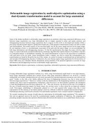
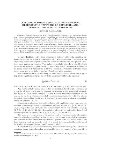
See Figure 1.1 for a simple example. For any itinerary, bifurcation equations will be 

derived for the locus of parameters of all corresponding solutions to (1.1). The idea to 

formulate the unfolding in this way is borrowed from previous studies of heteroclinic 

chains of equilibria [26, 34]. 

Bifurcation studies from heteroclinic chains with equilibria mainly concerned homoclinic 

orbits and generated a huge amount of literature, see, e.g., [6, 10, 14, 16, 26, 

34, 37, 40] just to name a few, and heteroclinic loops between two equilibria, see, e.g., 

[3, 5, 9, 12, 18, 26, 37, 41, 42]. Heteroclinic cycles with periodic orbits have found 

increasing attention recently, see, e.g., [2, 4, 19, 21, 32, 33, 38, 39]. 

The main new contributions of the present work are rigorous results allowing for 

periodic orbits in general heteroclinic networks, for tangent heteroclinic connections, 

and to formulate the bifurcation equations in a general form that can be used as the 

basic building block for a specific study. It is hoped that this makes the results useful 

for readers with applications to specific cases in mind. 

A large field of applications are travelling waves in evolutionary partial differential 

equations in one space dimension whose profiles solve an equation of the form (1.1), 

∗ Centrum Wiskunde en Informatica, Science Park 123, 1098 XG Amsterdam, the Netherlands, 

rademach@cwi.nl [April 27, 2010] 

1

p ∗ 1 

q ∗ 1 

Σ 

p1 

(a) (b) 

Σ 

Σ 

q2 p2 q3 p1 

Fig. 1.1. Sketch of an itinerary for a 2-homoclinic orbit. (a) The homoclinic orbit q∗ 1 (solid) 

and its asymptotic state p∗ 1 at µ = 0, and a 2-homoclinic orbit (dashed). The Poincaré-section 

Σ is just for orientation here. (b) Schematic plot of the itinerary (solid) for a 2-homoclinic orbit 

(dashed) where q2 = q3 = q∗ 1 , p1 = p2 = p∗ 1 . 

but also for instance Laser models are often reduced to this form. There is a very 

large amount of such analytic and numerical studies in the literature, e.g., [8, 19, 22, 

25, 31, 35, 36, 38, 39] to hint at some. 

In the applied literature such bifurcation equations are frequently derived formally 

by a geometric decomposition in terms of local and global maps, e.g., [4, 12, 31]. 

The justification in particular of the local map is an issue and, if linear, requires 

non-resonance conditions on eigenvalues or else dimension dependent normal form 

computations. Other issues are the form of parameter dependence and the persistence 

of solutions upon inclusion of the higher order terms of the original vector field. These 

problems do not arise in the approach taken here, and the results can provide a 

rigourous foundation of formal reductions. 

The reduction to bifurcation equations in this paper is motivated by the so-called 

‘Lin-method’ described in [26], which is a Lyapunov-Schmidt reduction for boundary 

value problems of the itinerary. This method has been used and modified in a number 

of ways and contexts for equilibria, e.g., [17, 16, 40]. Tangent intersection of stable and 

unstable manifolds have been considered mostly for homoclinic orbits, i.e., homoclinic 

tangencies, a paradigm of chaotic dynamics; Lin’s method in this context has been 

used in [16]. Periodic orbits introduce technical complications and for Lin’s method 

these have been overcome in [32] and, using Poincaré-maps, in [33]. Transversality 

studies with respect to parameters in related cases were done in [13]. An ergodic 

theory point of view is taken in [1, 11, 23, 24, 27, 29], and further papers by these 

authors, looking for instance at properties of non-wandering sets. More recently [2] 

treated periodic orbits in a very promising way using Fenichel-coordinates. 

Here [32] is used as a starting point, and equilibria or periodic orbits as vertices 

are treated in an essentially unified manner. Symmetries or conserved quantities are 

not used, but a generic setting is assumed. In contrast to [32], winding numbers of 

heteroclinic sets are not considered, and the underlying heteroclinic network is held 

fixed. Together with [32] this exposition is self-contained, but somewhat technical, 

and parts of [32] have to be repeated and improved in order to track higher order terms 

in this extended setting. The precise statement of the main result Theorem 4.3 can 

only be given rather late after a number of preparatory steps, notation and definitions. 

In particular, this includes §3 where we obtain suitable coordinates near the vertices. 

We next describe the main result, and refer to §5 for sample applications. 

1.1. Description of the main result. For a chosen itinerary the method is 

a Lyapunov-Schmidt reduction which yields algebraic equations that relate system 

parameters µ to certain geometric characteristics Lj, vj at each heteroclinic connection 

qj that the solution follows, perhaps repeatedly, and which connects vertex pj−1 to 

2

pj. The time spent between Poincaré sections Σj−1 at qj−1(0), and Σj at qj(0) is 2Lj 

for Lj ∈ [L ∗ , ∞) if pj is an equilibrium. If pj is a periodic orbit, this time is in general 

only approximately 2Lj since we normalise Lj ∈ {ℓTj/2 : ℓ ∈ N, ℓTj/2 ≥ L ∗ } for the 

minimal period Tj of vertex j. For tangent heteroclinic connections or more than onedimensional 

heteroclinic sets, un/stable manifolds of pj−1 and pj have a more than 

one-dimensional common tangent space at qj(0), and vj are the coordinates on that 

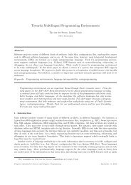
space, except the flow direction. The location of Lj, vj in the itinerary is illustrated 

in Figure 1.2. 

The system parameters µ ∈ R d can generically be assumed to unfold each heteroclinic 

connection by a separate set of parameters µ ∗ j ∈ Rdj which, however, must 

coincide at repeated connections. Here dj is the codimension of the jth connection 

and d = � 

j dj without repeating the same connection in the sum. The geometric 

characteristics couple these parameter sets, but to leading order only to the nearest 

neighbours j ± 1. If dj = 0 for all j, then all heteroclinic connections are transverse, 

and the result proves the existence of solutions for any itinerary, and an expansion 

for the coordinates in the Poincaré-sections. Otherwise, an expansion of µ ∗ j in terms 

of vr, Lr is provided as described next. 

Let κ u/s 

j and σ u/s 

j be the real and imaginary parts of the leading un/stable eigenvalue 

or Floquet exponent at vertex j. For γ ∈ Rr let Cos(γ) = (cos(γ1), . . . , cos(γr)). 

For all j with dj ≥ 1 and for sufficiently large minr{Lr} and small supr{|vr|}, there ex- 

, as well as quadratic 

ist βj, γj ∈ Rdj , and linear maps β ′ j , γ′ j , β′′ j , γ′′ j , ζj, ξj, ζ ′ j , ξ′ j , ζ′′ j , ξ′′ j 

maps Tj (zero if tj = 0), so that a solution follows the chosen itinerary, if and only if 

µ ∗ j = Tj(vj) + e −2κu j Lj Cos(2σ u j Lj + β ∗ j (vj+1, Lj+1))ζ ∗ j (vj+1, Lj+1) 

+e −2κs 

j−1 Lj−1 Cos(2σ s j−1 Lj−1 + γ ∗ j (vj−1, Lj−2)ξ ∗ j (vj−1, Lj−2) + Rj. 

(1.2) 

Here µ ∗ j = µ∗ j ′ whenever the j and j′ in the itinerary correspond to the same actual 

heteroclinic connection. The coupling to the nearest neighbours is given by 

β∗ j (v, L) = βj + β ′ jv + β′′ j Bu j+1 (L), 

γ∗ j (v, L) = γj + γ ′ jv + γ′′ j Bs j−2 (L), 

ζ∗ j (v, L) = ζj + ζ ′ jv + ζ′′ j Bu j+1 (L), 

ξ∗ j (v, L) = ξj + ξ ′ jv + ξ′′ j Bs j−2 (L), 

B s/u 

r (L) = e −2κs/u 

r L Cos(2σ s/u 

r L + β s/u 

r )ζ s/u 

r , 

(1.3) 

where β s/u 

r ∈ Rdr and ζ s/u 

r are linear maps. 

Negative Floquet multipliers, i.e., negative eigenvalues of the period map, have 

Floquet exponent with imaginary part π/Tj. Since L = ℓTj/2, ℓ ∈ N, the argument 

in the cosine terms is πℓ which generates an oscillating sign as ℓ is incremented. 

Note that if the itinerary has repetitions, then vj, Lj have to satisfy solvability 

conditions from repeating the corresponding equations. Each repetition yields new 

parameters vj, Lj, but all other quantities in (1.2) are the same if the underlying 

heteroclinic connections is the same. 

The significance of (1.2) lies in the order of the remainder term Rj, which, for 

certain δ u/s 

j > 0, and arbitrary δ > 0, is given by 

|vj| 3 + e−2κuj Lj 

� 

+e −2κs 

j−1 Lj−1 

e −δu 

j Lj + |vj+1|(e (δ−κu 

j+1 )Lj+1 + |vj+1|) + e (δ−3κu 

j+1 )Lj+1 

� 

e −δs 

j−1 Lj−1 + |vj−1|(e (δ−κs 

j−2 )Lj−2 + |vj−1|) + e (δ−3κs 

j−2 )Lj−2 

3 

� 

� 

.

Σj−2 

µ 

vj−2 

∗ j−2 

2Lj−2 

pj−2 

Σj−1 

µ 

vj−1 

∗ j−1 

2Lj−1 

pj−1 

Σj 

µ ∗ j 

vj 

2Lj 

pj 

Σj+1 

µ 

vj+1 

∗ j+1 

2Lj+1 

pj+1 

Σj+2 

µ 

vj+2 

∗ j+2 

Fig. 1.2. Schematic illustration of an itinerary near index j, and the location of µ ∗ j , vj, Lj. 

The arrows indicate the flow direction, connections can be copies of the same actual heteroclinic 

connection. 

In particular, Rj is higher order with respect to at least one of the cosine terms if 

Lj ∼ Lr, r = j − 1, j − 2, j + 1. 

The application of the above result to a Shil’nikov-homoclinic orbit to an equilibrium 

yields the same bifurcation equations as in [26], and as in that paper, many 

of the seminal results by Shil’nikov [37] follow from leading order analyses. Note that 

the resonant case κ u j = κs j−1 

can be treated by the above result as well. See [6] for 

resonance at homoclinic bifurcations. 

Remark 1.1. Under the ‘flip’ condition Rank(ζj) = 0 or Rank(ξj)j = 0 for 

the leading eigenvalue, the next leading terms need to be taken into account for an 

unfolding. Viewing ζj, ξj as parameters, the bifurcation of solutions can be understood 

from Theorem 4.3 if 2κu j < 2κsj−1 + δs j−1 for ζj = 0 or 2κs j−1 < 2κuj + δu j for ξj = 0. 

To overcome the barriers involving ρs j−1 and ρuj to the next order eigenvalues requires 

a more refined setup beyond the scope of this article. See [34] and also [14, 20, 28] 

for such considerations in case of equilibria applied to homoclinic bifurcations. 

The main result unifies the treatment of equilibria and periodic orbits as vertices 

of a network: for the reduced equations the only difference between equilibria 

and periodic orbits is that Lj is a semi-infinite interval for an equilibrium, but the 

above defined discrete infinite sequence for a periodic orbit. The discrete sequence 

essentially counts the number of rotations that the solution makes about the periodic 

orbit. Note that replacing a periodic orbit by an equilibrium has consequences for the 

codimensions of heteroclinic connections. 

The reduced equations for a specific case can be determined in three steps. First, 

choose the itinerary of the solution type of interest. Second, determine the codimensions, 

including tangencies, of all visited heteroclinic connections. Third, copy the 

equations from Theorem 4.3 for each element in the itinerary with positive codimension, 

and remove geometric characteristics that do not occur according to the type of 

itinerary and tangencies. In case of repetition in the itinerary, the locus of parameter 

values for the solutions should be found by analysing the arising algebraic solvability 

conditions (which can be highly non-trivial). Similarly, in case of tangencies, the locus 

of turning points or folds can be determined. 

To illustrate this and the applicability of the abstract results, some sample applications 

for specific heteroclinic networks are presented in §5. In particular, for a 

generic homoclinic orbit to a periodic orbit conjugacy to (suspended) shift dynamics is 

proven. In addition, equilibrium-to-periodic orbit heteroclinic cycles of various types 

are considered, and 2-homoclinic orbits are studied for the first time in this context. 

Note that the main result separately concerns each solution type as encoded in 

each itinerary. This is suitable, for instance, when looking for the aforementioned 

travelling waves. In some cases a whole class of solutions or even the entire invari- 

4

ant set can be characterised directly. However, our results do not provide stability 

information of the bifurcating solutions or hyperbolicity of invariant sets, or other 

ergodic properties. See [35] for stability results in homoclinic bifurcations using Lin’s 

method (where additionally PDE spectra are considered). As mentioned, the above 

result does not provide an expansion in general in the case of vanishing leading order 

terms (‘flip conditions’). 

This paper is organised as follows. Section 2 contains details about the setting 

and some preparatory results. In §3 a suitable coordinate system is established for 

trajectories that pass near an equilibrium or periodic orbit or lie in un/stable manifolds. 

The main result is formulated and proven in §4. Finally, §5 contains sample 

bifurcation analyses and illustrate how to use the main result. 

Acknowledgement. This research has been supported in part by NWO cluster 

NDNS+. The author thanks Björn Sandstede, Ale Jan Homburg and Alan Champneys 

for helpful discussions. 

2. Setting and Preparation. The basic assumption is that at µ = 0 (1.1) 

possesses a finite heteroclinic network C∗ = (C∗ 1 , C∗ 2 ) with vertices p∗i ∈ C∗ 1 being 

equilibria or periodic orbits, i ∈ I1, and edges q∗ i ∈ C∗ 2 , i ∈ I2, being heteroclinic 

connections. Rather than unfolding C as a whole, we consider the following paths 

within C separately. Here we set Jo := J \ min J (where min J = ∅ if there is no 

minimum). 

Definition 2.1. A possibly infinite set C = ((pj)j∈J, (qj)j∈J o) with pj ∈ C∗ 1, 

j ∈ J and qj ∈ C∗ 2 , j ∈ Jo , is called itinerary if for all j ∈ Jo the edge qj is 

a heteroclinic connection from pj−1 to pj (or homoclinic if pj−1 = pj) and either 

J = {−∞, . . .0, 1}, J = {1, 2, . . . ∞}, J = Z or J = {1, . . .,m} for some m > 1. 

For ease of notation we say that a sequence yj of ‘objects’ (numbers, vectors or 

maps given in the context) with j ∈ Jo has reducible indexing (with respect to C) if 

yj = yj ′ whenever qj = qj ′ for j, j′ ∈ Jo . 

Note that an itinerary can cycle arbitrarily and perhaps infinitely long within the 

heteroclinic network viewed as a directed graph, and the labelling can differ from that 

in C∗ . Any itinerary has a (possibly non-unique) reduced index set Jred ⊂ J so that 

qj �= qj ′ as well as pj �= pj ′ for j �= j′ , with j, j ′ ∈ Jo red := Jred ∩ Jo , and j, j ′ ∈ Jred, 

respectively. Associated to this is Cred = � (pj)j∈Jred , (qj)j∈J o � 

⊂ C, which may not 

red 

itself be an itinerary (though it contains one). 

Let JE ⊂ J be the index set of all equilibria pj in C and JP = J \ JE that of all 

periodic orbits. We set Jo E := JE ∩ Jo and Jo P := JP ∩ Jo . Finally, Tj > 0 denotes the 

minimal period of pj for j ∈ JP, and we set Tj = 0 for j ∈ JE. 

In the following, unless noted otherwise, we consider an arbitrary fixed itinerary 

C. However, until §4 only neighbours qj and qj−1 are relevant. 

For j ∈ J let ˜ Ψj(x, 0) = Aj(x)e Fjx be the Floquet representation of the evolution 

of the linearization ˙v = ∂uf(pj(x); 0)v of (1.1) in pj. Here ˙v = dv/dx, and the 

matrices Aj(x) satisfy Aj(0) = Id, Aj(x + Tj) = Aj(x) for j ∈ JP and x ∈ R, and 

A(x) ≡ Id for j ∈ JE (in which case Fj = ∂uf(pj; 0)). 

The basic assumption about (1.1) and the heteroclinic network is 

Hypothesis 1. The vector field f in (1.1) is of class C k+2 for k ≥ 1 in u and µ. 

The equilibria or periodic orbits p ∗ i , i ∈ I1, are hyperbolic at µ = 0, i.e., for any C the 

matrices Fj have no eigenvalues on the imaginary axis, except for a simple eigenvalue 

at the origin (modulo 2πi) if j ∈ JP. 

5

Here a simple eigenvalue has algebraic and geometric multiplicity one. Hypothesis 

1 implies that the spectrum spec(Fj) of Fj has the un/stable gaps 

κ u j := min {Re(ν) : ν ∈ spec(Fj), Re(ν) > 0} > 0 

κ s j := − max {Re(ν) : ν ∈ spec(Fj), Re(ν) < 0} > 0. 

Since C∗ 1 is finite, the gaps κs/u 

j are uniformly bounded from below in j ∈ J. For 

convenience we choose arbitrary κj > 0, j ∈ J with reducible indexing, such that 

κj < min{κs j , κuj }. We also need the gap to the next leading eigenvalues/Floquet 

exponents. Let νr, r = 1, . . .,n be the eigenvalues of Fj and define 

ρ s j := min{|Re(νr)| − κ s j : Re(νr) < 0, Re(νr) �= κ s j , r = 1 . . .,n}, 

ρ u j := min{Re(νr) − κ u j : Re(νr) > 0, Re(νr) �= κ u j,r = 1 . . . , n}. 

Leading stable eigenvalues of a matrix are those with the largest strictly negative 

real part, and leading unstable those with the smallest strictly positive real part. For 

the main result, we will assume that these leading eigenvalues are simple as expressed 

in the following hypotheses. 

Hypothesis 2. Consider the leading stable eigenvalues or Floquet exponents 

at pj. Assume that this is either a simple real eigenvalue νj or a simple complex 

conjugate pair νj, ¯νj with Im(νj) �= 0. 

Hypothesis 3. Consider the leading unstable eigenvalues or Floquet exponents 

at pj. Assume that this is either a simple real eigenvalue νj or a simple complex 

conjugate pair νj, ¯νj with Im(νj) �= 0. 

To emphasise where these hypotheses enter we will not assume them globally, 

which has the effect that a priori exponential rates for estimates are not κ s/u 

j , but 

κ s/u 

j − δj for an arbitrary δj > 0 due to possible secular growth. In the following 

δj denotes a priori an arbitrarily small positive number, which may vanish under 

Hypothesis 2, 3. 

Hence, for suitable xj ∈ [0, Tj) as well as asymptotic phases αj ∈ [0, Tj) of qj 

with respect to pj we obtain the estimates (see, e.g., [7]) 

(δj −κs 

|qj(x) − pj(x + αj)| ≤ Ce j )x , x ≥ 0 (2.1) 

(δj −κu 

|qj+1(x + xj) − pj(x + αj)| ≤ Ce j )|x| , x ≤ 0, 

where C > 0 depends only on qj, qj+1 and δj. For j ∈ JP the requirement (2.1) of 

equal asymptotic phase for qj(0) and qj+1(xj) determines xj up to multiples of Tj 

and uniquely in [0, Tj). For j ∈ JE we have pj(x) ≡ pj and set αj = xj = 0. 

To distinguish in- and outflow at pj we denote ˆqj(x) := qj+1(x+xj) for j −1 ∈ J o . 

Let Φj(x, y) denote the evolution of ˙v = ∂uf(qj(x); 0)v and ˆ Φj(x, y) that of 

˙v = ∂uf(ˆqj(x); 0)v. Hyperbolicity of pj gives the following exponential dichotomies 

for j ∈ Jo E and trichotomies for j ∈ Jo P (see, e.g., [32]). 

Notation. Indices separated by one or more ‘slashes’ as in κ s/u 

j indicate alternative 

choices for the statement with all these indices chosen equal at a time. 

There exist projections Ψ s/c/u 

j 

in x ≤ 0, such that the following holds. Set Φ s/c/u 

j 

ˆΦ s/c/u 

j 

(x, y) := ˆ Φj(x, y) ˆ Ψ s/c/u 

j (y), respectively. 

(x), continuous in x ≥ 0, and ˆ Ψ s/c/u 

j (x), continuous 

6 

(x, y) := Φj(x, y)Ψ s/c/u 

j 

(y) and

• For j ∈ Jo P : Rg(Ψcj (x)) = span� d 

dxqj(x) � , 

≡ 0, 

• For j ∈ Jo E : Ψcj ≡ ˆ Ψc j 

• The projections are complementary: Ψs j + Ψuj + Ψcj ≡ Id, Ψs (Ψu + Ψc j ) ≡ 0, 

Ψu (Ψs + Ψc j ) ≡ 0, Ψc (Ψs + Ψu j ) ≡ 0; analogous for ˆ Ψ s/c/u 

j , 

• The spaces Rg(Ψs (x)) and Rg( ˆ Ψu (x)) are unique, the spaces Rg(Ψu (x)) and 

Rg( ˆ Ψs (x)) arbitrary complements such that the previous holds, 

• The projections commute with the linear evolution: 

Φ s/c/u 

j (x, y) = Ψ s/c/u 

j (x)Φj(x, y) and ˆ Φ s/c/u 

j (x, y) = ˆ Ψ s/c/u 

j (x) ˆ Φj(x, y), 

• They distinguish un/stable and center direction: there is C > 0 depending 

on δj > 0 and qj, ˆqj such that for all u ∈ Rn |Φ s (δj −κs 

j(x, y)u| ≤ Ce j )|x−y| |u| , x ≥ y ≥ 0, 

|Φ u (δj −κu 

j(x, y)u| ≤ Ce j )|x−y| |u| , y ≥ x ≥ 0, 

|Φ c j (x, y)u| ≤ C|u| , x, y ≥ 0, (2.2) 

| ˆ Φ u j(x, y)u| ≤ Ce (δj −κu j )|x−y| |u| , x ≤ y ≤ 0, 

| ˆ Φ s (δj −κs 

j(x, y)u| ≤ Ce j )|x−y| |u| , y ≤ x ≤ 0, 

| ˆ Φ c j (x, y)u| ≤ C|u| , x, y ≤ 0. 

We denote the un/stable and center spaces, respectively, by 

E u/s/c 

j 

(x) := Rg(Ψ u/s/c 

j 

(x)), Êu/s/c 

j 

(x) := Rg( ˆ Ψ u/s/c 

j (x)). 

Definition 2.2. For a decomposition E ⊕ F = R n we denote by Proj(E, F) : 

R n → R n the unique projection with kernel E and image F. 

In order to link the trichotomies of the in- and outflow near pj, we define 

P s j (L) := Proj(Eu j (L) + Êc j (−L), Ês j (−L)) 

P u j (L) := Proj( Êsc 

j (−L), E u j (L)) 

P c j (L) := Proj(E u j (L) + Ês j(−L), Êc j(−L)). 

We also define the aforementioned sets of travel time parameters 

� 

[L, ∞) for j ∈ JE 

Kj(L) := 

{ℓTj/2 : ℓTj/2 ≥ L, ℓ ∈ N} for j ∈ JP. 

It is shown in [32], Lemma 2, that there is L0 > 0 such that for L ∈ Kj(L0 ) 

the P s/c/u 

j (L) are complementary projections, P c j ≡ 0 for j ∈ Jo E , and the norms 

|P s/c/u 

j (L)| are uniform in L. 

In order to control the leading order terms in the bifurcations equations we make 

the following change of coordinates locally near all pj, j ∈ Jred. In the new ‘straight’ 

coordinates the un/stable manifolds locally coincide with the un/stable eigenspaces 

of the linearization in pj, respectively. For periodic orbits the strong un/stable fibers 

locally coincide with the un/stable eigenspaces. Since these are graphs over the 

eigenspaces and tangent at the equilibrium or periodic orbit this is straightforward. 

See e.g., (3.27) in [34]. However, as in [34] this change of coordinates is an obstacle 

7

to apply the method within the class of semilinear parabolic partial differential equations. 

However, in [2] this problem has been circumvented in a way that should apply 

here as well. 

To emphasise the effect of this coordinate change and to make the notation of 

estimates throughout the text more readable, we define for j ∈ J and any δj > 0, and 

δj = 0 if explicitly mentioned, the terms 

and set Rj = ˆ Rj = 0 for j �∈ J. 

� 

e 

Rj := 

(δj−κj)Lj a priori, 

e (δj−κuj )Lj in straight coordinates, 

� 

e 

ˆRj := 

(δj−κj)Lj a priori, 

e (δj−κs j )Lj in straight coordinates, 

Notation. In the following we use the usual order notation a = O(b) if there 

is a constant C > 0 such that |a| ≤ C|b| for all large or small enough b and norms 

as given in the context. In terms of Lj this is always as Lj → ∞. In a chain 

of inequalities for such order computations we allow the constant C to absorb other 

constant factors and take maximum values of several constants without giving explicit 

notice. 

The next lemma is the basis for estimating error terms in the following sections. 

Lemma 2.3. There exist C > 0 and L1 ≥ L0 depending only on qj, ˆqj and δj 

such that for L,Lj ∈ K(L1 ) the following holds for all j ∈ Jo . 

1. |P cu 

2. 

� 

j (Lj)Ψs j (Lj)| ≤ CRj , |P sc 

j (Lj) ˆ Ψu j (−Lj)| ≤ C ˆ Rj. 

|P cu 

j (Lj)(pj(αj + Lj) − qj(Lj))| ≤ CRj ˆ Rj, 

|P sc 

j (Lj)(pj(αj − Lj) − ˆqj(−Lj))| ≤ CRj ˆ Rj. 

3. The above holds under Hypothesis 2 with δj = 0 in ˆ Rj and under Hypothesis 

3 with δj = 0 in Rj. 

4. Under Hypothesis 2 or 3, respectively, there are vectors v u/s 

j in the leading 

un/stable eigenspaces of Fj such that 

v s j �= 0 ⇔ limsup ln(qj(x))/x = −κ 

x→∞ 

s j, 

v u j 

�= 0 ⇔ limsup 

x→−∞ 

ln(ˆqj(x))/x = κ u j , 

and such that under Hypothesis 2 and for any δs j < min{κsj , ρsj } we have 

ˆΦ s j(0, −L)P s j(L)(pj(αj + L) − qj(L)) = e 2FjL v s j + O(e −2(κs j +δs j )L ), 

and under Hypothesis 3 and for any δu j < min{κuj , ρuj } we have 

Φ u j(0, L)P u j (L)(pj(αj − L) − ˆqj(−L)) = e −2FjL v u j + O(e −2(κu 

j +δu 

j )L ). 

Proof. For readability, we set αj = 0, see (2.1). Let ˜ Ψ s/c/u 

j (x) be the stable/center 

and unstable eigen- or trichotomy projections on the whole real line, x ∈ R, of 

˙v = ∂uf(pj; 0)v, 

8

which trivially exist by the Floquet form. Note that these di/trichotomies differ from 

those of the linearization in qj. 

1. First note that 

� 

Ψs j (L) = Proj(Ecu j (L), Es j (L)) 

P cu 

j (L) = Proj(Ês j (−L), Eu j (L) + Êu j (−L)), 

so that P cu 

j (L)Ψsj (L) is determined by Es j (L) − Ês j (−L). (An appropriate norm 

for estimating this difference goes via suitable bases of these linear spaces.) Since 

for L ∈ Kj(L0 ) it holds that ˜ Ψs j (−L) = ˜ Ψs j (L) for all j ∈ Jo (the projections are 

constant for j ∈ Jo E ) we have 

E s j(L) − Ês j(−L) = E s j(L) − Rg( ˜ Ψ s j(L)) + Rg( ˜ Ψ s j(−L)) − Ês j(−L), 

and we will estimate the two differences on the right hand side separately. 

General perturbation estimates of dichotomies (e.g. Lemma 1.2(i) in [34]) imply 

Ψs j (L) − ˜ Ψs −κs 

j (L) = O(e(δj j )L ) and ˆ Ψu j (−L) − ˜ Ψu −κu 

j (−L) = O(e(δj j )L ). 

Hence, on the one hand Es j (L) − Rg(˜Ψ s j (L)) = O(e(δj −κsj )L ). 

On the other hand we can write 

˜Ψ s j (−L) − ˆ Ψ s j (−L) = Id − ˜ Ψ cu 

j (−L) − (Id − ˆ Ψ cu 

j (−L)) = ˆ Ψ cu 

j (−L) − ˜ Ψ cu 

j (−L), 

and, due to asymptotic phase we have d 

dx ˆqj(−L) − d 

dxpj(−L) = O(e (δj −κuj )L ) in 

−κu 

(−L) = O(e(δj j )L ) and Rg( ˜ Ψs j (L)) − 

the center direction. Therefore, ˜ Ψs j (L) − ˆ Ψs j 

Ês −κu 

j (−L) = O(e(δj j )L ). (And analogously Ψs j (L) − ˜ Ψs −κs 

j (L) = O(e(δj j )L )). 

In combination, since Ês j (−L) ⊂ kerPu j (L) the weak version of the first estimate 

follows. The strong version of this estimate in straight coordinates is a consequence 

of the fact that then Es j (L) = Rg(˜ Ψs j (L)) for all L ≥ L1 for sufficiently large 

L1 ≥ L0 . Hence, for L ≥ L1 we have 

E s j(L) − Ês j(−L) = Rg( ˜ Ψ s j(−L)) − Ês j(−L), 

which implies the stronger estimate. 

The proof of the second estimate is completely analogous. 

2. Since the stable manifold is a (at least) quadratic graph over the stable eigenspace 

for j ∈ JE and center-stable trichotomy space for j ∈ JP at pj we have that 

pj(L) − qj(L) = ˜ Ψ sc 

j (L)(pj(L) − qj(L)) + O((pj(L) − qj(L)) 2 ). 

On the other hand, as in the proof of the previous item, we can replace ˜ Ψs j (L) by 

ˆΨ s j (L) with error of order e(δj−κu j )L . Since Ês j 

cu 

(L) lies in the kernel of Pj (L) and 

pj(L) − qj(L) = O(e (δj−κs j )L ) there are non-negative constants C∗ and C∗ such 

that 

P cu 

j (L)(pj(L) − qj(L)) = P cu 

j (L)˜ Ψ c j (L)(pj(L) − qj(L)) (2.3) 

+O(C∗e (δj−κs 

j −κu 

j )L + C ∗ e 2(δj−κs 

j )L ). 

For j ∈ J o P recall that the asymptotic phase as L → ∞ of qj(L) is that of pj(L), 

hence qj(L) lies in the strong stable fiber with phase L. Strong stable fibers are 

(at least) quadratic graphs over the (strong) stable trichotomy spaces so that 

˜Ψ c j (L)(pj(L) − qj(L)) = O((pj(L) − qj(L)) 2 ) = O(e 2(δj −κs j )L ). 

9

The claimed weak estimate follows from combining this estimate with (2.3). 

The stronger estimate for straight coordinates means C ∗ = 0 in (2.3). Indeed, 

since the strong un/stable fibers and (center) un/stable manifold coincide with 

their tangent spaces at pj the higher order corrections disappear and (2.3) holds 

with C ∗ = 0. 

The estimate for pj(αj − L) − ˆqj(−L) is completely analogous. 

3. For simple eigenvalues or Floquet exponents there is no secular growth so that the 

rates of convergence are in fact the leading rates. 

4. This is a reformulation of results in [32] as follows. 

Concerning the right hand sides without ˆ Φ s j (0, −L) and Φu j 

Lemma 10 in [32] yields the expansions 

P s j (L)(pj(αj + L) − qj(L)) = Aj(L)e FjL ˜v s j 

P u j (L)(pj(αj − L) − ˆqj(−L)) = Aj(−L)e −FjL ˜v u j 

+ O(e−2(κs j +δs j )L ), 

(0, L), respectively, 

+ O(e−2(κu j +δu j )L ), 

for certain ˜v u/s 

j in the leading un/stable eigenspace of Fj. Note that in the present 

case α and v from that Lemma are constant, and L ∈ Kj(L1 ) so that pj(αj +L) = 

pj(αj − L) and Aj(L) = Aj(−L). 

Concerning ˆ Φj(0, −L) and Φu j (0, L), Equation (5.7) in [32] shows that for any v 

there are ˆv u/s in the un/stable eigenspace of Fj such that 

ˆΦ s j (0, −L)v = eFjL Aj(−L) −1 ˆv s + O 

Φ u j(0, L)v = e −FjL Aj(L) −1 ˆv u + O 

� 

e −(κsj +δs j )L� 

, 

� 

e −(κu j +δu j )L� 

. 

Since Aj(L) = Aj(−L) for L ∈ Kj(L 1 ), and these expansions only depend on the 

error to the asymptotic vector fields, combination of this with the previous step 

proves the claim. 

3. Coordinates of trajectories. Following and improving [32], in this section 

we establish a suitable coordinate system for the (n−1)-dimensional set of trajectories 

that pass nearby pj. We consider the difference V = (w, ˆw) between solutions u to 

(1.1) and qj, ˆqj, where u(0) ∼ qj(0) and u(2L) ∼ ˆqj(0). (In this section qj, ˆqj can 

be any orbits that lie in the stable and unstable manifolds of pj, respectively.) We 

determine all such V by an implicit function theorem, where the time shift along a 

trajectory is removed to make V unique. For equilibria this is done in the usual way 

of [26] by imposing certain boundary value data of u in Poincaré sections attached to 

the in- and outflowing solutions qj and ˆqj, and adding a continuous parameter L so 

that 2L is the time spent between the section. 

For periodic orbits it would be natural to do the same, only L would not come 

from a connected unbounded interval in order for V to be small. However, due to our 

approach via a certain variation-of-constants solution operator, we slightly deviate 

from this, see also [32]. Briefly, in order to control the integrals over the centre part 

of the trichotomy projections, we use exponentially weighted spaces. This causes 

difficulty to control the centre projection of another integral term from coupling inand 

outflow, which stems from the deviation of the phase with respect to pj at x = L. 

Due to asymptotic phase this term vanishes in the limit L → ∞, but integrability 

requires a good estimate. We avoid this and at the same time remove the phase shift by 

simply requiring that the centre parts of w(x) and ˆw(ˆx) at time x = L, ˆx = −L vanish. 

10

This precisely disallows time shifts and the result is equivalent to the approach by 

Poincaré sections. In particular, the resulting V give a parameterisation of all orbits 

near pj with normalised travel time sequence. A posteriori, the reconstructed solutions 

approximately satisfy boundary conditions in suitable linear Poincaré sections and 2L 

is the approximate travel time between these. 

Notably, this parametrises trajectories in a neighborhood of {qj(x) : x ≥ 0} ∪ 

{ˆqj(ˆx) : ˆx ≤ 0}. An alternative to this approach is to parametrise trajectories in a 

small neighborhood of pj and then insert a ‘global’ trajectory piece between the inflow 

and outflow boundaries of these neighborhoods, see [2, 4, 37]. 

3.1. Passage coordinates. We choose the boundary value data in subsets of 

Poincaré sections defined via the trichotomies. For j ∈ JP the space (qj(0), ˆqj(0)) + 

Es j (0) × Êu j (0) is (n − 1)-dimensional since the flow direction counts towards stable 

and unstable directions for periodic orbits. On the other hand, for j ∈ Jo E we have 

(x) so that after removing the flow directions for in- and 

˙qj(x) ∈ Es j (x) and ˙ ˆq(x) ∈ Êu j 

outflow n −2 dimensions are left. As mentioned, this is compensated by a continuous 

‘travel time’ parameter L ∈ Kj(L1 ). To eliminate the flow direction for j ∈ Jo E we 

define 

Q s j := Proj � E u j (0) + span( ˙qj(0)), E s j(0) ∩ span( ˙qj(0)) ⊥� , 

� 

s 

:= Proj Êj (0) + span( ˙ ˆqj(0)), E u j (0) ∩ span( ˙ ˆqj(0)) ⊥� 

. 

ˆQ u j 

Here E ⊥ is the orthogonal complement of a linear space E. For the outflow we define 

ˆQ u j accordingly, and set Qs j := ˆ Q u j := Id for j ∈ Jo P . 

Now boundary data in Qs jEs j (0) × ˆ Qu jÊu j (0) for all j ∈ Jo excludes precisely 

the flow directions at qj(0) and ˆqj(0). Recall that Es j (0) and Êu j (0) are determined 

uniquely by the di-/trichotomy. 

Finally, for all j ∈ J we define the Poincaré sections 

Hence, for j ∈ J o E 

Σj := qj(0) + Q s j Es j (0) + Eu j (0), 

ˆΣj := ˆqj(0) + Ês j(0) + ˆ Q u j Êu j (0). 

we solve the boundary value problem (1.1) subject to u(0) ∈ 

there are technical reasons not to 

Σj and u(2L) ∈ ˆ Σj. As mentioned, for j ∈ Jo P 

consider this boundary value problem. In addition, the set of travel times has to be 

‘phase coherent’ in order for the variations V to be small near the periodic orbit. 

For convenience we a priori restrict L to the set Kj(L1 ) which already appeared in 

Lemma 2.3. For general Poincaré sections, the set Kj would need to be adjusted and 

therefore, in general, differs for each µ, which is inconvenient for the leading order 

expansion of parameters. The tradeoff is that orbits starting in Σj do not necessarily 

lie exactly in ˆ Σj for L ∈ Kj(L1 ): instead of having zero center part at time 2L we will 

require this at time L. Since near qj(0) the flow acts as a diffeomorphism between 

any choice of hyperplanes transverse to the flow this is no restriction, but rather a 

normalisation of the discrete travel times. 

Due to the geometric interpretation, we refer to the boundary data as coordinate 

parameters and denote 

Ωj := Q s j Es j (0) × ˆ Q u j Êu j (0), 

11

pj−1 

ω s j 

Σj 

ˆwj { 

ker(P c (L)) 

pj 

} 

wj 

ˆΣj 

ˆqj 

qj 

ˆω u j 

pj+1 

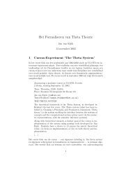
Fig. 3.1. Illustration of the notation for the flow near a periodic orbit pj with minimal period 

Tj, j ∈ JP. Theorem 3.2, see also Corollary 3.3, show that trajectories near {qj(x) : x ≥ 0}∪{ˆqj(ˆx) : 

ˆx ≤ 0} are parametrised by ω s j ∈ Es j (0), ˆωu j ∈ Êu j (0) and L ∈ {ℓTj/2 : ℓ ∈ N, ℓTj/2 ≥ L0}. 

with elements ωj = (ωs j , ˆωu j ) for ωs j ∈ Qsj Es j (0), ˆωj ∈ ˆ Qu jÊu j (0), see Figure 3.1. 

Since we also want to parametrise un/stable manifolds including the flow direction 

for equilibria, we define in addition 

Ω f j := Es j (0) × Êu j (0). 

We now turn to the aforementioned difference V between solutions and heteroclinic 

orbits. Given a solution u for parameters µ we call any 

V (x, ˆx; µ, u, σ, L) := (u(σ + x) − qj(x), u(σ + ˆx + 2L) − ˆqj(ˆx)) 

a j-variation of u and denote the components as V = (w, ˆw). A solution u of (1.1) 

for x ∈ [0, 2L] can be reconstructed from a given j-variation if on the one hand 

for x ∈ [0, L] and ˆx ∈ [−L, 0], where 

d 

dx w(x) = ∂uf(qj(x); 0)w(x) + gj(w(x), x; µ), (3.1) 

d 

dˆx ˆw(ˆx) = ∂uf(ˆqj(ˆx); 0) ˆw(ˆx) + ˆgj( ˆw(ˆx), ˆx; µ), 

gj(w(x), x; µ) := f(qj(x) + w(x); µ) − f(qj(x); 0) − ∂uf(qj(x); 0)w(x), 

ˆgj( ˆw(ˆx), ˆx; µ) := f(ˆqj(ˆx) + ˆw(ˆx); µ) − f(ˆqj(ˆx); 0) − ∂uf(ˆqj(ˆx); 0) ˆw(ˆx). 

On the other hand, the reconstructed orbit is given by 

� 

qj(x) + wj(x) , x ∈ [0, L] 

ˆqj(x − 2L) + ˆwj(x − 2L) , x ∈ [L, 2L] 

and is continuous, if wj(L) − ˆwj(−L) = −qj(L) + ˆqj(−L). Therefore, we define 

bj(L) := ˆqj(−L) − qj(L), 

which will be the main contribution to the expansion given in (1.2). 

We look for solutions that are simultaneously close to qj and ˆqj, so that the 

j-variation V is small and given by an implicit function theorem. Since bj(L) is 

asymptotically periodic for j ∈ Jo P as L → ∞ the aforementioned ‘phase coherence’ 

condition appears, and for L ∈ Kj(L) we indeed have smallness: 

bj(L) = pj(αj + L) − qj(L) + ˆqj(−L) − pj(αj + L) = O(e −κjL ). 

12

Moreover, Lemma 2.3(4) implies for Lj ∈ Kj(L 1 ) that 

The trichotomies imply for x, −ˆx ∈ [0, L] that 

P u j (Lj)bj(Lj) = O(Rj) (3.2) 

P sc 

j (Lj)bj(Lj) = O( ˆ Rj). (3.3) 

R n ∼ E s (x) × E c (x) × E u (x) ∼ Ês (ˆx) × Êc (ˆx) × Êu (ˆx) 

and provide a decomposition w = w s j + wc j + wu j 

ˆw = ˆw s j + ˆwc j + ˆwu j 

into ˆws/c/u 

j 

(ˆx) := ˆ Ψ s/c/u 

j 

into ws/c/u 

j 

(x) := Ψ s/c/u 

j (x)w(x) and 

(ˆx) ˆw(ˆx). We use the analogous superscripts 

for the decomposition of gj and ˆgj. 

Similar to [34], Lemma 3.4, the following estimates hold. We first change coordinates 

and rescale time so that (see [32]) there is ε0 > 0 such that for |µ| ≤ ε0 we have 

pj(x; 0) = pj(x; µ), j ∈ Jred, i.e., pj is independent of µ for |µ| ≤ ε0. 

Lemma 3.1. There is C > 0 depending only on δj and qj, ˆqj such that for 

x, −ˆx ≥ 0, 

� 

|gj(w, x; µ)| ≤ C |w| 2 (δj −κs 

+ |µ|(|w| + e j )x � 

) 

|g s � 

j (w, x; µ)| ≤ C (|w s j | + e(δj−κs j )x )|w| 2 + |µ|(|w s j | + e(δj−κs j )x� 

� 

|ˆgj(w, ˆx; µ)| ≤ C |w| 2 + |µ|(|w| + e (δj −κsj )|ˆx| � 

) 

|ˆg u � 

j ( ˆw, ˆx; µ)| ≤ C (| ˆw u j | + e (δj−κu j )|ˆx| |)| ˆw| 2 + |µ|(| ˆw u j | + e (δj−κu j )|ˆx|� 

(3.4) 

(3.5) 

(3.6) 

(3.7) 

Proof. By definition of straight coordinates, for w ∈ R n , we have ˜ Ψ s j (x)f(pj(x) + 

˜Ψ u j (x)w; 0) ≡ 0, where ˜ Ψ s/c/u 

j 

(x) are the projections of the linear evolution at pj as 

in the proof of Lemma 2.3. From that proof we know Ψ s j (x) − ˜ Ψ s j 

(x) = O(e(δj −κs 

j )x ); 

recall Ψ u/s/c 

j (x) are the projection of the trichotomies Φ(x, y), see (2.2). Therefore, 

Ψ s j (x)f(pj(x) + Ψ u −κs 

j (x)w; 0) = O(e(δj j )x ). 

In the following we omit the argument x for readability and set fs := Ψs j (x)f. Hence, 

We have 

∂uuf s (pj + w; 0) = O(|w s j| + e (δj−κs j )x ). 

gj(w, x; µ) = f(qj + w; µ) − f(qj; 0) − ∂uf(qj; 0)w 

= f(qj + w; µ) − f(qj + w; 0) + f(qj + w; 0) − f(qj; 0) − ∂uf(qj; 0)w 

= 

� 1 

0 

∂µf(q + w; τµ)µdτ + 

� 1 � 1 

0 

0 

∂uuf(q + τsw; 0)τw 2 dτds, 

and ∂µf(pj + w; µ) = O(|w|) since f(pj; µ) = f(pj; 0). It follows that ∂µf = O(|w| + 

e (δj−κs 

j )x ) which proves the first claimed estimate. We also infer ∂µf s = O(|w s | + 

e (δj−κs j )x ) which proves the second claimed estimate. The proof of the remaining 

estimates is completely analogous. 

13

Based on this, V can be found with uniform estimates in L for j ∈ JP in the 

weighted space 

Xη,L = � C 0 ([0, L], R n ) × C 0 ([−L, 0], R n � 

), � · �η,L , 

�(w, ˆw)�η,L = �w� + 

η,L + � ˆw�− η,L , 

�w� + 

η,L = sup{|eηxw(x)| : x ∈ [0, L]}, 

� ˆw� − 

η,L = sup{|eη|ˆx| ˆw(ˆx)| : ˆx ∈ [−L, 0]}. 

By Lemma 3.1, for any 0 ≤ ηj < κj there is a constant C > 0 independent of L 

such that 

� �gj(w, ·; µ, L)� + 

ηj,L 

�ˆgj( ˆw, ·; µ, L)� − 

ηj,L 

≤ C((�w�+ ηj,L )2 + |µ|), 

≤ C((� ˆw�− ηj,L )2 + |µ|). 

(3.8) 

The coordinates of trajectories will be those (ωj, µ, L) with L ∈ Kj(L1), ωj = 

(ω s j , ˆωu j ) ∈ Ωj that generate a fixed point of the map 

Gj(w, ˆw; ωj, µ, L) : Xη,L → Xη,L, j ∈ J o , 

defined next. The maps Gj can be derived from a variation-of-constants solution of 

(3.1) decomposed suitably by the trichotomies and are given by 

⎛ 

⎜ 

� � ⎜ 

x 

⎜ 

Gj(w, ˆw; ωj, µ, L) := ⎜ 

ˆx ⎜ 

⎝ 

Φs j (x, 0)ωs j 

+ � x 

0 Φsj (x, y)gj(w(y), y; µ)dy 

+ � x 

L Φcu 

j (x, y)gj(w(y), y; µ)dy 

+Φ u j (x, L)P u j (L)(cj(L)ω + dj(w, ˆw; µ, L) + bj(L)) 

Φ u j (ˆx, 0)ˆωu j 

+ � ˆx 

−L ˆ Φ sc 

j (ˆx, y)ˆgj( ˆw(y), y; µ)dy 

+ � ˆx 

0 ˆ Φ u j (ˆx, y)ˆgj( ˆw(y), y; µ)dy 

− ˆ Φ sc 

j 

sc (ˆx, −L)Pj (L)(cj(L)ω + dj(w, ˆw; µ, L) + bj(L)) 

where the horizontal line separates first and second component Gj = (Gj,1, Gj,2). The 

terms coupling these components are 

cj(L)ωj = ˆ Φ u j (−L, 0)ˆωu j − Φsj (L, 0)ωs j , 

� −L 

ˆΦ 

0 

u j (−L, y)ˆgj( 

� L 

ˆw(y), y; µ)dy − Φ 

0 

s j (L, y)gj(w(y), y; µ)dy. 

dj(w, ˆw; µ, L) = 

By Lemma 2.3 there is C > 0 depending only on δj and qj, ˆqj such that 

|P u j (L)cj(L)ωj| ≤ C(Rje (δj−κs 

j )L |ω s j| + e (δj−κu 

j )L |ˆω u j |) (3.9) 

|P s j (L)cj(L)ωj| ≤ C(e (δj−κs j )L |ω s j | + ˆ Rje (δj−κu j )L |ˆω u j |). (3.10) 

Note that Ψ c j (L)Gj,1(x = L) = 0 and ˆ Ψ c j (−L)Gj,2(ˆx = −L) = 0. As mentioned 

above, for j ∈ JP, this is equivalent to fixing the phase on a reconstructed orbit from 

a fixed point of Gj. It is shown in [32], Lemma 4, that fixed points of Gj indeed 

generate the aforementioned reconstructed orbits u(x) of (1.1) for x ∈ [0, 2L]. The 

following theorem proves that all orbits can be obtained in this way. Recall that 

14 

⎞ 

⎟ 

⎠

ωj ∈ Ω f j contains the flow direction for j ∈ JE so that the map from fixed points to 

trajectories at x = ˆx = 0 is not injective, while for ωj ∈ Ωj it is. 

Notation. B(X, ρ) := {x ∈ X : |x|X ≤ ρ} where | · |X is the norm of X. 

The following theorem provides the coordinates of trajectories near qj, ˆqj (in fact 

near any in- outflow pair at pj); this is formulated more explicitly in Corollary 3.3 

below. 

Theorem 3.2. Assume Hypothesis 1 and take j ∈ J, as well as any ηj ∈ (0, κj) 

if j ∈ JP, and ηj ∈ [0, κj) if j ∈ JE. There exist ε > 0, L∗ ≥ L1 depending only on 

qj, ˆqj such that the following hold for L ∈ Kj(L∗ ), µ ∈ B(Rd , ε), ωj ∈ B(Ωf j , ε). 

1. There exists a unique Vj = Vj(ωj, µ, L) ∈ Xηj,L such that Vj = Gj(Vj; ωj, µ, L). In 

addition, Vj is Ck smooth in (ωj, µ) and for j ∈ Jo E also Ck smooth in (ωj, µ, L). 

2. Let V (x, ˆx; µ, u, 0, L) = (w(x), ˆw(ˆx)) be the j-variation of a solution u of (1.1) with 

u(0) ∈ Σj and, for j ∈ Jo E , u(2L) ∈ ˆ Σj. If |V (0; µ, u, σ, L)| ≤ ε then there is unique 

σ∗ = O(|P c j (L)w(L; µ, u, σ)|) such that 

for ωj = 

V (·; µ, u, σ ∗ , L) ≡ Vj(ωj, µ, L) 

� 

Q s j Ψs j (0)w(0; µ, u, σ∗ , L), ˆ Q u j ˆ Ψ u j (0) ˆw(0; µ, u, σ∗ , L) 

3. For any δj ∈ (ηj, κj), there is C > 0 such that a fixed point (W, ˆ W)(ωj, µ, L) of 

Gj(·, ωj, µ, L) satisfies, for x, −ˆx ∈ [0, L], 

� 

. 

�W(ωj, µ, L)� + 

ηj,L ≤ C(|µ| + |ωs j | + Rj), 

� ˆ W(ωj, µ, L)� − 

ηj,L ≤ C(|µ| + |ˆωu j | + ˆ Rj), 

|Ψ s (δj −κs 

j(x)Wj(ωj, µ, L)(x)| ≤ Ce j )x , (3.11) 

| ˆ Ψ u j (ˆx) ˆ (δj −κu 

Wj(ωj, µ, L)(ˆx)| ≤ Ce j )ˆx . (3.12) 

4. Under Hypothesis 2 or 3 the estimates (3.11) and (3.12) hold with δj = ηj in ˆ Rj 

or in Rj, respectively. 

Concerning the required smoothness of f, the loss of two degrees of differentiability 

is due to the coordinate changes (which can be performed simultaneously) that 

involve f ′ and that g contains f ′ . 

Before proving this theorem, to emphasise the coordinate system character we 

reformulate part of Theorem 3.2 in the following corollary taking ωj ∈ Ωj. Recall 

from the beginning of this section that then the set of parameters (ωj, L) is (n − 1)dimensional 

for all j ∈ J o . The theorem in particular shows that this is also true for 

the set of fixed points. 

Corollary 3.3. For any j ∈ J o there is ε > 0 and L ∗ ≥ L 1 as well as a 

neighbourhood U of {qj(x) : x ∈ [0, L]} ∪ {ˆqj(x) : x ∈ [−L, 0]} such that the following 

holds. The set of solutions u of (1.1) that lie in U and satisfy u(0) ∈ Σj, and, 

if j ∈ J o E , u(2L) ∈ ˆ Σj for L ∈ Kj(L ∗ ) is in one-to-one correspondence with the 

parameters {(ωj, µ, L) : ωj ∈ B(Ωj, ε), L ∈ Kj(L ∗ ), |µ| ≤ ε} of fixed points of Gj. 

Proof of Theorem 3.2. Items 1 and 2 are a consequence of Theorem 1 in [32] as 

follows. There it was assumed that |µ| ≤ εe −ηjL , but in the present case we can take 

|µ| ≤ ε due to the following estimate. For any 0 < ηj < κj we have 

�∂wgj(w, ·; µ)� + 

+ 

η,L ≤ K1(�w� η,L + |µ|), 

15

and the same with hats in the � · � − 

η,L-norm (see [34] Lemma 3.1). This estimate 

improves the corresponding estimate at the end of the proof of Lemma 5 in [32] as 

needed. All constants are uniform in L ∈ Kj(L∗ ). 

Items 3 and 4 improve the estimate of Theorem 1 in [32] using Lemma 2.3 as 

follows. Theorem 1 in [32] states 

�(Wj, ˆ Wj)�η,L ≤ C(|µ| + |ωj| + e (η−κj)L ), 

where for j ∈ JE we can set η = 0 since there is no centre direction. 

To improve this we consider Wj and ˆ Wj separately and note that the coupling 

of these only enters through dj, while the dependence of Wj on ˆω u j and ˆ Wj on ω s j 

is only by cj. On account of (3.9), (3.10), the decomposition of ω in the claimed 

separate estimates of Wj and ˆ Wj follows. The estimates (3.2), (3.3) prove the claimed 

separation for the remainder term bj(L). Again note that η = 0 is allowed for j ∈ JE. 

It remains to estimate dj and to prove the pointwise estimates for W s j = Φs j W 

and ˆ W u j = ˆ Φ s j ˆ W. We first consider the pointwise estimates. By definition of Gj,1 

W s j (x) = Φsj (x, 0)ωs j + 

� x 

0 

Φ s j (x, y)gj(Wj(y), y; µ)dy, 

and so using (2.2) and (3.5), for a weight η to be determined there is C > 0 such that, 

e ηx |W s � 

j (x)| ≤ C e (η−κs j )x |ω s j | + 

≤ C 

� x 

e 

0 

(η−κs 

+|µ|(|Wj(y)| + e (δj−κsj )y � � 

) dy 

� 

e (η−κs j )x |ω s � x 

j| + e (η−κs 

0 

j )x+κs 

� 

jy (|W s j (y)| + e(δj−κs j )y )|Wj(y)| 2 

j )x+κs j 

y � 

(e −ηy �W s j � + 

η,L 

× e −2ηy (�Wj� + 

η,L )2 + |µ|(e −ηy �W s j �+ 

η,L + e(δj−κs j )y ) 

+ e(δj−κs j )y ) 

� � 

dy . 

Taking maxima over x this implies for any 0 < η < κ s j (and 0 ≤ η < κs j 

that 

�W s j � + 

� 

η,L ≤ C |ω s j| + (1 + �W s j � + + 

η,L )(�Wj� η,L )2 � 

+ |µ| , 

and in particular for any δ > 0 there exists C > 0 such that 

�W s j �+ 

(δ−κ s j ),L ≤ C ⇔ |W s j (x)| ≤ Ce(δ−κs j )x , x ∈ [0, L]. 

for j ∈ JE) 

The estimate for ˆ Wj(x) is completely analogous, only now κu j bounds η. 

We now turn to the required estimate involving dj. Substituting (3.11), (3.12) 

into (3.5) and (3.7) gives C > 0 such that 

|g s � 

j(w, x; µ)| ≤ C e (δj−κsj )x (|w| 2 � 

+ |µ|) 

(3.13) 

|ˆg u � 

j ( ˆw, ˆx; µ)| ≤ C e (δj−κu j )|ˆx| |(| ˆw| 2 � 

+ |µ|) . (3.14) 

16

Concerning dj these estimates yield (suppressing y, µ in ˆgj) 

| 

� −L 

0 

Analogously, 

ˆΦ u j(−L, y)ˆgj( ˆ Wj)dy| ≤ C 

| 

� L 

0 

≤ C( 

≤ C 

� −L 

e 

0 

−κuj (L+y) e (δj−κuj )|y| (| ˆ Wj|(y)| 2 + |µ|)dy 

� −L 

e 

0 

−κuj L e −δj|y| (� ˆ Wj� − 

δ,L )2dy + |µ|) 

� 

e −κu j L (� ˆ Wj� − 

ηj,L )2 � 

+ |µ| . 

Φ s j (L, y)gj(Wj, 

� 

y, µ)dy| ≤ C e −κsj L (�Wj� + 

ηj,L )2 � 

+ |µ| . 

Hence, using Lemma 2.3 there is C > 0 depending on δj > 0 such that 

|P u j (L)dj(Wj, ˆ Wj; L, µ)| ≤ C(Rj(� ˆ Wj� − 

ηj,L )2 + Rj ˆ Rj(�Wj� + 

ηj,L )2 + |µ|), (3.15) 

|P sc 

j (L)dj(Wj, ˆ Wj; L, µ)| ≤ C( ˆ RjRj(� ˆ Wj� − 

ηj,L )2 + ˆ Rj(�Wj� + 

ηj,L )2 + |µ|). (3.16) 

This completes the proof of the claimed estimates. ✷ 

Note that the differences in this result between an equilibrium (j ∈ JE) and a 

periodic orbit (j ∈ JP) are twofold: 

1. The ranges of L values measuring the time spent near pj are a semi-infinite interval 

for j ∈ J o E and a discrete infinite (phase coherent) sequence for j ∈ Jo P , 

2. In the periodic case the exponential weight ηj must be strictly positive. 

3.2. Stable and unstable manifolds. For homoclinic or heteroclinic connections 

it is helpful to parametrise the stable and unstable manifolds of pj in the same 

way as above. This is in fact simpler than the general case and we can set L in the 

definition of Gj to infinity, which gives, for j ∈ Jo , 

⎛ 

⎞ 

G ∞ j (w; ω s j, µ)(x) := 

ˆG ∞ j (w; ˆωu j , µ)(ˆx) := 

⎝ 

⎛ 

⎜ 

⎝ 

Φ s j (x, 0)ωs j 

+ � x 

0 Φsj (x, y)gj(w(y), y; µ)dy 

+ � x 

∞ Φcu j (x, y)gj(w(y), y; µ)dy 

ˆΦ u j (ˆx, 0)ˆωu j 

+ � ˆx 

−∞ ˆ Φ sc 

j (ˆx, y)ˆgj( ˆw(y), y; µ)dy 

+ � ˆx 

0 ˆ Φ u j (ˆx, y)ˆgj( ˆw(y), y; µ)dy 

The same change in the proof of Theorem 3.2 gives the following corollary concerning 

the parametrization of un/stable manifolds Ws/u (pj). 

Corollary 3.4. There exists ε > 0 such that for all (µ, ωj) ∈ Rd ×Ωf j with |µ|+ 

|ωj| ≤ ε the operators G∞ j and ˆ G∞ j have unique Ck smooth fixed points W ∞ j (x; ωs j , µ) 

and ˆ W ∞ j (ˆx; ˆωs j , µ) satisfying the following. 

1. For j ∈ JE the maps ωs j ↦→ W ∞ j (0; ωs j , µ)(0) and ˆωu j ↦→ ˆ W ∞ j (0; ˆωu j , µ)(0) parametrise 

Ws (pj) and Wu (pj) near qj(0) and ˆqj(0) over Es j (0) and Êu j (0), respectively. 

2. For j ∈ JP, α ∈ [0, Tj) the maps ωs j ↦→ W ∞ j (α; ωs j , µ) and ˆωu j ↦→ ˆ W ∞ j (α; ˆωu j , µ) 

parametrise the strong stable and unstable fibers of pj with phase αj +α over Es j (0) 

and Êu j (0), respectively. 

3. Theorem 3.2(3) holds for W ∞ j with Rj = 0 and ˆ W ∞ j with ˆ Rj = 0. 

17 

⎠ 

⎞ 

⎟ 

⎠

Wj−1 

qj−1 

pj−1 

ˆWj−1 

ˆΣj−1 Σj 

ˆqj−1(0) 

Wj 

qj(0) 

pj 

ˆ Wj 

qj+1 

Fig. 4.1. Schematic illustration of adjacent j-variations. 

4. Bifurcation equations. Based on the results of the previous section we 

derive reduced equations whose solutions parametrise all solutions of (1.1) that are 

near the chosen itinerary C. Throughout this section we take ωj = (ωs j , ˆωu j ) ∈ Ωj. 

In order to reconstruct solutions of (1.1) from the variations (Wj, ˆ Wj) about 

adjacent qj these need to fit together continuously. By definition of the variations 

this means solving (up to the flow direction as shown below) the system of equations 

Wj(x = 0; ω s j , ˆωu j , µ, Lj) = ˆ Wj−1(ˆx = 0; ω s j−1 , ˆωu j−1 , µ, Lj−1), (4.1) 

where j ∈ J o . System (4.1) is closed if J = Z, and closing conditions are required for 

J with upper or lower bound. 

In case of finite J reconstructed solutions are either heteroclinic from p1 to pm 

(‘het’ in short) and, for p1 = pm, homoclinic to p1 (‘hom’) or periodic orbits (‘per’). 

Note that the same periodic orbit is a solution for any periodically prolonged itinerary, 

and in this case we implicitly assume C is a heteroclinic cycle. The remaining cases 

are semi-unbounded J for which we require the corresponding solution to lie in the 

un/stable manifold of pj with the largest or smallest index, respectively. 

More formally, this means 

‘het’: q2(0) + W2(0) ∈ W u (p1) and ˆqm−1(0) + ˆ Wm−1(0) ∈ W s (pm), i.e., 

W2(0; ω2, µ, L2) = ˆ W ∞ 1 (α1; ω u 1 , µ), 

ˆWm−1(0; ωm−1, µ, Lm−1) = W ∞ m (αm; ω s m, µ), 

‘hom’: (really the same as ‘het’, here extra only for clarity) 

q2(0) + W2(0) ∈ W u (p1) and ˆqm−1(0) + ˆ Wm−1(0) ∈ W s (p1), i.e., 

W2(0; ω2, µ, L2) = ˆ W ∞ 1 (α1; ω u 1, µ), 

ˆWm−1(0; ωm−1, µ, Lm−1) = W ∞ 1 (α1; ω s 1 , µ), 

‘per’: W1(0; ω1, µ, L1) = ˆ Wm(0; ωm, µ, Lm), 

‘semi-’: ˆq0(0) + ˆ W0(0) ∈ W s (p1), i.e., 

‘semi+’: q2(0) + W2(0) ∈ W u (p1), i.e., 

ˆW0(0; ω0, µ, L0) = W ∞ 1 (α1; ω s 1, µ), 

W2(0; ω2, µ, L2) = ˆ W ∞ 1 (α1; ω u 1 , µ). 

In order to unify notation for these cases, we set L1 = ∞ for ‘semi±’ and L1 = 

Lm = ∞ for ‘het’ and ‘hom’ so that all equations are of the form (4.1). We thus omit 

the superscript ‘∞’ and take indices modulo m + 1 for ‘per’. System (4.1) then needs 

to be solved for j ∈ Jo with the modified definition 

J o ⎧ 

⎪⎨ J mod m + 1 for ‘per’, 

:= J \ {1} for ‘semi−’, ‘hom’ and ‘het’, 

⎪⎩ 

J for ‘semi+’ and when J = Z, 

18

uj 

ˆΣj 

Σj+1 

000000 

111111uj+1 

000000 

111111 

000000 

111111 

000000 

111111 

000000 

111111 

ˆqj(0) 

qj+1(0) 

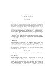
Fig. 4.2. Schematic plot of the flow box near the trajectory between ˆqj(0) and qj+1(0). A left 

orbit uj that enters the box at the same coordinate in ˆΣj as a right orbit uj+1 in Σj+1 lies on the 

same trajectory as uj+1. 

Free travel time parameters are then Lj with j ∈ JL where 

J L � 

J 

:= 

o for ‘semi±’, ‘per’ and if Jo = Z, 

{2, . . .,m − 1} for ‘hom’ and ‘het’. 

The parameters of fixed points of (Gj)j∈J o are thus ωj, j ∈ J o , and Lj, j ∈ J L , and 

the actual system parameters µ ∈ R d . In the Lyapunov-Schmidt reduction we first use 

the coordinate parameters ωj, and then, if needed, express the system parameters µ 

through the time parameters Lj and possibly remaining coordinate parameters. This 

also determines the generic minimum number of parameters needed for the unfolding 

of the part of the network that is visited by the selected itinerary. 

If C contains a sequence of adjacent periodic orbits, the requirement of equal 

asymptotic phase in Theorem 3.2 for in- and outflow at each of these may require 

different qj+1(0) and ˆqj(0), i.e. xj �= 0 in the definition of ˆqj. In that case solving 

(4.1) requires a nontrivial shift in the flow direction. However, this direction is not 

directly available since we removed the flow direction from the coordinate parameters 

ωj. 

To trivialise the matching in this direction we change coordinates locally in a 

neighbourhood of the trajectory segments Yj := {qj(x) : 0 ≤ x ≤ max{Tj, Tj−1}} 

for all j ∈ JP, to obtain ‘flow box’ coordinates so that the flow is parallel to Yj in a 

tube about it, see Figure 4.2. Since C∗ is finite we can choose a uniform tube radius. 

Note that this change of coordinates is independent of the changes near pj performed 

above. 

Remark 4.1. 

1. Since fixed points of Gj are coordinates of trajectories (Corollary 3.3) there is a 

bijection between solutions (up to time shifts) of system (4.1) with all closing conditions 

and solutions of (1.1) that stay in a certain neighbourhood of the itinerary, 

if we require minimal period for periodic solutions. 

2. Due to the flow box coordinates near problematic qj(0), it is in fact not necessary 

to solve (4.1) in the flow direction ˙qj(0): Even if the orbits reconstructed from fixed 

point components Wj of Gj and ˆ Wj−1 of Gj−1 do not fit together in the flow direction, 

a unique trajectory is selected, see also Figure 4.2. Proof: By construction, 

all trajectory segments 

� 

qj(x) + Wj(x), x ∈ [0, Lj] 

uj(x) = 

ˆqj(x − 2Lj) + ˆ Wj(x − 2Lj), x ∈ [Lj, 2Lj], 

j ∈ J L , are continuous at Lj. A priori we would require the jumps uj(2L)−uj+1(0) 

to vanish. However, since the vector field in the flow box is parallel to qj the 

19

coordinates in the un/stable trichotomy spaces E s/u 

j+1 (x) and Ês/u j (x) do not change 

within the flow box. Therefore, the segments uj and uj+1 lie on the same trajectory, 

if and only if their j- and (j + 1)-variations have same coordinates in E s/u 

j+1 (0) and 

Ê s/u 

j (0). 

Recall the spaces of coordinate parameters H s j := Qs j Es j (0) and ˆ H u j := ˆ Q u j Eu j (0), 

and that these do not contain the flow direction. 

To motivate the following definitions, notice that ωs j and ˆωu j−1 explicitly appear 

in (4.1) when substituting the definition of Gj at x = ˆx = 0. In fact, (4.1) projected 

onto Ej := Hs j + ˆ Hu j−1 can be solved using ωj, and we therefore define 

Pj := Proj(E ⊥ j , Ej). 

Lyapunov-Schmidt reduction now consists of solving the system (4.1) projected first 

by Pj and then substituting the result into the projection by Id − Pj. In this process 

the flow direction need not be considered as shown in Remark 4.1. Therefore, the 

directions that are unreachable by coordinate parameters are 

E b j := � E s j (0) + Eu j (0)� ⊥ . 

Hence, dj := dim(Eb j ) is the number of reduced equations at qj(0) that need to be 

solved by system parameters. 

Definition 4.1. Let Jb ⊂ Jo be the set of indices for which dj ≥ 1. 

We set d := � 

j∈Jb ∩Jred dj and will show that this is the number of parameters 

needed to unfold Cred and thus to locate the solutions selected by the choice of C. We 

call additional parameters auxiliary. 

If Hs j ∩ ˆ Hu j−1 is non-trivial, then the representation of RgPj by ωs j + ˆωu j−1 is 

not unique. To make it unique, we remove the intersection from Hs j and denote the 

remaining coordinate parameters by vj ∈ Hs j ∩ ˆ Hu j−1 . More precisely, we define 

˜Pj := Proj([H s j ∩ ˆ H u j−1] ⊥ , H s j ∩ ˆ H u j−1) (4.2) 

˜H s j := ker( ˜ Pj) ∩ H s j , 

so that for ω s j ∈ Hs j there exist unique vj ∈ Rg ˜ Pj and ˜ω s j ∈ ˜ H s j with ωs j = vj + ˜ω s j . 

Definition 4.2. Let J t ⊂ J o be the set of indices for which dim(Rg( ˜Pj)) ≥ 1. 

We denote the collection of all these coordinate parameters by 

� 

¯v = (vj)j∈J t ∈ V := 

j∈J t 

Rg ˜ Pj, 

and endow V with the sup-norm. Parameters vj occur if the tangent spaces of stable 

and unstable manifolds coincide in more than just the flow direction. A transverse 

heteroclinic set of two or more dimensions occurs for j ∈ J t \ J b , which means that 

the ‘linear’ codimension 

n + 1 − dim W s (pj) − dim W u (pj−1) 

is negative and gives the generic dimension of tangency minus the flow direction. 

This only uses information from the un/stable dimensions at the asymptotic states, 

20

pj−1 

W u j−1 

vj 

H s j ∩ ˆ H u j−1 

qj 

W 

pj 

s j 

Fig. 4.3. Illustration of the notation for a tangent heteroclinic connection. 

and tangency of the manifolds may be higher dimensional, and can also occur for 

positive linear codimension. The above defined dj includes this by accounting for the 

, and is always larger than or equal to the linear codimension. 

intersection of Hs j and ˆH u j 

We therefore refer to dj as the codimension of qj. Note that transverse heteroclinic 

connections occur for j ∈ Jo \ Jb and tangent directions transverse to the flow (a 

tangent heteroclinic connection) occurs for j ∈ Jt ∩ Jb , see Figure 4.3. 

To capture the leading order effect of parameter variations on the j-variation we 

define the Melnikov-type integral maps for j ∈ J b 

Mj : R d dj � 

� 

→ Ej , µ ↦→ 

r=1 

〈∂µf(qj(y); 0)µ , aj,r(y)〉dy a 

R 

0 j,r , 

where a 0 j,r ∈ Rn , r = 1, . . . , dj is a basis of E b j with reducible indexing, and aj,r(y) is 

the solution to the adjoint linear equation 

˙a = −∂u(f(qj(y); 0)) t a, 

with a(0) = a 0 j,r . On account of (2.2) Mj is well-defined. 

Note that auxiliary parameters ˜µ lead to a modified map 

(µ, ˜µ) ↦→ Mjµ + ˜ Mj˜µ ∈ E b j . 

The complete Melnikov-map for d parameters is then 

M : R d → Ēb := � 

E b j , µ ↦→ (Mjµ) j∈Jb. (4.3) 

j∈J b 

Hypothesis 4. ker(M) = {0}. 

Repeated elements in C mean repeated rows in M. For an equation Mµ = X this 

means that the solvability conditions on the coordinates Xj of X in Eb j are Xj = Xj ′ 

whenever qj = qj ′, j, j′ ∈ Jb . To solve the remaining part of Mµ = X separately 

in each E b j 

as far as possible we change parameters as follows. Under Hypothesis 4 

the Melnikov map Mred : Rd → � 

j∈Jb ∩Jred Eb j s invertible. Set ˇµ = Mredµ and 

ˇf(u; ˇµ) := f(u; M −1 

redˇµ) and omit the ‘check’ in the following. In the new parameters 

in the sense that 

Mred is the identity on E b j 

dj � 

Mjµ = 

r=1 

µjra 0 j,r , 

for a unique subcollection ¯µj = (µjr)r=1,...,dj of parameters, and µ ∼ = (¯µj) j∈Jred∩J b. 

21

To unify notation of bifurcation equations for parameters and solvability conditions 

we define itinerary parameters µ ∗ j for all j ∈ Jb as follows. Set µ ∗ j = ¯µj for 

j ∈ Jred ∩ J b and, for j ∈ J b \ Jred, µ ∗ j = ¯µj ′ whenever j′ ∈ J b is such that qj = qj ′. 

Due to the above change of parameters, solutions to Mjµ = X can be cast simply as 

µ ∗ j = Xj, j ∈ J b . 

In preparation of the main theorem statement we define for j ∈ J b ∩ J t the map 

dj � 

� 

Tj(vj) := − 

r=1 

〈∂uuf(qj(y); 0)(Φ 

R 

∗ j(y)vj) 2 , aj,r(y)〉dy a 0 j,r, 

which measures the quadratic separation of the tangent manifolds by vj ∈ Rg( ˜ Pj) 

and 

Φ ∗ � 

Φ 

j(y) := 

s j (y), y > 0 

ˆΦ u j−1 (y), y ≤ 0. 

On account of (2.2) Tj(vj) is well-defined and Tj(vj) = O(|vj| 2 ). The following terms 

will capture the leading order effect of the neighbouring itinerary elements and give 

rise to the expansion of the bifurcation equations. 

From (2.2), (3.2) and (3.3) we infer 

B u j (Lj) := Φ u j(0, Lj)P u j (Lj)bj(Lj), 

B s j(Lj) := ˆ Φ s j(0, −Lj)P s j (Lj)bj(Lj). 

|B u j (Lj)| = O(e (δ−κu 

j )Lj Rj) = O(R 2 j), (4.4) 

|B s j (Lj)| = O(e (δ−κs j )Lj ˆ Rj) = O( ˆ R 2 j ). (4.5) 

The following hypothesis concerns intersections of the heteroclinic orbits and the 

spaces Eb j as well as Ej with leading un/stable fibers and trichotomy spaces, respectively, 

and excludes flip bifurcations. 

Hypothesis 5. Let ν s/u 

j be the leading stable/unstable eigenvalues or Floquet 

exponents at pj with Im(ν s/u 

j ) ∈ [0, 2π), and κ s/u 

j := Re(ν s/u 

j ). 

ln(ˆqj(x)) 

1. limsup = κ 

x→−∞ x 

u j, 

ln(qj−1(x)) 

2. limsup = κ 

x→∞ −x 

s j−1, 

3. ∃ru ln(aj,r 

∈ {1, . . .,dj} such that limsup 

x→∞ 

u(x)) 

= ν 

−x 

u j , 

4. ∃rs ln(aj,r 

∈ {1, . . ., dj} such that limsup 

x→−∞ 

s(x)) 

= ν 

x 

s j−1, 

ln(Φ 

5. ∃v ∈ Ej such that limsup 

x→∞ 

u j (x, 0)v) 

= ν 

x 

u j , 

ln( 

6. ∃v ∈ Ej such that limsup 

x→−∞ 

ˆ Φs j (x, 0)v) 

= ν 

−x 

s j−1 . 

22

To emphasise the local coupling in the itinerary and to show conjugacy to symbolic 

dynamical systems, see §5.2.2, for an arbitrary 0 < λ < 1, we use the weighted norm 

�¯ L�L := � 

λ j |Lj| (4.6) 

j∈J L 

on the space L(L∗ ) := � 

r∈JL Kr(L∗ ) of the sequence of travel time parameters Lj. 

with the 

In the precise formulation of the main result given next, we identify E b j 

isomorphic Rdj and for j ∈ Jb the following denote linear maps, where M ⊂ Rdj×dj are diagonal matrices. 

β ′ j : Rg( ˜ Pj+1) → Rdj , γ ′ j : Rg( ˜ Pj−1) → Rdj , 

β ′′ 

j : Eu j+1 (0) → Rdj , γ ′′ 

j : Ês j−2 (0) → Rdj , 

ζj, ξj ∈ M, ζ ′ j : Rg( ˜ Pj+1) → M, ξ ′ j : Rg( ˜ Pj−1) → M, 

ζ ′′ 

j : Eu j+1 

Here ker(β ′′ 

j 

(0) → M, ξ′′ 

j : Ês j−2 

(0) → M. 

j ) ⊃ kerPj+1, ker(γ ′′ 

), ker(ξ′′ 

j ) ⊃ kerPb j−1 

so β′′ 

j Pj+1 = β ′′ 

j etc. 

), ker(ζ′′ 

j 

Let ¯ R = (Rj) j∈Jb, and Cos(β) = (cos(β1), . . . , cos(βr)) for β ∈ Rr . 

Finally, ω = (ωj)j∈J o, ˜ω = (˜ωs , ˆω u ) ∈ ˜ Ω := � 

j∈Jo( ˜ Hs j × ˆ Hu � 

j−1 ), and Ē : j∈Jo Ej, 

where ˜ Ω and Ē are endowed with the sup-norm. 

Recall that Lj = ∞, if j �∈ JL and vj = 0 if j �∈ Jt . Similarly, we make the 

convention that a quantity vanishes if its label is outside its range. 

Theorem 4.3. Under Hypotheses 1 and 4, for a given itinerary C with closing 

conditions, if required, there exist L∗ , ε∗, ε∗ > 0 depending only on Cred so that for all 

δ > 0 the following hold. 

1. For all j ∈ Jb assume Hypothesis 2 and 3 at pr for r = j, j ± 1, j − 2 with 

leading un/stable eigenvalues ν u/s 

r = −κ u/s 

r + iσ u/s 

r , respectively. Take any δ s j−1 < 

min{κ s j−1 , κu j−1 , ρs j−1 } and δu j < min{κu j , κs j , ρu j }. For r = j, j ± 1, j − 2 set δr = 0 

if r ∈ Jb ∩ JE and otherwise δr = δ. 

There exists unique βj, γj ∈ Rdj and β ′ j , β′′ j , γ′ j , γ′′ j , ζj, ξj, ζ ′ j , ξ′ j 

, ζ′′ j , ξ′′ j as above, 

as well as unique C k smooth (µ, ˜ω s , ˆω u , ¯ R) : B(V, ε∗)×L(L ∗ ) → B(R d × ˜ Ω× Ēb , ε ∗ ) 

such that (µ, ˜ω s + ¯v, ˆω u ) solves (4.1) for j ∈ J o if and only if µ ∗ j (¯v, ¯ L) satisfy (1.2) 

with (1.3) for j ∈ Jb . All quantities except (¯v, ¯ L) have reducible indexing and 

� 

Rj = O |vj| 3 + e −2κu j Lj 

� 

e −δu j Lj + |vj+1|(Rj+1 + |vj+1|) + R 3 � 

j+1 

+e −2κsj−1 Lj−1 

� 

e −δs j−1Lj−1 + |vj−1|(Rj−1 + |vj−1|) + ˆ R 3 �� 

j−2 , 

d 

dvj 

Rj = O(e −(2κu j +δu j )Lj + e −(2κs j−1 +δs j−1 )Lj−1 + |vj| 2 ). 

Finally, Rank(ζj) ≥ 1 under Hypotheses 5(1) and (3), Rank(ξj) ≥ 1 under Hypotheses 

5(2) and (4). The analogous statement holds for ζu j+1 , ζs j−2 . 

2. For j ∈ Jo , δj = δ and ηj as in Theorem 3.2, and ¯ R = � 

i∈Jb ˆRi−1 + Ri 

∩Jred 

solutions to (4.1) with |(µ, ω)| ≤ ε∗ and | ¯ L| ≥ L∗ satisfy 

�Wj(¯v, ¯ L)� + 

ηj,Lj = O(|vj| + Rj + |¯v| 2 + ¯ R 2 ), 

� ˆ Wj(¯v, ¯ L)� − 

ηj,Lj = O(|vj| + ˆ Rj + |¯v| 2 + ¯ R 2 ). 

If j ∈ JE, then under Hypotheses 2 and 3 at pj we can take δj = 0 in Rj and ˆ Rj. 

23

3. There exists a neighbourhood U of ∪j∈J o red {qj(x) : x ∈ R} such that the set of ( ¯ L, ¯v), 

|¯v| ≤ ε∗, ¯ L ∈ L(L ∗ ) for which there is a solution to (4.1) with |µ| ≤ ε∗ is bijective 

to the following set of (µ, u) ∈ B(R d , ε∗)×C 0 (R, R n ): u solves (1.1) with u(0) ∈ Σ1 

and u(x) ∈ U for all x ∈ R, and there exists (xj)j∈J o ⊂ [0, Tu) with xj+1 − xj > 0 

minimal such that u(xj) ∈ Σj, where Tu ∈ R ∪ {∞} is the minimal period of u. 

In §5 the use of this somewhat abstract result for concrete cases is illustrated by 

a number of examples. See §1.1 for a discussion of Theorem 4.3. 

The remainder of this section is devoted to the proof of Theorem 4.3, which 

proceeds in the two Lyapunov-Schmidt reduction steps 1. solve (4.1) by the coordinate 

parameters ωj, 2. solve the remaining equations except the flow direction by system 

parameters µ. 

4.1. Solvability by coordinate parameters. 

In Ej, the leading order dependence on µ will stem from 

� 

Mj µ := 

which is well-defined due to (2.2) for ˜ Φj = 

R 

˜Φj(y)∂µf(qj(y); 0)µdy, 

� 

PjΦu j (0, y) , y ≥ 0, 

Pj ˆ Φs j−1 (0, y) , y ≤ 0. 

Lemma 4.4. There are C, L ∗ , ε1, ε2, ε3 > 0 depending only on Cred and δj such 

that there exist unique C k smooth (˜ω s , ˆω u , ¯ R)(¯v, ¯ L, µ), (˜ω s , ˆω u , ¯ R) : B(V, ε1)× ¯ L(L ∗ )× 

B(Rd , ε2) → ˜ Ω × Ē, that satisfy, for j ∈ Jo , 

� 

1. Pj 

Wj(0; ˜ω s j + vj, ˆω u j , µ, Lj) − ˆ Wj−1(0; ˜ω s j−1 + vj−1, ˆω u j−1 

2. |˜ω s j | + |ˆωu j−1 − vj| ≤ C 

� 

|µ| + |vj| 2 + R2 j + ˆ R2 � 

j−1 , 

3. ˜ω s j − ˆωu j−1 = −vj + M j µ − B u j (Lj) − B s j−1 (Lj−1) + Rj,1, where 

� 

, µ, Lj−1) = 0, 

� 

Rj,1 = O R 3 j + ˆ R 3 j−1 + (Rj + ˆ Rj−1 + |vj| + |µ|)|µ| + |vj|( ˆ � 

Rj−1 + Rj + |vj|) . 

4. For any solution of (4.1) multiplied by Pj that has |µ| ≤ ε2 and |ω| ≤ ε3 there 

exists unique (¯v, ¯ L) such that ω = (˜ω s (¯v, ¯ L, µ) + ¯v, ˆω u (¯v, ¯ L, µ)). 

Note that M j , B u j , Bs j−1 

have reducible indexing. 

Proof. For j ∈ J o we need to solve 

Pj 

� 

Gj,1(Wj, ˆ Wj; ωj, µ, Lj)(0) − Gj−1,2(Wj−1, ˆ � 

Wj−1; ωj−1, µ, Lj−1)(0) = 0. 

Let vj ∈ Rg( ˜ Pj) and ˜ω s j ∈ ˜ E s j for the decomposition of ωs j = ˜ωs j + vj. Reordering 

terms, using Rg(Pj) = Ej, and that the center direction lies in the kernel of Pj this 

equation becomes 

˜ω s j − ˆωu j−1 = −vj + Rj,2 − B u j (Lj) − B s j−1 (Lj−1), (4.7) 

24

where 

Rj,2 = −Pj 

+Pj 

� 0 

Φ u j (0, y)gj(Wj(y), y; µ)dy (4.8) 

Lj 

� 0 

−Lj−1 

ˆΦ s j−1 (0, y)ˆgj−1( ˆ Wj−1(y), y; µ)dy (4.9) 

−PjΦ u j(0, Lj)P u j (Lj)cj(Lj)ωj 

(4.10) 

−PjΦ u j(0, Lj)P u j (Lj)dj(Wj, ˆ Wj; µ, Lj) (4.11) 

−Pj ˆ Φ s j−1 (0, −Lj−1)P s j−1 (Lj−1)cj−1(Lj−1)ωj−1 

(4.12) 

−Pj ˆ Φ s j−1 (0, −Lj−1)P s j−1 (Lj−1)dj−1(Wj−1, ˆ Wj−1; µ, Lj−1). (4.13) 

By construction, the left hand side of (4.7) is invertible as a map from ˜ Es j (0) × 

Êu j−1 (0) to Ej. We will next estimate the terms in Rj,2 and show that the right hand 

side is a perturbation. 

Note that for r = j − 1, j the terms Wr and ˆ Wr depend on ωr as in Theorem 3.2. 

In particular, the right hand side of (4.7) depends on ˜ω s j−1 and vj−1 (through ωj−1 

which involves ωs j−1 ) as well as ˜ωs j+1 and vj+1 (through ωj which involves ˆω u j ) so that 

each equation is coupled to its left and right neighbour in the itinerary. 

Step 1: estimating (4.8) and (4.9). 

We expand (4.8) and (4.9), and determine the difference to M j µ. As a shorthand 

we use fj = f(qj; 0). Upon expanding gj in w and µ the terms fj and ∂ufjWj cancel; 

similarly for ˆgj−1. Thus, (4.8) and (4.9), respectively, equal 

where 

� 0 

Pj Φ u j (0, y)(∂uufjW 2 j + ∂µfjµ)dy + Rj,3, (4.14) 

−Pj 

Lj 

� 0 

−Lj−1 

ˆΦ s j−1 (0, y)(∂uufj ˆ W 2 j−1 + ∂µfjµ)dy + Rj,4, (4.15) 

Rj,3 = O(|µ| 2 + |µ|�Wj� + + 

+ (�Wj� ηj,Lj ηj,Lj )3 ), 

Rj,4 = O(|µ| 2 + |µ|� ˆ Wj−1� − 

ηj−1,Lj−1 + (� ˆ Wj−1� − 

ηj−1,Lj−1 )3 ). 

The estimates in Theorem 3.2 imply 

Rj,3 = O(|µ| 2 + |ω s j| 3 + R 3 j + (|ω s j| + Rj)|µ|), 

Rj,4 = O(|µ| 2 + |ˆω u j | 3 + ˆ R 3 j−1 + (|ˆω s j| + ˆ Rj−1)|µ|). 

In the following, the estimates of Theorem 3.2 will be substituted directly without 

mentioning. 

We next estimate the term in (4.14) involving ∂uufjW 2 j . Since Wj is a fixed point 

of Gj,1 we have 

Wj(y) = Φ s j(y, 0)ω s j + Φ u j(y, Lj)P u j (Lj)[bj(Lj) + Rj,5] + Rj,6. (4.16) 

Looking at the definition of Gj,1, the remainder term Rj,6 consists of the integrals 

involving gj, while Rj,5 contains the terms involving cj as well as dj. 

25

When estimating the order of Rj,6, (2.2) and the weight ηj allow to ignore the 

integrals and Φu j (x, Lj) in the sense that the integrals are of order �gj� + 

. This is 

ηj,Lj 

estimated in (3.8) to be of order |µ| + |ωs j |2 + R2 j . Concerning Rj,5, (3.9) and (3.15) 

show that Rj,5 = O(Rj). 

In order to get good estimates of the other terms in (4.16) we decompose 

∂uufj(Wj − Φ s j (y, 0)ωs j + Φs j (y, 0)ωs j )2 = ∂uufj(Wj − Φ s j (y, 0)ωs j )2 

+2∂uufj[Wj, Φ s j (y, 0)ωs j ] − ∂uufj(Φ s j (y, 0)ωs j )2 , 

and substitute this into (4.14). Consider X = � 0 

and substitute (4.16) for Wj. Using (2.2), (3.2) as well as Rj,5 = O(Rj) we find 

� 0 

|X| ≤ C 

≤ C( 

Lj 

� 0 

Lj 

(4.17) 

Lj Φu j (0, y)∂uufj(Wj −Φ s j (y, 0)ωs j )2 dy, 

e −κu j y � 

|∂uufj| e −κu j (Lj−y) |P u j (Lj)|Rj 

�2 + |Rj,6| dy 

e −κu 

j (y+2Lj−2y) dyR 2 j + |Rj,6| 2 ) 

≤ C(R 3 j + |µ|2 + |ω s j |4 ). (4.18) 

The remaining terms from (4.17) are directly estimated to be of the order |ωs j |2 and 

�Wj� + 

η,Lj |ωs j |, i.e., of order |ωs j |(|µ| + |ωs j | + Rj). 

where 

In summary, including Rj,3, the term (4.8) can be written as 

−Pj 

� 0 

Lj 

Φ u j(0, y)∂µfjµdy + Rj,7, 

Rj,7 = O � |µ|(|µ| + |ω s j | + Rj) + |ω s j |2 + Rj|ω s j | + R3 � 

j . 

The completely analogous computation for ˆ Wj−1 and (4.9) shows that (4.9) equals 

where 

−Pj 

� 0 

Lj−1 

ˆΦ s j−1(0, y)∂µfjµdy + Rj,8, 

� 

Rj,8 = O |µ|(|µ| + |ˆω u j−1 | + ˆ Rj−1) + |ˆω u j−1 |2 + ˆ Rj−1|ˆω u j−1 | + ˆ R 3 � 

j−1 . 

Letting the bounds in these integrals tend to infinity generates an error of order 

(Rj + ˆ Rj−1)|µ|. Hence, the sum of (4.8) and (4.9) is of the form 

Step 2: Estimate (4.10)-(4.13). 

Using (3.15) and (2.2) shows that (4.11) is of order 

R 2 j 

M j µ + O(Rj,7 + Rj,8). (4.19) 

� 

|ˆω u j | 2 + ˆ Rj|ω s j| 2 + ˆ RjR 2 j + ˆ R 2 � 

j + Rj|µ|, (4.20) 

26

and similarly (3.16) implies (4.13) is of order 

� 

|ω s j−1 |2 + R 2 j−1 + Rj−1 ˆ R 2 j−1 + Rj−1|ˆω u j−1 |2� + ˆ Rj−1|µ|. (4.21) 

ˆR 2 j−1 

By (3.9) it follows that (4.10) is of order 

� 

|ˆω u j | + ˆ Rj|ω s � 

j| , (4.22) 

R 2 j 

and by (3.16) it follows that (4.12) is of order 

� 

Rj−1|ˆω u j−1 | + |ωs j−1 |� . (4.23) 

ˆR 2 j−1 

In summary, Rj,2 = Mj µ + O(Rj,7 + Rj,8 + R2 j |ˆωu j | + ˆR 2 j−1 |ωs j−1 |), and in particular, 

using (4.4) and (4.5), the right hand side of (4.7) is of the form 

−vj + O 

� 

|vj| 2 + R 2 j + ˆ R 2 j−1 + |µ| + |ωs j |2 + |ˆω u j−1 |2 � 

) 

(4.24) 

Step 3: Apply the implicit function theorem. 

On account of (4.24) the right hand side is a perturbation of the invertible left 

hand side for large Lj and Lj−1 and small |vj|. Notably, the constants in the above 

order estimates all depend only on C from Theorem 3.2 and are uniform in Lj, Lj−1. 

Hence, for finite J and any closing condition there are ε1, ε2 and L∗ such that 

the implicit function theorem immediately applies to the then finite system (4.7) for 

and, due to (4.24), there is 

j ∈ J o . This gives unique C k smooth solutions ˜ω s j , ˆωu j−1 

C > 0 such that these satisfy 

|˜ω s j | + | ˆwu j−1 − vj| ≤ C 

� 

|µ| + |vj| 2 + R 2 j + ˆ R 2 � 

j−1 . 

Since ¯ R is a function of ˜ω, ¯v, ¯ L, µ this proves items 1 and 2 of the lemma. Item 3 

follows from the above form of Rj,2, and item 4 from this and the implicit function 

theorem. 

For infinite J the inverse of the map generating the left hand side of (4.7), 

˜Ω → � 

j∈J o 

( ˜ H s j + ˆ H u j−1), (˜ω s j, ˆω u j−1) ↦→ ˜ω s j − ˆω u j−1, 

is given componentwise by ( ¯ Pj, ( ¯ Pj − Id)) with norm measured by that of ¯ Pj := 

Proj( ˜ H s j , ˆ H u j−1 ). Since Cred is finite, this is uniformly bounded in j. The estimates 

of the right hand side of (4.7) and that this involves only j and j − 1 immediately 

gives continuity in ¯ L, ˜ω, ¯v in the spaces L, ˜ Ω, V. Smoothness of order k follows again 

using that (4.7) is local in the index j; smoothness in µ is straightforward. Hence, 

the implicit function theorem applies as in the finite case. 

4.2. Completing the solution using system parameters. Upon substituting 

the solutions ˜ω s j , ˆωu j−1 , j ∈ Jo , from Lemma 4.4 into the fixed points Wj, ˆ Wj of 

Theorem 3.2 the remaining parameters are ¯v, µ and ¯ L. 

As explained in Remark 4.1, the projection of (4.1) to the flow direction ˙qj(0) 

is trivially solved. Therefore, the spaces E b j ⊂ kerPj identify the remaining socalled 

bifurcation equations that determine µ via (4.1) multiplied by all a 0 j,r , j ∈ Jb , 

r ∈ {1, . . .,dj}, which yields 

� 

r=1,...,dj 

〈(Wj − ˆ Wj−1)(0; ¯v, ¯ L, µ), a 0 j,r 〉a0 j,r 

27 

= 0. (4.25)

Recall that a 0 j,r form a basis of Eb j 

so that each summand has to vanish. 

We will show that the boundary terms bj enter the j-th bifurcation equation via 

ˆBj,r(L) := 〈B s j(L), a 0 j+1,r〉, 

Bj,r(L) := 〈B u j (L), a 0 j,r〉, 

Bj(Lj−1, Lj) = � 

r=1,...,dj 

( ˆ Bj−1,r(Lj−1) + Bj,r(Lj))a 0 j,r. 

To capture the leading order dependence of the j-th bifurcation equation on the 

neighbouring (j ± 1)-st we define (recall ¯ Pj from the proof of Lemma 4.4) 

Gj := ¯ Pj+1(vj+1 + B u j+1 (Lj+1) + B s j (Lj)) 

ˆGj−1 := vj−1 + (Id − ¯ Pj−1)(B u j (Lj) + B s j−1 (Lj−1)), 

S + 

j,r := −〈Φu j(0, Lj)P u j (Lj) ˆ Φ u j(−Lj, 0)Gj, a 0 j,r〉dy, 

S − j,r := 〈ˆ Φ s j−1 (0, −Lj−1)P s j−1 (Lj−1)Φ s j−1 (Lj−1, 0) ˆ Gj−1, a 0 j,r 〉dy, 

Sj = Sj(vj+1, vj−1, Lj, Lj−1, Lj+1) := � 

r=1,...,dj 

(S − 

j,r + S+ j,r )a0j,r. Note how in these terms the coordinate parameters vj±1 are transported by the linear 

evolution from qj±1(0) to qj(0), respectively. 

The estimates (2.2), (4.4) and (4.5) imply 

Bj(Lj−1, Lj) = O( ˆ R 2 j−1 + R2 j ), (4.26) 

S + 

j,r = O(R2 j(|vj+1| + R 2 j+1 + ˆ R 2 j)), (4.27) 

S − j,r = O( ˆ R 2 j−1 (|vj−1| + R 2 j + ˆ R 2 j−1 )). (4.28) 

In the following lemma a subtlety for the correction δj in the error terms Rj, ˆ Rj 

arises. For simple leading eigenvalues δj = 0 is possible everywhere, except in the 

estimates of Theorem 3.2 for j ∈ JP, which requires an exponential weight ηj > 0. So 

far this was irrelevant, but now it becomes important, and therefore we let R j = Rj, 

ˆR j = ˆ Rj denote error terms where δj can be set to zero for simple leading eigenvalues. 

Lemma 4.5. 

1. For j ∈ J b and ¯ L, ¯v as in Lemma 4.4, equation (4.25) is of the form 

Mjµ = Tj(vj) − Bj(Lj−1, Lj) + Sj(vj+1, vj−1, Lj, Lj−1, Lj+1) + Rj,9 + Rj,10 

where the remainder terms are Ck smooth and 

� 

Rj,9 = O |µ|(Rj + ˆ � 

Rj−1 + |vj| + |µ|) , 

� � 

Rj,10 = O |vj| |vj| 2 + R 2 j ˆ Rj + ˆ R 2 � 

j−1Rj−1 

+ |vj+1|R 2 j( ˆ Rj + Rj+1 + |vj+1|) + |vj−1| ˆ R 2 j−1( ˆ Rj−2 + Rj−1 + |vj−1|) 

+R 2 j (Rj + ˆ R 2 j + R3 j+1 ) + ˆ R 2 

j−1 ( ˆ Rj−1 + R 2 j−1 + ˆ R 3 j−2 ) 

2. Under Hypothesis 4, for sufficiently small |µ|, |¯v| and large ¯ L, there exist 

unique C k smooth Rj,11 of the same order as Rj,10 such that (4.25) is solved 

if and only if for j ∈ J b the itinerary parameters µ ∗ j satisfy 

µ ∗ j = Tj(vj) − Bj(Lj−1, Lj) + Sj(vj+1, vj−1, Lj, Lj−1, Lj+1) + Rj,11. 

28 

� 

.

Here, Mj, Tj, Bj, Sj have reducible indexing (they do not differ on repeated parts 

of the heteroclinic network in the itinerary). 

Proof. Substituting the definition of Gj, and suppressing some variables for readability, 

the summands in (4.25) are 

−〈Φ u j (0, Lj)P u j (Lj)bj + ˆ Φ s j−1 (0, −Lj−1)P s j−1 (Lj−1)bj−1, a 0 j,r 〉 (4.29) 

� 0 

−〈 

−〈Φ u j(0, Lj)P u j (Lj)cj, a 0 j,r〉 (4.30) 

−〈Φ u j(0, Lj)P u j (Lj)dj, a 0 j,r〉 (4.31) 

−〈 ˆ Φ s j−1 (0, −Lj−1)P s j−1 (Lj−1)cj−1, a 0 j,r 〉 (4.32) 

−〈 ˆ Φ s j−1(0, −Lj−1)P s j−1(Lj−1)dj−1, a 0 j,r〉 

� 0 

(4.33) 

Φ s j(0, y)gj(Wj, y; µ)dy, a 0 j,r〉 (4.34) 

−Lj−1 

+〈 

Lj 

ˆΦ s j−1 (0, y)ˆgj−1( ˆ Wj−1, y; µ)dy, a 0 j,r 〉 (4.35) 

Note first that term (4.29) is precisely − ˆ Bj−1,r(Lj−1) − Bj,r(Lj). 

Step 1: Estimate (4.30)–(4.33). 

From the estimate (4.20) of (4.11) and Lemma 4.4(2) we infer that (4.31) is of 

the order 

R 2 j 

� 

ˆR 2 j + |vj+1| 2 + R 4 j+1 + ˆRjR 2 j + ˆRj(|vj| 2 + R 4 j + ˆR 4 j−1 ) 

� 

+ Rj|µ|. 

Similarly, now using (4.21), (4.33) is of theorder 

� 

R 2 j−1 + |vj−1| 2 + ˆ R 4 j−2 + Rj−1 ˆ R 2 j−1 + Rj−1(|vj| 2 + R 4 j + ˆ R 4 j−1 ) 

� 

+ ˆ Rj−1|µ|. 

ˆR 2 j−1 

Substituting the expansion of ˆω u j 

as well as Lemma 4.4(2) for |˜ω s j 

from Lemma 4.4(3) into (4.30) and using (3.9) 

| gives 

S + 

� 

j,r + O R 2 � 

j |µ| + |Rj+1,1| + ˆ Rj(|vj| + R 2 j + ˆ R 2 �� 

j−1) . 

Similarly, using the expansion of ˜ω s j−1 

of the order 

, (4.32) contains S− , and, by (3.10), the rest is 

ˆR 2 

� 

j−1 |µ| + |Rj−1,1| + Rj−1(|vj| + R 2 j + ˆ R 2 � 

j−1) . 

In summary, after some computation, (4.30)+(4.31)+(4.32)+(4.33) minus S ± 

the order 

j,r 

|µ|(Rj + ˆ Rj−1) + |vj|(R 2 j ˆ Rj + ˆ R 2 j−1 Rj−1) 

j,r 

is of 

+|vj+1|R 2 j( ˆ Rj + Rj+1 + |vj+1|) + |vj−1| ˆ R 2 j−1( ˆ Rj−2 + Rj−1 + |vj−1|) (4.36) 

+R 2 j ( ˆ R 2 j + R2 j + R3 j+1 ) + ˆ R 2 

j−1 (R2 j−1 + ˆ R 2 j−1 + ˆ R 3 j−2 ). 

Note how remainder terms come from the local piece of the itinerary, but also from 

one and two steps further along the itinerary, if the itinerary is that long. If the 

29

itinerary is shorter and not ‘per’ then all the terms with indices outside the range of 

the itinerary vanish by definition. 

Step 2: Expand and estimate (4.34) and (4.35). 

Similar to the proof of Lemma 4.4 the idea is to expand (4.34) and (4.35), so that 

the sum can be written as 

−Mjµ + Tj(vj) + Rj,11. 

We write fj = f(qj; 0) and expand gj and ˆgj−1 so that (4.34) + (4.35) equals 

where 

� 0 

〈 

−〈 

Lj 

� 0 

Φ u j (0, y)(∂uufjW 2 j + ∂µfjµ)dy, a 0 j,r 〉 (4.37) 

−Lj−1 

ˆΦ s j−1(0, y)(∂uufj ˆ W 2 j−1 + ∂µfjµ)dy, a 0 j,r〉 + Rj,12, (4.38) 

Rj,12 = O(|µ| 2 + |µ|(�Wj�ηj,Lj + � ˆ Wj−1�ηj−1,Lj−1) 

Theorem 3.2 and Lemma 4.4 imply 

which yields 

In (4.37) we write 

+(�Wj�ηj,Lj) 3 + (� ˆ Wj−1�ηj−1,Lj−1) 3 . 

�Wj(ω s j, µ, Lj)�ηj,Lj = O(|µ| + |vj| + Rj + ˆ R 2 j−1), 

� ˆ Wj−1(ω u j−1 , µ, Lj−1)�ηj−1,Lj−1 = O(|µ| + |vj| + R 2 j + ˆ Rj−1), 

Rj,12 = O(|µ| 2 + |vj| 3 + R 3 j + ˆ R 3 j−1 + (Rj + ˆ Rj−1 + |vj|)|µ|). 

∂uufjW 2 j = ∂uufj[Wj − Φ s j (x, 0)ωs j ]2 + ∂uufj(Φ s j (x, 0)ωs j )2 

+2∂uufj[Wj − Φ s j (x, 0)ωs j , Φs j (x, 0)ωs j ], 

(4.39) 

and consider the resulting integrals in (4.37) from each of the three summands (I–III) 

of the right hand side of (4.39). Since we already have an error of order of Rj,12, we 

focus on the additional contributions. 

(I) The integral over the first summand gives rise to the term X from the proof of 

Lemma 4.4. Using (4.18) it does not contribute further to the order of Rj,12. 

(II) The integral over the second summand ∂uufj(Φ s j (x, 0)ωs j )2 reads 

� 0 

〈∂uufj(Φ s j (y, 0)vj) 2 , aj,r(y)〉dy + O(|˜ω s j |(|vj| + |˜ω s j |)). 

Lj 

Substituting the estimate of Lemma 4.4 implies that the remainder term of this is of 

order 

(|µ| + |vj| 2 + R 2 j + ˆ R 2 j−1 )|vj| + |µ| 2 + R 4 j + ˆ R 4 j−1 ≤ C|Rj,12|. 

30

(III) Using (4.16) and the same integral computation as for the estimate of X in 

Lemma 4.4, the integral over the third summand ∂uufj[Wj − Φ s j (x, 0)ωs j , Φs j (x, 0)ωs j ] 

is of order |Rj,6||ω s j | with Rj,6 from that proof. Lemma 4.4(2) shows 

� 

Rj,6 = O |µ| + |vj| 2 + ˆ R 4 j−1 + R 2 � 

j = O(Rj,12). 

The same holds for the corresponding terms in (4.35). Hence, going to infinite 

integral bounds as in the proof of Lemma 4.4, we obtain that (4.34)+(4.35) can be 

written as 

−Mjµ + Tj(vj) + Rj,12. 

Combining this with the remainder term (4.36) of step 1 proves part (1) of the lemma 

statement. 

Step 3: Apply the implicit function theorem. 

Recall the change of parameters in the Lyapunov-Schmidt reduction of Mµ = X 

discussed after the definition of M in (4.3). The itinerary parameters are such that 

is the identity (on the chosen basis) and generates the solvability 

Mj|µj : Rdj → Eb j 

conditions Xj = Xj 

′. Using part 1 of the lemma, estimates (4.26), (4.27) and (4.28) 

and Hypothesis 4 allow to apply the implicit function theorem immediately for finite 

J. 

As in Lemma 4.4 all estimates are local in the itinerary, i.e., in the index j, so 

that smoothness in (¯v, ¯ L) ∈ V × L(L ∗ ) follow. Hence, the implicit function theorem 

also applies for infinite J, which proves part (2) of the lemma statement. 

The basis to study the leading order geometry of bifurcation sets is the following. 

Lemma 4.6. There exists L ∗ ≥ L 1 such that the following holds. 

1. Assume Hypothesis 2 with νj = −κ s +iσ s j . There exist ˆ βj,r, ˆ hj,r ∈ R, β s j ∈ Rn , 

h s j ∈ Ej such that for all L ∈ Kj(L ∗ ) and δ s j < min{κj, ρ s j } 

B s j(L) = e −2κs 

j L Cos(2σ s jL + β s j)h s j + O(e −(2κs 

j +δs 

j )L ), 

ˆBj,r(L) = e −2κs 

j L cos(2σ s j L + ˆ βj,r) ˆ hj,r + O(e −(2κs 

j +δs 

j )L ). 

If Hypothesis 5(2) and 5(4) hold, then there is rs ∈ {1, . . ., dj} such that 

ˆhj,r s �= 0. If Hypotheses 5(2) and 5(6) hold, then hsj �= 0. 

2. Assume Hypothesis 3 with νj = −κu ±iσu j . There exist ˇ βj,r, ˇ hj,r ∈ R, βu j ∈ Rn , 

hs j ∈ Ej such that for all L ∈ Kj(L∗ ) and δu j < min{κj, ρu j } 

B u j (L) = e −2κu 

j L Cos(2σ u j L + β u j )h u j + O(e −(2κu 

j +δu 

j )L ), 

Bj,r(L) = e −2κu 

j L cos(2σ u j L + ˇ βj,r) ˇ hj,r + O(e −(2κu 

j +δu 

j )L ). 

If Hypotheses 5(1) and 5(3) hold (replacing j − 1 by j), then there is ru ∈ 

{1, . . .,dj} such that ˇ hj−1,ru �= 0. If Hypothesis 5(1) and (5) hold, then 

hu j �= 0. 

Proof. The expansions are a direct consequence of substituting Lemma 2.3(4) into 

the definitions of ˆ Bj,r(L), Bj,r(L), B s/u 

j (L), using Lemma 2.3(2), and angle addition 

formulae. 

Proof of Theorem 4.3. Concerning the expansion of µ ∗ j , we substitute the 

results of Lemma 4.6 into the expansion in Lemma 4.5(2) and solve the resulting 

31

equation for µ. The exponents δ s/u 

j in the remainder term are not restricted further 

than in Lemma 4.6 since the relevant terms in Rj,10 of Lemma 4.5 are R 3 j and R3 j−1 . 

The terms from S ± 

j are, using placeholder terms Y , ˆ Y , of the form 

〈Φ u j(0, Lj)P u j (Lj) ˆ Φ u j(−Lj, 0)Y, a 0 j,r〉 

〈Φ s j−1 (0, −Lj−1)P s j−1 (Lj−1)Φ s j−1 (Lj−1, 0) ˆ Y , a 0 j,r 〉. 

As noted in the proof of Lemma 2.3(4) we can replace Φs j−1 (x, 0), ˆ Φu j (x, 0), ˆ Φs j−1 (x, 0), 

Φu j (x, 0) by the evolution and projections of the variation about pj to leading order. 

These linear evolutions generate terms of the same form as the leading order part of 

the expansion of the nonlinear terms in Lemma 4.6. 

The cosine terms stem from resolving Fj, Fj−1 in terms of the leading eigenvalues, 

which gives sine and cosine terms with the same angle arguments appear 

with vj±1-dependent coefficients, respectively. After multiplication with M −1 

j in each 

component all terms can be joined into one cosine term for ν u j and one for νs j−1 with 

vj±1-dependent phase shift, respectively. This gives the diagonal nature of the linear 

coefficient maps. Expanding phase shift and cosine, only the linear vj±1-dependence 

is kept and the rest subsumed into the remainder terms. 

Finally, the order of d 

dvj Rj follows from inspecting (4.30)-(4.35) as in the proof 

of Lemma 4.5. This completes the proof of Part 1, and Part 2 follows from this in 

combination with the estimates of Theorem 3.2 and Lemmata 4.4, 4.5. 

Part 3 of this theorem is a consequence of the fact that fixed points of Gj are coordinates 

of trajectories, see Corollary 3.3, and the uniqueness of solutions in Lemma 4.4 

and 4.5. Injectivity from (¯v, ¯ L) to trajectories for fixed µ, follows the expansion in 

Lemma 4.4(3) and Corollary 3.3; injectivity in µ follows from invertibility of Mred. 

It remains to argue that this covers all solutions in a neighbourhood of the visited 

heteroclinic connections. 

The assumptions on xj guarantee that the j-variations obtained from u are coherent 

with C and so small that Theorem 3.2 and Lemmas 4.4, 4.5 apply. Since fixed 

points of Gj are surjective onto such j-variations in a neighbourhood of each heteroclinic 

connection, each of these corresponds to a unique fixed point of Gj near pj. 

Hence, the coordinate parameters must solve (4.1) for the given µ. The Lyapunov- 

Schmidt reduction of this system done in Lemmas 4.4, 4.5 provides necessary and 

sufficient conditions on all such solutions. Therefore, the coordinates parameters ¯v 

and travel times ¯ L derived from u must solve part (1) of Theorem 4.3. In particular, 

these solutions indeed cover all trajectories of (1.1) that remain in a neighbourhood 

of the selected itinerary. 

5. Sample bifurcation analyses. If the itinerary C does not have repeated 

elements of C ∗ 2 , then ¯µ = µ∗ so there are no solvability conditions for (¯v, ¯ L) in Theorem 

4.3. Hence, it already proves existence, uniqueness, and the parameter expansions 

of certain periodic, homoclinic and heteroclinic orbits as follows. If the heteroclinic 

network allows for recurrence, e.g., if p1 = pm, these solutions are simply recurrent, 

or 1-recurrent, in the sense that during their minimal (possibly infinite) period they 

intersect each section Σj at qj(0) for all qj ∈ C2 precisely once. We call such solutions 

1-periodic, 1-homoclinic or 1-heteroclinic orbits. 

Corollary 5.1. Assume Hypotheses 1 and 4. If J o = Jred (in particular J = 

{1, . . .,m} is finite and Jred unique) then there exists ε > 0 and a neighbourhood U 

of the itinerary such that the following holds. 

32

1. If p1 �= pm then the set of 1-heteroclinic orbits from p1 to pm in U is bijective 

to the non-empty set of fixed points of Lemma 4.4 and parameters as in 

Lemma 4.5 under the ‘het’ closing conditions L1 = Lm = ∞. 

2. If p1 = pm then the same holds for the set of 1-homoclinic and 1-periodic 

orbits under the ‘hom’ (L1 = Lm = ∞) or ‘per’ (L1 = Lm) closing conditions, 

respectively. 

3. Under the assumptions of Theorem 4.3(1) in each case ¯v and ¯ L parametrise 

the corresponding solution set, and ¯µ ∈ R d satisfy the given expansion. 

In the following we illustrate for some basic heteroclinic networks how to determine 

and use the equations for µj of Theorem 4.3. Most of the results are well known, 

but we hope to show the ease in obtaining them using that result. The last class of 

examples are for heteroclinic cycles between one equilibrium and one periodic orbit 

mentioned in the introduction. 

5.1. Heteroclinic orbits. The simplest heteroclinic network consists of two elements 

p1 �= p2 connected by one heteroclinic orbit q2, which enforces the ‘het’ closing 

condition. We thus investigate the existence and variation of the heteroclinic connection 

q2 upon parameter changes. Note that L1 = L2 = ∞ so that the bifurcation 

equations only contain terms of order |µ2| ℓ , |v2| ℓ+1 , ℓ ≥ 1. 

In this context E2 = Hs 2 + ˆ Hu 1 ⊂ Es 2(0) + Êu 1(0), where the inclusion is due to the 

flow direction, which was removed for equilibria. The number of bifurcation equations 

is d2 = dimE b 2 = n − dim(Hs 2 + ˆ H u 1 

) − 1, and the number of remaining coordinate 

parameters v2 for potential tangent directions is given by dim(H s 2 ∩ ˆ H u 1 ). 

Typically, dim(E2) is maximal, so that no tangencies occur and #J t is minimal, 

which implies d2 = n + 1 − dim(W u (p1)) − dim(W s (p2)) is the codimension of the 

heteroclinic connection and #J t = dim(W u (p1) ∩ W s (p2)) −1 is the dimension of the 

set of heteroclinic trajectories. 

5.1.1. Saddle-saddle connection. Suppose both p1 and p2 are equilibria or 

periodic orbits connected in a saddle-saddle situation dim(W u (p1))+dim(W s (p2)) = n 

for which the linear codimension is 1, i.e., d2 ≥ 1 and typically d2 = 1. Since 

the heteroclinic connection cannot be transverse dim Rg ˜ Pj counts tangent directions 

(except the flow) in W u (p1) ∩ W s (p2)) and typically is zero. 

In the typical case the bifurcation equation from Lemma 4.5 reads M2µ2 = O(µ 2 2 ), 

µ2 ∈ R, and if M2 �= 0 a heteroclinic connection exists only at µ2 = 0. If there is an 

auxiliary parameter ˜µ2 we obtain a second contribution to the Melnikov integral and 

the leading order bifurcation equation 

M2µ2 + ˜ M2˜µ2 = 0. 

Hence, if M2 and ˜ M2 are non-zero, then heteroclinic orbits exist locally on a curve 

in the parameter plane. 

5.1.2. Tangent source-sink connection. In a source-sink case, where the heteroclinic 

connection has non-positive linear codimension, generically d2 = 0, i.e., there 

are no bifurcation equations for parameters. In that case, the coordinate parameters 

for heteroclinic orbits are given in Lemma 4.4. Note, that for negative linear codimension 

coordinate parameters vj appear. 

If the heteroclinic connection is tangent, i.e., d2 ≥ 1 we have J t = {2} and for 

single tangent direction d2 = 1, v2, µ2 ∈ R. The quadratic function T2(v2) is then 

scalar and can be written as av2 2 for a ∈ R so that the bifurcation equation reads 

M2µ2 = av 2 2 + O(|v2| 3 + µ 2 2 ). 

33

Hence, heteroclinic connections typically (a �= 0) occur on a parabola in the (v2, µ2)parameter 

plane at leading order. 

Including an auxiliary parameter ˜µ2 we can trace tangent heteroclinic connections 

in the (µ2, ˜µ2)-parameter plane. Tangencies are located at roots of the derivative of 

the bifurcation equation with respect to v2. At leading order this gives v2 = 0 so that 

to leading order tangent heteroclinic orbits lie at M2µ2 + ˜ M2˜µ2 = 0. 

5.2. Bifurcations from homoclinic orbits. The situation of the previous section 

for p1 = p2 allows for more interesting solutions and the ‘hom’ as well as ‘per’ 

closing conditions. To serve readability we omit the subscript which labels the single 

equilibrium or periodic orbits in the following. 

We consider the generic transverse case H s ∩ ˆ H u = {0} where no parameter v2 

occurs. Since d2 = 1 in that case, all reduced index sets contain only one element, 

and for those we omit the labels. Hence, for any itinerary, each of the bifurcation 

equations reads, with µ, β, γ ∈ R, 

µ = e −2κu Lj cos(2σ u Lj + β)ζ + e −2κs Lj−1 cos(2σ s Lj−1 + γ)ξ. (5.1) 

Here we omitted the term Rj and set ζ ′′ 

j 

= ξ′′ 

j 

= 0 since these terms do not appear at 

leading order in the following considerations. The occurrence of parameters Lr and 

the range of indices depends on the choice of itinerary. 

We first consider an equilibrium p where L(L ∗ ) is continuous, and then a periodic 

orbit p where L(L ∗ ) is discrete (and the un/stable dimensions change). 

5.2.1. Equilibrium at p. The analysis of homoclinic orbits that do not pass by 

the equilibrium p, i.e., of 1-homoclinic orbits, is the same as in Section 5.1.1. 

2-homoclinic orbits. Homoclinic orbits could pass by p any number of times before 

connecting to the un/stable manifold. Striving for illustration, we only consider 2homoclinic 

orbits that pass by p once. 

The itinerary C for these orbits is as in Figure 1.1 in §1 and contains three equilib- 

ria pj = p ∗ 1 

, j = 1, 2, 3, under the ‘hom’ closing condition. The un/stable dimensions 

are all the same, respectively, so d2 = d3 = 1. When applying Theorem 4.3 with 

the ‘hom’ closing condition, one free parameter L2 appears (note L1 = L3 = ∞), see 

Figure 1.1, and from (5.1) we obtain the system of bifurcation equations 

µ = e −2κu L ζ cos(2σ u L + β) 

µ = e −2κs L ξ cos(2σ s L + γ), 

the first for j = 2 and the second for j = 3. Equating the right hand sides gives the 

solvability condition 

e −2κu L ζ cos(2σ u L + β) = e −2κ s L ξ cos(2σ s L + γ). 

If κ s �= κ u , say κ u < κ s , the leading order equation is 

e −2κu L ζ cos(2σ u L + β) = 0, 

Hypothesis 5 implies ζ �= 0 so that solutions at leading order exist if and only if 

σ u �= 0, which is the well-known Shil’nikov saddle-focus configuration. The arising 

infinite sequence of solutions persists (due to transversality) under the higher order 

perturbation of the remainder term. 

34

Concerning vanishing coefficients of leading terms, we outline the result mentioned 

in Remark 1.1 in case ¯ R is higher order with respect to the terms in (5.1) (roughly 

speaking this is valid for small difference of leading stable and unstable rate, and large 

gap to the next leading rates). We thus keep all terms from (5.1) and obtain 

e 2L(κu −κ s ) = ζ cos(2σ u L + β) 

ξ cos(2σ s L + γ) 

(5.2) 

For real leading eigenvalues a sign change of ζ for ξ �= 0 implies the emergence 

of a solution from L = ∞, i.e., for sufficiently large L for Theorem 4.3 to apply. 

As mentioned, the results in [34] provide a complete study of this situation and, in 

particular, do not require such restrictive spectral configurations. 

In the resonant situation κ s = κ u equation (5.2) applies as well with left hand 

side equal to 1. This yields solutions if either σ s = 0 or σ u = 0, or else under nonresonance 

conditions on these and γ, β. Typically, infinitely many solutions persist 

when including the higher order terms. For real leading eigenvalues there is no solution 

if ζ �= ξ. 

1- and 2-periodic orbits. Periodic orbits could pass by p any number of times 

each period, but here we only consider the cases where this number is one or two. 

Typically stable and unstable rates differ, say κ u < κ s , and the coefficient ξ �= 0. For 

the 1-periodic orbits the leading order equation according to (5.1) is 

µ = e −2κs L ξ cos(2σ s L + γ). 

The well-known result follows that only for σ s �= 0 periodic orbits at µ = 0 co-exist 

with the homoclinic orbit, and in fact accumulate on it. 

The 2-periodic orbits are encoded in the itinerary of the 2-homoclinic orbits with 

‘per’ closing conditions so that indices of L need to be taken mod 2 + 1 and (5.1) 

yields 

µ = e −2κu L2 ζ cos(2σ u L2 + β) + e −2κs L1 ξ cos(2σ s L1 + γ) 

µ = e −2κu L1 ζ cos(2σ u L1 + β) + e −2κs L2 ξ cos(2σ s L2 + γ), 

with the two parameters L2 and L1. Both equations coincide with that for 1-periodic 

orbits if L2 = L1. 

In case κ s > κ u the solvability condition to leading order as L ∗ → ∞ is 

or equivalently, for ζ �= 0, 

e −2κu L2 ζ cos(2σ u L2 + β) = e −2κu L1 ζ cos(2σ u L1 + β), 

e 2κu (L1−L2) = cos(2σ u L1 + β) 

cos(2σ u L2 + β) , 

which shows that for the Shil’nikov saddle-focus with σ u �= 0 there are infinitely many 

persistent solutions. 

Assuming that ¯ R is higher order with respect to all terms in (5.1) (i.e., the 

spectral configuration is as mentioned in the 2-homoclinic case) the resulting leading 

order solvability condition for σ u = σ s = 0 and ξ �= 0, can be written as 

e −2κs L2 − e −2κ s L1 

e −2κu L2 − e −2κu L1 

35 

ζ 

= . (5.3) 

ξ

We observe that a sign change of ζ leads to the period doubling bifurcation of a 

solution curve L2 ∼ L1 with either L2 > L1 or vice versa. Note the analogy to the 

2-homoclinic case. 

In the resonant case κ s = κ u , for σ s/u = 0 the left hand side of (5.3) is 1 so that 

solutions do not exist for ζ �= ξ. 

5.2.2. Periodic orbit at p. The form of the abstract bifurcation equations does 

not change much when p is a periodic orbit, only L is discrete, but the set of solutions 

near the homoclinic orbit to p may change dramatically. 

The reason is that such a homoclinic orbit is generically codimension-0 since 

the flow direction is the center direction which counts towards stable and unstable 

dimensions. Indeed, typically the complement to ˆ H u + H s only contains the flow 

direction so that d = 0. Hence, there is no parameter needed and no solvability 

condition. This means that under the assumptions of Lemma 4.4 solutions for all 

itineraries and for any small parameter perturbation can be constructed by adjusting 

the coordinate parameters (ω s , ˆω u ) according to the expansion in that lemma; note 

that all constants depend only on p and q, and in particular are uniform for all C. 

Complicated dynamics typically occurs since the diffeomorphism generated by any 

suitable Poincaré map has a transverse homoclinic orbit which is one of the paradigms 

of chaotic dynamics [30]. Note that in the present setup the ambient dimension is 

arbitrary. 

We next show how Theorem 4.3 can be used to prove conjugacy of the dynamics 

on the local invariant set to shift dynamics on two symbols. Let Y ⊂ U be the set 

of trajectories {u(x) : x ∈ R} contained entirely in the neighbourhood U of q from 

Theorem 4.3(3). Take a suitably large Poincaré section Σp transverse to the flow 

containing p(0). For all solutions in Y with u(0) ∈ Σ1 (without loss of generality), we 

find a unique sequence xs ∈ R, s ∈ Z such that x0 = 0, xs < xs+1 and xs+1 − xs is 

minimal so that u(xs) ∈ Σ1 ∪ Σp for all s. 

This defines a unique symbol sequence (as)s∈Z, as ∈ {X, Y } by setting as = Y 

if u(xs) ∈ Σ1, and as = X if u(xs) ∈ Σp. Since we require a minimum travel time 

L ∗ from Σ to ˆ Σ (the time from ˆ Σ to Σ is constant) there is a well defined minimal 

number jY (L ∗ ) of X’s after each Y in the sequence. 

Corollary 5.2. Assume (1.1) possesses a homoclinic orbit q to a hyperbolic 

periodic orbit p, and suppose that dim( ˆ H u + H s ) = n − 1. Then there is a number 

L ∗ > 0 and a neighbourhood U of q such that the invariant set Y in U is bijective 

to the set of sequences {(as)s∈Z} defined above for which there are at least jY (L ∗ ) 

symbols X after each Y . 

Proof. In this case there is no system parameter µ and no coordinate parameter v 

appears in Theorem 4.3. Hence, there is a minimal travel time L ∗ and a neighbourhood 

U of q such that the solutions for all itineraries in that neighbourhood are bijective to 

the sequences of travel times in L(L ∗ ). Since any orbit that lies in U for all time has 

a unique such sequence, the entire invariant set Y in U is bijective to the sequences in 

L ∗ := {L(L ∗ ) : C is an itinerary}. 

In particular, any orbit in Y has a unique itinerary of intersections with Σp and Σ1 as 

defined above, i.e., the map from travel time to these symbol sequences is injective. 

To prove surjectivity consider a symbol sequence {(as)s∈Z} with at least jY (L ∗ ) 

symbols X after each Y . We construct an itinerary that generates a solution with 

that sequence. For this we define a subsequence (bs)s∈B, B ⊂ Z of as and then 

consider the itinerary generated by the sequence of Y ’s in bs. First remove jY (L ∗ ) 

36

symbols X after each zero in (as). If the resulting sequence is periodic, then bs is 

a minimally periodic subsequence, say of period m, and we employ the ‘per’ closing 

conditions. If the resulting sequence is constant for s ≥ s+ and/or for s ≤ s− then 

(these must be constant X’s) bs is defined as the sequence between such maximally 

chosen s− and/or minimally chosen s+. If the resulting B is bounded we employ the 

‘hom’ closing conditions, else the corresponding ‘semi’ condition. 

Let C be the itinerary pj = p∗ 1 and qj = q∗ 1 , where J is bijective to {s : bs = X} 

and minJ = 1 if it exists. There is a unique solution obtained by Theorem 4.3 for 

that itinerary with Lj = ℓjT where ℓj ≥ jY (L∗ ) is the number of consecutive X’s in 

bs that follow the Y corresponding to j in the bijection between J and {s : bs = X}. 

The above defined map from Y to these symbol sequences thus surjective. 

Corollary 5.3. The dynamics of (1.1) on the invariant set near a transverse 

homoclinic orbit to a hyperbolic periodic orbit (i.e., the trichotomy spaces satisfy 

dim( ˆ Hu + Hs ) = n − 1) is conjugate to (suspended) shift dynamics on two symbols. 

Proof. Let L∗ be as in Theorem 4.3 in this setting and Y the local invariant set. 

Let (cr)r∈Z be a bi-infinite sequence of symbols 0 and 1. We define the sequence as 

with symbols and meaning as above: replace all 1 by Y followed by jY (L∗ ) X’s, and 

replace all 0 by X. 

By Corollary 5.2 there exists a unique orbit solving (1.1) corresponding to that 

sequence. By construction, there is a unique sequence of time steps xr, r ∈ Z such 

that the time evolution of the trajectory u for the unique discrete times of intersection 

with Σ1 and Σp is precisely the shift of the index cr ↦→ cr+1. 

Concerning continuity of this map from trajectories to symbol sequences, we 

consider the usual product topology on symbol sequences where cylinders are open 

sets, i.e., sets with some prescribed finite sequence of adjacent symbols. The norm 

generating this topology is given by (4.6) when taking Lj ∈ {0, 1}, see, e.g., [15]. 

In the direction from Y to symbol sequences continuity follows from the construction: 

convergence in Y means that initial conditions converge, which implies 

convergence of travel time sequences ¯ L in L(L∗ ). By construction of the symbol 

sequences this implies their convergence in cylinders. 

Conversely, let a and a ′ be symbol sequences so that a → a ′ in the cylinder topology. 

By construction, the travel time sequences ¯ L and ¯ L ′ of the corresponding solutions 

in Y converge in L(L∗ ). Since the coordinate parameters ˜ω s j and ˆωu j−1 are continuous 

in ¯ L this implies that the coordinate parameters converge as in Lemma 4.4(2). 

Therefore, the solutions in Y converge as well. 

If the homoclinic orbit q1 is tangent, e.g., dim(H u + H s ) = n − 2, the bifurcation 

equation for 1-homoclinic orbits is the same as for the tangent source-sink heteroclinic 

in Section 5.1.2. The dynamics near such a homoclinic tangency is more complicated 

than in the above case, see, e.g., [30]. 

5.3. Bifurcations from EP heteroclinic cycles. In this final section we consider 

heteroclinic cycles between one equilibrium p1 = E and one periodic orbit p2 = P 

with heteroclinic connections qEP = q2 from E to P and qPE = q1 from P to E. Such 

cycles have been recently found in a number of models, see [2, 4, 32, 38] and the 

references therein. EP cycles are also called singular cycles, and have been studied 

from an ergodic theory point of view in [1, 23, 24, 27, 29], and further papers by these 

authors, looking for instance at properties of non-wandering sets. 

Generally, in an EP cycle one connection is generically transverse, while the other 

has a positive codimension, see [32]. Here we consider the following three cases: 

37

P 

ΣPE ΣEP ΣPE ΣEP 

µ ∗ j−2 

Lj−2 

Lj−1 Lj Lj+1 

ΣPE 

E P E 

transv. transv. P E 

µ ∗ j 

µ ∗ j+2 

Fig. 5.1. Schematic plot of a segment of a general itinerary in an EP1 or EP2 heteroclinic 

cycle. Passing through ΣEP does not require a parameter µj±1 since the heteroclinic connection 

from E to P is transverse, but in the EP2 case a parameter vj±1 ∈ R appears. On the other hand, 

passing through ΣPE at position j generates itinerary parameters µj ∈ R d for the EPd case, since 

this connection has codimension d = 1 or d = 2. 

EP1: the connection from E to P is transverse and one-dimensional, and the 

connection from P to E is codimension-1, 

EP2: the connection from E to P is transverse and two-dimensional and the 

connections from P to E is codimension-2, 

EP1t: the connection from E to P is codimension-1 and the connection from P 

to E is tangent. 

Concerning stable and unstable dimensions at E and P let iE be the number of 

unstable dimensions at E and iP the number of unstable dimensions at P including 

the flow direction. Let dEP = d2 be the codimension of the heteroclinic connection 

from E to P and dPE = d1 that for the connection from P to E. The three cases are 

then as follows: 

EP1: iE = iP, dPE = 1, dEP = 0, 

EP2: iP = iE − 1, dPE = 2, dEP = −1, 

EP1t: iE = iP − 1, dPE = dEP = 1. 

As in (5.1) for the homoclinic orbits to an equilibrium, we use this and Theorem 

4.3 to obtain the form of the bifurcation equations without choosing a specific 

itinerary now, and omitting Rj and B u j+1 , Bs j−2 

for the moment. The occurrence of 

parameters vj, Lj and the range of indices then depends on the choice of itinerary. 

For the EP1 case only the connection from P to E generates a parameter, i.e., if 

index j corresponds to this connection then there is no bifurcation equation for indices 

j ± 1 for any itinerary, see Figure 5.1. Therefore, we denote the leading eigenvalues 

with subindices E and P as they always appear in the same order in the bifurcation 

equations which have the form 

µ = e −2κu 

E Lj cos(2σ u ELj + β)ζ + e −2κs 

P Lj−1 cos(2σ s PLj−1 + γ)ξ. (5.4) 

For the EP2 case the connection from E to P is transverse and hence does not 

require system parameters. But the set of heteroclinic points from E to P is twodimensional, 

i.e., a parameter vj ′ ∈ R arises for j′ corresponding to that connection. 

In any itinerary the index j = j ′ ± 1 then corresponds to the connection from P to 

E, which has codimension-2 so that µ ∗ j 

from Theorem 4.3 is two-dimensional and we 

write µ ∗ j = (µ1, µ2) since this itinerary parameter always corresponds to the same 

system parameters. See Figure 5.1 for illustration. Note that in this case ζ, ξ, and 

the image of ζ ′ , ξ ′ are diagonal 2-by-2 matrices. With subindices E and P as for the 

EP1 case, the bifurcation equations read, for r = 1, 2, 

µr = e −2κu E Lj cos(2σ u ELj + βr + β ′ rvj+1)(ζr + ζ ′ rvj+1) 

+e −2κs P Lj−1 cos(2σ u E Lj + γr + γ ′ r vj−1)(ξr + ξ ′ r vj−1), (5.5) 

38

E 

q ∗ 2 

q ∗ 1 

Σ1 

P 

Σ1 

E P E 

Σ2 transv. transv. P E 

L2 

Σ2 

µ ∗ 3 

L3 

(a) (b) 

Fig. 5.2. Sketch of an itinerary for a 2-homoclinic orbit for an EP1 heteroclinic cycle. (a) the 

heteroclinic cycle composed of q∗ 1 , q∗ 2 (solid), and a 2-homoclinic orbit (dashed). (b) Schematic plot 

of the itinerary (solid) for a 2-homoclinic orbit (dashed) for which L1 = L5 = ∞. Note that the 

passing through Σ1 does not generate a parameter since the heteroclinic connection from E to P is 

transverse. However, each passing through Σ2 generates a single itinerary parameter. 

where Lj ∈ [L ∗ , ∞) measures the time spent between ΣPE and ΣEP, while the discrete 

Lj−1 ∈ KP(L ∗ ) approximately measures that between ΣEP and ΣPE, see Figure 5.1. 

The parameters vj±1 ∈ R can be viewed as varying the underlying reference 

heteroclinic connection from E to P. If the heteroclinic set from E to P has a winding 

number this can be used to obtain a continuous parameter Lj−1 for the travel time 

near P, see [32]. 

In the EP1t case all µ ∗ j ∈ R are one-dimensional and the connection from E to P is 

codimension 1 while the connection from P to E is tangent. The tangency generates 

coordinate parameters vj±1 ∈ R and we write T2(v) = av2 for a ∈ R. Note that 

vj±1 also appear in the bifurcation equation for the codimension-1 connection which 

is neighbouring this in any itinerary. Due to this coupling the resulting bifurcation 

equations cannot be reduced to the same basic building block form above, but to 

µ2 = av 2 j−1 + e−2κu E Lj−1 cos(2σ u E Lj−1 + β2)ζ2 + e −2κs P Lj−2 cos(2σ s P Lj−2 + γ2)ξ2 

µ1 = e −2κu 

P Lj cos(2σ u P Lj + β1 + β ′ 1 vj+1)(ζ1 + ζ ′ 1 vj+1) 

+e −2κs 

E Lj−1 cos(2σ s ELj−1 + γ1 + γ ′ 1vj−1)(ξ1 + ξ ′ 1vj−1), (5.6) 

µ2 = av 2 j+1 + e −2κu 

E Lj+1 cos(2σ u ELj+1 + β2)ζ2 + e −2κs 

P Lj cos(2σ s PLj + γ2)ξ2. 

Here µ1 unfolds the connection from E to P and µ2 from P to E. The first and last 

equation form a solvability condition, if the itinerary under consideration is that long. 

5.3.1. EP1 and EP2. The loci of simply recurrent solutions whose itinerary has 

no repetitions are explicitly given for the EP1 and EP2 case by the above equations: 

for ‘hom’ set either Lj = ∞ or Lj−1 = ∞ and note that Lj−1 is discrete; for ‘per’ any 

(Lj, Lj−1) for j = 1 with Lj−1 discrete generates a solution. 

For illustration we next consider 2-homoclinic orbits in the EP1 case; this also 

indicates complications arising from the terms omitted in (5.4). 

2-homoclinic orbits to E pass by E once and P twice so that the itinerary is as 

in Figure 5.2 and gives three parameters L2, L3, L4 where L2, L4 are discrete. Since 

in this case we will get a solvability condition where the error terms have exponents 

from different pj, they need to be treated more carefully. From (5.4) the bifurcation 

39 

Σ1 

L4 

Σ2 

µ ∗ 5

equations including Rj and Bs E , Bu P as error terms, are 

µ = e −2κuE L3 cos(2σ u EL3 + β)ζ + e −2κsP L2 cos(2σ s PL2 + γ)ξ 

� 

+O e −(2κu E +δu E )L3 + e −(2κs P +δs P )L2 + e −2(κu EL3+κu PL4)� � 

e −(2κsP +δs P )L4 + e −2(κsE L3+κsP L2)� 

. 

µ = e −2κs P L4 cos(2σ s P L4 + γ)ξ + O 

Subtracting these equations gives the solvability condition 

� 

0 = e −2κsP L2 cos(2σ s PL2 + γ) − e −2κsP L4 cos(2σ s � 

PL4 + γ) ξ 

+ e −2κu 

E L3 cos(2σ u E L3 + β)ζ 

� 

+O 

+O 

e −(2κs P +δs P )L4 + e −(2κs P +δs P )L2 + e −(2κu E +δu E )L3 

� 

e −2(κu EL3+κu PL4) + e −2(κs EL3+κs PL2)� . 

Since L2, L3, L4 are free parameters (for min{L2, L3, L4} ≥ L ∗ and within their 

domains) a natural starting point to find solutions are the asymptotic regimes: 

1. (a) L3, L2 ≫ L4; (b) L3, L4 ≫ L2; (c) L2, L4 ≫ L3; 

2. L3 ≫ L2, L4; 

3. L3 ∼ L2 ∼ L4; 

This is at first independent of the relative sizes of κ s/u 

P/E 

� 

; however, these are relevant 

when estimating the constants in the specific meaning of the ‘≫’ symbols. 

Case 1. For subcase (a) the asymptotic solvability condition reads 

0 = e −2κsP 

L4 cos(2σ s � 

PL4 + γ)ξ + O e −(2κsP 

+δs P )L4 

� 

. 

For ξ �= 0 solutions are close to roots of the cosine-term, which, for σ s P 

�= 0, are 

L4 = ((2m + 1)π − γ)/2σs P , m ∈ N. However, L4 = ℓTP/2, ℓ ∈ N and for generic TP 

the previous fails for any m, ℓ, so that, also for σs P = 0, typically there is no solution 

to the asymptotic equation. In the resonant case TP = ((2m∗ + 1)π − γ)/ℓ∗σs P , and 

with ℓ = mℓ∗ in L4, the full solvability condition reads 

0 = e −2κs P L2 cos(2σ s P L2 + γ)ξ + e −2κu E L3 cos(2σ u E L3 + β)ζ 

� 

+O e −2(κu EL3+κu P L4) + e −2(κs EL3+κs P L2)� 

� 

+O e −(2κs P +δs P )L4 + e −(2κs P +δs P )L2 + e −(2κu E +δu E )L3 

� 

. 

This can be solved under the condition L3, L2 ≫ L4 if the cosine term with the 

continuous L3 is leading order. If the difference in ‘≫’ is not too big, this is possible if 

ζ �= 0, κs P + δs P /2 > κuE , and requires ℓ = m2ℓ∗, unless κs P > κuE or L2 ≫ L3. Looking 

at the remainder term, L3 ≫ L2 is possible if κs E + κsP > κuE . In all these cases, 

if σu E �= 0 and if L2, L4 are sufficiently large, the implicit function theorem yields a 

sequence of solutions in L3. 

Subcase (b) is analogous, but in subcase (c) L3 is a continuous parameter so 

that, if ζ �= 0 and σu E �= 0, there exists an infinite sequence of robust solutions to 

the asymptotic equation without the resonance assumption and the constraint on the 

spectral gaps. 

40

Case 2. The asymptotic solvability condition reads 

� 

0 = 

� 

+O e −(2κs P +δs P )L4 + e −(2κs P +δs P )L2 

� 

. 

e −2κs 

P L2 cos(2σ s PL2 + γ) − e −2κs 

P L4 cos(2σ s PL4 + γ) 

If ξ �= 0 and in the non-resonant case, the sum of the cosine-term vanishes if and only if 

L2 = L4. This means that the corresponding orbit revolves about P the same number 

of times each passing. However, discreteness implies that L2, L4 cannot be adjusted 

to compensate the error terms. Hence, we look at the full solvability condition with 

L2 = L4. Since L3 ≫ L4 = L2 this provides a solvable condition if ζ �= 0 and if the 

cosine term in L3 is leading order. Similar to Case 1(a),(b), this can be achieved if 

κu E < min{κsP + δs P /2, κsE + κsP }, and the result is as in Case 1(c). Hence, if under 

these conditions a long time is spent near E, then the number of rotations about P 

are locked: they must be the same at each passing. 

Case 3. If κu E < κsP the situation is as in Case 1(c), and if κuE > κsP , typically as 

in Case 2, and under resonance analogous to Case 1(a). 

5.3.2. EP1t. For simply recurrent solutions in the EP1t case, the loci of parameters 

are given explicitly in Corollary 5.1, but one is also interested in the location 

of turning points in the parameter curves and folds of solutions. In [4] EP1t cycles 

are studied in R3 using a not entirely rigorous, but geometrically intuitive approach 

to obtain bifurcation equations for simply recurrent solutions. Note that in R3 either 

σ s/u 

= 0 (positive Floquet multipliers) or σs/u 

P = π/TP (negative ones) and without 

P 

loss of generality one-dimensional unstable manifold so that σu E 

� 

ξ 

= 0. It turns out 

that the present rigorous approach confirms the results of [4] in arbitrary ambient 

dimensions. 

Here we briefly illustrate the location of turning points and the bifurcation set 

for 1-homoclinic orbits. 

1-homoclinic orbits to E. This case yields the bifurcation equations 

µ1 = e −2κu P L cos(2σ u P L + β1 + β ′ 1 v)(ζ1 + ζ ′ 1 v) 

µ2 = av 2 + e −2κs 

P L cos(2σ s PL + γ2)ξ2. 

where v is continuous with |v| < ε and L = ℓTP/2 (TP the period of P) for ℓ sufficiently 

large counting the number of oscillations about P. Up to an error of order v 2 , we can 

write the equation for µ1 as 

µ1 = e −2κu 

P L (cos(2σ u P L + β1)ζ1 + (cos(2σ u P L + β1)ζ ′ 1 − sin(2σu P L + β1)ζ1β ′ 1 )v). 

Solving for v and substituting the result into the equation for µ2 gives 

� 

µ2 = a 

e2κuP L µ1 − cos(2σu PL + β1)ζ1 

�2 

+ e −2κsP L cos(2σ s PL + γ2)ξ2, 

cos(2σu PL + β1)ζ ′ 1 − sin(2σu PL + β1)ζ1β ′ 1 

note that the denominator typically never vanishes if ζ ′ 1 �= 0 or ζ1β ′ 1 �= 0 because 

L = ℓTP/2 is constrained to a equi-distance discrete sequence. 

Solving ∂µ1µ2 = 0 gives the turning points of solution curves 

µ1 = µ∗ := e −2κu P L cos(2σ u PL + β1)ζ1. 

Hence, the solution set typically is the union of parabolas with critical points at 

the critical points lie on the discrete evaluation of 

µ1 = µ∗. Depending on σu P and σs P 

either a monotone or a ‘snaking’ curve in the µ1 and µ2 direction, respectively, which 

can generate a spiraling sequence in the parameter plane. 

41

1-homoclinic orbits to P. The bifurcation equations become 

µ1 = e −2κs 

E L cos(2σ s EL + γ1 + γ ′ 1v)(ξ1 + ξ ′ 1v) 

µ2 = av 2 + e −2κu EL cos(2σ u EL + β2)ζ2, 

where L ≥ L ∗ and v, |v| < ε are both continuous so that solutions typically come in 

two-dimensional sheets connected by folds or corners. 

Eliminating v as in the E-homoclinic case gives (for non-resonant L) 

� 

µ2 = a 

e2κs EL µ1 − cos(2σs EL + γ1)ξ1 

cos(2σ s E L + γ1)ξ ′ 1 − sin(2σs E L + γ1)ξ1γ ′ 1 

Solving ∂µ1µ2 = 0 yields the turning points 

�2 

µ1 = µ∗ := e −2κs 

E L cos(2σ s EL + γ1)ξ1, 

+ e −2κu 

E L cos(2σ u EL + β2)ζ2. 

which give the location of a fold curve of the solution sheet in the parameter plane. 

For each non-resonant sequence of L-values the parameter locations are analogous 

to those of 1-homoclinic orbits to E. If σs E = σu E = 0 there are no resonances and the 

monotone µ∗(L) provides all folds. Otherwise, for each resonant value of L, note that 

µ2 is quadratic in v with critical point at v = 0, which means µ1 = µ∗. Hence, to 

leading order, fold curves are given on the one hand via µ∗(L), and on the other hand 

via µ2(v) at µ1 = µ∗(L) for resonant L. A more detailed description of the solution 

set for n = 3 is given in [4]. 

REFERENCES 

[1] R. Bamón, R. Labarca, R. Mañé, and M.J. Pacífico. The explosion of singular cycles. Inst. 

Hautes Études Sci. Publ. Math., 78 (1994), pp. 207–232. 

[2] M. Beck, J. Knobloch, D.J.B. Lloyd, B. Sandstede, T. Wagenknecht. Snakes, ladders, and isolas 

of localised patterns. SIAM Journal on Mathematical Analysis 41 (2009) 936-972. 

[3] V.V. Bykov. The bifurcations of separatrix contours and chaos. Physica D 62 (1993) 290–299. 

[4] A.R. Champneys, V. Kirk, E. Knobloch, B. Oldeman, J.D.M. Rademacher. Unfolding a tangent 

equilibrium-to-periodic heteroclinic cycle. SIAM J. Appl. Dyn. Sys. 8 (2009) 1261–1304. 

[5] S.-N. Chow, B. Deng, D. Terman. The bifurcation of a homoclinic orbit from two heteroclinic 

orbits, SIAM J. Math. Anal. 21 (1990) 179–204. 

[6] S.-N. Chow, B. Deng, B. Fiedler. Homoclinic bifurcation with resonant eigenvalues. J. Dyn. 

Diff. Eqs. 2 (1990) 177–244 

[7] E.A. Coddington, N. Levinson, Theory of ordinary differential equations, New York, Toronto, 

London: McGill-Hill Book Company, Inc. XII, 1955. 

[8] C. Conley, On travelling wave solutions of nonlinear diffusion equations, Dynamical Systems 

Theory and Applications (J. Moser, ed.), Lecture Notes in Physics, Vol. 38, Springer-Verlag, 

Berlin, 1975. 

[9] Bo Deng. The bifurcations of countable connections from a twisted heteroclinic loop. SIAM J. 

Math. Anal. 22 (1991) 653–679. 

[10] Bo Deng. The transverse homoclinic dynamics and their bifurcations at nonhyperbolic fixed 

points. Trans. Am. Math. Soc. 331 (1992) 15–53. 

[11] L.J. Diaz, J. Rocha, Heterodimensional cycles, partial hyperbolicity and limit dynamics, Fundam. 

Math. 174 (2002) 127–186. 

[12] P. Glendinning, C. Sparrow, T-points: a codimension two heteroclinic bifurcation, J. Stat. 

Phys. 43 (1986) 479–488. 

[13] J.K. Hale, X.-B. Lin, Heteroclinic orbits for retarded functional differential equations, J. Diff. 

Equations 65 (1986) 175–202. 

[14] A.-J. Homburg, B. Krauskopf. Resonant homoclinic flip bifurcations. J. Dyn. Differ. Equations 

12 (2000) 807–850. 

42

[15] A. Katok and B. Hasselblatt. Introduction to the Modern Theory of Dynamical Systems, with 

a supplementary chapter by A. Katok and L. Mendoza, Encyclopedia of Mathematics and 

its Applications, Vol. 54, Cambridge Univ. Press, Cambridge (1995). 

[16] J. Knobloch. Bifurcation of degenerate homoclinic orbits in reversible and conservative systems. 

J. Dyn. Differ. Equations 9, (1997) 427-444. 

[17] J. Knobloch. Lin’s method for discrete dynamical systems. J. Difference Equ. Appl. 6 (2000) 

577-623. 

[18] Hiroshi Kokubu. Homoclinic and heteroclinic bifurcations of vector fields. Japan J. Appl. Math. 

5 (1988) 455–501. 

[19] B. Krauskopf and B.E. Oldeman, Bifurcations of global reinjection orbits near a saddle-node 

Hopf bifurcation, Nonlinearity 19 (2006) 2149-2167 

[20] M. Kisaka, H. Kokubu, H. Oka. Bifurcations to N -homoclinic orbits and N -periodic orbits in 

vector elds, J. Dyn. Di?. Eqns. 5 (1993) 305357. 

[21] B. Krauskopf, T. Riess. A Lin’s method approach to finding and continuing heteroclinic connections 

involving periodic orbits. Nonlinearity 21(2008) 1655–1690. 

[22] J. Krishnan, I.G. Kevrekidis, M. Or-Guil, M.G. Zimmermann, M. Bär. Numerical bifurcation 

and stability analysis of solitary pulses in an excitable reaction-diffusion medium. Comp. 

Methods Appl. Mech. Engrg. 170 (1999) 253–275. 

[23] R. Labarca, Bifurcation of contracting singular cycles, Ann. Sci. École Norm. Sup. (4), 28 

(1995) 705–745. 

[24] R. Labarca and B. San Martín, Prevalence of hyperbolicity for complex singular cycles, Bol. 

Soc. Brasil. Mat. (N.S.), 28 (1997), pp. 343–362. 

[25] R. Langer. Existence of homoclinic travelling wave solutions to the FitzHugh-Nagumo equations. 

Ph.D. Thesis, Northeastern Univ., 1980. 

[26] X.-B. Lin. Using Melnikov’s method to solve Silnikov’s problems, Proc. R. Soc. Edinb., Sect. 

A 116 (1990) 295–325. 

[27] C.A. Morales and M.J. Pacífico. Degenerated singular cycles of inclination-flip type, Ann. Sci. 

École Norm. Sup., 31 (1998), pp. 1–16. 

[28] S. Nii. N-homoclinic bifurcations for homoclinic orbit changing their twisting, J. Dyn. Diff. Eq. 

8 (1996) 549572. 

[29] M.J. Paífico and A. Rovella, Unfolding contracting singular cycles, Ann. Sci. École Norm. Sup., 

26 (1993), pp. 691–700. 

[30] J. Palis, F. Takens. Hyperbolicity and sensitive chaotic dynamics at homoclinic bifurcations. 

Cambridge University Press 1993. 

[31] J. Porter, E. Knobloch, New type of complex dynamics in the 1:2 spatial resonance, Physica D 

159 (2001) 125–154. 

[32] J.D.M. Rademacher. Homoclinic orbits near heteroclinic cycles with one equilibrium and one 

periodic orbit. J. Diff. Eq. 218 (2005) 390–443. 

[33] T. Riess. A Lins method approach to Heteroclinic Connections involving Periodic Orbits - 

Analysis and Numerics. Doctoral thesis, University of Illmenau, 2008. 

[34] B. Sandstede. Verzweigungstheorie homokliner Verdopplungen, Doctoral thesis, University of 

Stuttgart, 1993. 

[35] B Sandstede. Stability of multiple-pulse solutions. Transactions of the American Mathematical 

Society 350 (1998) 429-472. 

[36] B. Sandstede, A. Scheel, Gluing unstable fronts and backs together can produce stable pulses, 

Nonlinearity 13 (2000) 1465–1482. 

[37] Shil’nikov, L. P. Some cases of generation of periodic motions in an n-dimensional space. Soviet 

Math. Dokl. 3 (1962) 394–397. 

Shil’nikov, L. P. A case of the existence of a countable number of periodic motions. Soviet 

Math. Dokl. 6 (1965) 163–166. 

Shil’nikov, L. P. On the generation of a periodic motion from a trajectory which leaves and 

re-enters a saddle state of equilibrium. Soviet Math. Dokl. 7 (1966) 1155–1158. 

Shil’nikov, L. P. The existence of a denumerable set of periodic motions in four-dimensional 

space in an extended neighborhood of a saddle-focus. Soviet Math. Dokl. 8 (1967) 54–57. 

Shil’nikov, L. P. On the generation of a periodic motion from trajectories doubly asymptotic 

to an equilibrium state of saddle type. Math. USSR Sbornik 6 (1968) 427–437. 

[38] J. Sieber, Numerical Bifurcation Analysis for Multisection Semiconductor Lasers, SIAM J. 

Appl. Dyn. Sys. 1 (2002) 248–270. 

[39] D. Simpson, V. Kirk, J. Sneyd. Complex oscillations and waves of calcium in pancreatic acinar 

cells, Physica D 200 (2005) 303–324. 

[40] A. Vanderbauwhede, B. Fiedler. Homoclinic period blow-up in reversible and conservative systems. 

Z. Angew. Math. Phys. 43 (1992) 292–318. 

43

[41] Deming Zhu, Zhihong Xia. Bifurcations of heteroclinic loops. Science in China (Series A) 41 

(1998) 837–848. 

[42] Deming Zhu. Exponential trichotomy and heteroclinic bifurcations. Nonlinear Anal. 28 (1997) 

547–557. 

44

LYAPUNOV-SCHMIDT REDUCTION FOR UNFOLDING ... - Cwi

You also want an ePaper? Increase the reach of your titles

Delete template?

Save as template?