


Create successful ePaper yourself
Turn your PDF publications into a flip-book with our unique Google optimized e-Paper software.
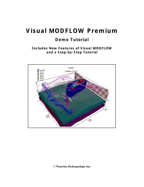
<strong>Visual</strong> <strong>MODFLOW</strong> <strong>Premium</strong><br />
<strong>Demo</strong> <strong>Tutorial</strong><br />
Includes New Features of <strong>Visual</strong> <strong>MODFLOW</strong><br />
and a Step-by-Step <strong>Tutorial</strong><br />
© Waterloo Hydrogeologic Inc.
© Waterloo Hydrogeologic Inc.<br />
Table of Contents<br />
Introduction to <strong>Visual</strong> <strong>MODFLOW</strong> . . . . . . . . . . . . . . . . . . . . . . . . . . . . . . . . 1<br />
What’s New in <strong>Visual</strong> <strong>MODFLOW</strong> . . . . . . . . . . . . . . . . . . . . . . . . . . . . . . . . . . . . . . .1<br />
New Features in <strong>Visual</strong> <strong>MODFLOW</strong> v.4.1 . . . . . . . . . . . . . . . . . . . . . . . . . . . . . . . . . . . . . . . . . . . . 1<br />
New Features in <strong>Visual</strong> <strong>MODFLOW</strong> v.4.0 . . . . . . . . . . . . . . . . . . . . . . . . . . . . . . . . . . . . . . . . . . . . 2<br />
Starting <strong>Visual</strong> <strong>MODFLOW</strong> . . . . . . . . . . . . . . . . . . . . . . . . . . . . . . . . . . . . . . . . . . . . . . . . . . . . . . . 2<br />
About the Interface . . . . . . . . . . . . . . . . . . . . . . . . . . . . . . . . . . . . . . . . . . . . . . . . . . . . . . .2<br />
Getting Around In <strong>Visual</strong> <strong>MODFLOW</strong> . . . . . . . . . . . . . . . . . . . . . . . . . . . . . . . . . . . . . . . . . . . . . . 3<br />
Screen Layout . . . . . . . . . . . . . . . . . . . . . . . . . . . . . . . . . . . . . . . . . . . . . . . . . . . . . . . . . . . . . . . . . . 4<br />
Contacting WHI . . . . . . . . . . . . . . . . . . . . . . . . . . . . . . . . . . . . . . . . . . . . . . . . . . . . . . .5<br />
<strong>Visual</strong> <strong>MODFLOW</strong> <strong>Premium</strong> <strong>Tutorial</strong> . . . . . . . . . . . . . . . . . . . . . . . . . . . . . . 7<br />
Introduction . . . . . . . . . . . . . . . . . . . . . . . . . . . . . . . . . . . . . . . . . . . . . . . . . . . . . . . . . . . . .7<br />
Description of the Example Model . . . . . . . . . . . . . . . . . . . . . . . . . . . . . . . . . . . . . . . .7<br />
How to Use this <strong>Tutorial</strong> . . . . . . . . . . . . . . . . . . . . . . . . . . . . . . . . . . . . . . . . . . . . . . . .9<br />
Terms and Notations . . . . . . . . . . . . . . . . . . . . . . . . . . . . . . . . . . . . . . . . . . . . . . . . . . . . . . . . . . . . . 9<br />
Module I: Creating and Defining a Flow Model . . . . . . . . . . . . . . . . . . . . . . 9<br />
Section 1: Generating a New Model . . . . . . . . . . . . . . . . . . . . . . . . . . . . . . . . . . . . . . . . . .9<br />
Step 1 . . . . . . . . . . . . . . . . . . . . . . . . . . . . . . . . . . . . . . . . . . . . . . . . . . . . . . . . . . . . . .10<br />
Step 2 . . . . . . . . . . . . . . . . . . . . . . . . . . . . . . . . . . . . . . . . . . . . . . . . . . . . . . . . . . . . . .12<br />
Step 3 . . . . . . . . . . . . . . . . . . . . . . . . . . . . . . . . . . . . . . . . . . . . . . . . . . . . . . . . . . . . . .12<br />
Step 4 . . . . . . . . . . . . . . . . . . . . . . . . . . . . . . . . . . . . . . . . . . . . . . . . . . . . . . . . . . . . . .14<br />
Add Air Photo . . . . . . . . . . . . . . . . . . . . . . . . . . . . . . . . . . . . . . . . . . . . . . . . . . . . . . . . . . . . . . . . . 17<br />
Section 2: Refining the Model Grid . . . . . . . . . . . . . . . . . . . . . . . . . . . . . . . . . . . . . . . . . .20<br />
Section 3: Adding Pumping Wells . . . . . . . . . . . . . . . . . . . . . . . . . . . . . . . . . . . . . . . . . . .29<br />
Section 4: Assigning Flow Properties . . . . . . . . . . . . . . . . . . . . . . . . . . . . . . . . . . . . . . . .30<br />
Section 5: Assigning Flow Boundary Conditions . . . . . . . . . . . . . . . . . . . . . . . . . . . . . . .36<br />
Assigning Aquifer Recharge to the Model . . . . . . . . . . . . . . . . . . . . . . . . . . . . . . . . . . . . . . . . . . . 36<br />
Assigning Constant Head Boundary Conditions . . . . . . . . . . . . . . . . . . . . . . . . . . . . . . . . . . . . . . . 37<br />
Assigning River Boundary Conditions . . . . . . . . . . . . . . . . . . . . . . . . . . . . . . . . . . . . . . . . . . . . . . 40<br />
Section 6: Particle Tracking . . . . . . . . . . . . . . . . . . . . . . . . . . . . . . . . . . . . . . . . . . . . . . . .42<br />
Module II: The Contaminant Transport Model . . . . . . . . . . . . . . . . . . . . . . 43<br />
Section 7: Setting Up the Transport Model . . . . . . . . . . . . . . . . . . . . . . . . . . . . . . . . . . . .43<br />
Contaminant Transport Properties . . . . . . . . . . . . . . . . . . . . . . . . . . . . . . . . . . . . . . . .43<br />
Viewing Sorption Properties . . . . . . . . . . . . . . . . . . . . . . . . . . . . . . . . . . . . . . . . . . . . . . . . . . . . . . 43<br />
Assigning Dispersion Coefficients . . . . . . . . . . . . . . . . . . . . . . . . . . . . . . . . . . . . . . . . . . . . . . . . . 44<br />
Section 8: Transport Boundary Conditions . . . . . . . . . . . . . . . . . . . . . . . . . . . . . . . . . . . .45<br />
Section 9: Adding Observation Wells . . . . . . . . . . . . . . . . . . . . . . . . . . . . . . . . . . . . . . . .45<br />
Module III: Running <strong>Visual</strong> <strong>MODFLOW</strong> . . . . . . . . . . . . . . . . . . . . . . . . . . 47<br />
Section 10: <strong>MODFLOW</strong> Run Options . . . . . . . . . . . . . . . . . . . . . . . . . . . . . . . . . . . . . . .47<br />
<strong>MODFLOW</strong> Solver Options . . . . . . . . . . . . . . . . . . . . . . . . . . . . . . . . . . . . . . . . . . . . . . . . . . . . . . 48<br />
Dry Cell Wetting Options . . . . . . . . . . . . . . . . . . . . . . . . . . . . . . . . . . . . . . . . . . . . . . . . . . . . . . . . 48<br />
Section 11: MT3DMS Run Options . . . . . . . . . . . . . . . . . . . . . . . . . . . . . . . . . . . . . . . . .49<br />
MT3DMS Solver Settings . . . . . . . . . . . . . . . . . . . . . . . . . . . . . . . . . . . . . . . . . . . . . . . . . . . . . . . . 49
MT3DMS Output Times . . . . . . . . . . . . . . . . . . . . . . . . . . . . . . . . . . . . . . . . . . . . . . . . . . . . . . . . . 50<br />
Section 12: Running the Simulation . . . . . . . . . . . . . . . . . . . . . . . . . . . . . . . . . . . . . . . . .51<br />
MODULE IV: Output <strong>Visual</strong>ization . . . . . . . . . . . . . . . . . . . . . . . . . . . . . . . 51<br />
Section 13: Head Contours . . . . . . . . . . . . . . . . . . . . . . . . . . . . . . . . . . . . . . . . . . . . . . . .52<br />
Displaying a Color Map of Heads . . . . . . . . . . . . . . . . . . . . . . . . . . . . . . . . . . . . . . . . . . . . . . . . . . 54<br />
Section 14: Velocity Vectors . . . . . . . . . . . . . . . . . . . . . . . . . . . . . . . . . . . . . . . . . . . . . . .56<br />
Section 15: Pathlines . . . . . . . . . . . . . . . . . . . . . . . . . . . . . . . . . . . . . . . . . . . . . . . . . . . . .57<br />
Section 16: Concentration Contours . . . . . . . . . . . . . . . . . . . . . . . . . . . . . . . . . . . . . . . . .59<br />
Section 17: Concentration vs. Time Graphs . . . . . . . . . . . . . . . . . . . . . . . . . . . . . . . . . . .64<br />
Module V: <strong>Visual</strong> <strong>MODFLOW</strong> 3D-Explorer . . . . . . . . . . . . . . . . . . . . . . . . 66<br />
Section 18: Starting <strong>Visual</strong> <strong>MODFLOW</strong> 3D-Explorer . . . . . . . . . . . . . . . . . . . . . . . . . . .66<br />
Section 19: Changing the Default Settings . . . . . . . . . . . . . . . . . . . . . . . . . . . . . . . . . . . .67<br />
Section 20: Using the Navigation Tools . . . . . . . . . . . . . . . . . . . . . . . . . . . . . . . . . . . . . .67<br />
Section 21: Creating a 3D Contaminant Plume . . . . . . . . . . . . . . . . . . . . . . . . . . . . . . . . .68<br />
Customizing the Color Legend . . . . . . . . . . . . . . . . . . . . . . . . . . . . . . . . . . . . . . . . . . . . . . . . . . . . 70<br />
Selecting Output Times . . . . . . . . . . . . . . . . . . . . . . . . . . . . . . . . . . . . . . . . . . . . . . . . . . . . . . . . . . 71<br />
Section 22: <strong>Visual</strong>izing Model Input Data . . . . . . . . . . . . . . . . . . . . . . . . . . . . . . . . . . . .71<br />
Section 23: Defining Surfaces (Cross-Sections and Slices) . . . . . . . . . . . . . . . . . . . . . . .72<br />
Section 24: Creating a Cut-Away View . . . . . . . . . . . . . . . . . . . . . . . . . . . . . . . . . . . . . .74<br />
Section 25: Creating a Color Map of Head Values . . . . . . . . . . . . . . . . . . . . . . . . . . . . . .76<br />
Customizing the Color Legend . . . . . . . . . . . . . . . . . . . . . . . . . . . . . . . . . . . . . . . . . . . . . . . . . . . . 77<br />
Section 26: Printing to a Graphics File . . . . . . . . . . . . . . . . . . . . . . . . . . . . . . . . . . . . . . .78<br />
<strong>Visual</strong> <strong>MODFLOW</strong> Order Form . . . . . . . . . . . . . . . . . . . . . . . . . . . . . . . . . . . . . . . . . . . .80
1<br />
Introduction to <strong>Visual</strong> <strong>MODFLOW</strong><br />
<strong>Visual</strong> <strong>MODFLOW</strong> is the most complete and easy-to-use modeling environment for<br />
practical applications in three-dimensional groundwater flow and contaminant transport<br />
simulations. This fully-integrated package combines <strong>MODFLOW</strong>, <strong>MODFLOW</strong>-<br />
SURFACT, MODPATH, ZoneBudget, MT3Dxx/RT3D, MGO, and WinPEST with the<br />
most intuitive and powerful graphical interface available. The logical menu structure and<br />
easy-to-use graphical tools allow you to:<br />
• easily dimension the model domain and select units<br />
• conveniently assign model properties and boundary conditions<br />
• run the model simulations<br />
• calibrate the model using manual or automated techniques<br />
• optimize the pumping well rates and locations<br />
• visualize the results using 2D or 3D graphics<br />
The model input parameters and results can be visualized in 2D (cross-section and plan<br />
view) or 3D at any time during the development of the model, or the displaying of the<br />
results. For complete three-dimensional groundwater flow and contaminant transport<br />
modeling, <strong>Visual</strong> <strong>MODFLOW</strong> is the only software package you will need.<br />
When you purchase <strong>Visual</strong> <strong>MODFLOW</strong>, or any Waterloo Hydrogeologic software<br />
product, you not only get the best software in the industry, you also gain the reputation of<br />
the company behind the product, and professional technical support for the software from<br />
our team of qualified groundwater modeling professionals. Waterloo Hydrogeologic has<br />
been developing groundwater software since 1989, and our software is recognized,<br />
accepted and used by more than 10,000 groundwater professionals in over 90 countries<br />
around the world. This type of recognition is invaluable in establishing the credibility of<br />
your modeling software to clients and regulatory agencies. <strong>Visual</strong> <strong>MODFLOW</strong> is<br />
continuously being upgraded with new features to fulfill our clients needs.<br />
What’s New in <strong>Visual</strong> <strong>MODFLOW</strong><br />
The main interface for <strong>Visual</strong> <strong>MODFLOW</strong> has much of the same user-friendly look and<br />
feel as the previous versions of <strong>Visual</strong> <strong>MODFLOW</strong>, but what’s “under the hood” has been<br />
dramatically improved to give you more powerful tools for entering, modifying,<br />
analyzing, and presenting your groundwater modeling data. Some of the more significant<br />
upgrade features in the latest version of <strong>Visual</strong> <strong>MODFLOW</strong> are described below.<br />
New Features in <strong>Visual</strong> <strong>MODFLOW</strong> v.4.2<br />
MIKE 11 Integration<br />
DHI's MIKE 11 software package is a versatile and modular engineering tool for modeling<br />
conditions in rivers, lakes/reservoirs, irrigation canals and other inland water systems.<br />
1
MIKE 11 is now integrated into <strong>Visual</strong> <strong>MODFLOW</strong> with the use of OpenMI technology,<br />
providing the tools for integrated surface water - groundwater flow.<br />
PHT3D Integration<br />
PHT3D is a multi-component transport model for three-dimensional reactive transport in<br />
saturated porous media.<br />
MT3DMS 5.1 Integration<br />
Support for MT3DMS v.5.1, which includes an option to simulate zeroth-order decay or<br />
production as documented in Zheng (2005). Zeroth-order reactions may be useful for<br />
describing certain types of biogeochemical decay or production. In addition, zeroth-order<br />
reactions can be used for direct simulation of groundwater ages or calculation of<br />
parameter sensitivities.<br />
New Features in <strong>Visual</strong> <strong>MODFLOW</strong> v.4.1<br />
About the Interface<br />
• Integrated the USGS SEAWAT 2000 engine to solve variable density flow such<br />
as seawater intrusion modeling problems<br />
• Integrated the latest release of USGS <strong>MODFLOW</strong> 2000 (version 1.15.00, August<br />
6, 2004)<br />
• Integrated the MT3DMS version 4.5<br />
• Implemented VCONT calculation options that allow you to chose between<br />
VCONT values calculated from the Ground Surface (top of layer 1) or Initial<br />
Heads<br />
• Improved project creation wizard help you to choose the right numeral engines to<br />
meet your objectives<br />
• Support the new Geometric Multigrid Solver (GMG) solver from USGS<br />
• Support the latest Algebraic Multigrid Methods for Systems (SAMG) solver<br />
optimized for <strong>MODFLOW</strong><br />
The <strong>Visual</strong> <strong>MODFLOW</strong> interface has been specifically designed to increase modeling<br />
productivity, and decrease the complexities typically associated with building threedimensional<br />
groundwater flow and contaminant transport models. In order to simplify the<br />
graphical interface, <strong>Visual</strong> <strong>MODFLOW</strong> is divided into three separate modules:<br />
• The Input section<br />
• The Run section<br />
• The Output section.<br />
Each of these modules is accessed from the Main Menu when a <strong>Visual</strong> <strong>MODFLOW</strong><br />
project is started, or an existing project is opened. The Main Menu serves as a link to<br />
seamlessly switch between each of these modules, to define or modify the model input<br />
parameters, run the simulations, calibrate and optimize the model, and display results.<br />
The Input section allows the user to graphically assign all of the necessary input<br />
parameters for building a three-dimensional groundwater flow and contaminant transport<br />
model. The input menus represent the basic "model building blocks" for assembling a data<br />
set using <strong>MODFLOW</strong>, <strong>MODFLOW</strong>-SURFACT, MODPATH, ZoneBudget, and MT3D/<br />
About the Interface 2
RT3D. These menus are displayed in a logical order to guide the modeler through the steps<br />
necessary to design a groundwater flow and contaminant transport model.<br />
The Run section allows the user to modify the various <strong>MODFLOW</strong>, <strong>MODFLOW</strong>-<br />
SURFACT, MODPATH, MT3D/RT3D, MGO, and WinPEST parameters and options<br />
which are run-specific. These include selecting initial head estimates, setting solver<br />
parameters, activating the re-wetting package, specifying the output controls, etc. Each of<br />
these menu selections has default settings, which are capable of running most simulations.<br />
The Output section allows the user to display all of the modeling and calibration results<br />
for <strong>MODFLOW</strong>, <strong>MODFLOW</strong>-SURFACT, MODPATH, ZoneBudget, and MT3D/RT3D.<br />
The output menus allow you to select, customize, overlay the various display options, and<br />
export images for presenting the modeling results.<br />
Starting <strong>Visual</strong> <strong>MODFLOW</strong><br />
Once <strong>Visual</strong> <strong>MODFLOW</strong> has been installed on your computer, simply double-click on the<br />
<strong>Visual</strong> <strong>MODFLOW</strong> shortcut icon, or click on Start/Programs/WHI Software/<strong>Visual</strong><br />
<strong>MODFLOW</strong> /<strong>Visual</strong> <strong>MODFLOW</strong>.<br />
Getting Around In <strong>Visual</strong> <strong>MODFLOW</strong><br />
The Main Menu screen contains the following options:<br />
File Select a file utility, or exit <strong>Visual</strong> <strong>MODFLOW</strong>.<br />
Input Design, modify, and visualize the model grid and input parameters.<br />
Run Enter or modify the model run settings and run the numerical simulations, in<br />
either project mode or batch mode.<br />
Output <strong>Visual</strong>ize the model output (simulation results) using contour maps, color<br />
maps, velocity vectors, pathlines, time-series graphs, scatter plots, etc.<br />
Setup Select the “numeric engine” for both the flow and transport simulation(s).<br />
Help Get general information on how to use <strong>Visual</strong> <strong>MODFLOW</strong>.<br />
A Microsoft compatible mouse performs as follows:<br />
Left button: This is the regular ‘click’ button. By holding it down on top of an input<br />
box and dragging the mouse, it will also highlight the characters that will<br />
be overwritten by the next typed character.<br />
Right button: This button has different functions depending on the context. For<br />
example, it closes polygons or ends a line during the assignment of<br />
properties, boundaries, etc. During grid design, it also locates grid rows or<br />
columns on precise co-ordinates. Using the right button brings up a submenu<br />
to copy, paste, delete, etc.<br />
3
Screen Layout<br />
The shortcut keys can be used to access toolbar items and to select many buttons<br />
and can be used anytime an item or button text has an underlined letter. Simply press the<br />
key and the letter key at the same time to access the item or select the button. The<br />
number and letter keys are active only when numerical or text input is required; all other<br />
keys are ignored by <strong>Visual</strong> <strong>MODFLOW</strong>.<br />
After opening a <strong>Visual</strong> <strong>MODFLOW</strong> project and selecting the Input module, a screen<br />
layout similar to the figure below will appear.<br />
Top Menu Bar<br />
Side Menu Bar<br />
Navigation Cube<br />
Co-ordinates area<br />
Status Bar<br />
Function Buttons<br />
Project Name<br />
Top Menu Bar: Contains specific data category menus for each<br />
section of the interface (Input, Run and<br />
Output).<br />
Side Menu Bar: Contains the View Control buttons plus tool<br />
buttons specific for each data category. The<br />
view options are as follows:<br />
[View Column] View a cross-section along a column.<br />
[View Row] View a cross-section along a row.<br />
[View Layer] Switch from cross-section to plan view.<br />
[Goto] View a specified column, row, or layer.<br />
[Previous] View previous column, row, or layer.<br />
Transport Variant<br />
[Next] View next column, row, or layer.<br />
Navigator Cube: Provides a simplified 3D representation of the model domain<br />
highlighting the current layer, column, and row being viewed.<br />
Co-ordinates Area: Shows the current location of the mouse pointer in model coordinates<br />
(X, Y, Z) and cell indices (I, J, K).<br />
About the Interface 4
Contacting WHI<br />
Status Bar: Describes the functionality and use of the feature currently<br />
highlighted by the cursor.<br />
Function Buttons:<br />
[F1-Help] Opens the general help window<br />
[F2-3D] Opens the <strong>Visual</strong> <strong>MODFLOW</strong> 3D-Explorer<br />
[F3-Save] Saves the current data for the model.<br />
[F4-Map] Import and display .DXF, .SHP, or .graphics image files (.BMP,<br />
.JPG, .TIF, .GIF, .PNG)<br />
[F5–Zoom in] Enlarge the display of a selected rectangular area<br />
[F6–Zoom out] Resets the display area to show the entire model domain<br />
[F7-Pan] Drag the current view of the model in any direction to display a<br />
different model region<br />
[F8–Vert exag] Set the vertical exaggeration value for viewing cross sections<br />
along a row or column<br />
[F9-Overlay] Opens the Overlay Control window to make selected<br />
overlays visible and to customize the priority (order) in which they appear<br />
[F10–Main Menu] Returns to the Main Menu screen.<br />
The purpose of this tutorial is to demonstrate the ease of building, calibrating, and running<br />
a three-dimensional groundwater flow and contaminant transport model. Unfortunately,<br />
this tutorial can only cover a few of the many analytical capabilities and graphical features<br />
that make <strong>Visual</strong> <strong>MODFLOW</strong> the leading software package for groundwater flow and<br />
contaminant transport modeling.<br />
If this tutorial has not covered some aspects of the software that you are interested in, we<br />
encourage you to continue to consult the on-line help files and the carefully read the<br />
<strong>Visual</strong> <strong>MODFLOW</strong> User’s Manual. If you would like to speak with a technical<br />
representative about how <strong>Visual</strong> <strong>MODFLOW</strong> could be applied to solve your particular<br />
needs, please contact at:<br />
Waterloo Hydrogeologic Inc.<br />
460 Phillip Street, Suite 101<br />
Waterloo, Ontario, N2L 5J2<br />
5
Tel: (519) 746-1798<br />
Fax: (519) 885-5262<br />
E-mail: techsupport@flowpath.com<br />
Web: www.waterloohydrogeologic.com<br />
About the Interface 6
2<br />
<strong>Visual</strong> <strong>MODFLOW</strong> <strong>Premium</strong> <strong>Tutorial</strong><br />
Introduction<br />
This chapter contains a step-by-step tutorial to guide you through the process of using<br />
Waterloo Hydrogeologic’s <strong>Visual</strong> <strong>MODFLOW</strong> <strong>Premium</strong> <strong>Demo</strong> version. This tutorial will<br />
guide you through the steps required to:<br />
• Design the model grid and assign properties and boundary conditions,<br />
• Configure <strong>Visual</strong> <strong>MODFLOW</strong> to run the groundwater flow, particle tracking, and<br />
mass transport simulations, and<br />
• <strong>Visual</strong>ize the results using two- and three-dimensional graphics<br />
For your convenience, the <strong>Visual</strong> <strong>MODFLOW</strong> <strong>Demo</strong> version allows you to install a complete<br />
set of input data files and simulation results for the example model that you will build. The<br />
instructions for the tutorial are provided in a step-wise format that allows you to choose the<br />
features that you are interested in examining without having to complete the entire exercise.<br />
Limitations of the <strong>Demo</strong> version<br />
How to Use this <strong>Tutorial</strong><br />
The <strong>Demo</strong> version of <strong>Visual</strong> <strong>MODFLOW</strong> is fully functional, and you may create, open,<br />
modify, translate, and run any model, as long as the model meets the following restrictions:<br />
• The grid is no finer than 40 Rows X 40 Columns X 3 Layers<br />
• There are no more than 3 property zones<br />
• There are no more than 2 pumping wells<br />
NOTE: If you have purchased a license and are using this tutorial to familiarize yourself with<br />
the program, keep in mind that some features are only available in a Pro or <strong>Premium</strong> version.<br />
This tutorial is divided into five modules, and each module contains a number of sections.<br />
The tutorial is designed so that the user can begin at any of the modules in order to examine<br />
specific aspects of the <strong>Visual</strong> <strong>MODFLOW</strong> environment. Each section is written in an easy-touse<br />
step-wise format. The modules are arranged as follows.<br />
Module I - Creating and Defining a Flow Model<br />
Module II - The Contaminant Transport Model<br />
Module III - Running <strong>Visual</strong> <strong>MODFLOW</strong><br />
Module IV - Output <strong>Visual</strong>ization<br />
Module V - <strong>Visual</strong> <strong>MODFLOW</strong> 3D Explorer<br />
<strong>Visual</strong> <strong>MODFLOW</strong>: Introduction and <strong>Tutorial</strong> 7
Terms and Notations<br />
For the purposes of this tutorial, the following terms and notations will be used:<br />
Type:- type in the given word or value<br />
Select:- click the left mouse button where indicated<br />
- press the key<br />
↵ - press the key<br />
- Click the left mouse button where indicated<br />
- double-click the left mouse button where indicated<br />
Description of the Example Model<br />
[...] - denotes a button to click on, either in a window, or in the side or bottom menu<br />
bars.<br />
The bold faced type indicates menu or window items to click on or values to type in.<br />
Some of the more significant upgrade features included in the latest versions of<br />
<strong>Visual</strong> <strong>MODFLOW</strong> are described in italic form.<br />
The site is located near an airport just outside of Waterloo. The surficial geology at the site<br />
consists of an upper sand and gravel aquifer, a lower sand and gravel aquifer, and a clay and<br />
silt aquitard separating the upper and lower aquifers. The relevant site features consist of a<br />
plane refuelling area, a municipal water supply well field, and a discontinuous aquitard zone.<br />
These features are illustrated in the following figure:<br />
The municipal well field consists of two wells. The east well pumps at a constant rate of 550<br />
m 3 /day, while the west well pumps at a constant rate of 400 m 3 /day. Over the past ten years,<br />
airplane fuel has periodically been spilled in the refuelling area and natural infiltration has<br />
produced a plume of contamination in the upper aquifer. This tutorial will guide you through<br />
the steps necessary to build a groundwater flow and contaminant transport model for this site.<br />
Introduction 8
This model will demonstrate the potential impact of the fuel contamination on the municipal<br />
water supply wells.<br />
When discussing the site, in plan view, the top of the site will be designated as north, the<br />
bottom of the site as south, and the left side and right side as west and east, respectively.<br />
Groundwater flow is from north to south (top to bottom) in a three-layer system consisting of<br />
an upper unconfined aquifer, an intervening middle aquitard, and a lower confined aquifer, as<br />
illustrated in the following figure. The upper aquifer and lower aquifers have a hydraulic<br />
conductivity of 2e -4 m/sec, and the aquitard has a hydraulic conductivity of 1e -10 m/sec.<br />
Module I: Creating and Defining a Flow Model<br />
The project creation wizard was re-designed for version 4.1. Most of the default options and<br />
parameter values for flow, transport, grid, and project are now set during the initial set-up to<br />
avoid having to enter them later in various parts of the program.<br />
Section 1: Generating a New Model<br />
The first module will take you through the steps necessary to generate a new model data set<br />
using the <strong>Visual</strong> <strong>MODFLOW</strong> modeling environment.<br />
On your Windows desktop, you will see an icon for <strong>Visual</strong> <strong>MODFLOW</strong>:<br />
to start the <strong>Visual</strong> <strong>MODFLOW</strong> program<br />
To create your new model:<br />
File from the top menu bar<br />
New<br />
A Create new model window will appear.<br />
For your convenience, we have already created a model following this step-by-step tutorial.<br />
The model is located in the default directory C:\VMODNT\<strong>Tutorial</strong>.<br />
It is recommended that you create a new folder, and save the new model in this folder.<br />
To create a new folder:<br />
<br />
<strong>Visual</strong> <strong>MODFLOW</strong>: Introduction and <strong>Tutorial</strong> 9
Step 1: Project Settings<br />
Type in a new folder name.<br />
on the new folder<br />
Type: Airport in the File name field<br />
[Save]<br />
NOTE: If you choose the default directory (C:\VMODNT\<strong>Tutorial</strong>) and type in the same<br />
Airport file name, a warning message may appear if the Airport.vmf file has already been<br />
created.<br />
[No] to save your new model in a different folder, or<br />
[Yes] to overwrite the existing model.<br />
<strong>Visual</strong> <strong>MODFLOW</strong> automatically adds a .VMF extension onto the end of the filename.<br />
Next, the Model Setup is described in four consecutive steps.<br />
In Step 1, the following window is used to select:<br />
• the desired Project Information<br />
• Units associated with various flow and transport parameters, and<br />
• the desired Engines for the Flow and Transport simulation<br />
For the Flow model, the following Numeric Engines are available:<br />
• USGS <strong>MODFLOW</strong>-96 from WHI (saturated, constant density)<br />
• USGS <strong>MODFLOW</strong>-2000 from WHI (saturated, constant density)<br />
• USGS SEAWAT 2000 (saturated, variable density)<br />
• <strong>MODFLOW</strong>-SURFACT from HGL (variably saturated)<br />
In this example, <strong>MODFLOW</strong>-2000 is selected.<br />
Section 1: Generating a New Model 10
Step 2: Flow Settings<br />
<strong>Visual</strong> <strong>MODFLOW</strong> supports all of the latest versions of the public domain and proprietary<br />
programs for contaminant transport modeling, including:<br />
• MT3DMS<br />
• MT3Dv150<br />
• MT3D99<br />
• RT3Dv1.0<br />
• RT3Dv2.5<br />
• PHT3Dv.1.45<br />
<strong>Visual</strong> <strong>MODFLOW</strong> now supports PHT3D v.1.45, a multi-component transport model for<br />
three-dimensional reactive transport in saturated porous media. For a sample application of<br />
PHT3D, please refer to the PHT3D <strong>Tutorial</strong>; for more details, please consult your Users<br />
Manual.<br />
In addition, <strong>Visual</strong> <strong>MODFLOW</strong> now supports MT3DMS v.5.1, including support for zerothorder<br />
reactions.<br />
Note: The MT3DMS, MT3D99 and RT3D, PHT3D transport engines allow for multi-species<br />
contaminant transport. MT3D150 allows only a single species to be modeled.<br />
[Yes] radio button, to enable the Transport Simulation options<br />
In this example, MT3DMS is selected by default, and will be used for the simulation.<br />
Under the Units section, select the following information for each model input data type.<br />
Length: meters<br />
Time: day<br />
Conductivity: m/sec<br />
Pumping Rate: m^3/day<br />
Recharge: mm/year<br />
Mass: kilogram<br />
Concentration: milligrams/liter<br />
[Next] to accept these values<br />
In Step 2, the following window will appear displaying the default parameter values for the<br />
Flow simulation.<br />
<strong>Visual</strong> <strong>MODFLOW</strong>: Introduction and <strong>Tutorial</strong> 11
Step 3: Transport Settings<br />
type: 7300 for the Steady State Simulation time<br />
The Start Date and Start Time of the model are corresponding to the beginning of the<br />
simulation time period. Currently, this date is relevant only for transient flow simulations<br />
where recorded field data may be imported for defining time schedules for selected boundary<br />
conditions (Constant Head, River, General Head and Drain).<br />
[Next] to accept these values<br />
In Step 3, the following window will appear displaying the default parameter values for the<br />
Transport simulation.<br />
Section 1: Generating a New Model 12
In order to support all of the available options for the multi-species reactive transport<br />
programs, <strong>Visual</strong> <strong>MODFLOW</strong> requires you to setup the initial conditions for the contaminant<br />
transport scenario (e.g. number of chemical species, names of each chemical species, initial<br />
concentrations, decay rates, partitioning coefficients, etc.). Each scenario is referred to as a<br />
Transport Variant, and you can have more than one variant for a given flow model.<br />
By default <strong>Visual</strong> <strong>MODFLOW</strong> creates a variant named VAR001.<br />
We will now edit this variant to setup the model for transport processes.<br />
The default transport variant will use MT3DMS as the numeric engine, with no sorption or<br />
reaction terms.<br />
For this tutorial you will add a linear sorption process to the transport variant.<br />
in the Sorption combo box<br />
Select Linear Isotherm [equilibrium-controlled]<br />
For this tutorial you will not be simulating any decay or degradation of the contaminant, so<br />
the default Reactions settings of No kinetic reactions will be fine.<br />
Below the Sorption and Reaction settings are three tabs labelled:<br />
• Species<br />
• Model Params<br />
• Species Params<br />
In the Species tab you will see a spreadsheet view with labelled column headings. The last<br />
two columns are labelled with MT3D variable names.<br />
The chemical species being simulated in this model is JP-4. <strong>Visual</strong> <strong>MODFLOW</strong> allows you<br />
to use the real names of the simulated chemicals in order to easily identify them in contour<br />
maps and graphs.<br />
Type the following information for the chemical species:<br />
Type: JP-4 in the Designation column<br />
<strong>Visual</strong> <strong>MODFLOW</strong>: Introduction and <strong>Tutorial</strong> 13
Step 4: Model Domain<br />
Type: Spilled Jet Fuel in the Component Description column<br />
in the Mobile column and select Yes<br />
Type: 0 in the SCONC [mg/L] column<br />
Type: 1e-7 in SP1 [1/(mg/L)] column<br />
The species information is now set up properly, and should appear similar to the figure shown<br />
below.<br />
This completes the setup for the Transport Engine. You are now ready to exit the Transport<br />
Engine Options window.<br />
[Next] to continue.<br />
Step 4 is Creating the Model Grid (see figure below).<br />
Section 1: Generating a New Model 14
In this step you can Import a site map, specify the dimensions of the Model Domain, and<br />
define the number of rows, columns, and layers for the finite difference grid.<br />
Enter the following number of rows, columns, and layers to be used in the model. Type the<br />
following into the Model Domain section,<br />
Columns (j): 30<br />
Rows (i): 30<br />
Layers (k): 3<br />
Zmin: 0<br />
Zmax: 18<br />
Import a site map<br />
Next, you must specify the location and the file name of the .DXF background map.<br />
[Browse]<br />
Navigate to the vmodnt\<strong>Tutorial</strong>\Airport directory and select the following file:<br />
Sitemap.dxf<br />
[Open]<br />
[Finish] to accept these settings<br />
<strong>Visual</strong> <strong>MODFLOW</strong> provides support for importing and displaying multiple site maps using<br />
the most common graphics image formats, including .JPG, .GIF, .TIF, .PNG, and .BMP files.<br />
Additionally, a transparency setting may be applied to the imported images in order to<br />
display multiple images simultaneously, or to view other model attributes underneath the site<br />
map image overlay.<br />
A Select Model Region window will appear prompting you to define the extents of the<br />
model area. <strong>Visual</strong> <strong>MODFLOW</strong> will read the minimum and maximum co-ordinates from the<br />
site map (Sitemap.dxf) and suggest a default location that is centred in the model domain.<br />
<strong>Visual</strong> <strong>MODFLOW</strong>: Introduction and <strong>Tutorial</strong> 15
Type the following values over the numbers shown on the screen:<br />
Display area: X1: 0 <br />
Y1: 0 <br />
X2: 2000 <br />
Y2: 2000 <br />
Model Origin: X: 0 <br />
Y: 0 <br />
Angle: 0 <br />
Model Corners: X1: 0 <br />
Y1: 0 <br />
X2: 2000 <br />
Y2: 2000 ↵<br />
[OK] to accept the model dimensions.<br />
A File attributes window will appear to indicate that the “Sitemap.dxf” is being saved inside<br />
the <strong>Visual</strong> <strong>MODFLOW</strong> project with the name “Airport.Sitemap.MAP”.<br />
[OK]<br />
The Input menu will open, and a uniformly spaced 30 x 30 x 3 finite-difference grid will<br />
automatically be generated within the model domain. The Grid and site map will appear on<br />
the screen, as shown in the following figure:<br />
Section 1: Generating a New Model 16
Add Air Photo<br />
By default the Grid screen is loaded when you first enter the Input module.<br />
At this time, you may add an additional map for improved visualization; you will add an<br />
airphoto of the site, in bitmap format.<br />
F4 (Map) button from the bottom toolbar.<br />
A dialog will appear where you can specify the file to import. Browse to<br />
vmodnt\<strong>Tutorial</strong>\Airport.<br />
At the bottom of the dialog, under Files of Type,<br />
Graphics File from the list.<br />
Airport.Airphoto.bmp file from the list.<br />
[Open]<br />
<strong>Visual</strong> <strong>MODFLOW</strong>: Introduction and <strong>Tutorial</strong> 17
A “Select Model Region” dialog will then appear, as shown below.<br />
In order to map the pixels of the image to a coordinate system, the image must have two<br />
georeference points with known coordinates. These georeference points can be defined using<br />
the procedure described below. For this image, the two points have been marked with a red X,<br />
and are located at opposite ends of the airport’s main runway (and are circled in the image<br />
above).<br />
To set the georeference points,<br />
• Click on the red X located on the left side of the map. A Georeference point<br />
dialog will appear prompting for the X1 and Y1 world coordinates of the selected<br />
location:<br />
• Enter the X1 and Y1 coordinates for this point.<br />
for X1, type: 502<br />
for Y1, type: 1212<br />
• Click [OK]<br />
• Click on the red X located on the right side of the map. A Georeference point<br />
dialog will appear prompting for the X2 and Y2 world coordinates of the selected<br />
Section 1: Generating a New Model 18
location:<br />
for X2, type: 1619<br />
for Y2, type: 1863<br />
• Click [OK]<br />
A box will appear around the map region.<br />
• Click [OK] to continue<br />
A confirmation message will appear, displaying the filename of the georeferenced image.<br />
• Click [OK] to continue<br />
If the map image was correctly georeferenced, the river and runway locations should match<br />
up closely with those digitized in the AutoCAD Sitemap.dxf file. The display should now be<br />
similar to the one shown below.<br />
The site map properties can be defined in the overlay control.<br />
F9 (Overlay Control) button from the bottom toolbar.<br />
<strong>Visual</strong> <strong>MODFLOW</strong>: Introduction and <strong>Tutorial</strong> 19
For the remainder of this tutorial, the screenshots will not display the airphoto; you may keep<br />
this visible if you wish.<br />
Map-Airport.Airphoto [Bitmap] checkbox, to turn off this map.<br />
[OK]<br />
This concludes Section 1: Generating a new Model. In the next section, you will refine the<br />
model grid.<br />
Section 2: Refining the Model Grid<br />
The Grid screen provides a complete assortment of graphical tools for refining the model<br />
grid, delineating inactive grid zones, importing layer surface elevations, assigning elevations,<br />
optimizing (smoothing) the grid spacing, and contouring the layer surface elevations.<br />
This section describes the steps necessary to refine the model grid in areas of interest, such as<br />
around the water supply wells, refueling area, and area of discontinuous aquitard. The reason<br />
for refining the grid is to get more detailed simulation results in areas of interest, or in zones<br />
where you anticipate steep hydraulic gradients. For example, if drawdown is occurring<br />
around the well, the water table will have a smoother surface if you use a finer grid spacing.<br />
Also, layer properties can be assigned more correctly on a finer grid.<br />
To refine the grid in the X-direction,<br />
[Edit Grid >] Edit Columns<br />
A Columns window will appear showing the options you have for editing the grid columns.<br />
By default the Add option is selected, and new grid lines can be added by clicking the mouse<br />
on the desired location of a new grid line.<br />
Move the mouse anywhere in the grid. Notice that a highlighted vertical line follows the<br />
location of the mouse throughout the model grid. This line may be used to add a column at<br />
Section 2: Refining the Model Grid 20
any location within the model domain. In this exercise, you will refine the model grid in the<br />
refueling area, near the water supply wells, and around the discontinuous aquitard border.<br />
Refine by<br />
Leave the default value of 2 as the refining criterion.<br />
Click anywhere on the blue background to activate the model domain.<br />
Move the mouse cursor over the model and click at following Xcoordinates<br />
(do not worry if you cannot hit the exact values, simply<br />
click on the column closest to this number):<br />
Hint: Use navigation cube for assistance.<br />
Region 1:<br />
• X = 670<br />
• X = 940<br />
Region 2:<br />
• X = 1070<br />
• X = 1140<br />
Region 3:<br />
• X = 1340<br />
• X = 1600<br />
As you click on any pair of columns, each interval between them is divided into two by an<br />
extra column.<br />
[Close] to exit the Columns window<br />
Next, you will refine the grid in the Y-direction around the refuelling area, the area of<br />
discontinuous aquitard, and the supply wells.<br />
[Edit Grid >] Edit Rows<br />
Refine by<br />
Leave the default value of 2 as the refining criterion.<br />
Click anywhere on the blue background to activate the model domain. Move the mouse<br />
cursor over the model and click at following Y-coordinates (do not worry if you cannot hit the<br />
exact values, simply click on the column closest to this number):<br />
Region 1:<br />
• Y = 400<br />
• Y = 730<br />
Region 2:<br />
• Y = 860<br />
• Y = 930<br />
Region 3:<br />
• Y = 1060<br />
• Y = 1130<br />
Region 4:<br />
• Y = 1660<br />
• Y = 1860<br />
<strong>Visual</strong> <strong>MODFLOW</strong>: Introduction and <strong>Tutorial</strong> 21
[Close] to exit the Rows window<br />
The refined grid should appear as shown in the following figure:<br />
The following steps will show you how to view the model in cross-section:<br />
[View Column] from the left toolbar<br />
Move the mouse cursor anywhere in the grid. As you move the cursor across the screen, a red<br />
bar highlights the column corresponding to the cursor location. To select a column to view,<br />
Left mouse button on the desired column<br />
<strong>Visual</strong> <strong>MODFLOW</strong> transfers the screen display from plan view to a cross-sectional view of<br />
the model grid. At this point the model has no vertical exaggeration and the cross-section will<br />
appear as a thick line with the three layers barely discernible. To properly display the three<br />
layers, you will need to vertically exaggerate the cross-section.<br />
[F8 - Vert Exag] from the bottom of the screen. A Vertical Exaggeration window<br />
appears prompting you for a vertical exaggeration value.<br />
Type: 40<br />
[OK] The three layers of the model will then be displayed, as shown below:<br />
Section 2: Refining the Model Grid 22
From the figure you can see that each layer has a uniform thickness across the entire crosssection.<br />
However, nature rarely provides us with geology that conforms to flat horizontal<br />
layering with uniform layer thickness.<br />
<strong>Visual</strong> <strong>MODFLOW</strong> provides a dramatically improved set of tools for importing, creating, and<br />
modifying layer surface elevations for the finite difference model grid. From importing USGS<br />
DEM files, to specifying a constant slope using Strike and Dip information, no other<br />
graphical interface offers a more complete set of features for designing the model grid layer<br />
surfaces. <strong>Visual</strong> <strong>MODFLOW</strong> supports importing of variable layer elevations from a variety of<br />
data files including<br />
• Points data (XYZ) ASCII files (.TXT, .ASC, .DAT),<br />
• MS Access Database files (.MDB),<br />
• MS Excel files (.XLS),<br />
• ESRI Point files (.SHP),<br />
• USGS DEM files (.DEM),<br />
• Surfer grid files (.GRD),<br />
• ESRI grid files (.GRD), and<br />
• Mapinfo grid files (.GRD).<br />
In this example, we will import text files containing elevation data for selected X and Y<br />
coordinates within the model domain.<br />
[Import Elevation] from the left-hand toolbar<br />
The following Create grid elevation wizard will appear:<br />
<strong>Visual</strong> <strong>MODFLOW</strong>: Introduction and <strong>Tutorial</strong> 23
This wizard allows you to import and interpolate a data set to the model grid for each of the<br />
selected model layers. By default, in the Layer surface field, the Ground Surface is the<br />
selected layer. Previews of the 2-D and 3-D interpolated/modified layer surface elevations,<br />
and a cell-by-cell spreadsheet data Array, are displayed in tabs on the right side of the<br />
window.<br />
in the Options field and select Import data from the pull-down menu.<br />
Upon selecting this option, the Interpolation<br />
settings frame will appear underneath the Options<br />
field. It is used to select a data file, and an<br />
interpolation method (Natural Neighbors, Kriging,<br />
or Inverse Distance). By default, in the Interpolator<br />
field, Natural Neighbors is selected. However, for<br />
this example, use the button to select Inverse<br />
Distance.<br />
associated with the Data source field, and the following Open window will<br />
appear:<br />
To select the ground surface topography data file, browse to vmodnt\<strong>Tutorial</strong>\Airport and,<br />
Airpt_gs.asc (accept the default file format)<br />
[Open]<br />
Section 2: Refining the Model Grid 24
The following Match fields window will appear.<br />
The Required Data frame lists the columns from the data file, and the Match to column<br />
number frame is used to match the corresponding data to each data field, as required by the<br />
wizard. As shown in the above window, Type the appropriate number in each field to match<br />
Column #1 to X-coordinate, Column #2 to Y-coordinate, and Column #3 to Elevation.<br />
Once all columns are matched, the [Next] button is activated.<br />
[Next] to proceed to the Data Validation window (shown below).<br />
Since no invalid entries (offending cells would be highlighted with a red color) are detected, it<br />
ensures that the data set contains valid data, and that data points are located within the model<br />
domain, as depicted in the Coordinate System and Units window shown below.<br />
[Finish] to proceed to the Coordinate System and Units window, and then<br />
Select Model in the Coordinate System frame, and Meters in the Elevation Units<br />
frame (as shown below).<br />
Click [Preview] button<br />
<strong>Visual</strong> <strong>MODFLOW</strong>: Introduction and <strong>Tutorial</strong> 25
[OK] and the following window will appear.<br />
[OK]<br />
Before proceeding further and assigning the interpolated layer elevations to the selected<br />
model grid layer, a Warning message appears to confirm that the model elevations are going<br />
to be changed.<br />
[Yes]<br />
Section 2: Refining the Model Grid 26
If the proposed changes to your model surface elevations would conflict with the head values<br />
of previously assigned boundary conditions, a warning message would appear, providing you<br />
with the opportunity to address the issue. In this case, no potential problems are detected.<br />
Next you will import the surface elevations for the bottom of Layer 1.<br />
[Import Elevation]<br />
associated with the Layer surface field and select Bottom of Layer 1 from the<br />
pull-down menu.<br />
associated with the Options field and select Import data from the pull-down<br />
menu.<br />
to select the Inverse Distance interpolation method<br />
associated with the Data source field and select the Airpt_b1.asc from the<br />
vmodnt\<strong>Tutorial</strong>\Airport folder (to select the elevation data for the bottom of<br />
Layer 1) in the Open window.<br />
[Open]<br />
Match Column #1 to the X-coordinate, Column #2 to the Y-coordinate, and Column #3 to<br />
the Elevation.<br />
[Next] to view the Data Validation window.<br />
[Finish] to proceed to the Coordinate System and Units window.<br />
Select Model in the Coordinate System frame, and Meters in the Elevation Units<br />
frame.<br />
[OK] to import the elevation data.<br />
[Apply] in the Create grid elevation window.<br />
Next you will import the surface elevations for the bottom of Layer 2 and Layer 3.<br />
associated with the Layer surface field and select Bottom of Layer 2 from the<br />
pull-down menu.<br />
associated with the Options field and select Import data from the pull-down<br />
menu.<br />
to select the Inverse Distance interpolation method<br />
associated with the Data source field and select the Airpt_b2.asc from the<br />
vmodnt\<strong>Tutorial</strong>\Airport folder (to select the elevation data for the bottom of<br />
Layer 2) in the Open window<br />
[Open]<br />
Match Column #1 to the X-coordinate, Column #2 to the Y-coordinate, and Column #3 to<br />
the Elevation.<br />
[Next] to view the Data Validation window.<br />
[Finish] to proceed to the Coordinate System and Units window, and then select<br />
Model in the Coordinate System frame, and Meters in the Elevation Units frame.<br />
[OK] to import the elevation data.<br />
[Apply] in the Create grid elevation window.<br />
[Yes] to confirm the changes in the model elevations.<br />
<strong>Visual</strong> <strong>MODFLOW</strong>: Introduction and <strong>Tutorial</strong> 27
The bottom of layer 2 will then appear with a variable layer surface.<br />
Next you will import the surface elevations for the bottom of Layer 3. Follow the previously<br />
described process, noting that for the Bottom of Layer 3, you will select Airpt_b3.asc from<br />
the pull-down menu. The bottom of Layer 3 will then appear with a variable layer surface.<br />
<strong>Visual</strong> <strong>MODFLOW</strong> incorporates graphical selection and assignment of grid cell elevations.<br />
You can easily digitize the desired cell area using a polygon or rectangle selection, or simply<br />
“paint” a group of cells, and then assign a constant elevation to the top or bottom of the layer<br />
surface. Built-in data validation checks prevent layer surfaces from intersecting adjacent<br />
layers, and provides suggested remedies in situations where this would occur.<br />
The model cross-section should appear similar to the following figure (when viewing column<br />
19).<br />
Next you will return to the layer view of the model domain,<br />
[View Layer] from the left toolbar<br />
Then highlight the top layer of the model and click left mouse button. This will create a plan<br />
view of the Airport site.<br />
Section 3: Adding Pumping Wells<br />
The purpose of this section is to guide you through the steps necessary to assign pumping<br />
wells to the model.<br />
[Wells] from the top menu bar<br />
[Pumping Wells] from the drop-down menu<br />
You will be asked to save your data:<br />
[Yes] to continue<br />
Section 3: Adding Pumping Wells 28
Once your model has been saved, you will be transferred to the Pump Wells input screen.<br />
Notice that the left-hand toolbar buttons now contain well-specific options for importing,<br />
adding, deleting, editing, moving, and copying pumping wells.<br />
Before you begin adding the pumping wells for this model, zoom in on the area surrounding<br />
the water “Supply Wells” text (in the lower right-hand section of the model domain).<br />
[F5 - Zoom In]<br />
Move the cursor to the upper right of the “Supply Wells” text and click on the left mouse<br />
button. Then stretch a zoom window around the supply wells location markers, and click<br />
again to view the selected area.<br />
To add a pumping well to your model,<br />
[Add Well]<br />
Move the pointer to the western pumping well location marker and click the left mouse button<br />
to add a pumping well at this location.<br />
A New Well window will appear (shown below) prompting you for specific well information.<br />
Type the following information:<br />
Well Name: Supply Well 1 <br />
X: 1415 <br />
Y: 535<br />
To add a Screened Interval,<br />
Click in the column labelled Screen<br />
Bottom and Type the following values:<br />
Screen Bottom (m): 0.3 <br />
Screen Top (m): 5.0<br />
Notice the well screen interval appears in the<br />
well bore diagram on the right-hand side of the<br />
window. The well screen interval can be<br />
modified by clicking-and-dragging the edge of<br />
the well screen to a new top or bottom elevation.<br />
To enter the well Pumping Schedule, click the left mouse button once inside the text box<br />
under the column labelled End (day) and Type the following information.<br />
End (day): 7300 <br />
Rate (m^3/day): - 400<br />
[OK] to accept this well information.<br />
An end time of 7300 days was used because this simulation will be run for twenty years.<br />
However, since this will be a steady-state flow simulation, you can use any time value you<br />
like and the results for the flow simulation will not change. A Steady State run means that the<br />
model is run using the first input value for each parameter until equilibrium is achieved,<br />
irrespective of relative time. The rate is entered as a negative number because this well is an<br />
extraction well.<br />
If you have failed to enter any required data, <strong>Visual</strong> <strong>MODFLOW</strong> will prompt you to complete<br />
the table at this time.<br />
<strong>Visual</strong> <strong>MODFLOW</strong>: Introduction and <strong>Tutorial</strong> 29
The next step is to assign the well parameters for the second pumping well by using a<br />
shortcut. This will allow you to copy the characteristics from one well to another location.<br />
[Copy Well] from the left toolbar<br />
Move the pointer on top of the western well (Supply Well 1) and click on it. Then move the<br />
cursor to the location of the eastern well and click again to copy the well.<br />
Next you will edit the well information from the new (copied) well.<br />
[Edit Well] from the left toolbar and select the new pumping well, currently named<br />
“Supply Well 1 (2)”<br />
An Edit Well window will appear. In this window:<br />
Type: Supply Well 2 in the Well Name field<br />
Type: X=1463, Y= 509, and<br />
Type: -550 in the Rate (m^3/day) field<br />
[OK] to accept these changes<br />
[F6 - Zoom Out]<br />
<strong>Visual</strong> <strong>MODFLOW</strong> supports pumping well optimization using the Modular Groundwater<br />
Optimizer (MGO) program. This program is primarily used to determine the optimal well<br />
pumping and/or injection rates at one or more wells, in order to achieve a specific objective<br />
while maintaining reasonable system responses. For more information, refer to the <strong>Visual</strong><br />
<strong>MODFLOW</strong> Users’ Manual.<br />
Section 4: Assigning Flow Properties<br />
This section will guide you through the steps necessary to design a model with layers of<br />
highly contrasting hydraulic conductivities.<br />
Properties/Conductivity on the top menu bar<br />
[Yes] to save your data<br />
You will now be transferred to the Conductivity input screen where you will modify the<br />
default hydraulic conductivity values (Kx, Ky, and Kz) for each cell in the model.<br />
Click on the [Database] button and Type the following values in the window:<br />
Kx (m/s): 2e-4 <br />
Ky (m/s): 2e-4 <br />
Kz (m/s): 2e-4<br />
[OK] to accept these values<br />
Note that in this case the Kx, Ky, and<br />
Kz values are the same, indicating the<br />
assigned property values are assumed<br />
horizontally and vertically isotropic.<br />
However, anisotropic property values<br />
can be assigned to a model by modifying the Conductivity Database.<br />
<strong>Visual</strong> <strong>MODFLOW</strong> now imports additional model properties including Initial Heads, Initial<br />
Concentrations, and Dispersivities. <strong>Visual</strong> <strong>MODFLOW</strong> v.3.0 originally introduced the<br />
Section 4: Assigning Flow Properties 30
capability to import and interpolate Conductivity and Storage zone distributions from<br />
external data sources, including XYZ ASCII.TXT files, MS Access.MDB files, MS Excel.XLS<br />
files, and ESRI Point and line.SHP files. The ability to map property zones and recharge<br />
zones from ESRI Polygon .SHP files is also included with <strong>Visual</strong> <strong>MODFLOW</strong>.<br />
In this three layer model, layer 1 represents the upper aquifer, and layer 3 represents the lower<br />
aquifer. Layer 2 represents the aquitard separating the upper and lower aquifers. For this<br />
example, we will use the previously assigned hydraulic conductivity values (Zone# 1) for<br />
model layers 1 and 3 (representing the aquifers) and assign different Conductivity values (i.e.<br />
a new Zone) for model layer 2 (representing the aquitard). Note that layer 1 is the top model<br />
layer.<br />
[Goto] from the left toolbar<br />
The Go To Layer window will appear.<br />
Type: 2<br />
[OK]<br />
You are now viewing the second model layer, representing the aquitard. The next step in this<br />
tutorial is to assign a lower hydraulic conductivity value to the aquitard (layer 2). We can<br />
graphically assign the property values to the model grid cells.<br />
The [Assign >] Window button in the left-hand toolbar allows you to assign a different<br />
hydraulic conductivity inside a rectangular window.<br />
[Assign]<br />
[Window]<br />
Move the mouse to the north-west corner of the grid and click on the centre of the cell. Then<br />
move the mouse to the south-east corner and click on the centre of the cell. This creates a<br />
(white) window covering the entire layer.<br />
A Conductivity - [Assign Window] dialog will appear.<br />
[New]<br />
The entire grid will turn blue and the Zone # will increment to a value of 2.<br />
To enter aquitard conductivity values (for the new Zone# 2), click in the Kx Value field and<br />
Type the following values:<br />
Kx(m/s): 1e-10 <br />
Ky(m/s): 1e-10 <br />
Kz(m/s): 1e-11<br />
[OK] to accept these values<br />
Now view the model in cross-section to see the three hydrogeological units.<br />
<strong>Visual</strong> <strong>MODFLOW</strong>: Introduction and <strong>Tutorial</strong> 31
[View Column] and click on a Column through the Zone of Discontinuous<br />
Aquitard.<br />
The upper aquifer, aquitard, and lower aquifer units should be plainly visible by the different<br />
colors of the Conductivity property zones, as shown in the previous figure (viewing column<br />
19).<br />
Although the region where the aquitard pinches out is very thin, the conductivity values of<br />
these grid cells should be set equal to the Conductivity values of either the upper or lower<br />
aquifers.<br />
To do this, you must return to the planar view of the model.<br />
[View Layer] and click on Layer 2<br />
In this particular example, the zone of discontinuous aquitard is indicated on the DXF<br />
sitemap.<br />
Next, Zoom in on the area where the green circle delineates the discontinuity in the aquitard.<br />
[F5 - Zoom In]<br />
Move the mouse to the upper left of the discontinuous aquitard zone and click the left mouse<br />
button. Then stretch a box over the area and click again. A zoomed image of the<br />
discontinuous aquitard zone should appear on the screen.<br />
[Assign >]<br />
[Single] to assign a property to an individual cell<br />
A Conductivity - [Assign Single] window will appear displaying the last K property that<br />
was entered (Zone # 2). Click on the up-arrow key beside the Zone # field so that Zone #<br />
1 is the active K property.<br />
DO NOT SELECT [OK] AT THIS TIME.<br />
Move the mouse into the discontinuous aquitard area defined by the green circle. Press the<br />
mouse button down and drag it inside the area until the cells within the zone area are shaded<br />
white (as shown in the following figure).<br />
Section 4: Assigning Flow Properties 32
If you accidentally re-assign some grid cells that shouldn’t be included, Right-Click on these<br />
cells to change them back to the original setting.<br />
Once you are finished painting the cells, click the [OK] button in the Conductivity - [Assign<br />
Single] window.<br />
[F6 - Zoom Out] to return to the full-screen display of the entire model domain.<br />
To see the model in cross-section,<br />
[View Column]<br />
Click on a column passing through the zone of discontinuous aquitard (e.g. col. 19)<br />
A cross-section will be displayed as shown in the following figure.<br />
Return to the plan view by selecting the [View Layer] button, and then clicking on Layer 1 in<br />
the model cross-section view.<br />
Next you will modify the storage values.<br />
<strong>Visual</strong> <strong>MODFLOW</strong>: Introduction and <strong>Tutorial</strong> 33
Properties/Storage on the top menu bar<br />
You will be transferred to the Storage input screen where you will modify only the default<br />
Specific Storage value, but NOT the Specific Yield, Effective Porosity, or Total Porosity<br />
values.<br />
Database from the left-hand toolbar<br />
Type: 1E-4 for Ss(1/m) (as shown in the figure below):<br />
[OK] to accept these values<br />
This concludes the section of the tutorial explaining how to assign constant value property<br />
zones. For this example you have modified the Conductivity and Storage values for the<br />
model. <strong>Visual</strong> <strong>MODFLOW</strong> also provides the same types of graphical tools for editing the<br />
Initial Heads estimates for the flow model, and the model properties associated with flow and<br />
transport processes.<br />
Section 5: Assigning Flow Boundary Conditions<br />
The following section of the tutorial describes the steps required to assign various model<br />
boundary conditions.<br />
Assigning Aquifer Recharge to the Model<br />
In most situations, aquifers are recharged by infiltrating surface water. In order to assign<br />
recharge in <strong>Visual</strong> <strong>MODFLOW</strong>, you must be viewing the top layer of the model. Check the<br />
Navigator Cube in the lower left-hand side of the screen to see which layer you are currently<br />
in. The first boundary condition to assign is the recharge flux to the aquifer.<br />
Boundaries/Recharge from the top menu bar<br />
If you are working on a new model, a Recharge - [Assign Default Boundary] window will<br />
prompt you to enter the Stop Time. Note that when the model was created, a zero recharge<br />
rate was assigned to the model as default value. <strong>Visual</strong> <strong>MODFLOW</strong> automatically assigns<br />
this recharge value to the entire top layer of the model. Enter the following information in the<br />
Recharge window:<br />
Stop Time [day]: 7300 <br />
Recharge [mm/yr]: 100<br />
[OK] to accept these values<br />
[F5-Zoom-In]<br />
Move the cursor to the upper left of the refuelling area and click on the left mouse button.<br />
Then stretch a box around the refuelling area and click again to close the zoom window.<br />
Now you will assign a higher recharge value at the Refuelling Area where jet fuel has been<br />
spilled on a daily basis:<br />
Section 5: Assigning Flow Boundary Conditions 34
[Assign >] Window<br />
Move the cursor to the top-left corner of the Refuelling Area and click the left mouse button,<br />
drag a window across the refuelling area, and click the left mouse button again. The<br />
Recharge- [Assign Window] window will appear.<br />
[New] to create a new Recharge zone<br />
The Zone # will increment to a value of 2 and the zone color preview box will turn blue. Type<br />
the following values:<br />
Stop Time [day]: 7300 <br />
Recharge [mm/y]: 250<br />
[OK] to accept these values<br />
The grid cells in the Refuelling Area will be colored blue to indicate they contain values for<br />
Recharge Zone #2.<br />
Now return to the full view of Layer 1.<br />
[F6-Zoom Out]<br />
Assigning Constant Head Boundary Conditions<br />
The next step is to assign Constant Head boundary conditions to the confined and unconfined<br />
aquifers at the north and south boundaries of the model.<br />
As an alternative to clicking Boundaries/Constant Head from the top<br />
menu bar, use the overlay picklist on the left-hand toolbar to switch from<br />
the Recharge overlay to the Const. Head overlay (scroll up the list to find<br />
Const. Head).<br />
[Yes] to save your Recharge data<br />
The first Constant Head boundary condition to assign will be for the upper unconfined aquifer<br />
along the northern boundary of the model domain. To do this you will use the [Assign >]<br />
Line tool.<br />
[Assign >] Line from the left hand toolbar<br />
Move the mouse pointer to the north-west corner of the grid (top-left grid cell) and click on<br />
this location to anchor the starting point of the line.<br />
Now move the mouse pointer to the north-east corner of the grid (top-right grid cell) and<br />
Right-Click on this location to indicate the end point of the line.<br />
<strong>Visual</strong> <strong>MODFLOW</strong>: Introduction and <strong>Tutorial</strong> 35
The horizontal line of cells will be highlighted and a Constant - Head - [Assign Line]<br />
window will appear as shown in the following figure:<br />
Type the following values:<br />
Description: CH - Upper Aquifer - North<br />
Stop Time (day): 7300 <br />
Start Time Head (m): 19 <br />
Stop Time Head (m): 19<br />
[OK] to accept these values<br />
The pink line of grid cells will now turn to a dark red color indicating that a Constant Head<br />
boundary condition has been assigned to these cells.<br />
Next you will assign a Constant Head boundary condition along the northern boundary for the<br />
lower confined aquifer.<br />
[Goto] on the left toolbar<br />
The Go To Layer window will appear. In the Layer you wish to go to field, the number 1<br />
will be highlighted as the default setting.<br />
Type: 3<br />
[OK] to advance to layer 3<br />
Check the Navigation Cube to ensure that you are viewing Layer 3. The current layer number<br />
is displayed next the field labelled Layer (K).<br />
Now assign the Constant Head boundary condition to the line of grid cells along the northern<br />
boundary of Layer 3.<br />
[Assign >] Line<br />
Move the mouse pointer to the north-west corner of the grid (top-left grid cell) and click on<br />
this location to anchor the starting point of the line.<br />
Now move the mouse pointer to the north-east corner of the grid (top-right grid cell) and<br />
Right-Click on this location to indicate the end point of the line.<br />
A horizontal line of cells will be highlighted and a Constant- Head - [Assign Line] window<br />
will appear.<br />
Type the following values:<br />
Description: CH - Lower Aquifer - North <br />
Stop Time (day): 7300 <br />
Start Time Head (m): 18 <br />
Section 5: Assigning Flow Boundary Conditions 36
Stop Time Head (m): 18<br />
[OK] to accept these values<br />
The pink line of grid cells will now turn to a dark red color indicating that a Constant Head<br />
boundary condition has been assigned to these cells.<br />
Next, assign the Constant Head boundary condition to the lower confined aquifer along the<br />
southern boundary of the model domain.<br />
[Assign >] Line<br />
Move the mouse pointer to the south-west corner of the grid (bottom-left grid cell) and click<br />
on this location to anchor the starting point of the line.<br />
Now move the mouse pointer to the south-east corner of the grid (bottom-right grid cell) and<br />
Right-Click on this location to indicate the end point of the line.<br />
A horizontal line of cells will be highlighted and a Constant- Head - [Assign Line] window<br />
will appear.<br />
Type the following values:<br />
Code description: CH - Lower Aquifer - South <br />
Stop time (day): 7300 <br />
Start Time Head (m): 16.5 <br />
Stop Time Head (m): 16.5<br />
[OK] to accept these values<br />
The pink line of grid cells will now turn to a dark red color indicating that a Constant Head<br />
boundary condition has been assigned to these cells.<br />
Now view the model in cross-section along a column to see where the Constant Head<br />
boundary conditions have been assigned.<br />
[View Column] from the left toolbar<br />
Move the mouse into the model domain and select the column passing through the zone of<br />
discontinuous aquitard. A cross-section similar to that shown in the following figure should<br />
be displayed (viewing column 19).<br />
<strong>Visual</strong> <strong>MODFLOW</strong>: Introduction and <strong>Tutorial</strong> 37
The hydraulic conductivity property zones can also be displayed at the same time.<br />
[F9 - Overlay]<br />
The Overlay Control window will appear providing a list of available overlays that may be<br />
turned on and off.<br />
Use the Overlay List Filter to display only the Properties overlays by clicking the button<br />
and selecting Properties.<br />
Prop(F) - Conductivities<br />
[OK] to display the Conductivity overlay<br />
The grid cells in the middle layer of the model (Layer 2) should be colored dark blue, except<br />
in the region of the Discontinuous Aquitard, to indicate they belong to Conductivity Zone #2.<br />
Now return to the layer view of the model domain.<br />
[View Layer] button from the left toolbar<br />
Move the mouse into the cross-section and select Layer 1.<br />
Assigning River Boundary Conditions<br />
If you look closely at the sitemap, you will see the Waterloo River flowing along the southern<br />
portion of the model domain (drawn in a light blue color). The following instructions describe<br />
how to assign a River boundary condition in the top layer of the model.<br />
Boundaries/River from the top menu bar to enter the River input screen<br />
[Assign >] Line from the left toolbar<br />
Beginning on the south-west side of the grid and using the sitemap as a guide, digitize a line<br />
of grid cells along the river by clicking along its path with the left mouse button.<br />
When you have reached the south-east boundary, Right-Click the mouse button at the end<br />
point of the line.<br />
The grid cells along the Waterloo River will be highlighted in pink and River - [Assign Line]<br />
window (as shown in the following figure) will prompt you for information about the river.<br />
Traditionally, the River boundary condition has required a value for the Conductance of the<br />
riverbed. However, the Conductance value for each grid cell depends on the length and width<br />
of the river as it passes through each grid cell. Therefore, in a model such as this, with<br />
different sizes of grid cells, the Conductance value will change depending on the size of the<br />
grid cell.<br />
In order to accommodate this type of scenario, <strong>Visual</strong> <strong>MODFLOW</strong> allows you to enter the<br />
actual physical dimensions of the river at the Start point and End point of the line, and then<br />
calculates the appropriate Conductance value for each grid cell according to the standard<br />
formula.<br />
Type the following information for the River boundary condition:<br />
Description: Waterloo River<br />
.Assign to appropriate layer<br />
.Use default conductance formula<br />
.Linear gradient<br />
Section 5: Assigning Flow Boundary Conditions 38
Note that when the checkbox beside the Linear gradient is checked, two tabs, Start Point<br />
and End Point appear in the window (as shown in the following figure)<br />
Start Point tab and Type the following information:<br />
Stop time (day): 7300 <br />
River Stage Elevation (m): 16.0 <br />
River Bottom Elevation (m): 15.5 <br />
Riverbed Thickness (m): 0.1 <br />
Riverbed Kz (m/sec): 1e-4 <br />
River Width (m): 25<br />
End Point tab and Type the following information:<br />
Stop time (day): 7300 <br />
River Stage Elevation (m): 15.5 <br />
River Bottom Elevation (m): 15.0 <br />
Riverbed Thickness (m): 0.1 <br />
Riverbed Kz (m/sec): 1e-4 <br />
River Width (m): 25<br />
[OK] to accept these values.<br />
After the River boundary condition has been defined, the River grid cells will be colored dark<br />
blue, as shown in the following figure:<br />
<strong>Visual</strong> <strong>MODFLOW</strong>: Introduction and <strong>Tutorial</strong> 39
<strong>Visual</strong> <strong>MODFLOW</strong> has now integrated DHI’s software package MIKE 11, allowing you to<br />
run a coupled MIKE 11 + <strong>MODFLOW</strong> simulation. The MIKE 11 model acts as a river<br />
boundary, and provides surface water leakage data to the <strong>Visual</strong> <strong>MODFLOW</strong> simulation. For<br />
a sample application of MIKE 11 and <strong>Visual</strong> <strong>MODFLOW</strong>, please refer to the MIKE 11<br />
<strong>Tutorial</strong>; for more details, please consult your Users Manual.<br />
Section 6: Particle Tracking<br />
Particle tracking is used to determine the preferred flow pathways for a groundwater<br />
‘particle’ starting from a known location. In this section, you will be guided through the steps<br />
necessary to assign forward tracking particles to determine the preferred contaminant<br />
exposure pathways.<br />
Particles from the top menu bar<br />
You will be asked to save the Boundary data,<br />
[Yes]<br />
The Particle input screen will appear, with the various options for assigning particles<br />
displayed along the left-hand toolbar.<br />
For this model you will assign a line of particles in the vicinity of the Refueling Area to<br />
determine where the contamination from this location will travel once it is in the groundwater<br />
The first step is to once again zoom-in on the Refuelling Area.<br />
[F5 - Zoom In] from the bottom toolbar<br />
Click the left mouse button near the top left corner of the Refueling Area, then drag a window<br />
over the area and click on the left mouse button again to close the zoom window.<br />
[Add>] Add Line to add a line of particles in Layer 1<br />
Move the cursor to the middle left side of the refuelling area and click the left mouse button.<br />
Stretch a line to the right side of the refuelling area then click again. A Line Particle window<br />
will appear, as shown in the following figure:<br />
Section 6: Particle Tracking 40
The default number of particles assigned is 10. Change the number of particles to 5.<br />
# of Particles: 5 ↵<br />
[OK]<br />
The line of green particles through the refuelling area indicates forward tracking particles.<br />
Now return to the full-screen display of the model domain.<br />
[F6 - Zoom Out] (from the bottom toolbar)<br />
At this point the first Module of this tutorial has been completed and you have now<br />
successfully built a three-dimensional groundwater flow and particle tracking model.<br />
The next Module of this tutorial deals with setting up the contaminant transport model, and<br />
assigning the properties and boundary conditions for the transport model.<br />
Note: You can skip Module II: The Contaminant Transport Model on page 41 and<br />
proceed to “Module III: Running <strong>Visual</strong> <strong>MODFLOW</strong> on page 46 if you want to work<br />
only with the Flow model.<br />
Module II: The Contaminant Transport Model<br />
Module II provides instructions on setting up the Transport Model and assigning the required<br />
properties and boundary conditions for the contaminant transport model.<br />
If you have skipped MODULE I, then you may start at this point by opening the<br />
Airport2.vmf project located in the <strong>Tutorial</strong> folder of the <strong>Visual</strong> <strong>MODFLOW</strong><br />
installation directory.<br />
<strong>Visual</strong> <strong>MODFLOW</strong>: Introduction and <strong>Tutorial</strong> 41
Section 7: Setting Up the Transport Model<br />
The following section outlines the steps necessary to complete a simplified transport model.<br />
For the purposes of this tutorial the focus will be on the basic setup using MT3DMS, the<br />
public domain contaminant transport program.<br />
Contaminant Transport Properties<br />
In this example, the only reaction that will be simulated is linear equilibrium adsorption of a<br />
single dissolved species (the diesel fuel compound JP-4). However, depending on the<br />
complexity of the problem you are dealing with, your model may be required to have several<br />
different zones with different sorptive and reactive properties (distribution coefficients, decay<br />
coefficients and yield coefficients) for each dissolved species in the model.<br />
In <strong>Visual</strong> <strong>MODFLOW</strong>, the properties and processes for the transport model are assigned<br />
using the same types of graphical tools as you used for assigning the flow model properties.<br />
Viewing Sorption Properties<br />
For this tutorial you will not need to modify the Distribution Coefficient value you defined<br />
during the transport model setup, but you may examine the sorption parameter values as<br />
follows.<br />
Properties/Species Parameters from the top menu bar<br />
You will be prompted to save changes,<br />
[Yes]<br />
[Database] from the left toolbar<br />
The JP-4 Parameters Database window will appear as shown below.<br />
The default distribution coefficient (Kd = 1.0e-7 L/mg) was specified during the setup of the<br />
transport numeric engine. If this is not so (e.g. if you did not enter this value when creating<br />
the project), enter them now. Note that three separate zones were created, one for each layer<br />
of the model.<br />
The Kd values for each zone can be modified to accommodate heterogeneous soil properties<br />
and reactions throughout the model domain. However, for this example you will keep it<br />
simple and use a uniform Distribution Coefficient for each layer of the model.<br />
[OK] to accept the current settings<br />
Assigning Dispersion Coefficients<br />
The next step is to define the dispersion properties for the model.<br />
Properties/Dispersion from the top menu bar<br />
You will be asked to save your data.<br />
Section 7: Setting Up the Transport Model 42
[Yes]<br />
<strong>Visual</strong> <strong>MODFLOW</strong> automatically assigns a set of default values for each of the dispersivity<br />
variables. The following table summarizes these values.<br />
It is possible to assign alternate values for the longitudinal dispersivity by using the<br />
[Assign>] option buttons from the left toolbar.<br />
[Assign>] > Single<br />
The Dispersivity [Assign Single] window<br />
with default dispersivity value will be<br />
displayed. If you have spatially variable<br />
dispersion at your site, you can create<br />
different zones of grid cells containing<br />
unique dispersion values. However, for this<br />
example, you will use a uniform dispersion value for the entire model domain.<br />
[OK] to accept the default value<br />
In order to modify the horizontal or vertical dispersivity ratios and/or the molecular diffusion<br />
values you can use the [Layer Options] button from the left toolbar. MT3D only allows the<br />
dispersivity ratios to be defined on a layer-by-layer basis - they cannot be defined on a cellby-cell<br />
basis.<br />
For this example you will not need to modify the default dispersivity ratios.<br />
[OK] to accept the default value<br />
Longitudinal Dispersivity 10<br />
Horizontal to Longitudinal Ratio 0.1<br />
Vertical to Longitudinal Ratio 0.01<br />
Molecular Diffusion Coefficient 0.0<br />
Section 8: Transport Boundary Conditions<br />
In this section you will define the location and concentration of the contaminant source. The<br />
source of contamination will be designated at the refuelling area as a Recharge Concentration<br />
that serves as a source of contamination to infiltrating precipitation.<br />
Boundaries/ Recharge Concentration from the top menu bar<br />
You will be prompted to save your data.<br />
[Yes]<br />
Check to ensure that you are viewing Layer 1.<br />
Notice the dark blue grid cells near the Refuelling Area. These grid cells indicate where<br />
Recharge Zone #2 is located. The Recharge Concentration input screen automatically<br />
displays the different aquifer Recharge zones to help you assign the Recharge Concentration<br />
values in the appropriate areas.<br />
Once again, zoom in on the area of interest at the Refuelling Area.<br />
[F5 - Zoom In] and stretch a zoom window over the refuelling area<br />
<strong>Visual</strong> <strong>MODFLOW</strong>: Introduction and <strong>Tutorial</strong> 43
Next, assign the concentration to the natural recharge entering the model at the refuelling<br />
area:<br />
[Assign >] Polygon from the left toolbar<br />
Move the mouse around the perimeter of the Refuelling Area,<br />
clicking on the corners of the area with the left mouse button,<br />
then Right-Click to close the polygon. The area will become<br />
shaded in a pink color, and the Assign Recharge<br />
Concentration window will appear prompting you to Type the<br />
following:<br />
Code #: 1<br />
Stop Time (day): 7300 <br />
JP-4 (mg/L): 5000<br />
[OK] to accept these recharge concentration values.<br />
[F6 - Zoom Out] to return to the full-screen view of the model domain<br />
Section 9: Adding Observation Wells<br />
In the final step, before running the simulation, you will add the three observation wells to the<br />
model to monitor the JP-4 jet fuel concentrations at selected locations down-gradient of the<br />
Refueling Area. The first observation well (OW1) was installed immediately down-gradient<br />
of the Refuelling Area shortly after the refuelling operation started. The other two observation<br />
wells (OW2 and OW3) were installed two years later when elevated JP-4 concentrations were<br />
observed at the first well (OW1).<br />
You can add the Concentration Observation Wells individually using the toolbar options on<br />
the left-hand menu, or you may import well data from a variety of file formats including<br />
ASCII (.TXT), Excel (.XLS), ESRI (.SHP), or MS Access (.MDB). In this section, we will<br />
import concentration observation wells data from an Excel spreadsheet, as shown in the<br />
following figure:<br />
Wells/Conc. Observation Wells from the top menu bar<br />
You will be prompted to save your data.<br />
[Yes]<br />
[Import Obs.] from the left toolbar<br />
Section 9: Adding Observation Wells 44
The Open input window will appear as shown below. Change the Files of type: field to<br />
Excel files *.XLS, and browse for the data file Concentration wells.XLS.<br />
[Open] to open the following window.<br />
In this window,<br />
Type: 1 in the Use column names in line field<br />
Match the column numbers to the corresponding fields. When you are finished,<br />
[Next] and the following window will appear.<br />
[Finish] to import the wells.<br />
When you are finished assigning Concentration Observation wells, click the [F6-Zoom Out]<br />
button in the bottom toolbar to refresh the screen.<br />
<strong>Visual</strong> <strong>MODFLOW</strong>: Introduction and <strong>Tutorial</strong> 45
To prepare for the next Module, select [F10 - Main Menu] from the bottom toolbar and select<br />
[Yes] to save your data.<br />
Module III: Running <strong>Visual</strong> <strong>MODFLOW</strong><br />
Module III guides you through the selection of some of the <strong>MODFLOW</strong>, MODPATH and<br />
MT3D run options that are available with <strong>Visual</strong> <strong>MODFLOW</strong>.<br />
If you have skipped Module I & II, then you may start at this point by opening the<br />
Airport3.vmf project located in the <strong>Tutorial</strong> folder of the <strong>Visual</strong> <strong>MODFLOW</strong><br />
installation directory.<br />
To continue with the run options,<br />
[Run] from the Main Menu options<br />
Section 10: <strong>MODFLOW</strong> Run Options<br />
Prior to running the simulation, you may customize the default run-time settings for<br />
<strong>MODFLOW</strong>, MODPATH and MT3D. The Run section also allows you to setup the parameter<br />
estimation (PEST) simulation.<br />
The <strong>MODFLOW</strong> Run-Time options allow you to customize the default settings for various<br />
<strong>MODFLOW</strong> settings including:<br />
• Time-steps in each Stress Period (activated only when transient flow is simulated)<br />
• Initial Heads estimate<br />
• Solver selection and settings<br />
• Recharge settings<br />
• Layers types<br />
• Dry cell Rewetting settings<br />
• Anisotropy settings<br />
• Output Control setting<br />
<strong>MODFLOW</strong> Solver Options<br />
First you will examine the Solver options for <strong>MODFLOW</strong>.<br />
<strong>MODFLOW</strong>-2000/Solver from the top menu bar<br />
The default solver is the WHS Solver, a proprietary solver developed by Waterloo<br />
Hydrogeologic Inc. To select a different solver, simply click the radio button next to the<br />
acronym of the desired solver and the associated solver parameters will be displayed.<br />
<strong>Visual</strong> <strong>MODFLOW</strong> now supports the new GMG and SAMG solvers. These solvers have been<br />
demonstrated to be from 3 to 11 time faster than the traditional PCG solver for medium size<br />
models, and much faster still for large models containing 1 million or more grid cells.<br />
For this example, the WHS Solver will be used to calculate the flow solution.<br />
[OK] to accept the WHS Solver<br />
Section 10: <strong>MODFLOW</strong> Run Options 46
Dry Cell Wetting Options<br />
During flow simulations it is common for cells to become dry when the water table drops<br />
below the bottom of the grid cell. The dry cell thus becomes inactive and will NOT be able to<br />
‘re-wet’ unless the cell wetting option is activated. By default, the cell wetting option is not<br />
active when a new model is created. Therefore, the cell wetting option must be manually<br />
activated as follows:<br />
<strong>MODFLOW</strong> 2000/ Rewetting<br />
The Dry Cell Wetting Options window will appear.<br />
Activate cell wetting<br />
The remaining default settings for the Dry Cell<br />
Wetting Options (as shown in the figure on the right)<br />
are fine for this model.<br />
Note the addition of two non-standard options at the<br />
bottom of this window. In instances where you are<br />
using a parameter estimation program like WinPEST,<br />
the automated parameter adjustments that take place<br />
during the iterations may cause dry cells to occur<br />
where observations are encountered. Typically, this<br />
will confuse the parameter estimation program because<br />
<strong>MODFLOW</strong> assigns a calculated head value of 1e-30<br />
for the dry cell. However, <strong>Visual</strong> <strong>MODFLOW</strong> gives<br />
you the option to assign the head value for dry cells as<br />
the cell bottom elevation.<br />
<strong>Visual</strong> <strong>MODFLOW</strong> also gives you the option to<br />
prevent dry cells from occurring on the bottom layer of<br />
the model.<br />
[OK] to accept the remaining Cell wetting<br />
options<br />
There are several other <strong>MODFLOW</strong> run options available for flow simulations. Feel free to<br />
investigate the options that were not mentioned in this tutorial.<br />
Section 11: MT3DMS Run Options<br />
This section will guide you through the selection of the advection method, solver settings, and<br />
output times that you will use to obtain the solution and results for the contaminant transport<br />
model.<br />
MT3DMS Solver Settings<br />
MT3DMS/Solution Method from the top menu bar<br />
A Solution Method window will appear, as shown in the following figure.<br />
<strong>Visual</strong> <strong>MODFLOW</strong>: Introduction and <strong>Tutorial</strong> 47
In the Solution Method dialogue, Advection term frame,<br />
you will be using the Upstream Finite Difference solution<br />
method with the Generalized Conjugate Gradient (GCG)<br />
solver. The Upstream Finite Difference method provides a<br />
stable solution to the contaminant transport model in a<br />
relatively short period of time. The GCG solver uses an<br />
implicit approach to solving the finite difference equations,<br />
and is usually much faster than the explicit solution<br />
method.<br />
Click the button in the Advection term frame, and<br />
select Upstream Finite Difference<br />
To select the GCG Solver<br />
Implicit GCG Solver<br />
[GCG Options]<br />
The Implicit GCG Solver Settings window will appear, as shown in the following figure:<br />
Though the Upstream Finite Difference method and the<br />
Implicit GCG Solver are computationally efficient, the tutorial<br />
simulation tracks contaminant transport over a 20 year period.<br />
In order to speed up the modeling process, you will use a nonlinear<br />
time step.<br />
Type the following information in the fields at the bottom of<br />
the window.<br />
Multiplier: 1.1<br />
Maximum transport step size: 200<br />
[OK]<br />
This will return you to the Solution Method window.<br />
Type the following values for the Minimum Saturated<br />
Thickness and Courant Number:<br />
Min. sat. thickness: 1E-2<br />
Cournat number: 7.5E-1<br />
[OK]<br />
MT3DMS Output Times<br />
Next, you will define the output times at which you would like to see the contaminant<br />
transport modeling results.<br />
MT3DMS/Output/Time steps from the top menu bar<br />
Section 11: MT3DMS Run Options 48
An Output & Time Step Control window will<br />
appear. The default setting for MT3D output<br />
control is to save only one set of concentration<br />
data values at the End of simulation only. For<br />
this tutorial you will define Specified times at<br />
which you would like to see the simulation<br />
results.<br />
Fill in and check off the following:<br />
Simulation time: 7300 days<br />
Max # of transport steps: 10000<br />
Specified times [days(s)]<br />
In the Output Time(s) list, Type the following values:<br />
730 ↵<br />
1460 ↵<br />
2190 ↵<br />
2920 ↵<br />
3650 ↵<br />
5475 ↵<br />
7300<br />
[OK] to accept these Output & Time Step Control parameters<br />
This concludes the MT3D run options section of the tutorial. There are many other run<br />
settings that have not been covered in this tutorial. Fell free to investigate some of the other<br />
options available.<br />
Section 12: Running the Simulation<br />
To run your simulation,<br />
Run from the top menu bar<br />
An Engines to Run window will appear listing the available numeric engines (as shown in<br />
the figure below).<br />
Although the flow model will solve relatively quickly, the contaminant transport simulation<br />
will take between 1 and 5 minutes to run to completion depending on the processor speed and<br />
amount of RAM on your computer.<br />
If you are using this tutorial for introductory training purposes, you can choose to either run<br />
the simulation for the model you have created, or you can continue with this tutorial, without<br />
running the model. If you do not have time to run the simulation, the Output data files are<br />
provided with the example projects.<br />
To continue with this tutorial without running the model, press [Cancel] and select the [F10 -<br />
Main Menu] button from the bottom toolbar and then proceed from Module IV - Output<br />
<strong>Visual</strong>ization on page 50.<br />
To run the simulation follow the instructions below.<br />
<strong>Visual</strong> <strong>MODFLOW</strong>: Introduction and <strong>Tutorial</strong> 49
In the Engines to Run window, select the following options.<br />
<strong>MODFLOW</strong>-2000<br />
MODPATH<br />
MT3DMS<br />
[Translate & Run]<br />
<strong>Visual</strong> <strong>MODFLOW</strong> will then Translate the <strong>Visual</strong> <strong>MODFLOW</strong> data set<br />
into the standard data input files required for the selected numeric engines,<br />
and then Run the simulations in a separate window labelled VM Engines.<br />
When the engines are finished running, click [Close] to close the VM<br />
Engines window.<br />
MODULE IV: Output <strong>Visual</strong>ization<br />
In this module, you will be visualizing results from your model. If you did not run the<br />
Numeric Engines, open the Airport4.vmf project located in the <strong>Tutorial</strong> folder of the <strong>Visual</strong><br />
<strong>MODFLOW</strong> installation directory.<br />
Output from the top menu bar of the Main Menu<br />
You will be transferred to the <strong>Visual</strong> <strong>MODFLOW</strong> Output section where you can visualize,<br />
print, and export the simulation results. This Module provides instructions on displaying,<br />
interpreting, customizing, and printing the groundwater flow, pathline, and contaminant<br />
transport modeling results using a variety of mapping and graphing presentation formats<br />
including:<br />
• Maps: Contour lines, color maps, pathlines, velocity vectors, calibration bubble plots<br />
• Graphs: Calibration scatter graphs, calibration frequency histograms, time series<br />
graphs, mass balance graphs, and zone budget graphs<br />
Upon entering the Output section, <strong>Visual</strong> <strong>MODFLOW</strong> will automatically load the available<br />
Output files for Head (.HDS), and Drawdown (.DDN) for all output times. Once these data<br />
files are loaded, the Output screen will appear.<br />
The first time the Output section is opened, <strong>Visual</strong> <strong>MODFLOW</strong> will display the site map and<br />
the head contours for the current layer, row or column (see figure below). When the Output<br />
display settings are modified, <strong>Visual</strong> <strong>MODFLOW</strong> will always recall the most recent Output<br />
display settings.<br />
If the Airphoto map shows up in the output, you may disable it using the Overlays dialogue.<br />
Your Output window should now appear as follows:<br />
Section 12: Running the Simulation 50
Section 13: Head Contours<br />
By default, the contouring algorithm will automatically choose contour settings where the<br />
minimum, maximum, and interval values are “attractive”. However, if you do not like the<br />
default contour interval or line color, you can customize the contour map settings. To access<br />
the contouring options for Head Equipotentials:<br />
[Options] from the left toolbar<br />
The C(O) - Head Equipotentials window will appear.<br />
Type the following values:<br />
Interval: 0.25<br />
Decimals: 2<br />
You can also change the contouring speed and resolution by clicking on the pull-down menu<br />
labelled Contouring resolution/Speed. For this exercise, the default setting of Highest/<br />
Slowest is fine.<br />
<strong>Visual</strong> <strong>MODFLOW</strong>: Introduction and <strong>Tutorial</strong> 51
[OK] to accept these settings<br />
The contour map of the equipotential heads should appear as follows:<br />
All Output contour display screens have additional contour display options available by<br />
Right-Clicking on the model domain. This will bring up a shortcut menu with options to add,<br />
delete, and move contour lines and labels.<br />
Adding Contour Lines<br />
To add some contour lines at selected locations:<br />
Right-Click on the model domain<br />
Add contour(s)<br />
Left-Click the mouse pointer anywhere in the model domain to add a contour<br />
line for the head value at that location.<br />
Any number of contour lines can be added throughout the model domain by clicking on the<br />
desired contour line locations.<br />
When you are finished adding contour lines, Right-Click to exit the Add Contour mode.<br />
Moving Contour Labels<br />
Next you will move contour line labels.<br />
Right-Click on the model domain<br />
Move label(s)<br />
Move the mouse pointer to the location of any contour label and then Click-and-Drag the<br />
label to a new location on that contour line.<br />
When you are finished moving contour labels, Right-Click to exit the Move Label mode.<br />
Next, take a look at the site in cross-section.<br />
Select the [View Column] button from the left toolbar and move the mouse into the model<br />
domain. Choose a column near the middle of the model domain by clicking the left mouse<br />
button.<br />
Section 13: Head Contours 52
Notice that the minimum, maximum, and interval values for the contour lines are reset each<br />
time you change the view, but the custom contour values remain. The minimum, maximum,<br />
and interval values are reset to ensure that contour lines are optimized for all data in the<br />
current row, column, or layer. However, this reset option can be de-activated in the contour<br />
options window if you want to maintain the same maximum, minimum, and interval values<br />
for all views.<br />
Deleting Custom Contours<br />
To remove the custom contours,<br />
Right-Click on the model domain<br />
Delete all custom<br />
Displaying a Color Map of Heads<br />
Return to the layer view display of the model<br />
[View Layer] button from the left toolbar<br />
Click on Layer 1 in the model cross-section.<br />
A contour map of the heads in Layer 1 will be displayed. To display a color map of the head<br />
values in Layer 1:<br />
[Options] button from the left-hand tool bar<br />
A C(O) - Head Equipotentials contour options window will appear.<br />
Color Shading tab.<br />
The contour options window should appear as shown below.<br />
Use Color Shading<br />
[OK] to accept these settings<br />
A colormap of the head equipotentials for the top layer of the model will be plotted according<br />
to the default color scale selected. In the figure below, note that the color map is semitransparent<br />
in order to show the underlying model features.<br />
<strong>Visual</strong> <strong>MODFLOW</strong>: Introduction and <strong>Tutorial</strong> 53
Before you proceed with this exercise, you should turn-off the color shading option to avoid<br />
the long screen refresh times required to redraw the colormap.<br />
[Options] from the left toolbar<br />
[Reset] to re-establish the default contour line settings<br />
Click on the Color Shading tab.<br />
Remove the checkmark from the checkbox beside Use Color Shading<br />
[OK]<br />
In <strong>Visual</strong> <strong>MODFLOW</strong> the drawing tools and algorithms used to render the color shaded<br />
contour maps of distributed data have been upgraded to include rich RGB color schemes, and<br />
to allow for color map transparency in order to see underlying model features. The color<br />
schemes remain the same, however, the colors themselves are much more vibrant, and the<br />
transition between colors is much smoother.<br />
Section 14: Velocity Vectors<br />
Velocity vectors are an excellent way to visualize the speed and direction of a water particle<br />
as it moves through the flow field. To use this tool:<br />
Maps/Velocities from the top menu bar to view the velocity vectors<br />
The velocity vectors will be plotted according to the default settings that plot the vectors in<br />
relative sizes according to the magnitude of the flow velocity.<br />
Section 14: Velocity Vectors 54
By default the color scheme for the velocity vectors is: red is outward (i.e. up when<br />
viewing by layer), blue is inward (i.e. down when viewing by layer), and green is<br />
parallel to the plane (i.e. horizontal when viewing by layer).<br />
The velocity vectors can also be displayed as directional arrows independent of velocity<br />
magnitude.<br />
[Direction] from the left toolbar<br />
All of the arrows will then be plotted as the same size, and simply act as flow direction<br />
arrows.<br />
[Options] from the left menu<br />
Now increase the number of vectors displayed.<br />
Type: Vectors:40 (this specifies the number of velocity vectors along a single row)<br />
Autoscale (automatically adjusts the size of the velocity vectors)<br />
Variable Scale (prevents overlapping of velocity vectors)<br />
[OK] to accept the new velocity vector settings<br />
To see the site in cross-section, select the [View Column] button from the left tool bar, and<br />
then move the mouse into the model domain and click once to select any column.<br />
[Projection] from the left toolbar<br />
To show the different hydraulic conductivity zones, select the [F9 - Overlay] button from the<br />
bottom menu bar. An Overlay Control window will appear with a listing of all the available<br />
overlays that you may turn on or off.<br />
Overlay List Filter, and use the button to select Properties<br />
Uncheck List only visible overlays<br />
Prop(F) - Conductivities<br />
[OK] to show the cross-section with the hydraulic conductivity layers<br />
<strong>Visual</strong> <strong>MODFLOW</strong>: Introduction and <strong>Tutorial</strong> 55
Section 15: Pathlines<br />
The display should look similar to the following figure (col. 30).<br />
Return to the plan view display of the model by selecting the [View Layer] button from the<br />
left toolbar and then clicking on Layer 1 in the model cross-section.<br />
Recall that in the Input section we assigned five forward tracking particles near the Refueling<br />
Area. The MODPATH program tracks the flowpaths of these particles as they travel through<br />
the groundwater system. To view the fate of these particles:<br />
Maps/Pathlines from the top menu bar<br />
The default screen display will plot all of the pathlines as projections from the current layer of<br />
the model (as shown below).<br />
Section 15: Pathlines 56
To remove the velocity vectors from the Output display, select the [F9 - Overlay] button from<br />
the bottom menu bar and select the Show only visible overlays option. The Overlay List<br />
will now include only the overlays currently being displayed.<br />
Scan down the listing (towards the middle) and deselect Vel - Vectors.<br />
[OK] to remove the velocity vectors from the Output display<br />
To show the pathlines in the current layer only, select the [Segments] button from the left<br />
toolbar. This will show only the pathlines that are in the active layer of the model.<br />
Use the [Next] layer button from the left toolbar to advance through each layer of the model<br />
to see where the particle pathlines are located.<br />
[Projections] to see all pathlines again.<br />
Note that the pathlines have direction arrows on them indicating the flow direction. These<br />
arrows also serve as time markers to determine the length of time before a particle reaches a<br />
certain destination. To determine the time interval for each time marker, select the [Options]<br />
button from the left toolbar, and a Pathline Option window will appear as shown below:<br />
<strong>Visual</strong> <strong>MODFLOW</strong>: Introduction and <strong>Tutorial</strong> 57
In some instances, you may want to see how far a contaminant might travel in a given amount<br />
of time. For instance, to see how far the particles would travel in 7,300 days;<br />
Travel Time and Type a value of 7300<br />
The Time markers should already be selected as Visible.<br />
Regular Every and Type a value of 730 in the day field<br />
[OK] to view the time-related pathlines up to a time of 7,300 days<br />
Notice that none of the particles reach the water supply wells after 20 years.<br />
Now view the pathlines in cross-section to see a projection view of the pathlines as they travel<br />
through the different layers of the model.<br />
[View Column] from the left toolbar<br />
Move the cursor across the screen until the highlight bar is in the vicinity of the zone of<br />
discontinuous aquitard and click on it.<br />
The cross-sectional view clearly shows all of the pathlines travelling horizontally in the upper<br />
aquifer, and then vertically downwards to the lower aquifer through the ‘hole’ in the aquitard.<br />
Return to the plan view display of the model by selecting the [View Layer] button from the<br />
left toolbar, and then clicking on Layer 1 in the model cross-section.<br />
Section 16: Concentration Contours<br />
In this section you will learn how to display your contaminant transport simulation results.<br />
Maps/Contouring/Concentration from the top menu bar<br />
The concentration contours will be plotted for the first transport output time (in this case the<br />
first transport output time is 730 days).<br />
At this early time in the simulation, the contaminant plume does not appear to have migrated<br />
far from the Refuelling Area. However, this appearance is somewhat misleading because the<br />
concentration contours are plotted using a normal scale automatically selected by <strong>Visual</strong><br />
<strong>MODFLOW</strong>.<br />
Section 16: Concentration Contours 58
A more effective (and common) method of plotting<br />
concentration contours is to plot the contour lines at<br />
logarithmic intervals (e.g 0.01, 0.1, 1.0, 10, 100, etc.).<br />
[Options] button from the left-hand toolbar.<br />
A Contour Options window for C(O) - JP-4 will<br />
appear, as shown in the figure to the right:<br />
Notice that the minimum concentration value is -100.<br />
Obviously, a negative concentration value is not<br />
possible in a natural environment. This negative<br />
concentration value is a result of numerical dispersion<br />
encountered during the solution of the contaminant<br />
transport simulation.<br />
Automatic contour levels (to remove<br />
the automatic contour line)<br />
Custom contour levels<br />
Type the following custom contour levels in the text boxes provided:<br />
10↵<br />
100↵<br />
500↵<br />
1000↵<br />
4000<br />
Although this is not a strict logarithmic scale, it does provide a much better representation of<br />
the concentration contours.<br />
Next you will increase the drawing speed of the concentration contour lines by changing the<br />
Contouring resolution/speed setting from Highest/Slowest to High/Slow.<br />
Finally, you will turn the color shading option on to display a color map of the concentrations.<br />
Color Shading tab.<br />
The Color Shading options will appear, as shown in the<br />
figure to the right:<br />
Use Color shading<br />
In the Cutoff Levels section,<br />
Lower Level: 10<br />
The Lower Level setting will ‘clip’ the color map at 10<br />
mg/L (all concentration values below 10 mg/L will not<br />
be shown on the color map). The Lower level setting of<br />
10 mg/L is an action level. If the contamination will be<br />
present in the lower aquifer at a value equal to or greater<br />
than 10 mg/L, then some action must be performed to<br />
remediate the situation.<br />
The Ranges to color section lists the range of concentration values for the current Output<br />
times. In the Ranges to Color section Type the following:<br />
Min: 0.0<br />
Max: 4000<br />
<strong>Visual</strong> <strong>MODFLOW</strong>: Introduction and <strong>Tutorial</strong> 59
[OK]<br />
A maximum concentration value of 4000 was used because this represents the upper limit of<br />
the calculated concentrations for the entire simulation time (not just the first Output time of<br />
730 days).<br />
Note that the Concentration Contour Map and Color Map appear transparent in order to show<br />
the underlying model features and to display multiple images simultaneously. The reason is<br />
that in <strong>Visual</strong> <strong>MODFLOW</strong> the drawing tools and algorithms used to render the color shaded<br />
contour maps of distribution data have been upgraded to include rich RGB color schemes.<br />
However, you may want to modify the default Overlay priority.<br />
[F9 - Overlay] from the bottom menu bar<br />
The List only the visible overlays option is still<br />
selected, so the Overlay List will include only the<br />
Overlays currently being displayed.<br />
User Defined<br />
Scan down the listing (towards the middle) and find C(O)<br />
- Head Equipotentials.<br />
Click on the left-most column (where the black triangle<br />
appears in the figure to the right) next to C(O) - Head<br />
Equipotentials to highlight this row completely in black,<br />
then click the [Up Arrow] button until it is moved above<br />
the C(O) - JP-4 Overlay (make sure the C(O) - Head<br />
Equipotentials Overlay is still selected to be displayed).<br />
Finally, you will remove the Pathlines Overlay from the<br />
Output display.<br />
PT - Pathlines to disable the Pathlines Overlay<br />
[OK]<br />
The Output display should look similar to the following figure.<br />
Section 16: Concentration Contours 60
Place the cursor on the display results, you will see the currently selected Time: 730 days is<br />
reported in the Status Bar (at the bottom of the window).<br />
To see the Concentration Color Map and Contour Map for other Output times.<br />
[Time] from the left toolbar<br />
A Select Output Time window will appear with a list of the available Output times.<br />
1460<br />
[OK]<br />
A plot of concentration contours will appear displaying the results from an Output time of<br />
1460 days. You can advance to the next time step by clicking the [Next] button beside the<br />
[Time] button in the left-hand toolbar.<br />
By 3650 and 7300 days, the concentrations in the first layer of the model should look similar<br />
to the following figures:<br />
After 3650 days (10 years) of simulation time it is clear that the plume has migrated to the<br />
‘hole’ in the aquitard.<br />
<strong>Visual</strong> <strong>MODFLOW</strong>: Introduction and <strong>Tutorial</strong> 61
To see how the plume looks in cross-section,<br />
[View Column]<br />
Move the mouse pointer into the model domain and then click on a column passing through<br />
the plume.<br />
The cross-section view of the plume should look similar to the following figure.<br />
This figure shown the plume has migrated into the lower aquifer at a concentration above the<br />
action level and will eventually threaten the pumping wells. To see the plume in the lower<br />
aquifer,<br />
[View Layer]<br />
Move the mouse pointer into the cross-section view and click on Layer 3.<br />
The display should now look similar to the following figure.<br />
Section 16: Concentration Contours 62
The exporting capabilities of <strong>Visual</strong> <strong>MODFLOW</strong> have been greatly expanded, providing a<br />
full suite of common graphical image and GIS formats (including Tecplot .DAT, ESRI .SHP,<br />
AutoCAD .DXF, .GIF, .JPG, .TIF, .PNG, and .BMP) with options for increasing image<br />
resolution and controlling image quality of graphics image files. These high-resolution<br />
images can either be exported to a separate graphics file for manipulation with third-party<br />
editing software, or inserted directly into a report document.<br />
Section 17: Concentration vs. Time Graphs<br />
In this section you will learn how to compare the observed concentration data to the<br />
concentration values calculated by the model.<br />
Graphs/Time Series/Concentration from the left toolbar<br />
You will then be presented with the graph for Concentration vs. Time, enabling you to view<br />
the breakthrough curves at each of your concentration observation wells.<br />
A.All from the Groups box on the left side of the window<br />
[Apply]<br />
You should now be viewing the breakthrough curves for each of the three concentration<br />
observation wells defined earlier in the model (see following figure).<br />
This time-series graph shows the calculated result using a line-and-point data series while the<br />
observation data is displayed only as data point symbols. The observation data point symbols<br />
are the same color and shape as the calculated values, but the observation data point symbols<br />
are slightly larger to make it easier to distinguish them.<br />
This graph can also be presented using a log-scale for the concentrations.<br />
Right-Click on the graph to see a popup menu<br />
Properties<br />
A Properties window will appear with a comprehensive selection of settings for customizing<br />
the appearance and settings for the graph.<br />
<strong>Visual</strong> <strong>MODFLOW</strong>: Introduction and <strong>Tutorial</strong> 63
Under the Y-axis section,<br />
Logarithm<br />
Automin<br />
Minimum: 1e-4<br />
[Close]<br />
The Concentration vs. Time graph should appear as shown below.<br />
The comparison of the observed vs. calculated concentrations should now be easier to make<br />
for the lower concentration values observed at OW2 and OW3.<br />
This graph can be printed, saved to a .BMP, .WMF, .EMF, .DXF, .JPG, .TIF, .GIF, or .PNG<br />
format file, or the data can be exported to an ASCII .TXT file, using the File options from the<br />
top menu bar.<br />
File>Exit to close the graph window<br />
<strong>Visual</strong> <strong>MODFLOW</strong> now allows you to export virtually any model property values, and<br />
simulation results, to a variety of ASCII and binary data formats including ASCII (.TXT)<br />
consisting of four or more columns containing X, Y, and Z co-ordinates for each cell, NR x NC<br />
array of values, or SURFER Grid (ASCII or Binary) (.GRD) with a user-defined grid density,<br />
for one or more selected model parameters. Cell co-ordinates can be in either world co-<br />
Section 17: Concentration vs. Time Graphs 64
ordinates, model co-ordinates, or IJK cell indexes. Data can be exported with multiple layers<br />
in a single file, or as separate files for each selected layer. Some averaging of parameter<br />
values occurs where the model grid differs from the Surfer grid, and inactive or dry cell<br />
values can be excluded from the exported data if desired.<br />
Module V: <strong>Visual</strong> <strong>MODFLOW</strong> 3D-Explorer<br />
<strong>Visual</strong> <strong>MODFLOW</strong> 3D-Explorer is an advanced 3D visualization system for displaying and<br />
animating <strong>Visual</strong> <strong>MODFLOW</strong> models. <strong>Visual</strong> <strong>MODFLOW</strong> 3D-Explorer uses state-of-the-art<br />
3D graphics technology to display your model data and simulation results using a complete<br />
selection of graphical formats including:<br />
• 2D and 3D views of the model grid<br />
• Colored shapes for each grid cell<br />
• Bitmap overlays draped over surfaces<br />
• Enhanced contour label positioning and controls<br />
• 3D volumetric shapes for representing model property zones, boundary conditions,<br />
and contamination plumes<br />
• Output times synchronized to animate the combined transient flow and transport<br />
results<br />
• 3D cutaway views<br />
• Multiple horizontal slices, vertical slices and irregular cross-sections for plotting<br />
contour line maps and color maps of modeling results and model properties (heads,<br />
concentrations, water table, conductivity values, etc.)<br />
• Concentration plumes, automatically clipped above the water table surface<br />
• Line elements for representing groundwater flow pathlines<br />
• Light source position control<br />
• Transparent objects<br />
• Animation sequence pausing, looping and recording to an AVI file<br />
• Auto-rotate tools to continuously rotate the model image around the X, Y, Z axes<br />
• and much more<br />
The following section will guide you through the process of using <strong>Visual</strong> <strong>MODFLOW</strong> 3D-<br />
Explorer to display and animate a groundwater flow and mass transport model.<br />
NOTE: 3D-Explorer is only available in the Pro and <strong>Premium</strong> versions.<br />
Section 18: Starting <strong>Visual</strong> <strong>MODFLOW</strong> 3D-Explorer<br />
<strong>Visual</strong> <strong>MODFLOW</strong> 3D-Explorer can be launched directly from <strong>Visual</strong> <strong>MODFLOW</strong><br />
environment, or as a “stand alone” application. In this tutorial you will launch the 3D-<br />
Explorer from <strong>Visual</strong> <strong>MODFLOW</strong> and visualize the model Input and Output data from the<br />
Airport4.vmf model.<br />
The <strong>Visual</strong> <strong>MODFLOW</strong> project files for the Airport4 model are included in the<br />
<strong>Visual</strong> <strong>MODFLOW</strong> working directory, in the <strong>Tutorial</strong> folder<br />
The 3D-Explorer can be launched from either the Input or Output section of <strong>Visual</strong><br />
<strong>MODFLOW</strong>. For this example, you will launch the 3D-Explorer from the Output module.<br />
Output from the top menu bar of the Main Menu<br />
<strong>Visual</strong> <strong>MODFLOW</strong>: Introduction and <strong>Tutorial</strong> 65
The 3D-Explorer can now be launched by clicking the [F2-3D] icon located on the<br />
bottom toolbar.<br />
When 3D-Explorer is launched directly from <strong>Visual</strong> <strong>MODFLOW</strong>, it will<br />
automatically open the active <strong>Visual</strong> <strong>MODFLOW</strong> project data files, with the associated<br />
sitemap overlays and the vertical exaggeration setting. The first view of the model is a full<br />
domain view with the <strong>Visual</strong> <strong>MODFLOW</strong> project name at the top of the 3D Display window.<br />
When the 3D Explorer window is first opened, it will appear as shown in the following figure.<br />
The Model Tree Panel contains a structured listing of the data classes available for the<br />
selected <strong>Visual</strong> <strong>MODFLOW</strong> project.<br />
The Display Settings Panel controls the visual attributes for each display element.<br />
The Navigation Panel controls the on-screen orientation and rotation of the 3D graphical<br />
images, and the position of the light source.<br />
These will be referred to frequently throughout the remainder of this tutorial.<br />
Model Tree<br />
Panel<br />
Display<br />
Settings<br />
Section 19: Changing the Default Settings<br />
Navigation Panel<br />
The Default Settings are used to define your preferences for how selected objects are<br />
initially displayed when a project is opened. If the Default Settings of the selected objects<br />
are modified, the new settings may be saved and applied to all VMOD 3D-Explorer projects.<br />
For instance, the Default Setting for background color is black. To change these default<br />
settings,<br />
Default Settings in the Model Tree panel<br />
Background in the Display Settings panel<br />
Save configuration on close to save these settings for future 3D-Explorer<br />
<br />
projects<br />
[Apply]<br />
Section 19: Changing the Default Settings 66
Section 20: Using the Navigation Tools<br />
The Navigation Panel allows you to Rotate the model around the X, Y, and Z axes, Shift the<br />
display along the X, Y, and Z axes, and move the position of the Light source. For this<br />
example, you will rotate the model around the X-axis in order to gain a 3D perspective view<br />
of the model.<br />
Drag the “X” Slider to the left to rotate the top of the model “towards” you (as<br />
shown in the following figure)<br />
Drag the “Y” Slider to the left to rotate the right-hand side of the model “towards”<br />
you (as shown in the following figure)<br />
Drag the “Z” Slider to the left to “level the model (as shown in the following<br />
figure)<br />
“X” Slider<br />
“Y” Slider<br />
AutoRotate Tools<br />
Your screen should now appear similar to the figure shown below.<br />
NOTE: If your Airphoto map is not displayed, you may need to modify your display settings<br />
in Settings>Open GL.<br />
<strong>Visual</strong> <strong>MODFLOW</strong>: Introduction and <strong>Tutorial</strong> 67
Section 21: Creating a 3D Contaminant Plume<br />
Next, you will create a 3D volumetric representation of the contaminant plume located<br />
beneath the Refueling Area by creating an isosurface for a selected concentration value.<br />
The Airphoto sitemap obscures the view of the model below it. To remove the map from view<br />
Site maps in the Model Tree<br />
Airport.AirPhoto.BMP<br />
Visible<br />
Now the model domain is clearly visible.<br />
Output in the Model Tree<br />
This will expand the Output branch and you will see a listing of the available Output data<br />
categories.<br />
Concentrations<br />
This will again expand the tree to include a listing of the<br />
available concentration species. The Airport4 model only<br />
simulated a single contaminant species with no degradation<br />
reactions, so there will only be a single entry (JP-4) under the<br />
Concentrations branch of the Output tree.<br />
JP-4 to highlight it<br />
Right-Click on JP-4 to see a popup list of display elements (as shown in the figure<br />
above)<br />
Create isosurface<br />
An Isosurfaces properties window will appear, as shown in the following figure:<br />
This window allows you to specify the concentration value, and the visual attributes for the<br />
isosurface. Type the following information:<br />
Isosurface name: Isosurface (0.5 mg/L)<br />
Isosurface value: 0.5<br />
Show borders<br />
Colormap on cut-away<br />
Color from palette<br />
Remove in cut-away<br />
Section 21: Creating a 3D Contaminant Plume 68
[OK]<br />
Your screen should now display an isosurface for a JP-4 concentration equal to 0.5 mg/L at<br />
the first output time step of 730 days (see figure below).<br />
Notice that the concentration isosurface is clipped where the isosurface meets the water table.<br />
3D-Explorer has built-in logic that removes concentration isosurfaces above the water table.<br />
Customizing the Color Legend<br />
To change the text color for the Color Legend,<br />
JP-4 in the Model Tree to highlight it<br />
Color legend (in the Display Settings panel)<br />
The Concentration values on the Color Legend should now be visible, but the default color<br />
scale should also be modified to improve the appearance of the Color Legend.<br />
To customize the values associated with each<br />
color<br />
JP-4 in the Model Tree to highlight<br />
it<br />
Palette [...]<br />
A Palette window will appear as shown in the<br />
figure on right.<br />
By default, the color palette for each data type<br />
is set to a seven color rainbow with equal value intervals between each color. This palette may<br />
be customized to any number of colors and any value associated with each color.<br />
Type the color values shown in the above figure.<br />
<strong>Visual</strong> <strong>MODFLOW</strong>: Introduction and <strong>Tutorial</strong> 69
Selecting Output Times<br />
[OK] to accept the new color palette<br />
To examine the same isosurface value at a time of 3650 days,<br />
JP-4 in the Model Tree to highlight it<br />
In the Navigation Tool Panel, click on the Time tab. The available output times for the JP-4<br />
concentrations can be displayed by using the slider button. These output times correspond to<br />
the output times specified in the <strong>Visual</strong> <strong>MODFLOW</strong> model. To select a different output time:<br />
Click in the Time value field and Type: 3650 ↵<br />
The screen will now display the results of the 0.5 mg/L concentration isosurface at 3650 days,<br />
and should appear similar to the figure shown below:<br />
The Slider button can be used to view the isosurface for any of the available output times.<br />
Section 22: <strong>Visual</strong>izing Model Input Data<br />
<strong>Visual</strong> <strong>MODFLOW</strong> 3D-Explorer also allows you to display the model input data in 3D<br />
perspective.<br />
Input in the Model Tree Panel<br />
This will expand the Input branch to display the available input data categories which can be<br />
displayed using 3D-Explorer.<br />
Section 22: <strong>Visual</strong>izing Model Input Data 70
Now you will display the different Conductivity zones in the model.<br />
Properties in the Model Tree<br />
Conductivity<br />
Visible in the Display Settings<br />
Your screen should now appear similar to the figure below:<br />
Notice that the concentration isosurface is now “hidden” by the hydraulic conductivity<br />
regions. However, it is still possible to view the isosurface by changing the hydraulic<br />
conductivity from solid to semi-transparent.<br />
Semitransparent in the Display Settings Panel<br />
The isosurface should now be visible through the hydraulic conductivity zones. The semitransparent<br />
option is available for most input parameters, slices, and isosurfaces.<br />
<strong>Visual</strong> <strong>MODFLOW</strong>: Introduction and <strong>Tutorial</strong> 71
Section 23: Defining Surfaces (Cross-Sections and Slices)<br />
3D-Explorer allows you to plot Color Maps and Contour Maps for selected model parameters<br />
on any horizontal, vertical, or cross-section surface through the model domain. However, first<br />
you must define the locations and orientations of the planar surfaces. The following section<br />
describes the process of creating a cross-section, and a horizontal slice, through the model<br />
domain.<br />
Options/Define slices from the top menu bar<br />
The Select/create slices window will appear, as shown in the<br />
figure on right. This window contains a list of all the horizontal,<br />
vertical, and/or cross-section slices defined within the model<br />
domain. Currently, the list is blank because you have not yet<br />
defined any slices.<br />
First, you will create a cross-section through the model.<br />
[Cross-section] button<br />
This will open the Cross-section window, as shown below.<br />
The default location for the cross-section is a horizontal straight line from the left side to the<br />
right side of model domain. In this example you will modify the default cross-section line<br />
such that it cuts along a path from the North Central region to the South Eastern region of the<br />
model.<br />
In some 3D visualization packages, cross-sections are required to be straight lines through the<br />
model domain. With 3D-Explorer, cross-sections can be defined along any polyline through<br />
the model domain. These polylines are defined by a series of vertices. By default, the crosssection<br />
starts with just two vertices (a straight line), but new vertices can be easily added by<br />
Right-Clicking on the cross-section line at the desired location of the new vertex.<br />
To modify the existing cross-section,<br />
Drag the left vertex to a point just North of the Refueling Area<br />
Drag the right vertex to the southeast corner of the model domain<br />
Right-click on the cross-section line and select Add vertex<br />
A new vertex will appear on the line. This vertex can be dragged to any location on the map.<br />
Section 23: Defining Surfaces (Cross-Sections and Slices) 72
Drag the new vertex to a location just southwest of the region where the aquitard<br />
pinches out (as shown on the figure below)<br />
Right-click on the cross-section line again and select Add vertex<br />
Drag the new vertex to a location between the second vertex, and the southeast<br />
corner of the model, as shown on the figure below<br />
Once you have defined the cross-section line similar to the figure shown above,<br />
File/Close from the top toolbar<br />
The cross-section (Cross-section no 1) you just defined now appears in the Select/create<br />
slices window.<br />
Next you will create a horizontal slice through the model domain.<br />
[Horizontal]<br />
This will display the Horizontal slice properties<br />
window, as shown in the figure to the right:<br />
The slider button can be used to move the horizontal<br />
slice to any vertical location in the model domain.<br />
[Close] to accept the default values<br />
This Horizontal Slice (Horizontal slice no 1) will also<br />
now appear in the List of slices.<br />
You can define as many different cross-sections, and horizontal and vertical slices as you like<br />
throughout the model domain. These slices can be used to define cut-away regions, or to plot<br />
Color Maps and Contour Maps of selected model properties and simulation results (e.g.<br />
Conductivity values, heads, concentrations).<br />
For this example you will only define these two slices.<br />
[Select] to close the Select/create slices window.<br />
Section 24: Creating a Cut-Away View<br />
Next you will create a cut-away view of the model.<br />
Options/Select cut-away from the top menu bar<br />
<strong>Visual</strong> <strong>MODFLOW</strong>: Introduction and <strong>Tutorial</strong> 73
This will open the Cut-away properties window, prompting you to select the surface you<br />
would like to use to define the cut-away region. For this example you will select the crosssection<br />
you defined earlier:<br />
To select the cross-section,<br />
to open the Vertical cut-away slice pull-down menu, and select Crosssection<br />
no. 1 (as shown below).<br />
Cut-away after slice<br />
[Close]<br />
The model display should appear similar to the figure below. Notice that the conductivity<br />
zones are removed from the cut-away region, while the concentration isosurface remains.<br />
This is possible because each displayed object has it’s own “Remove from Cut-away” setting.<br />
In the case of the concentration isosurface, you de-activated this option. Therefore, the<br />
concentration isosurface is NOT removed in the cut-away region.<br />
Section 24: Creating a Cut-Away View 74
This view of the model data can now be saved for easy retrieval at a later time.<br />
File/Save scene configuration from the top menu bar<br />
The Save scene configuration window will appear, as shown below:<br />
Using this window, the scene configuration can be saved with a<br />
user defined name, and this configuration can be recalled every<br />
time the same project is opened.<br />
Type a Configuration Name of Cutaway with plume at 3650<br />
days.<br />
[OK]<br />
If the most recently viewed scene configuration is saved using<br />
the name “Default”, VMOD 3D-Explorer re-opens the project automatically with the<br />
“Default” saved settings.<br />
To examine the model view from different angles, the sliders on the Navigation Panel can be<br />
used to rotate the view, or you can move and rotate the view as follows:<br />
Right-Click anywhere in the model screen<br />
Rotate - Screen X and Y<br />
With the left mouse button, click and drag anywhere in the model screen. Try to achieve<br />
several different views of the model and cut-away isosurface.<br />
The AutoRotate tools located on the right-hand side of the Rotate tab may<br />
be used to continuously rotate the model image around the X, Y, and Z axes.<br />
By checking off one or more axes, then using the Play and Stop buttons,<br />
you can start and stop the rotation of the image. The Options button allows<br />
you to change the speed of rotation<br />
When you have finished rotating the model, return to the previously saved scene<br />
configuration.<br />
<strong>Visual</strong> <strong>MODFLOW</strong>: Introduction and <strong>Tutorial</strong> 75
File/Load scene configuration from the top menu bar<br />
This will produce the Load scene configuration window:<br />
Cutaway with plume at 3650 days<br />
[OK]<br />
Your screen will now be returned to the previously saved view.<br />
Section 25: Creating a Color Map of Head Values<br />
Next you will create a colormap of the calculated heads plotted on the previously defined<br />
horizontal surface.<br />
Output in the Model Tree<br />
Heads in the Model Tree to highlight it<br />
Right-Click on Heads and select Create<br />
color map from the popup menu.<br />
The Select/create slices window will appear, prompting you to select one of the available<br />
slices where the color map will be plotted.<br />
Horizontal slice no. 1 to highlight it<br />
[Select]<br />
A Color Map of the Heads distribution on the selected horizontal slice should now be visible.<br />
However, it is not displayed in the cut-away region of the model.<br />
To plot the Heads Colormap in the cut-away region of the model:<br />
Heads to expand the Heads branch<br />
Color map #1 under the Heads branch<br />
Clip in cut-away in the Display Settings Panel<br />
The Heads Colormap should now appear in the cut-away region of the model, as shown in the<br />
following figure.<br />
Section 25: Creating a Color Map of Head Values 76
Customizing the Color Legend<br />
As you may notice, there are now two Color Legends appearing on the screen. These Color<br />
Legends can be moved to any location in the 3D Display window to enhance the appearance<br />
of the image.<br />
To move the Heads Color Legend, click-and-drag the legend to the right-hand side of the<br />
Display Area.<br />
Adding a New Color<br />
To modify the color palette for the Heads Color Map,<br />
Heads to highlight this data type (under the Output data type)<br />
Pallete [...] button in the Display Settings Panel<br />
The Palette window appears.<br />
Change the default color Value settings to 12, 13, 14,<br />
15, 16, 17, and 19.<br />
Click in the Value field on 17<br />
[Add] button (to add another color value)<br />
A new color will be added to the palette for a Value of<br />
18.<br />
The Palette window will appear as shown in the figure on the right.<br />
[OK]<br />
The Heads Colormap legend should appear similar to that shown in the following figure:<br />
<strong>Visual</strong> <strong>MODFLOW</strong>: Introduction and <strong>Tutorial</strong> 77
Section 26: Printing to a Graphics File<br />
At this point it may be desirable to generate a hardcopy print of the 3D model image to<br />
include in a report.<br />
File/Print from the top menu bar<br />
A high-resolution bitmap image will be created of the on-screen image, and displayed in an<br />
Image editor window as shown in the following figure.<br />
The Image editor window is used to preview the image that will be printed, and to add text,<br />
lines, shapes, and titles to the image.<br />
The Image editor window can also be used to customize the Page setup to include a<br />
detailed description of the image, a company logo, and a project name.<br />
Once the image and Page setup are completed,<br />
File/Print from the top menu bar of the Image editor window.<br />
Section 26: Printing to a Graphics File 78
Previous versions of <strong>Visual</strong> <strong>MODFLOW</strong> offered limited options for customizing the print<br />
layout, and a limited amount of space for description of the image being printed. <strong>Visual</strong><br />
<strong>MODFLOW</strong> includes a more flexible page layout designer for adding image descriptions,<br />
project descriptions, and a company logo.<br />
Alternately, the image can be saved to a graphics file in bitmap (.BMP), Windows Metafile<br />
(.WMF), Enhanced Windows Metafile (.EMF), .JPG, .TIF, .GIF, or .PNG file formats.<br />
File/Save as graphics file... from the top menu bar of the Image editor<br />
window<br />
A Save to file window will appear where you can select the file type and specify the file<br />
name and location.<br />
File>Exit to close 3D Explorer.<br />
This concludes the step-by-step <strong>Demo</strong> tutorial for <strong>Visual</strong> <strong>MODFLOW</strong> and <strong>Visual</strong><br />
<strong>MODFLOW</strong> 3D-Explorer.<br />
<strong>Visual</strong> <strong>MODFLOW</strong>: Introduction and <strong>Tutorial</strong> 79
Section 26: Printing to a Graphics File 80