Ionospheric Calibration Scheme for the BIOMASS Pol-InSAR Data ...
Ionospheric Calibration Scheme for the BIOMASS Pol-InSAR Data ...
Ionospheric Calibration Scheme for the BIOMASS Pol-InSAR Data ...

Create successful ePaper yourself
Turn your PDF publications into a flip-book with our unique Google optimized e-Paper software.
<strong>Ionospheric</strong> <strong>Calibration</strong> <strong>Scheme</strong> <strong>for</strong><br />
<strong>the</strong> <strong>BIOMASS</strong> <strong>Pol</strong>-<strong>InSAR</strong> <strong>Pol</strong> <strong>InSAR</strong> <strong>Data</strong> Space<br />
Jun Su Kim, Andreas Danklmayer & Konstantinos P. Papathanassiou<br />
Microwave and Radar Institute<br />
German Aerospace Center<br />
Microwaves and Radar Institute
Framework & Constrains<br />
Intensity <strong>Pol</strong>arimetry Interferometry<br />
Scipal K. “The <strong>BIOMASS</strong> Mission –<br />
Status and results from Phase-A activities”<br />
Microwaves and Radar Institute
<strong>BIOMASS</strong><br />
biomass<br />
TO OBSERVE FOREST <strong>BIOMASS</strong><br />
FOR A BETTER UNDERSTANDING OF THE CARBON CYCLE<br />
Microwaves and Radar Institute
Correction Techniques<br />
Single Image Approaches<br />
Interferometric App.<br />
Range (Dispersion) Based Azimuth (Spatial Var.) Based<br />
►Auto Focus (AF)<br />
►TEC AF (Δt)<br />
►Sub-Look Co-registration<br />
►Non-Coherent<br />
►Coherent (CS’s)<br />
►Faraday Rotation<br />
► Differential Faraday Rotation<br />
► Interferometric Phase Distortion<br />
► Spatial Co-registration (Coherent)<br />
► Split Bandwidth Techniques<br />
► PS<br />
► Auto Focus (AF)<br />
► Maximum Contrast<br />
► Phase Gradient<br />
►Phase Gradient Estimation (CS’s)<br />
►Sub-Look (AF) Co-registration<br />
►Non-Coherent<br />
►Coherent (CS’s)<br />
►Maximum Contrast AF<br />
►Multi-Squint<br />
►Spatial Co-registration<br />
►PS<br />
Small Scale<br />
Microwaves and Radar Institute
Effects on <strong>Pol</strong>-<strong>InSAR</strong> <strong>Pol</strong> <strong>InSAR</strong>: : coherence region<br />
P-band E-SAR Mawas<br />
Differential<br />
Faraday Rotation<br />
3, 6, 15, 30, 60, 90, 120, 150<br />
degrees<br />
Example: Homogeneous Tropical Forest<br />
Azimuth shift Interferometric<br />
phase<br />
0 to 4 pixels,<br />
0.4 pixel step<br />
Rapid Expansion Decorrelation<br />
+ additional phase<br />
Every 60 degree<br />
Rotation<br />
What if multi-baseline?<br />
Microwaves and Radar Institute
Structure<br />
<strong>Data</strong> FR<br />
estimation<br />
Interferometric<br />
phase Combined<br />
Azimuth<br />
Shift<br />
Tomography?<br />
Microwaves and Radar Institute
<strong>Data</strong> Set Used (ALASKA; ALOS)<br />
TEC on 1 April 2007<br />
Time of<br />
Acquisition<br />
From HAARP homepage<br />
Fairbanks<br />
Interferometic<br />
Info.<br />
•1st April and 17th May, 2007<br />
at 7:28 UTM<br />
•Baselines:<br />
44.8, 46.6, 54.6 and 81.3m<br />
(respectively)<br />
Highway Beaver Collville<br />
Pauli decomposed images<br />
Microwaves and Radar Institute
Faraday rotation: <strong>the</strong>ory<br />
S(Ω) �<br />
From Wikimedia Commons<br />
Disturbance on quad-pol<br />
Not reciprocal!<br />
RSR<br />
SAR<br />
� cos Ω<br />
R � ��<br />
��<br />
sin Ω<br />
sin Ω �<br />
cos Ω<br />
��<br />
�<br />
Determination of FR ���<br />
�<br />
eB<br />
�κˆ<br />
Ω � � TEC<br />
2<br />
cmf0<br />
�<br />
B<br />
e<br />
�<br />
: Konstant 40.31m : Charge of electron<br />
m : Mass of electron<br />
κˆ<br />
f0<br />
: carrier frequency<br />
c<br />
: Total electron contents<br />
3 /s2 : Geomagnetic field<br />
: Unit propagation vector<br />
: Speed of light TEC<br />
S<br />
S<br />
S<br />
S<br />
hh<br />
hv<br />
vh<br />
vv<br />
Correction of Scattering Matrix<br />
2<br />
2<br />
�Ω� �<br />
cos ΩShh<br />
� sin ΩSvv,<br />
���cos ٠sin �Shh<br />
� Svv<br />
��<br />
����cos ٠sin �Shh<br />
� Svv<br />
�<br />
2<br />
2<br />
�Ω���sin ΩShh<br />
� cos ΩSvv<br />
Sxx,<br />
� S<br />
xx<br />
Microwaves and Radar Institute<br />
,
Faraday rotation: estimation<br />
Bickel & Bates � estimator<br />
Ω �<br />
1<br />
4<br />
arg<br />
� * � S<br />
LR RL S<br />
Estimation in <strong>the</strong> circular basis<br />
Highway Beaver Collville<br />
Fairbanks<br />
Microwaves and Radar Institute
Faraday rotation: differential estimation<br />
Differential estimations<br />
ΔΩ � Ω � Ω<br />
1<br />
Highway Beaver Collville<br />
2<br />
Fairbanks<br />
Microwaves and Radar Institute
Faraday rotation: results (HH-HV (HH HV coherence)<br />
Be<strong>for</strong>e After Be<strong>for</strong>e After<br />
Fairbanks Highway<br />
Be<strong>for</strong>e After<br />
Beaver<br />
Be<strong>for</strong>e After<br />
Collville<br />
Microwaves and Radar Institute
Global accuracy of TEC from FR (P-band) (P band)<br />
SNR=30dB, L=10,000<br />
Descending orbit<br />
Microwaves and Radar Institute
Azimuth shift: <strong>the</strong>ory<br />
Azimuthal Image Shifts<br />
in TEC gradient regions<br />
Determination of azimuth shift<br />
v<br />
Δa � 2�<br />
Δa<br />
vpiercing<br />
piercing<br />
D<br />
f<br />
PRF<br />
cf<br />
PRF : Pulse repetition frequency<br />
D f<br />
x<br />
: Azimuth shift [pixel]<br />
: Velocity of piercing point<br />
: Doppler rate<br />
: azimuth distance<br />
Azimuth shift sensitivity<br />
0<br />
d<br />
� ΔTEC<br />
dx<br />
P-band, PRF: 600 Hz, D f<br />
211 Hz/s : 0.70 pixel/TECU/100km<br />
L-band, PRF: 1900 Hz, D f 576 Hz/s : 0.29 pixel/TECU/100km<br />
Satellite<br />
orbit<br />
Microwaves and Radar Institute
Azimuth shift: estimation<br />
Time-Doppler relation<br />
Shift of Doppler frequency<br />
and phase: 5TECU/100km<br />
d<br />
dx<br />
ΔTEC<br />
Beaver Collville<br />
Microwaves and Radar Institute
Azimuth shift: result ( (�� comparison)<br />
Be<strong>for</strong>e After<br />
Collville<br />
��-histogram<br />
Shift FR<br />
Estimation of<br />
<strong>the</strong> white<br />
boundary only<br />
Microwaves and Radar Institute
Interferometric<br />
Determination of<br />
interferometric phase ���<br />
φ<br />
Sensitivity<br />
�ΔTEC<br />
� 4�<br />
cf<br />
phase: <strong>the</strong>ory<br />
L-band:<br />
13.30 rad./TECU= 2.12 cycle/TECU<br />
1 cycle ~ 0.47 TECU<br />
P-band:<br />
38.82 rad./TECU= 6.18 cycle/TECU<br />
1 cycle ~ 0.16 TECU<br />
0<br />
Interferograms<br />
under ionospheric<br />
Collville Beaver<br />
phases<br />
Microwaves and Radar Institute
Interferometric<br />
phase: correction and results<br />
- =<br />
Original FR Corrected phase<br />
Microwaves and Radar Institute
Interferometric<br />
Estimation accuracy<br />
using polarimetry (FR)<br />
phase and TEC in P-band P band<br />
Oberpfaffen<br />
-hofen<br />
Alaska<br />
W=6MHz, �=30°, az. Res=10m<br />
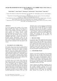
Amazon<br />
Corresponding stddev. on<br />
interferometry<br />
Microwaves and Radar Institute
Combined estimation: <strong>the</strong>ory<br />
Varying ionosphere<br />
Ω<br />
N<br />
�<br />
�<br />
�11�1�TEC Satellite orbit<br />
Mean -> FR<br />
Slant -> shift<br />
�TEC<br />
12<br />
� � 2<br />
�x<br />
L N �1�<br />
�<br />
eB �κˆ<br />
� � �<br />
cmf<br />
2<br />
0<br />
�<br />
�<br />
L<br />
Divide Ionosphere<br />
into N segments<br />
6<br />
Coherent length = L<br />
TEC1 TEC2 3<br />
�<br />
TEC � 1<br />
2<br />
Measure of FR Measure of Azimuth shift<br />
TEC � TECN<br />
� �T TEC TEC � TEC<br />
�12�N� �<br />
TEC<br />
� � C<br />
� � E T 1 1 1 �<br />
N �1<br />
�<br />
N<br />
Microwaves and Radar Institute
Combined estimation: estimation (phase and coherence)<br />
�<br />
� Ω � �G<br />
� ��<br />
� �<br />
� �<br />
�<br />
� Δa<br />
� � 0<br />
Ω<br />
G<br />
0<br />
Δa<br />
TEC � �<br />
�<br />
�<br />
�<br />
�<br />
�<br />
TEC � C d<br />
Coherence comparison:<br />
Equation to be solved<br />
Solution:<br />
�a by 3-ways<br />
� � � �<br />
T �1<br />
�1<br />
T �1<br />
G C G G<br />
D<br />
D<br />
obs<br />
Interferometric<br />
phase correction<br />
FR only Combined<br />
Microwaves and Radar Institute
Tomography: test<br />
Geometry of problem<br />
Height<br />
We used azimuth sub-look parallax.<br />
a priori posterior<br />
Azimuth<br />
Observation<br />
a prior<br />
posterior<br />
Azimuth<br />
Range<br />
Microwaves and Radar Institute
Conclusion<br />
Adversary<br />
effects<br />
<strong>Pol</strong>arimetry FR estimation<br />
Correction approach<br />
Azimuth shift Image correlation and resampling<br />
Interferometric<br />
(Limit)<br />
(Limited to quad-pol)<br />
phase From �TEC estimation (Still remaining azimuth drift)<br />
• The combined estimator per<strong>for</strong>ms better.<br />
Using �FR and/or �FR + azimuth shift<br />
(No way of getting ground truth)<br />
• The parametric estimation can be extended to 3rd dimension.<br />
• What can we do with single-pol interferometric phase, or tropical <strong>for</strong>est<br />
(<strong>BIOMASS</strong>) of Equator?<br />
Microwaves and Radar Institute