Analyst® 1.6 Software Scripts User Guide - AB Sciex

Analyst ® 1.6 Software 

Scripts User Guide 

Release Date: August 2011

This document is provided to customers who have purchased 

AB SCIEX equipment to use in the operation of such AB SCIEX 

equipment. This document is copyright protected and any reproduction 

of this document or any part of this document is strictly prohibited, 

except as AB SCIEX may authorize in writing. 

Software that may be described in this document is furnished under a 

license agreement. It is against the law to copy, modify, or distribute 

the software on any medium, except as specifically allowed in the 

license agreement. Furthermore, the license agreement may prohibit 

the software from being disassembled, reverse engineered, or 

decompiled for any purpose. 

Portions of this document may make reference to other manufacturers 

and/or their products, which may contain parts whose names are 

registered as trademarks and/or function as trademarks of their 

respective owners. Any such usage is intended only to designate 

those manufacturers' products as supplied by AB SCIEX for 

incorporation into its equipment and does not imply any right and/or 

license to use or permit others to use such manufacturers' and/or their 

product names as trademarks. 

AB SCIEX makes no warranties or representations as to the fitness of 

this equipment for any particular purpose and assumes no 

responsibility or contingent liability, including indirect or consequential 

damages, for any use to which the purchaser may put the equipment 

described herein, or for any adverse circumstances arising therefrom. 

For research use only. Not for use in diagnostic procedures. 

The trademarks mentioned herein are the property of 

AB Sciex Pte. Ltd. or their respective owners. 

AB SCIEX is being used under license. 

AB SCIEX 

71 Four Valley Dr., Concord, Ontario, Canada. L4K 4V8. 

AB SCIEX LP is ISO 9001 registered. 

© 2011 AB SCIEX. 

Printed in Canada.

Contents 

Foreword. . . . . . . . . . . . . . . . . . . . . . . . . . . . . . . . . . . . . . . . . . . . . . . . . . . . . . . . . . 5 

Related Documentation . . . . . . . . . . . . . . . . . . . . . . . . . . . . . . . . . . . . . . . . . . . . .5 

Technical Support . . . . . . . . . . . . . . . . . . . . . . . . . . . . . . . . . . . . . . . . . . . . . . . . .5 

Analyst Software Scripts. . . . . . . . . . . . . . . . . . . . . . . . . . . . . . . . . . . . . . . . . . . . . 7 

Related Documentation . . . . . . . . . . . . . . . . . . . . . . . . . . . . . . . . . . . . . . . . . . . . .7 

Installing or Uninstalling Scripts . . . . . . . . . . . . . . . . . . . . . . . . . . . . . . . . . . . . . .7 

Add Missing Zeros . . . . . . . . . . . . . . . . . . . . . . . . . . . . . . . . . . . . . . . . . . . . . . . .8 

Add Normalized ADC Traces . . . . . . . . . . . . . . . . . . . . . . . . . . . . . . . . . . . . . . . .9 

Analyst 1.2 Peak Finder Parameters . . . . . . . . . . . . . . . . . . . . . . . . . . . . . . . . .10 

Batch Script Driver . . . . . . . . . . . . . . . . . . . . . . . . . . . . . . . . . . . . . . . . . . . . . . .11 

Change All Methods . . . . . . . . . . . . . . . . . . . . . . . . . . . . . . . . . . . . . . . . . . . . . .13 

Convert Methods . . . . . . . . . . . . . . . . . . . . . . . . . . . . . . . . . . . . . . . . . . . . . . . . .14 

Creating Quantitation Methods and Text Files . . . . . . . . . . . . . . . . . . . . . . . . . .15 

DBS Settings . . . . . . . . . . . . . . . . . . . . . . . . . . . . . . . . . . . . . . . . . . . . . . . . . . . .21 

Define Custom Elements . . . . . . . . . . . . . . . . . . . . . . . . . . . . . . . . . . . . . . . . . .23 

Delete Others . . . . . . . . . . . . . . . . . . . . . . . . . . . . . . . . . . . . . . . . . . . . . . . . . . .26 

DFT Tracker . . . . . . . . . . . . . . . . . . . . . . . . . . . . . . . . . . . . . . . . . . . . . . . . . . . .27 

Export IDA Spectra . . . . . . . . . . . . . . . . . . . . . . . . . . . . . . . . . . . . . . . . . . . . . . .28 

Export Sample Information . . . . . . . . . . . . . . . . . . . . . . . . . . . . . . . . . . . . . . . . .30 

Export to JCamp . . . . . . . . . . . . . . . . . . . . . . . . . . . . . . . . . . . . . . . . . . . . . . . . .31 

IDA Trace Extractor . . . . . . . . . . . . . . . . . . . . . . . . . . . . . . . . . . . . . . . . . . . . . . .33 

Label Selections . . . . . . . . . . . . . . . . . . . . . . . . . . . . . . . . . . . . . . . . . . . . . . . . .40 

Label XIC Traces . . . . . . . . . . . . . . . . . . . . . . . . . . . . . . . . . . . . . . . . . . . . . . . .41 

Make Exclusion List from Spectrum . . . . . . . . . . . . . . . . . . . . . . . . . . . . . . . . . .42 

Make Subset File . . . . . . . . . . . . . . . . . . . . . . . . . . . . . . . . . . . . . . . . . . . . . . . .43 

Manually Integrate . . . . . . . . . . . . . . . . . . . . . . . . . . . . . . . . . . . . . . . . . . . . . . .45 

Mascot . . . . . . . . . . . . . . . . . . . . . . . . . . . . . . . . . . . . . . . . . . . . . . . . . . . . . . . . .48 

Mass Defect Filter . . . . . . . . . . . . . . . . . . . . . . . . . . . . . . . . . . . . . . . . . . . . . . . .52 

Merge MRM . . . . . . . . . . . . . . . . . . . . . . . . . . . . . . . . . . . . . . . . . . . . . . . . . . . .54 

MRM3 Optimization Script . . . . . . . . . . . . . . . . . . . . . . . . . . . . . . . . . . . . . . . . .55 

Multiple Batch Scripts . . . . . . . . . . . . . . . . . . . . . . . . . . . . . . . . . . . . . . . . . . . . .65 

Open In Workspace . . . . . . . . . . . . . . . . . . . . . . . . . . . . . . . . . . . . . . . . . . . . . .66 

Peak List from Selection . . . . . . . . . . . . . . . . . . . . . . . . . . . . . . . . . . . . . . . . . . .67 

Regression Calculator . . . . . . . . . . . . . . . . . . . . . . . . . . . . . . . . . . . . . . . . . . . . .68 

Remove Graph Selections . . . . . . . . . . . . . . . . . . . . . . . . . . . . . . . . . . . . . . . . .69 

Repeat IDA Method . . . . . . . . . . . . . . . . . . . . . . . . . . . . . . . . . . . . . . . . . . . . . . .70 

Savitzky-Golay Smooth . . . . . . . . . . . . . . . . . . . . . . . . . . . . . . . . . . . . . . . . . . . .71 

Selection Average and Standard Deviation . . . . . . . . . . . . . . . . . . . . . . . . . . . .72 

Send to ACD SpecManager . . . . . . . . . . . . . . . . . . . . . . . . . . . . . . . . . . . . . . . .73 

Signal-to-Noise Using Peak-to-Peak . . . . . . . . . . . . . . . . . . . . . . . . . . . . . . . . . .75 

Signal-to-Noise Using Standard Deviation . . . . . . . . . . . . . . . . . . . . . . . . . . . . .76 

Split Graph Script . . . . . . . . . . . . . . . . . . . . . . . . . . . . . . . . . . . . . . . . . . . . . . . .77 

Subtract Control Data from Sample Data . . . . . . . . . . . . . . . . . . . . . . . . . . . . . .78 

Unit Conversion . . . . . . . . . . . . . . . . . . . . . . . . . . . . . . . . . . . . . . . . . . . . . . . . . .79 

Release Date: August 2011 3

Contents 

Wiff To MatLab . . . . . . . . . . . . . . . . . . . . . . . . . . . . . . . . . . . . . . . . . . . . . . . . . .80 

XIC from BPC . . . . . . . . . . . . . . . . . . . . . . . . . . . . . . . . . . . . . . . . . . . . . . . . . . .84 

XIC from Table . . . . . . . . . . . . . . . . . . . . . . . . . . . . . . . . . . . . . . . . . . . . . . . . . .85 

4 Release Date: August 2011

Foreword 

This guide provides information on how to use the Analyst ® software scripts and is intended for 

customers and FSEs. 

Related Documentation 

The guides and tutorials for the instrument and the Analyst ® software are installed automatically 

with the software and are available from the Start menu: All Programs > AB SCIEX > Analyst. A 

complete list of the available documentation can be found in the online Help. To view the Analyst 

software Help, press F1. 

Technical Support 

AB SCIEX and its representatives maintain a staff of fully-trained service and technical 

specialists located throughout the world. They can answer questions about the instrument or any 

technical issues that may arise. For more information, visit the Web site at www.absciex.com. 


Foreword 


Analyst Software Scripts 

The purpose of this document is to explain how to install and use Analyst ® software scripts. It 

also provides an overview of the uses of each script and how to uninstall a script, if required. 

Related Documentation 

You can also create your own scripts using the Visual Basic Version 6 program. For more 

information, see the Analyst ® Software Automation Cookbook: A guide to controlling Analyst ® 

software version 1.6 from Visual Basic .NET Version Visual Studio-2005. 

Installing or Uninstalling Scripts 

Some scripts are automatically installed when the Analyst software is installed. The remaining 

scripts are available in the Scripts folder. When you have decided which scripts you want to use, 

use the following procedure to install them. 

Note: This guide contains the scripts for all instruments and different software 

versions. To determine which scripts the software version installed on your instrument 

supports, see the Analyst software release notes. 

Installing a Script 

1. Navigate to the following folder on your workstation: :\Program 

Files\Analyst\Scripts. 

2. Open the required folder, open the script folder, and then double-click 

ScriptRunner.exe. 

3. Follow the on-screen instructions to install the scripts. 

The script is available on the Script menu. 

Uninstalling a Script 

Note: For some scripts, if you hold down the Shift key while accessing a 

script on the Script menu, a description of the script is displayed. 

• To uninstall a script, do one of the following: 

• For processing scripts, navigate to the :\Analyst Data\Projects\API 

Instrument\Processing Scripts folder and then delete the script .dll or, if 

applicable, .exe and .bmp files, manually. 

• For acquisition scripts, navigate to the :\Analyst Data\Projects\API 

Instrument\Acquisition Scripts folder and then delete the script .dll or, if 

applicable, .exe and .bmp files, manually. 



Add Missing Zeros 

Use this script to add a value of zero intensity for the missing mass values in the spectrum. To 

minimize storage requirements and to speed data display and processing, the Analyst ® software 

does not store or display spectral points with an original intensity of zero. If required, for example, 

when exporting a spectrum for subsequent processing by custom software, you can add these 

data points back to the spectrum. 

To use the script 

• Click the spectrum and then click Script > Add Missing Zeros. 

The script will add the zero values to all missing masses in the current spectrum. 


Add Normalized ADC Traces 


Use this script to overlay the active chromatogram or chromatograms with normalized ADC data 

from a corresponding data file. Run the script when a pane containing one or more 

chromatograms is active in Explore mode. There may be a time region selected in a trace. If no 

selection is made, then the entire chromatogram is overlayed. 

In case that several ADC traces are part of the .wiff file, all of them will be displayed. 

Notes 

• If the data in the active pane came from several samples, then the ADC data for the 

sample corresponding to the first data set (not the active data set) is shown. 


• Do one of the following: 

• Click Script > AddNormalizedADC. 

• To see the script description and add ADC data to an active Explore pane, 

hold the Shift key down while clicking the script. 



Analyst 1.2 Peak Finder Parameters 

The Analyst ® software uses an improved version of Peak Finder for better peak detection and ion 

abundance measurement. If you are using the Peak Finder algorithm to analyze .wiff files that 

were acquired using the Analyst software, then you can use this script to set the peak finder 

algorithm parameters. 

To install the script 

• Make sure that the Analyst Data\Projects\API Instrument\Processing Scripts folder 

contains the Analyst12PeakFinderParams.dll. 


Note: This script is installed automatically when the Analyst 1.6 software 

is installed. There is no separate installation program for it. 

1. Click Script > Analyst12PeakFinderParams. 

The Analyst 1.2 Peak Finder Algorithm Parameter dialog appears. 

2. To activate the Analyst 1.2 version of Peak Finder, select the Use Analyst 1.2 peak 

finder algorithm for Analyst 1.2 files check box. 

3. Do the following: 

• In the Intensity Threshold (%) field, type the value, as a percentage, of the 

minimum intensity required to distinguish between noise and peak. 

• In the Centroid Height (%) field, type the value, as a percentage, to be used 

by the centroiding algorithm to find the peak and to determine the centroid m/z 

value at this percentage height. 

• In the Centroid Peak Width (min) field, type the minimum value, in ppm, to 

be used by the centroiding algorithm to find the peak width and to determine 

the centroid m/z value at this width. 

• In the Centroid Peak Width (max) field, type the maximum value, in ppm, to 

be used by the centroiding algorithm to find the peak width and to determine 

the centroid m/z value at this width. 

• In the Centroid Merge Distance (amu) field, type a value, in amu, to be used 

to determine whether two centroid peaks should be merged into one. If two 

peaks are within this tolerance, then they will be merged together. 

• In the Centroid Merge Distance (ppm) field, type a value, in ppm, to be used 

to determine whether two centroid peaks should be merged into one. If two 

peaks are within this tolerance, then they will be merged together. 

4. Click OK. 

5. To return to the Analyst 1.4.1 Peak Finder algorithm, clear the Use Analyst 1.2 peak 

finder algorithm for Analyst 1.2 files check box. 


Batch Script Driver 


With the Batch Acquisition Script Driver, you can run an acquisition script on multiple data files 

(.wiff) by attaching the acquisition script to a batch that is submitted to the queue. These scripts 

are used to immediately process the data either after a sample completes or after the batch 

finishes. The script will process the data files as if they were separate batches submitted to the 

queue. Occasionally, you might need to apply these acquisition scripts on previously acquired 

data because either the script did not exist at the time of acquisition or a rerun of the script is 

required. 


1. Navigate to C:\Program Files\Analyst\bin and then double-click 

BatchScriptDriver.exe. 

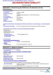
Figure 1-1 Batch Acquisition Script Driver dialog 

2. To select an acquisition script, click Select. 

3. To add a data file, click Add File. Click Add Folder to add an entire folder of data 

files. 

4. To remove a data file, select it from the list and then click Remove Selected. Click 

Remove All to remove all the data files. 

5. To process some of the samples contained in a .wiff data file, select the Process 

Limited Sample Number Range check box. This field is available only if you have 

selected only one data file to process. 

6. In the from sample and to fields, type the sample number range to be processed. 



7. To run the script on each data file in the list, click Run. 

8. To stop the script, click Close. 


Change All Methods 


It is often necessary to change the ion source conditions of a method, particularly with the 

NanoSpray ® ion source after changing the emitter tip. This script modifies every method in a 

selected project with new values for IonSpray Voltage (IS), Ion Source Gas 1 (GS1), and 

Interface Heater Temperature (IHT). 

Note: This script is used with any QTRAP ® system. It is not used by QSTAR ® 

instruments. 


1. Click Script > change all methods. 

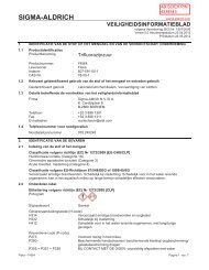
Figure 1-2 Change All Methods dialog 

2. Select a project containing the methods that you want to modify. 

3. Select the parameters that you want to change. If the parameter is not in the method 

file, it will be ignored. 

4. Type a value for positive experiments. 

5. Type a value for negative experiments. 

6. Select the update method with current instrument settings check box if you want 

to change the AF3, EXB, and C2B parameters for all the methods in the selected 

project. 

7. Click Change All. 



Convert Methods 

Use this script to convert methods from one type of instrument to another. The script converts the 

method to the currently active hardware profile, using appropriate values for each parameter. 

Only the ion source and compound dependent parameters for mass ranges and experiments are 

shown. 

The Convert Methods script automatically optimizes mass ranges and, in addition to single 

period, single experiment methods, converts multiple periods, multiple experiments, and IDA 

criteria. 

Prerequisites 

• .Net framework 3.5 SP2 (will be automatically installed if required) 

To install the script 

• To install the script, navigate to the :\Program Files\Analyst\Scripts\Convert 

Methods folder and then double-click Convert Methods Setup.exe. 


Make sure a hardware profile is active. 

1. Click Script > Convert Methods. 

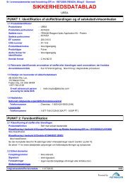
Figure 1-3 Convert Methods dialog 

2. Click Open, navigate to the method that you want to convert, and then click Open. 

The Method Converter dialog displays the instrument name of the original method. 

3. Click Save, type a name for the converted method, and then click Save. 



Creating Quantitation Methods and Text Files 

The Create Text File From Quan Method script exports a quantitation method to a tab-delimited 

text file. The Create Quan Method From Text Files script imports the information contained in a 

tab-delimited text file to a Quantitation Method File (.qmf). Currently, the Quantitation Method 

component in the Analyst ® software does not support this functionality. 

The Create Text File from Quan Method script creates a text file representation of a quantitation 

method file. A column in the text file is created only for all of the required fields. The optional 

fields will be created if the field value is not the same for all peaks in the quantitation method. 

The Create Quan Method From Text Files script specifies the default values for any of the nonrequired 

fields in the text file such as integration algorithm or regression parameters. For more 

information, see Text File Format on page 17. 

To use the Create Quan Methods From Text Files script 

1. Click Script > Create Quan Methods From Text Files. 

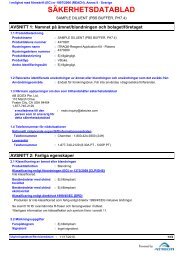
Figure 1-4 Create Quantitation Methods from Text Files dialog 



2. Use the parameters in the Default Generic Parameters group to create a 

quantitation method. The Algorithm, Extraction Type, Period, and Experiment 

fields are not available in the Analyst software. Set the following parameters as 

required: 

• In the Algorithm drop-down list, select a peak-finding algorithm. The Window 

Summation algorithm sums all the intensities in the retention threshold and will 

not find any peaks. 

• In the Extraction Type drop-down list, select the type of data that will be 

integrated. 

• In the Period and Experiment drop-down lists, select the period number and 

experiment number. 

The Default Analyst Classic Parameters, Default General IntelliQuan Parameters, 

Default IntelliQuan MQ III Parameters, and the Default Window Summation 

Parameters groups contain the parameters that are used by the algorithm selected 

in the Algorithm field. 

Note: The Smoothing Width field in the Default General IntelliQuan 

Parameters group is half the smoothing width. 

3. Select the Use Baseline Subtraction check box to have the Window Summation 

algorithm sum the intensities to the horizontal line at the minimum intensity of the 

data points within the summation window, as opposed to summing down to the 

intensity zero. 

4. In the Regression Parameters group, select the regression information. The 

information specified here is applied to every analyte peak. Unlike the previous 

parameters, it is not possible to indicate this information in the text files; therefore, 

the same regression parameters are applied to all analytes. For a full description of 

the parameters, see the Help. 

5. To create one quantitation method, click Create One Method and then navigate to 

the text file that will be used to create the quantitation method. 

6. To create multiple methods from multiple text files, click Create Multiple Methods 

and then navigate to the folder. A quantitation method is created for each text file in 

this folder. 

To use the Create Text File from Quan Method script 

1. Create and save a quantitation method in the Analyst software. 

2. Click Script > Create Text File from Quan Method. 


s. 

Figure 1-5 Options dialog 

3. Select the Export all columns check box and then click OK. 

4. Navigate to and select the quantitation method file (.qmf). 

5. Navigate to and select the location of the text file. 

The script will generate the text file. 

Text File Format 


The text files used to create the quantitation methods (Create Quan Methods from Text Files) and 

generated from the methods (Create Text File from Quan Method) are in the following format: 

• Separate the various fields with tab characters and end each line with a carriage 

return / line feed characters. 

• The very first row of the file should contain column headings. All of the columns 

shown in the following table marked as Required must be present; the remaining 

columns are optional. The actual order of the columns is not important. 

• Each subsequent line should contain the information as shown in the table for either 

one analyte or an internal standard peak. 

Table 1-1 Text File Formats 

Column name Required Description 

Peak Name Yes The name of the analyte or internal standard peak. 

First Mass Yes For MRM data, the Q1 mass for the peak; for full-scan data, 

the starting mass for the XIC to integrate; for Q1 MI or Q3 

MI data, the mass. 

Second Mass Maybe This field is required when integrating full-scan or MRM 

data, but not for Q1 MI or Q3 MI data. For MRM data, this is 

the Q3 mass for the peak; for full-scan data, it is the ending 

mass for the XIC to integrate. 

Extraction Type No The type of data to integrate. If present, this should be one 

of: 

0 – MRM data 

1 – Q1 MI or Q3 MI data 

2 – full-scan data 



Table 1-1 Text File Formats (Continued) 


Is IS No Specifies whether the current peak is an internal standard or 

an analyte. Select Yes if the peak is an internal standard; 

otherwise select No. If this column is not present, then all 

peaks defined are assumed to be analytes. 

Note: Internal standard peaks should be defined first in the 

text file before any analyte peaks that use that IS. 

IS Name No For analyte peaks, specifies the name of the corresponding 

internal standard (if any). If a given analyte will not use an 

internal standard, leave the contents of this field empty. For 

internal standard peaks themselves, the contents of this 

field are ignored. 

Period No The period number for the peak (from 1 to the number of 

periods in the data). 

Experiment No The experiment number for the peak (from 1 to the 

maximum number of experiments in the period). 

Use Relative RT No For analyte peaks that are using an internal standard, 

specifies whether or not the expected retention time is 

relative to that of the IS. Select Yes if so; otherwise, select 

No. The contents of this field are ignored for other peaks, 

but must still contain either Yes or No. 

Conc Units No The concentration units. 

Calc Conc Units No The calculated concentration units. 

Bkg Start No Start time in minutes for the peak background. Note that this 

parameter does not affect the peak integration in any way, 

however it does affect how the noise (and hence S/N) is 

calculated. 

Bkg End No End time in minutes for the peak background. 

Expected RT No The expected retention time in minutes (from 0 to 1666). 

RT Window No The retention time window in seconds (from 1 to 1000). 

Algorithm No Specifies which peak-finding and integration algorithm 

should be used. If present, this should be one of: 

0 – Analyst Classic (TurboChrom) 

1 – IntelliQuan - IQA II (Automatic) 

2 – IntelliQuan – MQ III 

3 – Window Summation 

Note that the window summation algorithm is not available 

from within the Analyst software user interface, but can be 

enabled using the script. 

Bunching Factor No The bunching factor for the peak (from 1 to 100) when using 

the TurboChrom algorithm. 

Num Smooths No The number of smooths (from 0 to 10) when using the 

TurboChrom algorithm. 


Table 1-1 Text File Formats (Continued) 



Noise Threshold No The noise threshold (from 1 -6 to 1 9 ) when using the 


Area Threshold No The area threshold (from 1-6 to 112 ) when using the 


Separation Width No The separation width (from 0 to 5) when using the 


Separation Height No The separation height (from 0 to 1) when using the 


Exp Peak Ratio No The exponential peak ratio (from 1 to 16 ) when using the 


Exp Adjusted 

Ratio 

No The exponential adjusted ratio (from 2 to 1 6 ) when using the 


Exp Valley Ratio No The exponential valley ratio (from 1 to 1 6 ) when using the 


Min Height No The minimum allowed peak height (from 0 to 116 ) when 

using the IntelliQuan algorithm. 

Min Width No The minimum allowed peak width (from 0 to 1 16 ) in seconds 

when using the IntelliQuan algorithm. 

Smooth Width No The half-width of the Savitzky-Golay smoothing filter (from 0 

to 20) when using the IntelliQuan algorithm. 

MQ III Noise 

Percent 

MQ III Baseline 

Sub Window 

MQ III Peak 

Splitting Factor 

No The noise percentage when using the MQ III option of the 

IntelliQuan algorithm. This should be an integer from 0 to 

100. 

No The baseline subtraction window (from 0 to 10 minutes) 

when using the MQ III option of the IntelliQuan algorithm. 

No The peak-splitting factor (from 0 to 10) when using the MQ 

III option of the IntelliQuan algorithm. 

MQ III Use Largest No When using the MQ III option of the IntelliQuan algorithm, 

specifies whether the largest peak (within the retention time 

window) or the peak whose retention time is closest to that 

expected is reported. Select Yes to use the largest peak and 

No to use the closest. 

Summation 

Baseline Sub 

No When using the special window summation algorithm, 

specifies whether the area should be integrated to the 

intensity=0 line or to the intensity value of the least intense 

data point within the window. 

The following table shows an example text file for full-scan data. Imagine that there are tabs 

between the columns and a hard return at the end of each line. 

Table 1-2 Example Text File for Full-Scan Data 

Peak Name First Mass Second Mass Bunching Factor 

Analyte Peak 1 500.10 500.70 1 



Table 1-2 Example Text File for Full-Scan Data (Continued) 

Peak Name First Mass Second Mass Bunching Factor 

Analyte Peak 2 812.00 813.00 2 

Analyte Peak 3 400.00 401.00 3 

The following table shows one more example for MRM data. The Analyte Peak 1 will be set up to 

use the specified internal standard and Analyte Peak 2 will not use an internal standard. 

Table 1-3 Example Text File for MRM Data 

Peak Name Is IS IS Name First Mass Second Mass 

IS Peak 1 Yes 500.10 413.20 

Analyte Peak 1 No IS Peak 1 600.20 382.10 

Analyte Peak 2 No 400.00 312.1 

The following table contains a mixture of full-scan and MRM data in different experiments: 

Table 1-4 Example Text File for MRM Data 

Peak Name Extraction 

Type 

Experiment First Mass Second Mass 

Analyte Peak 1 0 1 500.10 413.20 

Analyte Peak 2 0 1 600.20 382.10 

Analyte Peak 3 2 2 812.00 813.00 

Analyte Peak 4 2 2 400.00 401.00 


DBS Settings 


The DBS (Dynamic Background Subtraction algorithm) is a feature that ensures better 

selection of precursor ions in an IDA (Information Dependant Acquisition) experiment. When 

DBS is activated, IDA uses a spectrum that has been background subtracted to select the 

candidate ion of interest for MS/MS analysis, as opposed to selecting the precursor from the 

survey spectrum directly. DBS enables detection of species as their signal increases in intensity, 

thus focusing on detection and analysis of the precursor ions on the rising portion of the LC peak, 

up to the top of the LC peaks (maximum intensity). 

The DBS functionality is embedded in the Analyst ® 1.6 software for IDA experiments; however, 

the associated parameters are not accessible in the Analyst software. The hidden parameters 

and their default values are as follows: 

• Average number of previous spectra = 4 

• Smooth before subtract: activated 

• Smooth = 5 data points. 

Use this script to change the default parameters to ones that are more representative of the 

experimental conditions. Depending on the cycle time and chromatography, the default settings 

may result in an obvious candidate ion from being omitted for dependent MS/MS analysis or the 

same candidate ion may be selected for MS/MS analysis over the entire LC peak. Therefore, this 

script will be useful to customers who find that the embedded default values are not appropriate 

for their analysis. 

After the script is installed, the DBS feature uses the settings in the script. The script will 

remember the last settings used. 

Prerequisites 

• Analyst 1.6 Software installed 

• Administrator rights on the computer 


1. Activate the DBS feature by selecting the After Dynamic Background Subtraction 

of Survey scan check box on the IDA – First Level Criteria tab. 



2. Although the DBS feature is activated at the method level, the DBS options are set 

using the script. From the Analyst software menu, click Script > DBS Settings. 

• Subtract the _ previous spectra from current spectrum: Use this field to 

select the number of spectra averaged to represent the background signal. 

These spectra are taken immediately before the current survey spectrum. 

Typical values used are between 2 and 5. 

• Smooth Before Subtract: Select to make sure that the current survey 

spectrum is smoothed using a Savitzky-Golay smooth before the subtraction 

step. Select the number of points to consider in the process. A typical value is 

5. 

Survey Scans Supported 

The DBS feature can be used with any IDA survey scans currently supported: EMS, EMC, 

Precursor Scan, Neutral Loss, MRM, Q3 MS and Q3 MI. DBS does not apply to the confirmation 

or dependant levels. 

Known Limitations and Issues 

• With the exception of DBS being on or off, DBS parameters are not stored as part of 

the file information. In order to recall which settings were used, the user should 

document the parameters selected during the acquisition. 

• DBS is meant for use during LC analysis, therefore, when performing IDA by infusion 

it is recommended to have DBS deactivated. 


Define Custom Elements 


Use this script to select a custom isotope pattern when working with radio-labeled compounds. 

An experiment-specific element pattern is used in the data interpretation in conjunction with the 

Analyst ® software calculators or the Metabolite ID application. 

The custom isotope patterns are stored together with the information from the periodic table 

elements in the element definition file, SAElements.ini, which is located in the Analyst\bin folder. 

In the element definition file, the custom elements must have a unique symbol and an atomic 

number of 104 or higher. 

Prerequisites 

The following program is optional: 

• Metabolite ID 1.3 for Analyst QS 2.0 software 

When the script is launched for the first time, a backup copy of the SAElements.ini file is saved in 

the API Instrument folder. If needed, the edited SAElements.ini file in Analyst\bin folder can be 

replaced with this file. 

To update the element definition file successfully 

1. Do not open the SAElements.ini file in another text editor program while using the 

software. 

2. Make sure the file access must be set to read/write. 

To edit the Define Custom Elements table 

The custom element table cannot be edited in the dialog. After the element definition file is 

updated, the custom elements can be used with the Analyst software calculators. 

1. Click Script > DefineCustomEl. 



Figure 1-6 Define Custom Elements dialog 

2. In the table, click the row containing the element. 


3. 

Figure 1-7 Define Element dialog 

Edit the fields and then click OK. 

4. To save the updated element definition file and exit the program, click OK. 


To view the custom element symbol, custom element name, and custom pattern 

• To view the custom pattern in the mass/relative intensity graph, in the Define 

Custom Elements dialog, click Show. 

The Iosotopic Distribution dialog appears. 

The total of the individual isotope abundance for an element stored in the element 

definition file must be equal to one. Therefore, the abundances entered in the Define 

Element Window are rescaled before they are added to the Define Custom Elements 

dialog. This Isotopic Distribution dialog cannot be edited. You can zoom in the area 

of interest by dragging along the corresponding x- or y-axis region. 

The application requires the gen01.wiff example file to display custom pattern. If the 

gen01.wiff file is not in the Example folder in the Analyst Data\Projects folder, you will 

be prompted to find this file. 



Delete Others 

Use this processing script to delete all panes except for the active one. 


1. With a sample file (.wiff) with multiple panes open, click a pane. 

The pane becomes the active pane. 

2. Click Script > DeleteOthers. 

All the panes except for the active one are deleted. 


DFT Tracker 


The Dynamic Fill Time (DFT) Tracker script tracks the DFT settings used during QTRAP ® 

instrument scans. You can use the script to determine the optimal fill time for linear ion trap (LIT) 

mode to obtain high data quality over a wide dynamic range. The DFT Tracker monitors the 

following LIT scan types: Enhanced MS (EMS), Enhanced Resolution (ER), Enhanced Product 

Ion (EPI), and MS/MS/MS (MS3). 


• Click Script > DFTTracker. 

Figure 1-8 Dynamic Fill Time Tracker dialog 

DFT Tracker monitors the dynamic changes occurring during a real-time run. 

The system dynamically calculates the time required to fill the linear ion trap. For 

abundant compounds, a short fill time reduces the space charge effects by limiting 

the number of ions in the ion trap; on the other hand the longer fill time increases 

weak signals by allowing the ions to accumulate. 



Export IDA Spectra 

Use this script to export data in a format that can be searched using a third-party application. The 

Export IDA Spectra script exports every dependent product spectrum from an IDA (Information 

Dependent Acquisition) LC/MS run to a series of text files. These text files can then be submitted 

and searched using Sequest. The export is optimized so that any spectra in adjacent cycles with 

the same precursor m/z are combined into a single spectrum. This optimization also applies to 

spectra with the same precursor but which reside in different experiments, most likely using 

different values of the collision energy. 

The charge state of the precursor ion is a required input. Sequest tries to automatically determine 

this from the isotope spacing at the precursor m/z in the IDA survey spectrum. Note that while 

this determination is usually correct, it is not always so. 


It is assumed that the first experiment of the IDA method represents the survey spectrum and 

that all other experiments represent dependent product spectra. Therefore, this script cannot be 

used if there are multiple survey experiments. 

1. With an IDA chromatogram in an active pane, click Script > Export IDA Spectra. 

Figure 1-9 Export IDA Spectra (in Sequest Format) dialog 

2. In the Mass tolerance for combining MS/MS spectra field, type the tolerance to be 

used to determine if two precursor m/z values should be considered identical. If the 

precursors for two sequential product spectra differ by less than this value, the 

spectra are added and a single text file is exported. 

3. In the MS/MS intensity threshold field, type the threshold that is applied to each 

product spectrum after it is centroided. It is assumed that peaks below this threshold 

are most likely noise. Type 0 in the field if you do not want to use a threshold. 

4. In the Minimum number of MS/MS ions for export field, type the minimum number 

of ions that must be present in a product spectrum, after centroiding and 

thresholding, in order for a text file to be exported. If a spectrum does not contain the 

specified number of ions, it is assumed that the quality of the spectrum is too low to 

merit exporting. 



5. To separate fields in the output files with a space character, select the Separate 

values in output with a space, not a tab check box; otherwise a tab character is 

used. (Certain versions of Sequest require a space delimiter.) 

6. To export the text files, click Go. 

7. In the Save As dialog, type a location and root file name for the exported text files. 

Before being exported to a text file, each of the product spectra is centroided. The 

cycle number range and charge state is appended to this file for each exported 

spectrum. 



Export Sample Information 

Use this script to extract sample information, such as the name, sample ID, comment, and 

acquisition method name for all samples in the .wiff file. You can define the information you would 

like exported, and the script saves the information in an .inf file located in the same folder as the 

.wiff file. 


1. With a chromatogram or spectrum in an active pane, click Script > 

ExportSampleInformationFromMultipleSampleinOneWiff while pressing the Ctrl 

key. 

Figure 1-10 Export Sample Information dialog 

2. Select the check boxes that correspond to the information that you want to export 

and then click OK. 


Export to JCamp 


You can use the Analyst ® software to export graph data to a tab-delimited text file that can be 

read by most applications; however, some applications require a more specific format. 

With the Export to JCAMP script, you can export graph data in the JCAMP format. The script 

works on both chromatograms and spectra. For chromatograms, depending on the number of 

selections made, either all the spectral data of the chromatogram is exported, or the averaged 

sum of the selected regions is exported. If you are using this script on a single spectrum, then 

only that data is exported. This script can also be attached to a batch so that the export occurs 

automatically after the sample is acquired. 

Table 1-5 shows an overview of the operation of the script. When run interactively the exact 

behavior depends on the active Analyst software data. 

Table 1-5 Script Operation 

Modes Active data Operation 

Interactive Spectrum You will be prompted for the name of the JCamp file and 

the active spectrum exported to it. 

Interactive Chromatogram with 

two or more 

selections 

Interactive Chromatogram with 

one or no selections 


You will be prompted for the name of the JCamp file and an 

averaged spectrum corresponding to each of the 

chromatogram’s selections exported to it. 

You will be prompted for the name of the JCamp file and 

every spectrum for the run exported to it. 

Batch N / A The name of the JCamp file is generated by appending the 

sample number to the name of the .wiff file and changing 

the extension to jdx. Every spectrum for the run is exported 

to the JCamp file. For multiple period/experiment data, a 

separate file is exported for each experiment (the period 

and experiment numbers are appended to the filename). 

1. To use the Export to JCAMP do one of the following: 

• With either a chromatogram or a spectrum in an active pane, click Script > 

Export to JCAMP. 

• In the Batch Editor dialog, type Analyst Data \API Instrument\Processing 

Scripts\Export to Jcamp.dll in the Batch Script field. 



Figure 1-11 JCAMP Options dialog 

2. To select the centroiding options, do one of the following: 

• Check the Centroid Exported Spectra check box to centroid the spectra 

before exporting to the JCAMP format. 

• To have the JCAMP Options window appear only if the Ctrl key is pressed 

when clicking the script from the Script menu, or when submitting the batch to 

the queue, select the Only show this dialog again if the control key is 

down check box. 

3. To continue processing and to have the spectrums exported, click OK. 

4. When prompted, type the file name of the exported JCAMP file. When a script is 

attached to the batch, the file name is automatically generated using the following 

format: [WiffFileName]_[Sample#]_[Period#]_[Experiment#].jdx 


IDA Trace Extractor 


Use this script to review the survey data collected using IDA (Information Dependent Acquisition) 

based on the information in the corresponding dependent data. The script searches the MS/MS 

data for given neutral losses or fragments and then calculates the Extracted Ion Chromatograms 

(XICs) for the precursor masses, which give the specified losses or fragments. The XICs are 

overlaid in Explore mode and their peaks are labeled with the precursor mass (Figure 1-12). 

Figure 1-12 Characteristic Traces in Dependent Experiment and XICs of the Survey 

Experiment. The characteristic m/z 387.1 detected in negative mode was converted to m/z 

389.1 in the positive survey scan. 

You can use the script to do the following: 

• Specify a list of expected fragments or neutral losses, in either the positive mode 

polarity, the negative mode polarity or both, in terms of fragment formula or mass. 

• Save the list of masses and fragments for a compound class and load them to the 

settings at a later time. 

• Process just a selected time region in the chromatogram. 

• Display precursor (survey scan) or fragment (dependent scan) XIC trace that yield 

given fragment or neutral loss. 

• From the survey scan chromatograms the user can link to any survey scan 

spectra 

• From the dependent scan traces the user can link to any dependent scan 

spectra 

• Reduce the precursor XIC traces to show just peaks that have corresponding neutral 

losses (or fragments) 

• Save the precursor mass list in a text file for further processing; build the list of 

precursors from a set of samples 

• Save the list of masses in a format that can be loaded to the XICfromTable script 



• Save the list of masses and peaks in a format that can be loaded to the 

CreateQuantMethodFromText script. 

Note: The script is compatible with MRM / MIM IDA data and with the Analyst ® 1.6 

software. 

Note: The script supports parallel data processing from positive and negative 

experiments. Multiple survey and dependent experiments of any polarity can be used. 


Note: The Analyst software version for a specific file can be displayed in the file 

properties > comments. 

1. With a chromatogram of IDA data open in an active pane, click Script > 

IDATraceExtractor. 

You can process a full chromatogram or just a selected region (make a selection 

before running the script). 

Figure 1-13 IDA Trace Extractor dialog 

2. In the Options tab of the script, set the fields as required. For more information, see 

Table 1-6 Tab and Menu Parameters on page 36. 

3. To store the retention times and precursor masses found during processing, click the 

Results tab, type a filename, and then select Save Precursor Information. 



Figure 1-14 IDA Trace Extractor dialog: Results tab 

4. To review or enter the mass information, click the Neutral Losses or Fragments 

tab. Type the neutral losses and fragments as masses or chemical formulas. You 

can also specify the polarity of the Neutral Loss or fragment spectrum experiment 

where the specified neutral loss or fragment is expected to be found. 

Figure 1-15 IDA Trace Extractor dialog: Neutral Losses tab 



Figure 1-16 IDA Trace Extractor dialog: Fragments tab 

5. Click Extract to find the survey XIC traces that give the selected neutral loss or 

fragment. 

6. If the precursor information was saved, the found precursor mass/time data can be 

converted to a compatible format using other scripts. To convert the data, click the 

Results tab and then select the Results File. View and edit this file as required. 

• To make a format for the XICfromTable script, click Make XIC Table. The 

Results File will be converted into a file of the same name with the suffix _XIC. 

• To make a format for the CreateQuantMethodFromText script on the 

Precursor XICs dialog, click Make Quant Input. The Results File will be 

converted into a file of the same name with the suffix _Peaks. 

7. Click File > Save Settings as. Alternatively, previously saved settings can be used. 

Click File > Load Settings to open previously saved settings. 

Several functions are available in the Tools menu. You can start processing without switching to a 

specific tab. 

Table 1-6 Tab and Menu Parameters 

Location Parameters Description 

Neutral Losses Use Masses Select the required neutral loss(es) as 

mass. 

Neutral Losses Use Formulas Select the required neutral loss(es) as 

formula. 

Neutral Losses Start Low mass limit (from mass) for the 

neutral loss(es). 

Neutral Losses End High mass limit (to mass) for the neutral 

loss(es). 


Table 1-6 Tab and Menu Parameters (Continued) 



Neutral Losses Formula Chemical formula of the neutral loss. 

Neutral Losses Extract Start data processing according to the 

current settings. 

Neutral Losses Clear Clear all neutral losses in the settings. 

Neutral Losses Polarity Select the polarity of the Neutral Loss 

experiment where the specified neutral 

loss is expected to be found. 

Fragments Use Masses Describe the characteristic fragment(s) in 

terms of their m/z. 

Fragments Use Formulas Describe the characteristic fragment(s) in 

terms of their formulas. 

Fragments Start Low mass limit (from mass) for the 

fragment m/z window. 

Fragments End High mass limit (to mass) for the 

fragment m/z window. 

Fragments Formula Chemical formula of the fragment 

(protonated/ deprotonated form). 

Fragments Extract Start data processing according to the 

current settings. 

Fragments Polarity Select the polarity of the fragment 

spectrum experiment where the specified 

fragment is expected to be found. 

Fragments Clear Clear all fragments in the settings. 

Options From Time (min) Start of time region to be processed. 

Options To Time (min) End of time region to be processed. 

Options Trace Width (Da) Width of XIC traces in resulting survey 

scan and dependent scan 

chromatograms and mass tolerance 

window for processing in case that the 

neutral losses or fragments are specified 

as chemical formulas. 

Options Remove Unconfirmed Review all peaks in the survey XIC traces 

Peaks 

and retain only those that were validated 

based on the data in corresponding 

dependent scan. 

Options Spectrum Peaks > Minimum size of diagnostic peak in 

dependent scan in terms of signal to 

noise (lowest measurable signal). 

Options Label Peaks > Peak label threshold applied to resulting 

survey and dependent scan 

chromatograms (note that just the largest 

peak in each trace is labeled). 



Table 1-6 Tab and Menu Parameters (Continued) 


Options Show Survey Scan 

Chromatograms 

Options Show Dependent 

Chromatograms 

Options Subtract Peaks Present in 

Control Sample 

Display XICs (original or filtered) from the 

survey scan that correspond to parent 

masses yielding specified fragment or 

neutral loss. 

Display neutral loss traces (one for each 

neutral loss) reconstructed from 

dependent scan data. 

Remove peaks that can be found in the 

control sample XICs from the survey 

scan chromatograms. 

Results Result File Select Results file (containing identified 

peak times and masses will be saved). 

Results Save Precursor 

Information 

Write processing results (list of found 

peaks - times and masses) to selected 

results file. 

Results XIC Peaks > Minimum size of the peak in survey scan 

to be stored in the results file. 

Results Append Results to an 

Existing File 

Do not overwrite existing results file. 

Results View Open the selected results file. 

Results Make XIC Table Use the selected results file to prepare 

settings file for XIC from Table script. 

Results Make Quant Input Use the selected results file to prepare an 

input for CreateQuanMethodFromText 

script. 

File Menu Load Settings… Load previously saved script settings to 

the interface. 

File Menu Save Settings As… Save current script settings for future 

use. 

File Menu Set Results File… See Results/Result File 

Tools Menu Extract Fragments See Fragments/Extract 

Tools Menu Extract Neutral Losses See Neutral Losses/Extract 

Tools Menu Clear Fragments See Fragments/Clear 

Tools Menu Clear Neutral Losses See Neutral Losses/Clear 

Tools Menu Make XIC Table See Results/Make XIC Table 

Tools Menu Make Quant Input See Results/Make Quant Input 

Table 1-7 Related Scripts 

Script name Description 

Export to JCamp Converts spectra from .wiff format to JCamp format. 


Table 1-7 Related Scripts (Continued) 

Script name Description 

MSMS Methods from MW 

Lists 

Multiple Batch Scripts 

Script 


Allows lists of molecular weights obtained from text files to be used 

as the basis for creating a series of MS/MS acquisition methods. 

Allows multiple batch acquisition scripts to be used at the same time 

(the Batch Editor only allows a single batch script to be specified). 

Unit Conversion Converts from one set of concentration units to another. 

Wiff To MatLab Converts the data from a data file from the ‘.wiff’ format to MatLab 

(.mat) format. 



Label Selections 

Use this script to add missing labels to the selected peaks in the active graph or to remove them. 

The script can be run when a pane containing a spectrum or a chromatogram is active in Explore 

mode, and there are one or more selections in the active pane. If neither peak mass (spectrum) 

nor peak retention time (chromatogram) is available, the data will be marked with information for 

the selection maximum. 

Note: Only font type and label color are synchronized with the automatic labels. For 

the best performance, synchronize the other font attributes manually in the Appearance 

Options dialog. 

Note: Labeling spectra with centroid mass/charge state appends just the centroid 

mass. Labeling chromatograms with base peak ion mass or base peak ion intensity is 

not supported. 



• To add labels to selections in active graph, click Script > LabelSelections. 

• To see the script description and add the labels to an active Explore pane, 



Label XIC Traces 


Use this script when a pane containing one or more XIC traces is active in Explore mode. There 

may be a time region selected in a trace. If there is no selection, a complete chromatogram will 

be considered for processing. The script labels the largest peak in each XIC trace with mass. 

XIC traces with a maximum point of less than 5% of the most intense trace will not be labeled. 

Other types of traces (TIC, ADC) in the overlay will be ignored. 

Note: No user settings are required for this script. 



• Click Script > LabelXICs. 

• To see the script description, and add the labels to an active Explore pane, 




Make Exclusion List from Spectrum 

Use this script to create a text file containing all of the peaks from the currently active spectrum. 

The text file is in a format that can be directly imported into the Analyst ® software IDA 

(Information Dependent Acquisition) exclusion list. 


If the spectrum has been previously manually centroided, the resulting peak list is exported 

directly to the exclusion text file. Otherwise, the script will first centroid the spectrum. 

1. With a spectrum in an active pane, click Script > Make Exclusion List from 

Spectrum. 

Figure 1-17 Make Exclusion List from Spectrum dialog 

2. In the Exclusion List File Name field, type the name and path of the text file. 

3. If required, in the Threshold field, type the threshold that will be applied to the 

centroided spectrum so Threshold field that small noise peaks are not included in 

the exclusion list. Type 0 in the to not use a threshold. 

4. Click Export to export the exclusion list using the specified parameters. 


Make Subset File 


Use this script to manipulate data files by transferring samples to another data file, unpacking all 

samples in a data file to their own data file, and decomposing a single sample into many 

samples. 


Section 1: General 

This section describes how to select a data file to work on. 

1. Click Script > MakeSubsetFile. 

Figure 1-18 Make Subset File dialog 

2. By default, all the files in the current project data folder are loaded. To add another 

file to this list, click File > Open and then navigate to the file. 

3. Click the file. 

4. To exit the program, click File > Exit. 

Section 2: Transfer 

This section describes how to transfer samples from one data file to another. 

1. Click the Transfer tab. 

All the samples in the current working data file will automatically appear in the 

Samples to Transfer list. 

2. To exclude a sample from the transfer, select it from the list and then click >>. 

The unwanted sample appears in the Samples to Exclude list. 

3. To include an excluded sample in the transfer, select it from the Samples to 

Exclude list and then click


Section 3: Unpack 

This section describes how to unpack every sample in one data file into its own data file. 

1. Click the Unpack tab. 

2. In the Destination Directory group, the location of the current working data file 

appears. Use this tree to select the location for the unpacked data files. 

3. To create a new directory, right-click the directory tree. You will be prompted to type 

the new folder name and set the active folder. 

4. In the Output File Name text field, type the output file name. Each sample 

unpacked from the working data file will begin with this name followed by the sample 

number in parentheses. Do not give an extension to this file (for example, do not 

include “.wiff”), because the Make Subset File program will automatically append 

this. 

5. To begin unpacking the samples, click Extract. 

Section 4: Decompose 

This section describes how to decompose a sample into different samples. 

1. Click the Decompose tab. 

2. To use the Make Subset File script default values, select the Use Defaults check 

box. 

3. To provide threshold values, deselect the Use Defaults check box and then type the 

values in the fields. 

• The Noise field contains the noise threshold value. This value indicates when 

a sub-sample begins and ends. If the intensity value exceeds this threshold, 

then it is considered a new sample. After an intensity value falls below this 

threshold, the sub-sample is considered complete and it is sent to the file. 

• The Width field contains the width threshold value. This value is used to 

prevent short periods of loud noise. If noise exceeds the noise threshold value 

for a short period of time (that is, have a small width) then without the width 

threshold this noise will be considered a new, sample. Only detected samples 

with a width that exceeds the width threshold will be exported to the file. 

4. In the Decompose To field, type the full path and the file name of the file in which 

the sample will be decomposed, or navigate to a file. If this file does not exist, then 

the Make Subset File program will create it. 

5. To start decomposing the sample, click Extract. 


Manually Integrate 


The Analyst ® software has various peak-finding algorithms that determine and integrate peaks 

and then show the results in the peak list. If required, you can also use the Manually Integrate 

script to integrate a selected region of a graph because the software may not have detected the 

peak or perhaps because only a portion of the peak is of interest. 

Use the script to draw a line on a chromatogram and have the area above the line integrated. 

The integrated area is highlighted in the chromatogram, and the calculated area of the region can 

be pasted on the graph. The results are displayed in the script window, which can also be added 

to the graph or exported to a text file for storage. 


1. With a chromatogram opened, click Script > Manually Integrate. 

The fields in the Result group are modifiable from the Options button. 

Figure 1-19 Manual Integration 1 dialog 

2. In the Text File Exporting group, click Select to navigate to a text file. 

3. Do one of the following: 

• Select Automatically export after each selection to automatically export the 

results to the specified text file. 

• Click Export Now to export the current results. 

4. To remove the last exported results from the text file, click Remove Last Entry. 

5. To populate the fields in the Result group, highlight a section of the graph. The 

values are calculated using the selected area of the graph. 

6. To change the manual integration options, click Options. 



Figure 1-20 Manual Integration Options 

7. If required, in the Mode group, do one of the following: 

• Click Add area as caption to graph, then quit to paste the area of a single 

selection on the graph and then exit the program. 

• Click Add area as caption to graph and stay open to display the area on the 

graph as well as in the program. 

• Click Don’t add caption to graph (and stay open) to only display the results 

in the program and to leave the graph unaltered. 

8. Select the following as required: 

• In the Display Format group, select how the results will be displayed in the 

Manual Integration 1 dialog. 

• Select the Show integrated area in graph check box to display the integrated 

area in the active chromatogram. 

• Select the Force zero intensity baseline check box to force the integrated 

area to start from the intensity=0 baseline. In this case, the starting and ending 

times from the manual selection are used, but the y-positions are ignored. 

• Select the Report ‘raw’ peak height check box to report the peak height as 

the intensity of the largest point comprising the peak. If the check box is 

cleared, then the usual software algorithm is used to calculate the peak height 

(a parabola is fitted to the three largest data points and the peak height is set 

to the y-value of the parabola’s apex). 

• Select the Report centroid Retention Time check box to report the retention 

time using a centroid calculation. If the check box is cleared, then the usual 

software algorithm is used to calculate the retention time (a parabola is fitted 

to the three largest data points and the retention time is set to the x-value of 

the parabola’s apex). 



• The Fixed RT width: _ sec option is for MALDI workflows only. If selected, the 

total width of the resulting peak is fixed at the specified value and is centered 

at the apex retention time. 

9. To save changes and return to the Manual Integration 1 dialog, click OK. 

10. On the Manual Integration 1 dialog, click Close 



Mascot 

Use this script to send either the active spectrum or all product spectra contained in the active 

sample, or all samples in the active data file, to the Mascot protein search engine. The script was 

co-developed with Matrix Science Limited, the creators of Mascot. 

When sending only the active spectrum, the script can work with either MS or MS/MS data; in the 

first case a peptide mass fingerprint search is conducted. When sending all spectra, the script 

works with data acquired using two distinct types of acquisition methods: either a multiple period 

/ multiple experiment method containing any number of product experiments or an IDA 

(Information Dependent Acquisition) method. In the former case, the script calculates one 

spectrum for each experiment by averaging all spectra acquired for the experiment. In the latter 

case, the script uses all dependent product spectra, combining adjacent spectra with the same 

parent mass and charge state. 


If you are planning to send just one spectrum to Mascot, make sure that a centroided spectrum is 

active in the Analyst ® software before running the script. If you are planning to send all spectra 

contained in a sample, the TIC for the sample should be active. 

1. With a centroided spectrum in an active pane, click Script > Mascot. 

The File, Sample, Periods, and Scan type IDA data fields are read-only and show 

information about the active sample. 

Figure 1-21 Mascot Search dialog 

2. In the Search group, you can do one of the following: 

• If the active pane is a centroided spectrum (either MS or MS/MS), click The 

current spectrum to search this spectrum on its own. You can select this 

option only if the spectrum was centroided using the Centroid command on 

the Explore menu. 

• If the active pane contains MS/MS data, click All MS-MS spectra for current 

sample to perform a single search using all spectra for the sample. 

• If the active pane contains MS/MS data and also contains a selected region, 

click All MS-MS spectra from selected region in TIC to perform a single 

search using only the spectra from this region. This can be particularly useful 

to speed the generation of the search input if only a portion of the run is known 

to contain useful data. 



• If the active pane contains MS/MS data and the associated data file contains 

more than one sample, click All MS-MS spectra from all samples for 

current file to perform a single search using all MS/MS spectra from all 

samples in the data file. 

3. To open the Mascot search form and populate it with the appropriate information, 

click Search. If you are searching all product spectra contained in the sample, this 

may take some time (a progress bar will appear). After the Web form appears, click 

Start Search. 

4. To set the various search options, click Options. 

Figure 1-22 Mascot Search-Options dialog 

Tip! To display the Mascot search form defaults Web page, click Set 

default parameters. 

5. To set where the text file used as input to Mascot is located, click Set search file 

location, select one of the following options and then click OK. 



Figure 1-23 Search File Location dialog 

• To place the file in the Windows temporary folder with a random but unique file 

name, click In the Windows ‘Temp’ folder with a random filename. 

• To always write to a specific file, overwriting the file for every search, click 

Always to the following file. To navigate to the folder, click Set. 

• To create the file with a random but unique filename in the specified directory, 

click To the following directory with a random filename. To navigate to the 

folder, click Set. 

• To be prompted to save every time a search is performed, click Prompt me 

each time for the location. 

6. In the Default precursor charge states group when searching only the current 

spectrum, values here are not available; the precursor charge state should be set 

manually using the resulting Mascot web form. When searching product spectra for 

an IDA run, the charge state is automatically determined by the script—the values 

specified here are not used unless the charge state could not be automatically 

determined or the Try to determine charge state from survey scan check box is 

not selected. When searching product spectra for a multiple period or multiple 

experiment LC/MS run, the specified charge states will always be considered for 

each product spectrum. 

This option is only required for those using an older Mascot software version that 

does not accept charge states greater than 5. If you are using one of these older 

versions, make sure that in the Default precursor charge states group, the Discard 

ions with charge of 5+ or higher check box is selected. Some versions of the Mascot 

search engine cannot accept ions with a charge state of 5 or higher and show a 

warning for each ion exceeding this limit. 

7. To use the default precursor charge states as is, clear the Try to determine charge 

state from survey scan check box. Otherwise, it will attempt to determine the 

charge state by examining the isotope spacing in the survey spectrum, and for 

Analyst TF 1.5 software data, it will use the charge state determined by the MS 

Acquisition Engine, which is saved to the data file. If this check box is selected but 

the charge state determination fails, the default charge states are used. 

8. In the MS/MS averaging of IDA dependents group, edit the parameters that pertain 

to the calculation of the product ion spectra for an IDA run. 



• The Precursor mass tolerance for grouping field is used to potentially 

combine adjacent product spectra into a single spectrum. If two spectra have 

precursors with the same charge state and the same MW within this tolerance, 

they will be combined. 

• In the Max. number cycles between groups field, spectra are not combined 

if the number of cycles between spectra with the same m/z and charge state is 

greater than the specified value. Use this option if you do not want to combine 

spectra with significantly different retention times. 

• In the Min. num cycles per group field, type the minimum number of spectra 

that need to be combined in order for the result to be kept. 

Note: If you have used the dynamic exclusion IDA option, set this value to 

1. 

9. In the MS/MS data processing group, select parameters that pertain to the filtering 

of product ion spectra. 

• Remove peaks if intensity < _ — Removes peaks that are either less than a 

specific count or a specific percent of the maximum peak intensity of the 

spectrum. 

• To centroid the MS/MS spectra before sending them to Mascot for searching, 

select the Centroid all MS/MS data check box. It is highly recommended that 

you enable the centroid option. 

• If the centroid option is used, indicate whether isotope peaks should be 

removed from the MS/MS spectra before sending them to Mascot by selecting 

the De-isotope MS/MS data check box. It is recommended that you enable 

this option. 

• Report peak area (otherwise intensity)—If selected, the script uses the area 

of the peak. Otherwise it uses the intensity at the apex. 

• Reject spectra if less than ‘n’ peaks —If a spectrum contains unreasonably 

few peaks after combining adjacent spectra (if used) and centroiding (if used), 

the spectrum can be eliminated. 

• Remove peaks within ‘n’ Da of precursor m/z— Sets a window around the 

precursor ion m/z and then removes any peaks within that window. 

10. In the Other group, select Use original format for query titles if you are using a 

third-party protein quantitation application and you would like to use the original title 

format. 

11. To display the Mascot search form defaults Web page, click Set default 

parameters. You can edit the various defaults so that you do not need to reset them 

manually every time before submitting a search. After changing the parameters, click 

Save defaults as cookie to close the Web page. 



Mass Defect Filter 

The identification of drug metabolites in biological fluids with low concentrations from a total ion 

chromatogram (TIC) is challenging because of significant interferences from endogenous 

species. A technique of filtering the data based on the mass defect of the parent drug and a small 

tolerance value has been used to decrease the amount of interference. Using this technique aids 

in the identification of phase I and phase II metabolites. 

The Mass Defect Filter script filters either a TIC or a spectrum using this technique. Only those 

data points in the spectrum whose centroid mass is within the tolerance range of the parent ion’s 

mass defect applied at that nominal mass will be retained. All other points are excluded. 

Summing the intensity for each of the spectra generates the TIC. A further filtering based on 

absolute mass can also be applied. 

A new graph of the filtered TIC or spectrum will appear below the current graph. 


1. With either a spectrum or a TIC active, click Script > Mass Defect Filter. 

Figure 1-24 Mass Defect Filter Settings dialog 

2. In the Parent Formula field, type the formula for the parent ion. The Mass Defect 

and Nominal Mass fields are automatically updated. 

3. If the parent formula is unknown, then type values in the Nominal Mass and Mass 

Defect fields. 

4. In the Mass Defect Tolerance (+-) field, type the tolerance value. 

5. If required, type a value in the Resolution Factor field. The Resolution Factor 

further filters the data by keeping only the centroid values whose resolution is 

greater than or equal to it. 



6. If required, to allow the mass defect to be applied differently at each nominal mass in 

the spectrum, click the Use Dynamic Mass Defect Calculation check box. If you 

deselect the check box, a constant value of the mass defect is added to each 

nominal mass. 

7. In the Mass Range Parameters group, select the Use Mass Range Filter check 

box to set the mass range parameters. Only masses in the spectrum between Start 

Mass and Stop Mass inclusively will be retained. 

8. Click OK to start processing. 



Merge MRM 

Use this script to add all experiment data from the method to be merged to the base method. 

Both methods should have only one period and one experiment. The script does not limit the 

number of mass ranges in an experiment. All mass ranges are saved to the base method. 

This script can be used to merge multiple final methods created by Compound Optimization. 

After you have merged the methods, the LC information can be modified if necessary to reflect 

the analysis conditions. 


1. Click Script > Merge MRM. 

Figure 1-25 Merging MRM methods dialog 

2. To navigate to the original acquisition method file or template, click the button to the 

right of Original method. 

3. To specify the name and location of the merged acquisition method file, click the 

button to the right of New Method, type the name of the method, and then click 

Open. 

4. To add an acquisition method to the list of methods to be merged, click Add to the 

right of Methods to be merged. To remove a method from the list, click Remove. 

5. (Optional) If both methods were created using Compound Optimization, select the 

Update MRM compound ID from the file name check box to populate the 

compound ID column with the compound name in the merged method. 

6. To add all the mass ranges from the selected methods, click Go. 


MRM3 Optimization Script 


Use this script for quantitation on the QTRAP ® systems in order to provide increased specificity 

and, therefore, improved detection when quantifying analytes in complex matrices. This script is 

designed to generate an optimal MS 3 acquisition method on any QTRAP system with any source 

and at any flow using infusion. The script performs the following optimization steps: 

• Confirm precursor mass 

• Optimize transmission to collision cell 

• Determine the major fragment ions 

• Optimize the Collision Energy (CE) for each fragment ions 

• Perform MS 3 scans on each fragment ion 

• Optimize Excitation Energy (AF2) for all MS 3 scans 

• Generate a report 

• Save all data and acquisition methods 

The script can also be used in qualitative applications to generate collections of MS/MS and MS3 

spectra for compounds in a semi-automated way (that is, one compound at a time). 

MRM3 Optimization Window Overview 

You can use the controls in the MRM3 Optimization window to navigate through the script. The 

window also displays the optimization results as they are generated. The following is an overview 

of the various sections in this window. 

• Status Window: When the script is first started, this window displays the current 

optimization settings that will be used for optimization. When the optimization is 

started, spectral information is displayed in this window. 

• Log File: Displays the results found during optimization in text format. Each entry 

found in this section is also added to the generated Log.txt file. 

• Overall Progress: This is a visual display of the overall optimization progress. 

• Main Controls: Contains all of the main functions associated with the setting and 

execution of the optimization process. 

• After the optimization is completed, a Results.txt file is automatically 

generated and saved. If you click View Results, you can open and review it 

with Microsoft Notepad. 

• Click Settings to open a window where you can type compound information 

required for the optimization process. 

• Click Start to initiate the optimization process. During optimization, this button 

is renamed to Abort, which you can click to stop the optimization process. 



To set the preferences 

Figure 1-26 MRM3 Optimization window 

Item Description 

1 Status Window 

2 Log File 

3 Main Controls 

4 Overall Progress 

When the script is run for the first time, the Settings dialog appears automatically. Otherwise, the 

MRM3 Optimization window appears, displaying the last values and information used for 

optimization. 

1. Click Browse to navigate to the starter acquisition method. This method 

predominantly contains the source conditions to be used for the optimization. 

2. In the Compound Name field, type a descriptive compound name. This name is 

used as a prefix to all of the acquisition methods and data files generated. 

3. In the Q1 Resolution field, select a Q1 Resolution to be used for MS/MS and MS3. 

4. In the Polarity group, click a polarity, which may differ from the starter method. The 

Both Polarity option is currently not supported. 

5. In the Expected m/z (amu) field, type the expected mass-to-charge (m/z) ratio for 

the compound. If you do not know the m/z of the compound, then click Calculate 

from chemical formula to calculate it from the chemical formula of the compound. 

See To calculate m/z on page 57. 

6. To modify some of the settings used by the optimization process, click Advanced. 

See To use the Advanced Settings dialog on page 58. 

7. To verify and use the updated settings, click OK. 

56 Release Date: August 2011 

2 

4 

3 

1



1. Build a starter acquisition method if one does not already exist. The starter method 

should be a Q1 acquisition method created in Manual Tune and should contain the 

source conditions required for the tuning process because these are not optimized 

by the script. 

2. Save the method in the Acquisition Methods folder of the required project where all 

generated files will be saved. 

3. Click Script > MRM3 Optimization. 

Figure 1-27 Settings dialog 

4. Enter the compound information required for the optimization process and then click 

OK on the Settings dialog. 

5. To initiate the optimization process, click Start in the MRM3 Optimization window. 

To calculate m/z 

The m/z calculator is accessed through the Settings dialog. 

1. In the MRM3 Optimization window, click Settings. 

2. In the Settings dialog, click Calculate from chemical formula. 



Figure 1-28 Calculate m/z dialog 

3. In the Chemical Formula field, type the chemical formula of the compound. Use 

capital letters for elements. The chemical formula for peptides is also entered into 

this dialog. You can obtain the chemical formulas for peptides by typing the peptide 

sequence into the New Protein Sequence window in the BioAnalyst Software. 

4. In the Num of charges field, click the number of charges. 

5. To calculate the m/z for the entered chemical formula and charge, click Calculate. 

6. To close the calculator and update the Expected m/z (amu) field in the Settings 

dialog with the calculated m/z, click Use m/z. 

To use the Advanced Settings dialog 

In this dialog, a description for each of the optimization steps is provided. You can also modify 

some of the settings in order to customize the optimization. 

1. In the MRM3 Optimization window, click Settings. 

2. In the Settings dialog, click Advanced. 



Figure 1-29 Advanced Settings dialog 

3. In the Scan Rate fields in the Enhanced Resolution, Enhanced product Ion and MS/ 

MS/MS groups, select a scan rate for ER, EPI, and MS3 . 

4. In the Q1 Multiple Ion group, in the DP Ramp fields, type the declustering potential 

(DP) range for optimization. The range is expressed in absolute values and the 

appropriate polarity is automatically applied based on the selection made in the 

Settings dialog. 

5. In the Enhanced Product Ion group, do the following: 

• In the 2nd Precursors field, type the maximum number of second precursors 

(fragment ions) used for MS3 optimization. Type a number between 1 and 10. 

• In the Enhanced Product Ion group, in the Mass range field, type a mass 

range for the second precursors that will be selected for MS 3 optimization. 

• In the CE field, type a collision energy value and in the CES field, type a 

collision energy spread (CES) value that will provide a good MS/MS spectrum 

from which fragment ions can be selected. 

6. To generate all of the final MS3 methods for each second precursor and the optimal 

MS3 method for quantitation, in the Generate Final Methods group, click Save All 

Final Methods. Click Save Optimal Method Only to save only the optimal MS3 method (most sensitive for quantitation). 

7. Click OK to accept the updated Advanced Settings. 

Optimization In Progress 

When the optimization is started, Manual Tune in the Analyst ® software is automatically stopped. 

While the script is running, all of the functions in the software can still be used. A Log.txt file is 

also updated as each part of the optimization procedure is completed. To stop the script at any 

time, click the Abort button. Examples of the script in progress are shown in the 

MRM3 Optimization window after EPI scan figure on page 60 and the 



MRM3 Optimization window during MS3 scan figure on page 61. In the Overall 

Progress section, the Checklist images and text fonts represent different statuses that are 

described in the following section. 

Task not performed yet – text is black 

Task in progress – text is blue and italic 

Task will not be performed – text is grey 

Task completed (hyperlink) – text is blue and underlined 

Task completed (no link) – text is blue 

Part of task completed (hyperlink) – text is blue, underlined, and italic 

When the text is underlined, you can click it like a web page hyperlink and the corresponding 

spectrum or chromatogram is displayed. The text found under MS/MS/MS also displays the MS 3 

scan number that is being performed because it is possible to have between 1 and 10 scans. The 

Overall Progress section also includes a Message area. In this area, a progress bar displays the 

current step progress. Above the progress bar, various messages are displayed such as the time 

and other statuses for the current optimization step. 

Figure 1-30 MRM3 Optimization window after EPI scan 


1 Checklist 

2 Message 

1 

2 

In the spectral status window, the previously generated spectrum or chromatogram is displayed. 

When one of the checklist items is selected, the corresponding graph is displayed. The scan type 

name indicates which scan is currently being displayed. For each completed step, it is possible to 

open the acquisition method (.dam) or data file (.wiff) associated with the graph displayed. If an 

MS/MS/MS scan is displayed, you can use the buttons to cycle through the different MS 3 scans. 


1 2 

3 

Figure 1-31 MRM3 Optimization window during MS 3 scan 


1 Scan type 

2 Buttons to cycle through different MS 3 scans 

3 Links 

Optimization Complete 


When the quantitative optimization for MS3 is completed or stopped, a Results.txt file is 

generated. This file is automatically opened in Microsoft Notepad. You can also view the file by 

clicking View Results from the MRM3 Optimization window. The various parts of the Results.txt 

file are described as follows. 

• Time and Duration: Displays the date and time duration of optimization. 

• User Starting Conditions: Displays the settings and Advanced Settings in this 

section. 

• Optimization Conditions Found: Displays the optimal conditions found during the 

ER and Q1MI scans. 

• MS3 Fragments Found and Associated Losses: Displays the fragments and 

optimal conditions (collision energy and excitation energy) as well as associated 

losses found for the EPI scan and MS3 . 



Figure 1-32 Optimization Report 


1 Time and Duration 

2 User Starting Conditions 

3 Optimization Conditions Found 

4 MS3 Fragments Found and Associated Losses 

2 

3 

All of the generated acquisition methods have a descriptive file name in the format [supplied 

compound name] + [scan type] + [m/z] + .dam. These methods are saved in the same folder as 

the starter acquisition method. 

All of the data, Log.txt, and Results.txt files are saved into a Data sub-folder that is created in the 

same project as the starter acquisition method. The sub-folder has the format [supplied 

compound name] + OptMS3 + ([date], [time]). The data files have the format [supplied compound 

name] + [scan type] + [m/z] + .wiff. 

62 Release Date: August 2011 

4 

1

Detailed Description of Script Logic 


This section describes each phase of the optimization process. All scans are performed with the 

number of scans to sum set to 3. 

Initialization 

Before performing any optimization scans, the MRM3 Optimization script first performs the 

following initialization steps. If an error occurs during any of these steps, the script will stop the 

optimization process. 

1. Ensure that the Analyst software is running. 

2. Load the starter acquisition method to see if it is valid and check the device type. 

3. Create a new Data sub-folder to store the .wiff files. 

4. Create the Log.txt file. 

Enhanced Resolution Scan 

This step confirms the mass of the ion used for optimization. The ER scan is performed for 20 

cycles at the specified scan rate. The most intense peak within ±1 amu of the expected first 

precursor m/z is then selected. Similar to the Analyst software, this scan is performed with a 30 

amu mass range around the specified m/z. For multiply charged species, the C12 ion is 

determined in this step. 

Q1 Multiple Ion Scan 

This step optimizes transmission of the ion of interest up to the collision cell. This is performed 

using a Q1MI scan. The script first optimizes the DP parameter by performing the scan at the 

specified DP ramp. Optimize the EP parameter by ramping it from 1 V to 12 V (-12 V to -1 V for 

negative mode), with 0.5 V step. If the optimal EP is less than 10 V (greater than -10 V for 

negative mode), then DP is re-optimized. If the instrument is not a 4000 QTRAP instrument, the 

CEP parameter is also optimized by ramping from 0 to 100 V (-100 to 0 V for negative mode) with 

2 V step. In determining the optimal voltage, graphs are smoothed two times and the voltage 

yielding the greatest ion count is used. Dwell Time for each scan is set to 100 ms. 

Enhanced Product Ion Scan 

This step selects the fragment ions that will be used for MS 3 optimization. This is performed 

using an EPI scan for three cycles at the selected scan rate. You can specify an optimal CE for 

the compound to be analyzed. If the optimal CE is unknown, then you can specify a Collision 

Energy Spread (CES) value such that a range of CE settings are used. The most intense second 

precursor peaks are then found, excluding any peaks within ±2.5 amu window of first precursor. 

The number of second precursors to use is selected in the Advanced Settings. The mass range 

from which the second precursors are selected is specified by the user. 

Multiple Reaction Monitoring Scan 

This step optimizes the collision energy for each of the fragment ions selected from the EPI scan. 

This is performed using MRM scans. Use CE ramps of 5 to 130 V (-130 to -5 V in negative mode) 



with 2 V step and Dwell Time of 50 ms. Each overlaid graph is then smoothed two times and the 

voltages yielding the greatest ion count are used as the optimal CE values. 

MS/MS/MS Scan 

The script performs an MS3 scan for each chosen second precursor at the specified scan rate 

and with an AF2 ramp of 0 to 100 V with 2 mV step (or 0 to 0.4 V with 0.01 V step on QTRAP ® 

5500 system) for both polarities. The fill time of the scan is set, and Q0Trapping can be turned on 

for maximum sensitivity if required. The lower limit of the mass range for the MS/MS/MS scan 

can be specified, and the upper limit is second precursor + 5 amu. 

The generated graphs are smoothed twice and the optimal AF2, as shown in the the following 

figure, How AF2 is determined, is obtained when the residual intensity of the second 

precursor (based on XIC) is at 5% of its maximum intensity. The spectrum at this AF2 value is 

then used to find the two most intense second generation fragment ions, excluding peaks within 

±1 amu of the second precursor. If the second precursor m/z is greater than 10% of the total ion 

count, no fragments from that spectrum will be used. This condition exists because if the second 

precursor m/z is greater than 10%, there is insufficient fragmentation. 

Figure 1-33 How AF2 is determined 

Generate Final Methods 

After the optimization scans are performed, the script generates the final MS 3 methods. If the 

Save Optimal Method Only option is clicked in the Advanced Settings dialog, only an optimal 

MS3 method with ±10 amu around the most intense second generation fragment ion is created. If 

the Save All Final Methods option is clicked, then the optimal method as well as an MS3 method 

for each of the top second precursors are created using a mass range from the user-defined 

lower limit to an upper limit of (second precursor + 5) amu. 


Multiple Batch Scripts 


Use this script to attach multiple acquisition scripts to a single batch that is submitted to the 

queue. These acquisition scripts are used to immediately process the data either after a sample 

completes or after the batch finishes. Using the Analyst ® software, you can submit only one 

script with the batch, but sometimes it is convenient to run two or more scripts to perform two or 

more different types of processing. 


1. When creating a batch, in the Batch Script field, navigate to the script. 

After submitting the batch to the queue, the following dialog appears in which you 

can attach the additional acquisition scripts. 

Figure 1-34 Multiple Batch Scripts Script dialog 

2. To attach an additional script to this batch, click Add Script to navigate to the 

acquisition script. 

3. To remove a script, click the script and then click Remove Selected. 

4. Select the Only show this dialog again if the control key is down check box if 

you want the dialog to appear when submitting the batch. 

5. Click Run to attach all of the acquisition scripts to the batch. 



Open In Workspace 

Use this script to open a sample in a previously created workspace. This script loads the 

previous workspace and displays the sample in the same layout as specified in the saved 

workspace. It is not possible to create a workspace that specifies pane arrangements so that any 

sample can be loaded into it. For more information on workspaces, refer to the online Help. 


1. Click Script > OpeninWorkspace. 

The Open in Workspace dialog appears with the current working project data folder 

loaded into the Data Files list. 

Figure 1-35 Open in Workspace dialog 

2. To select a data file from another project, click File > Open Data File. 

3. In the Data files list, click a data file. 

All the samples in the selected data file appear in the Available Samples list 

4. After choosing the sample, select a workspace in the Available workspaces list. To 

select a different workspace, click Workspace > Open Workspace. 

5. To set a default workspace to be used each time this script is run, select the Set 

Selected Workspace As Default check box. 

6. To open the sample, click Open Sample in Workspace. 

Known Issues and Limitations 

The Open in Workspace script is for the presentation of graphs only. The script cannot handle 

data lists that are saved in the workspace and a Type Mismatch error will be displayed. You must 

save your workspaces with the graphs only first and then, after loading the workspace, create the 

necessary data lists. 


Peak List from Selection 


Use this script to determine the peak data for a selected region or regions in the chromatogram. 

The %area and %height listed relate just to peaks in the selection. The peaks are listed in a text 

pane below the active chromatogram. The peak definition is shown in the chromatogram. For 

more information, see the following figure, Data Processing with the 

PeakListFromSelection Script. 



• To run the script, click Script > PeakListFromSelection. 

• To see the script description, and get the peak list, hold the Shift key down 

while clicking the script. 

• To process the data, make one or more selections in the chromatogram and 

then select the script from the drop-down menu. 

Figure 1-36 Data Processing with the PeakListFromSelection Script 



Regression Calculator 

Use this script to calculate the slope, y intercept, and r values for each mass/speed dependent 

parameter. 


1. Click Script > Regression Calculator. 

2. 

Figure 1-37 Regression Calculator dialog 

Type data in pairs of x and y co-ordinates. 

3. After entering two or more pairs, to get the Slope, Intercept, and R2 value, click 

Calc. 

4. To delete the values for x and y co-ordinates, click Clear. 

5. To exit the application, click OK. 


Remove Graph Selections 


Use this script to clear a selected area in the graph. For example, you can clear the graph 

selection line from the graph. 


• To remove selections from the graph, click Script > RemoveGraphSelections. 



Repeat IDA Method 

Use this script on an acquisition workstation. It opens the acquisition method for the data file and 

updates the exclusion list with the masses and times that have been acquired. The method is 

saved under the same name. 


1. In Explore mode, open an IDA data file. 

2. Click Script > RepeatIDAMethod. 

3. To keep the previous exclusion list, press the Ctrl key while clicking the script. 


Savitzky-Golay Smooth 


Using the Analyst ® software, you can smooth a graph in Explore mode using two different 

algorithms. When you are using the IntelliQuan integration algorithm in Quantitate mode, a third 

smoothing algorithm, the Savitzky-Golay smooth, is available. The active graph in the Analyst 

software will be replaced by the smoothed graph. 

The Savitzky-Golay Smooth script smooths the current active graph using the Savitzky-Golay 

smoothing algorithm. The IntelliQuan algorithm in Quantitate mode performs the smoothing 

process. 


1. With the peaks of interest selected in the active spectrum, click Script > Savitzky- 

Golay Smooth. 

Figure 1-38 Savitzky-Golay Smooth dialog 

2. Use the Smoothing Half Width drop-down list to set the half-width for smoothing 

the data. The total width will be twice this value plus one. This parameter is the same 

as the smoothing parameter used with the IntelliQuan algorithm in the Analyst 

software. 

3. To perform the smoothing, click OK. 



Selection Average and Standard Deviation 

Use this script to calculate the average intensity and standard deviation of a selection in a graph 

for both spectral and chromatographic data. The graph is labeled with both the average and 

standard deviation of the selection. 


• Select either an active spectrum or active chromatogram, and click Script > 

Selection Average and StdDev script. 

The graph will be labeled with the average and standard deviation of the selection. 


This script will work only once for each graph. Use the following procedure if you want to run the 

script on the same graph more than once. 

To calculate the average and standard deviation of a graph more than once 

1. Copy the graph into a new pane. Click Explore > Duplicate Data > Same Window. 

2. Make a selection in the new graph pane and run the Selection Average and 

StdDev script again. 


Send to ACD SpecManager 


This script is similar to the Export to JCamp script. However, instead of prompting for the name of 

the JCamp file, the spectra are exported to a temporary file and then sent directly to the ACD 

SpecManager application. There is no need to open this temporary file directly. 

Prerequisites 

You must have the SpecManager software installed. 


The first time you run the script, you are prompted to locate SpecManager. You will not be 

prompted again unless you press the Ctrl key while clicking the script. 

Note: This script cannot be used with batch acquisition. 

1. With either a chromatogram or a spectrum in an active pane, click Script > Send to 

ACD SpecManager. 

The following figure shows the options dialog that appears when you run either of 

the scripts to process chromatographic data. If you are interactively processing a 

single spectrum active in the Analyst ® software, these options do not apply. 

Figure 1-39 JCamp Options dialog 

2. To centroid the exported spectra, select the Centroid Exported Spectra check box. 

This option reduces the size of the exported JCamp file. 

3. To select the threshold that will be applied to the exported spectra, in the Threshold 

field, type a value. If you do not want to use a threshold, type 0 in the Intensity 

Threshold field. 

4. Select the Only show this dialog again if the control key is down check box to 

have the JCAMP Options dialog appear if the Ctrl is pressed when selecting the 

script from the Script menu or when submitting the batch to the queue. 



5. Click OK to continue processing and to have the spectra exported. These values are 

used as defaults until you change them again. 

6. To close the dialog without making any changes, click Cancel. In the case of 

interactive use, canceling the dialog will also stop the export operation. However, in 

the case of batch operation, the batch will still be acquired and JCamp files will be 

exported using the original parameters. 


Signal-to-Noise Using Peak-to-Peak 


The Analyst ® software calculates the signal-to-noise ratio by taking the standard deviation of all 

the chromatographic data points between the specified background start and background end 

times. 

Use this processing script to calculate the signal-to-noise ratio for the active chromatogram. The 

script first subtracts the average background signal from the selected peak and then divides the 

subtracted signal by the peak-to-peak noise level. It then differentiates the noise and peak 

regions based on the maximum intensities of each region. Upon completion, the active 

chromatogram is labeled with the signal-to-noise ratio. 


• With a noise region and the peak of interest selected in the active chromatogram, 

click Script > S-to-N. 

The signal-to-noise ratio is calculated and the graph is labeled. 

Related Scripts 

Tip! To remove the labels, press the Ctrl key while clicking the script. 

S_NstdDevQS: Calculates the signal-to-noise value with a method that uses the noise regions 

standard deviation. 



Signal-to-Noise Using Standard Deviation 

Use this script to calculate the signal-to-noise ratio of chromatographic peaks and label them. 

The script requires two regions to be selected on the chromatogram: a selection/region 

containing the noise region and a selection/region containing the peak of interest. The script will 

automatically determine which region contains the peak and the noise based on maximum 

intensities in each selection. It subtracts the average background signal intensity from the peak 

signal intensity and then divides the subtracted signal by a user-specified factor times the 

standard deviation of the noise region. 


1. With a noise region and the peak of interest selected in the active chromatogram, 

click Script > S_NstdDevQS. 

2. 

Figure 1-40 S/NxstdDev dialog 

To erase any labels current on the active chromatogram, click Erase Labels. 

3. To calculate the signal-to-noise ratio and label the graph, click Go. 


S-to-N using Peak-to-PeakS:Calculates the signal-to-noise for an active chromatogram. The 

background subtracted signal is divided by the peak-to-peak noise level. 


Split Graph Script 


Use this script to split a spectrum or chromatogram into a specified number of panes. Each 

resulting pane displays a proportional fraction of the total mass (or time) range. For example, if a 

spectrum displaying a mass range of 100 to 400 amu is split into three, the original spectrum will 

display a range of 100 to 200 amu, the second (new) spectrum will display 200 to 300 amu, and 

the third (new) spectrum 300 to 400 amu. The intention is to allow the maximum possible number 

of peaks to be labeled for subsequent printout. 


1. With either a chromatogram or a spectrum in an active pane, click Script > 

SplitGraph. 

Note: Make sure that the mass (or time) range for splitting is displayed. If 

necessary, dock the graph to make sure that the whole graph can be seen. 


• The current version of XICfromTable script can handle a maximum of 25 XIC 

mass ranges. If you press the Ctrl key while clicking the script, a dialog 

appears prompting you to select the number of panes to create. The preset 

value is four. 

• If the Ctrl key is not pressed, then the last number typed in the dialog is used. 



Subtract Control Data from Sample Data 

Use this script when the sample data of interest are in the active graph. The data may be any 

spectrum, TIC, or ADC trace. The script determines the data type, retrieves the corresponding 

data from the control file, and then displays the subtracted data in a graph. 

You may select to overlay the subtracted data with sample data or control data. 


1. To process the data with current preferences, click Script > SubtractControlData. 


• To see the script description, set the processing preferences, and get the 

subtracted data, hold down the Shift key when clicking the script. 

• To update the processing preferences and get the subtracted data, press the 

Ctrl key when clicking the script. 

Figure 1-41 Subtract Control Data QS Preferences dialog 


Unit Conversion 

Use this processing script to convert from one set of concentration units to another. 


1. Click Script > Unit Conversion. 


Figure 1-42 Unit Conversion dialog 

2. In the Convert from field, type the concentration and units to be converted. 

3. If the conversion is from a weight-based concentration (for example, g/L) to a molarbased 

concentration (for example, mol/L), then in the MW field, type the molecular 

weight of the component. 

4. In the Convert to field, type the unit. 

5. To perform the conversion, click Convert. 

The calculated values will be displayed in the Convert to field. 

6. To retrieve these values, press Ctrl +C to select and copy them to the clipboard. 

These values can then be pasted into another application. 



Wiff To MatLab 

Use this script to extract the data from a .wiff file and creates the following matrices in a MatLab 

file: Data, Masses, Wavelengths, Scans, and Filename. For more information about these 

matrices, see Table 1-8 Matrix Definitions on page 82. This MatLab file can then be included in a 

MatLab script and used to compute and display the results. 

Although you can use the Analyst ® software to perform various data manipulations, you may use 

this specialized script, Wiff to MatLab, for data computations. The Analyst software cannot 

extract data from a .wiff file and then store it in a file that can be read and interpreted by MatLab. 

In addition to exporting the mass spectral data, this script can also export data from a diode array 

detector (DAD). 

The script will create a single MatLab .mat file for each sample to be translated. Depending on 

the type of mass spectra data and the user options, the script can create data in two different 

formats: 

• The first format saves the intensities in a matrix of size (number of masses) x 

(number of scans). There is thus an entry in the matrix for every mass that was 

scanned and every spectrum. This is the default format for quadrupole spectra and 

the format that is always used for diode array data. 

• The second format is sparse or compressed and allows data points that have an 

intensity of zero to be omitted; depending on the number of such data points in the 

original .wiff sample, this can potentially greatly reduce the size of the MatLab file. 

This format uses a matrix of size 2 x (total number of (mass, intensity) pairs). The 

first row represents masses and the second row the intensities. A given number of 

initial columns corresponds to the first spectrum, a given number of following ones to 

the second spectrum, and so forth. Each (sparse) spectrum is essentially stored 

end-to-end. 

A separate vector is written, which you can use to determine the starting and ending position of 

any given spectrum in this matrix. This vector contains the one-based index of the start of a given 

spectrum. The end for a given spectrum can be determined by subtracting one from the start of 

the following spectrum (except for the very last spectrum, which is determined by the size of the 

above-mentioned matrix). 

The first format is the default format for quadrupole spectra and is always used for diode array 

data. The second (sparse) format is always used for TOF (time-of-flight) data and can optionally 

be used for quadrupole data. 

The actual names of the various matrices are specified using the Options dialog described later 

in this document. 


1. With a chromatogram in an active pane, click Script > Wiff to MatLab. Alternatively, 

this script can be attached to a batch; select this script using the Batch Editor. 

If the chromatogram is associated with mass spectral data (TIC, XIC) then MS data 

is exported to the MatLab file; if the chromatogram is associated with diode array 

data (TWC, XWC) then DAD data is exported. 

2. To change the conversion options, open the Wiff to MatLab Conversion Options 

dialog by pressing the Ctrl key while clicking the script. Otherwise, the options 

previously specified are used. 



Figure 1-43 Wiff to MatLab Conversion Options dialog 

3. In the Matrix Names fields, type the names of the matrices that the script produces. 

It is recommended that you keep these names as their default values. 

4. In the Threshold for sparse format field, type a value that will be used to reduce 

the size of the output MatLab file. For the sparse format only, only (mass, intensity) 

pairs with intensity larger than the specified value will be written. 

5. If the Save original filename as matrix field is selected, then the script will create 

and populate the Filename matrix. 

6. To have the quadrupole spectra saved in the sparse format, select the Use sparse 

format for quadrupole data check box. Note that TOF spectra are always saved in 

the sparse format and that diode array data is always saved in the non-sparse 

format. 

7. If the Save scan times (not scan numbers) field is cleared, then the script will 

populate the Scans matrix with the time in seconds for each scan. Otherwise, the 

Scans matrix is populated with the scan numbers. 

8. In the Use fixed step size field, type the step size of the data to extract. If this field is 

cleared, then the acquisition step size is used. 

9. To populate the wavelengths matrix with the DAD data when the script is attached to 

a batch, select Save DAD data in batch mode (if available). 

10. To save these settings and continue processing the data, click Save. 

11. To discard any changes made to the settings, click Don’t Save. Data processing will 

continue after you click this button. 



12. To automatically generate a MatLab file for every sample submitted as part of a 

batch run in the Batch Editor, click Select Script to select the script before 

submitting the batch to the queue. The script should be located in the Processing 

Scripts subproject of the API Instrument project. 

A MatLab file is created for every different experiment for each sample in the batch. 

The MatLab files are placed in the same location as the data files and will have the 

same names with the .wiff extension replaced by .mat; however, the index of the 

sample within the .wiff file will be appended. In addition, for samples acquired using 

acquisition methods containing more than one experiment, the period and 

experiment number will be appended to the MatLab filename. 

For example if a data file is called test.wiff and contains two samples, the MatLab 

files will be called: 

• test-1.mat 

• test-2.mat 

If the acquisition method contained one period and two experiments, four MatLab 

files would be generated (two for each sample): 

• test-1(1,1).mat 

• test-1(1,2).mat 

• test-2(1,1).mat 

• test-2(1,2).mat. 

If the data file contains diode array data and the Save DAD data check box is 

selected, then an additional file with the sample index and (DAD) is created. For the 

previous example, files called test-1(DAD) and test-2(DAD).mat are created. 


When attaching this script to a batch, make sure that the Acquisition Queue window is opened 

before submitting the batch. This window must be open until the acquisition has completed to 

make sure that the script is working properly. 


Export to JCamp: Converts spectra from .wiff format to JCamp format. 

Table 1-8 Matrix Definitions 

Matrix Dimensions Type Descriptions 

Data Number of 

masses (or 

wavelengths) x 

number of scans 

Float The raw intensities for all of the spectra. 

SparseData 2 x total number 

of (mass, 

intensity) pairs 

Masses Number of 

masses x 1 

Double The raw masses (first row) and intensities 

(second row) for all spectra. This matrix is 

used only with the sparse format. 

Float The actual m/z values scanned by the 

instrument. This matrix is only present when 

exporting MS data. 


Table 1-8 Matrix Definitions (Continued) 

Matrix Dimensions Type Descriptions 

Wavelengths Number of 

wavelengths x 1 

Index 1 x number of 

scans 

Scans 1 x number of 

scans 

Filename 1 x length of 

filename 


Float The actual wavelengths acquired by the 

diode array detector. This matrix is present 

only when exporting DAD data. 

Long 

Float The retention times (in seconds) or the scan 

numbers for the spectra. 

Text This optional matrix specifies the filename 

of the original data file. 



XIC from BPC 

Use this script to retrieve the list of base peak masses and overlay the corresponding extracted 

ion chromatograms in an Explore pane below the active pane. Run the XIC From Base Peak 

Masses script after selecting a time region of interest in a chromatogram. The largest peak in 

each XIC trace will be labeled with its mass if it is greater than 5% of the most intense XIC peak. 


You may optionally select to overlay the XIC traces with an ADC trace. The ADC trace will be 

normalized to the most intense XIC trace. 

1. To process the data with current preferences, click Script > XIC from BPC 


• To see the script description, set the processing preferences, and get the 

overlaid XIC traces, hold the Shift key down while clicking the script. 

• To update the processing preferences and get the overlaid XIC traces, press 

the Ctrl key while clicking the script. 

Figure 1-44 XIC From Base Peak Masses dialog 

When processing is started, a progress bar indicates the current step. When 

finished, a new pane with overlaid XIC traces is the active pane in the Analyst ® 

software document. If you want to use the Cycle Overlays feature and it is 

unavailable, switch the active pane in the Analyst software to another one and then 

reselect the overlaid XIC pane. 


XIC from Table 


Use this script to create and read start and stop masses from a file. The file will have two 

columns separated by a tab. The first column contains the start mass and second column 

contains the stop mass. 

When working with full scan data, the Analyst ® software can show an Extracted Ion 

Chromatogram (XIC) for a subset of the scanned mass range. If the subsets are repeatedly used 

on different data, it is often convenient to store the subsets of the mass range, consisting of a 

start and stop mass, in an external file and have the Analyst software generate an XIC based on 

this file. 

The script generates the requested XICs either as one XIC per pane or all the XICs overlaid in 

one pane from the current Total Ion Chromatogram (TIC). 


1. With a TIC open in an active pane, click Script > XIC_from_table. 

Figure 1-45 XIC Preferences dialog 

2. Using the grid in the dialog, type the mass ranges to be extracted into an XIC. To 

populate the grid from a text file, click File > Open and then navigate to the text file. 

3. To save the current information in the grid to a file, click File > Save As. 



4. To clear the grid of all entries, click Table > Clear. 

5. To overlay all XICs, into a single pane, select Overlay XICs check box. 

6. To create all the specified XICs, click Extract. 

7. To close the dialog and close the script, click Cancel. 


• When not loading XIC start/stop masses from a file, the maximum number of mass 

pairs you can type is 25. However, when loading from a text file, an unlimited number 

of start/stop mass pairs can be specified. 

• Due to limited space on the screen, you may have to select the Overlay XICs check 

box when creating more than six XICs.

Analyst® 1.6 Software Scripts User Guide - AB Sciex

Create successful ePaper yourself

Delete template?

Save as template?