Econ 191 - University of California, Berkeley
Econ 191 - University of California, Berkeley
Econ 191 - University of California, Berkeley
You also want an ePaper? Increase the reach of your titles
YUMPU automatically turns print PDFs into web optimized ePapers that Google loves.
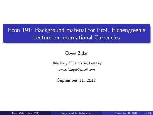
<strong>Econ</strong> <strong>191</strong>: Background material for Pr<strong>of</strong>. Eichengreen’s<br />
Lecture on International Currencies<br />
Owen Zidar<br />
<strong>University</strong> <strong>of</strong> <strong>California</strong>, <strong>Berkeley</strong><br />
owenzidargsi@gmail.com<br />
September 11, 2012<br />
Owen Zidar (<strong>Econ</strong> <strong>191</strong>) Background for Eichengreen September 11, 2012 1 / 33
Announcements<br />
Twitter: Follow @economics<strong>191</strong><br />
Sample Question: Turn in sample research question now please<br />
Attendance: Please sign attendance sheet that is going around<br />
Office Hours: Sign up online - need to see GSI once by Oct 2.<br />
Next Week: Pr<strong>of</strong>essor Eichengreen lecturing on international<br />
currencies<br />
Owen Zidar (<strong>Econ</strong> <strong>191</strong>) Background for Eichengreen September 11, 2012 2 / 33
Overview <strong>of</strong> Today’s Lecture<br />
1 Historical Context: Brief History <strong>of</strong> the Evolution <strong>of</strong> the<br />
International Monetary System<br />
2 Tools: Referesher on Multivariate Regression<br />
Owen Zidar (<strong>Econ</strong> <strong>191</strong>) Background for Eichengreen September 11, 2012 3 / 33
1. Big Picture - History <strong>of</strong> International Monetary System 1<br />
Gold Standard 1821-<strong>191</strong>4<br />
Interwar period<br />
Bretton Woods Fixed Exchange Rates: 1946-1973<br />
After Bretton Woods<br />
1 Sources: ritholtz.com/blog/ for exchange rate images and International<br />
<strong>Econ</strong>omics by Krugman and Obstfeld<br />
Owen Zidar (<strong>Econ</strong> <strong>191</strong>) Background for Eichengreen September 11, 2012 4 / 33
I. Gold Standard: 1821-<strong>191</strong>4<br />
Owen Zidar (<strong>Econ</strong> <strong>191</strong>) Background for Eichengreen September 11, 2012 5 / 33
I. Gold Standard<br />
You can “cash in” your paper notes for predetermined amount <strong>of</strong> gold<br />
Some Issues:<br />
Limits monetary growth to gold stock, which can’t be adjusted in<br />
response to economic conditions<br />
Global shortage <strong>of</strong> gold put downward pressure on prices<br />
E.g. In 1896, the U.S. price level was roughly 40% below its 1869 level<br />
Farmers were squeezed between declining prices for crops and the<br />
fixed dollar payments for their mortgages and other debts.<br />
William Jennings Bryan, Cross <strong>of</strong> Gold, and Wizard <strong>of</strong> Oz<br />
Owen Zidar (<strong>Econ</strong> <strong>191</strong>) Background for Eichengreen September 11, 2012 6 / 33
II. WWI ‘Dirty Float’ <strong>191</strong>5-1925<br />
Owen Zidar (<strong>Econ</strong> <strong>191</strong>) Background for Eichengreen September 11, 2012 7 / 33
II. Interwar Period<br />
War is Expensive: Many countries suspended gold standard, US did<br />
a few year later when it entered WWI<br />
Inflation Taxes<br />
Strength in US: US returned to Gold in <strong>191</strong>9<br />
Genoa: 1922 conference establishing gold exchange standard 2<br />
Restricted Monetary Flexibility: 1925 Britain returned to the gold<br />
standard. Contractionary policy to get back to prewar price level.<br />
2 Countries could hold securities convertible into gold issued by other<br />
countries as reserves<br />
Owen Zidar (<strong>Econ</strong> <strong>191</strong>) Background for Eichengreen September 11, 2012 8 / 33
II. Interwar Gold-Exchange Standard: 1926-1931<br />
Owen Zidar (<strong>Econ</strong> <strong>191</strong>) Background for Eichengreen September 11, 2012 9 / 33
II. Pre-Bretton Woods Floats: 1932-1944<br />
Owen Zidar (<strong>Econ</strong> <strong>191</strong>) Background for Eichengreen September 11, 2012 10 / 33
III. Bretton Woods: 1945-1971<br />
Fixed exchange rates against the dollar<br />
Unvarying dollar price <strong>of</strong> gold: $35 an ounce<br />
Member countries held international reserves in dollars<br />
They had the right to sell dollars for gold at the <strong>of</strong>ficial price 3<br />
They also had the right to adjust their peg to the dollar (pending IMF<br />
agreement)<br />
3 Bretton Woods differed from interwar gold exchange standard in that the<br />
right to sell dollars to the Treasury for gold was limited to <strong>of</strong>ficial foreign<br />
creditors (governments and central banks<br />
Owen Zidar (<strong>Econ</strong> <strong>191</strong>) Background for Eichengreen September 11, 2012 11 / 33
III. Bretton Woods: 1945-1971<br />
Owen Zidar (<strong>Econ</strong> <strong>191</strong>) Background for Eichengreen September 11, 2012 12 / 33
IV. Smithsonian Agreement: 1972-1973<br />
Owen Zidar (<strong>Econ</strong> <strong>191</strong>) Background for Eichengreen September 11, 2012 13 / 33
III. Floats and Pegs: 1974-1979<br />
US macro policies in the late 1960s helped cause the breakdown <strong>of</strong><br />
Bretton Woods by early 1973<br />
Most advanced countries abandoned stated pegs, while many<br />
developing countries stayed pegged<br />
1974-1975: Stagflation 4 led most gov’ts to use monetary and fiscal<br />
policy<br />
Many attempts to coordinate pseudo-fixed exchange rates within<br />
Europe<br />
4 Stagnant growth, high inflation. Higher commodity prices increased<br />
inflation & depressed output. Expectations <strong>of</strong> future inflation fed into wages &<br />
prices<br />
Owen Zidar (<strong>Econ</strong> <strong>191</strong>) Background for Eichengreen September 11, 2012 14 / 33
IV. Floats and Pegs: 1974-1979<br />
Owen Zidar (<strong>Econ</strong> <strong>191</strong>) Background for Eichengreen September 11, 2012 15 / 33
IV. ERM, Euro, ... : 1980-<br />
Dollar Fluctuates: 1976-1979 Weak Dollar, Paul Volker & Deficits,<br />
Joint Intervention to depreciate in 1985<br />
ERM semi-pegged system: member banks would intervene to<br />
maintain 2.25% band. UK joined in 1990 and exited 2 years after.<br />
German Reunification: 1990 reunification set <strong>of</strong>f inflationary<br />
pressures, divergent needs in Europe and speculative attacks (leading<br />
to 15% bands in 1993).<br />
Inflation Convergence: European countries peg to deutche mark<br />
within Europe’s fixed exchange rate mechanism EMS 5<br />
Euro: Maastrict Treaty and a common currency in 1999<br />
Asian Crisis <strong>of</strong> 1997: Many stopped adhering to dollar pegs after<br />
5 European Monetary System<br />
Owen Zidar (<strong>Econ</strong> <strong>191</strong>) Background for Eichengreen September 11, 2012 16 / 33
IV. ERM, Euro, ... : 1980-<br />
Owen Zidar (<strong>Econ</strong> <strong>191</strong>) Background for Eichengreen September 11, 2012 17 / 33
Part 2: Multivariate Regression Refresher 6<br />
Contents<br />
1 Preliminaries<br />
2 Big picture idea: summarize data<br />
3 Linear model<br />
4 Multivariate<br />
Frisch Waugh interpretation<br />
Omitted Variable Bias<br />
Reading reg output<br />
5 Methods: D-D and IV<br />
6 Probit<br />
6 Some <strong>of</strong> these notes are based on Mostly Harmless <strong>Econ</strong>ometrics and<br />
Charlie Gibbon’s 140 notes<br />
Owen Zidar (<strong>Econ</strong> <strong>191</strong>) Background for Eichengreen September 11, 2012 18 / 33
1. Preliminaries<br />
1 Expectations<br />
2 Variance<br />
3 Covariance<br />
E(Y ) = Y1 × Prob1 + Y2 × Prob2 + ... + Yj × Probj<br />
Var(Y ) = E[Y − µy ] 2<br />
(1)<br />
(2)<br />
Cov(X , Y ) = E[X − µx][Y − µy ] (3)<br />
Owen Zidar (<strong>Econ</strong> <strong>191</strong>) Background for Eichengreen September 11, 2012 19 / 33
2. Big picture<br />
Owen Zidar (<strong>Econ</strong> <strong>191</strong>) Background for Eichengreen September 11, 2012 20 / 33
3. Linear model<br />
Decomposition<br />
Example: Height by gender<br />
yi = E[yi|xi] + (yi − E[yi|xi])<br />
� �� �<br />
≡ɛi<br />
= β0 + β1xi + ɛi<br />
Owen Zidar (<strong>Econ</strong> <strong>191</strong>) Background for Eichengreen September 11, 2012 21 / 33<br />
(4)<br />
(5)
3. Linear model Continued<br />
What is β1? β1 = Cov(x,y)<br />
Var(x)<br />
Owen Zidar (<strong>Econ</strong> <strong>191</strong>) Background for Eichengreen September 11, 2012 22 / 33
4. Multivariate model<br />
(6)<br />
yi = β0 + β1x1i + β2x2i + ... + +βkxki + ɛi<br />
βk =<br />
Cov(y, ˜xk)<br />
Var( ˜xk)<br />
where ˜xk is the residual regression <strong>of</strong> xk on all the other covariates.<br />
Takeaway: βk is the relationship between y and the part <strong>of</strong> xk that<br />
isn’t related to other x’s<br />
Owen Zidar (<strong>Econ</strong> <strong>191</strong>) Background for Eichengreen September 11, 2012 23 / 33<br />
(7)
4. Multivariate model: Omitted Variable Bias<br />
Suppose that the true model is<br />
yi = γ0 + γ1Schoolingi + γ2Abilityi + ˜ɛi<br />
Also suppose that Abilityi can be written:<br />
Abilityi = α0 + α1Schoolingi + ηi<br />
What happens if we omit ability and run a “short” regression?<br />
yi = β0 + β1Schoolingi + ɛi<br />
(8)<br />
(9)<br />
(10)<br />
Owen Zidar (<strong>Econ</strong> <strong>191</strong>) Background for Eichengreen September 11, 2012 24 / 33
4. Multivariate model: Omitted Variable Bias cont.<br />
What happens if we omit ability and run a “short” regression?<br />
Plug in ability expression from (10) into true model to see<br />
Takeaways<br />
yi = γ0 + γ1Schoolingi + γ2(α0 + α1Schoolingi + ηi) + ˜ɛi<br />
yi = (γ0 + γ2) + (γ1 + γ2α1) Schoolingi + (ηi + ˜ɛi)<br />
� �� � � �� �<br />
� �� �<br />
ɛi<br />
β1<br />
β2<br />
β2 = γ1 + γ2α1<br />
Short equals long plus the effect <strong>of</strong> omitted times the regression <strong>of</strong><br />
omitted on included.<br />
Does γ2α1 = 0?<br />
Owen Zidar (<strong>Econ</strong> <strong>191</strong>) Background for Eichengreen September 11, 2012 25 / 33
4. Reading regression output<br />
Owen Zidar (<strong>Econ</strong> <strong>191</strong>) Background for Eichengreen September 11, 2012 26 / 33
5. Methods: Difference in Difference<br />
Effect = [After-Before]Treatment − [After − Before]Control<br />
Owen Zidar (<strong>Econ</strong> <strong>191</strong>) Background for Eichengreen September 11, 2012 27 / 33
5. Methods: Instrumental Variables<br />
Setup<br />
yi = γ0 + γ1Schoolingi + γ2Abilityi + ˜ɛi<br />
� �� �<br />
≡vi<br />
Exclusion Restriction: 7 An instrument, zi, is correlated with Schoolingi<br />
but uncorrelated with other determinants <strong>of</strong> dependent variables<br />
Cov(vi, zi) = 0<br />
Cov(yi − γ0 − γ1Schooling,zi) = 0<br />
Cov(yi, zi) − γ1Cov(Schooling,zi) = 0<br />
Cov(yi, zi)<br />
= γ1<br />
Cov(Schooling,zi)<br />
7 because zi can be “excluded” from the causal model<br />
(11)<br />
Owen Zidar (<strong>Econ</strong> <strong>191</strong>) Background for Eichengreen September 11, 2012 28 / 33
5. Methods: Instrumental Variables continued<br />
Implementing this: First stage and reduced form<br />
γ1 =<br />
γ1 =<br />
Schoolingi = θ0 + θ1zi + ηi<br />
γ1 = π1<br />
θ1<br />
yi = π0 + π1zi + ui<br />
Cov(yi, zi)<br />
Cov(Schooling,zi)<br />
Cov(yi, zi)/Var(zi)<br />
Cov(Schooling,zi)/Var(zi)<br />
Caution: Important that first stage is strong (rule <strong>of</strong> thumb is F > 10)<br />
(12)<br />
(13)<br />
Owen Zidar (<strong>Econ</strong> <strong>191</strong>) Background for Eichengreen September 11, 2012 29 / 33
6. Probit 8<br />
What if limited dependent variable? Yi = 0 or Yi = 1<br />
8 Graph from Ashenfelter et al’s Statistics and <strong>Econ</strong>ometrics Book<br />
Owen Zidar (<strong>Econ</strong> <strong>191</strong>) Background for Eichengreen September 11, 2012 30 / 33
6. Probit (continued)<br />
Setup:<br />
Marginal Effects:<br />
E(Yi) = Pr(Yi = 0)0 +Pr(Yi = 1)1<br />
� �� �<br />
=0<br />
= Pr(Yi = 1)<br />
≡ Φ(xiβ)<br />
� �� �<br />
probit<br />
∂Pi<br />
∂xi<br />
= ∂Φ(xiβ)<br />
∂xi<br />
= βφ(xiβ)<br />
where Φ is the c.d.f. and φ is the p.d.f. <strong>of</strong> the normal distribution 9<br />
9 Φ is prob(z < xiβ), z ∼ N(0, 1), so need to standardize if actually using this<br />
Owen Zidar (<strong>Econ</strong> <strong>191</strong>) Background for Eichengreen September 11, 2012 31 / 33
6. Probit continued<br />
What does this look like in a graph?<br />
Owen Zidar (<strong>Econ</strong> <strong>191</strong>) Background for Eichengreen September 11, 2012 32 / 33
Next Time<br />
Pr<strong>of</strong>essor Eichengreen on International Currencies<br />
Owen Zidar (<strong>Econ</strong> <strong>191</strong>) Background for Eichengreen September 11, 2012 33 / 33


