EMS Newsletter June 2010 - European Mathematical Society ...

Feature
Most evolution is neutral
In 1968, Kimura surprised the scientific community with the
idea that most genome mutations are neutral [12]. His argument
goes as follows. Comparative studies of some proteins
lead to the conclusion that chains 100 amino acids long undergo
one substitution every 28 million years. The length of
DNA chains in the two chromosome sets of mammals is about
4 × 10 9 base pairs. Every three base pairs code for one amino
acid and, due to the existing redundancy, only 80 % of base
pair substitutions lead to an amino acid substitution. Therefore
there are 16 million substitutions in the whole genome
every 28 million years, i.e. almost one substitution every 2
years! Kimura’s conclusion is that organisms can only afford
such a mutational load provided the great majority of mutations
are neutral.
Recent studies on RNA molecules reach similar conclusions
[6]. RNA molecules fold as a result of the interaction
between the bases forming their sequences. This folding can
be regarded as the molecule phenotype because it determines
the function of these chains. Thus natural selection acts directly
on it being blind to the actual sequences. The number
of different sequences folding into the same structure is huge.
This implies, once more, that a large number of mutations
in the chain leave the phenotype intact, thus avoiding selection.
Neutrality seems the rule rather than the exception, at least
at the molecular level. The consequences of this fact are far
reaching but to see how much, we need to introduce a new
concept: adaptive landscapes, and resort again to mathematics.
6 Adaptive landscapes
Perhaps Sewall Wright’s most relevant contribution to evolutionary
theory is his metaphor of adaptive landscape [19].
From a formal viewpoint, an adaptive landscape is a mapping
f : X→R, where X denotes a configuration space equipped
with some notion of adjacency, proximity, distance or accessibility,
and whose image is the fitness associated to a particular
configuration in X. This structure, together with the fact
that the set of all adaptive landscapes forms the vector space
R |X| , allows the development of a rich theory of combinatorial
landscapes that covers not only the adaptive landscapes
of biology but also the energy landscapes of physics or the
combinatorial optimization problems arising in computer science
[17].
abcd
Abcd
aBcd
abCd
abcD
ABcd
AbCd
AbcD
aBCd
aBcD
abCD
ABCd
ABcD
AbCD
aBCD
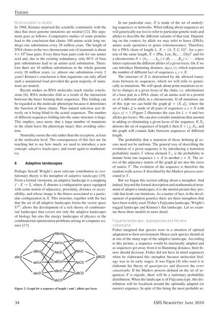
Figure 2. Graph for a sequence of length 4 and 2 alleles per locus
ABCD
In our particular case, X is made of the set of underlying
sequences or networks. When talking about sequences we
will generically use loci to refer to particular genetic traits and
alleles to describe the different variants of that trait. Depending
on the context, by allele we may refer to bases (DNA),
amino acids (proteins) or genes (chromosomes). Therefore,
for a DNA chain of length L, X = {A, T, C, G} L , for a pro-
tein of the same length, X = {Phe, Leu, Ile,. . . , Gly} L and for
a chromosome X = {A1,...,Ana }×{B1,...,Bnb }×···, where
letters represent the different alleles of a given locus. On X we
can introduce Hamming distance, dH(x, y), which represents
the number of different loci of sequences x, y ∈X.
The structure of X is determined by the allowed transitions
between its sequences, which we will refer to generically
as mutations. We will speak about point mutations to refer
to changes at a given locus of the chain, i.e. substitutions
of a base pair in a DNA chain, of an amino acid in a protein
or of a different allele in a chromosome. If all mutations are
of this type we can build the graph G = {X, L}, where the
set of links L is made of all pairs of sequences x, y ∈Xwith
dH(x, y) = 1 (Figure 2 illustrates the case for L = 4 and two
alleles per locus). We can also consider mutations that amount
to adding or eliminating a given locus of the sequence. If XL
denotes the set of sequences of length L then X = � L XL, and
the graph will contain links between sequences of different
length.
The probability that a mutation of those defining G occurs
need not be uniform. The general way of describing the
evolution of a given sequence is by introducing a transition
probability matrix T whose element Txy is the probability to
mutate from one sequence x ∈Xto another y ∈X. The zeros
of the adjacency matrix of the graph G are also the zeros
of matrix T. The evolution of the sequence is therefore the
random walk across X described by the Markov process associated
to T.
But we began this section talking about a metaphor. And
indeed, beyond the formal description and mathematical treatment
of adaptive landscapes, it is the mental picture they provide
that leads our intuitions. As a matter of fact, in the development
of population genetics there are three metaphors that
have been widely used: Fisher’s Fujiyama landscape, Wright’s
rugged landscape and Kimura’s flat landscape. Let us examine
these three models in more detail.
Fujiyama landscape: quasispecies and the error
catastrophe
Fisher imagined that species were in a situation of optimal
adaptation to their environment. Hence each species should sit
at one of the many tops of the adaptive landscape. According
to this picture, a sequence would be maximally adapted and
as sequences get away from it in Hamming distance, their fitness
should decrease. Fisher did not have in mind sequences
when he elaborated this metaphor because molecular biology
was in its early stages. It was Eigen [4] who used it to
elaborate his theory of quasispecies and discover the error
catastrophe. If the Markov process defined on the set of sequences
X is ergodic, there will be a stationary probability
distribution. When the landscape is of Fujiyama type, this distribution
will be localized around the optimally adapted (or
master) sequence. In spite of this being the most probable se-
34 EMS Newsletter June 2010