EMS Newsletter June 2010 - European Mathematical Society ...

quence, close to it (i.e. a few mutations away) there will be a
“cloud” of less adapted sequences coexisting with the master
sequence. Quasispecies is the term that Eigen introduced to
describe this ensemble of sequences.
In order to study the behaviour of a quasispecies more
closely we will resort to equation (9). For simplicity we shall
assume that sequences have finite length L � 1, that there
are just two alleles per locus, that the master sequence has
fitness f1 = f > 1 and that all other sequences have fitness
f2 = ··· = f 2 L = 1. We shall also assume that the probability
that a point mutation occurs is μ � 1, independent of the
sequence. Let x1 = x denote the population fraction of the
master sequence; thus x2 +···+ x 2 L = 1− x and φ = fx+1− x.
Equation (9) then becomes
˙x = x � f (1 − μ) L − 1 − ( f − 1)x � + O(μ). (34)
The term O(μ) accounts for the transitions from the L nearest
neighbour sequences of the master sequence that revert
to the master sequence. Neglecting these terms and approximating
(1 − μ) L ≈ e −Lμ we can see that if fe −Lμ > 1 then x
asymptotically approaches x ∗ = (e −Lμ f − 1)/( f − 1), whereas
if fe −Lμ < 1 the bracket in equation (34) becomes negative
and therefore x = O(μ). The threshold μerr = log f /L defines
the error catastrophe. When μμerr the identity of this master sequence
gets lost in the cloud of mutants and the quasispecies disappears
as such.
Experimental studies performed in the ’90s seem to confirm
[16] that indeed the length of the genome of different
species – ranging from virus to Homo sapiens – and the mutation
rate per base are related as μL ≤ O(1). Hence an increase
in the mutation rate is a mechanism that this theory puts forward
to fight viral infections. We will come back to this point
later.
Rugged landscape
Although locally the adaptive landscape can be well described
by the Fujiyama model, Wright visualized it as a rugged landscape,
full of high peaks separated by deep valleys. The reason
is that mutations that change the sequence minimally may
induce large variations in the fitness of individuals. In addition,
there exists the well known phenomenon of epistasis,
according to which some genes interact, either constructively
or destructively, amplifying these large variations in response
to small changes in the sequences.
According to the rugged landscape metaphor, species evolve
by climbing peaks and sitting on the summits. Different peaks
correspond to different species with different fitnesses. This
picture seems to fit well with our idea of evolution by natural
selection. However, it has a serious drawback: species
that are at a summit can only move to a higher one by going
through an unfit valley. In the most favourable case this valley
will consist of a single intermediate state. Formula (31) tells
us that if a population is small, it is not impossible that an
unfit allele replaces a fitter one. Nevertheless, the probability
that this happens is very small, i.e. adaptation times should
be very large. And this is only the most favourable case. The
high speed of adaptation to rapidly changing environments
Feature
that viruses exhibit seriously challenges this model. What is
then wrong in our picture of adaptive landscapes?
Holey landscape: neutral networks
Let us review the most extreme case of a rugged landscape:
the random landscape. In this case every sequence of X has a
random fitness, independent of the other sequences. In general,
rugged landscapes are not that extreme because there
is some degree of correlation between the fitness of neighbouring
sequences. However, beyond the correlation length,
fitness values become uncorrelated. The random landscape is
the extreme case in which the correlation length is smaller
than 1. Suppose now that the length of the sequences is large,
and that every locus can host A independent alleles. The degree
of graph G will thus be g = (A−1)L and its size |X| = AL .
With L = 100 and A = 2 (a rather modest choice), g = 100
and |X| = 2100 ≈ 1030 . To all purposes such a graph can be
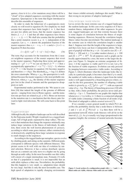
locally approximated by a tree, the more so the larger the degree
(see Figure 3). Imagine an extreme assignment of fitness:
1 if the sequence is viable and 0 if it is not. Let p be
the fraction of viable sequences. Evolution can only proceed
by jumping between consecutive viable nodes. According to
Figure 3, which illustrates what this landscape looks like locally
in a particular graph, it becomes clear that if p is small,
the number of viable nodes a distance d apart from the initial
node is well approximated by a branching process where, except
for the first generation, the number of offspring (viable
nodes) is given by pk = � �
g−1 k g−1−k
k p (1 − p) , with an expected
value of (g −1)p. The theory of branching processes [10] tells
us that, with a finite probability, the process never ends provided
(g − 1)p > 1. Translated to our graphs this implies that
whenever p � 1/g (with g � 1) there is a connected subgraph
of viable nodes containing a finite fraction of all nodes of G.
This kind of subgraph is called a neutral network [7].
If we consider a more general model in which P( f ) describes
the probability density that a node fitness is between
f and f + df, if � f2
P( f ) df � 1/g then there will be a
f1
quasineutral network whose node fitnesses will all lie in the
interval ( f1, f2). As g is usually very large (proportional to the
sequence length), the existence of neutral networks becomes
Figure 3. Local section of a configuration graph with A = 2 and L = 8.
Black nodes are viable, whereas white nodes are not viable.
EMS Newsletter June 2010 35