Modern Empirical Cost and Schedule Estimation Tools
Modern Empirical Cost and Schedule Estimation Tools
Modern Empirical Cost and Schedule Estimation Tools

Create successful ePaper yourself
Turn your PDF publications into a flip-book with our unique Google optimized e-Paper software.
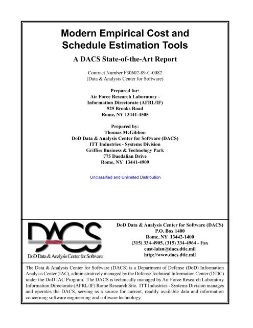
<strong>Modern</strong> <strong>Empirical</strong> <strong>Cost</strong> <strong>and</strong><br />
<strong>Schedule</strong> <strong>Estimation</strong> <strong>Tools</strong><br />
A DACS State-of-the-Art Report<br />
Contract Number F30602-89-C-0082<br />
(Data & Analysis Center for Software)<br />
Prepared for:<br />
Air Force Research Laboratory -<br />
Information Directorate (AFRL/IF)<br />
525 Brooks Road<br />
Rome, NY 13441-4505<br />
Prepared by:<br />
Thomas McGibbon<br />
DoD Data & Analysis Center for Software (DACS)<br />
ITT Industries - Systems Division<br />
Griffiss Business & Technology Park<br />
775 Daedalian Drive<br />
Rome, NY 13441-4909<br />
DoD Data & Analysis Center for Software (DACS)<br />
P.O. Box 1400<br />
Rome, NY 13442-1400<br />
(315) 334-4905, (315) 334-4964 - Fax<br />
cust-laisn@dacs.dtic.mil<br />
http://www.dacs.dtic.mil<br />
The Data & Analysis Center for Software (DACS) is a Department of Defense (DoD) Information<br />
Analysis Center (IAC), administratively managed by the Defense Technical Information Center (DTIC)<br />
under the DoD IAC Program. The DACS is technically managed by Air Force Research Laboratory<br />
Information Directorate (AFRL/IF) Rome Research Site. ITT Industries - Systems Division manages<br />
<strong>and</strong> operates the DACS, serving as a source for current, readily available data <strong>and</strong> information<br />
concerning software engineering <strong>and</strong> software technology.
REPORT DOCUMENTATION PAGE<br />
Form Approved<br />
OMB No. 0704-0188<br />
Public reporting burden for this collection is estimated to average 1 hour per response including the time for reviewing instructions, searching existing data sources, gathering <strong>and</strong> maintaining the<br />
data needed <strong>and</strong> completing <strong>and</strong> reviewing the collection of information. Send comments regarding this burden estimate or any other aspect of this collection of information, including suggestions<br />
for reducing this burden to Washington Headquarters Services, Directorate for Information Operations <strong>and</strong> Reports. 1215 Jefferson Davis Highway, Suite 1204, Arlington, VA 22202-4302, <strong>and</strong> to<br />
the Office of Management <strong>and</strong> Budget, Paperwork Reduction Project, (0704-0188). Washington, DC 20503.<br />
1. AGENCY USE ONLY (Leave Blank) 2. REPORT DATE 3. REPORT TYPE AND DATES COVERED<br />
4. TITLE AND SUBTITLE 5. FUNDING NUMBERS<br />
A State-of-the-Art-Report<br />
<strong>Modern</strong> <strong>Empirical</strong> <strong>Cost</strong> <strong>and</strong> <strong>Schedule</strong> <strong>Estimation</strong> <strong>Tools</strong><br />
F30602-89-C-0082<br />
6. AUTHORS<br />
Thomas McGibbon - DACS<br />
7. PERFORMING ORGANIZATIONS NAME(S) AND ADDRESS(ES) 8. PERFORMING ORGANIZATION<br />
REPORT NUMBER<br />
ITT Industries, Systems Division, 775 Daedalian Drive DACS-SOAR-97-1<br />
Rome, NY 13441-4909<br />
11. SUPPLEMENTARY NOTES<br />
Available from: DoD Data & Analysis Center for Software (DACS)<br />
775 Daedalian Drive, Rome, NY 13441-4909<br />
12a. DISTRIBUTION/ AVAILABILITY STATEMENT 12b. DISTRIBUTION CODE<br />
13. ABSTRACT (Maximum 200 words)<br />
20 August 1997 N/A<br />
9. SPONSORING/MONITORING AGENCY NAME(S) AND ADDRESS(ES) 10. SPONSORING/MONITORING<br />
Defense Technical Information Center (DTIC)/ AI<br />
AGENCY REPORT NUMBER<br />
8725 John J. Kingman Rd., STE 0944, Ft. Belvoir, VA 22060<br />
<strong>and</strong> Air Force Research Lab/IFTD N/A<br />
525 Brooks Rd., Rome, NY 13440<br />
Approved for public release, distribution unlimited UL<br />
<strong>Cost</strong> models were derived from the collection <strong>and</strong> analysis of large collections of project data. Modelers<br />
would fit a curve to the data <strong>and</strong> analyze those parameters that affected the curve. Early models applied to<br />
custom-developed software systems. New software development philosophies <strong>and</strong> technologies have<br />
emerged in the 1980s <strong>and</strong> 1990s to reduce development costs <strong>and</strong> improve quality of software products.<br />
These new approaches frequently involve the use of Commercial-Off-The-Shelf (COTS) software,<br />
software reuse, application generators, <strong>and</strong> fourth generation languages. The purpose of this paper is to<br />
identify, discuss, compare <strong>and</strong> contrast software cost estimating models <strong>and</strong> tools that address these<br />
modern philosophies<br />
14. SUBJECT TERMS<br />
<strong>Empirical</strong> Data, Datasets, <strong>Cost</strong> <strong>Estimation</strong>, Software <strong>Tools</strong>,<br />
15. NUMBER OF PAGES<br />
21<br />
Metrics Software Measurement<br />
16. PRICE CODE<br />
N/A<br />
17. SECURITY CLASSIFICATION 18. SECURITY CLASSIFICATION 19. SECURITY CLASSIFICATION 20. LIMITATION OF<br />
OF REPORT OF THIS PAGE OF ABSTRACT ABSTRACT<br />
Unclassified Unclassified Unclassified UL<br />
NSN 7540-901-280-5500 St<strong>and</strong>ard Form 298 (Rev 2-89)
<strong>Modern</strong> <strong>Modern</strong> <strong>Empirical</strong> <strong>Empirical</strong> <strong>Cost</strong> <strong>Cost</strong> <strong>and</strong><br />
<strong>and</strong><br />
<strong>Schedule</strong> <strong>Schedule</strong> <strong>Estimation</strong> <strong>Estimation</strong> <strong>Tools</strong><br />
<strong>Tools</strong><br />
Table of Contents<br />
Abstract & Ordering Information ____________________________________ 1<br />
1. Executive Summary ____________________________________ 2<br />
2. World Wide Web Resources _____________________________ 3<br />
• Cocomo............................................................................ 3<br />
• Function Points ................................................................ 3<br />
• Software <strong>Cost</strong> Estimating <strong>Tools</strong> ...................................... 4<br />
3. Comparison of Products ________________________________ 5<br />
a. Cocomo 1.1 ...................................................................... 9<br />
b. Cocomo 2.0 .................................................................... 10<br />
c. Putnam Software Equation ............................................ 13<br />
d. PRICE-S ........................................................................ 15<br />
e. Function Point <strong>Cost</strong> <strong>Estimation</strong> ..................................... 16<br />
f. Other Models .................................................................. 16<br />
Appendix A: Bibliography ________________________________________ 17<br />
Tables Referenced in Document<br />
Table 1: Effort Equations .................................................................................................... 6<br />
Table 2: <strong>Schedule</strong> Equations............................................................................................... 9<br />
Table 3: UFP to SLOC Conversion Table ........................................................................ 11<br />
Table 4: Putnam Productivity Parameter .......................................................................... 14<br />
Table 5: Putnam Special Skills Factor .............................................................................. 15<br />
Figures Referenced in Document<br />
Figure 1: Comparison of COCOMO Effort Equations....................................................... 7<br />
Figure 2: Comparison of Effort Equations ......................................................................... 8<br />
<strong>Modern</strong> <strong>Empirical</strong> <strong>Cost</strong> <strong>and</strong> <strong>Schedule</strong> <strong>Estimation</strong> <strong>Tools</strong>
Acknowledgements:<br />
<strong>Modern</strong> <strong>Modern</strong> <strong>Empirical</strong> <strong>Empirical</strong> <strong>Cost</strong> <strong>Cost</strong> <strong>and</strong><br />
<strong>and</strong><br />
<strong>Schedule</strong> <strong>Schedule</strong> <strong>Estimation</strong> <strong>Estimation</strong> <strong>Tools</strong><br />
<strong>Tools</strong><br />
Abstract <strong>and</strong> Ordering Information<br />
Abstract<br />
<strong>Cost</strong> models were derived from the collection <strong>and</strong> analysis of large collections of project data. Modelers<br />
would fit a curve to the data <strong>and</strong> analyze those parameters that affected the curve. Early models applied to<br />
custom-developed software systems. New software development philosophies <strong>and</strong> technologies have<br />
emerged in the 1980s <strong>and</strong> 1990s to reduce development costs <strong>and</strong> improve quality of software products.<br />
These new approaches frequently involve the use of Commercial-Off-The-Shelf (COTS) software,<br />
software reuse, application generators, <strong>and</strong> fourth generation languages. The purpose of this paper is to<br />
identify, discuss, compare <strong>and</strong> contrast software cost estimating models <strong>and</strong> tools that address these<br />
modern philosophies.<br />
Ordering Information:<br />
A bound version of this report, is avaliable for $30 from the DACS Product Orderform or you may order<br />
it by contacting:<br />
DACS Customer Liaison<br />
775 Dadaelian Drive<br />
Griffiss Business Park<br />
Rome, NY 13441-4909<br />
(315) 334-4905; Fax: (315) 334-4964;<br />
cust-liasn@dacs.dtic.mil<br />
The author would like to gratefully acknowledge comments on an earlier draft by Mr. Robert Vienneau<br />
<strong>and</strong> the help of Mr. Lon R. Dean in producing this report.<br />
A DACS State-of-the Art-Report<br />
1
1. Executive Summary<br />
Project managers <strong>and</strong> project planners are often expected to provide to their management estimates of<br />
schedule length <strong>and</strong> costs for upcoming projects or products. Anyone that has tried to construct <strong>and</strong> justify<br />
such an estimate for a software development project of any size knows that it can be an art to achieve<br />
reasonable levels of accuracy <strong>and</strong> consistency. <strong>Empirical</strong>ly-based cost estimation models supporting<br />
management needs began to appear in the literature during the 1970s <strong>and</strong> 1980s. Support services for<br />
some of these models also became commercially available.<br />
<strong>Cost</strong> models were derived from the collection <strong>and</strong> analysis of large collections of project data. Modelers<br />
would fit a curve to the data <strong>and</strong> analyze those parameters that affected the curve. Early models applied to<br />
custom-developed software systems. New software development philosophies <strong>and</strong> technologies have<br />
emerged in the 1980s <strong>and</strong> 1990s to reduce development costs <strong>and</strong> improve quality of software products.<br />
These new approaches frequently involve the use of Commercial-Off-The-Shelf (COTS) software,<br />
software reuse, application generators, <strong>and</strong> fourth generation languages. The purpose of this paper is to<br />
identify, discuss, compare <strong>and</strong> contrast software cost estimating models <strong>and</strong> tools that address these<br />
modern philosophies.<br />
In evaluating <strong>and</strong> selecting an estimation tool, or estimation tool provider, one should evaluate:<br />
• The openness of the underlying model in the tool<br />
• The platform requirements of the tool<br />
• The data required as input to the tool<br />
• The output of the tool<br />
• The accuracy of the estimates provided by the model<br />
The openness of the tool developer in providing details of the underlying model <strong>and</strong> parameters is one<br />
attribute distinguishing some models from others. Volumes of information have been published about the<br />
models underlying some tools. The vendors of other tools keep information about their model as<br />
proprietary <strong>and</strong> require the user to purchase consulting services to exercise the model. This may not be a<br />
practical problem since beginners will most likely hire consulting services anyways, especially if they are<br />
not a statistician or modeler. But, since many of the models can be implemented with a simple<br />
spreadsheet, being able to underst<strong>and</strong> the “guts” of the model may be important so as to allow one to<br />
enhance the model to meet specific needs.<br />
Several cost models have been implemented in commercial toolsets. Those considering purchasing these<br />
products need to consider the platform on which the product is implemented. Most commercial cost<br />
modeling tools are only available on Windows-based platforms. You will have to determine if your<br />
hardware meets minimal requirements for the toolset.<br />
Major factors in selecting a model include assessing the number <strong>and</strong> complexity of required input<br />
parameters, whether default values can be easily <strong>and</strong> underst<strong>and</strong>ably assigned to these parameters, <strong>and</strong><br />
whether sufficient historical <strong>and</strong> project data exists within one’s organization <strong>and</strong> project to feed the<br />
model. Many of the models are very flexible in modeling specific situations. To achieve this flexibility,<br />
model providers provide numerous parameters to h<strong>and</strong>le multiple situations. A substantial amount of time<br />
may be required to initially set-up a model - one must either answer a number of questions or collect<br />
significant amounts of historical data on similar projects. If an established measurement program exists<br />
within an organization, assembling the required data may not be too difficult. Most models provide ways<br />
<strong>Modern</strong> <strong>Empirical</strong> <strong>Cost</strong> <strong>and</strong> <strong>Schedule</strong> <strong>Estimation</strong> <strong>Tools</strong><br />
2
to refine estimates as one gains experience with the model. One beneficial side-effect of cost models is<br />
that they identify measures to collect <strong>and</strong> manage in an organization.<br />
Evaluate the outputs <strong>and</strong> reports from the model. All software cost models estimate project costs, effort,<br />
<strong>and</strong> nominal schedule for a project. Determine whether other data not estimated by the model (such as<br />
travel expenses, overhead costs, etc.) can be easily integrated into the reports being generated. Some<br />
models provide additional management guidance in their reporting structure. For example, some models<br />
provide staffing profile guidance <strong>and</strong> determine optimum staff size for a project.<br />
Perhaps the most important feature of any model is the accuracy of the estimate provided. One should try to<br />
collect as much data as possible from completed software projects. One can determine with this data whether<br />
a model would have accurately estimated those projects <strong>and</strong> how to fine-tune the model for a given<br />
environment. If a model gives wildly inacurate or inconsistent results, one should consider other models.<br />
2. World Wide Web Resources<br />
* The Constructive <strong>Cost</strong> Model (COCOMO) is a well-known model used in software cost <strong>and</strong> schedule<br />
estimation. It is a non-proprietary model introduced by Barry W. Boehm in 1981.<br />
COCOMO Project Homepage <br />
The COCOMO 2.0 model is an update of COCOMO 1981 to address software development practices<br />
in the 1990s <strong>and</strong> 2000s. It is being developed by USC-CSE, UC Irvine, <strong>and</strong> 29 affiliate organizations.<br />
REVIC Software <strong>Estimation</strong> Model <br />
Includes a downloadable version of Revised Intermediate COCOMO (REVIC) <strong>and</strong> pointers to more<br />
information about software cost modeling.<br />
Softstar Systems <br />
Developers of <strong>Cost</strong>ar, an automated implementation of COCOMO.<br />
* Function Points provide a unit of measure for software size using logical functional terms readily<br />
understood by business owners <strong>and</strong> users.<br />
International Function Point Users Group <br />
IFPUG is a membership-governed, non-profit organization committed to increasing the effectiveness<br />
of its members’ information technology environments through the application of Function Point<br />
Analysis (FPA) <strong>and</strong> other software measurement techniques.<br />
Function Point FAQ <br />
A comprehensive Function Points FAQ, edited by Ray Boehm of Software Composition Technologies<br />
Metre v2.3 <br />
Metre is a freely distributable ANSI/ISO St<strong>and</strong>ard C parser. Reports Halstead metrics, various line <strong>and</strong><br />
statement counts, backfired Function Points, control depth, identifier count, number of functions <strong>and</strong><br />
modules, <strong>and</strong> a call graph.<br />
A DACS State-of-the Art-Report<br />
3
Programs for C Source Code Metrics <br />
Some free programs to count lines of code, cyclomatic complexity, Halstead metrics, backfired<br />
Function Points, etc. for C code. The tools can be compiled on SunOS.<br />
* Software <strong>Cost</strong> Estimating <strong>Tools</strong><br />
<strong>Cost</strong>.Xpert <br />
<strong>Cost</strong>.Xpert, produced by Martoz, Incorporated, provides a step-by-step approach to defining a project’s<br />
cost <strong>and</strong> schedule. It is backed by years of research <strong>and</strong> comprehensive historical databases. <strong>Cost</strong>.Xpert<br />
is an easy-to-use software costing tool with the features <strong>and</strong> sophistication typical of more expensive<br />
programs. It supports all popular forms of cost estimating including COCOMO <strong>and</strong> Function Points.<br />
PRICE Systems <br />
PRICE-S is a well-known software cost estimating model. Quantitative Software Management Lawrence Putnam is the president of QSM. They distribute SLIM <strong>and</strong> related<br />
software cost modeling tools.<br />
Resource Calculations, Inc. <br />
RCI distributes sizing <strong>and</strong> cost models, including ASSET-R, SSM, <strong>and</strong><br />
SOFTCOST-R. Software Productivity Research Information Center <br />
A leading provider of software measurement, assessment, <strong>and</strong> estimation products <strong>and</strong> services. Capers<br />
Jones is SPR’s chairman <strong>and</strong> founder.<br />
* Other Web Resources<br />
NASA Johnson Space Center (JSC) <strong>Cost</strong> Estimating Group <br />
Includes a reference manual for parametric cost estimation. This group supports JSC directorates <strong>and</strong><br />
program offices with parametric cost estimates, trade studies, schedule analyses, cost-risk analyses,<br />
<strong>and</strong> cost phasing. This includes economic analyses of alternative investments, if applicable. They<br />
prepare <strong>and</strong> document cost estimates. They present <strong>and</strong> defend cost estimates to senior management<br />
<strong>and</strong> review panels.<br />
Project Management <strong>and</strong> <strong>Cost</strong> <strong>Estimation</strong> Training <br />
STSC Project Management workshops designed to teach the concepts, principles, <strong>and</strong> practices of<br />
effective project management to those who are responsible for the management of software<br />
development or maintenance activities.<br />
The International Society of Parametric Analysts <br />
The foundation of ISPA is parametric estimating: a cost-effective approach to consistent, credible,<br />
traceable, <strong>and</strong> timely assessment of resource requirements for development, production, construction, <strong>and</strong><br />
operation of hardware <strong>and</strong> software projects.<br />
<strong>Modern</strong> <strong>Empirical</strong> <strong>Cost</strong> <strong>and</strong> <strong>Schedule</strong> <strong>Estimation</strong> <strong>Tools</strong><br />
4
3. Comparison of Products<br />
<strong>Modern</strong> <strong>Modern</strong> <strong>Empirical</strong> <strong>Empirical</strong> <strong>Cost</strong> <strong>Cost</strong> <strong>and</strong><br />
<strong>and</strong><br />
<strong>Schedule</strong> <strong>Schedule</strong> <strong>Estimation</strong> <strong>Estimation</strong> <strong>Tools</strong><br />
<strong>Tools</strong><br />
Software cost models are used to estimate the amount of effort <strong>and</strong> calendar time required to develop a<br />
software product or system. Effort can be converted into cost by calculating the product of an average<br />
labor rate <strong>and</strong> the effort estimate. Detailed evaluation of the underlying mathematics is one way of<br />
comparing various models. Table 1 provides equations for estimating effort (in staff months) with several<br />
models, as well as a brief explanation of model parameters. Figures 1 <strong>and</strong> 2 graph these effort equations,<br />
thereby illustrating the variation between models in effort estimates. Figure 1 shows the equations for the<br />
different development modes for the Basic <strong>and</strong> Intermediate COCOMO models. The effort multipliers<br />
were set to nominal values in graphing Intermediate COCOMO estimates. Variations between Basic <strong>and</strong><br />
Intermediate COCOMO would result from the average software project differing from nominal<br />
COCOMO cost drivers. The COCOMO 2 effort equation is graphed in Figure 2 with nominal effort<br />
multipliers <strong>and</strong> scale factors, no code discarded due to requirements volatility, <strong>and</strong> no adapted code.<br />
Putnam’s simplified SLIM model is graphed with an intermediate productivity parameter, suitable for<br />
systems <strong>and</strong> scientific software. Notice that the Walston-Felix model is the only one that shows software<br />
development exhibiting increasing returns to scale in which the cost of a larger system is increased less<br />
than proportionately. Table 2 shows the schedule estimates (in calendar months) for each model. Each<br />
model is described in turn after Table 2.<br />
Table shown on next page.<br />
A DACS State-of-the Art-Report 5
Table 1: Effort Equations<br />
<strong>Modern</strong> <strong>Empirical</strong> <strong>Cost</strong> <strong>and</strong> <strong>Schedule</strong> <strong>Estimation</strong> <strong>Tools</strong> 6
Figure 1: Comparison of COCOMO Effort Equations<br />
A DACS State-of-the Art-Report 7
Figure 2: Comparison of Effort Equations<br />
<strong>Modern</strong> <strong>Empirical</strong> <strong>Cost</strong> <strong>and</strong> <strong>Schedule</strong> <strong>Estimation</strong> <strong>Tools</strong><br />
8
Cocomo 1.1<br />
Table 2: <strong>Schedule</strong> Equations<br />
The Constructive <strong>Cost</strong> Model (COCOMO) is the best known <strong>and</strong> most popular cost estimation model.<br />
COCOMO was developed in the late 1970s <strong>and</strong> early 1980s by Barry Boehm (1981). This early model<br />
consists of a hierarchy of three increasingly detailed models named Basic Cocomo, Intermediate Cocomo<br />
<strong>and</strong> Advanced Cocomo. These models were developed to estimate custom, specification-built software<br />
projects. Equations for the Basic <strong>and</strong> Intermediate models are shown in the first two rows of Tables 1<br />
<strong>and</strong> 2.<br />
The Basic model expresses development effort strictly as a function of the size (in thous<strong>and</strong>s of source<br />
lines of code) <strong>and</strong> class of software being developed. Organic software projects are fairly small projects<br />
made up of teams of people familiar with the application. Semi-detached software projects are systems of<br />
medium size <strong>and</strong> complexity developed by a group of developers of mixed experience levels. Embedded<br />
software projects are development projects working under tight hardware, software <strong>and</strong> operational<br />
constraints. The schedule equation, as shown in Table 2, expresses development time (in months) as a<br />
function of the effort estimate <strong>and</strong> the three classes used in estimating effort.<br />
The Intermediate model enhances the effort estimation equation of the Basic model by including 15 cost<br />
drivers, known as effort adjustment factors. These 15 factors fall into four categories: product attributes,<br />
such as product complexity <strong>and</strong> required reliability; computer attributes or constraints, such as main<br />
storage constraints <strong>and</strong> execution time constraints; personnel attributes, such as experience with<br />
applications <strong>and</strong> analyst capability; <strong>and</strong> project attributes that describe whether modern programming<br />
practices <strong>and</strong> software tools are being used.<br />
The Advanced model (not shown in the tables) exp<strong>and</strong>s on the Intermediate model by placing cost drivers<br />
at each phase of the development life cycle.<br />
A DACS State-of-the Art-Report 9
Cocomo 2.0<br />
Cocomo 2.0 has recently emerged because of the inability of the original Cocomo (Cocomo 1.1) to<br />
accurately estimate object oriented software, software created via spiral or evolutionary models, <strong>and</strong><br />
software developed from commercial-off-the-shelf software. Several fundamental differences exist<br />
between Cocomo 1.1 <strong>and</strong> 2.0:<br />
• Whereas Cocomo 1.1 requires software size in KSLOC as an input, Cocomo 2.0 provides different<br />
effort estimating models based on the stage of development of the project. An objective of 2.0 is to<br />
require as inputs to the model only the level of information that is available to the user at that time.<br />
As a result, during the earliest conceptual stages of a project, called Application Composition, the<br />
model uses Object Point estimates to compute effort. Object Points are a measure of software<br />
system size, similar to Function Points. During the Early Design stages, when little is known<br />
about project size or project staff, Unadjusted Function Points are used as an input to the model.<br />
Once an architecture has been selected, design <strong>and</strong> development are ready to begin. This is called<br />
the Post Architecture stage. At this point, Source Lines Of Code are inputs to the model.<br />
• Whereas Cocomo 1.1 provided point estimates of effort <strong>and</strong> schedule, Cocomo 2.0 provides likely<br />
ranges of estimates that represent one st<strong>and</strong>ard deviation around the most likely estimate. (Only the<br />
most likely estimates are shown in Tables 1 <strong>and</strong> 2.)<br />
• Cocomo 2.0 adjusts for software reuse <strong>and</strong> reengineering where automated tools are used for<br />
translation of existing software. Cocomo 1.1 made little accommodation for these factors<br />
• Cocomo 2.0 also accounts for requirements volatility in its estimates.<br />
• The exponent on size in the effort equations in Cocomo 1.1 varies with the development mode.<br />
Cocomo 2.0 uses five scale factors to generalize <strong>and</strong> replace the effects of the development mode.<br />
The Cocomo 2.0 Application Composition model (as shown on the third row of Table 1 ) uses Object<br />
Points to perform estimates. The model assumes the use of Integrated CASE tools for rapid prototyping.<br />
Objects include screens, reports <strong>and</strong> modules in third generation programming languages. Object Points<br />
are not necessarily related to objects in Object Oriented Programming. The number of raw objects are<br />
estimated, the complexity of each object is estimated, <strong>and</strong> the weighted total (Object-Point count) is<br />
computed. The percentage of reuse <strong>and</strong> anticipated productivity are also estimated. With this information,<br />
the effort estimate shown in Table 1 can be computed.<br />
Function Points are a very popular method of estimating the size of a system, especially early in the life<br />
cycle of a product. Function Points are arguably easier to estimate than KSLOC early in the life cycle.<br />
Function Points form the size input for the Cocomo 2.0 Early Design model, shown in the fourth row of<br />
Table 1. Function Points measure the amount of functionality in a software product based on five<br />
characteristics of the product: the number of external inputs, the number of external outputs, the number<br />
of internal logical files, the number of external interface files, <strong>and</strong> the number of external inquiries into<br />
the product. Each instance is then weighted by a complexity factor of low, average or high to compute an<br />
Unadjusted Function Point (UFP) of:<br />
5 3<br />
UFP = Σ Σ W Z<br />
i =1 j =1 ij ij<br />
where Z ij is the count for component i at complexity j <strong>and</strong> W ij is the fixed weight assigned. Unadjusted<br />
Function Points are converted to equivalent source lines of code (SLOC) by using Table 3 on the next page.<br />
<strong>Modern</strong> <strong>Empirical</strong> <strong>Cost</strong> <strong>and</strong> <strong>Schedule</strong> <strong>Estimation</strong> <strong>Tools</strong><br />
10
TABLE 3: UFP to SLOC Conversion<br />
Language SLOC/UFP<br />
Ada 71<br />
AI Shell 49<br />
APL 32<br />
Assembly 320<br />
Assembly (Macro) 213<br />
ANSI/Quick/Turbo Basic 64<br />
Basic-Compiled 91<br />
Basic-Interpreted 128<br />
C 128<br />
C++ 29<br />
ANSI COBOL 85 91<br />
Fortran 77 105<br />
Forth 64<br />
Jovial 105<br />
Lisp 64<br />
Modula 2 80<br />
Pascal 91<br />
Cocomo 2.0 adjusts for the effects of reengineering in its effort estimate. When a project includes<br />
automatic translation, one needs to estimate:<br />
• Automatic translation productivity (ATPROD), estimated from previous development efforts<br />
• The size, in thous<strong>and</strong>s of Source Lines of Code, of untranslated code (KSLOC) <strong>and</strong> of code to<br />
be translated (KASLOC) under this project.<br />
• The percentage of components being developed from reengineered software (ADAPT)<br />
• The percentage of components that are being automatically translated (AT).<br />
Whereas in Cocomo 1.1, the effort equation is adjusted by 15 cost driver attributes, Cocomo 2.0 defines<br />
seven cost drivers (EM) for the Early Design estimate:<br />
* Personnel capability<br />
* Product reliability <strong>and</strong> complexity<br />
* Required reuse<br />
* Platform difficulty<br />
* Personnel experience<br />
* Facilities<br />
* <strong>Schedule</strong> constraints.<br />
Some of these effort multipliers are disaggregated into several multipliers in the Post-Architecture<br />
Cocomo 2.0 model.<br />
A DACS State-of-the Art-Report 11
Cocomo 1.1 models software projects as exhibiting decreasing returns to scale. Decreasing returns are<br />
reflected in the effort equation by an exponent for SLOC greater than unity. This exponent varies among<br />
the three Cocomo 1.1 development modes (organic, semidetached, <strong>and</strong> embedded). Cocomo 2.0 does not<br />
explicitly partition projects by development modes. Instead the power to which the size estimate is raised<br />
is determined by five scale factors:<br />
* Precedentedness (how novel the project is for the organization)<br />
* Development flexibility<br />
* Architecture/risk resolution<br />
* Team cohesion<br />
* Organization process maturity.<br />
Once an architecture has been established, the Cocomo 2.0 Post-Architecture model can be applied. Use<br />
of reengineered <strong>and</strong> automatically translated software is accounted for as in the Early Design equation<br />
(ASLOC, AT, ATPROD, <strong>and</strong> AAM). Breakage (BRAK), or the percentage of code thrown away due to<br />
requirements change is accounted for in 2.0. Reused software (RUF) is accounted for in the effort<br />
equation by adjusting the size by the adaptation adjustment multiplier (AAM). This multiplier is<br />
calculated from estimates of the percent of the design modified (DM), percent of the code modified (CM),<br />
integration effort modification (IM), software underst<strong>and</strong>ing (SU), <strong>and</strong> assessment <strong>and</strong> assimilation (AA).<br />
Seventeen effort multipliers are defined for the Post-Architecture model grouped into four categories:<br />
* Product factors<br />
* Platform factors<br />
* Personnel factors<br />
* Project factors.<br />
These four categories parallel the four categories of Cocomo 1.1 - product attributes, computer attributes,<br />
personnel attributes <strong>and</strong> project attributes, respectively. Many of the seventeen factors of 2.0 are similar to<br />
the fifteen factors of 1.1. The new factors introduced in 2.0 include required reusability, platform<br />
experience, language <strong>and</strong> tool experience, personnel continuity <strong>and</strong> turnover, <strong>and</strong> a factor for multi-site<br />
development. Computer turnaround time, the use of modern programming practices, virtual machine<br />
experience, <strong>and</strong> programming language experience, which were effort multipliers in Cocomo 1.1, are<br />
removed in Cocomo 2.0.<br />
A single development schedule estimate is defined for all three Cocomo 2.0 models, as shown in the<br />
second row of Table 2.<br />
<strong>Modern</strong> <strong>Empirical</strong> <strong>Cost</strong> <strong>and</strong> <strong>Schedule</strong> <strong>Estimation</strong> <strong>Tools</strong><br />
12
Putnam Software Equation<br />
The Software Lifecycle Model (SLIM), available from Quantitative Software Management, is another<br />
popular empirically-based estimation model. An equation relating product size, effort, schedule, <strong>and</strong><br />
productivity, known as the Software Equation, is a major part of SLIM. The fifth row of Table 1 <strong>and</strong> third<br />
row of 2 provide the effort <strong>and</strong> schedule equations, respectively, of the model. One interesting difference<br />
of the Software Equation over the other models is that the schedule equation needs to be solved before an<br />
effort estimate can be generated.<br />
The Software Equation in Table 1 is written in two forms. The first equation is the complete equation as<br />
derived from the data collected by Larry Putnam <strong>and</strong> his associates at QSM. However a simpler form is<br />
also shown. This computational form of the effort equation can be used for medium <strong>and</strong> large projects<br />
where the effort is greater than or equal to 20 staff-months. It is derived for projects that achieve their<br />
minimum schedule. The minimum schedule length is constrained by an empirical relationship limiting<br />
how fast project staff can be built up.<br />
The schedule equation in 2 for the minimum time can be applied if the computed minimum development<br />
time is greater than 6 calendar months. The computational form of the Software Equation is built on the<br />
premise that there is a minimum development time below which one cannot feasibly develop a given<br />
system. The general form of the Software Equation shows that the trade-off between effort <strong>and</strong> schedule is<br />
given by a fourth-power relationship. Hence an increase in the planned schedule can dramatically lower<br />
the resulting effort.<br />
Application of the Software Equation requires prior determination of a productivity parameter, P. One<br />
should estimate the productivity parameter from historical data on similar systems within an organization<br />
using SLIM. If no historical data exists for the type of system one needs to develop, developing an<br />
accurate productivity parameter will be difficult. However, Putnam (1992) provides representative<br />
productivity parameters for systems of various types (e.g., real time systems, telecommunications<br />
systems, business systems). Putnam’s data on the productivity parameter in Table 2.3 is reproduced on the<br />
next page as Table 4.<br />
A DACS State-of-the Art-Report<br />
13
Table 4: Putnam Productivity Parameter<br />
Productivity Index Productivity Parameter Application Type<br />
1 754<br />
2 987 Microcode<br />
3 1,220<br />
4 1,597 Firmware (ROM)<br />
5 1,974 Real-time embedded, Avionics<br />
6 2,584<br />
7 3,194 Radar systems<br />
8 4,181 Comm<strong>and</strong> <strong>and</strong> control<br />
9 5,186 Process control<br />
10 6,765<br />
11 8,362 Telecommuncations<br />
12 10,946<br />
13 21,892<br />
14 13,530 Systems software, Scientific systems<br />
15 17,711<br />
16 28,657 Business systems<br />
17 35,422<br />
18 46,368<br />
19 57,314<br />
20 75,025<br />
21 92,736<br />
22 121,393<br />
23 150,050<br />
24 196,418<br />
25 242,786 Highest value found so far<br />
26 317,811<br />
27 392,836<br />
28 514,229<br />
29 635,622<br />
30 832,040<br />
31 1,028,458<br />
32 1,346,269<br />
33 1,664,080<br />
34 2,178,309<br />
35 2,692,538<br />
36 3,524,578<br />
<strong>Modern</strong> <strong>Empirical</strong> <strong>Cost</strong> <strong>and</strong> <strong>Schedule</strong> <strong>Estimation</strong> <strong>Tools</strong><br />
14
The Software Equation also requires an estimate of a special skills factor, B, which is a function of system<br />
size. Table 5 provides values of B.<br />
Size (SLOC) B<br />
5-15K 0.16<br />
20K 0.18<br />
30K 0.28<br />
40K 0.34<br />
50K 0.37<br />
>70K 0.39<br />
An advantage of SLIM over Intermediate Cocomo 1.1 or Cocomo 2.0 is that there are far fewer<br />
parameters needed to generate an estimate. Also, as long as the type of system you want to estimate is<br />
similar in nature to systems developed before by your software organization, the historical data is<br />
probably readily available to compute a productivity parameter.<br />
Putnam (1992) provides many useful <strong>and</strong> helpful guidelines in project management, often based on the<br />
distribution of labor over the lifecycle assumed in SLIM. For example, guidance is given on the time at<br />
which peak manpower should occur in the schedule, the number of people that should be working at the<br />
peak time, <strong>and</strong> average staffing over the schedule.<br />
PRICE-S<br />
Table 5: Putnam Special Skills Factor<br />
Lockheed Martin Life Cycle <strong>Cost</strong> Estimating Systems’ PRICE-S is a proprietary, empirically-based cost<br />
model. Since it is a proprietary model, complete information about the internals of the model are<br />
unavailable. Some details, however, are available about the model. Unlike other models, PRICE-S uses<br />
machine instructions, not source lines of code, as its main cost driver. You can hire consulting services<br />
from Lockheed Martin to exercise PRICE-S. However, if you need to use a consultant anyway to perform<br />
your estimates, the fact that PRICE-S is proprietary <strong>and</strong> requires a consultant to utilize may not be a<br />
problem to your organization. PRICE-S is one of the earliest <strong>and</strong> most successful models that have been<br />
developed.<br />
A DACS State-of-the Art-Report<br />
15
Function Point <strong>Cost</strong> <strong>Estimation</strong><br />
All cost models that use source lines of code as their major cost driver can also use Function Points as<br />
their major cost driver. One can use Function Point estimation in a source lines of code-based model by<br />
using a lookup table to convert Function Point estimates to source lines of code. Recently there has been a<br />
great deal of interest in function points because, from an estimators viewpoint, function points can be<br />
easily assessed early in the products life cycle before any lines of code can be estimated <strong>and</strong> specific<br />
languages can be selected. Being able to estimate project costs <strong>and</strong> schedules directly from function points<br />
thus provides advantages to the estimator in being able to accurately estimate sooner. Several products<br />
<strong>and</strong> models are available to support function point estimation.<br />
Capers Jones <strong>and</strong> his company, Software Productivity Research (SPR) provide two Microsoft Windowsbased<br />
products, Checkpoint <strong>and</strong> Function Point Workbench, to aid in estimating <strong>and</strong> managing software<br />
projects. The product takes an artificial intelligence approach based on data collected by SPR on 5,200<br />
projects. Details of the internals of the model <strong>and</strong> the estimating equations are proprietary, <strong>and</strong> thus no<br />
data is available for analysis here.<br />
Other Function Point-based models have been identified by Matson (1994), but no commercial products<br />
based on these models are known. Table 1 shows equations for estimating effort for three Function Pointbased<br />
models, the Albrecht <strong>and</strong> Gaffney Model, the Kemerer Model, <strong>and</strong> the Matson, Barnett, <strong>and</strong><br />
Mellichamp Model. Any of these models can be easily implemented in a spread sheet.<br />
Other Models<br />
Matson (1994) lists other source lines of code-based effort estimation models, but no products<br />
implementing these models are commercially available. Table 1 shows effort equations for the Walston-<br />
Felix Model, the Bailey-Basili Model, <strong>and</strong> the Doty Model. Any of these models, too, can be easily<br />
implemented in a spread sheet.<br />
<strong>Modern</strong> <strong>Empirical</strong> <strong>Cost</strong> <strong>and</strong> <strong>Schedule</strong> <strong>Estimation</strong> <strong>Tools</strong><br />
16
<strong>Modern</strong> <strong>Modern</strong> <strong>Empirical</strong> <strong>Empirical</strong> <strong>Cost</strong> <strong>Cost</strong> <strong>and</strong><br />
<strong>and</strong><br />
<strong>Schedule</strong> <strong>Schedule</strong> <strong>Estimation</strong> <strong>Estimation</strong> <strong>Tools</strong><br />
<strong>Tools</strong><br />
Appendix Appendix A<br />
A<br />
Bibliography<br />
Boehm, B., Software Engineering Economics Prentice-Hall, Inc., 1981.<br />
Boehm, B., Clark, B., Horowitz, E., Westl<strong>and</strong>, C., Madachy, R., Selby, R., <strong>Cost</strong> Models for Future<br />
Software Life Cycle Processes, http://sunset.usc.edu/COCOMOII/Cocomo.html,1995.<br />
Boehm, B., Clark, B., Horowitz, E., Westl<strong>and</strong>, C., Madachy, R., Selby, R., Cocomo 2.0 Model User’s<br />
Guide, http://sunset.usc.edu/COCOMOII/Cocomo.html, 1995.<br />
Iuorno, R., Vienneau, R., Software Measurement Models, A DACS State of the Art Report, August 1987.<br />
Martin, R., “Evaluation of Current Software <strong>Cost</strong>ing <strong>Tools</strong>,” ACM Sigsoft Notes, vol. 13, no. 3, July 1988,<br />
pp. 49-51.<br />
Matson, J., Barrett, B., Mellichamp, J., “Software Development <strong>Cost</strong> <strong>Estimation</strong> Using Function Points”,<br />
IEEE Transactions: Software Engineering, vol. 20, no. 4, April 1994, pp. 275-287.<br />
Putnam, L., Myers, W., Measures for Excellence, Yourdon Press, 1992.<br />
Pressman, R., Software Engineering: A Practitioner’s Approach, Fourth Edition, McGraw-Hill, 1997.<br />
A DACS State-of-the Art-Report<br />
17