Optical Projection Tomography (OPT) - Biomedicum Imaging Unit ...
Optical Projection Tomography (OPT) - Biomedicum Imaging Unit ...
Optical Projection Tomography (OPT) - Biomedicum Imaging Unit ...

Create successful ePaper yourself
Turn your PDF publications into a flip-book with our unique Google optimized e-Paper software.
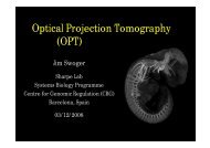
<strong>Optical</strong> <strong>Projection</strong> <strong>Tomography</strong><br />
(<strong>OPT</strong>)<br />
Jim Swoger<br />
Sharpe Lab<br />
Systems Biology Programme<br />
Centre for Genomic Regulation (CRG)<br />
Barcelona, Spain<br />
03/12/2008
Outline<br />
� Motivation<br />
� <strong>OPT</strong>: How It Works<br />
� Depth of Focus Issues<br />
� Image Processing<br />
� Resolution<br />
� Applications, Fixed: - transmission / fluorescence<br />
- disease studies<br />
- mouse limb development<br />
� Applications, Live: - plant<br />
- mouse eye<br />
- mouse limb development<br />
� Conclusions
Motivation
10 �m<br />
100 �m 1mm 1cm 10 cm<br />
CONFOCAL MRI<br />
CELLS TISSUES<br />
Motivation<br />
?<br />
<strong>OPT</strong><br />
ORGANS,<br />
EMBRYOS<br />
ORGANISMS<br />
SPIM, ultramicroscopy, serial sectioning …<br />
Multi-photon, OCT, SHG, structured illum… X-ray CT, ultrasound, …
- E.g. DIC does not relate directly<br />
to physical properties of sample<br />
- “depth info” isn’t real<br />
Motivation<br />
QUALITATIVE vs. QUANTITATIVE imaging<br />
- E.g. fluorescence <strong>OPT</strong>: brightness corresponds<br />
to dye concentration<br />
- Distances/positions can be measured in 3D<br />
projections<br />
slices
SIMPLE<br />
Motivation<br />
Modeling vertebrate limb development<br />
36 hours<br />
PATTERNING<br />
MORPHOGENESIS<br />
DIFFERENTIATION<br />
MECHANICS<br />
COMPLEX
<strong>OPT</strong>: How It Works
<strong>OPT</strong>: How it Works<br />
<strong>Projection</strong> tomography - an X-ray CT scanner<br />
source<br />
detector<br />
Scan Reconstruction<br />
(back-projection)
<strong>OPT</strong>: How it Works<br />
Transmission: Fluorescence: wide-field illum.<br />
“back-projection”<br />
3D RECONSTRUCTION
<strong>OPT</strong>: How it Works<br />
“back-projection”<br />
3D RECONSTRUCTION
<strong>OPT</strong>: How it Works<br />
Same done for<br />
every section<br />
“back-projection”<br />
3D RECONSTRUCTION
<strong>OPT</strong>: How it Works<br />
“back-projection”<br />
3D RECONSTRUCTION
Depth of Focus Issues
Depth of Focus Issues<br />
numerical aperture: NA = n sin�<br />
depth of focus: �z ~ NA -2<br />
lateral resolution: �r ~ NA -1<br />
high low NA<br />
�r<br />
�r<br />
�z �z<br />
Decrease NA:<br />
� �r Depth of Focus (good)<br />
� �z Lateral Resolution<br />
(bad)<br />
�<br />
�
Depth of Focus Issues<br />
numerical aperture: NA = n sin�<br />
depth of focus: �z ~ NA -2<br />
lateral resolution: �r ~ NA -1<br />
Reconstruction:<br />
Decrease NA:<br />
� �r Depth of Focus (good)<br />
� �z Lateral Resolution<br />
(bad)<br />
3D resolution limited by �r<br />
sample size limited by �z
Depth of Focus Issues<br />
High NA Low NA<br />
projections of reconstructions
Image Processing
Pre-Reconstruction Processing<br />
Image Processing for 3D Reconstructions - Details<br />
1) Correction for photo-bleaching during scanning<br />
2) Determination of rotation axis position & orientation<br />
3) Combination of anti-parallel projections<br />
4) Filtered back-projection<br />
?<br />
0°<br />
180°<br />
+ � �
Reconstruction Algorithms<br />
“Simple” Back-<strong>Projection</strong><br />
1. Distribute each projection back<br />
thru sample space,<br />
with the appropriate orientation<br />
2. Sum these back-projections
Reconstruction Algorithms<br />
z<br />
“Simple” Back-<strong>Projection</strong> – Real Data<br />
r<br />
P(r,z,�)
Reconstruction Algorithms<br />
z = z o<br />
z<br />
“Simple” Back-<strong>Projection</strong> – Real Data<br />
r<br />
�<br />
P(r,z,�) r P(r,�,z=zo ) x I(x,y,z=zo )<br />
y
Reconstruction Algorithms<br />
The Fourier Transform:<br />
The Fourier <strong>Projection</strong>/Slice Relationship:<br />
A projection in physical space transforms to a slice in Fourier space.
Reconstruction Algorithms<br />
Physical Space: <strong>Projection</strong>s Fourier Space: Slices<br />
y<br />
Low-density sampling of high frequencies<br />
x<br />
v<br />
High-density sampling of low frequencies<br />
Reconstruction emphasizes low frequencies � low resolution!<br />
u
Reconstruction Algorithms<br />
Filtered Back-projection<br />
z = z o<br />
z<br />
r<br />
�<br />
P(r,z,�) r P(r,�,z=zo ) x I(x,y,z=zo )<br />
Back-projection<br />
y
Resolution & Sample Characteristics
Resolution: <strong>Optical</strong> Clearing of Samples<br />
uncleared transmission cleared, enhanced contrast<br />
- optically, clearing is good.
Resolution Example: Mouse Embryo<br />
3.7 mm<br />
reconstructed <strong>OPT</strong><br />
Mouse embryo<br />
Dehydrated, cleared in BABB<br />
Neurofilament: Alexa 488
Resolution Example: Mouse Embryo<br />
3.7 mm<br />
reconstructed <strong>OPT</strong> reconstructed <strong>OPT</strong>, cropped & zoomed<br />
~ 12 µm isotropic resolution<br />
1.0 mm
Resolution Example: Single-Cell <strong>Imaging</strong><br />
Fauver et al, Opt. Express 13, pp. 4210-4223 (2005)<br />
sub-micron resolution<br />
- Isolated lung fibroblast nucleus<br />
- hematoxylin staining,<br />
(transmission)<br />
- thick section of 3D<br />
reconstruction<br />
- pseudo-colour visualization
Resolution Example: Live Mouse Tissue<br />
400 µm<br />
Reconstructions of fluorescence (implanted beads)<br />
& transmission of an embryonic mouse limb<br />
2<br />
fluorescence transmission overlay<br />
1<br />
3 4<br />
6<br />
5<br />
max-projections<br />
slices
Resolution Example: Live Mouse Tissue<br />
bead 1<br />
bead 3<br />
Bead # Volume [µm^3] bead Mean 2Radius<br />
[µm] Mean Intensity [a.u.] Max Intensity [a.u.]<br />
1 3957 9.81 0.684 34.89<br />
2 44579 22.00 0.643 8.3<br />
3<br />
4<br />
1469<br />
2246<br />
7.05<br />
8.12<br />
normalized 1.532<br />
1.614<br />
225.89<br />
153.02<br />
5 2279 8.16 1.921 275.26<br />
6 1862 7.63 2.529 304.73<br />
anisotropic, context-dependent resolution
Applications: Fixed Sample <strong>Imaging</strong>
Transmission: Whole-mount In Situ<br />
raw <strong>OPT</strong> projection reconstructed slices<br />
<strong>OPT</strong> scan of Sox9 expression (RNA in-situ hybridisation)<br />
E11.5, WT mouse
Transmission: Whole-mount In Situ<br />
<strong>OPT</strong> vs. serial sectioning<br />
raw <strong>OPT</strong><br />
projection<br />
Science 296 pp. 541-545 (2002)<br />
serial section reconstructed<br />
<strong>OPT</strong> section<br />
reconstructed <strong>OPT</strong> section<br />
serial section
Fluorescence: Mouse Embryo<br />
E10.5 mouse embryo<br />
Multi-Channel Fluorescence <strong>OPT</strong><br />
Raw <strong>Projection</strong>s Reconstruction<br />
Red: autofluorescence<br />
Blue: HNF3�, Alexa 488<br />
Green: neurofilament, Cy3<br />
antibody labelling
Fluorescence: Mouse Embryo<br />
E10.5 mouse embryo<br />
Multi-Channel Fluorescence <strong>OPT</strong><br />
Raw <strong>Projection</strong>s Reconstruction<br />
3D Rendering
Arabidopsis Silque, heart-stage embryos<br />
520 µm<br />
Reconstructions from autofluorescence (TXR channel) <strong>OPT</strong> scans<br />
Lee et al, The Plant Cell, 18, pp. 2145-2156 (2006)
Mouse Models of Diabetes<br />
Adult mouse pancreas<br />
White – autofluor.<br />
(GFP filter set)<br />
Red – Islets of Langerhans<br />
(TxR filter set)<br />
Nature Methods 4 pp. 31-33 (2007)
Mouse Models of Diabetes<br />
Normal<br />
Diabetic<br />
Nature Methods 4 pp. 31-33 (2007)
Mouse Models of Immune Response<br />
Lymph nodes: important part of the immune system<br />
lymphocytes introduced to antigens<br />
can become inflamed during infection<br />
mouse peripheral lymph node,<br />
whole-mount staining<br />
White – autofluor.<br />
Green – B-cell follicles, Alexa 488<br />
conjugated anti-B220<br />
www.tki.unibe.ch/stein.htm
Gene Expression Patterning in Mouse<br />
Limb Development<br />
Newman & Frisch (1979)<br />
mid E12<br />
late E12<br />
early E13<br />
Digit patterning during mammalian limb development<br />
Cleared in BABB<br />
Whole-mount in situ for<br />
Sox9 expression
Resolution: <strong>Optical</strong> Clearing of Samples<br />
uncleared transmission cleared, enhanced contrast
Applications: Live Sample <strong>Imaging</strong>
Live <strong>OPT</strong>: Arabidopsis Development<br />
4 hours<br />
100 µm<br />
9<br />
24<br />
49<br />
Reconstructions from transmission <strong>OPT</strong> scans<br />
Lee et al, The Plant Cell, 18, pp. 2145-2156 (2006)<br />
72<br />
High magnification slices, @ 30 hours
The Bioptonics <strong>OPT</strong> System<br />
More <strong>OPT</strong> info: U.K. Medical Research Council:<br />
www.bioptonics.com
Live Mammalian <strong>OPT</strong>: Hardware<br />
Live <strong>OPT</strong> machine:<br />
- Built inside a climate-controlled chamber<br />
- All alignment & sample manipulation (x, y, z, roll, pitch, yaw) controls<br />
are external
Live Mammalian <strong>OPT</strong>: Hardware<br />
XY translation stage<br />
magnet<br />
concave surface<br />
oil
Live <strong>OPT</strong>: Mouse Lens Induction<br />
Mouse embryo, E9.5<br />
Pax6-GFP in ectoderm, prospective retina, forebrain<br />
Raw <strong>OPT</strong> projections<br />
Prospective retina bulges inward due to growth of lens<br />
Reconstructed slice, t = 0<br />
t = +6 hours
Applications: Mouse Limb Development
Goals<br />
Quantitative modeling of mammalian organ development<br />
Specifically, can we understand the processes that turn Ainto<br />
B<br />
i.e. Mouse limb development (E10.75 � E12.25)<br />
A B<br />
36 hours<br />
To construct a 4D finite-element model<br />
we require quantitative data on:<br />
1) gene expression patterning 2) morphology 3) local tissue motion
Quantifying Gene Expression &<br />
Morphology<br />
Dynamic gene expression patterns in 4D?...<br />
Boot et al, Nat. Methods, 5, pp. 609-612 (2008)
Quantifying Gene Expression &<br />
Morphology<br />
t 0 (E11.5)<br />
Scleraxis-GFP transgenic mouse line<br />
Ronen Schweitzer<br />
Oregon, USA<br />
Dynamic gene expression patterns in 4D?...<br />
Boot et al, Nat. Methods, 5, pp. 609-612 (2008)
Quantifying Gene Expression &<br />
Morphology<br />
t 0 (E11.5)<br />
Scleraxis-GFP transgenic mouse line<br />
Ronen Schweitzer<br />
Oregon, USA<br />
t 0 + 19 hours<br />
Dynamic gene expression patterns in 4D?... .<br />
Boot et al, Nat. Methods, 5, pp. 609-612 (2008)
Quantifying Gene Expression &<br />
Morphology<br />
E16.5 mouse embryo: scans through <strong>OPT</strong> reconstructions<br />
transmission fluorescence overlay
Tracking Ectodermal Motion<br />
Can only track shape changes<br />
Cannot track tissue movements<br />
Require Landmarks<br />
the model we want to make<br />
the data we have (morphology)
Tracking Ectodermal Motion<br />
Fluorescent beads attached to limb surface<br />
Boot et al, Nat. Methods, 5, pp. 609-612 (2008)<br />
raw <strong>OPT</strong> projections<br />
1 time-point; multiple views
Tracking Ectodermal Motion<br />
Fluorescent beads attached to limb surface<br />
Boot et al, Nat. Methods, 5, pp. 609-612 (2008)<br />
raw <strong>OPT</strong> projections<br />
time-series; single view
Tracking Ectodermal Motion<br />
<strong>OPT</strong> reconstructions<br />
vectors connecting time-points<br />
Boot et al, Nat. Methods, 5, pp. 609-612 (2008)<br />
raw <strong>OPT</strong> projections<br />
time-series; single view
Tracking Ectodermal Motion<br />
<strong>OPT</strong> reconstructions<br />
vectors connecting time-points<br />
Boot et al, Nat. Methods, 5, pp. 609-612 (2008)<br />
Overlay multiple experiments
Tracking Ectodermal Motion<br />
Analyze: “vortices” are apparent<br />
Interpolate for uniform coverage:<br />
Green: “original” bead vectors<br />
Red: Interpolated<br />
Boot et al, Nat. Methods, 5, pp. 609-612 (2008)<br />
Overlay multiple experiments
Tracking Volumetric Growth<br />
Tamoxifen-inducible Cre-Lox EYFP stochastic clonal labelling<br />
Arques et al, Development, 134, pp. 3713-3722 (2007)
Tracking Volumetric Growth<br />
reconstuction, 1st clone tracking<br />
time-point reconstuction, time-series
Quantitative Modeling<br />
Mesh for a Finite Element model<br />
of a limb bud<br />
Color encodes proliferation rate<br />
(blue high; red low)<br />
For the model we need:<br />
Gene Expression: what genes are<br />
expressed in what regions<br />
Morphology: the limb shape<br />
Tissue Motion: node movements<br />
between iterations<br />
Q: Given morphologies at t 1 & t 2 , what tissue motions are consistent with this?<br />
Q: Can proliferation rates alone account for measured morphology?
Conclusions
Acknowledgements<br />
Sharpe Lab<br />
Jean-François Colas – limb bud culturing<br />
Laura Quintana – fixed <strong>OPT</strong><br />
Sahdia Raja – Sox9 imaging, proliferation data<br />
Henrik Westerberg – visualization, post-processing<br />
Bernd Böhm – finite element modelling<br />
Centre for Genomic Regulation, Barcelona, Spain<br />
Marit Boot – limb development<br />
Human Genetics <strong>Unit</strong>, Medical Research Council<br />
Edinburgh, U.K.<br />
Miguel Torres & Juan José Sanz – live <strong>OPT</strong> development<br />
CNB, CSIC, Madrid, Spain – Cre-Lox EYFP mouse<br />
Ronen Schweitzer – Scx-GFP mice<br />
Shriners Hospital for Children, Portland, U.S.A.<br />
Ulf Ahlgren – pancreatic collaborations<br />
Umeå U., Sweden<br />
Jens Stein – lymphatic collaborations<br />
U. Bern, Switzerland