Appendix A Abbreviations used
Appendix A Abbreviations used
Appendix A Abbreviations used

Create successful ePaper yourself
Turn your PDF publications into a flip-book with our unique Google optimized e-Paper software.
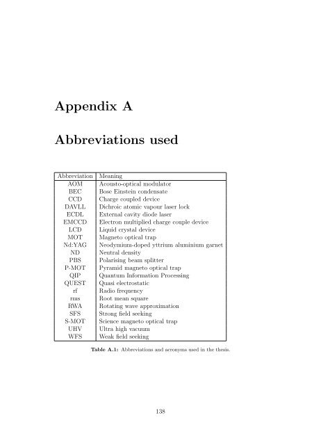
<strong>Appendix</strong> A<br />
<strong>Abbreviations</strong> <strong>used</strong><br />
Abbreviation Meaning<br />
AOM Acousto-optical modulator<br />
BEC Bose Einstein condensate<br />
CCD Charge coupled device<br />
DAVLL Dichroic atomic vapour laser lock<br />
ECDL External cavity diode laser<br />
EMCCD Electron multiplied charge couple device<br />
LCD Liquid crystal device<br />
MOT Magneto optical trap<br />
Nd:YAG Neodymium-doped yttrium aluminium garnet<br />
ND Neutral density<br />
PBS Polarising beam splitter<br />
P-MOT Pyramid magneto optical trap<br />
QIP Quantum Information Processing<br />
QUEST Quasi electrostatic<br />
rf Radio frequency<br />
rms Root mean square<br />
RWA Rotating wave approximation<br />
SFS Strong field seeking<br />
S-MOT Science magneto optical trap<br />
UHV Ultra high vacuum<br />
WFS Weak field seeking<br />
Table A.1: <strong>Abbreviations</strong> and acronyms <strong>used</strong> in the thesis.<br />
138
<strong>Appendix</strong> B<br />
Symbol definitions<br />
In Table B.1 the majority of the symbols <strong>used</strong> in the thesis are tabulated in<br />
alphabetical order with their definition. Some symbols have dual definitions<br />
but the context is sufficient to work out which one is relevant. The rules for<br />
subscripts are: i denotes an initial value; x, y, z are the Cartesian components;<br />
r is the radial component. Vectors have a bold font. Primes are <strong>used</strong> in four<br />
contexts: to distinguish ‘thin lens’ times from their ‘thick lens’ counterparts; to<br />
indicate excited states; to distinguish currents in coils and bars; to distinguish<br />
harmonic trap and laser guide angular frequencies.<br />
Symbol Physical meaning<br />
α Polarisability<br />
α0 Scalar polarisability<br />
α2 Tensor polarisability<br />
a Coil radius<br />
a0 Bohr radius<br />
a0 Acceleration due to B-field gradient<br />
aF Full Biot-Savart lens acceleration<br />
aH Acceleration from harmonic fit to B-field<br />
aS Scattering length<br />
A, B, C, D ABCD-matrix elements<br />
Ahfs Hyperfine structure constant<br />
β Viscosity constant<br />
B(x, y, z) Magnetic field magnitude<br />
B(x, y, z) Magnetic field<br />
B0 Bias field of magnetic field<br />
B1 Gradient of magnetic field<br />
B2 Curvature of magnetic field<br />
Bhfs Hyperfine structure constant<br />
BZ(x, y, z) Magnetic field of current bar along z-axis<br />
Table B.1: Symbols <strong>used</strong> and their meanings.<br />
139
<strong>Appendix</strong> B. Symbol definitions 140<br />
Symbol Physical meaning<br />
χ Loading efficiency<br />
c Speed of light<br />
∆ Angular detuning (∆ = 2πδ)<br />
d Grating line spacing<br />
ɛ(R, Z) Harmonicity<br />
ɛ0<br />
Permittivity of free space<br />
η η = µ0NI/2<br />
E Energy<br />
E(k) Complete elliptic integral (1st kind)<br />
E Electric field<br />
Ehfs<br />
Hyperfine interaction matrix<br />
f Focal length of lens<br />
F Fraction of atoms in the Gaussian focus<br />
F Total atomic angular momentum<br />
Scattering forces in a MOT<br />
F±,tot<br />
FDip<br />
Dipole force<br />
Γ Natural line width. Excited state decay rate.<br />
Γ(a, b, c) Generalised incomplete gamma function<br />
Γsc(r) Scattering rate<br />
g Acceleration due to gravity<br />
gn<br />
Gain of photodiode circuit<br />
G Total transimpedance<br />
h Height<br />
� Plank’s constant/2π<br />
I Identity matrix<br />
I Current in coil<br />
I ′ Current in bar<br />
I(r) Intensity<br />
IAH Current in the opposite sense (2IAH = I1 − I2)<br />
IH Current in the same sense (2IAH = I1 + I2)<br />
Nuclear quantum number<br />
In<br />
Isat<br />
Saturation intensity<br />
J Total electronic angular momentum<br />
κ fractional solid angle<br />
k Substitution <strong>used</strong> in circular coil expression (eqn. (4.10))<br />
k Wavevector<br />
kB<br />
Boltzmann’s constant<br />
K Sum of quantum numbers (eqn. (2.17))<br />
K(k) Complete elliptic integral (2nd kind)<br />
λ Focusing parameter (single-impulse)<br />
λ1,2 Focusing parameter (double-impulse)<br />
λC Wavelength of cooling laser<br />
λT Wavelength of trapping laser<br />
L = l/a Scaled length of current bar in baseball lens<br />
µ0 Permeability of free space<br />
µB Bohr magneton<br />
m Mass<br />
Magnetic quantum number<br />
mF
<strong>Appendix</strong> B. Symbol definitions 141<br />
Symbol Physical meaning<br />
M System matrix<br />
Mag Magnification<br />
n Density OR Diffraction order<br />
N Number of atoms OR coil turns<br />
Φ(r, p) Phase space distribution<br />
p Radial momentum<br />
p Dipole moment<br />
P Laser power<br />
PMOT Power emitted by MOT<br />
PPD Power measured by photodiode<br />
q Integral substitution (Section 3.3)<br />
Q Q-matrix<br />
r Polar coordinate<br />
σ Spatial standard deviation<br />
σel Collision cross section<br />
σv Velocity standard deviation<br />
σR Initial isotropic spatial standard deviation<br />
σV Initial isotropic velocity standard deviation<br />
S = s/a Scaled coil separation<br />
S Photodiode sensitivity<br />
τ Pulse duration (single-impulse)<br />
τ1,2 Pulse duration (double-impulse)<br />
θ Angle of diffraction<br />
t Time<br />
t1,2 Time of lens pulse<br />
T Temperature<br />
TD Doppler limit<br />
T Total focusing time<br />
Tosc Laser guide oscillation period<br />
Tr Transmission<br />
UDip Dipole potential<br />
vzi Vertical launch velocity<br />
v Velocity<br />
V Photodiode voltage<br />
ω Lens angular frequency (single-impulse)<br />
ω ′ Harmonic trap angular frequency<br />
ω0 Atomic transition angular frequency<br />
ω1,2 Lens angular frequency (double-impulse)<br />
ωrL Laser light’s angular frequency<br />
w(z) 1/e2 intensity radius<br />
w0 Beam waist<br />
W = w/a Scaled length of current bar in baseball lens<br />
ξ = σz/σr Cloud aspect ratio<br />
x, y, z Cartesian coordinate<br />
X, Y, Z, R Scaled position coordinate (eg. X = x/a)<br />
z0 Focal point<br />
zc Vertical position of the lens centre<br />
Rayleigh length<br />
zR
<strong>Appendix</strong> C<br />
Values and constants<br />
Quantity Symbol Value Unit<br />
Acceleration due to gravity g 9.807 m s −2<br />
Atomic mass unit u 1.661 × 10 −27 kg<br />
Boltzmann’s constant kB 1.381 × 10 −23 J K −1<br />
Bohr magneton µB 9.274 × 10 −24 J T −1<br />
Bohr radius a0 5.292 × 10 −11 m<br />
Electron charge e 1.602 × 10 −19 C<br />
Electron mass me 9.109 × 10 −31 kg<br />
Permeability of free space µ0 4π × 10 −7 N A −2<br />
Permittivity of free space ɛ0 8.854 × 10 −12 F m −1<br />
Planks constant/2π � 1.055 × 10 −34 J s<br />
Speed of light in a vacuum c 2.999 × 10 8 m s −1<br />
Rubidium natural linewidth [126] Γ 2π × 5.9 MHz<br />
Hyperfine structure constants [132] Ahfs 2π × 25.009 MHz<br />
Bhfs 2π × 25.88 MHz<br />
D2 line wavelength [123] λC 780.24 nm<br />
Table C.1: Values and constants <strong>used</strong>. Values for the fundamental constants<br />
are the CODATA recommended values [190].<br />
142
<strong>Appendix</strong> D<br />
Atomic structure of Rb<br />
F’=4<br />
F’=3<br />
F’=2<br />
F’=1<br />
F=3<br />
F=2<br />
85 Rb<br />
120.96 MHz<br />
63.42 MHz<br />
29.26 MHz<br />
3,036 MHz<br />
5p P<br />
2<br />
3/2<br />
780.24 nm<br />
5s S<br />
2<br />
½<br />
87 Rb<br />
266.65 MHz<br />
156.88 MHz<br />
72.19 MHz<br />
6,835 MHz<br />
F’=3<br />
F’=2<br />
F’=1<br />
F’=0<br />
F=2<br />
F=1<br />
Figure D.1: The hyperfine energy level diagram on the D2 line for the 85 Rb<br />
and 87 Rb isotopes [191, 192].<br />
143
<strong>Appendix</strong> E<br />
Collision rate<br />
Following the approach taken in ref. [154] to calculate the collision rate within<br />
a MOT. The density of a spherically symmetric Gaussian spatial distribution<br />
with N atoms and a spatial standard deviation of σR is:<br />
where the peak density is:<br />
�<br />
n(r) = n0 exp − x2 + y2 + z2 2σR 2<br />
�<br />
, (E.1)<br />
n0 =<br />
The spatially averaged elastic collision rate is:<br />
Γel = σel<br />
= σel n0<br />
N<br />
(2π) 3/2 . (E.2)<br />
σR<br />
3<br />
� n 2 (r)vrel d 3 r<br />
� n(r) d 3 r = σel〈n〉〈vrel〉,<br />
�<br />
3kBT<br />
, (E.3)<br />
4m<br />
where the density-weighted density for a Gaussian distribution is 〈n〉 = n0/ √ 8<br />
and the rms average velocity between atoms of mass m is 〈vrel〉 = � 6kBT /m.<br />
The dominant collision at ultracold temperatures is s-wave elastic collisions:<br />
σel =<br />
8πaS 2<br />
1 + k2 , (E.4)<br />
aS<br />
2<br />
where k = √ 2πmkBT /� and aS is the scattering length. Combining eqns. (E.2),<br />
(E.3) and (E.4), and using the experimentally measured 85 Rb background scat-<br />
tering length aS = −433 a0 from ref. [193], the MOT average collision rate is:<br />
Γel = 3 s −1 .<br />
144
<strong>Appendix</strong> F<br />
Mathematica computer code<br />
Below is an example Mathematica computer code that calculates the trajectories<br />
of atoms passing along a laser guide.<br />
Define fundamental constants.<br />
Bohr �0.5292 �10 �10 ;<br />
c �2.999 �10 8 ;g�9.807;<br />
kb �1.381 �10 �23 ; m �85 �1.661 �10 �27 ;<br />
Calculate the laser beam potential using the ground state polarisability of Rb.<br />
waist �250 �10 �6 ;z0 �0.0;<br />
� �1064 �10 �9 ;ray � �waist 2 � �;<br />
power �19;<br />
�z �z0�2<br />
w1�z_�:�waistSqrt�1 � ���������������� ������� �;<br />
ray 2<br />
2 �power<br />
int�r_, z_� � ���������������� ������� Exp��2<br />
� r 2<br />
�� ����������������<br />
���<br />
�;<br />
2 �w1�z� �w1�z�<br />
�<br />
�0 �693.5;<br />
�0 �4�Pi<br />
U0 � ���������������� ��������� �Bohr<br />
2c<br />
3 ;<br />
U�x_, y_, z_�:� �U0int� ����������������<br />
x2 �y2, z�;<br />
Calculate the acceleration due to the dipole potential. The dummy variables <strong>used</strong> in the differentiation<br />
are replaced with the correct coordinate at the end.<br />
��Calculates acceleration on atoms��<br />
accx�x_, y_, z_� � �D�U��, y, z�, �� �m �. �� �x� ��Evaluate ��Simplify;<br />
accy�x_, y_, z_� � �D�U�x, �, z�, �� �m �. �� �y� ��Evaluate ��Simplify;<br />
accz�x_, y_, z_� � �D�U�x, y, ��, �� �m �. �� �z� ��Evaluate ��Simplify;<br />
145
<strong>Appendix</strong> F. Mathematica computer code 146<br />
Setup the Gaussian spatial and velocity distributions for the atomic sample. Table "mix1" contains<br />
the x-direction data, "mix2" y-direction and "mix3" z-direction.<br />
atoms �25;<br />
cloudradius �0.0002;<br />
temp �20 �10 �6 ;thermalvel �Sqrt�kb � �temp �m��;<br />
��"Statistics`NormalDistribution`"<br />
ndistpos:�Random�NormalDistribution�0, cloudradius��;<br />
ndistvel:�Random�NormalDistribution�0, thermalvel��;<br />
xcom �10 �8 ;xvcom �0;ycom �10 �8 ;yvcom �0;zcom �0;<br />
mix1 �Table��xcom �ndistpos, xvcom �ndistvel�, �atoms��;<br />
mix2 �Table��ycom �ndistpos, yvcom �ndistvel�, �atoms��;<br />
mix3 �Table��zcom �ndistpos, ndistvel�, �atoms��;<br />
Calculate the launch velocity and flight duration based on a given height.<br />
height �0.22;<br />
zvcom �Sqrt�2 �g�height�;<br />
tfocus �Sqrt��2 �height� �g�;<br />
tmx �0.02 �tfocus;<br />
The equations of motion for the system. Mathematica produces interpolating functions for each<br />
atom. Only the x-direction table is generated in this example.<br />
Clear�Coord�;<br />
Coord�xpos_, xvel_, ypos_, yvel_, zpos_, zvel_�:�<br />
Coord�xpos, xvel, ypos, yvel, zpos, zvel� �<br />
NDSolve��vx'�t� �accx�x�t�, y�t�, z�t��, x'�t� �vx�t�, vx�0� �xvel, x�0� � xpos,<br />
vy'�t� �accy�x�t�, y�t�, z�t��, y'�t� �vy�t�, vy�0� �yvel, y�0� �ypos,<br />
vz'�t� �accz�x�t�, y�t�, z�t�� �g, z'�t� � vz�t�, vz�0� �zvel, z�0� �zpos�,<br />
�x�t�, vx�t�, y�t�, vy�t�, z�t�, vz�t��, �t, 0, tmx�, MaxSteps �10000�;<br />
xtraj �Table��x�t� � �xvcom �t �xcom� �.<br />
Coord�mix1��shelf, 1��, mix1��shelf, 2��, mix2��shelf, 1��, mix2��shelf, 2��,<br />
mix3��shelf, 1��, mix3��shelf, 2�� �zvcom����1��, �shelf, 1, atoms��;<br />
Plots the x position against time and generates a data table that can be further analysed or exported.<br />
Plot�Evaluate�xtraj�, �t, 0, tmx��;dt �2000;<br />
xstatdata �Table�Evaluate�Flatten�xtraj��, �t, 0, tmx, 1 �dt��;
<strong>Appendix</strong> G<br />
Fibre optic alignment<br />
Due to the elliptical cross-section, polarisation preserving fibre optics will only<br />
function properly if the incoming linearly polarised light is aligned to one of the<br />
two orthogonal axes running along the fibre (semi-major or semi-minor axis).<br />
If the axes are not marked, a simple way to determine the correct polarisation<br />
is outlined in this <strong>Appendix</strong>. The experimental setup is shown in Figure G.1.<br />
�/2 Fibre optic �/4<br />
PBS<br />
Photo<br />
diode<br />
Figure G.1: Experimental setup <strong>used</strong> to align the polarisation of light going<br />
into the fibre optics. The λ/4 waveplate is only <strong>used</strong> when converting the light<br />
into circular polarisation.<br />
The initial alignment does not make use of the λ/4 waveplate. A rotatable<br />
polarising beam splitting (PBS) cube is <strong>used</strong> with a either a photodiode or<br />
power meter (Coherent Field Master) to analyse the polarisation of the light<br />
exiting the fibre. The PBS cube is rotated to obtain values for the maximum<br />
and minimum powers measured by the photodiode. The signature of linear light<br />
exiting from the fibre optic is that the ratio of maximum power to minimum<br />
power is maximised. The initial λ/2 waveplate is <strong>used</strong> to rotate the polarisation<br />
of the light entering the fibre. A plot of the max/min power ratio against<br />
λ/2 waveplate rotation angle is given in Figure G.2 (a). As expected from<br />
the 2θ rotation property of the waveplate, one finds a maximum every 45 ◦ . A<br />
close-up of the first maximum is shown in Figure G.2 (b).<br />
147
<strong>Appendix</strong> G. Fibre optic alignment 148<br />
���<br />
�������������<br />
���<br />
���<br />
���<br />
���<br />
���<br />
���<br />
�<br />
� �� �� �� �� ��� ��� ��� ��� ���<br />
���������������<br />
���<br />
�������������<br />
���<br />
���<br />
���<br />
���<br />
���<br />
���<br />
�<br />
� � �� �� ��<br />
���������������<br />
Figure G.2: The maximum to minimum power ratio is plotted against<br />
λ/2 waveplate angle. Plot (b) examines the first maximum in (a).<br />
The correct angle of a λ/4 waveplate to convert linear light into circular polar-<br />
isation can be similarly determined. In this case the λ/4 waveplate is rotated<br />
and the ratio of minimum to maximum power is plotted, see Figure G.3. In<br />
this case the waveplate is set to one of the maximum angles.<br />
�������������<br />
���<br />
���<br />
���<br />
���<br />
���<br />
���<br />
� �� �� �� �� ��� ��� ��� ��� ���<br />
���������������<br />
Figure G.3: The minimum to maximum power ratio is plotted against<br />
λ/4 waveplate angle.<br />
Another method to align the linear polarisation into the fibre that does not<br />
involve rotating the PBS cube is to plot the peak-to-peak noise on the pho-<br />
todiode voltage against the rotation angle of the λ/2 waveplate. During the<br />
measurement, the fibre is deliberately stressed and heated by gently massaging<br />
the fibre. When the light is propagating down one of the orthogonal axes the<br />
effect of the perturbation is minimised and is seen by a dramatic reduction in<br />
the photodiode noise.
<strong>Appendix</strong> H<br />
Knife edge measurements<br />
A crude, but nonetheless effective, method of measuring a laser beam’s profile<br />
is now described. A knife edge is translated through the beam’s cross-section.<br />
The resulting change in power as a function of knife edge position allows the<br />
1/e 2 beam radius w(z) to be calculated (see Section 3.1). Multiple readings at<br />
different z positions allow a full description of the laser beam’s spatial profile.<br />
Treating the x- and y-direction beam waists as being independent i.e. an ellip-<br />
tical beam profile, the total power in the beam is given by integrating eqn. (3.1)<br />
on page 26:<br />
Ptotal =<br />
� ∞ � ∞<br />
−∞<br />
−∞<br />
I(x, y)dydx = π<br />
2 I0wxwy. (H.1)<br />
As the knife edge moves across the beam in the x-direction the power measured<br />
at the photodiode varies as:<br />
P (X) = Ptotal −<br />
� X<br />
−∞<br />
� ∞<br />
−∞<br />
After integration and substituting in the error function:<br />
I(x, y)dydx. (H.2)<br />
erf(u) = 2<br />
� u<br />
√ e<br />
π 0<br />
−u2<br />
du , (H.3)<br />
the power measured by the photodiode vs. knife edge position, X, will have the<br />
following form:<br />
P (X) = Ptotal<br />
2<br />
� �√ ��<br />
2 X<br />
1 − erf<br />
. (H.4)<br />
An example of this measurement can be found in Figure H.1. The data were<br />
recorded by translating the knife edge through one of the three arms of the<br />
149<br />
wx
<strong>Appendix</strong> H. Knife edge measurements 150<br />
S-MOT cooling beams; see Figure 8.22. A fit to the data gives the 1/e 2 beam<br />
radius as 7.5 mm and the peak intensity as 7.1 mW/cm 2 .<br />
����������<br />
�<br />
�<br />
�<br />
�<br />
�<br />
�<br />
�<br />
� �� �� �� �� �� �� �� �� ��<br />
�����������<br />
Figure H.1: Knife edge measurement of the S-MOT laser beam.
Bibliography<br />
[1] S. Chu, C. N. Cohen-Tannoudji, and W. D. Phillips, Rev. Mod. Phys. 70, 707<br />
(1998).<br />
[2] C. S. Adams and E. Riis, Prog. Quant. Electr. 21, 1 (1997).<br />
[3] http://www.uibk.ac.at/exphys/ultracold/atomtraps.html.<br />
[4] E. A. Cornell and C. E. Wieman, Rev. Mod. Phys. 74, 875 (2002).<br />
[5] W. Ketterle, Rev. Mod. Phys. 74, 1131 (2002).<br />
[6] B. DeMarco and D. S. Jin, Science 285, 1703 (1999).<br />
[7] D. Budker et al., Rev. Mod. Phys. 74, 1153 (2002).<br />
[8] B. Levy, Phys. Today 44, 17 (1991).<br />
[9] J. Helmcke, F. Riehle, A. Witte, and T. Kisters, Phys. Scripta T40, 32 (1992).<br />
[10] F. G. Major, The Quantum Beat: The Physical Principles of Atomic Clocks<br />
(Springer-Verlag, New York, 1998).<br />
[11] C. Salomon et al., C. R. Acad. Sci. Paris. Serie IV, 1313 (2001).<br />
[12] H. J. Briegel, T. Calarco, D. Jaksch, J. Cirac, and P. Zoller, J. Mod. Opt. 47,<br />
415 (2000).<br />
[13] M. A. Nielson and I. L. Chuang, Quantum Computation and Quantum Information<br />
(CUP, Cambridge, 2000).<br />
[14] A. M. Steane, Appl. Phys. B. 64 (1997).<br />
[15] C. S. Adams, M. Sigel, and J. Mlynek, Phys. Rep. 240, 143 (1994).<br />
[16] V. I. Balykin and W. Jhe, J. Korean Phys. Soc. 37, 654 (2000).<br />
[17] N. F. Ramsey, Molecular beams (Oxford, OUP, 1985).<br />
[18] L. Estermann and O. Stern, Z. Phys. 61, 95 (1930).<br />
[19] O. R. Frish and O. Stern, Z. Phys 84, 430 (1933).<br />
[20] D. W. Keith, M. L. Schattenburg, H. I. Smith, and D. E. Pritchard, Phys. Rev.<br />
Lett. 61, 1580 (1988).<br />
[21] O. Carnal, M. Sigel, T. Sleator, H. Takuma, and J. Mlynek, Phys. Rev. Lett.<br />
67, 3231 (1991).<br />
151
Bibliography 152<br />
[22] J. J. Berkhout, O. J. Luiten, I. D. Setija, T. Mizusaki, and J. T. M. Walraven,<br />
Phys. Rev. Lett. 63, 1689 (1989).<br />
[23] B. Holst and W. Allison, Nature 390, 244 (1997).<br />
[24] R. J. Wilson, B. Holst, and W. Allison, Rev. Sci. Instrum. 70, 2960 (1999).<br />
[25] J. P. Gordon, H. J. Zeiger, and C. Townes, Phys. Rev. 99, 1264 (1955).<br />
[26] J. A. Maddi, T. P. Dinneen, and H. Gould, Phys. Rev. A 60, 3882 (1999).<br />
[27] H. B. Bethlem and G. Meijer, Int. Rev. Phys. Chem. 22, 73 (2003).<br />
[28] M. R. Tarbutt et al., Phys. Rev. Lett. 92, 173002 (2004).<br />
[29] H. L. Bethlem et al., J. Phys. B 39, R263 (2006).<br />
[30] J. J. Hudson, B. E. Sauer, M. R. Tarbutt, and E. A. Hinds, Phys. Rev. Lett.<br />
89, 023003 (2002).<br />
[31] E. A. Hinds and I. G. Hughes, J. Phys. D 32, R119 (1999).<br />
[32] T. M. Roach et al., Phys. Rev. Lett. 75, 629 (1995).<br />
[33] A. I. Sidorov et al., Quantum Semiclass. Opt. 8, 713 (1996).<br />
[34] D. C. Lau et al., Eur. Phys. J. D 5, 193 (1999).<br />
[35] I. G. Hughes, P. A. Barton, T. M. Roach, M. G. Boshier, and E. A. Hinds, J.<br />
Phys. B 30, 647 (1997).<br />
[36] I. G. Hughes, P. A. Barton, T. M. Roach, and E. A. Hinds, J. Phys. B 30, 2119<br />
(1997).<br />
[37] I. G. Hughes, T. Darlington, and E. A. Hinds, J. Phys. B 34, 2869 (2001).<br />
[38] C. V. Saba et al., Phys. Rev. Lett. 82, 468 (1999).<br />
[39] D. Kadio, O. Houde, and L. Pruvost, Europhys. Lett. 54, 417 (2001).<br />
[40] I. Bloch, M. Köhl, M. Greiner, T. W. Hänsch, and T. Esslinger, Phys. Rev.<br />
Lett. 87, 030401 (2001).<br />
[41] A. S. Arnold, C. MacCormick, and M. G. Boshier, Phys. Rev. A 65, 031601(R)<br />
(2002).<br />
[42] A. S. Arnold, C. MacCormick, and M. G. Boshier, J. Phys. B 37, 485 (2004).<br />
[43] P. Rosenbusch, B. V. Hall, I. G. Hughes, C. V. Saba, and E. A. Hinds, Phys.<br />
Rev. A 61, 031404 (2000).<br />
[44] P. Rosenbusch, B. V. Hall, I. G. Hughes, C. V. Saba, and E. A. Hinds, Appl.<br />
Phys. B 70, 709 (2000).<br />
[45] H. Friedburg and W. Paul, Naturwissenschaft 38, 159 (1951).<br />
[46] H. Friedburg, Z. Phys. 130, 493 (1951).<br />
[47] H. Metcalf, W. Philips, and J. Prodan, Bull. Am. Phys. Soc. 29, 785 (1984).<br />
[48] W. G. Kaenders et al., Phys. Rev. A 54, 5067 (1996).
Bibliography 153<br />
[49] E. A. Cornell, C. Monroe, and C. E. Wieman, Phys. Rev. Lett. 67, 2439 (1991).<br />
[50] E. Maréchal et al., Eur. Phys. J. D 2, 195 (1998).<br />
[51] E. Maréchal et al., Phys. Rev. A 59, 4636 (1999).<br />
[52] T. Miossec, R. Barbé, J. C. Keller, and O. Gorceix, Opt. Commun. 209, 349<br />
(2002).<br />
[53] S. H. Myrskog, J. K. Fox, H. S. Moon, J. B. Kim, and A. M.Steinberg, Phys.<br />
Rev. A 61, 053412 (2000).<br />
[54] T. Aoki, T. Kato, Y. Tanami, and H. Nakamatsu, Phys. Rev. A 73, 063603<br />
(2006).<br />
[55] S. Goldberg et al., Phys. Rev. A 68, 043410 (2003).<br />
[56] M. Greiner, I. Bloch, T. W. Hänsch, and T. Esslinger, Phys. Rev. A 63, 031401<br />
(2001).<br />
[57] H. J. Lewandowski, D. M. Harber, D. L. Whitaker, and E. A. Cornell, J. Low<br />
Temp. Phys. 132, 309 (2003).<br />
[58] J. Goldwin, M. L. Olsen, B. Newman, B. D. DePaola, and D. S. Jin, Phys.<br />
Rev. A 70, 021 601(R) (2004).<br />
[59] K. Nakagawa, Y. Suzuki, M. Horikoshi, and J. Kim, Appl. Phys. B 81, 791<br />
(2005).<br />
[60] T. Lahaye, G. Reinaudi, Z. Wang, A. Couvert, and D. Guéry-Odelin,<br />
arXiv:cond-mat , 0605302 (2006).<br />
[61] T. W. Hansch and A. L. Schawlow, Opt. Comm. 13, 68 (1975).<br />
[62] D. Wineland and H. Dehmelt, Bull. Am. Phys. Soc. 20, 637 (1975).<br />
[63] S. Chu, L. Hollberg, J. E. Bjorkholm, A. Cable, and A. Ashkin, Phys. Rev.<br />
Lett 55, 48 (1985).<br />
[64] E. L. Raab, M. Prentiss, A. Cable, S. Chu, and D. E. Pritchard, Phys. Rev.<br />
Lett. 59, 2631 (1987).<br />
[65] G. A. Askar’yan, Sov. Phys. JETP 15, 1088 (1962).<br />
[66] V. S. Letokhov, JETP Lett. 7, 272 (1968).<br />
[67] A. Ashkin, Phys. Rev. Lett. 24, 156 (1970).<br />
[68] A. Ashkin, Phys. Rev. Lett. 40, 729 (1978).<br />
[69] J. E. Bjorkholm, R. E. Freeman, A. A. Ashkin, and D. B. Pearson, Phys. Rev.<br />
Lett. 41, 1361 (1978).<br />
[70] S. Chu, J. E. Bjorkholm, A. Ashkin, and A. Cable, Phys. Rev. Lett 56, 314<br />
(1986).<br />
[71] T. Sleator, T. Pfau, V. Balykin, O. Carnal, and J. Mlynek, Appl. Phys. B 54,<br />
375 (1992).<br />
[72] M. A. Kasevich, D. S. Weiss, and S. Chu, Opt. Lett. 15, 607 (1990).
Bibliography 154<br />
[73] C. G. Aminoff et al., Phys. Rev. Lett. 71, 3083 (1993).<br />
[74] K. Szymaniec, H. J. Davies, and C. S. Adams, Europhys. Lett. 45, 450 (1999).<br />
[75] H. J. Davies and C. S. Adams, J. Phys. B 33, 4079 (2000).<br />
[76] H. J. Davies, K. Szymaniec, and C. S. Adams, Phys. Rev. A 62, 013412 (2000).<br />
[77] L. Pruvost, D. Marescaux, O. Houde, and H. T. Duong, Opt. Comm. 166, 199<br />
(1999).<br />
[78] H. R. Noh, X. Xu, and W. Jhe, Adv. At. Mol. Opt. Phys. 48, 153 (2002).<br />
[79] D. P. Rhodes et al., J. Mod. Opt. 53, 547 (2006).<br />
[80] M. J. Renn et al., Phys. Rev. Lett. 75, 3253 (1995).<br />
[81] M. J. Renn, E. A. Donley, E. A. Cornell, C. E. Wieman, and D. Z. Anderson,<br />
Phys. Rev. A 53, R648 (1996).<br />
[82] M. J. Renn, A. A. Zozulya, E. A. Donely, E. A. Cornell, and D. Z. Anderson,<br />
Phys. Rev. A 55, 3684 (1997).<br />
[83] H. Ito, K. Sakaki, M. Ohtsu, and W. Jhe, Appl. Phys. Lett. 70, 2496 (1997).<br />
[84] T. L. Gustavson et al., Phys. Rev. Lett. 88, 020401 (2001).<br />
[85] J. P. Dowling and J. Gea-Banacloche, Adv. At. Mol. Opt. Phys. 36, 1 (1996).<br />
[86] V. I. Balykin, Adv. At. Mol. Opt. Phys. 41, 181 (1999).<br />
[87] R. Grimm, M. Weidemuller, and Y. B. Ovchinnikov, Adv. Atom. Mol. Phys.<br />
42, 95 (2000).<br />
[88] J. D. Miller, R. A. Cline, and D. J. Heinzen, Phys. Rev. A 47, R4567 (1993).<br />
[89] T. Takekoshi, J. R. Yeh, and R. J. Knize, Opt. Comm. 114, 421 (1995).<br />
[90] T. Takekoshi and R. J. Knize, Optics Lett. 21, 77 (1996).<br />
[91] A. Mosk, S. Kraft, and M. Mudrich, Appl. Phys. B 73, 791 (2001).<br />
[92] M. Mudrich et al., Phys. Rev. Lett. 88, 253001 (2002).<br />
[93] R. Scheunemann, F. S. Cataliotti, T. W. Hänsch, and M. Weitz, Phys. Rev. A<br />
62, 051801 (2000).<br />
[94] R. Scheunemann, F. S. Cataliotti, T. W. Hänsch, and M. Weitz, J. Opt. B. 2,<br />
645 (2000).<br />
[95] C. S. Adams, H. J. Lee, N. Davidson, M. Kasevich, and S. Chu, Phys. Rev.<br />
Lett. 74, 3577 (1995).<br />
[96] W. Ketterle and N. J. van Druten, Adv. At. Mol. Opt. Phys. 37, 181 (1996).<br />
[97] M. D. Barrett, J. A. Sauer, and M. S. Chapman, Phys. Rev. Lett. 87, 010404<br />
(2001).<br />
[98] K. M. O’Hara, M. E. Gehm, S. R. Granade, and J. E. Thomas, Phys. Rev. A<br />
64, 051403(R) (2001).
Bibliography 155<br />
[99] T. Weber, J. Herbig, M. Mark, H. C. Nägerl, and R. Grimm, Science 299, 232<br />
(2003).<br />
[100] D. J. Han, M. T. DePue, and D. S. Weiss, Phys. Rev. A 63, 023405 (2001).<br />
[101] T. Kinoshita, T. Wenger, and D. S. Weiss, Phys Rev. A 71, 011602(R) (2005).<br />
[102] D. Rychtarik, B. Engeser, and H. C. Nägerl, Phys. Rev. Lett. 92, 173003 (2004).<br />
[103] Y. Takasu et al., Phys. Rev. Lett. 90, 023003 (2003).<br />
[104] A. Marte et al., Phys. Rev. Lett. 89, 283202 (2002).<br />
[105] P. S. Jessen and I. H. Deutsch, Adv. At. Mol. Opt. Phys. 37, 95 (1996).<br />
[106] L. Guidoni and P. Verkerk, J. Opt. B 1, R23 (1999).<br />
[107] M. Greiner, O. Mandel, T. Esslinger, T. W. Hänsch, and I. Bloch, Nature 415,<br />
39 (2002).<br />
[108] O. Mandel et al., Phys. Rev. Lett. 91, 010407 (2003).<br />
[109] S. Peil et al., Phys. Rev. A 67, 051603(R) (2003).<br />
[110] R. Folman, P. Kruger, J. Schmiedmayer, J. Denschlag, and C. Henkel, Adv.<br />
At. Mol. Opt. Phys. 48, 263 (2002).<br />
[111] J. Reichel, Applied Physics B 74, 469 (2002).<br />
[112] D. Müller, D. Z. Anderson, R. J. Grow, P. D. D. Schwindt, and E. A. Cornell,<br />
Phys. Rev. Lett. 83, 5194 (1999).<br />
[113] N. H. Dekker et al., Phys. Rev. Lett. 84, 1124 (2000).<br />
[114] M. Key et al., Phys. Rev. Lett. 84, 1371 (2000).<br />
[115] J. A. Sauer, M. D. Barrett, and M. S. Chapman, Phys. Rev. Lett. 87, 270401<br />
(2001).<br />
[116] S. Wu, W. Rooijakkers, P. Striehl, and M. Prentiss, Phys. Rev. A 70, 013409<br />
(2004).<br />
[117] D. Meschede and H. Metcalf, J. Phys. D 36, R17 (2003).<br />
[118] D. P. DiVincenzo, Fortschr. Phys. 48, 771 (2000).<br />
[119] Neutral atom approaches to quantum information processing and quantum<br />
computing, http://qist.lanl.gov/pdfs/neutral atom.pdf.<br />
[120] P. F. Griffin, K. J. Weatherill, S. G. MacLeod, R. M. Potvliege, and C. S.<br />
Adams, New J. Phys. 8, 11 (2006).<br />
[121] G. K. Brennen, C. M. Caves, P. S. Jessen, and I. H. Deutsch, Phys. Rev. Lett.<br />
82, 1060 (1999).<br />
[122] D. Jaksch, Contemporary Physics 45, 367 (2004).<br />
[123] H. J. Metcalf and P. van der Straten, Laser cooling and trapping (Springer-<br />
Verlag, New York, 1999).
Bibliography 156<br />
[124] I. G. Hughes and M. J. Pritchard, Cool things to do with lasers, Accepted for<br />
publication in Physics Education.<br />
[125] C. Cohen-Tannoudji, J. Dupont-Roc, and G. Grynberg, Atom-Photon Interactions<br />
(Wiley, 1998).<br />
[126] U. Volz and H. Schmoranzer, Physica Scripta Volume T 65, 48 (1996).<br />
[127] J. Dalibard and C. Cohen-Tannoudji, J. Opt. Soc. Am. B 6, 2023 (1989).<br />
[128] G. K. Woodgate, Elementary Atomic Structure, Second ed. (Clarendon press,<br />
Oxford, 1983).<br />
[129] J. R. P. Angel and P. G. H. Sanders, Proc. Roy. Soc. A. 305, 125 (1968).<br />
[130] R. W. Schmieder, Am. J. Phys. 40, 297 (1972).<br />
[131] C. Schwarz, Phys. Rev. 97, 380 (1955).<br />
[132] E. Arimondo, M. Inguscio, and P. Violino, Rev. Mod. Phys. 49, 31 (1977).<br />
[133] F. L. Kien, V. I. Balykin, and K. Hakuta, J. Phys. Soc. Jpn. 74, 910 (2005).<br />
[134] A. R. Edmonds, Angular Momentum in Quantum Mechanics, 2nd ed. (Princeton<br />
University Press, Princeton, 1996).<br />
[135] K. D. Bonin and M. A. Kadar-Kallen, Phys. Rev. A 47, 944 (1993).<br />
[136] M. Marinescu, H. R. Sadeghpour, and A. Dalgarno, Phys. Rev. A 49, 5103<br />
(1994).<br />
[137] M. S. Safronova, W. R. Johnson, and A. Derevianko, Phys. Rev. A 60, 4476<br />
(1999).<br />
[138] S. Magnier and M. Aubert-Frécon, J. Quant. Spect. Rad. Trans. 75, 121 (2002).<br />
[139] C. Zhu, A. Dalgarno, S. G. Porsev, and A. Derevianko, Phys. Rev. A 70,<br />
032722 (2004).<br />
[140] M. S. Safronova, C. J. Williams, and C. W. Clark, Phys. Rev. A 69, 022509<br />
(2004).<br />
[141] M. J. Pritchard et al., Transport of launched cold atoms with a laser guide and<br />
pulsed magnetic fields, In preparation.<br />
[142] P. D. Lett et al., J. Opt. Soc. Am. B 6, 2084 (1989).<br />
[143] B. T. Wolschrijn, R. A. Cornelussen, R. J. C. Spreeuw, and H. B. van Linden<br />
van den Heuvell, New J. Phys. 4, 69 (2002).<br />
[144] T. W. B. Kibble and F. H. Berkshire, Classical Mechanics, 4th ed. (Addison<br />
Wesley Longman, London, 1996).<br />
[145] M. J. Pritchard, D. A. Smith, A. S. Arnold, and I. G. Hughes, J. Phys. B 37,<br />
4435 (2004).<br />
[146] A. S. Arnold, M. J. Pritchard, D. A. Smith, and I. G. Hughes, New J. Phys.<br />
8, 53 (2006).<br />
[147] W. Petrich, M. H. Anderson, J. R. Ensher, and E. A. Cornell, Phys. Rev. Lett.<br />
74, 3352 (1995).
Bibliography 157<br />
[148] S. Earnshaw, Trans. Cambridge Philos. Soc. 7, 97 (1842).<br />
[149] W. H. Wing, Prog. Quant. Electr. 8, 181 (1984).<br />
[150] W. R. Smythe, Static and Dynamic Electricity, 3rd edition ed. (McGraw-Hill,<br />
New York, 1968), eqns. (5) and (6).<br />
[151] T. Bergeman, G. Erez, and H. J. Metcalf, Phys. Rev. A 35, 1535 (1987).<br />
[152] Y. V. Gott, M. S. Ioffe, and V. G. Tel’kovskii, Nucl. Fusion Suppl. 3, 1045<br />
(1962).<br />
[153] D. E. Pritchard, Phys. Rev. Lett. 51, 1336 (1983).<br />
[154] A. S. Arnold, PhD thesis, University of Sussex, (1999).<br />
[155] J. D. Lawson, The Physics of Charged Particle Beams (OUP, Oxford, 1977).<br />
[156] H. R. Noh, K. Shimizu, and F. Shimizu, Phys. Rev. A 61, 041601(R) (2000).<br />
[157] W. Ketterle and D. E. Pritchard, Phys. Rev. A 46, 4051 (1992).<br />
[158] D. A. Smith, M. J. Pritchard, A. S. Arnold, and I. G. Hughes, Experimental<br />
single-impulse magnetic focusing of launched cold atoms, In preparation.<br />
[159] D. A. Smith, PhD thesis, University of Durham, (2005).<br />
[160] W. Ketterle, K. B. Davis, M. A. Joffe, A. Martin, and D. E. Pritchard, Phys.<br />
Rev. Lett. 70, 2253 (1993).<br />
[161] K. I. Petsas and G. Grynberg, Phys. Rev. A 50, 5173 (1994).<br />
[162] C. S. Adams, S. G. Cox, E. Riis, and A. S. Arnold, J. Phys. B 36, 1933 (2003).<br />
[163] K. J. Weatherill, PhD thesis, University of Durham, (2006).<br />
[164] J. J. Arlt, O. Marago, S. Webster, S. Hopkins, and C. J. Foot, Opt. Comm.<br />
157, 303 (1998).<br />
[165] R. S. Williamson, P. A. Voytas, R. T. Newell, and T. Walker, Opt. Exp. 3, 111<br />
(1998).<br />
[166] S. G. Cox, P. F. Griffin, C. S. Adams, D. DeMille, and E. Riis, Rev. Sci.<br />
Instrum. 74, 3185 (2003).<br />
[167] W. M. Frix, G. G. Karady, and B. A. Venetz, IEEE Trans. Power Delivery 9,<br />
100 (1994).<br />
[168] M. Misakian, J. Res. Natl. Inst. Stand. Technol. 105, 557 (2000).<br />
[169] C. E. Wieman and L. Hollberg, Rev. Sci. Instrum. 62, 1 (1991).<br />
[170] L. Ricci et al., Opt. Comm. 117, 541 (1995).<br />
[171] A. S. Arnold, J. S. Wilson, and M. G. Boshier, Rev. Sci. Instrum. 69, 1236<br />
(1998).<br />
[172] M. W. Hamilton, Contemp. Phys. 30, 21 (1989).<br />
[173] G. D. Rovera, G. Santarelli, and A. Clairon, Rev. Sci. Instrum. 65, 1502 (1994).
Bibliography 158<br />
[174] W. Demtroder, Laser Spectroscopy: Basic concepts and instrumentation, 2nd<br />
ed. (Springer-Verlag, New York, 1996).<br />
[175] D. A. Smith and I. G. Hughes, Am. J. Phys. 72, 631 (2004).<br />
[176] C. P. Pearman et al., J. Phys. B 35, 5141 (2002).<br />
[177] A. Ratnapala et al., Opt. Lett. 29, 2704 (2004).<br />
[178] M. L. Harris et al., Phys. Rev. A , 062509 (2006).<br />
[179] K. L. Corwin, Z. Lu, C. F. Hand, R. J. Epstein, and C. E. Wieman, Applied<br />
Optics 37, 3295 (1998).<br />
[180] V. V. Yashchuk, D. Budker, and J. R. Davis, Rev. Sci. Instrum. 71, 341 (2000).<br />
[181] L. D. Turner, K. P. Weber, C. J. Hawthorn, and R. E. Scholten, Opt. Comm.<br />
201, 391 (2002).<br />
[182] K. Razdan and D. A. V. Baak, Am. J. Phys. 70, 1061 (2002).<br />
[183] C. S. Adams, Rev. Sci. Instrum. 71, 59 (2000).<br />
[184] K. Singer, S. Jochim, M. Mudrich, A. Mosk, and M. Weidemüller, Rev. Sci.<br />
Instrum. 73, 4402 (2002).<br />
[185] L. P. Maguire, S. Sziagyi, and R. E. Scholten, Rev. Sci. Instrum. 75, 3077<br />
(2004).<br />
[186] W. Alt, Optik 113, 142 (2002).<br />
[187] P. F. Griffin, PhD thesis, University of Durham, (2005).<br />
[188] S. R. Granade, M. E. Gehm, K. M. O’Hara, and J. E. Thomas, Phys. Rev.<br />
Lett. 88, 120405 (2002).<br />
[189] D. R. Murray and P. Öhberg, J. Phys. B 38, 1227 (2005).<br />
[190] P. J. Mohr and B. N. Taylor, Rev. Mod. Phys. 77, 1 (2005).<br />
[191] U. D. Rapol, A. Krishna, and V. Natarajan, Eur. Phys. J. D 23, 185 (2003).<br />
[192] D. A. Steck, Rubidium 87 D line data, http://steck.us/alkalidata.<br />
[193] N. R. Claussen et al., Phys. Rev. A 67, 060701(R) (2003).