Horton manual.pdf - Università di Trento

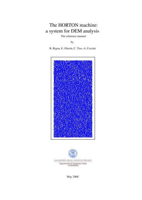
The HORTON machine:
a system for DEM analysis
The reference manual
by
R. Rigon, E. Ghesla, C. Tiso, A. Cozzini
May 2006

Cover image: Scheidegger 1967, Scheidegger’s network, created by Riccardo Rigon with Matematica c○
ISBN 10: 88-8443-147-6
ISBN 13: 978-88-8443-147-9

Readme!
This ebook was written by Riccardo Rigon and his collaborators (Università degli Studi di Trento, Di-
partimento di Ingegneria Civile e Ambientale).
free:
It is distribute along the license CREATIVE COMMONS deed: Attribution - No Derives 2.5 You are
• to copy, distribute, display, and perform the work
• to make commercial use of the work
Under the following conditions:
• Attribution. You must attribute the work in the manner specified by the author or licensor.
• No Derivative Works. You may not alter, transform, or build upon this work.
• For any reuse or distribution, you must make clear to others the license terms of this work.
• Any of these conditions can be waived if you get permission from the copyright holder.
Your fair use and other rights are in no way affected by the above. This is a human-readable summary
of the Legal Code (the full license): http://creativecommons.org/licenses/by-nd/2.5/legalcode

Contents
Contributions 1
1 Geomorphometry 5
2 DEM manipulation 7
2.1 MARK OUTLETS (h.markoutlets) . . . . . . . . . . . . . . . . . . . . . . . . . . . . . . . 10
2.2 PITSFILLER (h.pitfiller) . . . . . . . . . . . . . . . . . . . . . . . . . . . . . . . . . . . . 11
2.3 SPLIT SUBBASIN (h.splitsubbasin) . . . . . . . . . . . . . . . . . . . . . . . . . . . . . . 13
2.4 WATEROUTLET (h.wateroutlet) . . . . . . . . . . . . . . . . . . . . . . . . . . . . . . . . 15
3 The basic topographic attributes 17
3.1 Primary topographic attributes . . . . . . . . . . . . . . . . . . . . . . . . . . . . . . . . . 17
3.1.1 Gradients, Slopes, and Aspect . . . . . . . . . . . . . . . . . . . . . . . . . . . . . 17
3.1.2 Curvature and Laplace operator . . . . . . . . . . . . . . . . . . . . . . . . . . . . 19
3.2 Main derived topographic properties . . . . . . . . . . . . . . . . . . . . . . . . . . . . . . 20
3.2.1 Drainage directions
after [55] . . . . . . . . . . . . . . . . . . . . . . . . . . . . . . . . . . . . . . . . 20
3.2.2 Upslope catchment areas . . . . . . . . . . . . . . . . . . . . . . . . . . . . . . . . 24
3.3 Ab (h.Ab) . . . . . . . . . . . . . . . . . . . . . . . . . . . . . . . . . . . . . . . . . . . . 27
3.4 ASPECT (h.aspect) . . . . . . . . . . . . . . . . . . . . . . . . . . . . . . . . . . . . . . . 31
3.5 CURVATURES (h.curvatures) . . . . . . . . . . . . . . . . . . . . . . . . . . . . . . . . . 33
3.6 DRAINDIR (h.draindir) . . . . . . . . . . . . . . . . . . . . . . . . . . . . . . . . . . . . 35
3.7 FLOW DIRECTIONS
(h.flowdirections) . . . . . . . . . . . . . . . . . . . . . . . . . . . . . . . . . . . . . . . . 38
3.8 GRADIENTS (h.gradient) . . . . . . . . . . . . . . . . . . . . . . . . . . . . . . . . . . . 40
3.9 MULTITCA (h.multitca) . . . . . . . . . . . . . . . . . . . . . . . . . . . . . . . . . . . . 42
3.10 NABLA (h.nabla) . . . . . . . . . . . . . . . . . . . . . . . . . . . . . . . . . . . . . . . . 44
3.11 SLOPE (h.slope) . . . . . . . . . . . . . . . . . . . . . . . . . . . . . . . . . . . . . . . . 47
i

Contents
3.12 TOTAL CONTRIBUTING AREA
(h.tca) . . . . . . . . . . . . . . . . . . . . . . . . . . . . . . . . . . . . . . . . . . . . . . 49
3.13 TOTAL CONTRIBUTING AREA 3D
(h.tca3D) . . . . . . . . . . . . . . . . . . . . . . . . . . . . . . . . . . . . . . . . . . . . 51
4 Basin related analyses 53
4.1 DIAMETERS (h.diameters) . . . . . . . . . . . . . . . . . . . . . . . . . . . . . . . . . . 53
4.2 DIST EUCLIDEA (h.dist euclidea) . . . . . . . . . . . . . . . . . . . . . . . . . . . . . . 56
4.3 PRINCIPAL AXES (h.principal axes) . . . . . . . . . . . . . . . . . . . . . . . . . . . . . 58
4.4 MEAN DROP (h.mean drop) . . . . . . . . . . . . . . . . . . . . . . . . . . . . . . . . . 59
5 Network related measures 61
5.1 The Hack’s length and the Width function . . . . . . . . . . . . . . . . . . . . . . . . . . . 63
5.2 D2O (h.D2O) . . . . . . . . . . . . . . . . . . . . . . . . . . . . . . . . . . . . . . . . . . 64
5.3 D2O3D (h.D2O3D) . . . . . . . . . . . . . . . . . . . . . . . . . . . . . . . . . . . . . . . 66
5.4 DD (h.DD) . . . . . . . . . . . . . . . . . . . . . . . . . . . . . . . . . . . . . . . . . . . 68
5.5 EXTRACT NETWORK
(h.extractnetwork) . . . . . . . . . . . . . . . . . . . . . . . . . . . . . . . . . . . . . . . . 70
5.6 HACKLENGTHS (h.hacklength) . . . . . . . . . . . . . . . . . . . . . . . . . . . . . . . . 72
5.7 HACKLENGTH3D (h.hacklengths3D) . . . . . . . . . . . . . . . . . . . . . . . . . . . . . 74
5.8 HACKSTREAM (h.hackstream) . . . . . . . . . . . . . . . . . . . . . . . . . . . . . . . . 76
5.9 LANGBEIN (h.langbein) . . . . . . . . . . . . . . . . . . . . . . . . . . . . . . . . . . . . 78
5.10 MAGNITUDE (h.magnitudo) . . . . . . . . . . . . . . . . . . . . . . . . . . . . . . . . . 79
5.11 NET DIFF(h.netdif) . . . . . . . . . . . . . . . . . . . . . . . . . . . . . . . . . . . . . . 81
5.12 NETNUMBERING (h.netnumbering) . . . . . . . . . . . . . . . . . . . . . . . . . . . . . 83
5.13 RESCALED DISTANCE
(h.rescaleddistance) . . . . . . . . . . . . . . . . . . . . . . . . . . . . . . . . . . . . . . . 85
5.14 RESCALED DISTANCE 3D
(h.rescaleddistance3D) . . . . . . . . . . . . . . . . . . . . . . . . . . . . . . . . . . . . . 87
5.15 STRAHLER (h.strahler) . . . . . . . . . . . . . . . . . . . . . . . . . . . . . . . . . . . . 89
5.16 SEOL (h.seol) . . . . . . . . . . . . . . . . . . . . . . . . . . . . . . . . . . . . . . . . . . 91
6 Hillslope analisys 93
6.1 Definitions and main properties . . . . . . . . . . . . . . . . . . . . . . . . . . . . . . . . . 93
6.2 Hillslope2ChannelDistance
(h.h2cD) . . . . . . . . . . . . . . . . . . . . . . . . . . . . . . . . . . . . . . . . . . . . . 97
ii

6.3 Hillslope2ChannelDistance3D
Contents
(h.h2cD3d) . . . . . . . . . . . . . . . . . . . . . . . . . . . . . . . . . . . . . . . . . . . 99
6.4 Hillslope2ChannelAttribute
(h.h2cA) . . . . . . . . . . . . . . . . . . . . . . . . . . . . . . . . . . . . . . . . . . . . . 101
6.5 Classification and ordering . . . . . . . . . . . . . . . . . . . . . . . . . . . . . . . . . . . 103
6.6 GC (Geomorphic classes) (h.gc) . . . . . . . . . . . . . . . . . . . . . . . . . . . . . . . . 104
6.7 TC (TopographicClasses) (h.tc) . . . . . . . . . . . . . . . . . . . . . . . . . . . . . . . . . 108
7 Statistics 111
7.1 SUMDOWNSTREAM
(h.sumdownstream) . . . . . . . . . . . . . . . . . . . . . . . . . . . . . . . . . . . . . . . 111
7.2 COUPLEDFIELD MOMENTS
(h.cb) . . . . . . . . . . . . . . . . . . . . . . . . . . . . . . . . . . . . . . . . . . . . . . 113
8 Hydro-geomorphic Indexes and relations 115
8.1 TOPOGRAPHIC INDEX
(h.topindex) . . . . . . . . . . . . . . . . . . . . . . . . . . . . . . . . . . . . . . . . . . . 117
9 Geomorphology 119
9.1 TAU (h.tau) . . . . . . . . . . . . . . . . . . . . . . . . . . . . . . . . . . . . . . . . . . . 119
9.2 SHALSTAB (r.shalstab.ft) . . . . . . . . . . . . . . . . . . . . . . . . . . . . . . . . . . . 121
9.3 SOIL DEPTH (r.soil depht.ft) . . . . . . . . . . . . . . . . . . . . . . . . . . . . . . . . . 123
Appendix A 125
List of figures 127
Bibliografy 129
iii

Contents
iv

Contributions
Although the present handbook is edited by the authors listed, the applications presented are the product
of the work of some more people, here listed in chronological order: Riccardo Rigon, Paolo D’Odorico,
Paolo Verardo, Marco Pegoretti, Andrea Cozzini, Silvano Pisoni, Scott Overton, Andrea Antonello, Erica
Ghesla. The illustration of each application contains more details regarding specific contributions. Please
when using the Horton Machine, cite this manual and the original references listed in the text.

General information
The suite of HORTON programs is composed by a set of applications, i.e. a set of programs which carry
out some operations (on digital data of the terrain), and by the source code generating these applications. It
was developed by or under the supervision of Riccardo Rigon at the Department of Civil and Environmenta
Engineering of the University of Trento (ITALY). The programs are available according to the GPL (General
Public License) and can be found at (http://www.gnu.org/copyleft/gpl.html).
The code contained in HORTON, originally based on the fluidturtle C libraries, also available according
to the GPL, has been recently ported completely to Java and works inside the GIS JGRASS. The original
version of the routine is not anymore maintained since 2003.
The programs contained in HORTON generally use the RAM memory intensely. Although we try to
use the memory in a rational way (but not always), neither particular instruments nor particular codexes (to
improve, for example, the allocation of the matrix memory) have been optimized: this would have pushed
us dangerously far away from the purposes on which these libraries have been built, namely having the
geomorphology analysis instruments to use and modify easily. The main criterion for the Horton Programs
design has been the creation of an easily readable, modular and reusable code. The rest, also efficiency, is
subordinate.

To begin
The understanding of some basic elements of the GIS JGrass is necessary in order to use the Horton
Machine: you will find a complete description in the JgrassManual which is downloadable at the site
http://www.hydrologis.com.
A basic knowledge of geomorphometry is also needed. However, a minimal explanation of the contents
of the single chapters is provided at the beginning, whereas next chapter briefly introduces the topics. A
comprehensive introduction to geomorphometry literature, yet to be completed with [65], and related work,
is [57].
The following chapter 1 contains a very brief introduction to geomorphometry.
Chapter 2 contains the basic tools for DEM manipulation; chapter 3 the analysis of slopes, gradients,
curvatures, contributing areas and drainage directions; chapter 4 various tools from Riccardo Rigon research;
chapter 5, classic and less classic classification of river networks; chapter 6 some tools for hillslope metric
analysis (length, drainage density and so on), chapter 7 some tools for geometric characterization based on
the geometry of sites; chapter 8 deals with some tools prepared for the statistical analysis of the geomorphic
properties; in chapter 9 some geomorpic and hydrologic indexes are described. Finally, some tools for
hillslope stability and soild depth are presented.
JGRASS as well as The Horton Machine inherits the FluidTurtle file format which is explained in the
Appendix A.

For each application in the Horton machine a brief description is given according to scheme here after
presented.
HERE THE PROGRAM NAME
Description: it contains a brief description of what the program does.
Author and date: the author of the source code and of the following modifiers.
Inputs: It describes the data requested by the program in input. This data are contained in a file (the file
called ’nome’ is given as an example). If data are provided also interactively, this are specified with
enumeration. The example files contain comments concerning their contents. As a rule, the Horton
application code contains a ”main( )” executing all the I/O operations and a routine which, operating
on matrixes and vectors, executes the calculus; indications regarding the matrix content can be found
also in the comments of the source code.
Returns: Dealing with an application, generally the content of the output file is specified. Instead, if it were
a routine, we would deal with data and control values.
JGRASS Command: the syntax of the command given on the command line.
Notes: Notes about the program. Specially concerning its limitations (no code is perfect!) or the algorythms
used within the routine. A wish-list for the future versions and/or other information.
References: Articles or books which have inspired the codex or justified its necessity. Users are encouraged
to cite these papers in their own work.
Sources: All the sources necessary to the codex compilation, except for the basis routines (specified in the
appendixes). A more detailed documentation about the codex can be found in the source files and can
be extracted with doxygen.

1 Geomorphometry
The purpose of this analysis is to describe some quantitative instruments for understanding the morphol-
ogy of catchments. Indeed, the object of geomorphometry is characterizing quantitatively the morphology
of the Earth’s surface, and of the topographical properties of the basins, in order to device some indicators
of hydrologic and erosive processes and some instruments for a correct parametrization of the hydrologic
simulation models.
In the recent past and in the traditional geomorphologic practice, the characters of topography were derived
through field investigations and aerial photos; the morphology of topographic surfaces was synthetized in
some shape parameters and the channel network was described according to either Sthraler’s or Horton’s
schemes [65]. Now, the availability of digital elevation models (DEM) has irreversibly changed the analysis
of mountain geomorphology, and above all of the geomorphology at basin scale. Indeed, it has made it
possible to shift from a substantial lack to an abundance of data and from manual processing to automatic
analysis, starting from Moore’s works (for a complete bibliography see Wilson and Gallant, 2000 [13]),
Tarboton et al. [1989] [75], Jenson and Domingue [1988] [67], Jenson [1991] [70], Band [1993a] [7],
Montgomery and Foufula-Georgiou [48], Costa Cabral e Burges [1994] [41], Garbrecht and Martz [1997]
[18]. Nowadays the automatic analysis of topography enables to obtain reliable results and to estimante
a lot of quantitative information. Some issues, like the determination of the beginning of the channel in-
cision, still remain open. Moreover, although the traditional methodologies for technological reason can
work only with synthesis parameters [Abrahams, 1984 [1]], the modern analysis, supported by the use of
Geographic Information Systems (GIS), can easily deal with distributions of the same parameters and can
also inquire directly into many quantities once inaccessible to geomorphologues [Rinaldo et al., 1998 [4];
Rodriguez-Iturbe and Rinaldo, 1997 [65]], i.e. the mean length of a basin hillslopes [D’Odorico and Rigon]
[11]. The relations existing between some classical geomorphologic indicators, like for instance Horton’s
and Sthraler’s numbers and the distributed quantities are analyzed by [68] and [69] .
In this report we analyse the statistic properties of the elementary (or primary) topographic quantities of
the sample basins chosen for this convention.
The topographic properties analyzed by The Horton Machine can be distinguished in:
• primary topographic attributes (elevations, slopes and curvatures)
• main derived properties (contributing areas and drainage lengths)

1. Geomorphometry
• hydro-morphological indexes and curves (topographic index, proxies of the bottom shear stress gen-
erate by surface water flow and distance from the network and from the outlet)
The cartography and the distribution and probability curves of all primary quantities are here after reported.
As an example, the Flanginec river in Trentino (ITALY) is used. The original map was obtained by
coarse graining a LIDAR data set to a raster of 5 m side and is available with JGRASS.
6

2 DEM manipulation
Figure 2.1: Models for structuring a network of raster elevation data: (a) squared network obtained by moving a submatrix 3 × 3
centered on the nodes; (b) triangulated irregular network-TIN; (c) network based on the contour lines. The contour lines can be
used afterwards to subdivide the area in irregular polygons together with the lines of maximum slope (which constitute the envelope
of gradients) orthogonal to them [Moore and Grayson, 1990, Palacios and Cuevas, 1989; Moore, 1988; Moore and Grayson, 1989,
1990].
Topography is conceived by a bivariate continuous function
and with continuous derivative up to the second order almost everywhere.
z = f(x, y) (2.1)
The representation of the data, on a regular rectangular grid, constitutes undoubtedly the most common
and most efficient way in which the terrain digital data can be divided. Their direct treatment though can
produce some problems in the determination of very strong elevation changes, and in the treatment of the
flows in the diverging zones, which will be later discussed. The data presented in this raster, can be stored
in different ways, but the most efficient is the report of the vertical coordinate z for a subsequent series of
points along a given regular spacing profile. The elementary area is the one composed by four adjacent
points (three in the case of a regular grid) and consequentely the surface is discretized in elements (pixels)
centered in the grid nodes to which is attributed an elevation equal to their barycenter or, according to the
cases, to the mean elevation of the area. In other words, the elevation field constitutes a matrix of m × n
elements, each being the elevation of the point considered.
The minimum scale, i.e. the pixel size necessary for a correct representation of the terrain from the hy-
drologic point of view, depends on the ongoing morphologic processes. Normally pixels with a 10-m-long
side are assumed to be sufficient to identify most geomorphologic indicators [Montgomery and Foufola-
Geourgiou, 1993] however a finer resolution should be considered when available. However depending on

2. DEM manipulation
the processes studied, the problem is to know the procedure which produced the DEM from traditional topo-
graphic measures or other sources. The correct reproduction of second order derivatives (i.e. of curvatures),
which are the mirror of the physical processes acting, has to be considered.
The representation of a typical mountain topography from a DEM is depicted in Figure 2.2. Figure 2.3
shows the statistics of the same dataset as probability of exceedence of a given height. Also other statistics,
like the hypsographic curves, are often used in geomorphology (e.g. - [43], pp 211).
Figure 2.2: Topography of Flanginec basin
8

2. DEM manipulation
Figure 2.3: Statistics of the elevations of river Flanginec. For each elevation value the portion of area with highest elevation can
be read in ordinate
9

2. DEM manipulation
2.1 MARK OUTLETS (h.markoutlets)
description: It ”marks” the basin outlets with conventional number 10. In fact some applications in HOR-
TON request that the outlets are specified explicitly.
Author and date: Andrea Antonello, Andrea Cozzini, Silvia Franceschi, Erica Ghesla, Silvano Pisoni,
2005, Riccardo Rigon, 1998
Inputs:
1. file containing the matrix of the drainage directions to modify (obtained with flowdirections or
Output:
draindir);
1. file containing the matrix of the data assigned in input with the outlets set equal to 10;
JGRASS Command: h.markoutlets [–quiet] [–verbose] [–version] [–usage] –flow –inmapset
[–inputformat ] –mflow –mflowmapset [–mflowformat
] [–usegui]
Notes: It follows the drainage directions until it finds a value greater than 8. Then it marks the point directly
upriver as outlet.
Sources: h markoutlets.java
10

2.2 PITSFILLER (h.pitfiller)
2. DEM manipulation
Description: It fills the depression points contained in a DEM so that the drainage directions are defined in
each point. See, for instance [7] for a discussion of this and related issues.
Author and date: Andrea Antonello, Andrea Cozzini, Silvia Franceschi, Erica Ghesla, Silvano Pisoni,
2005, M. Pegoretti, Paolo Verardo & Riccardo Rigon, 1998.
Inputs:
1. the file containing the elevations;
Output:
1. matrix of the correct elevations;
JGRASS Command: h.pitfiller [–quiet] [–verbose] [–version] [–usage] –elevation –inmapset
[–inputformat ] –pit –outmapset [–outputformat
] [–usegui]
Notes: The flooding algorythm (pitsfiller) fills all pits present in the DEM. Obviously these could also be
real pits and not a product of the landscape gridding. In this case we should find a representation of
the drainage directions considering also the possible lakes and ponds, which is not yet implemented
References: [75] [56]
Sources: h pitfiller.java
See Also: DrainageDirections
11

2. DEM manipulation
Figure 2.4: The map of elevations without pit, calculated on the Flanginec river basin.
12

2.3 SPLIT SUBBASIN (h.splitsubbasin)
2. DEM manipulation
Description: A tool for labeling the subbasins of a basin. Given the Hack’s number of the channel network,
the subbasin up to a selected order are labeled. As shown in Figure 2.6 where Hack order 2 was
selected, the subbasins of Hack order 1 and 2 and the network of the same order are extracted
Author and date: Erica Ghesla, & Riccardo Rigon, 2005
Inputs:
1. the file containing the drainage directions (obtained with markoutlets);
2. the file of the order according the Hack lengths;
3. the file containing the contributing area (obtained with draindir or tca);
4. the threshold value for the contributing area;
5. the hackstream order file;
Output:
1. the file containing the net with the streams numerated;
2. the file containing the subbasins.
JGRASS Command: h.splitsubbasin [–quiet] [–verbose] [–version] [–usage] –flow –flowmapset
[–flowformat ] –hackstream –hackstreammapset

2. DEM manipulation
Figure 2.5: The subbasins calculated on the Flanginec river basin. Hachstream = 2.
14

2.4 WATEROUTLET (h.wateroutlet)
2. DEM manipulation
Description: Generates a watershed basin mask from a drainage direction map and a set of coordinates
representing the outlet point of watershed.
Author and date: Andrea Antonello, Andrea Cozzini, Silvia Francesch, Erica Ghesla, Silvano Pisoni, Ric-
cardo Rigon. Originally by Charles Ehlschlaeger, U.S. Army Construction Engineering Research
Laboratory.
Inputs:
1. the map containing the drainage directions (obtained with markoutlets);
2. the coordinates of the water outlet;
3. the map containing the channel network (obtained with extractnetwork);
Output:
1. he basin extracted mask;
2. a chosen map cut at the basin mask (the name assigned is input.mask).
JGRASS Command: h.wateroutlet [–quiet] [–verbose] [–version] [–usage] –drainage –basin
–northing –easting [–extractmap ] [–usegui]
Notes: The most important thing in this module is to choose a good water outlet. If the coordinates are
unknown, clic with the mouse on the network map.
References: This manual.
Sources: h wateroutlet.java
See Also: FlowDirections
15

2. DEM manipulation
Figure 2.6: The map containing the basin.
16

3 The basic topographic attributes
The primary topographic attributes are:
• aspect;
• slopes and gradient;
• Laplace operator;
• longitudinal, trasversal and normal curvatures;
The main derived quantities are:
• up-slope catchment areas;
• drainage directions.
3.1 Primary topographic attributes
3.1.1 Gradients, Slopes, and Aspect
The slope distribution is relevant from many points of view. Since the main motive-power of the hydro-
logic flows on the Earth’s surface and in the soil directly below is gravity, the surface gradient identifies,
in first approximation, the water flow directions and contributes to the determination of their speed. The
sub-surface flow is proportional to slope; the surface runoff to the root of the slope. Also the erosion and
the consequent solid transport depend on the gradients of the topographic surfaces: these have components
which are proportional to the gradients both in a linear and in a non-linear way [e.g. [12]]; moreover, zones
with a great slope are generally devoid of soil and they represent zones of exposed rock.
Indicating with:
fx = ∂z
∂x
fy = ∂z
∂y
(3.1)

3. The basic topographic attributes
and:
• The gradient is:
• the maximum-slope (the slope) angle is:
p = f 2 x + f 2 y
• and the aspect (measured counterclockwise from the ”x” axis) is:
(3.2)
∇z = (fx, fy) (3.3)
γ = arctan √ p (3.4)
α = arctan fy
From slopes, we deduce the drainage directions which correspond (up to inertial effects negligible at first
approximation) to the water flows.
fx
Figure 3.1: The slope of Flanginec basin
The flow directions are determined in the direction of maximum slope yet, in practice, the possible
drainage directions are limited to the discretization adopted in order to represent the real data. Indeed, each
pixel is surrounded by a set of other points, four, six or eight, according to the fine topologic structure chosen
and each represented in Figure (3.2).
18
(3.5)

3. The basic topographic attributes
Figure 3.2: Diagram of the possible topologies of river basin discretization: (a) isotropic hexagonal structure; (b) isotropic squared
four-direction structure; (c) eight-direction squared structure (isotropic or not, depending on how the diagonal directions are
weighted, i.e. topologically or geometrically)
Since the terrain digital data used by the programs described in this manual are provided on the basis
of matrixes whose elements (the pixels) are squared, during the present work the eight-direction topology
is normally adopted. Such choice makes it possible to discriminate sufficiently among the various direc-
tions, with no need to use a continuous representation of the surface, even if the limitation entails some
compromises [[55] and references therein]. The aspect is then often substituted by numbers (from 1 to 8) as
represented in Figure (3.2c).
3.1.2 Curvature and Laplace operator
The curvatures represent the deviations of the gradient vector for unit length (in radiants) along particular
curves plotted on the surface under consideration. In particular, the presence of non-zero curvatures has
relevant effects on the representation of the properties of the surfaces discretized. For example, if the surface
has a negative normal curvature, then the gradients have diverging directions at the extremes of the pixel,
P , and the contributing area in P is spread over several adjacent pixels: in this case topography is called
locally divergent. Vice versa, the surface is locally converging (negative curvature) and the contributing
area in P tends to be spread over a limited set of adjacent pixels and almost centainly on a single pixel.
19

3. The basic topographic attributes
Roughly speaking, the convex zones are hillslope zones, the concave zones are valleys. As it is known, the
latter contain the channel network. Then, the curvature tends to discriminate the points across the basin with
greater humidity content (the concave ones). This fact has relevant consequences on the overall hydrologic
behavior of basins and, in particular, on the production of runoff and on the evapotranspiration distribution.
The Laplace operator, which here represents the curvature, is defined by:
∇ 2 z = ∂2 2
z
∂x
+ ∂2 2
z
∂y
and it makes it possible to distinguish the convex zones (∇ 2 z < 0) from concave zones (∇ 2 z > 0) or
planar zones (∇ 2 z ∼ 0). Although, from a geometric differential point of view, it is possible to determine
a classification of topography, based on the combination of curvatures (see TC and GC), a simpler partition
of the landscape can based on the Laplace operator. Indeed, the terrain digital data produced with the
traditional techniques, do not return really reliable values of the curvature; on the contrary, the sign of the
Laplace operator is instead sufficiently correct.
3.2 Main derived topographic properties
3.2.1 Drainage directions
after [55]
The basic operation that must be carried out when processing DEM data is the determination of drainage
directions. This operation has important implications on the calculation of drainage areas and other quanti-
ties required for the description of a drainage system [e.g. [6], [39]]. The earliest and simplest method for
specifying drainage directions is to assign a pointer drom each DEM cell to one of its eight neighbors, either
adjacent or diagonal in the direction of the steepest downward slope. This method was introduced by [54]
and [44] and is commonly known as D8 (eight drainage directions). The D8 approach is characterized by
two major restrictions: (1) the drainage direction from each cell is restricted to eight possibilities, separated
by θ = π/4 rad (square cells are used: see also [15];[58], [41]) and (2) drainage area (see below) which
orignates over a two dimensional cell is treated as a point-source (nondimensional) and is projected downs-
lope by a line (one dimensional) [50]. To overcome these two restrictions different alternative methods have
been developed [55] but in the Horton Machine only variations on D8 method has been fully implemented
so far.
20
(3.6)

3. The basic topographic attributes
According to D8, a river basin is well defined from the numeric point of view if any point across the basin
except for the basin closure, has a lower point around itself. The points belonging to lakes or ponds and the
natural depressions constitute exceptions to this situation. The lakes are identified in the DEM in advance
(since they constitute a connected set of points of which the elevation -constant- and the location of one
point at least are known), while the smaller depressions are filled artificially until they identify a drainage
direction [[75]; [56]]. Problems can be given also by flat areas where no clear gradient is presented. [18]
suggested a method to overcome these situations.
Defining the drainage directions causes each pixel to be connected to the outlet and each pixel to be
an ”upriver” basin outlet univocally defined. According to the criterion of maximum slope, every element
drains towards the lowest element nearby. This usually does not coincide with the direction of the gradient
and a new method to minimize this deviation was proposed in [55]. In case the sites are distinguished with
indexes on the basis of a pre-established numeration, it is possible to express the drainage directions through
a matrix W , whose element is Wij, defined by the relation:
and also:
Wij =
being nn(i) the set of the elements surrounding i.
A correction to the D8 method
�
1 if j drains in i
0 otherwise
(3.7)
Wij = 1 se zj = min{zk k ∈ nn(i)} (3.8)
Using the ”pure” D8 method for the drainage direction estimation causes an effect of deviation from
the real direction identified by the gradients. Some authors, e.g. [15], claim that, in nature, there is also a
dispersive effect due to the subgrid variation of the gradients along the finite size of pixels, but this effect is
usually negligible in most of the real cases.
[16] chose the drainage direction according to the following scheme. Being
ei (i = 0, 1, 2, ...) (3.9)
the vector containing the elevation of the eight pixels surrounding one given pixel, and
di (i = 0, 1, 2, ...) (3.10)
the vector containing the pixel distances (greater for the pixel in the corner directions). The above situation
is shown in figure 3.3. Joining the eight neighbors with the central pixels, eight triangle are created and
21

3. The basic topographic attributes
the gradient vector is inside one of them. The gradient vector deviates from the side of the triangle which
represent two choices (p1 and p2) for a possible direction in the traditional D8 method. The Tarboton’s
method chose the direction among the two which is closer the the real gradient direction.
Figure 3.3: The drainage directions represented with reference to a generic pixel, i, indicated here with “0”. In red, is shown the
gradient direction, in blue are the eight surrounding triangles, in green a linear estimation of the deviation of the gradient from the
side direction and in pink an angular estimation of the same quantity.
For each triangle the slope of the sides s1 and s2 is:
s1 = e0 − e1
d1
s2 = e1 − e2
d2
The aspect of the gradient (i.e. its angular orientation), r,and its modulus, smax are:
r = arctan
smax =
� �
s2
s1
�
s 2 1 + s 2 �1/2 1
(3.11)
(3.12)
(3.13)
(3.14)
The deviation of the sides from the gradient can be expressed in two ways as in [55]. We can consider
the angle between the aspect and the sides (α1 and α2 in figure 3.3) or the distance between the center of
22

3. The basic topographic attributes
the pixel and the line along the gradients (δ1 and δ2 in figure 3.3). The first criterion implemented, D8-
LAD (least angular deviation), minimize the total angular deviation, the second criterion, D8-LTD (least
trasversal deviation), minimizes the total deviation length. The angular deviations are:
α2 = arctan
α1 = r (3.15)
� d2
The chosen direction is p1 if α1 ≤ α2 or the diagonal p2 if α1 > α2.
The transversal deviation are:
δ2 =
d1
δ1 = d1 sin α1
�
d 2 1 + d 2 �1/2 1 sin α2
�
− r (3.16)
(3.17)
(3.18)
In the D8-LAD method, the direction p1 is chosen of δ1 ≤ δ2 or p2 is chosen otherwise. Both the method
gives a drainage direction for any DEM cell. Besides, they can provide the estimation of the total deviation
from the gradients, just cumulating the angular or the linear deviation going from the higher pixel downhill.
The core of the new method is to to redirect the D8 drainage direction if use the total deviation (either
angular or linear) is larger than an assigned threshold value. For the k pixel, deviation are:
with
The cumulative total deviations are:
δ2(k) =
δ1(k) = d1 sin α1
�
d 2 1 + d 2 �1/2 1 sin α2
(3.19)
(3.20)
δ + 1 (k) = σδ1(k) + λδ + (k − 1) (3.21)
δ + 2 (k) = −σδ2(k) + λδ + (k − 1) (3.22)
where σ is the sign given to any direction and λ is a factor which the user can choose between 0 and 1.
As an example, the drainage direction is chosen to minimize: Lδ + (k) where k = 1, 2, .... If δ + 1
δ + 2 (k), is δ+ (k) = δ + 1
(k) e p = p1;
Otherwise, if δ + 1 (k) > δ+ 2 (k), is δ+ (k) = δ + 2
(k) e p = p2.
The other method, D8-LAD, utilizes the same procedure.
(k) ≤
If λ=0 the deviation’s counter has no memory and the pixel up-hill do not influence the choice. If λ=1 the
total deviation is entirely recorded. For the D8-LAD λ=0 is equivalent to use the steepest descent method.
23

3. The basic topographic attributes
Figure 3.4: How to assign the (σ) to the eight trangles (in blue). As above, in red, is the gradient, dash lines delimit the eight
triangles, in green is the linear deviation and in pink the angular deviation.
3.2.2 Upslope catchment areas
The upslope catchment (or simply contributing) areas represent the planar projection of the areas afferent
to a point in the basin. Once the drainage directions have been defined, it is possible to calculate, for each
site, the total drainage area afferent to it, indicated as TCA (Total Contributing Area). The number of sites
draining in the i-esimal element determines the total area Ai which can be expressed as follows:
Ai = �
j ∈ nn(i)
WijAj + Ri
(3.23)
where nn(i) represents the set of the eight (six, four or three) pixels surrounding the i-esimal site; Ri is
the area of every pixel. The use of the method of the maximum slope, with no partition of the flow coming
out from every pixel, makes the TCA an increasing function of the abscissa measured along any path from
upriver downhill. The discretized representation of the surfaces implies two principal problems: the first
(and more important) one is due to a topologic limitation, i.e. to the fact that we are able to consider a
limited number of drainage directions (for example in topology D4 there are 4 directions, with a spacing of
90 degrees: North, East, South, West; in topology D8, 8 directions, with a spacing of 45 degrees: North,
24

3. The basic topographic attributes
North-West, East, South-East, South, South-West, West, North-West); the second is bound to the gradient
variation in convex zones (with diverging gradient). The limitation of the possible directions entails that
surfaces oriented differently, (for example in direction 22 degrees) are bad represented, and systematic
deviations from the direction of the real flow can generate. The second problem is particularly relevant
for hillslope or conoid zones. As already described, where the curvature is positive, the gradient (and the
flows along with it) ”converges” towards a point; in the negative-curvature points, the gradient, at the pixel
extremes, points to different directions: then it tends to spread the flow on several adjacent pixels. Many
techniques have been implemented to compensate for these limitations in the procedures. A group of these
techniques consists in distributing the flow not in only one direction, but in many directions (multiple flow
directions) [15]
If we adopt a multiple flow direction criterion, the matrix W does not contain only one value differ-
ent from zero (and equal to one), but it can present several pixels with drained value different from zero,
provided that the sum of the contributions due to a pixel on all its neighbors is unitary. In this case:
�
α ≤ 1 se j drains in i
Wij =
0 otherwise
with:
(3.24)
�
Wij = 1 (3.25)
j
The partition is usually done considering that the nearby most lowered site is that receiving most of the flow,
followed by the second most lowered site and so on up to the last one, which appears as the one of greatest
elevation. In formal terms:
△hi
Wi,j = �
j ∈ pp(i) △hi
where pp(i) represents the set of the close sites with a lesser elevation than the i-esimal element.
(3.26)
The total cumulative area is an extremely important quantity in the geomorphologic and hydrologic study
of a river basin: indeed, it seems to be strictly related to the discharge flowing into the different points of the
system in uniform precipitation conditions.
Recent studies [65] have shown that the contributing areas distribute according to a power low:
P [A > a] ∼ a −β f(a/AT ) (3.27)
where AT is the area of the basin. Generally, the exponent of the probability curve is close to about β =
−0.43. The the power law deviation for small areas is due to the transition between hillslopes and channeled
zones. In big areas, there are not enough sample points and the distribution tends quickly to zero (because
of finite size). The function f in fact is:
lim
a→0 f(a/At) = 1 (3.28)
lim f(a/At) = 0
a→AT
25

3. The basic topographic attributes
Figure 3.5: Graphical elaboration of the contributing areas considering the flow according to the maximum-slope method referred
to Flanginec basin.
26

3.3 Ab (h.Ab)
3. The basic topographic attributes
Description: It calculates the draining area per length unit (A/b), where A is the total upstream area and b
is the length of the contour line which is assumed as drained by the A area see fig. 3.6. The contour
length is here be estimated by a a novel method based on curvatures.
Author and date: Erica Ghesla & Riccardo Rigon, 2004
Inputs:
1. the file containing the matrix of planar curvatures (obtained with curvatures);
2. the matrix with the total contributing areas (obtained with draindir or tca);
Output:
1. the file containing the matrix of the areas per length unit, A/b;
2. the file containing the matrix of the contour line, b.
h.aspect [–quiet] [–verbose] [–version] [–usage] –plan curv
–plan curvmapset [–plan curvformat ] –tca –tcamapset
[–tcaformat ] –alung
–alungmapset –alungformat –b –bmapset
[–bformat ] [–usegui]
Note: The drainage length, b is here evaluated in each point of the basin according to the value of the planar
curvature. The contour line is locally approximated by an arc having the radius inversely proportional
to the local planar curvature. It is in fact the curvature radius r is:
r = 1
kp
(3.29)
where kp is the planar curvature. Then, assuming that the contour line can be approximated by a circle
radius, it is also
t = αr t ′ = α(r − L) (3.30)
where t is the drained contour at the beginning (uphill) of the pixel and t ′ is the drained contour at the
end of the pixel (downhill), α is the angle enclosed between the two contours as an L is the pixel size,
as in figure 3.7.
L, in turn can be related to α as:
L = 2r sin
27
� �
α
2
(3.31)

3. The basic topographic attributes
and then:
Substituting 3.30 in 3.32 one obtain:
Finally, for every pixel, it is assumed:
where b is the drained contour.
� �
L
α = 2 arcsin
2r
(3.32)
� �
L
t = 2 arcsin r t
2r
′ � �
L
= 2 arcsin (r − L) (3.33)
2r
b ∼ t ′
(3.34)
To very convergent sites, there correspond a proportionally shrinking contour line, as in figure 3.7,
and to divergent site, as opposed to what shown in figure 3.7, an enlarging drainage line.
References: [51], this manual.
Sources: h Ab.java
See Also: TCA, CURVATURES, DRAINDIR.
28

Figure 3.6: The graphical description of the area A and the length of the contour line b.
Figure 3.7: The contour line in a pixel.
29
3. The basic topographic attributes

3. The basic topographic attributes
Figure 3.8: The areas per length unit of the basin of the Flanginec river.
Figure 3.9: The contour line of the basin of the Flanginec river.
30

3.4 ASPECT (h.aspect)
3. The basic topographic attributes
Description: It estimates the aspect (i.e. the inclination angle of the gradient) by considering a reference
system which puts the zero towards the east and the rotation angle anticlockwise. It differs from
the drainage directions in which it is given in radiants and it is a continuous function while drainage
direction returns a number between 1 and 10. In figure 3.10 is reported a pictorial view of the aspect
of the basin of Flanginec river. NODATA is a negative number. The aspect is 0 in the the South
direction and increase clockwise.
Author and date: Andrea Antonello, Silvia Franceschi, Erica Ghesla, Silvano Pisoni, 2005, Andrea Cozzini,
Riccardo Rigon, 2001
Inputs:
1. the file containing the matrix of the pitless elevations (as generated by the pitsfiller application);
Output:
1. the file containing the aspect matrix;
JGRASS command: h.aspect [–quiet] [–verbose] [–version] [–usage] –pit –pit –pitmapset
[–pitformat ] –aspect –outmapset [–outputformat
] [–usegui]
Note: Given the difficulty in defining the aspect on the matrix boundary, for the pixels belonging to this
we suppose that the direction angle of the gradient is turned, starting from the pixel centre, along the
maximum slope direction.
References: This manual
Sources: h aspect.java
See Also: Drainagedirections
31

3. The basic topographic attributes
Figure 3.10: The aspect of the basin of the Flanginec river.
32

3.5 CURVATURES (h.curvatures)
3. The basic topographic attributes
Description: It estimates the longitudinal (or profile), normal and planar curvatures for each site through a
finite difference schema. These are defined at the beginning of this chapter and estimated by a finite
difference method. The longitudinal curvature represent the deviation of the gradient along the the
flow (it is negative if the gradient increase), the normal and planar curvatures are locally proportional
and measure the convergence/divergence of the flow (the curvature is positive for convergent flow).
Some examples of this kind of geomorphological analysis are displayed in fig 3.11.
Author and date: Andrea Antonello, Silvia Franceschi, Erica Ghesla, Silvano Pisoni, 2004, Andrea Cozzini
& Riccardo Rigon, 1999
Inputs:
1. the file containing the matrix of elevations (obtained with pitfiller);
Output:
1. the file containing the matrix of longitudinal curvatures;
2. the file containing the matrix of normal (or tangent) curvatures;
3. the file containing the matrix of planar curvatures;
JGRASS Command: h.curvatures [–quiet] [–verbose] [–version] [–usage] –pit –pitmapset
[–pitformat ] –prof curv –prof curvmapset [–prof curvformat
] –plan curv –plan curvmapset [–plan curvformat
] –tang curv –tang curvmapset [–tang curvformat
] [–usegui]
Notes: The planar and normal (or tangent) curvatures are proportional to each other. To function, the
program uses a matrix in input with a NOVALUE boundary and as a rule it places the curve equal to
zero on the catchment boundary.
References: [50], [46]
Sources: h curvatures.java
33

3. The basic topographic attributes
Figure 3.11: The calculation of the planar curvature, the longitudinal (profile) curvature and the planar curvature of the basin of
the Flanginec river.
34

3.6 DRAINDIR (h.draindir)
3. The basic topographic attributes
Description: It calculates the drainage directions minimizing the deviation from the real flow. The devia-
tion is calculated using a triangular construction and it could be given in degrees (D8 LAD method) or
as trasversal distance (D8 LTD method). The deviation could be cumulated along the path using the
λ parameter, and when it assumes a limit value the flux is redirect toward the real gradient direction.
If the drainage network is known and marked in a raster matrix, its flow directions can be kept fixed.
Autthor and date: Andrea Antonello, Andrea Cozzini, Silvia Franceschi, Silvano Pisoni, 2005, Erica Gh-
esla, Riccardo Rigon, 2004.
Inputs:
1. the method to use: normal or net fixed
2. the file containing the matrix of elevations (obtained with pitfiller);
3. the file containing the old drainage direction matrix (obtained with flowdirections);
4. if we choose to fix the network, the map containing the drainage directions along the network;
5. the λ parameter (a value in the range 0 - 1);
6. the method choosen: LAD (angular deviation) and LTD (trasversal distance);
Output:
1. the file containing the new drainage directions;
2. the file containing the total contributing areas calculated with this drainage directions.
JGRASS Command: h.draindir [–quiet] [–verbose] [–version] [–usage] –pit –pitmapset

3. The basic topographic attributes
Sources: h draindir.java
See Also: PITFILLER, FOLWDIRECTIONS.
Figure 3.12: The new drainage directions of the basin of the Flanginec river.
36

3. The basic topographic attributes
Figure 3.13: The total contributing areas calculated with the new drainage directions. Flanginec river basin.
37

3. The basic topographic attributes
3.7 FLOW DIRECTIONS
(h.flowdirections)
Description: it calculates the drainage directions with the method of the maximal steepest descent slope,
choosing it among 8 possible directions, as specified in the opening of this chapter (after [16]).
Author and date: Andrea Antonello, Andrea Cozzini, Silvia Franceschi, Erica Ghesla, Silvano Pisoni,
2005, Riccardo Rigon, 1998
Inputs:
1. the file containing the matrix of elevations (obtained with pitfiller);
Output:
1. the file containing the matrix of the drainage directions;
JGRASS Command: h.flowdirections [–quiet] [–verbose] [–version] [–usage] –pit –pitmapset
[–pitformat ] –flow –flowmapset [–flowformat ]
[–usegui]
Notes: The maximal slope direction is chosen among the 8 possible directions and codified with numbers
ranging from 0 to 8 as specified in the first chapter of this handbook. Such method derives from the
one originarily used by D. Tarboton in his Phd thesis. However the outlets are marked with value 10.
The NODATA is 9 (beware: many other programs assume it)
References: [75],[65]
Sources: h flowdirections.java
See Also: Aspect
38

Figure 3.14: The flowdirections of the basin of the Flanginec river.
39
3. The basic topographic attributes

3. The basic topographic attributes
3.8 GRADIENTS (h.gradient)
Description: It estimates the gradient in each site, defined as the module of the gradient vector (see fig.
3.18)
Author and date: Andrea Antonello, Silvia Franceschi, Erica Ghesla, Silvano Pisoni, 2005, Andrea Cozzini
& Riccardo Rigon, 2000
Inputs:
1. description file containing the matrix of the elevations (obtained with pitfiller);
Output:
1. description file containing the matrix of the gradients;
JGRASS command: h.gradient [–quiet] [–verbose] [–version] [–usage] –pit –pitmapset
[–pitformat ] –gradient –gradientmapset [–gradientputformat
] [–usegui]
Notes: Let’s observe that gradients, contrarily to slope, does not use the draimage directions defined by
drainagedirections. Moreover, gradients calculates only the module of the gradient which in reality
is a vectorial quantity, oriented in the direction from the minimal to the maximal potential. As a rule,
the program places on the catchment boundary the gradient equal to zero.
References: [65], [39]
Sources: h gradient.java
See also: drainagedirections, slope, curvature
40

Figure 3.15: The gradient calculated on the basin of the river Flanginec.
41
3. The basic topographic attributes

3. The basic topographic attributes
3.9 MULTITCA (h.multitca)
Description: It calculates the contributing areas differently in convex and concave areas. In the first ones,
the flow of one pixel is subdivided over all the lower adjacent pixels; in the second ones instead only
one drainage direction is used. In our case, the weight used for the partition of the flow is inversely
proportional to the difference in elevation between the pixel and a downstream pixel normalized by
the total drop:
∆zij
Wij = �
j∈{i} ∆zij
(3.35)
where j ∈ {i} means that j spans all the points close to i and lower than it. ∆zij is the drop in
elevation between i and j.
Author and date: Andrea Antonello, Silvia Franceschi, Erica Ghesla, Silvano Pisoni, 2005, Andrea Cozzini
& Riccardo Rigon, 1999
Inputs:
1. file containing the matrix of elevations (obtained with pitfiller);
2. file containing the matrix of the drainage directions (obtained with markoutlets);
3. file containing the matrix of the aggregated topographic classes 9 (obtained with tc)
Output:
1. file containing the matrix of the contributing areas;
JGRASS Command: h.multitca [–quiet] [–verbose] [–version] [–usage] –pit –pitmapset

Figure 3.16: The map of multitca calculated on the basin of the river Flanginec.
43
3. The basic topographic attributes

3. The basic topographic attributes
3.10 NABLA (h.nabla)
Description: the program can work in two different ways:
1. It estimates, for each site, the Laplace operator of the quantity given in input, with a scheme at
the finite differences:
∇ 2 z = 1 [zi+1,j + zi−1,j − 2zi,j]
2 △y 2
+ 1 [zi,j+1 + zi,j−1 − 2zi,j]
2 △x 2
2. It subdivides the sites in three categories: planar, concave and convex, identifying the categories
through the Laplace operator. The planar sites are those for which ∇ 2 z ≤ ɛ, where ɛ is a prefixed
threshold value. The convention adopted in is the following:
• if |∇ 2 z| ≤ ɛ → 3 (planar sites)
• if |∇ 2 z| > ɛ → 1 (concave sites)
• if |∇ 2 z| < −ɛ → 2 (convex sites)
Author and date: Andrea Antonello, Andrea Cozzini, Silvia Franceschi, Erica Ghesla, Silvano Pisoni,
2005, P. Verardo. e R. Rigon, 1998
Inputs:
1. file containing the matrix of the drainage directions (obtained with markoutlets);
2. the choice between the calculation of the real value or of the classes
3. if we choose the second option, we must specify the threshold to define planarity.
Output:
1. file containing the matrix of the Laplace operator, or the topographic classes (see fig 3.10);
JGRASS Command: h.nabla [–quiet] [–verbose] [–version] [–usage] –pit –pitmapset
Notes:
[–pitformat ] –nabla –nablamapset [–nablaformat ]
–mode –th nabla [–usegui]
References: [65], [61]
Sources: h nabla.java
See Also: Curvature
44

Figure 3.17: The map of Laplance operetor calculated on the basin of the river Flanginec.
45
3. The basic topographic attributes

3. The basic topographic attributes
Figure 3.18: The topographic calculated classes on the basin of the river Flanginec.
46

3.11 SLOPE (h.slope)
3. The basic topographic attributes
Description: It estimates the slope in every site by employing the drainage directions. Differently from the
gradients, slope calculates the drop between each pixel and the adjacent points placed underneath and
it divides the result by the pixel length or by the length of the pixel diagonal, according to the cases.
The greatest value is the one chosen as slope.
Author and date: Erica Ghesla 2005, Andrea Cozzini & Riccardo Rigon, 1999
Inputs:
1. files containing the matrix of elevations (obtained with pitfiller);
2. files containing the matrix of the drainage directions (obtained with markoutlets);
Output:
1. matrix of the slopes;
JGRASS Command: h.slope [–quiet] [–ver>bose] [–version] [–usage] –pit –pitmapset
[–pitformat ] –flow –flowmapset [–flowformat ]
–slope [–slopemapset ] [–slopeformat ] [–usegui]
Notes: to estimate slopes, this program considers the drainage directions, estimating the slope of every
pixel in the direction of the less high, near pixel (steepestdescent). For many purposes, this slope is
used as an extimation of the gradient. The pattern shown in Figure 3.18 and 3.21 are in fact very
similar. However, it is apparent that the two definition do not coincide at al.
References: [65], [39], [75]
Sources: h slope.java.
See Also: gradients
47

3. The basic topographic attributes
Figure 3.19: The slope calculated on the basin of the river Flanginec.
48

3.12 TOTAL CONTRIBUTING AREA
(h.tca)
3. The basic topographic attributes
Description: The upslope catchment (or simply contributing) areas represent the planar projection of the
areas afferent to a point in the basin. Once the drainage directions have been defined, it is possible
to calculate, for each site, the total drainage area afferent to it, indicated as TCA (Total Contributing
Area).
Author and date: Andrea Antonello, Silvia Franceschi, Erica Ghesla, Silvano Pisoni, 2005, Andrea Cozzini
& Riccardo Rigon, 1999
Inputs:
1. the file containing the matrix of drainage directions (obtained with markoutlets);
Output:
1. the file containing the matrix of the real areas;
JGRASS Command: h.tca [–quiet] [–verbose] [–version] [–usage] –flow –flowmapset
[–flowformat ] –tca –tcamapset [–tcaformat ] [–
usegui]
References: [41], [65], [39], [75]
Notes:
Sources: h tca.java
See also: A/b section 3.3, TCA3D section 3.12, MULTITCA section 3.9.
49

3. The basic topographic attributes
Figure 3.20: The total contributing area calculated on the basin of the river Flanginec.
50

3.13 TOTAL CONTRIBUTING AREA 3D
(h.tca3D)
3. The basic topographic attributes
Description: It estimates the real draining area and not only its projection on the plane as the TCA do.
Author and date: Erica Ghesla, Riccardo Rigon, 2005.
Inputs:
1. the file containing the matrix of pitless elevations (obtained with pitfiller);
Output:
1. the file containing the matrix of the real areas;
JGRASS Command: h.tca3D [–quiet] [–verbose] [–version] [–usage] –pit –pitmapset
[–pitformat ] –flow –flowmapset [–flowformat ]
–tca3D –tca3Dmapset [–tca3Dformat ] [–usegui]
Notes: The way to calculate the 3D area is to approximate with triangles the DEM surface and then sum-
ming the triangles area going downstream from sources to outlet.
References: This manual
Sources: h tca3D.java
See also: TCA section 3.12.
51

3. The basic topographic attributes
Figure 3.21: The total contributing area 3D calculated on the basin of the river Flanginec.
52

4 Basin related analyses
This chapter deals with the delineation of a basin from a DEM and the extraction of some indicators
of the basin form or “shape parameters”. To some extent the exiting literature on the subject seems out of
date since it is clear that the need for ”indicators” reveals the inability to do real statistics on the basins.
Among the literature[5] is certainly a first reading which emphasizes that the search for such indicators is
also a search for the signatures of basin evolution and history. Very seldom the basins shape has been treated
in a separate manner from the channel networks, since the network “is the basins” (up to the point where
hillslope are) as the recent fractal theories of the river geomorphology state [65]. From DEM perspective the
river basin is obtained once the drainage directions are traced and the divides between two basins are those
points from which drainage directions diverge. As [81] points out drainage and divides are interlocked.
DEMs introduce some new problems but also let calculate shape indicators for any point inside a basin and
eventually to make statistics out of it.
A first set of ’new’ terrain measures includes mean elevation, [25], [78]. ’New’ parameters, however,
rarely are; many describe the same basic attribute of surface form and thus are redundant [57] and we keep
the simplest ones [52]. Fractal interpretation of surfaces added new fuel to some measurements even if
more attention has been given to the planar features of the basins (probably an inheritance of the “map,
pencil and sweat” times of geomorphometry) than to the more complicated problem of characterizing relief,
or Z-domain, attributes of continuous topography [35]. The property investigated in such fractal analysis is
the “self-affinity” whose meaning is discussed in [20] and is connected to the so-called Hack’s law which
however involves the definition of the channel network inside the basin.
4.1 DIAMETERS (h.diameters)
Description: It calculates the diameter of the basin subtended to a point. This is the distance between the
basin outlet and the point on the boundary farest from it. The calculus is repeated for each significant
point contained in a DEM. There could be alternative definitions of diameter (as for instance the

4. Basin related analyses
distance between any two points of a basin), here not considered.
Author and date: Erica Ghesla, 2005, Riccardo Rigon, 1998
Inputs:
1. the file containing the matrix of the drainage directions (obtained with markoutlets);
2. it is necessary to choose if in the calculus only the ’source’ points, or all points (as possible
Output:
points belonging to the sub-basins boundaries) have to be considered. This if effected by typing,
when requested, 1 or 0.
1. the file containing the matrix of the diameters;
JGRASS Command: h.diameters [–quiet] [–verbose] [–version] [–usage] –flow –flowmapset
[–flowmformat ] –diameters –diametersmapset [–
diametersformat ] –mode [–usegui]
Notes: Since the diameter is calculated for the basin subtended to every point, the computation is quite
slow.
References: [20]
Sources: h diameters.java
See Also: Hacklength, Hacklength3D, TopologicalDiameters,
54

Figure 4.1: Diameters calculated on the basin of the river Flanginec.
55
4. Basin related analyses

4. Basin related analyses
4.2 DIST EUCLIDEA (h.dist euclidea)
Description: It calculates the euclidean distance of each pixel from the outlet of the bigger basin which
contains it.
Author and date: Erica Ghesla, 2005, Andrea Cozzini & Riccardo Rigon, 2000
Inputs:
1. the file containing the matrix of the drainage directions (obtained with markoutlets);
Output:
1. the file containing the matrix of the distances;
item [JGRASS Command:] h.dist euclidea [–quiet] [–verbose] [–version] [–usage] –flow –
flowmapset [–flowmformat ] –dist euclidea –dist euclideamapset
[–dist euclideaformat ] [–usegui]
Notes: The program is a trivial application of the Pythagoras theorem formed by the plane Cartesian axes
with the line joining the pixel in question and the outlet.
References: [62]
Sources: h dist euclidea.java
56

Figure 4.2: The euclidean distance calculated on the basin of the river Flanginec.
57
4. Basin related analyses

4. Basin related analyses
4.3 PRINCIPAL AXES (h.principal axes)
Description: principal axes finds the main moments of inertia of each subnet of a channel net. The mo-
ments of inertia are defined as the moments of inertia with respect to the axes of a basin, considered
as a bidimensional body with uniform mass. The moments are first calculated with respect to the
coordinated axes. Then, the maximal ad minimal eigenvalues representing the moments of inertia
with respect to a particular couple of axes (the main axes exactly) are calculated. It is known that the
moment of inertia with respect to an arbitrary couple of axes is a symmetrical tensor which possesses
then (D 2 + D)/2 independent components, where (D = 2 in this case).
Author and date: Erica Ghesla, 2005, Riccardo Rigon, 1998
Inputs:
1. the map of the drainage directions (obtained with markoutlets);
2. the map of the contributing areas (obtained with draindir or tca);
Output:
1. the map containing the greater eigenvalue;
2. the map containing the lesser eigenvalue.
JGRASS command: h.principal axes [–quiet] [–verbose] [–version] [–usage] –flow –flowmapset
[–flowmformat ] –tca –tcamapset [–tcaformat
] –principal axes1
–principal axesmapset1 [–principal
axesformat1 ] –principal axes2 –principal axesmapset2
[–principal axesformat2
] [–usegui]
Notes: The application contains three main routines: baricenter, moment of inertia and principal axes,
which are documented in the following codex.
References: any text of elementary classic mechanics or [52]
Sources: h principal axes.java
58

4.4 MEAN DROP (h.mean drop)
4. Basin related analyses
Description: It calculates the mean value of a quantity defined by the input matrix (for example of eleva-
tions) calculated on the basin upriver with respect to every point, decreased of the value of the quantity
measured in the point itself (for instance the elevation of the point: from which the name). If B is the
quantity examined, then: L(j) = ( �
i Bi)j/Aj − Bj.
Author e date: Erica Ghesla, 2005, Marco Pegoretti e Riccardo Rigon, luglio 1999
Inputs:
1. the file of the drainage directions (obtained with markoutlets);
2. the file of the contributing areas (which, being the contributing areas measured in pixels, is
necessary to obtain the averaged value of the quantity);
3. the file containing the quantity of which estimating the mean value
Output:
1. the file containing the mean values of the quantity for each point within the basin ananyzed.
JGRASS Command: h.mean drop [–quiet] [–verbose] [–version] [–usage] –flow –flowmapset
Note:
[–flowmformat ] –tca –tcamapset [–tcaformat
] –summ
–summmapset [–summformat ] –mean drop –mean dropmapset
[–mean dropformat ] [–usegui]
References: This manual
Sources: h mean drop.java
59

4. Basin related analyses
Figure 4.3: The mean drop calculated on the basin of the river Flanginec.
60

5 Network related measures
The work on ridges and water courses dates back at least to the eighteenth century and almost from the
early beginning was linked to theory of evolution of river networks. From this point of view a very recent
contribution is given by [65]. A necessary introductory reading for the subject in study here is also [1]. [30]
collects a series of fundamental paper on the subject which includes [23], [45],[5];[53]; [36]; [37]; [38] and
other fundamental papers some of which will be cited later on and in [57]. Among the recent papers [20];
[4]; [68];[69] and references therein brings some new stuff and knowledge. All the above papers refers to
the branching structure on river basin (ultimately found to be a fractal) and to its classification or ordering.
However, once the network is delineated (or “extracted” as it is usually said) network informations can be
used to several goals. One of the main is to infer the hydrological response, either looking at the statistical
structure of the networks (e. g. - [66]; [21] ) or by the actual distribution of pathways called width function,
e.g. [65].
Figure 5.1: The network of the river Flanginec.

5. Network related measures
A river network is a (topologically) 1-D tree-like structure. Actually it is a oriented trifurcated tree since,
as shown in figure, the channels merge (usually) two by two in each node (or junction) and the flow through
the tree is given by the drainage directions (upstream to downstream). The outlet is the root of the tree. The
leaves of the tree are called sources. For what regards all the analysis in this chapter the channel are true 1-D
elements with no structure inside. In the past, based on the topological classification of the river networks,
a lot of science has been made [1], [65].
Strahler [53] introduced the following classification of river networks tree: i) sources are of order 1; ii)
when two stream of order 1 merge they form a stream of order 2; iii) in general when two streams, of order
i and j merge they continue into a stream of order which is max(i, j) if i �= j, otherwise they form a new
stream of order i + 1 = j + 1. Thus a stream is composed usually by many links.
A different labeling scheme for the network was introduced by Shreve [36] who numbered the links
according to the number of sources upstream. The numbers of each link was called the magnitude of the
link. The magnitude was used as a proxy for the contributing areas to each link.
Strahler ordering was used to express the so called Horton’s laws: :
The bifurcation law
N(ω, Ω)
N(ω + 1, Ω) ≈ RB (ω = 1, 2, .., Ω) (5.1)
where RB is said bifurcation ratio, Nω is the number of stream of order ω in a given river network, Ω is the
order of the network, i.e. the maximum Strahler’s order in the network. The length’s law
L(ω + 1, Ω)
L(ω, Ω) ≈ RL (ω = 1, 2, ..., Ω) (5.2)
where RL is said length ratio, Lω is the average lenght of stream of order ω in a given river network. and
the areas law (actually due to Schumm)
A(ω + 1, Ω)
A(ω, Ω) ≈ RA (ω = 1, 2, ...Ω) (5.3)
where RA is said area ratio, Aω is the average total area at the outlet of streams of order ω in a given river
network.
Eventually the Horton’s law where found to be the signature of the fractality of the river network and
related to power laws [65].
62

5.1 The Hack’s length and the Width function
5. Network related measures
The Hack’s length is the distance from any point in the basin to the divides, measured along the drainage
directions. Starting from a point, P an going uphill, at any bifurcation the stream with larger area is followed.
If two merging stream have the same contributing area, the longest is followed. Otherwise one of the
stream is chosen at random. The Hack length is the geomorphic signature of what the hydrologists call the
concentration time of the basin closed at P . As follows from [62], the distribution of Hack’s length inside a
large enough basin is approximated by a power law:
P [L > l] = l −γ g(l/LT ) (5.4)
where g is a scaling function, l the Hack’s length, LT a scale length. The exponent γ, is usually around -0.8
and is linked to other power law distributions [4].
If instead of the Hack’s length is considered the distance from any point, P , in a basin to the outlet (D2O)
of the basin (also measured along the drainage directions), one can derive the so called width function [33].
This is the probability density function of the above quantity and it is an indicator of “the width” of the
basin at a certain distance from the outlet. As shown in [11] and reference therein from this function can be
obtained a geomorphic instantaneous unit hydrograph. The model Peakflow, also implemented in JGRASS,
uses it.
63

5. Network related measures
5.2 D2O (h.D2O)
Figure 5.2: Hack’s distances from the devides referred to Flanginec basin.
Description: D2O (Distance to outlet) calculates the projection on the plane of the distance of each pixel
from the outlet, measured along the drainage directions. By aggregating the matrix so obtained, we
get the so called width function. The program can work in two different ways: it can calculate the
distance from the outlet either in pixel number (0:topological distance mode), or in meters (1:simple
distance mode).
Author and date: Andrea Antonello, Andrea Cozzini, Erica Ghesla, 2004, R. Rigon, 1998
Inputs:
1. the file containing the matrix of the drainage directions (obtained with markoutlets);
Output:
1. the file containing the matrix of the distances;
JGRASS Command: h.D2O [–quiet] [–verbose] [–version] [–usage] –flow –flowmapset
[–flowformat ] –dist2outlet
–dist2outletmapset [–dist2outletformat
] –mode [–usegui]
64

Figure 5.3: The topological distance to outlet calculated on the basin of the Flanginec.
5. Network related measures
Notes: The distance is estimated by following the path joining each pixel with the outlet following the
drainage directions. In the topological mode, the distance is measured in pixel number and without
distinguishing between directions parallel to the coordinates and diagonal directions. In the simple
mode, the distance is obtained in meters and oblique directions (D8 flow is assumed) are calculated
applying the Pithagorean theorem.
References: [11] and references therein, [34]
Sources: h D2O.java
See Also: drainagedirections, d2o3D
65

5. Network related measures
5.3 D2O3D (h.D2O3D)
Description: It calculates the distance of every pixel within the basin, considering also the vertical coordi-
nate (differently from distance2outlet which calculates its projection only)
Author and date: Erica Ghesla, 2005, R. Rigon, 1998
Inputs:
1. the file of elevations (obtained with pitfiller);
2. the file of the draining directions (obtained with markoutlets);
Output:
1. the file containing the distances.
JGRASS Command: h.D2O3D [–quiet] [–verbose] [–version] [–usage] –pit –pitmapset
Note:
[–pitformat ] –flow –flowmapset [–flowmformat ]
–dist2outlet
–dist2outletmapset [–dist2outletformat
] [–usegui]
References: This manual
Sources: h D2O3D.java
See Also: drainagedirections, D2O
66

Figure 5.4: The real 3-dimensional distance to outlet calculated on the basin of the Flanginec River.
67
5. Network related measures

5. Network related measures
5.4 DD (h.DD)
Description: It estimates the drainage density function for the basin upstream of each pixel. Drainage
density is defined as the total network length (i.e. the sum of all the stream lengths) divided by the
total length of the up-slope catchment area: Z/A. It has the the dimension of the inverse of a length
and such a length was shown by Horton to be an estimator of the average hillslope length.
Author and date: Erica Ghesla, 2005, Andrea Cozzini & Riccardo Rigon, 2001
Inputs:
1. the file containing the matrix of the hack distances (obtained with hacklength);
2. the file containign the channel network (obtained with extractnetwork);
3. the file containing the matrix of the upriver contributing areas (obtained with draindir or tca);
Output:
1. the file containing the matrix of the total distances of each point of the net from the outlet;
2. the file containing the matrix of the drainage density;
JGRASS Command: h.DD [–quiet] [–verbose] [–version] [–usage] –flow –flowmapset
[–flowmformat ] –tca –tcamapset [–tcaformat ] –
net –netmapset [–netformat ] –dd –ddmapset
[–ddformat ] [–usegui]
Notes: The distance of each pixel from the outlet is a simple application of the routine sum downstream.c
at the Hack distances estimated for each pixel, so the sum of this quantity effected only for the pixels
belonging to the net makes it possible to estimate the net length in each point.
References: [65]
Sources: h DD.java
See Also: tca, tca3D,
68

Figure 5.5: The drainage density calculated on the basin of the Flanginec.
69
5. Network related measures

5. Network related measures
5.5 EXTRACT NETWORK
(h.extractnetwork)
Description: It extracts the channel network from the drainage directions in five possible ways:
1. by using a threshold value on the contributing areas (then only the pixels with contributing area
greater than thethreshold are the channel heads) → mode 0;
2. by using a threshold value of the parameter: α∇ n z √ A, equivalent to a threshold value of the
stress tangential to the bottom → mode 1;
3. by using a threshold value on the stress tangential to the bottom → mode 2;
Individuated the beginning of the channel incision, the points upriver are considered as canalized.
Author and date: Andrea Antonello, Andrea Cozzini, Silvia Franceschi, Erica Ghesla, Silvano Pisoni,
2005, Riccardo Rigon, 1998
Inputs:
1. the file containing the matrix of the drainage directions (obtained with markoutlets);
2. the file containing the matrix of contributing areas (calculated with draindir, tca or multitca);
3. the methodology for extracting the net;
Output:
• if mode 0:
(a) other files are not requested
• if mode 1:
(a) the file containing the matrix of the slopes (calculated with slope);
• if mode 2:
(a) the file containing the matrix with the classes aggregated by GC;
1. the file containing the matrix which individuates the channel network;
JGRASS Command: h.extractnetwork [–quiet] [–verbose] [–version] [–usage] –prof curv –
prof curvmapset [–prof curvformat ] –tang curv
–tang curvmapset [–tang curvformat ]–cp3map
–cp3mapmapset [–cp3mapformat

Figure 5.6: The network of the river Flanginec extracted with a treshold on the TCA.
Notes: the matrix with the channel net individuates two classes of elements on the DEM:
• non-canalized sites (0);
• channel sites (2);
References: [32],[48] [17], [65],[49] [60], [47], [74]
See Also: TC, GC, FLOWDIRECTIONS, DRAINDIR, GRADIENT, SLOPE.
Sources: h extractnetwork.java
71
5. Network related measures

5. Network related measures
5.6 HACKLENGTHS (h.hacklength)
Description: It calculates the Hack quantities, namely, assigned a point in a basin, the projection on the
plane of the distance from the watershed measured along the network (until it exists) and then, pro-
ceeding again from valley upriver, along the maximal slope lines. For each network confluence, the
direction of the tributary with maximal contributing area is chosen. If the tributaries have the same
area, one of the two directions is chosen at random.
Author and date: Andrea Antonello, Andrea Cozzini, Silvia Franceschi, Erica Ghesla, Silvano Pisoni,
2005, Riccardo Rigon 1997
Inputs:
1. the file containing the drainage directions (obtained with markoutlets);
2. the file containing the contributing areas (obtained with draindir or tca);
Output:
1. the file containing the matrix of the Hack distances
JGRASS Command: h.hacklength [–quiet] [–verbose] [–version] [–usage] –flow –flowmapset
Notes:
[–flowformat ] –tca –tcamapset [–tcaformat ]
–hack –outmapset [–outputformat ] [–usegui]
References: [22] [20] [65]
Sources: h hacklength.java
See Also: hacklength3D, hackstream
72

Figure 5.7: Hacklengths calculated on the river Flanginec.
73
5. Network related measures

5. Network related measures
5.7 HACKLENGTH3D (h.hacklengths3D)
Description: It calculates the Hack’s lengths but using also the elevations to give the three dimensional
length.
Author and date: Erica Ghesla, 2005, Pegoretti e Riccardo Rigon, 1998
Inputs:
1. the file containing the elevations of the DEM (obtained with pitfiller);
2. the file containing the drainage directions (obtained with markoutlets);
3. the file containing the contributing areas (obtained with draindir or tca);
Output:
1. matrix of the Hack distances
JGRASS Command: h.hacklengths3D [–quiet] [–verbose] [–version] [–usage] –pit –pitmapset
[–pitformat ] –flow –flowmapset [–flowformat ]
–tca –tcamapset [–tcaformat ] –hackl3D –hackl3Dmapset
[–hackl3Dformat ] [–usegui]
Notes: Differently from Hacklength, the distance is calculated also by calculating the contribution of ele-
vation.
References: See Hacklength
See Also: HackLength, Hackstream
Sources: h hacklengths3D.java
74

Figure 5.8: Hacklengths 3-dimentional calculated on the river Flanginec.
75
5. Network related measures

5. Network related measures
5.8 HACKSTREAM (h.hackstream)
Description: HackStream arranges a channel network starting from the identification of the branch accord-
ing to Hack. The main stream is of order 1 and its tributaries of order 2 and so on, the sub-tributaries
are of order 3 and so on.
Author e date: Erica Ghesla, 2005, Riccardo Rigon, 1999
Inputs:
1. the file containing the drainage directions (obtained with markoutlets);
2. the file containing the contributing areas (obtained with draindir or tca);
3. the file containing the Hack lengths (obtained with hacklength);
4. the file containing the channel network (obtained with extractnetwork);
Output:
1. the file of the order according the Hack lengths.
JGRASS Command: h.hackstream [–quiet] [–verbose] [–version] [–usage] –flow –flowmapset
[–flowformat ] –tca –tcamapset [–tcaformat ]
–hacklength –hacklengthmapset [–hacklengthformat
] –net –netmapset [–netformat
] –hackstream –hackstreamapset [–hackstreamformat
] [–usegui]
Note: Such order correponds (one to one) to the old Horton’s network numeration. It is necessary that the
output pixels present a drainage direction value equal to 10. If there is not such identification of the
mouth points, the program does not function correctly.
References: This manual, [22] [20] [65]
Sourcesi: h hackstream.java
See Also: HackLength, Hacklength3D
76

Figure 5.9: Map of HackStream calculated on the river Flanginec.
77
5. Network related measures

5. Network related measures
5.9 LANGBEIN (h.langbein)
Description: It calculates the sinuosity (so called by [42]) of a river network, if the second input is the
matrix of the distances from the outlet (for example obtained by distance2outlet). In each case it
calculates, for each quantity B, ( �
j (Bj − Ai Bi)) where the index j varies upriver with respect to i.
The sinuosity had been previously introduced by [40].
Author and data: Riccardo Rigon, Agosto 1998.
Inputs:
1. the file of the drainage directions (obtained with markoutlets);
2. the file of the contributing areas (obtained with draindir or tca);
3. the file of the distances from the outlet (or every other quantity);
Output:
1. the file of sinuosity
GRASS Command: r.langbein.ft drainagedirectins=name tca=name output=
name
Notes: If, instead of the distances from the outlet any else unit is used, the resulting matrix can contain
negative values. In the last case, the value NOVALUE (set equal to 1) could be non-significant.
References: [40] [42]
Sources: langbein.java
See Also: sumdownstream
78

5.10 MAGNITUDE (h.magnitudo)
5. Network related measures
Description: It calculates the magnitude of a basin, defined as the number of sources upriver with respect
to every point. If the river net is a trifurcated tree (a node in which three channels enter and one exits),
then between number of springs and channels there exists a bijective correspondence hc = 2ns − 1
where hc is the number of channels and ns the number of sources; the magnitude is then also an
indicator of the contributing area.
Author e date: Andrea Antonello, Andrea Cozzini, Silvia Franceschi, Erica Ghesla, Silvano Pisoni, 2005,
R. Rigon, 1998
Inputs:
1. matrix of the drainage directions (obtained with markoutlets);
Output:
1. a file containing the matrix of the basin magnitude;
JGRASS Command: h.magnitudo [–quiet] [–verbose] [–version] [–usage] –flow –flowmapset
[–flowmformat ] –magnitudo –magnitudomapset

5. Network related measures
Figure 5.10: The magnitudo calculated on the Flanginec river.
80

5.11 NET DIFF(h.netdif)
5. Network related measures
Description: It calculates the difference between the value of a quantity in one point and the value of the
same quantity in another point across a basin. The points in which calculating the difference are
individuated by an opportune matrix. Typically this matrix could contain the values of the Strahler
numbers of a net, i.e. the network pixels are labeled by the stream number and the same stream
contains a group of subsequent pixel. The points chosen for the calculation of the difference are
the first and the last of any stream, i.e. those in which the numeration changes. If the matrix of the
quantity to calculate is that of elevations, then, again in the case shown, netdiff calculates the elevation
difference along a Strahler branch. If instead of the file containing the Strahler numeration the matrix
of the magnitude is used, the variation of a quantity in a link is measured.
Author and date: Erica Ghesla 2005, Riccardo Rigon, Marco Pegoretti, Luglio 1999.
Inputs:
1. the file of the drainage directions (obtained with markoutlets);
2. the file containing thand date on which estimating the difference (in the example above the
matrix of the Strahler numeration);
3. the file containing the quantity of which calculating the difference (in the example above the
Output:
matrix containing the elevations).
1. matrix of the differences
JGRASS Command: h.netdif [–quiet] [–verbose] [–version] [–usage] –flow –flowmapset
Notes:
[–flowformat ] –stream –streammapset [–streamformat
] –mapdiff –mapdiffmapset [–mapdiffformat ] –diff –diffmapset [–diffformat ] [–usegui]
References: [30] [65]
Sources: h netdif.java
See Also: MAINDROP, SEOL
81

5. Network related measures
Figure 5.11: The netdif calculated on the Flanginec river using the map of elenations.
82

5.12 NETNUMBERING (h.netnumbering)
5. Network related measures
Description: It assign numbers to the network’s links and can be used by hillslope2channelattribute to
label the hillslope flowing into the link with the same number.
Author and date: Andrea Cozzini, Erica Ghesla, Riccardo Rigon, 2004
Inputs:
1. the file containing the drainage directions (obtained with markoutlets);
2. the file containing the channel network (obtained with extractnetwork);
Output:
1. the file containing the net with the streams numerated;
2. the file containing the sub-basins.
JGRASS Command: h.D2O [–quiet] [–verbose] [–version] [–usage] –flow –flowmapset
[–flowformat ] –dist2outlet
–dist2outletmapset [–dist2outletformat
] –mode [–usegui]
Notes: The algorithm start from the channel heads which are numbered first. Then, starting again from each
source, the drainage direction are followed till a junction is found. If the link downhill the junction
was already numbered, a new source is chosen. Otherwise the network is scanned downstream ad a
new number is attributed to the link’s pixels. Was extensively used for the calculations in [11]
References: This manual
Sources: h netnumbering.java
See Also: SPLITSUBBASIN
83

5. Network related measures
Figure 5.12: The subbasins calculated on the Flanginec river basin.
84

5.13 RESCALED DISTANCE
(h.rescaleddistance)
5. Network related measures
Description: It calculates the rescaled distance of each pixel from the outlet. Such distance is so defined:
[x ′ = xc + rxh] where: xc is the distance along the channels, r = c
ch
the ratio between the speed in
the channel state, c and the speed in the hillslopes, ch, and xh the distance along the hillslopes.
Author and Date: Andrea Antonello, Silvia Franceschi, Erica Ghesla, 2005, Andrea Cozzini, Silvano
Pisoni, Riccardo Rigon, 2001
Inputs:
1. the file containing the matrix of the drainage directions (obtained with drainagedirections);
2. the file containing the net (obtained with extract network);
Output:
1. the file containing the matrix of the rescaled distances;
JGRASS Command: h.rescaleddistance [–quiet] [–verbose] [–version] [–usage] –flow –flowmapset
[–flowmformat ] –net –netmapset [–netformat
]
–rescaledistance –rescdistmapset –rescdistformat
–r [–usegui]
Notes: The program requests also the ratio r between speed in the channel and speed in hillslopes. The
speed in channels is always greater than that in hillslopes.
References: [64], [11]
Sources: h rescaleddistance.java
See Also: D2O
85

5. Network related measures
Figure 5.13: The rescaled distance on the river Flanginec basin.
86

5.14 RESCALED DISTANCE 3D
(h.rescaleddistance3D)
5. Network related measures
Description: Rescaled distance 3D calculates the distance of every pixel within the basin, considering also
the vertical coordinate (differently from recaleddistance which calculates its projection only).
Author and Date: Erica Ghesla, Riccardo Rigon, 2005
Inputs:
1. the file containing the matrix of the elevations;
2. the file containing the matrix of the drainage directions;
3. the file containing the channel network;
Output:
1. the file containing the matrix of the rescaled distances;
JGRASS Command: h.rescaleddistance3D [–quiet] [–verbose] [–version] [–usage] –pit –pitmapset
[–pitformat ] –flow –flowmapset [–flowmformat
] –net –netmapset [–netformat ]
–rescaledistance3D –rescdist3Dmapset
–rescdist3Dformat –r [–usegui]
Notes: The program requests also the ratio r between speed in the channel and speed in hillslopes. The
speed in channels is always greater than that in hillslopes.
References: [64], [11] and this manual
Sources: h rescaleddistance3D.java
87

5. Network related measures
Figure 5.14: The rescaled distance 3D on the river Flanginec basin.
88

5.15 STRAHLER (h.strahler)
Description: it makes it possible to calculate the Strahler order in a basin.
1. calculate the Strahler order in whole the basin mode 0;
2. calculate the Strahler order only on the network mode 1;
Author and date: Erica Ghesla, 2005, M. Pegoretti & R. Rigon, 1999
Inputs:
1. the file of the drainage directions (obtained with markoutlets);
2. the file containing the channel network (obtained with extractnetwork);
Output:
1. the file containing the network with the branches numerated according to Strahler .
5. Network related measures
JGRASS Command: h.strahler [–quiet] [–verbose] [–version] [–usage] –flow –flowmapset
[–flowformat ] [–net ] [–netmapset ] [–netformat ] –
mode

5. Network related measures
Figure 5.15: Strahler order in the basin of the river Flanginec.
90

5.16 SEOL (h.seol)
5. Network related measures
Description: Assuming to have ordered the network according to Strahler, SEOL selects the end of a
Strahler branch (if the matrix of the Strahler numeration is given in input). Then it extracts the value
of a second matrix given in input only in the points chosen (for example the contributing areas in the
final pixel of the Strahler branches). It works for any other numbering scheme of the network (i.e,
magnitudo, Hackstream, Netnumbering) It is necessary to extract statistics for a subset of the basin
points.
Author and date: Erica Ghesla, 2005, Riccardo Rigon, Marco Pegoretti Luglio 1999
Inputs:
1. the file of the drainage directions (obtained with markoutlets);
2. the file containing the quantity to examine (e.g. the contributing areas);
3. the file containing the channel network (obtained with extractnetwork);
4. the output mode: compressed (1) or normal (0). In the first case we create a file containing the
Output:
coordinates of the points selected and the value of the quantity; in the second case we reproduce
the file with the DEM and the values of the quantity analized, substituted by NOVALUE in the
non-selected points.
1. the file containing the values of the quantity analized in the points selected, according to the
modes already described.
JGRASS Command: h.seol [–quiet] [–verbose] [–version] [–usage] –flow –flowmapset
Note:
[–flowmformat ] –quantity –quantitymapset [–quantityformat
] –net –netmapset [–netformat ] –seol
–seolmapset [–seolformat ] [–usegui]
References: [71]
Sources: h seol.java
See Also: netdif
91

6 Hillslope analisys
6.1 Definitions and main properties
One main practical difference among hydrologists and geomorphologists is the attitude to look at river
basins from a different scale perspective (this is naturally an oversimplification of the facts with some but
remarkable exceptions since Horton’s work): geomorphologists (and especially field geomorphologists)
observe and walks on hillslopes, while hydrologists are looking at the river networks as a whole (especially
but not only for rainfall-runoff modelling). The first look at the network as a process of “up-scaling” the local
properties, the latters look at the hillslope as a constituent of a large interconnected system (the knowledge
of which is the ultimate goal). A nice presentation of the geomorphologists point of view is in the recent
[10] while the other view can be seen in the book by [65]. The two cited contributions show indeed an effort
to link the two views with some interesting results. A special kind of geomorphologists are the “fluvial
geomorphologists”: they study the inside of a river channel and to some respect the never ending movement
of channel links, which is not the subject of this manual. A booklet showing a classical geomorphologist’s
approach to hillslope is [3].
A useful concept recently introduced is that of geomorphic process domains (GPD) [48]. They are
defined as topographic partitions within which one or a collection of earth surface processes prevails for
the detachment and/or transport of mass. Plots of the logarithms of local slope gradient vs. contributing
drainage area have been used to delineate process domains (Figure. 6.1). Slope and area represent first
order approximations to the physical conditions at which processes are active and can be readily extracted
from DEMs. Slope is indicative of mass wasting initiation and deposition thresholds as well as of channel-
reach morphology. Area is a proxy for discharge and sediment supply.
As shown by Brardinoni and Hassan (in press), specifically, process-specific topographic signatures
rarely match the domains of currently active geomorphic process, and direct scale linkages are evident
at all landscape levels. For instance, in their work in British Columbia, relict glacial macro-forms (e.g.,
cirques, hanging valleys, and troughs) by imposing local channel gradient and degree of colluvial-alluvial
coupling, affect the spatial distribution of process domains, which in turn control channel-reach morphology
and hydraulic geometry. Tools presented in this chapter helps to reveal all of these features.
The first relevant question in automatic hillslope analysis is to define what an hillslope is. The simplest
way to do it is to first delineate the river network structure to his very detailed end. Channel links, previously

6. Hillslope analisys
Figure 6.1: After [?]: different processes acting on a hillslope
defined, indentify in fact hillslopes. Two relevant type of link can be distinguished: the internal links joining
two nodes and the sources. Thus we have two types of hillslopes: those draining into first order streams (or
magnitude 1 links) and those draining into the internal links. The channel head hillslope are the location
of several relevant geomorphic processes as channel initiation, debris flow and various type of erosion as
illustrated in the figure 6.1.
Their extension is obviously affected by the channel initiation point. To any internal links there cor-
responds two hillslopes, one on the hydrographic right and one on the hydrographic left. Since channels
sometimes follows the tectonics the left and the right hillslope can differ from geology and lithology, how-
ever their length is not affected by channel initiation.
In any hillslope at leat two part can be distingueshed: those which have positive (upward) and those
which have negative (donwward) laplacian. Hill tops have negative laplacian and are convex hill bottoms
have negative laplacian and are concave (for a finer delineation see the chapter on terrain classification). Hill
tops and bottom are usually the product of different process and should probably be analyzed separately.
According to [10] hillslope curvature and slope are not independent. When thinking to hillslope several
times and without specification it is intended the convex part of it.
The hillslope length is one of the most important characteristic of basins. It is the product of both the
climate and the geo-lithology of the place. Its extent has a large influence on the hydrologic response because
94

6. Hillslope analisys
the water celerity in the hillslopes is much lesser than its celerity in the channels and it is, obviously, linked
with the mean residence time of the water in the basin. This quantity substitutes the concept of drainage
density defined as:
D = Z
At
= E[L −1 ] (6.1)
where Z is the subtended total length of the hydrographic network , and At its contributing area [e.g.
[77]]. Horton showed [24] that, in the case of river networks, this quantity is inversely proportional to the
expected value of the distance covered to reach, from an arbitrary hillslope point, the nearest channel, L.
The advantage of defining the hillslope extent in this way derives from the possibility of measuring from the
maps and rivulets both quantities, A and L, while it is much more difficult to calculate the pixel-network
hydrographic distance for all hillslope points, without possessing digital data of the terrain. It was then an
elegant conceptual exercise, used for compensating for the technical limitation of time.
Figure 6.2: Map of the distances from the net in Flanginec basin
The use of digital terrain data makes it possible to calculate directly the distance of the channels from
the net for each pixel, thus constituting a significant sample of the population of all hillslope points. In this
work, instead of calculating the generic distance of the points from the network, we preferred to calculate
the distances from the network following the maximum slope directions. Therefore the mean length here
calculated is not exactly equivalent to L (which would require the calculation of the distance in all directions)
95

6. Hillslope analisys
but it has surely greater hydrologic meaning, since these directions, as already mentioned, represent the
(mean) flow directions of water.
A representation of the hillslope length is given in Figure (6.3). The role of hillslope in the rainfall-runoff
modelling has been described for instance in [11] and in references therein.
96

6.2 Hillslope2ChannelDistance
(h.h2cD)
6. Hillslope analisys
Description: It calculates for each hillslope pixel its distance from the river networks, following the steepest
descent (i.e. the drainage directions). The program can work in two different ways: it can calculate
the distance from the outlet either in number of pixels (0: topological distance mode), or in meters
(1: simple distance mode).
Author and date: Andrea Antonello, Andrea Cozzini, Silvia Franceschi, Erica Ghesla, Silvano Pisoni,
2005, Riccardo Rigon, 2001
Inputs:
1. the file containing the matrix of the drainage directions (obtained with markoutlets);
2. the file containing the network (obtained with extractnetwork);
Output:
1. the file containing the distance of every point from the river network;
JGRASS Command: h.h2cD [–quiet] [–verbose] [–version] [–usage] –flow –flowmapset
[–flowmformat ] –net
–netmapset [–netformat ] –h2c dist –h2c distmapset
[–h2c distformat ] –mode [–usegui]
Note: each river network pixel presents a value of distance equal to 0.
References: [11]
Sources: h h2cD.java
See Also: h2cD 3D
97

6. Hillslope analisys
Figure 6.3: Topological hillslope to channel distance on tha basin Flanginec.
98

6.3 Hillslope2ChannelDistance3D
(h.h2cD3d)
6. Hillslope analisys
Description: It calculates for each hillslope pixel its distance from the river networks, following the steep-
est descent (i.e. the drainage directions), considering also the vertical coordinate (differently from
distance2outlet which calculates its projection only).
Author and date: Erica Ghesla, Riccardo Rigon, 2005.
Inputs:
1. the file containing the matrix of the drainage directions (obtained with markoutlets);
2. the file containing the network (obtained with extractnetwork);
3. the file containing the elevation (obteined with pitfiller);
Output:
1. the file containing the distance of every point from the river network.
JGRASS Command: h.h2cD 3D [–quiet] [–verbose] [–version] [–usage] –flow –flowmapset
[–flowmformat ] –net
–netmapset [–netformat ] –pit –pitmapset [–pitformat
] –h2c distmapset
[–h2c distformat ] [–usegui]
Note: each river network pixel presents a value of distance equal to 0.
References: This manual
Sources: h h2cD 3D.java
See Also: h2cD
99

6. Hillslope analisys
Figure 6.4: Topological hillslope to channel distance on tha basin Flanginec.
100

6.4 Hillslope2ChannelAttribute
(h.h2cA)
6. Hillslope analisys
Description: It is a simple way to select a hillslope or some of its property from the DEM. Since hillslope
are identified by channel links, if a numbering of links is available, h2cattribute gives to any pixel
draining into a given link the link number. Eventually, one can select all the hillslope points which
share the same link number, i.e. the points which belongs to the same hillslope. Another use of this
application (see [11]) is to associate to any hillslope point its channel path length. In general, it labels
any hillslope pixel with the channel quantity found in the position where the hillslope pixel drains.
Author and date: Andrea Antonello, Andrea Cozzini, Silvia Franceschi, Erica Ghesla, Silvano Pisoni,
2005, Riccardo Rigon, 2001
Inputs:
1. the file containing the matrix of the drainage directions (obtained with markoutlets);
2. the file containing the net (obtained with extractnetwork);
3. the file containing the attribute to estimate (obtained with slope);
Output:
1. the file containing for each hillslope pixel the attribute of the network pixel in which it drains;
JGRASS Command: h.h2cA [–quiet] [–verbose] [–version] [–usage] –flow –flowmapset
[–flowmformat ] –net
–netmapset [–netformat ] –attribute –attmapset
[–attformat ] –h2c attribute
–h2c attributemapset [–h2c attribu
teformat ] [–usegui]
Notes: The program actually does NOT distinguish between left and right hydrographic hillslope. This
would be corrected soon.
References: [11]
Sources: h h2cA.java
See Also: h2cD, linknumbering
101

6. Hillslope analisys
Figure 6.5: Hillslope2channelattribute calculated on the basin of the river Flan.
102

6.5 Classification and ordering
6. Hillslope analisys
Since the early beginning of geomorphometric analysis, people tries to identify classes of topographic
features. Geomorphometry tries to do it through a rigorous mathematical formalism. The approach imple-
mented here for topography interpretation is (so far) very minimalistic, as explained by the following pages.
The very basic in fact is to select classes on the base of planar and transversal curvature, i.e. about how
much the gradients varies in selected curvilinear directions: those of contour lines and drainage directions
respectively. To this respect geomorphometry ”is grounded in the concepts articulated by Gauss (...) as
also, evidently, has been the curvature-based terrain work of [27]”, [57]. So minimalistic it is probably too
much, since for instance other two main features are easily recognized to be physically important: the river
network and the very high slope. The recognition of the first pattern has been largely treated in literature
(e.g. see chapter 5), the latter is identified, for any geo-lithology, by the limit angle which separate ”uncon-
ditionally unstable sites” from the other. Because the unconditionally unstable sites are actually there where
you can see them, it is implied that the, unconditionally unstable words would refer to the fact that no soil
(or sediment) can be maintained against gravity at those slopes. Thus they are made or of solid rock or are
formed by deposits at the critical coulomb angle.
Among the form that are recognized in literature we cite
• hillslopes
• channels
• terraces
• alluvial fans (conoids)
• cirques
• hanging valleys
• troughs
• landslides
and many others but these forms are not easy recognized by simple mathematical algorithms since by their
definition or by the etherogeneity of natural forms (e.g. [19],[9]).
A numerical classification of terrain, by types and regions (which is only cited here) can be found in [59],
[8], [28],[9].
103

6. Hillslope analisys
6.6 GC (Geomorphic classes) (h.gc)
Description: It subdivides the sites of a basin in 11 topographic classes, nine of which are defined according
[63] as shown in Figure 6.6. Such classes are the nine classes based (also in [3]) obtained with
TC ; the points belonging to the channel networks constitute a tenth class (derived from the use of
ExtractNetwork), the points with high slope (higher than a critical angle) the eleventh class.
Author and date: Erica Ghesla 2005, Andrea Cozzini & Riccardo Rigon, 1999
Inputs:
1. the file containing the matrix of the slopes (obtained with slope or gradients);
2. the file containing the matrix of the channel network (obtained with extractnetwork);
3. the file with the matrix containing the subdivisions in curvature classes (obtained with TC);
Output:
1. the file containing the matrix containing the subdivision in the 11 predefined classes;
2. the file containing the matrix of the aggregated classes (hillslope, valleys and net);
JGRASS Command: h.gc [–quiet] [–verbose] [–version] [–usage] –slope –slopemapset
[–slopeformat ] –net –netmapset [–netformat ] –
cp9map –cp9mapmapset [–cp9mapformat ] –classes
–classesmapset [–classesformat ] –aggclass
–aggclassmapset [–aggclassformat ] –th grad [–
usegui]
Notes: Differently from the program TC, the program GC considers also the existence of the channel net,
which is extracted from the DEM. The channel net is thought as a topologically connected network,
even though it is known that this cannot be the real case. The cases are identified as in TC plus:
• 100 → channel sites (individuated by extract network)
• 110 → unconditionally unstable sites (slope > critic value).
The second output file contains an aggregation of these classes in the four fundamentals, indexed as
follows:
• 15 → non-channeled valley sites (classi 70, 90, 30 )
104

• 25 → planar sites (classi 10)
• 35 → channel sites (classe 100)
• 45 → hillslope sites (classi 20, 40, 50, 60, 80)
References: This manual, [3]
Sources: casi.c, networks.c
See Also: TC, nabla2
105
6. Hillslope analisys

6. Hillslope analisys
Figure 6.6: Geomorphic classes after [63]
Figure 6.7: Geomorphic classes obtained analysing the Flanginec river basin.
106

Figure 6.8: Geomorphic aggregated classes obtained analysing the Flanginec river basin.
107
6. Hillslope analisys

6. Hillslope analisys
6.7 TC (TopographicClasses) (h.tc)
Description: It subdivides the sites of a basin in the 9 topographic classes identified by the longitudinal and
transversal curvatures.
Author and date: Andrea Antonello, Silvia Franceschi, Erica Ghesla, Silvano Pisoni, 2005, Andrea Cozzini
& Riccardo Rigon, 1999
Inputs:
1. the file containing the matrix of the longitudinal curvatures (obtained with curvatures);
2. the file containing the matrix of the normal curvatures (obtained with curvatures);
3. the threshold value for the longitudinal curvatures;
4. the threshold value for the normal curvatures;
Output:
1. the file containing the matrix of the 9 curvatures classes;
2. the file containing the matrix of the concave, convex and planar sites;
JGRASS Command: h.tc [–quiet] [–verbose] [–version] [–usage] –prof curv –prof curvmapset
[–prof curvformat
] –tang curv –tang curvmapset
[–tang curvformat ] –cp3map
–cp3mapmapset [–cp3mapformat
] –cp9map –cp9mapmapset [–cp9mapformat ] –th prof –th tan [–usegui]
Notes: The program asks as input the threshold values of the longitudinal and normal curvatures which
define their planarity (i.e. those sites presenting a curvature with absolute value lesser than the thresh-
old). This is a value which has to be ”calibrated” for each basin. The program produces two different
output matrixes, one with the 9 classes ([3])schematized conventionally in the following way:
• 10 → planar -planar sites
• 20 → convex-planar sites
• 30 → concave- planar sites
• 40 → planar- convex sites
108

• 50 → convex-convex sites
• 60 → concave-convex sites
• 70 → planar-concave sites
• 80 → convex-concave sites
• 90 → concave-concave sites.
6. Hillslope analisys
The second output file contains an aggregation of these classes in the three fundamentals, indexed as
follows:
References: [3]
• 15 → concave sites (classes 30, 70, 90)
• 25 → planar sites (class 10)
• 35 → convex sites (classes 20, 40, 50, 60, 80).
Sources: h tc.java
See also: GC, nabla
109

6. Hillslope analisys
Figure 6.9: Topographic classes on the Flanginec river basin. 3 classes
Figure 6.10: Topographic classes on the Flanginec river basin. 9 classes
110

7 Statistics
Statistics on DEMs can be made inside JGRASS by using specialized tools or exporting subset of data to
the software R (http://www.r-project.org). However some tools of general interest are also included in The
Horton Machine.
7.1 SUMDOWNSTREAM
(h.sumdownstream)
Description: it sums the values of an assigned quantity from the point till the outlet. The final result is then
a matrix of values containing the sum of the quantity in input on all upriver points: S = �
ij Aj where
i is the point examined and the index j varies on all points upriver with respect to the point examined.
Author and date: Andrea Antonello, Andrea Cozzini, Erica Ghesla, 2005, Riccardo Rigon, 1999
Inputs:
1. the file containing the drainage directions;
2. the file containing the quantity to sum;
Output:
1. the file containing the summed quantities.
JGRASS Command: h.sumdownstream [–quiet] [–verbose] [–version] [–usage] –flow –flowmapset
Note:
[–flowformat ] –summap –summapset [–
sumformat
] –output –outputmapset [–outputformat ]
[–usegui]

7. Statistics
References: This manual
Sources: h sumdownstream.java
Figure 7.1: Sumdownstream calculated on the Flanginec river basin.
112

7.2 COUPLEDFIELD MOMENTS
(h.cb)
7. Statistics
description: It calculates the histogram of a set of data contained in a matrix with respect to the set of data
contained in another matrix. In substance, a map of R 2 → R 2 , in which each point of a bidimensional
system (identified by the values contained in a matrix) is mapped in a second bidimensional system,
is produced. The data of the first set are then grouped in a prefixed number of intervals and the mean
value of the independent variable for each interval is calculated. To every interval corresponds a
certain set of values of the second set, of which the mean value is calculated, and a designate number
of moments which can be either centered, if the functioning mode is ’histogram’, or non-centered, if
the mode is ’moments’. If the number of intervals assigned is lesser than one, the data are subdivided
in classes of data having the same abscissa.
Author and date: Andrea Antonello, Andrea Cozzini, Silvia Franceschi, Erica Ghesla, Silvano Pisoni,
2005, Riccardo Rigon, 1998
Inputs:
1. file containing the data of the independent variable;
2. file containing the data which will be used as dependent variable;
3. the name of the output file;
4. the first moment to calculate;
5. the last moment to calculate;
6. The insertion of an optional comment is also requested;
Output:
1. file containing: 1) the number of elements in each interval; 2) the mean value of the data in
abscissa; 3) the mean value of the data in ordinate; n+2) the n-esimal moment of the data in
ordinate.
JGRASS Command: h.cb [–quiet] [–verbose] [–version] [–usage] –map1 –map1mapset
[–map1ormat ] –map2 –map2mapset [–map2format ]
–coupled –bins –firstmoment –secondmoment
–bintype –binmode –base [–usegui]
113

7. Statistics
Notes: The program uses the memory intensely. Therefore if we decide to have so many intervals as the
data in abscissa, the program could not function correctly. Moreover the program assumes that the
real data are preceded by two arrays, like in the files derived from a DEM.
References: This manual.
Sources: h cb.java
114

8 Hydro-geomorphic Indexes and relations
Traditionally topographic features are related to hydrologic behavior through a simplified modeling
which produces geomorphic proxies of hydrological quantities Below is presented the topographic index.
The topographic index is a simple ratio between contributing area and slopes, here defined as:
It = log A
b∇z
where A is the contributing area, b the length of the intercepted contour line of the pixel and ∇z the local
slope. Such index [[14] can the proved to be linked with the formation of saturated zones within a basin
owing to the hypodermic and subsurface flows according to simplified flow hypothesis. The logarithm
present in (8.2) appears after the treatment of the problem by [31], who observed that, in most soils, the
hydraulic conductivity decreases exponentially with depth. Then, calculated the probability distribution for
a basin:
P [It = log A
b∇z
(8.1)
> ξ(q)] = q (8.2)
for each value of the quantile q (for example 0.1, corresponding to 10 per cent of saturated basin), the pixels
which, most likely, are saturated, can be determined on the map. The points with the same topographic
index value are called ”similar” from the hydrologic point of view.
Obviously, many more hydro-geomorphologic indexes have been proposed; for further information see
[1], [13] and [65].

8. Hydro-geomorphic Indexes and relations
Figure 8.1: Saturated areas referred to Vagugn basin considering different rates of saturation of the basin.
116

8.1 TOPOGRAPHIC INDEX
(h.topindex)
8. Hydro-geomorphic Indexes and relations
Description: It calculates the topographic index of a basin. It is defined as: log(A/s) − µ where: A is
the contributing area in one point, s the slope and µ = 1
N
�
i log(Ai/si) is the mean value of the
logarithm over the whole basin (N is the number of pixels belonging to the basin). It is an index
which is necessary to recognize the sites generating dunnian surface flow in a similar way. Sites with
higher topographic index become saturated before than sites with lower topographic index.
Author and date: Andrea Antonello, Andrea Cozzini, Silvia Franceschi, Erica Ghesla, Silvano Pisoni,
2005, Marco Pegoretti, Riccardo Rigon, 1999
Inputs:
1. matrix of the drainage directions;
2. matrix of the contributing areas;
3. the matrix of the slope;
Output:
1. matrix of the topographic indexes
JGRASS Command: h.topindex [–quiet] [–verbose] [–version] [–usage] –tca –tcamapset
Notes:
[–tcaformat ] –slope
–slopemapset [–slopeformat ] –topindex –
topindexmapset
–topindexformat [–usegui]
References: [31], [80]
Sources: h topindex.java
117

8. Hydro-geomorphic Indexes and relations
Figure 8.2: Saturated areas referred to Flanginec basin considering different rates of saturation of the basin
118

9 Geomorphology
This section contains a preliminary implementations of the Shalstab stability model [79] and a linear
model of equilibrium soil depth [2].
9.1 TAU (h.tau)
Description: According to [26] TAU estimates, site by site, a proxy of the bottom shear stress due to surface
runoff:
τb =
� g 2 kρ 3
8ν c
� 1
3
∗ S 2
�
3 ∗ q A
� 2+c
3
− T S
b
where: g is gravity, k and c are parameters linked with the law expressing the resistance coefficient,
ρ the water density, ν the cinematic viscosity of the water, S the local slope, q the effective rain per
area unit, A the contributing area, b the draining boundary (which can be less than the pixel size), T
the soil transmissivity.
Authors and date: Erica Ghesla 2005, Andrea Cozzini & Riccardo Rigon, 1999
Inputs:
1. file containing the matrix of slopes (obtained with slope or gradients);
2. file containing the matrix of the contributing areas per draining boundary unit (obtained with
Output:
alung);
1. file containing the matrix of the stress tangent to the bottom;
JGRASS Command: h.tau [–quiet] [–verbose] [–version] [–usage] –slope –slopemapset
[–slopeformat ] –Ab –Abmapset [–Abformat

9. Geomorphology
–taumapset [–tauformat ] –rho –g –ni –q
–k –c –T [–usegui]
Notes: The parameters necessary to estimate the stress tangential to the bottom are all expressed in the SI
and data provided by the program through the file tau.init, as described in the paragraph . If the soil
transmissivity is considered null (T =0), then we estimate the stress tangential to the bottom due to
hortonian surface runoff, otherwise it is estimated on the basis of dunnian runoff.
References: [26] [79] [48]
Sources: h tau.java
See Also: Ab, GRADIENT, SLOPE
Figure 9.1: The map of tangential stress calculated on the basin Flanginec.
120

9.2 SHALSTAB (r.shalstab.ft)
Description: it is a version of the shalstab model, whose expression is:
a
b
� �
ρs tan θ
≥ 1 − sin θ
ρw tan Φ
T
q
9. Geomorphology
where a ìs the area contributing in one point, b the length of the boundary in the point considered; ρs
the soil density; ρw the water density; θ the angular slope; Φ the friction angle; T the soil transmis-
sivity; q the effective rain.
Author and date: A. Cozzini & R. Rigon, 1999
Inputs:
1. matrix of the drainage directions;
2. file containing the matrix of the areas per length unit;
Output:
1. matrix of the distances;
GRASS Command: r.shalstab.ft drainagedirections=name alung=name output=
Note:
name
References: [79]
Sources: shalstab.c
121

9. Geomorphology
Figure 9.2: Stability conditions on the Centa river basin calculated with the Shalstab. Green means unconitionally stable, violet
means stable, red means unstable and yellow menas unconditionally unstable.
122

9.3 SOIL DEPTH (r.soil depht.ft)
9. Geomorphology
Description: It calculates the soil depth in each pixel according to the linear theory developed by Dietrich
et al.
Author and date: M. Pegoretti & R. Rigon, 1999
Inputs:
1. the file containing the elevations;
2. the file containing the parameters of the Dietrich model ;
Output:
1. matrix of the distances
GRASS Command: r.soil depht.ft elevations=name dietrichparameters=name dist=name
Note:
References: [2], [76]
1. Heimsath, A. M and W. E. Dietrich, The soil production function and landscape equilibrium,
Nature, 388: 358-361, 1997.
2. Pegoretti, M.,Geomodel:implementazione di un modello scalabile di deflusso e bilancio idro-
logico di bacino, Tesi di Laurea, Relatore R.Rigon, Universita’ degli studi di Trento, A.A. 1997-
98.
Sources: soil depth.c, geomorphology.c
123

A The fluidturtle format files
The input files with ”fluidturtle” format used by the HORTON programs are ASCII files written accord-
ing to what represented later on.
/** This is a turtle file created on Oct 2 1999 at 19:11:20 by SELECTALL inputs
processed :d:\tesisti\andrea\sopp\longo\SELECTALL */
index{3,DEM} 3 1: float array dem header{10.000000,10.000000,5117280.000000,1680000.000000}
2: float array novalue{-1,0}
3: float matrix elevations{655,453}
the strings which find themselves between the symbols “/**” e “*/” represent both comment lines which
can be useful for understanding the type of data that the file contains.
The first element that the file must read is a key string which represents the number of data blocks present
within the file:
index{3,DEM}.
In the example reported the string says that the groups of data present are three; then come the three blocks
with their headings. Also the keyword DEM is written to further specify the contents of the file.
1:float array pixelsize{10.0,10.0,1680000.0,5117280.0}
it indicates that:
• the block of data is the first one: (1:);
• the data are floating-type data: (float);
• is an array. An array is a data vector whose dimension is not specified explicitly: the array beginning
and end are determined by the use of braces which contain the data:(array);
• is called: (pixelsize).
In the same way, the program reads the following lines of the file. It is enough remembering that the
new block of data begins with the numeration of the block itself 1 and that a matrix always reports also the
number of lines and columns between braces. 2 The files containing data relative to DEM are standardized
and similar to the example in table 2.
1 so the reading of the file reported goes on as follows:
• is the second block of data: (2:)
• Is a floating-type array: (float array)
• whose name is novalue: (novalue). Then follow the data between braces.
2 to complete the reading of the example file:
• is the third block of data: (3:)
• Is a double precision-type matrix: (double matrix)

Appendix A
• the first block always contains the DEM, pixel size and UTM coordinates (in the first array the values:
10.0,10.0) and the topographic coordinates of the vertex at the bottom and on the left of the matrix
with first the south coordinate and then the west coordinate (in the first array the values: 5117280.0,
1680000.0).
• the second block contains the value corresponding to the non-significant elevation NO-DATA or NO-
VALUE (indicating values either lacking or non-necessary or else external to the domain we want to
analyze), preceded by an index telling that the value specified is either smaller than all the values of
the data matrix (index=-1) or greater (indice=1). Let’s put the index equal to zero in case this is the
value assigned to the term NODATA. In the case examined, the NODATA value is 0 and it is smaller
than all the meaningful values.
• the third and last block is the matrix of the real data whose dimensions are specified at the beginning
in row×columns. In the case examined, 655 lines and 453 columns.
• whose name is elev: (elev), followed by the number of lines and columns between braces: ({655,453}) and the data
matrix whose elements in the column are separated by a blank space.
126

List of Figures
2.1 Models for structuring a network of raster elevation data: (a) squared network obtained by
moving a submatrix 3×3 centered on the nodes; (b) triangulated irregular network-TIN; (c)
network based on the contour lines. The contour lines can be used afterwards to subdivide
the area in irregular polygons together with the lines of maximum slope (which constitute
the envelope of gradients) orthogonal to them [Moore and Grayson, 1990, Palacios and
Cuevas, 1989; Moore, 1988; Moore and Grayson, 1989, 1990]. . . . . . . . . . . . . . . . 7
2.2 Topography of Flanginec basin . . . . . . . . . . . . . . . . . . . . . . . . . . . . . . . . . 8
2.3 Statistics of the elevations of river Flanginec. For each elevation value the portion of area
with highest elevation can be read in ordinate . . . . . . . . . . . . . . . . . . . . . . . . . 9
2.4 The map of elevations without pit, calculated on the Flanginec river basin. . . . . . . . . . . 12
2.5 The subbasins calculated on the Flanginec river basin. Hachstream = 2. . . . . . . . . . . . 14
2.6 The map containing the basin. . . . . . . . . . . . . . . . . . . . . . . . . . . . . . . . . . 16
3.1 The slope of Flanginec basin . . . . . . . . . . . . . . . . . . . . . . . . . . . . . . . . . . 18
3.2 Diagram of the possible topologies of river basin discretization: (a) isotropic hexagonal
structure; (b) isotropic squared four-direction structure; (c) eight-direction squared struc-
ture (isotropic or not, depending on how the diagonal directions are weighted, i.e. topolog-
ically or geometrically) . . . . . . . . . . . . . . . . . . . . . . . . . . . . . . . . . . . . . 19
3.3 The drainage directions represented with reference to a generic pixel, i, indicated here with
“0”. In red, is shown the gradient direction, in blue are the eight surrounding triangles, in
green a linear estimation of the deviation of the gradient from the side direction and in pink
an angular estimation of the same quantity. . . . . . . . . . . . . . . . . . . . . . . . . . . 22
3.4 How to assign the (σ) to the eight trangles (in blue). As above, in red, is the gradient, dash
lines delimit the eight triangles, in green is the linear deviation and in pink the angular
deviation. . . . . . . . . . . . . . . . . . . . . . . . . . . . . . . . . . . . . . . . . . . . . 24
3.5 Graphical elaboration of the contributing areas considering the flow according to the maximum-
slope method referred to Flanginec basin. . . . . . . . . . . . . . . . . . . . . . . . . . . . 26
3.6 The graphical description of the area A and the length of the contour line b. . . . . . . . . . 29
3.7 The contour line in a pixel. . . . . . . . . . . . . . . . . . . . . . . . . . . . . . . . . . . . 29
3.8 The areas per length unit of the basin of the Flanginec river. . . . . . . . . . . . . . . . . . . 30

List of figures
3.9 The contour line of the basin of the Flanginec river. . . . . . . . . . . . . . . . . . . . . . . 30
3.10 The aspect of the basin of the Flanginec river. . . . . . . . . . . . . . . . . . . . . . . . . . 32
3.11 The calculation of the planar curvature, the longitudinal (profile) curvature and the planar
curvature of the basin of the Flanginec river. . . . . . . . . . . . . . . . . . . . . . . . . . . 34
3.12 The new drainage directions of the basin of the Flanginec river. . . . . . . . . . . . . . . . . 36
3.13 The total contributing areas calculated with the new drainage directions. Flanginec river
basin. . . . . . . . . . . . . . . . . . . . . . . . . . . . . . . . . . . . . . . . . . . . . . . 37
3.14 The flowdirections of the basin of the Flanginec river. . . . . . . . . . . . . . . . . . . . . . 39
3.15 The gradient calculated on the basin of the river Flanginec. . . . . . . . . . . . . . . . . . . 41
3.16 The map of multitca calculated on the basin of the river Flanginec. . . . . . . . . . . . . . . 43
3.17 The map of Laplance operetor calculated on the basin of the river Flanginec. . . . . . . . . 45
3.18 The topographic calculated classes on the basin of the river Flanginec. . . . . . . . . . . . 46
3.19 The slope calculated on the basin of the river Flanginec. . . . . . . . . . . . . . . . . . . . 48
3.20 The total contributing area calculated on the basin of the river Flanginec. . . . . . . . . . . 50
3.21 The total contributing area 3D calculated on the basin of the river Flanginec. . . . . . . . . 52
4.1 Diameters calculated on the basin of the river Flanginec. . . . . . . . . . . . . . . . . . . . 55
4.2 The euclidean distance calculated on the basin of the river Flanginec. . . . . . . . . . . . . 57
4.3 The mean drop calculated on the basin of the river Flanginec. . . . . . . . . . . . . . . . . . 60
5.1 The network of the river Flanginec. . . . . . . . . . . . . . . . . . . . . . . . . . . . . . . 61
5.2 Hack’s distances from the devides referred to Flanginec basin. . . . . . . . . . . . . . . . . 64
5.3 The topological distance to outlet calculated on the basin of the Flanginec. . . . . . . . . . 65
5.4 The real 3-dimensional distance to outlet calculated on the basin of the Flanginec River. . . 67
5.5 The drainage density calculated on the basin of the Flanginec. . . . . . . . . . . . . . . . . 69
5.6 The network of the river Flanginec extracted with a treshold on the TCA. . . . . . . . . . . . 71
5.7 Hacklengths calculated on the river Flanginec. . . . . . . . . . . . . . . . . . . . . . . . . 73
5.8 Hacklengths 3-dimentional calculated on the river Flanginec. . . . . . . . . . . . . . . . . 75
5.9 Map of HackStream calculated on the river Flanginec. . . . . . . . . . . . . . . . . . . . . 77
5.10 The magnitudo calculated on the Flanginec river. . . . . . . . . . . . . . . . . . . . . . . . 80
5.11 The netdif calculated on the Flanginec river using the map of elenations. . . . . . . . . . . . 82
5.12 The subbasins calculated on the Flanginec river basin. . . . . . . . . . . . . . . . . . . . . 84
5.13 The rescaled distance on the river Flanginec basin. . . . . . . . . . . . . . . . . . . . . . . 86
5.14 The rescaled distance 3D on the river Flanginec basin. . . . . . . . . . . . . . . . . . . . . 88
5.15 Strahler order in the basin of the river Flanginec. . . . . . . . . . . . . . . . . . . . . . . . 90
6.1 After [?]: different processes acting on a hillslope . . . . . . . . . . . . . . . . . . . . . . . 94
128

List of figures
6.2 Map of the distances from the net in Flanginec basin . . . . . . . . . . . . . . . . . . . . . 95
6.3 Topological hillslope to channel distance on tha basin Flanginec. . . . . . . . . . . . . . . . 98
6.4 Topological hillslope to channel distance on tha basin Flanginec. . . . . . . . . . . . . . . . 100
6.5 Hillslope2channelattribute calculated on the basin of the river Flan. . . . . . . . . . . . . . 102
6.6 Geomorphic classes after [63] . . . . . . . . . . . . . . . . . . . . . . . . . . . . . . . . . 106
6.7 Geomorphic classes obtained analysing the Flanginec river basin. . . . . . . . . . . . . . . 106
6.8 Geomorphic aggregated classes obtained analysing the Flanginec river basin. . . . . . . . . 107
6.9 Topographic classes on the Flanginec river basin. 3 classes . . . . . . . . . . . . . . . . . . 110
6.10 Topographic classes on the Flanginec river basin. 9 classes . . . . . . . . . . . . . . . . . . 110
7.1 Sumdownstream calculated on the Flanginec river basin. . . . . . . . . . . . . . . . . . . . 112
8.1 Saturated areas referred to Vagugn basin considering different rates of saturation of the basin.116
8.2 Saturated areas referred to Flanginec basin considering different rates of saturation of the
basin . . . . . . . . . . . . . . . . . . . . . . . . . . . . . . . . . . . . . . . . . . . . . . . 118
9.1 The map of tangential stress calculated on the basin Flanginec. . . . . . . . . . . . . . . . . 120
9.2 Stability conditions on the Centa river basin calculated with the Shalstab. Green means
unconitionally stable, violet means stable, red means unstable and yellow menas uncondi-
tionally unstable. . . . . . . . . . . . . . . . . . . . . . . . . . . . . . . . . . . . . . . . . 122
129

List of figures
130

Bibliography
[1] Abrahams A. Channel networks: a goemorphological perspective. Water Resources Research,
20(2):161–168, 1984.
[2] Heimsath A. and Dietrich W. The soil production function and landscape equilibrium. Nature,
388(6):358–361, 1997.
[3] Parsons A. Hillslope form. Routledge, First edition, 1988.
[4] Rinaldo A., R. Rigon, and I. Rodriguez-Iturbe. Channel networks. Annual Review of Earth and
Planetary Sciences,, 26(2):289–327, 1998.
[5] Schumm S. A. Evolution of drainage systems and badlands at perth amboy. Geol. Soc. America Bull.,
67:602–611, 1956.
[6] L. E. Band. Topographic partitions of watersheds with digital elevation models,. Water Resour. Res.,
22:15–24, 1986.
[7] Band L. Distributed parameterization of complex terrain. Surveys in Geophysics, 12:249–270, 1993.
[8] L.K Brabyn. Classification of macro landforms using gis. 1:26–40, 1997.
[9] T. Cronin. Classifying hills and valleys in digitized terrain. 66(9):1129–1137, 2000.
[10] W. E. Dietrich, D. Bellugi, A. M. Heimsath, J. J. Roering, L. Sklar, and J. D. Stock. Geomorphic
transport laws for predicting the form and evolution of landscapes. In Prediction in Geomorphology,
P. Wilcock and R. Iverson, edts., volume 135 of IAGU Geophysical Monograph Series, pages 103–132,
2003.
[11] P. D’Odorico and R. Rigon. Hillslope and channels contribution to the hydrologic response. Water
Resources Research, 39(5):1–9, 2003.
[12] Scheidegger Adrian E. Theoretical geomorphology. Springer-Verlag, 1991.
[13] Wilson J.P. e J.C. Gallant. Terrain Analysis. John Wiley & Sons, 2000.
[14] O’Loughlin E.M. Precidtion of surface saturation zones in natural catchments by topography analysis.
Water Resour. Res., 22:94–804, 1986.

Bibliografy
[15] J. Fairfield and P. Leymarie. Drainage networks from grid digital elevation models. Water Resour.
Res., 27:709–717, 1991.
[16] Tarboton David G. A new method for the determination of flow directions and upslope areas in grid
digital elevation models. Water Resources Research, 33(2):309–319, 1997.
[17] J. Garbrecht and L. W. Martz. Comment on ”a combined algorithm for automated drainage network
extraction” by jean chorowicz et al. Water Resour. Res., 29(2):535–536, feb 1993.
[18] J. Garbrecht and L.W. Martz. The assignment of drainage direction over flat surfaces in raster digital
elevation models. Journal of Hydrology, 193:204–213, 1997.
[19] Miliaresis G.Ch. and Argialas D.P. Segmentation of physiographic features from the global digital
elevation model / gtopo30. Comp. Geosc., 25(7):715–728, 1999.
[20] Rigon R. I. Rodriguez-Iturbe A. Rinaldo A. Maritan A. Giacometti and D. Tarboton. On hack’s law.
Water Resour. Res., 32(12):3363, nov 1996.
[21] E. Waymire Gupta W.J. A representation of iuh from geomorphology. Water Resou. Res., 16:885–992,
1980.
[22] J. T. Hack. Studies of longitudinal profiles in virginia and mariland. US. Geol. Sur. Prof. Paper,, 1947.
[23] Horton. Erosional development of streams and their drainage basins: hydrophisical approach to quan-
titative morphology. Bull. Geol. Soc. Am., 1945.
[24] R. E. Horton. Drainage basins characteristics. Am. Geoph. Union Trans., 13:348–352, 1932.
[25] W. Huber. Consideration generales sur les alpes centrales. 5:105ff, 1825.
[26] Prosser I. and Abernethy B. Predicting the topographic limits to a gully network using a digital terrain
model and process threshold. Water Resources Research, 32(7):2289–2298, 1996.
[27] Krcho J. Landscape as a spatially organized system and georelief as a subsystem of landscape—the
influence of georelief on spatial differentiation of landscape proceses:.
[28] Schmidt J. and Dikau. 1999, extracting geomorphometric attributes and objects from digital elevation
models—semantics, methods, future needs, in ,eds.,. In Dikau R. and H. Saurer, editors, GIS for
Earth Surface Systems Analysis and Modelling of the Natural Environment, pages 153–173. Stuttgart,
Stuttgart, 1999.
[29] W. R. James and W. C. Krumbein. Frequency distributions of stream link lengths. J. Geol., 77:544–
565, 1969.
132

Bibliografy
[30] M. J. Woldenborg Jarvis R.S. River Networks, volume 80 of Benchmark Papers in geology. Hutchinson
Ross Publishing Company, Stroudsburg, Penn, 1982.
[31] Beven K. and Kirkby M. A physically based based variable contributing area model of basin hydrology.
Hydrological Science Bulletin, 24(1), 1979.
[32] Chorowicz J. C. Ichoku S. Riazanoff Y-J. Kim and B. Cervelle. A combined algorithm for automated
drainage network extraction. Water Resour. Res., 28(5):1293–1302, may 1992.
[33] Kirkby. Hillslope process-response models based on continuity equation. Slopes: form and process,
Institute of British geographers, London, 1971, 1980, 1986.
[34] Kirkby, M. A runoff simulation model based on hillslope topography. In Wood E. Gupte V.K,
Rodriguez-Iturbe I., editor, Scale Problem in Hydrology. R. Reidel, Dordrecht, 1986.
[35] Dorn A.J. Koenderink J.J. the structure of relief. 103:65–150, 1998.
[36] Shreve R. L. Statistical law of stream numbers. J. Geol., 74:17–37, 1966.
[37] Shreve R. L. Infinite topologically random channel networks. J. Geol., 75:178–186, 1967.
[38] Shreve R. L. Stream lrnghts and basin areas in topologically random networks. J. Geol., 77:397–414,
1969.
[39] Zevenberg L. and C. R. Thorne. Quantitative analysis of land surface topography,. Earth Surf. Proc.
Land., 12:47–56, 1987.
[40] W. B. Langbein. US. Geol. Sur. Prof. Paper,, 968-C(1), 1947.
[41] Costa-Cabral M. and Burgess S. Digital elavation model networks (demon) model of flow over hill-
slopes for compution of contributing and dispersal areas. Water Resources Research, 30(6):1681–1692,
1994.
[42] Troutman B. M. and M. R. Karlinger. Gibbs distribution on drainage networks. Water Resour. Res.,
28(2):563–577, 1992.
[43] Summerfield M.A. Global Geomorphology. Longman Singapore Publishers, Singapore, 1991.
[44] J. Dozier Marks, D. and J. Frew. Automated basin delineation from digital elevation data. 2:299–311,
1984.
[45] M. A. Melton. A derivation of strahler’s channel-ordering system. J. Geol., 67:345–346, 1959.
133

Bibliografy
[46] Mitásová Helena, Hofierka Jaroslav. Interpolation by regularized spline with tension: Ii. application
to terrain modelling and surface geometry analysis. Mathematical geology, 25:657–669, 1993.
[47] D.R. Montgomery and Dietrich W.E. Channel initiation and the problem of landscape scale. 255:826–
830, 1992.
[48] Foufoula-Georgiou Efi Montgomery David R. Channel network source representation using digital
elevation models. Water Resources Research, 29(12):3925–3934, december 1993.
[49] Dietrich W.E. Montgomery D.R. Where do channels begin? Nature, pages 232–234, 1988.
[50] Grayson R. Moore I. and Landson A. Digital terrain modelling: a review of hydrological, geological
and biological applications. Hydrological Processes, 5(1):3–30, 1991.
[51] B.J. Burch Moore I.D., E.M. O’Loughlin. A contour-based topographic model for hydrological and
ecological applications. Earth Surf. Proc. Land-forms, 13:305–20, 1988.
[52] R. Moussa. On morphometric properties of basins, scale effects and hydrological response. Hydrol.
Proc., 17:33–58, nov 2002. DOI: 10.1002/hyp.1114.
[53] Strahler A .N. Quantitative geomorphology of drainage basins and channel networks, chapter III-IV,
pages 4–39 4–76. McGraw-Hill, New York, 1964.
[54] J. O’Challagan and D.M. Mark. The extraction of drainage networks from digital elevation data.
Comput. Vision Graph., 28:323–344, 1984.
[55] S. Orlandini, G. Moretti, M. Franchini, B. Aldighieri, and B. Testa. Path-based methods for the de-
termination of nondipersive drainage directions in grid-based digital elevations models. Water Resour.
Res., 39(6):1144, june 2003. DOI10.1029/2002WR001639.
[56] S.D. Peckham. Efficient extraction of river networks and hydrologic measurements from digital eleva-
tion data. In O.E. Barndorff-Nielsen, editor, Stochastic Methods in Hydrology: Rain, Landforms and
Floods. World Scientific, 1998.
[57] Richard J. Pike. A bibliography of terrain modeling (geomorphometry), the quantitative rapresentation
of topography. Open file report 02-465, USGS, 2002.
[58] P. chevallier Quinn P., K. Beven and O. Planchon. The prediction of hillslope flow paths for distributed
hydrological modelling using digital terrain models. Hydrol. Proc., 5(59):85–90, 1991.
134

Bibliografy
[59] Dikau R. Geomorphologische reliefklassifikation und -analyse (in german with english abstract).
104:15–23, 1996. proposes nested landform hierarchies as multi-scale approach to geomorphome-
try.
[60] Montgomery D. R. and W.E. Dietrich. Source areas, drainage density and channel initiation. Water
Resour. Res., 25:1907–1918, 1989.
[61] Rigon R. Principi di auto-organizzazione delle reti fluviali. PhD thesis, University of Padova, Firenze,
Genova e Trento, 1994.
[62] Rigon R., I. Rodriguez-Iturbe, A. Maritan, A. Giacometti, D. Tarboton, and A. Rinaldo. On hack’s
law. Water Resources Research, 32(11):3367–3374, 1996.
[63] Suzuki R. Slope profiles and classification of slope types. Surveying no. 7, 43-50, 1977.
[64] Rinaldo A. G. Vogel Rigon R. I Rodrigez-Iturbe. Can one gauge the shape of a basin? Water Res.
Res., 31(4):1119–27, 1995b.
[65] I. Rodriguez-Iturbe and A. Rinaldo. Fractal River Networks. Chance and Self-Organization. Cam-
bridge University Press, New York, 1997.
[66] Rodriguez-Iturbe I., J.B. Valdes. The geomorphic structure of hydrologic response. Water Resou. Res.,
18(4):877–886, 1979.
[67] Jenson S. and Dominque J. Extracting topographic structure from digital elevation data for geographic
information system analysis. Photogrammetric engineering and remote sensing, 54(11):1593–1600,
1988.
[68] Peckham S. New results for self-similar trees with applications to river networks. Water Resources
Research, 31(4):1023–1070, 1995.
[69] Peckham S. and VK Gupta. A reformulation of horton’s laws for large river networks in terms of
statistical self-similarity. Water Resources Research, 35(9):2763–2778, 1999.
[70] Jenson S.K. Applications of hydrologic information automatically extracted from digital elevation
models. Hydrological processes, 5:31–44, 1991.
[71] J. S. Smart. The analysis of draiange network composition. 1976.
[72] J.S. Smart. Statistical properties of stream lengths. Water Resour. Res., 4:1001–1014, 1976.
[73] Freeman T. Calculating catchment area with divergent flow based on a regular grid. Computers &
Geoscience, 17(3):413–422, 1991.
135

Bibliografy
[74] D. G. Tarboton and D. P. Ames. Advances in the mapping of flow networks from digital elevation data.
In World Water and Env. Res. Congress Presented at 23rd ESRI International Users Conference, July
7-11, 2003, San Diego, California. ASCE EWRI, 2001.
[75] Bras R. Tarboton D. and Rodriguez-Iturbe I. The analysis of river basins and channel networks using
digital terrain data. Cambridge mass., Ralph M. Parsons Lab, M.I.T., Tech. Rep. no. 326, 1988.
[76] Bertoldi G. Rigon R. Over T.M. Impact of watershed geomorphic characteristics on the energy and
water budgets. Journal of Hydrometeorology, 000(000):000, April 2006.
[77] Tucker G. and E. Cattani and A. Rinaldo. Statistical analysis of drainage density from digital terrain
data. Geomorphology, 36:187–202, 2001.
[78] C.E. von Sonklar. Die Zillerthaler Alpen, mit besonderer rucksicht auf orographie, gletscherkunde
und geologie nach eigenen untersuchengen dargestellt, volume 32 of Petermanns Geographischen -
supplement no 32. Justus Perthes, Gotha, 1862.
[79] Dietrich W. and Montgomery D. A physically based model for the topographic control on shallow
landsliding. Water Resources Research, 30(4):1153–1171, 1994.
[80] Zhang W. and D.R Montgomery. Digital elevation model grid size, landscape representation, and
hydrologic simulations. Water Resources Research, 30(4):1019–1028, April 1994.
[81] C. Werner. Several duality theorems for interlocking ridge and channel networks. Water Resour. Res.,
27(12):3237–3247, dec 1991.
136