Michael D. Bordo Christopher M. Meissner Working Paper 178

More documents

Recommendations

Info

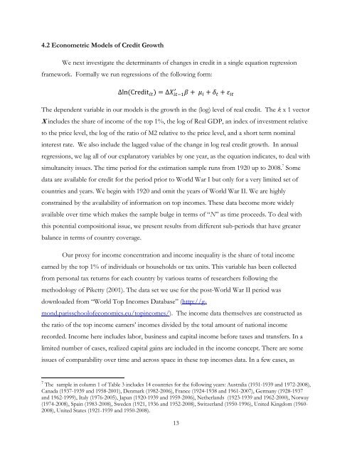
4.2 Econometric Models of Credit Growth We next investigate the determinants of changes in credit in a single equation regression framework. Formally we run regressions of the following form: � Δln�Credit�� Δ�� The dependent variable in our models is the growth in the (log) level of real credit. The k x 1 vector X includes the share of income of the top 1%, the log of Real GDP, an index of investment relative to the price level, the log of the ratio of M2 relative to the price level, and a short term nominal interest rate. We also include the lagged value of the change in log real credit growth. In annual regressions, we lag all of our explanatory variables by one year, as the equation indicates, to deal with simultaneity issues. The time period for the estimation sample runs from 1920 up to 2008. 7 Some data are available for credit for the period prior to World War I but only for a very limited set of countries and years. We begin with 1920 and omit the years of World War II. We are highly constrained by the availability of information on top incomes. These data become more widely available over time which makes the sample bulge in terms of “N” as time proceeds. To deal with this potential compositional issue, we present results from different sub-periods that have greater balance in terms of country coverage. Our proxy for income concentration and income inequality is the share of total income earned by the top 1% of individuals or households or tax units. This variable has been collected from personal tax returns for each country by various teams of researchers following the methodology of Piketty (2001). The data set we use for the post-World War II period was downloaded from “World Top Incomes Database” (http://gmond.parisschoolofeconomics.eu/topincomes/). The income data themselves are constructed as the ratio of the top income earners’ incomes divided by the total amount of national income recorded. Income here includes labor, business and capital income before taxes and transfers. In a limited number of cases, realized capital gains are included in the income concept. There are some issues of comparability over time and across space in these top incomes data. In a few cases, as 7 The sample in column 1 of Table 3 includes 14 countries for the following years: Australia (1931-1939 and 1972-2008), Canada (1937-1939 and 1958-2001), Denmark (1982-2006), France (1924-1938 and 1961-2007), Germany (1928-1937 and 1962-1999), Italy (1976-2005), Japan (1920-1939 and 1959-2006), Netherlands (1923-1939 and 1962-2000), Norway (1974-2008), Spain (1983-2008), Sweden (1921, 1936 and 1952-2008), Switzerland (1950-1996), United Kingdom (1960- 2008), United States (1921-1939 and 1950-2008). 13
mentioned, capital gains are included in the income concept. The definition of the tax unit also varies by country and over time. Some issues in comparability over time due to changes in tax laws have also been highlighted by Piketty and Saez who provided the web-based interface for the World Top Incomes Database. Despite these caveats, we follow Roine, Vlachos and Waldenström (2009) and pool these data as a reasonable first pass at the key relationships. 8 4.3 Credit Growth Determinants: Evidence from Five Year Periods Our first results rely on information from five-year periods as in Roine et. al. Annual volatility is significant in the data especially in the top income shares. Also this is an attempt to look at medium term trend relationships which is the horizon on which the RKR frameworks seem to be focused. An observation in this sample is thus the cumulative change over the previous five years for each variable. We restrict the sample to the endpoint of each quinquenium, and period dummies are included for each five year period to control for shocks. In these models, variables in the vector X are for the same five-year period. Table 2 presents four OLS regressions where the dependent variable is the cumulative growth over the previous five-years in the log of real credit. Column 1 includes only the cumulative percentage point change in the top income share as well as country fixed effects, time dummies, and growth in credit from the previous five-year period. While top income growth has a positive marginal effect, it is only significant at the 80 percent level of confidence. Column 2 adds the cumulative change in the log of real GDP over the previous five years to the model in column 1. Income growth is strongly related to credit growth. Again, we fail to reject the null hypothesis that top incomes have no association with the growth in credit. In column 3, we interact these two key variables. The reason is that the RKR hypothesis suggests that when total incomes and inequality are rising a credit boom arises in the bid to smooth consumption by the lower deciles. We find no evidence of such an impact with the interaction effect. Finally, column 4 controls for other macroeconomic fundamentals including the short-term nominal interest rate, the ratio of investment 8 We note that income inequality measures based on the Gini Coefficient or comparisons between the 90 th and the 10 th or the 50 th percentiles are different from the top incomes variable which captures only one part of the distribution. For checking the robustness of our results, we also investigated, but do not report results using the top 5% and the top 10% of earners. 14
Page 1 and 2: NBER WORKING PAPER SERIES DOES INEQ
Page 3 and 4: 1. Introduction The recent financia
Page 5 and 6: in the US and the fact that the med
Page 7 and 8: uncertainty about Federal Reserve a
Page 9 and 10: RKR frameworks. In fact, Borio and
Page 11 and 12: investigate it and confirm it in ou
Page 13: The goal here is to provide a simpl
Page 17 and 18: also robust to using ex post real i
Page 19 and 20: illion in credit and $85.1 billion
Page 21 and 22: 6. Conclusions Our paper looks for
Page 23 and 24: Goldin, C. Katz, L. 2008. The Race
Page 25 and 26: Table 1 Relationship Between Bankin
Page 27 and 28: Table 3 Explaining Changes in the l
Page 29 and 30: Figure 2 Changes in Bank Loans and

Michael D. Bordo Christopher M. Meissner Working Paper 178

Create successful ePaper yourself

Delete template?

Save as template?