DP2PN2Solver: A flexible dynamic programming solver software tool

Control and Cybernetics
vol. 35 (2006) No. 3
DP2PN2Solver: A flexible dynamic programming solver
software tool
by
Holger Mauch
Eckerd College, Natural Sciences Collegium
4200, 54th Ave. S., St. Petersburg, FL 33711, USA
e-mail: mauchh@eckerd.edu
Abstract: Dynamic programming (DP) is a very general optimization
technique, which can be applied to numerous decision
problems that typically require a sequence of decisions to be made.
The solver software DP2PN2Solver presented in this paper is a
general, flexible, and expandable software tool that solves DP problems.
It consists of modules on two levels. A level one module
takes the specification of a discrete DP problem instance as input
and produces an intermediate Petri net (PN) representation called
Bellman net (Lew, 2002; Lew, Mauch, 2003, 2004) as output — a
middle layer, which concisely captures all the essential elements of a
DP problem in a standardized and mathematically precise fashion.
The optimal solution for the problem instance is computed by an
“executable” code (e.g. Java, Spreadsheet, etc.) derived by a level
two module from the Bellman net representation.
DP2PN2Solver’s unique potential lies in its Bellman net representation.
In theory, a PN’s intrinsic concurrency allows to distribute
the computational load encountered when solving a single DP
problem instance to several computational units.
Keywords: Bellman net, dynamic programming, matrix chain
multiplication problem, optimization software, Petri net model, traveling
salesman problem.
1. Introduction
Operations Research (OR) deals with the efficient or optimal allocation of resources
and is thus of considerable importance in practice. For the optimization
of multistage decision processes dynamic programming (DP) is a powerful technique
to determine an optimal policy.
So far, software tools that would allow the user to conveniently state arbitrary
DP problems using the terminology and techniques that have been established
in the past in the DP field have not been developed. The solver software
DP2PN2Solver presented in this paper tries to fill this gap.

688 H. MAUCH
One of the difficulties in designing a DP solver system is to come up with
a specification language that is on the one hand general enough to capture the
majority of DP problems arising in reality, and that is on the other hand structured
enough to be parsed efficiently. For linear programming (LP) problems,
it is very easy to achieve both of these goals. For DP problems, however, it is
much harder to satisfy these conflicting goals. An intermediate problem representation
in the form of a Petri net (PN) model turns out to be a useful device
for this purpose. The model used is only applicable to “discrete” optimization
problems for which a DP functional equation with a finite number of states
and decisions can be obtained. Therefore, continuous DP problems cannot be
solved with DP2PN2Solver. The term “optimal solution” is used in this paper
not only for the optimal objective function value but also for the sequence of
optimal decisions leading to it.
The computational requirements of DP2PN2Solver are asymptotically the
same as the requirements for other DP codes implementing the DP functional
equation directly, since the intermediate PN model may be regarded as just
another representation of a DP functional equation. So for example, since a DP
solution of the traveling-salesman problem is inefficient (exponential-time), so
is a PN modeled solution.
The value of the DP2PN2Solver system becomes apparent when we survey
currently existing software supporting the solution of DP problems in Section 2.
There seems to be no system that can apply DP to a wide variety of problems.
Current software systems can only solve a narrow class of DP problems with a
rather simple DP functional equation.
DP2PN2Solver is illustrated by two typical DP problems. The interesting
feature of the first example problem, matrix chain multiplication (MCM), is that
there is not only one, but two successor states in its DP functional equation that
have to be evaluated. The second problem is the traveling salesman problem
(TSP), whose DP functional equation requires the use of set theoretic operators.
It will be demonstrated that DP2PN2Solver has no problems in dealing
with these problems which are slightly more complicated than finding, say, the
shortest path in a multistage graph (the standard textbook example for DP).
The organization of the paper is to start with a brief survey of existing
DP solver systems (Section 2), then to give the general architecture of our
DP2PN2Solver software (Section 3), followed by a more detailed description of
DP2PN2Solver’s modules (Sections 4 – 6) and to end with a short conclusion
section.
2. Other DP software systems
We briefly survey existing software systems that support the user in solving
instances of DP problems.
Attempts to develop general-purpose DP computer codes have been made in
the early 70’s by Hastings (1974) and others. While Hasting’s “DYNACODE”

Dynamic Programming with Petri net solver 689
is frequently referenced (e.g. in Hastings, 1973), detailed information about
this system is unavailable as of today. Sniedovich characterizes these codes as
problem specific and concludes that “no general-purpose dynamic programming
computer codes seem to be available commercially” (Sniedovich, 1992, p. 193).
Other, non-general DP codes have been developed in Hubert, Arabie, Meulman
(2001), Lin and Bricker (1990), Sniedovich (1993, 1994). DP software
accompanying textbooks such as Hillier and Lieberman (1990) does not generalize
well either. The shortcoming of these attempts is that they are usually
restricted to solve instances of one special problem.
Mailund’s DPROG system atwww.daimi.au.dk/~mailund assumes that the
user has a substantial amount of expertise in software engineering practice. As
of today it seems that major parts of the system are still under construction.
The optimization package system LINGO / LINDO solves optimization
problems across a wide problem domain with a variety of solution methods.
While its strength lies in the areas of linear programming, and to some extent
in integer programming and nonlinear programming, it is only of very limited
use to tackle DP problems. In particular, it is not obvious at all how to retrieve
the series of optimal decisions that lead to the optimal solution.
A disadvantage of this and many other optimization software systems is that
they incorporate search mechanisms. This can in the best case be very efficient,
but in the worst case not lead to the optimal solution at all.
The most common approach taken today for solving real-world DP problems
is to start a specialized software development project for each and every problem.
Even taking into account that a module-oriented development philosophy allows
considerable reuse of components, this is still a rather expensive approach. A
general solver solution like the DP2PN2Solver introduced here should be able
to save software development costs for many DP problems arising in practice.
3. DP2PN2Solver architecture
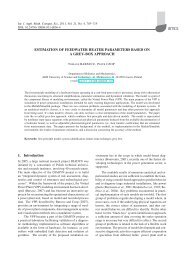
Fig. 1 gives an overview of the architecture of the DP2PN2Solver software tool
(in the form of a Petri net). The static components such as input files, intermediate
representations and output files are depicted as places. The dynamic
components such as compiler and code generator are shown as transitions. Solid
arcs connect fully working components while dotted arcs connect components
that are under construction and that should be available in future versions of
DP2PN2Solver.
DP2PN2Solver consists of modules on two levels. Level one modules
(gDP2PN, bDP2PN, etc.) take the specification of a discrete DP problem instance
as input and produce an intermediate Petri net (PN) representation
called Bellman net (Lew, 2002; Lew and Mauch, 2003, 2004) as output – a
middle layer, which concisely captures all the essential elements of a DP problem
in a standardized and mathematically precise fashion. Level two modules
(PN2Java, PN2XML, PN2Spreadsheet, etc.) take the intermediate Bellman net

690 H. MAUCH
DP specification
source file types
gDPS source
(.dp suffix)
bDPS source
AMPL source
gDP2PN
compiler
bDP2PN
compiler
... ...
internal
Bellman net
representation
PN2Java module
PN2XML module
...
PN2Spreadsheet
"Executable codes"
Java solver
code
PNML standard
file
Spreadsheet
file
Figure 1. Architecture of the DP2PN2Solver Tool
JRE
PN simulator
Spreadsheet
application
Solution of
DP Instance
Solution of
DP Instance
Solution of
DP Instance
representation as input and produce an “executable” solver code as output; that
is any kind of code from which the solution can be obtained in the next step.
E.g. a Java system could compile and interprete a Java source, a spreadsheet
application could open a spreadsheet file and calculate all cells, or a PN system
could simulate a PN provided in a standard XML-based PN file interchange
format.
To summarize, the following are the steps that need to be performed to
solve a DP problem instance; only step 1 is performed by the human DP modeler
whereas all other steps are automatically performed by the DP2PN2Solver
system.
1. Model the real-world problem and create the DP specification file, for
example in the gDPS language (see Section 4).
2. The appropriate DP2PN module produces the intermediate Bellman net
representation (see Section 5).
3. One of the PN2Solver modules produces runnable Java code, or a spreadsheet
or another form of executable solver code, which is capable of solving
the problem instance.
4. Run the resulting executable solver code and output the solution of the
problem instance (see Section 6).
4. The DP specification language
DP problems can can take on various forms and shapes. This is why it is hard to
specify a strict and fixed specification format like for linear programming (LP).
But there are common themes across all DP problems and those are captured
in the general DP specification (gDPS) language.
A special purpose language should allow for both a convenient description

Dynamic Programming with Petri net solver 691
of a DP problem instance and efficient parsing of the specification. The gDPS
language has been designed as a general source language that can describe a
variety of DP problems. It offers the flexibility needed for the various types of
DP problems that arise in reality. Sources in gDPS for the matrix chain multiplication
and for the traveling salesman problem are given in Subsections 4.1
and 4.2, respectively. Other DP problems that have been successfully modelled
with gDPS and solved by DP2PN2Solver include the shortest path problem
(cyclic graphs allowed), reliability design problems (with multiplication operator
in DP functional equation), the longest common subsequence problem, the
optimal edit distance problem, the optimal binary search tree problem, and
many more.
A gDPS consists of several structured sections, which reflect the standard
parts of every DP problem. To increase writability, additional information such
as helper functions that ease the DP model formulation can be included into a
gDPS source. Of particular importance are the following sections.
• The optionalGENERAL_VARIABLES section allows the definition of variables
(e.g. of type int, double, or String) in a C++/Java style syntax.
• The optional SET_VARIABLES section allows the definition of variables of
type Set (which can take on a set of integers as value) in a convenient
enumerative fashion the way it is written in mathematics. Ellipsis is supported
with a subrange syntax.
• The optionalGENERAL_FUNCTIONSsection allows the definition of arbitrary
functions in a C++/Java style syntax.
• The mandatory STATE_TYPE section. A state in a DP problem can be
viewed as an ordered tuple of variables. The variables can be of heterogeneous
types. The “stage” of a DP problem would, as an integer coordinate
of its state, be one part of the ordered tuple.
• The mandatory DECISION_VARIABLE and DECISION_SPACE sections declare
the type of a decision and the set of decisions from which to choose
(the space of alternatives), which is given as a function of the state.
• The mandatory DP functional equation (DPFE). The recursive equation
is described in the DPFE section and its base cases must either be expressed
in conditional fashion in the DPFE_BASE_CONDITIONS or in a enumerative
way in the DPFE_BASE section.
• The computational goal of the DP instance is given in the mandatoryGOAL
section.
• The reward function (cost function) is given as a function of the state and
the decision in the mandatory REWARD_FUNCTION section.
• The transformation functions (one or more) are given as functions of the
state and the decision in the mandatory TRANSFORMATION_FUNCTION section.
Set theoretic features in the gDPS language simplify the specification and
improve its readability. A variable of the type Set can be declared in the

692 H. MAUCH
SET_VARIABLES section. Such variables and set literals (described using complete
enumeration, or a subrange syntax) can be operands of set theoretic operations
like SETUNION, SETINTERSECTION or SETMINUS.
Throughout a gDPS source it is legal to document it using C++/Java style
block comments (between /* and */) and line comments (starting with //).
Since the GENERAL_VARIABLES section allows the definition of arbitrary variables
and the GENERAL_FUNCTIONS section allows the definition of arbitrary
(computable) functions in a C++/Java style syntax, the gDPS language is powerful
and flexible. Despite this power and flexibility, the other sections require
a very structured format, which makes a gDPS very readable and produces a
specification that resembles the mathematical formulation closely. The hybrid
approach of flexible C++/Java style elements and strictly structured sections
makes it easy to learn the gDPS language.
Input data that is specific to a DP instance is hardwired into the gDPS
source in order to have a single gDPS source file that contains the complete
specification of the DP instance. If it seems more desirable to keep separate
files for the instance specific data and the problem specific data, this would
require a conceptually straightforward modification which we will not elaborate
on any further here.
DP2PN2Solver’s architecture is expandable and open to alternative source
DP specification languages (see figure 1). For example, if the user desires to
solve only very basic DP problems that involve only integer types as states or
decisions, so that declarations are not necessary, then a much simpler language,
the basic DP specification (bDPS) language, is sufficient. By adding a compiler
to DP2PN2Solver that translates the bDPS into the Bellman net representation
it becomes possible to use the other parts of the DP2PN2Solver system without
any further changes. Even compilers for established mathematical programming
languages like AMPL, GAMS, OPL, or other languages mentioned in section 2
can be envisioned. Those could easily be integrated into DP2PN2Solver (even
though the development of the compiler itself might require a substantial initial
implementation effort), so that users can write the DP specification in their
favorite language.
4.1. The matrix chain multiplication (MCM) problem example
Given a product A1A2 · · · An of matrices of various (but still compatible) dimensions,
the goal is to find a parenthesization, which minimizes the number of
componentwise multiplications. The dimensions of Ai are denoted by di−1 and
di. The DP functional equation can be expressed as
�
min
f(i, j) = k∈{i,...,j−1} {f(i, k) + f(k + 1, j) + di−1dkdj} if i < j
0 if i = j.
The total number of componentwise multiplications is computed as f(1, n).
(1)

Dynamic Programming with Petri net solver 693
For instance, let n = 4 and (d0, d1, d2, d3, d4) = (3, 4, 5, 2, 2). Apply the DP
functional equation (1) in a bottom up fashion to compute f(1, 4) = 76. By
keeping track of which arguments minimize the min-expressions in each case,
one arrives at the optimal parenthesization ((A1(A2A3))A4).
This DP problem instance can be coded in gDPS as follows:
BEGIN
NAME MCM; //Matrix Chain Multiplication
END
GENERAL_VARIABLES_BEGIN
//dimensions in Matrix Chain Multiplication problem
private static int[] dimension = {3, 4, 5, 2, 2};
private static int n = dimension.length-1; //n=4 matrices
GENERAL_VARIABLES_END
STATE_TYPE: (int firstIndex, int secondIndex);
DECISION_VARIABLE: int k;
DECISION_SPACE: decisionSet(firstIndex,secondIndex)
={firstIndex,..,secondIndex - 1};
GOAL: f(1,n);
DPFE_BASE_CONDITIONS:
f(firstIndex,secondIndex)=0.0 WHEN (firstIndex==secondIndex);
DPFE: f(firstIndex,secondIndex)
=MIN_{k IN decisionSet}
{ f(t1(firstIndex,secondIndex,k))
+f(t2(firstIndex,secondIndex,k))
+r(firstIndex,secondIndex,k)
};
REWARD_FUNCTION: r(firstIndex,secondIndex,k)
=dimension[firstIndex - 1]
*dimension[k]*dimension[secondIndex];
TRANSFORMATION_FUNCTION: t1(firstIndex,secondIndex,k)
=(firstIndex,k);
t2(firstIndex,secondIndex,k)
=(k+1,secondIndex);

694 H. MAUCH
4.2. The traveling salesman problem (TSP) example
Given a complete weighted directed graph G = (V, E) with distance matrix
C = (ci,j) the optimization version of the traveling saleman problem asks to
find a minimal Hamiltonian cycle (visiting each of the n = |V | vertices exactly
once). Without loss of generality assume V = {0, . . ., n−1}. The DP functional
equation can be expressed as
f(v, S) =
� min
d/∈S {f(d, S ∪ {d}) + cv,d} if |S| < n
cv,s
if |S| = n
where the length of the minimal cycle is computed as f(s, {s}), with s ∈ V .
(The choice of the starting vertex s is irrelevant, since we are looking for a
cycle, so arbitrarily pick s = 0.) In the above DP functional equation (2), a
state is a pair (v, S) where v can be interpreted as the current vertex and S as
the set of vertices already visited.
For instance, let
⎛
⎜
C = ⎜
⎝
0 1 8 9 60
2 0 12 3 50
7 11 0 6 14
10 4 5 0 15
61 51 13 16 0
⎞
⎟
⎠ .
Apply the DP functional equation (2) to compute f(0, {0}) = 39. By keeping
track of which arguments minimize the min-expressions in each case, we find
that the minimal cycle is (0, 1, 3, 4, 2).
Note the convenient use of variables and literals of the type Set in the
following gDPS example for this problem instance.
BEGIN
NAME TSP; //TravelingSalesmanProblem;
GENERAL_VARIABLES_BEGIN
//adjacency matrix for TSP.
private static int[][] distance =
{
{ 0, 1, 8, 9, 60},
{ 2, 0, 12, 3, 50},
{ 7, 11, 0, 6, 14},
{10, 4, 5, 0, 15},
{61, 51, 13, 16, 0}
};
private static int n = distance.length;
//number of nodes n=5. Nodes are named starting
//at index 0 through n-1.
(2)

Dynamic Programming with Petri net solver 695
END
GENERAL_VARIABLES_END
SET_VARIABLES_BEGIN
Set setOfAllNodes={0,..,n - 1};
Set goalSet={0};
SET_VARIABLES_END
STATE_TYPE: (int currentNode, Set nodesVisited);
DECISION_VARIABLE: int d;
DECISION_SPACE: nodesNotVisited(currentNode,nodesVisited)
=setOfAllNodes SETMINUS nodesVisited;
GOAL:
f(0,goalSet); //that is: (0,{0});
DPFE_BASE_CONDITIONS:
f(currentNode, nodesVisited)
=distance[currentNode][0]
WHEN (nodesVisited SETEQUALS setOfAllNodes);
DPFE: f(currentNode,nodesVisited)
=MIN_{d IN nodesNotVisited}
{ cost(currentNode,nodesVisited,d)
+f(t(currentNode,nodesVisited,d))};
REWARD_FUNCTION: cost(currentNode,nodesVisited,d)
=distance[currentNode][d];
TRANSFORMATION_FUNCTION: t(currentNode,nodesVisited,d)
=(d, nodesVisited SETUNION {d});
5. The intermediate Bellman net representation
Familiarity with basic Petri net terminology is assumed in this paper. Detailed
introductions to PNs are Reisig (1985) and Murata (1989). For colored PNs,
see Jensen (1992).
The details for the Bellman nets used in DP2PN2Solver are described in
Lew (2002), Lew and Mauch (2003, 2004). The most important features are
summarized in this section.
A Bellman net is a special high-level colored Petri net with the following
properties.

696 H. MAUCH
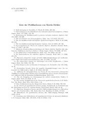
1. The color type is numerical in nature, tokens are real numbers. In addition,
single black tokens, depicted [] in Fig. 2, are used to initialize
enabling places, which are technicalities that prevent transitions from firing
more than once.
2. A place contains at most one token at any given time.
3. The postset of a transition contains exactly one designated output place,
which contains the result of the computational operation performed by
the transition. (In the example Bellman nets shown in Figs. 2 and 3
designated output places are labeled p1 throughp16, base state places are
labeled p17 through p20, and enabling places are not labeled.)
4. There are two different types of transitions, namely M-transitions and
E-transitions. An M-transition performs a minimization or maximization
operation using the tokens of the places in its preset as operands and puts
the result into its designated output place. An E-transition evaluates a
basic arithmetic expression (involving operators like addition or multiplication)
using fixed constants and tokens of the places in its preset as
operands and puts the result into its designated output place. (In the
example Bellman nets shown in Figs. 2 and 3 M-transitions are labeled m1
through m6, E-transitions are labeled s1 through s10.)
5. There are self-loops between an E-transition and all places in its preset.
Their purpose is to conserve operands serving as input for more than one
E-transition.
A numerical token as the marking of a place in a Bellman net can be interpreted
as an intermediate value that is computed in the course of calculating
the solution of a corresponding DP problem instance.
For example, the Bellman net of the MCM problem instance, in its initial
marking, is depicted in Fig. 2.
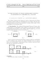
To obtain the final marking of the Bellman net, fire transitions until the net
is dead. The net in its final marking is depicted in Fig. 3. Note that the goal
state place p1 contains f(1, 4) = 76 tokens now, the correct value indeed. Also,
the marking of an intermediate state place represents the optimal value for the
associated subproblem. For example, the value of the intermediate state place
p6 is f(2, 4) = 56 which is the number of componentwise multiplications for the
optimally parenthesized matrix product A2 · · · A4
Note that the order in which transitions fire is not relevant for the value of
the final result f(1, 4).
Note also how the intermediate Bellman net representation gives an illustrative
graphical representation of the problem instance. Also, since there is
an abundance of PN theory that allows to examine certain properties of PNs
like circularity, liveness, etc. there is the chance for extensive automated consistency
checks on the PN level which could unveil certain mistakes made by the
DP modeler when giving the DP specification.

Figure 2. Bellman net in its initial marking for the MCM problem instance
p1
f(1,4)
y
m1
p2
y=Math.
min(x1,Math.
min(x2,x3))
x1
x2
x3
p4
p3
[]
s1
y=x1+x2+24
y
[]
y y=x1+x2+30
y
x2
s2
x1
y=x1+x2+12
[]
s3
f(1,3)
f(2,4)
p5
p6
x1
x1
y
x2
y
x2
m2
y=Math.
min(x1,x2)
m3
y=Math.
min(x1,x2)
x1
x2
x1
p7
p8
x2
p9
p10
y
y
y
[]
s4
y=x1+x2+24
y
s7
x2
[]
s5
x1
y=x1+x2+30
x1
[] s6
x2
y=x1+x2+40
x2
[]
x1
y=x1+x2+16
x1
p11
x
f(1,2)
p12
x
f(2,3)
p13
x
f(3,4)
x2
m4
m5
m6
x
x
x
p14
p15
p16
y
y
y
[]
s8
y=x1+x2+60
[]
s9
y=x1+x2+40
[] s10
y=x1+x2+20
x1
x2
x1
x2
x1
x2
p17
0 f(1,1)
p18
0 f(2,2)
p19
0 f(3,3)
p20
0
f(4,4)
Dynamic Programming with Petri net solver 697

Figure 3. Bellman net in its final marking for the MCM problem instance
p1
76
f(1,4)
y
m1
p2
y=Math.
min(x1,Math.
min(x2,x3))
x1
x2
x3
p4
p3
s1
y=x1+x2+24
y
y y=x1+x2+30
y
x2
s2
x1
y=x1+x2+12
s3
p5
x1
f(1,3) 64 y
x1
x2
f(2,4) 56 y
p6
x2
m2
y=Math.
min(x1,x2)
m3
y=Math.
min(x1,x2)
x1
x2
x1
p7
p8
x2
p9
p10
y
y
y
y
s4
y=x1+x2+24
s7
x2
x1
s5
y=x1+x2+30
x1
s6
x2
y=x1+x2+40
x2
x1
y=x1+x2+16
x1
p11
60 x
f(1,2)
p12
40 x
f(2,3)
p13
20 x
f(3,4)
x2
m4
m5
m6
x
x
x
p14
p15
p16
y
y
y
s8
y=x1+x2+60
s9
y=x1+x2+40
s10
y=x1+x2+20
x1
x2
x1
x2
x1
x2
p17
0 f(1,1)
p18
0 f(2,2)
p19
0 f(3,3)
p20
0
f(4,4)
698 H. MAUCH

Dynamic Programming with Petri net solver 699
In contrast to the Bellman net model described here, Mauch (2004) describes
a non-colored PN approach that can also be used as an intermediate representation
of DP problem instances. While the expressional power of both approaches
seems to be equivalent (no proof yet) it is easier to transform Bellman nets
to executable computer code. However, the low level PN model introduced in
Mauch (2004) is easier to examine with respect to consistency, and other net
theoretic issues. If the equivalence of the two models can be shown, and a practical
transformation algorithm between the two models can be designed, then
one could take advantage of the benefits of both models.
Current standardization efforts (see Billington et al., 2003) introduce the
Petri Net Markup Language (PNML) as an XML-based interchange format for
PNs. Although the PNML standard still undergoes changes, DP2PN2Solver
contains a module PN2XML that is capable of producing a standard file format
from a Bellman net. By importing the standard file into a PN simulator like
Renew (Kummer, Wienberg, Duvigneau, 2002) this opens up the possibility to
simulate the Bellman net with external PN systems. Now the user can watch
how a DP problem instance is solved in an illustrative graphical fashion by observing
the simulation progress. The shortcomings of solving DP problems in
this way are performance penalties due to the overhead of the PN simulation
system, and the fact that only the optimal value of the solution is observable,
but not the decisions leading to the optimum. Therefore the following section
discusses the PN2Java module of DP2PN2Solver which overcomes these problems.
6. The solution code
The PN2Java module of DP2PN2Solver generates Java sources that efficiently
produce the optimal solution to the underlying DP problem instance, along with
the series of optimal decisions leading to it. (Note the use of the term “efficient”
in this context. If the underlying DP problem is inherently inefficient — as in
the TSP example — then PN2Java will produce an inefficient output. The point
made here is that the transformation process itself is efficient.) A Java-based
solver code takes advantage of the ubiquitous and free availability of the Java
compile and run-time system. PN2Java also ensures that the produced code is
well commented and human-readable, so it is possible to verify its correctness,
or use the code as a building block for a larger software development project.
Executing the bare Java code without any further modifications leads to the
following output for the two examples introduced earlier.
The solution for the MCM problem example:
The optimal value is: 76.0
The solution tree is:
State (1,4) has optimal value: 76.0
Decision k=3

700 H. MAUCH
State (1,3) has optimal value: 64.0
Decision k=1
Base state (1,1) has initial value: 0.0
State (2,3) has optimal value: 40.0
Decision k=2
Base state (2,2) has initial value: 0.0
Base state (3,3) has initial value: 0.0
Base state (4,4) has initial value: 0.0
The solution for the TSP problem example:
The optimal value is: 39.0
The solution tree is:
State (0,{0}) has optimal value: 39.0
Decision d=1
State (1,{0,1}) has optimal value: 38.0
Decision d=3
State (3,{0,1,3}) has optimal value: 35.0
Decision d=4
State (4,{0,1,3,4}) has optimal value: 20.0
Decision d=2
Base state (2,{0,1,2,3,4}) has initial value: 7.0
The TSP is NP-complete, and the time complexity of DP2PN2Solver for
TSP is exponential in the number n of vertices in the graph. This is inherent
in the formulation of TSP as a DP problem.
As an alternative to the presented PN2Java module one could envision a
module that transforms the Bellman net directly into machine code (for applications
that require the utmost performance at the expense of machine independence).
Another idea is to translate the Bellman net into a spreadsheet
file. Spreadsheet formats are quite popular in the OR community and in management
science, and a graphically appealing output of the optimal decisions
within a spreadsheet should be a valuable tool for decision makers. Such a
module (PN2Spreadsheet) is currently under construction.
7. Conclusion
With DP2PN2Solver it becomes possible to automatically solve many optimization
problems of practical relevance with DP. This constitutes a considerable
improvement of today’s use of DP, where usually for each problem at hand specialized
software development takes place. The DP2PN2Solver user no longer
needs deep skills in software development to solve a problem. After gaining insight
into the nature of the real-world problem to be solved, the user can focus
on the important modeling process and come up with a precise DP specification
(in particular the DP functional equation) of the problem. It is no longer

Dynamic Programming with Petri net solver 701
necessary to worry about the DP solution process itself, since DP2PN2Solver
automates all other steps.
DP2PN2Solver guarantees that the optimal solution to a DP instance will
be found, provided of course that the DP functional equation is correct and its
solution does exist.
The gDPS language is easy to learn, so DP2PN2Solver should also be a
great educational tool for teaching DP in a practical hands on approach, where
students can work on case studies, model the underlying DP problem, and get
an actual solution to the problem without the need to worry too much about
the solution process itself.
The structured design of the gDPS language allows for the addition of a
straightforward graphical user input mask as a frontend to make the modeling
of the DP specification even more convenient in future versions.
References
Billington, J., Christensen, S., Hee, K.V., Kindler, E., Kummer, O.,
Petrucci, L., Petrucci, L., Post, R., Stehno, C., and Weber,
M. (2003) The Petri net markup language: Concepts, technology, and
tools. In: W. van der Aalst and E. Best, eds., ICATPN 2003, LNCS,
2679, Springer-Verlag, 483–505.
Hastings, N. (1973) Dynamic programming with management applications.
Butterworths, London, England, 1973.
Hastings, N. (1974) DYNACODE dynamic programming systems handbook.
Management Center, University of Bradford, Bradford, England.
Hillier, F.S. and Lieberman, G.J. (1990) Introduction to operations research,
5th edition. McGraw-Hill Publishing Company. New York.
Hubert, L.J., Arabie, P. and Meulman, J. (2001) Combinatorial data
analysis: Optimization by dynamic programming. Society for Industrial
and Applied Mathematics (SIAM). Philadelphia, PA.
Jensen, K. (1992) Coloured Petri Nets, Vol. 1. Springer-Verlag.
Kummer, O., Wienberg, F., and Duvigneau, M. (2002) Renew User
Guide Release 1.6. Department of Informatics. University of Hamburg,
Hamburg, Germany.
Lew, A. (2002) A Petri net model for discrete dynamic programming. In:
Proceedings of the 9th Bellman Continuum: International Workshop on
Uncertain Systems and Soft Computing. Beijing, China, July 24–27, 16–
21.
Lew, A. and Mauch, H. (2003) Solving integer dynamic programming using
Petri nets. In: Proceedings of the Multiconference on Computational
Engineering in Systems Applications (CESA). July 9–11, Lille, France.
Lew, A. and Mauch, H. (2004) Bellman nets: A Petri net model and tool for
dynamic programming. In: Proceedings of Modelling, Computation and
Optimization in Information Systems and Management Sciences (MCO).

702 H. MAUCH
July 1–3, Metz, France.
Lin, E.Y. and Bricker, D.L. (1990) Implementing the recursive APL code
for dynamic programming. APL Quote Quad 20 (4), 239–250.
Mauch, H. (2004) A Petri net representation for dynamic programming problems
in management applications. In: Proceedings of the 37th Hawaii International
Conference on System Sciences (HICSS2004). January 5–8,
Waikoloa, Hawaii. IEEE Computer Society.
Murata, T. (1989) Petri nets: Properties, analysis and applications. Proceedings
of the IEEE 77 (4), 541–580.
Reisig, W. (1985) Petri Nets: an Introduction. Springer-Verlag, Berlin.
Sniedovich, M. (1992) Dynamic programming. Marcel Dekker, Inc., New
York.
Sniedovich, M. (1993) A dynamic programming algorithm for the travelling
salesman problem. ACM SIGAPL APL Quote Quad 23 (4), 1–3.
Sniedovich, M. (1994) Dynamic programming algorithms for the knapsack
problem. ACM SIGAPL APL Quote Quad 24 (3), 18–21.