Agilent 1100/1200 HPLC ChemStation Operation
Agilent 1100/1200 HPLC ChemStation Operation
Agilent 1100/1200 HPLC ChemStation Operation

You also want an ePaper? Increase the reach of your titles
YUMPU automatically turns print PDFs into web optimized ePapers that Google loves.
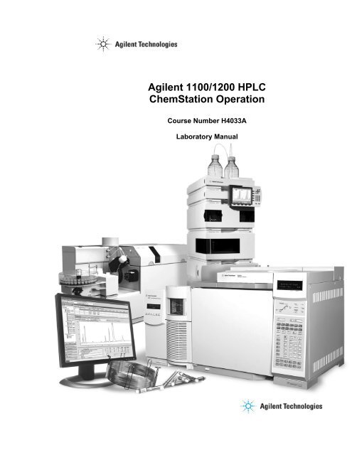
<strong>Agilent</strong> <strong>1100</strong>/<strong>1200</strong> <strong>HPLC</strong><br />
<strong>ChemStation</strong> <strong>Operation</strong><br />
Course Number H4033A<br />
Laboratory Manual
<strong>Agilent</strong> <strong>1100</strong>/<strong>1200</strong> <strong>HPLC</strong><br />
<strong>ChemStation</strong> <strong>Operation</strong><br />
Course Number H4033A<br />
Laboratory Manual<br />
<strong>ChemStation</strong> B.03<br />
Printed in April, 2007
Notice<br />
The information contained in this document is subject to change without notice.<br />
<strong>Agilent</strong> Technologies makes no warranty of any kind with regard to this material,<br />
including but not limited to the implied warranties of merchantability and fitness<br />
for a particular purpose.<br />
<strong>Agilent</strong> Technologies shall not be liable for errors contained herein or for<br />
incidental, or consequential damages in connection with the furnishing,<br />
performance, or use of this material.<br />
No part of this document may be photocopied or reproduced, or translated to<br />
another program language without the prior written consent of <strong>Agilent</strong><br />
Technologies, Inc.<br />
<strong>Agilent</strong> Technologies, Inc<br />
3750 Brookside Pkwy<br />
Suite 100<br />
Alpharetta, GA 30022<br />
ii<br />
© 2007 by <strong>Agilent</strong> Technologies, Inc.<br />
All rights reserved<br />
Printed in the United States of America
Table Of Contents<br />
LAB EXERCISE: INTRODUCTION TO THE <strong>HPLC</strong> CHEMSTATION..... 1<br />
IN THIS LABORATORY YOU WILL: ....................................................................... 2<br />
ACCESSING THE <strong>HPLC</strong> CHEMSTATION................................................................ 3<br />
CONFIGURATION EDITOR ..................................................................................... 5<br />
SCHEDULER ......................................................................................................... 6<br />
MAINTAINING THE WINDOWS 2000 WORKSTATION ............................................ 8<br />
Cleaning up Temporary Files ......................................................................... 8<br />
Repairing the Disk .......................................................................................... 8<br />
Disk Defragmentation..................................................................................... 9<br />
Creating an Emergency Repair Disk .............................................................. 9<br />
MAINTAINING THE WINDOWS XP WORKSTATION ............................................. 10<br />
Cleaning up Temporary Files ....................................................................... 10<br />
Repairing the Disk ........................................................................................ 10<br />
Disk Defragmentation................................................................................... 11<br />
Creating an Emergency Repair Disk ............................................................ 11<br />
WINDOWS FEATURES (WINDOWS 2000 OR XP) ................................................. 13<br />
Windows Explorer......................................................................................... 13<br />
Wallpaper and Screen Savers ....................................................................... 14<br />
Clipboard ...................................................................................................... 15<br />
Closing a Program that is Not <strong>Operation</strong>al ................................................. 15<br />
LAB EXERCISE: ACQUISITION METHODS............................................. 17<br />
IN THIS LABORATORY YOU WILL: ..................................................................... 18<br />
PREPARATION .................................................................................................... 19<br />
PREPARING THE <strong>HPLC</strong> ...................................................................................... 20<br />
PRIMING THE AGILENT <strong>1100</strong>/<strong>1200</strong> SOLVENT DELIVERY SYSTEM ...................... 21<br />
CREATING AN ACQUISITION METHOD................................................................ 23<br />
PRACTICE ENTERING GRADIENTS ...................................................................... 24<br />
SNAPSHOT.......................................................................................................... 27<br />
LAB EXERCISE: QUALITATIVE DATA ANALYSIS................................ 29<br />
IN THIS LABORATORY YOU WILL: ..................................................................... 30<br />
GRAPHICS - SIGNAL OPTIONS............................................................................. 31<br />
GRAPHICS - ANNOTATION.................................................................................. 33<br />
WINDOW FUNCTIONS......................................................................................... 35<br />
PEAK PURITY ..................................................................................................... 36<br />
AUTOMATED PEAK PURITY................................................................................ 38<br />
DISPLAYING SPECTRA........................................................................................ 39<br />
ISOABSORBANCE PLOT....................................................................................... 40<br />
3D PLOT ............................................................................................................ 42<br />
iii
LAB EXERCISE: SPECTRAL LIBRARIES .................................................. 43<br />
IN THIS LABORATORY YOU WILL: ..................................................................... 44<br />
BUILDING A LIBRARY ........................................................................................ 45<br />
LIBRARY SEARCHING......................................................................................... 47<br />
LAB EXERCISE: OVERVIEW AND DIAGNOSTICS ................................. 49<br />
IN THIS LABORATORY YOU WILL: ..................................................................... 50<br />
Overview of Equipment and Tools Used....................................................... 50<br />
Consumables................................................................................................. 50<br />
THE AGILENT <strong>1200</strong> FLOW PATH ........................................................................ 51<br />
ERROR MESSAGES AND THE LOGBOOK.............................................................. 52<br />
DIAGNOSIS VIEW ............................................................................................... 53<br />
ROUTINE MAINTENANCE ................................................................................... 59<br />
INSTRUMENT TESTS ........................................................................................... 60<br />
LAB EXERCISE: OVERVIEW AND DIAGNOSTICS FOR THE<br />
AGILENT-SL SERIES....................................................................................... 61<br />
IN THIS LABORATORY YOU WILL: ..................................................................... 62<br />
Overview of Equipment and Tools Used....................................................... 62<br />
Consumables................................................................................................. 62<br />
THE AGILENT <strong>1200</strong> - SL FLOW PATH................................................................. 63<br />
ERROR MESSAGES AND THE LOGBOOK.............................................................. 64<br />
AGILENT LC DIAGNOSTIC TOOL........................................................................ 65<br />
INSTRUMENT STATUS REPORT ........................................................................... 69<br />
ROUTINE MAINTENANCE ................................................................................... 70<br />
INSTRUMENT TESTS ........................................................................................... 71<br />
LAB EXERCISE: INTEGRATION................................................................. 73<br />
IN THIS LABORATORY YOU WILL: ..................................................................... 74<br />
INTEGRATION PREPARATION.............................................................................. 75<br />
AUTO INTEGRATION........................................................................................... 76<br />
INTEGRATE USING THE EVENTS TABLE ............................................................. 78<br />
ADDING TIMED EVENTS..................................................................................... 79<br />
USING MANUAL EVENTS ................................................................................... 81<br />
LAB EXERCISE: QUANTIFICATION.......................................................... 83<br />
IN THIS LABORATORY YOU WILL: ..................................................................... 84<br />
PREPARATIONS .................................................................................................. 85<br />
CREATING THE ACQUISITION METHOD .............................................................. 87<br />
DATA ACQUISITION-STANDARDS....................................................................... 89<br />
INTEGRATION..................................................................................................... 91<br />
SETTING UP SIGNAL DETAILS............................................................................. 93<br />
BUILDING A CALIBRATION TABLE ..................................................................... 94<br />
SETTING UP LOW AND HIGH AMOUNT LIMITS FOR CALIBRATION STANDARDS . 96<br />
SETTING UP QUALIFIERS (DIODE ARRAY ONLY) ................................................ 97<br />
TESTING THE CALIBRATION TABLE.................................................................... 98<br />
iv
LAB EXERCISE: RUNNING A SEQUENCE................................................ 99<br />
IN THIS LABORATORY YOU WILL: ................................................................... 100<br />
BUILDING A SEQUENCE.................................................................................... 101<br />
SEQUENCE SUMMARY REPORTS....................................................................... 104<br />
STARTING THE SEQUENCE................................................................................ 105<br />
PAUSING A SEQUENCE ..................................................................................... 106<br />
POST SEQUENCE............................................................................................... 107<br />
LAB EXERCISE: SEQUENCE REVIEW AND REPROCESSING.......... 109<br />
IN THIS LABORATORY YOU WILL: ................................................................... 110<br />
REPROCESS WITH SEQUENCE FOLDER METHOD............................................... 111<br />
REPROCESS WITH DA METHODS...................................................................... 117<br />
BATCH REVIEW................................................................................................ 121<br />
LAB EXERCISE: ADVANCED REPORTING ........................................... 123<br />
IN THIS LABORATORY YOU WILL: ................................................................... 124<br />
ADDING A REPORT HEADER............................................................................. 125<br />
PERFORMANCE REPORTS (SYSTEM SUITABILITY) ............................................ 127<br />
AUTOMATED PEAK PURITY.............................................................................. 129<br />
AUTOMATED SPECTRAL LIBRARY SEARCH...................................................... 130<br />
LAB EXERCISE: CUSTOMIZED REPORT DESIGN ............................... 133<br />
IN THIS LABORATORY YOU WILL: ................................................................... 134<br />
PREPARATIONS ................................................................................................ 135<br />
BUILDING A CUSTOMIZED REPORT .................................................................. 136<br />
ADDING A GENERAL SECTION.......................................................................... 137<br />
INSERTING TABLES .......................................................................................... 138<br />
ADDING A CALIBRATION CURVE ..................................................................... 139<br />
FINISHING UP................................................................................................... 140<br />
LAB EXERCISE: COMMANDS ................................................................... 141<br />
IN THIS LABORATORYYOU WILL: .................................................................... 142<br />
RETRIEVING INFORMATION ABOUT COMMANDS .............................................. 143<br />
TRACKING ERRORS AND USING SOME COMMON COMMANDS.......................... 144<br />
REGISTERS, OBJECTS, AND TABLES ................................................................. 145<br />
LAB EXERCISE: MACRO WRITING ........................................................ 153<br />
IN THIS LABORATORY YOU WILL: ................................................................... 154<br />
WRITING AND EXECUTING A MACRO............................................................... 155<br />
WRITE YOUR OWN MACRO ............................................................................. 157<br />
POSSIBLE ANSWER........................................................................................... 158<br />
APPENDIX: GETTING STARTED WITH NEW CHEMSTATION<br />
WORKFLOW G2170-90041........................................................................... 159<br />
v
Lab Exercise: Introduction to the <strong>HPLC</strong><br />
<strong>ChemStation</strong>
Lab Exercise: Introduction to the <strong>HPLC</strong> <strong>ChemStation</strong><br />
In this Laboratory You Will:<br />
In this Laboratory You Will:<br />
• Access the <strong>HPLC</strong> <strong>ChemStation</strong> software and understand the purpose of each<br />
View.<br />
• Use the <strong>ChemStation</strong> Configuration Editor.<br />
• Learn about the Scheduler.<br />
• Learn how to maintain the <strong>HPLC</strong> <strong>ChemStation</strong> computer.<br />
• Become familiar with some Windows features (optional).<br />
2
Accessing the <strong>HPLC</strong> <strong>ChemStation</strong><br />
Lab Exercise: Introduction to the <strong>HPLC</strong> <strong>ChemStation</strong><br />
Accessing the <strong>HPLC</strong> <strong>ChemStation</strong><br />
1) Find the Start button in the bottom left hand corner of your screen. Click on<br />
the Start button. Select the menu choice All Programs. You will find a list<br />
of the software programs installed on this computer arranged in alphabetical<br />
order. To launch the <strong>ChemStation</strong> for LC 3D Systems, find and select the<br />
<strong>Agilent</strong> <strong>ChemStation</strong> menu item.<br />
2) The following items are available: Add Licenses, Configuration Editor,<br />
Installation Qualification, Instrument 1 Online, Instrument 1 Offline,<br />
readme.txt, and the Scheduler.<br />
3) Click on Instrument 1 Offline. The software program will begin loading.<br />
Question:<br />
What is the difference between the <strong>ChemStation</strong>'s Online and Offline sessions?<br />
_________________________________________________________________<br />
_________________________________________________________________<br />
4) Open the View menu and select Full Menu, if this item is available.<br />
5) Access the View menu and examine the entries. Notice that there are several<br />
main views starting with Method and Run Control. List the views below<br />
and after exploring each view, list the primary function of each.<br />
View Function<br />
3
Lab Exercise: Introduction to the <strong>HPLC</strong> <strong>ChemStation</strong><br />
Accessing the <strong>HPLC</strong> <strong>ChemStation</strong><br />
6) You can also change views by utilizing the Navigation Buttons.<br />
Switch Views Here Minimize, Maximize<br />
4<br />
Close<br />
7) Click on the small triangle at the top of the <strong>ChemStation</strong> Explorer. Click<br />
again. Notice that you can sort your files.<br />
8) Click on the Configure buttons icon at the bottom of the Navigation Pane –<br />
you can use this to add or remove buttons.<br />
9) Find the Minimize, Maximize and Close buttons located in the upper right<br />
hand corner of the Title Bar. Minimize the <strong>ChemStation</strong> software. Notice<br />
that the <strong>ChemStation</strong> software now appears as a button to the right of the<br />
Windows Start button in the Task Bar. The <strong>ChemStation</strong> software is still<br />
running, but has been cleared from the Desktop.<br />
10) Click on the Instrument 1 (offline) software button in the Task Bar to restore<br />
the <strong>ChemStation</strong> window.<br />
11) To close the <strong>ChemStation</strong> operating software you may either utilize the<br />
Close button located in the upper right hand corner of the window; or, under<br />
File select Exit. Close the <strong>ChemStation</strong> software now.<br />
NOTE: You will access the Configuration Editor next. In order for the<br />
Configuration Editor to open, the <strong>HPLC</strong> <strong>ChemStation</strong> software must be closed.
Configuration Editor<br />
Lab Exercise: Introduction to the <strong>HPLC</strong> <strong>ChemStation</strong><br />
Configuration Editor<br />
You customer engineer configured your instrument during installation. This<br />
process includes configuring the instrument devices and setting the LAN IP<br />
address so that the software can communicate with the instrument. After<br />
installation, you may need to access the Configuration Editor to add another<br />
instrument, change the default path for methods, sequences or data files, or<br />
change the colors used for chromatograms, titles, and baselines.<br />
1) Open the Configuration Editor from Start, All Programs, <strong>Agilent</strong><br />
<strong>ChemStation</strong>, then Configuration Editor.<br />
2) Find the small window that contains your instrument configuration and click<br />
on the title bar to activate the window.<br />
3) Select Instruments… from the Configure menu. You should have a<br />
Modular 3D System configured. Change the Instrument Name from<br />
Instrument 1 to a name of your choice. The instrument name is printed in the<br />
footer of all reports, and you will use this name to identify reports you print in<br />
this course. You should have a<br />
4) OK this dialog box and view the next dialog box showing the instrument type<br />
and address. Do not make any changes here. OK this window as well.<br />
5) Now select Configure > Colors.<br />
6) Note the color changes that can be made and practice changing the signal<br />
colors. When you are satisfied, set the elements back to their default values<br />
and OK the dialog box.<br />
7) Explore other areas of the Configure menu, but do not make any additional<br />
changes.<br />
8) Under File, Save the configuration so the new instrument name will be saved.<br />
Exit the Configuration Editor (File, Exit).<br />
5
Lab Exercise: Introduction to the <strong>HPLC</strong> <strong>ChemStation</strong><br />
Scheduler<br />
Scheduler<br />
The Scheduler may be used to make your <strong>ChemStation</strong> automatically execute<br />
commands on a one time, daily, daily weekday, or weekly basis. You may<br />
schedule events such as controlling a valve, loading a method or sequence,<br />
starting a sequence, or initiating a blank run. As a command is processed, the<br />
Scheduler records the completion status as accepted, rejected, not allowed, or<br />
instrument not found in the Results column so that the progress can be reviewed<br />
easily. Note that the events associated with running an analysis or sequence take<br />
precedence over the execution of scheduler events.<br />
1) From the Windows Start button find All Programs, <strong>Agilent</strong> <strong>ChemStation</strong>,<br />
then Instrument 1 Offline. The <strong>ChemStation</strong> application must be open for<br />
the Scheduler to work. Now select the Scheduler from Start, All Programs,<br />
<strong>Agilent</strong> <strong>ChemStation</strong>.<br />
2) Using the drop box in the upper left hand corner of the Scheduler, select the<br />
instrument to be scheduled.<br />
3) A blank schedule for that instrument will appear. The entries include:<br />
Date: Enter the first date this command should be sent, current date to<br />
one year in advance.<br />
Time: Using the 24-hour clock format (13:00 is 1:00 PM), enter the Time<br />
this command should be sent.<br />
Command: Enter the command you want to be sent. Command help is found<br />
in the <strong>ChemStation</strong> under the Help menu.<br />
Mode: Select what day(s) this command should be sent.<br />
Result: Lists completion status of each command sent to an instrument.<br />
4) For practice, you will make the <strong>ChemStation</strong> logbook appear on the screen<br />
using the Scheduler. Enter the current date. Enter a time approximately 2<br />
minutes from the current clock time (found in the lower right hand corner of<br />
the screen). Type: Logbook On in the Command box. The mode will be Do<br />
Once.<br />
5) The selected commands will be stored for use once they are saved. Select the<br />
Save tool from the toolbar.<br />
6) Minimize the Scheduler and wait to see if the logbook appears automatically.<br />
6
Lab Exercise: Introduction to the <strong>HPLC</strong> <strong>ChemStation</strong><br />
Scheduler<br />
7) After you have witnessed the logbook display, return to the Scheduler to<br />
check the Result column.<br />
8) Close the Scheduler.<br />
Note: The Scheduler can be useful for turning on the detector lamp prior to your<br />
arrival each day to warm-up. The command is “Lampall On”. Do not include the<br />
parentheses.<br />
7
Lab Exercise: Introduction to the <strong>HPLC</strong> <strong>ChemStation</strong><br />
Maintaining the Windows 2000 Workstation<br />
Maintaining the Windows 2000 Workstation<br />
(Skip to Maintaining the Windows XP Workstation if you have<br />
Windows XP)<br />
Cleaning up Temporary Files<br />
After the <strong>ChemStation</strong> has been used for some time, temporary files may<br />
accumulate in the directory specified by the TEMP Variable. These files are<br />
generally left open when Windows is abnormally terminated. The files generated<br />
have a .tmp extension. These files should be deleted to maintain computer<br />
efficiency.<br />
1) Close all programs.<br />
2) Go to the Start button then Search and select For Files or Folders….<br />
3) In the Search for Files or Folders named: field, type *.tmp.<br />
4) In the Look in: field, find your hard drive, C: or Local hard drives.<br />
5) Select Search Now.<br />
6) After a few moments, the files will be displayed. Highlight the first file.<br />
Using the Shift key and the left mouse button, highlight the last file. Press the<br />
Del key to remove the files. Remember that you will have to empty them<br />
from the Recycle bin as well.<br />
Repairing the Disk<br />
Windows 2000 includes a utility to check disk integrity. Among the errors that<br />
may be fixed are lost clusters and cross-linked files. Error-checking can move<br />
your data from bad sectors as well. You must be logged on as part of the<br />
administrator's group to run this utility.<br />
1) Log on as the administrator. Press CTRL-ALT-DEL simultaneously. Log on<br />
as the administrator. The password is agilent. Or check with your instructor<br />
for the correct password.<br />
2) Double click on the My Computer icon and right-click on the drive icon for<br />
C:. Select Properties to display a selection box.<br />
8
Lab Exercise: Introduction to the <strong>HPLC</strong> <strong>ChemStation</strong><br />
Maintaining the Windows 2000 Workstation<br />
3) Click on the Tools tab. Find the Error-Checking tool and click Check<br />
Now....<br />
4) Select to Automatically fix file system errors and Scan for and attempt<br />
recovery of bad sectors.<br />
5) This process can take several minutes. If you don’t wish to do this in lab,<br />
Cancel, otherwise select Start.<br />
Disk Defragmentation<br />
A defragmentation utility is included with Windows 2000. Several vendors sell<br />
this utility as well such as DiskKeeper. Make certain you defragment your disk<br />
drives on a periodic basis. You must close all programs before beginning. The<br />
process can take a long time. We will not do this here.<br />
Creating an Emergency Repair Disk<br />
You should create an emergency repair disk as soon as possible. Use this disk if<br />
your system files are damaged or your computer won't start. The disk includes<br />
system settings such as registry files, disk partitions, and installed devices. Make<br />
a new repair disk every time you make changes to your hardware or software.<br />
Emergency Repair Disks are specific for each computer.<br />
1) From the Start button, select Programs, Accessories, System Tools, then<br />
Backup.<br />
2) Click on the Emergency Repair Disk button.<br />
3) Insert a floppy into drive A:.<br />
4) Select to also back up the registry to the repair directory.<br />
5) OK any dialog boxes that appear then close the Backup program.<br />
9
Lab Exercise: Introduction to the <strong>HPLC</strong> <strong>ChemStation</strong><br />
Maintaining the Windows XP Workstation<br />
Maintaining the Windows XP Workstation<br />
(Skip this section if you completed Maintaining the Windows 2000<br />
Workstation)<br />
Cleaning up Temporary Files<br />
After the <strong>ChemStation</strong> has been used for some time, temporary files may<br />
accumulate in the directory specified by the TEMP Variable. These files are<br />
generally left open when Windows is abnormally terminated. The files generated<br />
have a .tmp extension. These files should be deleted to maintain computer<br />
efficiency.<br />
1) Close all programs.<br />
2) Go to the Start button then select Search. On the right select All files and<br />
folders.<br />
3) In the All or part of the file name: field, type *.tmp.<br />
4) In the Look in: field, find your hard drive, C: or Local hard drives.<br />
5) Select Search.<br />
6) After a few moments, the files will be displayed. Highlight the first file.<br />
Using the Shift key and the left mouse button, highlight the last file. Press the<br />
Del key to remove the files. Remember that you will have to empty them<br />
from the Recycle bin as well.<br />
Repairing the Disk<br />
Windows XP includes a utility to check disk integrity. Among the errors that may<br />
be fixed are lost clusters and cross-linked files. Error-checking can move your<br />
data from bad sectors as well. You must be logged on as part of the<br />
administrator's group to run this utility.<br />
1) Log on as the administrator. The password is 3000hanover or, check with<br />
your instructor for the correct password.<br />
2) Double click on the My Computer icon and right-click on the drive icon for<br />
C:. Select Properties to display a selection box.<br />
10
Lab Exercise: Introduction to the <strong>HPLC</strong> <strong>ChemStation</strong><br />
Maintaining the Windows XP Workstation<br />
3) Click on the Tools tab. Find the Error-Checking tool and click Check<br />
Now....<br />
4) Select to Automatically fix file system errors and Scan for and attempt<br />
recovery of bad sectors.<br />
5) This process can take several minutes. If you don’t wish to do this in lab,<br />
Cancel, otherwise select Start.<br />
Disk Defragmentation<br />
A defragmentation utility is included with Windows XP. Several vendors sell this<br />
utility as well such as DiskKeeper. Make certain you defragment your disk drives<br />
on a periodic basis. You must close all programs before beginning. The process<br />
can take a long time. We will not do this here.<br />
Creating an Emergency Repair Disk<br />
You should create an emergency repair disk as soon as possible. Use this disk if<br />
your system files are damaged or your computer won't start. The disk includes<br />
system settings such as registry files, disk partitions, and installed devices. Make<br />
a new repair disk every time you make changes to your hardware or software.<br />
Emergency Repair Disks are specific for each computer. The backup process for<br />
Windows XP goes farther than Windows 2000. It consists of two of two parts: a<br />
backup file, and a Recovery Disk. The backup file will be large (we cannot do<br />
this here), and the Recovery Disk will be a floppy.<br />
1) From the Start button, select All Programs, Accessories, System Tools, then<br />
Backup.<br />
2) The Backup Utility Wizard should start by default unless it is disabled. If the<br />
Wizard has been disabled, select Tools then Switch to Wizard Mode.<br />
3) Click the Advanced Mode button found in the text.<br />
4) Click the Automated System Recovery Wizard button.<br />
5) Click Next>. The Wizard will start and prompt you for the media to use for<br />
the backup file. As we don’t have the proper media here, cancel out.<br />
You can write this file to a tape drive, a hard disk or writeable CD or DVD. After<br />
entering the destination for the backup file, click Next> again, and finally, Finish.<br />
The Windows XP Backup utility will copy all important system files and settings<br />
to the backup file. An estimate and status bar are provided. After this step is<br />
11
Lab Exercise: Introduction to the <strong>HPLC</strong> <strong>ChemStation</strong><br />
Maintaining the Windows XP Workstation<br />
complete, you will be prompted for a blank, formatted floppy disk. Several files<br />
are written to the disk to complete the process.<br />
12
Lab Exercise: Introduction to the <strong>HPLC</strong> <strong>ChemStation</strong><br />
Windows Features (Windows 2000 or XP)<br />
Windows Features (Windows 2000 or XP)<br />
Optional Section<br />
Mastering WINDOWS could take a week long class in itself. This section of the<br />
laboratory is simply a brief familiarization of some of the important aspects<br />
frequently utilized in conjunction with <strong>ChemStation</strong>s. If you are already familiar<br />
with Windows, skip this section.<br />
Windows Explorer<br />
The Windows Explorer is a powerful file manager. All files are stored in folders<br />
(directories) on your hard disk. The Explorer allows you to copy, move, and print<br />
entire folders and individual files.<br />
1) To open the Windows Explorer, click on the Start button and select All<br />
Programs, Accessories, Windows Explorer. The program will load.<br />
2) Take a look at the information displayed on the left. These are all the objects<br />
found in your computer. If the object has a + sign next to the name, the<br />
folder contains sub-items such as sub-folders (subdirectories) or files that are<br />
not currently shown. Click on the + signs until you can open Chem32<br />
(C:\Chem32). This opens the sublevels.<br />
3) Click on the + sign next to the 1 folder. The data folder should now be<br />
present. Similarly, open the Data and Demo folders. Click on the Demo item<br />
itself not the + sign. Notice that the contents of the folder appear in the right<br />
pane as a group of folders. The individual files in the Demo folder (directory)<br />
are displayed after the sub-folders.<br />
4) To copy files from the data folder to a floppy drive, simply click on the folder<br />
or file which needs to be moved and drag it to the 3 1/2 Floppy (A:) item in<br />
the left pane. Try this now with one of the displayed data files. Make sure<br />
that you have a formatted disk in the drive.<br />
NOTE: When you drag files between different drives they are copied, not moved.<br />
An original copy remains on the source drive. When you drag files between<br />
folders on the same drive, Windows assumes you want to move the files, not copy<br />
them.<br />
NOTE: To select multiple files, click on the first file to select it. Ctrl-Click on<br />
any additional files. To select a group of consecutive files, click on the first file to<br />
select it. Then, use a Shift-Click on the last item to be selected.<br />
13
Lab Exercise: Introduction to the <strong>HPLC</strong> <strong>ChemStation</strong><br />
Windows Features (Windows 2000 or XP)<br />
5) Check to make certain that you have copied the chosen file into drive A: by<br />
expanding the 3 1/2 Floppy (A:) item.<br />
6) To delete a file or folder (when you delete a folder, all the contents of the<br />
folder will be deleted along with the folder itself) right click on the folder or<br />
file in the left or right pane. From the File menu select Delete. Try this now<br />
with one of the data files in the Data\Demo folder.<br />
7) The contents of the file will be moved to the Recycle Bin. The Recycle Bin is<br />
found as an icon on the Windows desktop. Open this now. This is a special<br />
folder on your disk. The Recycle Bin holds your deleted files until you empty<br />
the bin, just in case you made a mistake. To restore a file from the Recycle<br />
Bin, click on the item or items you accidentally deleted. From the File menu<br />
select Restore. Once the bin has been emptied however, the only way to<br />
retrieve a file is with a special undelete program. Try to restore the file you<br />
deleted in part 6.<br />
NOTE: Remember you must empty the Recycle Bin to gain space on your hard<br />
drive. The Empty Recycle Bin option is found under the File menu in the<br />
Recycle Bin.<br />
8) You may open any file in the Windows Explorer to display its contents.<br />
Simply double click on the item in the right pane. Practice your skills. From<br />
the File menu, Close the Windows Explorer.<br />
Wallpaper and Screen Savers<br />
The Wallpaper simply lets you decorate the background of your Desktop.<br />
1) Right click on any empty area of the Desktop. Select Properties.<br />
2) Click on the Desktop tab of the Display Properties box.<br />
3) Scroll through the Background list and highlight the one you would like. OK<br />
the panel.<br />
4) A screen saver will prevent a static image from burning into your screen.<br />
5) Right click on any empty area of the Desktop. Select Properties.<br />
6) Click on the Screen Saver tab.<br />
7) Select a file from the Drop box. Make any other changes you desire.<br />
8) OK the panel when you have made your selections.<br />
14
Clipboard<br />
Lab Exercise: Introduction to the <strong>HPLC</strong> <strong>ChemStation</strong><br />
Windows Features (Windows 2000 or XP)<br />
You may use the clipboard to capture the entire screen, an entire window or any<br />
selected material within a document or graphic using the cut or copy commands<br />
found in Windows based programs. The image is temporarily stored until you<br />
paste it into the same or another application. For instance, say that you were<br />
creating a written <strong>HPLC</strong> method. You can copy the Pump Settings window from<br />
the <strong>HPLC</strong> <strong>ChemStation</strong> software then paste it into a word processing program<br />
such as Microsoft Word or WordPad.<br />
1) Open the Instrument 1 Offline session.<br />
2) Go to the Method and RunControl view. Under the Instrument menu,<br />
select Set up Pump....<br />
3) Press the ALT and PrintScreen keys simultaneously to copy the window to<br />
the clipboard. Cancel the Set up Pump dialog box.<br />
4) Minimize the <strong>HPLC</strong> <strong>ChemStation</strong>.<br />
5) From the Start button, go to Programs, Accessories. Select WordPad.<br />
6) Click on the spot in the window where you would like to place the Pump<br />
Parameter window.<br />
7) From the Edit menu, select Paste.<br />
The graphic is now part of the WordPad document.<br />
Closing a Program that is Not <strong>Operation</strong>al<br />
Occasionally, you may find that the <strong>ChemStation</strong> or another Windows program<br />
stops functioning or becomes "hung-up". You may try to cancel the hung-up<br />
program rather than rebooting the entire computer. To do this, strike CTRL,<br />
ALT and DEL simultaneously and abort the offending program.<br />
1) Press CTRL, ALT, and DEL simultaneously. The Windows Security dialog<br />
box will appear. For XP, select the Applications tab. Select Task Manager<br />
for Windows 2000.<br />
2) Select the program marked for termination. Here, select WordPad, then select<br />
End Task. Note that WordPad is closed, while other software remains open.<br />
15
Lab Exercise: Introduction to the <strong>HPLC</strong> <strong>ChemStation</strong><br />
Windows Features (Windows 2000 or XP)<br />
If these actions do not clear your problem, you would have to reboot the<br />
computer.<br />
16
Lab Exercise: Acquisition Methods
Lab Exercise: Acquisition Methods<br />
In this Laboratory You Will:<br />
In this Laboratory You Will:<br />
• Prepare your instrument for acquisition.<br />
• Set-up an acquisition method.<br />
• Run an acquisition method.<br />
• Take a snapshot of the data.<br />
18
Preparation<br />
Before starting, make certain that the you have the following:<br />
Lab Exercise: Acquisition Methods<br />
Preparation<br />
• A sample vial labeled, sample, which contains the Test Mix, Part # 01080-<br />
68704 (diluted).<br />
• <strong>HPLC</strong> grade water in channel A and <strong>HPLC</strong> grade acetonitrile in channel B.<br />
• A 4.0 x 100 mm, C-18 column installed in the column compartment.<br />
• An <strong>Agilent</strong> <strong>1100</strong>/<strong>1200</strong> with all modules powered on.<br />
• An <strong>HPLC</strong> <strong>ChemStation</strong>, B.03.xx, equipped with a spectral module.<br />
19
Lab Exercise: Acquisition Methods<br />
Preparing the <strong>HPLC</strong><br />
Preparing the <strong>HPLC</strong><br />
1) Enter the Method and Run Control view of the <strong>Agilent</strong> Online <strong>ChemStation</strong>.<br />
2) From the View menu, select Instrument Actuals, the System Diagram and<br />
Sampling Diagram. If a check mark exists beside the item, it is already on.<br />
3) Load the default method, DEF_LC.M as a starting point for method creation<br />
(Method, New Method) or double-click on DEF_LC.M in the <strong>ChemStation</strong><br />
Explorer.<br />
4) Under the Instrument menu, select More DAD, Control. Turn on the UV<br />
and Vis lamps. OK the window. Remember that you may also turn the lamp<br />
on from the system diagram GUI.<br />
20
Lab Exercise: Acquisition Methods<br />
Priming the <strong>Agilent</strong> <strong>1100</strong>/<strong>1200</strong> Solvent Delivery System<br />
Priming the <strong>Agilent</strong> <strong>1100</strong>/<strong>1200</strong> Solvent Delivery<br />
System<br />
You should prime the pump when you change mobile phases, when the<br />
instrument has been sitting without flow for long periods of time, when you have<br />
performed maintenance on the <strong>HPLC</strong>, or when you experience periodic<br />
perturbations in the baseline.<br />
1) If you are equipped with a vacuum degasser, make certain the degasser is on.<br />
2) Ensure that the outlet tube is connected from the purge valve to the waste<br />
container. Open the purge valve located on the pump module by turning the<br />
knob counter clockwise several turns.<br />
3) To prime the solvent delivery system, you should pump 100% at 5 mL/min<br />
from each channel for several minutes. To accomplish this task, select the<br />
following menu items: Instrument, Set up Pump...; or click on the pump in<br />
the system diagram (shown below), then Set up Pump....<br />
Click here<br />
4) Type in a Flow of 5.000 mL/min and %A of 100. OK the window.<br />
5) To turn the solvent delivery system on, you may use the menu items:<br />
Instrument, More Pump, Control; or, access the tool shown in the diagram<br />
below. Do this now.<br />
21
Lab Exercise: Acquisition Methods<br />
Priming the <strong>Agilent</strong> <strong>1100</strong>/<strong>1200</strong> Solvent Delivery System<br />
6) Wait until a steady stream of solvent comes out of the purge valve waste tube.<br />
7) Repeat steps 3 through 6 for the other channels of the pump. Change to the<br />
composition for your next run, %B=70.<br />
8) Turn off the pump.<br />
9) Close the purge valve. Set the required composition and flow rate for your<br />
next application. In this case: Flow 1.5 mL/min and %B 70.<br />
10) Turn on the pump and allow the column to equilibrate.<br />
Note: Always keep <strong>HPLC</strong> grade solvent in all pump channels to prevent valve<br />
damage even when the channel is not being used. For a reversed phase system,<br />
place water with 20% methanol in the unused channels.<br />
22
Creating an Acquisition Method<br />
Lab Exercise: Acquisition Methods<br />
Creating an Acquisition Method<br />
1) From the Method menu select Edit Entire Method... or select the Edit entire<br />
Method tool.<br />
2) Select only the Method Information and Instrument/Acquisition sections<br />
for editing. OK this window.<br />
3) The Method Information dialog box now appears. You may enter any<br />
information here that pertains to the method. Enter a description now. OK the<br />
window.<br />
4) Fill in the following solvent delivery system parameters:<br />
Question:<br />
What is the function of the Min: Pressure Limit?<br />
_______________________________________________________<br />
23
Lab Exercise: Acquisition Methods<br />
Practice Entering Gradients<br />
Practice Entering Gradients<br />
1) Select the Insert button from the Time Table group. Program a linear<br />
gradient to 100%B over 4.0 minutes. In the Time column, type 4. In the %B<br />
column type 100.<br />
2) Go to the Display dropbox. Select Solvents.<br />
3) Return to the Timetable display. Click on the 1 next to the timetable line,<br />
then cut. Unfortunately, you do not need a gradient for this analysis, OK the<br />
Pump Parameters window.<br />
Back to the Acquisition Method<br />
1) Select a Standard Injection with a 5 µl injection volume. Select More... to<br />
view all injection options.<br />
Question:<br />
What is the slowest draw speed? (hint: type in 1µl)<br />
________________________________________________________________<br />
When would you reduce the draw speed?<br />
________________________________________________________________<br />
2) OK the window.<br />
3) Fill in the DAD Signals as below. OK the window.<br />
Note: If a VWD detector is being utilized, select the same wavelength as signal<br />
A.<br />
24
Question:<br />
How is the threshold setting used?<br />
Lab Exercise: Acquisition Methods<br />
Practice Entering Gradients<br />
________________________________________________________________<br />
4) Set the column compartment temperature to 40°C. Make certain that the right<br />
compartment has the same temperature as the left compartment. OK the<br />
window.<br />
5) From the Method menu, select Save Method As.... Name the method,<br />
Class.m. The <strong>ChemStation</strong> will not let you overwrite DEF_LC.M; that way,<br />
it will always be there as a template for new methods. This master acquisition<br />
method is now prepared. Note that this method is saved in the directory:<br />
C:\Chem32\1\Methods.<br />
6) Add a comment to the method history. You can view the method history by<br />
selecting Method, then Method Change History…. Close the window.<br />
7) Go to the View menu and select Online Signals, Signal Window 1. Once the<br />
Online Plot is displayed, select Change.<br />
25
Lab Exercise: Acquisition Methods<br />
Practice Entering Gradients<br />
8) Add DAD A to Selected Signals. Fill in an x-axis range of 10 minutes.<br />
Select the draw zero line box.<br />
9) Click on the DAD A Signal in the Selected Signals box then set the y-axis<br />
range to 100 mAU and the offset to 10%. OK the dialog box.<br />
10) From the Method menu, select the Run Time Checklist. Select Data<br />
Acquisition only. Save a copy of the Method with the data. OK the dialog<br />
box. A report will not automatically print with this method.<br />
11) Resave the Method.<br />
12) Once you have a steady baseline and pressure, pull down the RunControl<br />
menu and select Sample Info... The panel can be accessed by the tool shown<br />
below. (hint: to stabilize the baseline use the Detector Balance Button)<br />
13) Fill in the Operator Name, Filename (Class.d), the subdirectory (your<br />
name), Location (Vial 1), sample name (test sample) and Comment<br />
information.<br />
Question:<br />
What is the Sample Amount used for? Look in the Help screen for clues.<br />
_________________________________________________________________<br />
14) Start the run either from the Start tool or from the RunControl menu, then<br />
Run Method.<br />
26
Snapshot<br />
Lab Exercise: Acquisition Methods<br />
Snapshot<br />
1) Once the first major peak has eluted, open an Offline Session of the <strong>Agilent</strong><br />
<strong>ChemStation</strong>.<br />
2) Go to the Data Analysis view of the Offline Session.<br />
3) Go to the File menu and select, Snapshot. The current chromatogram appears<br />
in the chromatogram window of the Offline Session.<br />
4) Click on the Data button in the <strong>ChemStation</strong> Explorer and find your<br />
subdirectory.<br />
5) Double-click on the Single Runs and find the SNAPSHOT.D in the navigation<br />
table.<br />
6) Return to the Online Session.<br />
7) When the run is complete, turn the System Off. This control is found under<br />
the Instrument menu.<br />
You are finished with this laboratory.<br />
27
Lab Exercise: Acquisition Methods<br />
Snapshot<br />
28
Lab Exercise: Qualitative Data Analysis<br />
Ideally, use the data file generated from the isocratic test mix in the previous<br />
laboratory exercise. If this is not available, use demo\005-0104.d and<br />
demo\demodad.d.
Lab Exercise: Qualitative Data Analysis<br />
In this Laboratory You Will:<br />
In this Laboratory You Will:<br />
1) Use signal options to display data.<br />
2) Annotate chromatograms.<br />
3) Use the Window Functions.<br />
4) Use the peak purity algorithm to examine the purity of chromatographic<br />
peaks.<br />
5) Overlay and view UV spectra.<br />
6) Use Isoabsorbance and 3D plotting.<br />
30
Graphics - Signal Options<br />
Lab Exercise: Qualitative Data Analysis<br />
Graphics - Signal Options<br />
1) Enter the Data Analysis view.<br />
2) Load the method democal2.m. Either double-click on democal2.m in the<br />
method <strong>ChemStation</strong> Explorer or select Method > Load Method.<br />
3) In Data Analysis, just below the Navigation Table on the left, there are five<br />
tools for five types of data analysis tasks: Integration, Calibration, Signal,<br />
Purify and Spectrum.<br />
The choice of data analysis task causes the tool bars to display appropriate<br />
tools for the type of task. For this exercise, select the Signal Tool. The<br />
chromatogram will then be displayed as large as possible, and the tool bars<br />
will show the Signal Manipulation Tools.<br />
4) In the Graphics menu, select Signal Options....<br />
5) Use the Signal Options dialog box to define how chromatographic signals<br />
will look when drawn to the screen or printer. For this example, select to<br />
include: Axes, Baselines, Tic Marks, and Retention Times. Note that the<br />
fonts are selectable. This example chromatogram will use the entire recorded<br />
x and y axes, Full Ranges. For the Multi-Chromatogram output, select<br />
Layout: Overlaid with the Scale: All the same Scale. OK this dialog box.<br />
6) Expand the Demo files in the Data <strong>ChemStation</strong> Explorer. Find the Single<br />
Runs and couble-click to load them into the Navigation Table.<br />
7) Go to the Navigation Table. Position the mouse on the Method Name<br />
heading. Click the right mouse button. Choose Group By This Column.<br />
What happens?<br />
8) Click on the ‘+’ on several of the methods listed to see the new layout of the<br />
table. Right click anywhere in the heading row and choose Reset grouping.<br />
What happens? Notice that you can customize the layout of the Navigation<br />
table using the tools provided.<br />
9) Find the data file C:\Chem32\1\data\demo\005-0104.d in the Navigation<br />
Table (Demo – Single Runs) or find the file you acquired in the acquisition<br />
lab. Double-click to load into the Navigation Table.<br />
10) In the Navigation Table, click on the ‘+’ in the first column next to the<br />
date/time stamp.<br />
31
Lab Exercise: Qualitative Data Analysis<br />
Graphics - Signal Options<br />
11) A panel with 3 tabs will appear. The Signals tab should be highlighted and all<br />
signals will be initially selected. Click off one of the signals.<br />
12) Select the Inst. Curves tab. Click to make sure there is a check in the High<br />
Pressure checkbox. Click the General Info tab to see what information is<br />
available.<br />
13) Click the right mouse button in the row containing the datafile. Choose Load<br />
Selected Signals. The overlaid chromatograms and high-pressure plot will<br />
appear.<br />
14) An additional tool bar, the Graphics Tool Bar, can be displayed along the right<br />
side of the chromatogram. This tool bar is turned on or off by clicking on the<br />
Graphics Tool Do this now.<br />
15) Now try to plot the signals separated, each in full scale. This time, you can<br />
use the Overlay Separate Signals tool and the Each in Same Scale Tool.<br />
32<br />
You may need to scroll down to view all signals and the pressure plot.<br />
16) Practice using the other tools in the Graphics Tool bar. You can see what the<br />
names of the various tools are by positioning the cursor over that tool and<br />
looking at the information line at the bottom of the Data Analysis Screen.
Graphics - Annotation<br />
Lab Exercise: Qualitative Data Analysis<br />
Graphics - Annotation<br />
1) Using the Signal(s) Displayed drop box, select DAD1A only.<br />
2) Select the Graphics too.<br />
3) From the Graphics menu, select New Annotation or select the Add<br />
Annotation tool.<br />
Position the cursor in the center-top of the chromatogram and click the left<br />
mouse button.<br />
4) When the Text Annotation box appears, type in Test Mix. Select Options.<br />
You may select a font and font size. OK the options and then OK the<br />
annotation box.<br />
5) Click above the third major peak in the chromatogram with the left mouse<br />
button. When the Text Annotation box appears, type in Target<br />
Compound. Under Options, change the text rotation to 90. OK the options<br />
and annotation box.<br />
6) From the Graphics menu, select Line Annotation or use the Draw Line in<br />
Window Tool. Using the cursor, draw a line from the Target Compound<br />
annotation to the chromatographic peak.<br />
33
Lab Exercise: Qualitative Data Analysis<br />
Graphics - Annotation<br />
7) To print this window, pull down the File menu and select Print, Selected<br />
Window. Now Print the annotated chromatogram.<br />
8) Practice with the Delete Annotation and Move Annotation menu items<br />
found under the Graphics menu or use the corresponding tools.<br />
9) When finished with these tools, you can turn off the Graphics Tool bar by<br />
clicking the graphics tool again.<br />
34
Window Functions<br />
Lab Exercise: Qualitative Data Analysis<br />
Window Functions<br />
1) Use the Signal(s) Displayed drop box to view All Loaded Signals.<br />
2) From the View menu, select Window Functions, List Content.<br />
3) Position the cursor in the margin left of the Pump1, Pressure entry. Click<br />
using the left mouse button. This line should now be highlighted.<br />
4) Press the Delete Obj. button.<br />
5) What happened to the pressure display?<br />
_______________________________________________________________<br />
6) Highlight one of the signals. Using the left mouse button, click on List Data.<br />
The chromatographic data points are displayed. Close the windows created in<br />
this exercise.<br />
35
Lab Exercise: Qualitative Data Analysis<br />
Peak Purity<br />
Peak Purity<br />
The Peak Purity algorithm can help you determine whether a chromatographic<br />
peak is comprised of one or more components. In quality control, impurities<br />
hidden behind the peak of interest can falsify results. In research, a hidden<br />
component left undetected might lead to a loss of essential information.<br />
1) In the Methods <strong>ChemStation</strong> Explorer, find DEF_LC.M and load the method<br />
by double-clicking on the name.<br />
2) In the Data <strong>ChemStation</strong> Explorer, double-click on the Single Runs found<br />
under the Demo folder to load the files into the Navigation Table.<br />
3) Load one signal from DEMODAD.D. Now go to the Spectra menu and<br />
choose Select Peak Purity. In this exercise, you will use the default purity<br />
options. Alternatively, use the tools.<br />
4) Click on a major chromatographic peak. Examine the resulting displays.<br />
Compare your results to that of the pure and impure peaks presented in the<br />
lecture. Make sure you compare the Purity Factor and the calculated<br />
Threshold found by selecting the Information on the LC Peak Purity Tool.<br />
5) Select three major peaks and answer the questions below. To review another<br />
chromatographic peak, simply click on the peak in the chromatogram located<br />
in the upper portion of the purity display.<br />
36
Lab Exercise: Qualitative Data Analysis<br />
Peak Purity<br />
Major Peaks Peak 1 Peak 2 Peak 3<br />
Retention Time<br />
Calculated Threshold<br />
Purity Factor<br />
Spectral Options – Wavelength Range<br />
Spectral Options – Spectra per Peak: Threshold<br />
Does the <strong>ChemStation</strong> indicate purity or impurity?<br />
In your opinion, does the spectral overlay indicate<br />
impurity?<br />
In your opinion, does the relationship between the<br />
similarity and threshold curves indicate impurity?<br />
Do the number of diamonds in the red band<br />
indicate impurity?<br />
Does the relationship between the purity factor and<br />
calculated threshold indicate impurity?<br />
Do you think this peak is impure?<br />
6) Close the purity display with the tool found at the lower right.<br />
37
Lab Exercise: Qualitative Data Analysis<br />
Automated Peak Purity<br />
Automated Peak Purity<br />
The Short + Spectrum, Detail + Spectrum, and Full report styles will produce<br />
automated peak purity analyses of integrated chromatographic peaks.<br />
1) Make certain that you are in the Data Analysis view and demo\demodad.d is<br />
loaded. Load the method, purity.m.<br />
2) To print an automated peak purity report, open the Report menu and select<br />
Specify Report.<br />
3) Change the Report style to Short + Spectrum. You may send this report to<br />
the Screen only to save time. OK the dialog box.<br />
4) Under the Report menu, select Print Report. Examine the resulting report<br />
and Close if you sent it to the screen.<br />
Note: Purity Options may be saved as part of the method in order to produce the<br />
desired peak purity report.<br />
38
Displaying Spectra<br />
Lab Exercise: Qualitative Data Analysis<br />
Displaying Spectra<br />
1) With demo\demodad.d still loaded, use the signals drop box to select only one<br />
signal for the window. If necessary, enlarge the chromatogram window by<br />
grabbing the bottom of the window and dragging to view the peaks more<br />
easily.<br />
2) Under the Spectra menu, select Spectra Options or select the Spectral Task<br />
tool, then the Edit Spectra Display and Processing Options tool.<br />
3) Select the type of background subtraction best suited for this analysis in the<br />
Reference tab. Try Automatic or select your own spectra. OK this dialog<br />
box.<br />
4) Go to the Spectra menu and choose Select Spectrum or click on the Select<br />
Spectrum tool.<br />
5) Position the mouse pointer on a peak of interest at the upslope of the<br />
chromatographic peak and click the left mouse button. The upslope is half<br />
way up the left side. Notice that the Reference Spectra and the Original<br />
Spectrum are displayed in one window (on the right). The subtracted<br />
spectrum is displayed in the other window (on the left).<br />
6) Now overlay the background subtracted downslope spectrum. The downslope<br />
spectrum is on the right-hand side of the peak. To do this hold the CTRL key<br />
down while clicking the left mouse button.<br />
What information can you obtain by comparing the upslope and downslope<br />
spectra?<br />
7) From the Spectra menu, choose any of the other select spectra items and<br />
practice with them. Practice with the tools as well.<br />
39
Lab Exercise: Qualitative Data Analysis<br />
Isoabsorbance Plot<br />
Isoabsorbance Plot<br />
In this section, you will try to optimize the data acquisition sample signal with the<br />
emphasis on obtaining the best signal to noise ratio for one chromatographic peak.<br />
Note that to use the Isoabsorbance plot, data must have been acquired with the<br />
spectra stored in the All format<br />
1) Reload Signal B of DEMODAD.D. Use the Select Spectrum at Peak Apex<br />
tool to display the spectrum of the peak at 4.85 minutes.<br />
2) Before you make the Isoabsorbance plot, examine the spectrum of the peak of<br />
interest. Convert the cursor to Trace Mode by pointing the cursor at the<br />
spectrum and clicking the right mouse button. The cursor is converted to a<br />
downward pointing arrow that follows the spectrum trace as you move the<br />
mouse. If you find the cursor hard to control, you can also use the right and<br />
left arrow keys on the keyboard to move the cursor. Notice that the cursor<br />
position is identified on the information line at the bottom of the window.<br />
This makes it easy to see where the absorbance maximum occurs.<br />
3) Move the cursor along the spectrum and determine the wavelength to use for<br />
the sample signal. Make a note of it below. Decide what the sample signal<br />
bandwidth should be. Also, select an appropriate reference and reference<br />
bandwidth. Remember the selection guidelines discussed in the lecture.<br />
40<br />
Sample Signal__________<br />
Sample Signal Bandwidth__________<br />
Reference Signal__________<br />
Reference Bandwidth__________<br />
4) Now we are ready to make the Isoabsorbance plot. Under the Spectra menu,<br />
select Iso/3D Plot Options…. Set a time range of 4 to 14 minutes and the<br />
Traditional color scheme. Select Make Isoplot.<br />
5) Once the isoplot has been drawn, take a minute to familiarize yourself with<br />
the display. Check that the Cursor mode is Quick View. Point the cursor at<br />
the vertical cursor and move it right and left to select various spectra. The<br />
spectra at the position of the cursor are shown in the window at the top right.<br />
The blue spectrum that appears in this window is the spectrum you previously
Lab Exercise: Qualitative Data Analysis<br />
Isoabsorbance Plot<br />
selected in Data Analysis, that of the peak at 4.85 minutes. Convince yourself<br />
that this is the case by moving the vertical cursor to a time of 4.85 minutes.<br />
6) Now point the cursor at the horizontal line across your Isoabsorbance plot. As<br />
you move this cursor up and down, watch the chromatogram in the lower<br />
section of the screen. The black chromatogram changes as you change the<br />
sample signal wavelength.<br />
7) Change the cursor mode to Signal. To extract a signal corresponding to the<br />
sample and reference wavelengths you determined earlier, you can simply<br />
type the values you want in the box at the upper left. To access the reference<br />
signal click in the check box next to Ref.<br />
8) You can also select the sample and reference signals graphically. Press and<br />
hold the CNTRL key while you move the sample signal band or the reference<br />
signal band. You can keep the same bandwidth, but just adjust the position of<br />
the band, by releasing the CNTRL key and then moving the signal band.<br />
Note: If you want to start over, just exit the Isoabsorbance plot and redraw it<br />
by selecting the Spectra menu, then Isoabsorbance plot. Don’t forget to<br />
change the cursor mode to Signal.<br />
9) When you are satisfied with your extracted signal, select the Copy button at<br />
the lower left corner of the Isoabsorbance plot. Minimize the isoplot window<br />
and view the extracted signal. Overlay the extracted signal with signal B.<br />
You will have to select All Loaded Signals with the drop box.<br />
Did you improve the signal to noise ratio of the peak?<br />
10) You may continue to try other sample signals, bandwidths and references.<br />
When you have finished, record the optimized values here.<br />
Sample Signal__________<br />
Sample Signal Bandwidth__________<br />
Reference Signal__________<br />
Reference Bandwidth__________<br />
11) Close the IsoPlot.<br />
If you have time, optimize the Diode Array signals for the 3rd and last major<br />
peak in the acquisition data file. Record the results here and use in the next<br />
laboratories.<br />
Sample Signal__________<br />
Sample Signal Bandwidth__________<br />
Reference Signal__________<br />
Reference Bandwidth__________<br />
41
Lab Exercise: Qualitative Data Analysis<br />
3D Plot<br />
3D Plot<br />
1) From the Spectra menu, select 3D Plot. Maximize the window.<br />
2) Rotate the 3D plot. Notice that you can use the cursor on the wavelength axis<br />
to change the wavelength and view the resulting chromatogram. Use the<br />
cursor on the time axis to show a spectrum at different times.<br />
3) Use the Data View button at the lower left to change the time range or<br />
wavelength range.<br />
4) Explore the other options.<br />
5) Close the 3D plot.<br />
42
Lab Exercise: Spectral Libraries
Lab Exercise: Spectral Libraries<br />
In this Laboratory You Will:<br />
In this Laboratory You Will:<br />
• Build a spectral library.<br />
• Perform a library search.<br />
You will need Class.M and Class.D created in the acquisition laboratory. If you<br />
don’t have either of these files, use Isocra.m and one of the demo sequence files<br />
that was created with this method.<br />
44
Building a Library<br />
Lab Exercise: Spectral Libraries<br />
Building a Library<br />
1) From the View menu, select Data Analysis.<br />
2) Load Class.D created in the acquisition exercise. (File, Load Signal). Load<br />
the acquisition method as well, Class.M.<br />
3) Your first task will be to create a library file. Under the Spectra menu, select<br />
Library, then New Library. A new panel appears. Give the library a unique<br />
name or call it Class.UVL. OK this window.<br />
4) The Edit Library Header box appears. In the Info box, fill in the information<br />
about the analysis conditions including column, flow rate, composition, and<br />
instrumentation.<br />
5) Click on Library name and type in Class Library.<br />
6) Under Created by, type in your name. OK the Library Header.<br />
7) Now you will put spectra into the library. First, set up automated background<br />
subtraction to improve spectral quality. Under the Spectra menu, choose<br />
Spectra Options or select the Edit Spectra Display and Processing Options<br />
tool.<br />
8) Find the Reference tab. Select Automatic. OK the window.<br />
9) Pull down the Spectra menu and choose Select Peak Apex Spectrum or<br />
click on the Select spectrum at peak apex position tool.<br />
Obtain the spectrum of the last major peak by clicking on it. Holding down<br />
the Ctrl key, select the apex spectrum for each of the three other major<br />
chromatographic peaks in the chromatogram. Make certain that the order is<br />
from the last peak to the first peak.<br />
10) Go to the Spectra menu and select Library then Add Entries or use the Add<br />
Spectra Entries to Current Library tool.<br />
45
Lab Exercise: Spectral Libraries<br />
Building a Library<br />
11) Click on Name and type in Dimethylphthalate. (Do not press Enter, as<br />
doing so will complete the entry.)<br />
12) Other fields are present that you can use to customize your entries. Find the<br />
Sample entry and fill in Test Mix.<br />
13) Scroll down until you find Slit Width. This parameter may be found on the<br />
Set up DAD Signals screen under the Instrument menu in the Method and<br />
Run Control view. Fill in the applicable width: 1, 2, 4, 8, or 16 nm.<br />
14) Explore the Edit Wavetable. Select Autom. Note that it labels lambda max.<br />
This data is useful for spectral comparisons.<br />
15) OK the Edit Wavetable dialog box and then Add the spectrum to the library.<br />
The next spectrum you chose now appears.<br />
16) Fill in the name of the compound, Diethylphthalate. Fill in the remaining<br />
information requested. Select Add to add the spectrum to the library.<br />
17) Now add the information for spectra for peaks 3 and 4 to the library. Peak 3 is<br />
Biphenyl and peak 4 is o-terphenyl. You now have a library with 4 spectra.<br />
OK the Add Entries dialog box.<br />
18) View your library entries by pulling down the Spectra, Library, Manage<br />
Entries… menu selections or click on the Change Spectra Entries of the<br />
Current Library tool.<br />
19) Select Biphenyl, then Show Spectra. The spectrum is displayed. OK this<br />
dialog box. Note that you can delete or edit entries. You may also copy the<br />
spectrum to the spectral window of Data Analysis (Copy Spectra). When<br />
you have finished exploring, OK the Spectra Library Manager panel.<br />
20) Save the library with the Save Current Library File tool or through the<br />
menus: Spectra, Library, Save Library.<br />
46
Library Searching<br />
Lab Exercise: Spectral Libraries<br />
Library Searching<br />
In this section you will test your library with the same data file. Later we will use<br />
the library with new files in an automated fashion. Check that the library file you<br />
want to search from is currently loaded (look in the Library tool bar).<br />
Normally, if you were going to perform a library search, you would have to open<br />
the library first. Open Library is found under the Spectra, Library menus. You<br />
could also use the Load a Library File tool.<br />
1) From the Spectra menu, select Library, Edit Search Template. You will<br />
perform the search within a retention time window. Select Left Window (%)<br />
and type in 5. Give the Right Window (%) a value of 5 as well. You have<br />
now defined a time range in the library within which spectra are searched, +<br />
or - 5% of the retention time of the unknown.<br />
2) Give the threshold a value of 2 mAU. Low absorbing portions of the spectra<br />
will be removed and not used in the match calculation improving the<br />
reliability of the match.<br />
3) You do not need to put in a shift. This might be useful if your data and the<br />
library data were acquired on different instruments. OK the template.<br />
4) Under the Spectra menu, choose Select Peak Apex Spectrum or use the<br />
Peak apex spectrum tool. Select the apex spectrum from the first<br />
chromatographic peak. Under the Spectra menu, select Library, Search<br />
Spectrum or use the Search the Spectrum in Current Library tool.<br />
5) The Library Search Results are displayed in the lower right hand side of the<br />
screen. Note that the best match is Dimethylphthalate. If other matches are<br />
listed, they were found within the specified retention time window. Did you<br />
get a perfect match of 1000?<br />
6) Examine the Spectral Difference window. Because you have a perfect<br />
match, the difference should be zero.<br />
7) Notice also that you have the unknown (target) and the library spectrum<br />
displayed in the window on the left.<br />
8) Perform library searches on the other peaks in the chromatogram. Do not<br />
delete this library file. You will use it later for automated library searching<br />
later.<br />
47
Lab Exercise: Spectral Libraries<br />
Library Searching<br />
48
Lab Exercise: Overview and Diagnostics
Lab Exercise: Overview and Diagnostics<br />
In this Laboratory You Will:<br />
In this Laboratory You Will:<br />
50<br />
• Learn to correctly identify the hardware elements and flow path of the<br />
<strong>1100</strong>/<strong>1200</strong> Series Modules.<br />
• Learn how to track errors and use the logbook<br />
• Learn how the <strong>ChemStation</strong> can help you diagnose problems<br />
• Learn how to set EMF Limits<br />
• Become familiar with the Maintenance and Repair CD-ROM and some<br />
maintenance procedures.<br />
Overview of Equipment and Tools Used<br />
• <strong>Agilent</strong> <strong>1100</strong>/<strong>1200</strong> Series <strong>HPLC</strong>, <strong>HPLC</strong>-grade water in channel A and<br />
<strong>HPLC</strong> grade methanol, acetonitrile, or isopropanol in channel B.<br />
• <strong>ChemStation</strong> equipped with <strong>HPLC</strong> <strong>ChemStation</strong> Software and speakers.<br />
Consumables<br />
• <strong>Agilent</strong> <strong>1100</strong> Maintenance and Repair CD-ROM (0<strong>1100</strong>-60007)
The <strong>Agilent</strong> <strong>1200</strong> Flow Path<br />
Lab Exercise: Overview and Diagnostics<br />
The <strong>Agilent</strong> <strong>1200</strong> Flow Path<br />
Please locate the items listed below with your instructor and fill in the table<br />
provided.<br />
Component Function<br />
Solvent Reservoir<br />
Solvent Inlet Filter<br />
Vacuum Degasser<br />
Multi-channel Gradient Valve<br />
(Quaternary only)<br />
Active Inlet Valve<br />
Pump Head<br />
Outlet Ball Valve<br />
Damper<br />
Purge Valve<br />
Mixer (Binary)<br />
Injection Valve in Autosampler<br />
Metering Device<br />
Sample Loop<br />
Needle Seat<br />
Needle Seat Capillary<br />
Column Compartment<br />
Column ID Tag and Sensor<br />
Detector Lamps<br />
Detector Flow Cell<br />
51
Lab Exercise: Overview and Diagnostics<br />
Error Messages and the Logbook<br />
Error Messages and the Logbook<br />
When an error (blockage, component failure, etc.) occurs on one of the <strong>Agilent</strong><br />
<strong>1200</strong> Series modules, the tool in the Method and Run Control view that represents<br />
that component will turn red and the Run Status window will display a Not Ready<br />
message. Information about the error may be found in the bubble above the<br />
module tool. To obtain more information, open the Logbook. In this exercise,<br />
you will simulate a blockage by lowering the maximum pressure limit to<br />
demonstrate these features.<br />
1) Enter the Method and Run Control view of the Online session. Select the<br />
Instrument menu, then Setup Pump.... Lower the Max Pressure limit to<br />
10 bar. Set the flow rate to 1.00 mL/min. OK the panel.<br />
2) Again, under the Instrument menu, select System On. In a few moments,<br />
the instrument will shut down and the error will be displayed. Note the red<br />
color and the information presented in the bubble.<br />
3) From the View menu, select Logbook, Current Logbook. Alternatively,<br />
you can display the logbook using the Show/Hide Logbook tool on the tool<br />
bar. The top entry in the logbook was the last entry, in this case, the error.<br />
The information displayed is:<br />
4) To find out more about the error, double click on the logbook entry. The online<br />
help will appear. Scroll through the error listings until you have found<br />
the above error. The on-line help can be a good starting point to diagnose an<br />
error. Close the Help and the Logbook.<br />
5) Return the Max Pressure setting to 400 bar so that you may continue.<br />
52
Diagnosis View<br />
Lab Exercise: Overview and Diagnostics<br />
Diagnosis View<br />
The <strong>1200</strong> Series <strong>ChemStation</strong> is equipped with a view to help you: 1) diagnose<br />
systemic problems such as poor retention time precision, 2) perform diagnostic<br />
tests, such as the lamp intensity test, 3) record information pertaining to<br />
instrument maintenance; and 4) provide you with a means to determine when<br />
instrument maintenance should be performed, Early Maintenance Feedback<br />
(EMF). This view is called Diagnosis. In this section, you will explore the<br />
software to become acquainted with its layout and function. In later sections, you<br />
will perform diagnostic tests and maintenance from this section of the software.<br />
Early Maintenance Feedback (EMF)<br />
The Early Maintenance Feedback system allows the user to schedule preventive<br />
maintenance based upon instrument usage. For instance, seals may be replaced<br />
based upon seal wear and the rotor seal may be replaced based upon the number<br />
of valve switches. The analyst inputs usage limits based upon previous<br />
maintenance experience. For instance, if the rotor seal previously failed after<br />
20,000 injections, a limit of 18,000 valve switches might be inserted as the EMF<br />
valve switch limit. When 18,000 injections have been made, the EMF indicator<br />
found in the Method and Run Control or Diagnosis view would change from a<br />
green check mark to a yellow question mark indicating that one of the EMF limits<br />
had been reached. In this part of the laboratory, you will practice inserting EMF<br />
limits and observe the EMF indicator.<br />
1) From the View menu, change to the Diagnosis view. Click on the EMF tool<br />
located near the center of the window. The Memo Pad on the right hand side<br />
of the window will display the EMF information.<br />
2) Select the pump in the drop-down box. To set a limit, highlight the limit<br />
entry box. To test the EMF system, set the seal wear limit 2 units above the<br />
actual seal wear. Note: The seal wear counter increases as a function of both<br />
flow rate and pressure. If your system does not have a column installed, the<br />
pressure will be quite low. In this case you may want to set the flow rate to<br />
2-3 mL/min so that the seal wear counter will change sooner.<br />
3) Return to the Method and Run Control view. Notice that the check mark<br />
on the EMF indicator is currently green. Under the Instrument menu, select<br />
System On or turn the pump on at the System Diagram. In a few moments,<br />
the EMF indicator will change from green to yellow, indicating that one of<br />
the set limits has been exceeded (in this case the seal wear limit).<br />
53
Lab Exercise: Overview and Diagnostics<br />
Diagnosis View<br />
Note: Exceeding an EMF limit will not shut down your system or abort any<br />
method or sequence. It simply changes the appearance of the EMF indicator.<br />
When the EMF indicator is yellow, the user should go to the Diagnosis view,<br />
click on the EMF tool and examine the EMF Memo Pad to find out what<br />
preventive maintenance is due by comparing the Limit and the Actual values.<br />
4) Return to the Diagnosis view.<br />
Diagnosis Instrument Panel<br />
In the left center of your Diagnosis view, a schematic of each instrument module<br />
is shown. Information such as firmware revisions, the number of cycles a valve<br />
has made, and the number of hours the lamp has burned can be accessed from<br />
these graphical tools. A logbook, module tests, and module temperature history<br />
are also available. In this section, you will explore these options.<br />
1) Click on the pump diagram, and then select Update Variables Display.<br />
Note that pump module information such as the Serial Number and<br />
Firmware Revision is displayed below the diagram.<br />
2) Click on the pump diagram again. This time, select Show Module Details.<br />
A detailed schematic of the pump appears.<br />
3) In a box to the right, you will see a symbol for the Logbook, an open book<br />
(representing the method) and a thermometer. Click on the Logbook<br />
symbol, then Maintenance Logbook Entry. When you perform routine<br />
maintenance, enter the maintenance activity into the Maintenance Logbook.<br />
If an instrument counter is associated with a maintenance activity, you will<br />
be prompted to reset the counter. Cancel the Maintenance Logbook.<br />
4) Again, click on the Logbook symbol, then Update Variables Display.<br />
Below you will find access to the Error Logbook, Runs Logbook,<br />
54
Lab Exercise: Overview and Diagnostics<br />
Diagnosis View<br />
Maintenance Logbook, and Date Changes Logbook. Examine each one of<br />
these entries.<br />
5) Click on the open book tool and examine the menu choices available. Take<br />
a look at the Solvent Fillings... option. This panel will help you keep track<br />
of the amount of solvent in a reservoir. OK the panel.<br />
6) Now, click on the Thermometer, then Update Variables Display. Now<br />
select, Pump Temp History. This plot shows the temperature history of the<br />
ambient sensor on the main board over the past 12 hours of operation. The<br />
sensor is able to respond to ambient temperature changes. The temperature<br />
history data is useful when diagnosing problems related to large external<br />
temperature fluctuations.<br />
7) Now drag the mouse over the detailed pump diagram. Notice that the arrow<br />
changes to a hand when you cross over some parts of the schematic. Click<br />
on one of the items associated with a hand, then select Update Variables<br />
Display.<br />
8) Look at the detailed information provided. Select other items on the<br />
diagram and view their detailed information.<br />
9) Now, click on the large blue arrow in the detailed instrument diagram box.<br />
This arrow will take you back to the Toplevel Instrument Panel.<br />
Diagnosing Systematic Problems<br />
The Diagnosis view contains software to help you find the root cause of either a<br />
systematic problem such as poor retention time precision or of an OQ/PV test<br />
failure. You will explore this capability now.<br />
1) Find the Observed Symptoms part of the tool bar at the top center of your<br />
window. There are two choices available, OQ/PV and Analytic. Click on<br />
OQ/PV.<br />
2) NOTE: OQ/PV tests are found in the OQ/PV view. These tests are<br />
designed to verify instrument performance.<br />
3) Click on the drop box arrow to access a list of the OQ/PV tests that may<br />
have failed.<br />
4) Select Flow Test Failed.<br />
5) Go to the second drop box where you see Air in the System and click on the<br />
drop box arrow. You will find a list of possible causes for the Flow Test<br />
failure.<br />
6) Select Defective Seal or Piston. Notice that the Memo Pad displays the seal<br />
wear as well as a Leak Test. The information presented is relevant to<br />
diagnosis of the problem.<br />
55
Lab Exercise: Overview and Diagnostics<br />
Diagnosis View<br />
7) Click on the Start button located next to the Leak Test option. The Leak<br />
Test is displayed. Click on the Explain button to find out more about the<br />
test. At this point in your troubleshooting process, you could Start the Leak<br />
Test, analyze the results, and then perform the required maintenance.<br />
8) Close the Leak Test and Leak Test Information. You will get a chance to<br />
run an instrument test later.<br />
9) Now, select Analytic from the Observed Symptoms. Pull down the drop<br />
box to find a list of common chromatographic problems. Select one of the<br />
problems.<br />
10) Go to the possible causes drop box and pull down a list of causes. Select<br />
one of the causes and notice that instrument information is again provided<br />
along with helpful tests to confirm the probable cause.<br />
Instrument Tests<br />
The Diagnosis view contains a complete selection of diagnostic tests such as the<br />
Leak Test you encountered previously. The tests are a convenient resource to<br />
track instrument performance. For instance, users often want to test the lamp<br />
intensity. A test is available for that purpose.<br />
1) Make certain that you are in the Diagnosis view. Select the Diagnosis menu,<br />
then Tests….<br />
2) The Test Selection panel is displayed. Select the detector in the drop-down<br />
box. A list of tests available for the detector is shown.<br />
3) Click on DAD Intensity Test. A description of the test is shown at the right<br />
and the Start button is found below for beginning the test.<br />
4) Explore the other available tests, but do not run any just now. In other lab<br />
exercises you will perform some of the most important tests.<br />
5) Close the Test Selection Panel.<br />
Maintenance and Repair CD-ROM<br />
When a diagnostic test procedure, Early Maintenance Feedback, or your own<br />
experience indicates that maintenance should be performed, two resources can<br />
help. First, each of the <strong>1200</strong> instrument modules has a detailed, systematic<br />
reference manual. In addition, the Maintenance and Repair CD-ROM (part<br />
number 0<strong>1100</strong>-60007) can lead you through each maintenance procedure in a<br />
multi-media format. The CD-ROM is easily accessed through the Diagnosis view<br />
or can be viewed independently of the <strong>ChemStation</strong> software simply by accessing<br />
your CD-ROM drive. In this part of the laboratory, you will learn how to use the<br />
56
Lab Exercise: Overview and Diagnostics<br />
Diagnosis View<br />
maintenance CD-ROM and then learn to perform user maintenance procedures on<br />
the <strong>1200</strong> modules.<br />
1) Insert the <strong>HPLC</strong> Maintenance and Repair CD into the CD-ROM drive. (The<br />
CD may already be there.)<br />
2) When the contents of the CD-ROM are displayed, double-click the file<br />
start.htm. Alternatively, you can get started by clicking the Windows Start<br />
button, selecting Run…, then Browse to find the CD-ROM drive. View<br />
Files of type: All Files, select start.htm, then Open, and OK. The program<br />
has a routine to check for necessary software components on your PC, which<br />
should already be present. Click the Start Application button when it<br />
appears.<br />
3) The CD-ROM will now load. The Table of Contents appears in the lefthand<br />
part of the window. Find the chapter on the Quaternary Pump and<br />
click to expand its contents. Next find Repairing the Pump, and expand its<br />
contents to see the Simple Repair Procedures. Simple repairs are those<br />
that can be done from the front of the module without removing the module<br />
from the instrument stack.<br />
4) Under the Simple Repair Procedures, you will see a list of procedures.<br />
The ones that have a video recorder icon next to them have a video clip as<br />
part of the repair procedure. For practice, select the procedure for<br />
Exchanging the Pump Seals and Seal Wear-in Procedure.<br />
5) The instructions for this procedure will appear on the right side of the<br />
program window. The information provided includes: When required,<br />
Tools required, Parts required, Preparation and Completion Steps, and<br />
the step by step directions. You can scroll down and read all the directions<br />
or you can run the video clip by clicking the start button at the lower left side<br />
of the video area. Once started, the start button becomes a pause button.<br />
Buttons to stop the video clip and to adjust the volume are also present.<br />
6) Note: You must have speakers or the headphones installed in order to use<br />
the audio portion of the presentation.<br />
7) Now try to find the procedure for changing the needle assembly in the<br />
autosampler and play the video for this maintenance procedure.<br />
NOTE: Some of the maintenance procedures will require you to use the<br />
<strong>ChemStation</strong> software to move a part of the instrument. For instance, to change<br />
the needle, the needle position must be moved up and down. In order to perform<br />
this function, you must go to the Diagnosis view, select the Maintenance menu,<br />
then ALS, and Maintenance Positions. When you are ready to begin the<br />
maintenance procedure, you would select Start in the Change Needle box.<br />
Changing the piston, changing the gripper and parking the arm for transport are<br />
also performed from this window.<br />
57
Lab Exercise: Overview and Diagnostics<br />
Diagnosis View<br />
Other important information found on the Maintenance and Repair CD includes<br />
Part and Materials, where you can find diagrams of instrument assemblies and<br />
part numbers, and information such as Optimizing Performance for each of the<br />
modules. Browse the contents of the CD as time allows and familiarize yourself<br />
with its contents.<br />
58
Routine Maintenance<br />
Lab Exercise: Overview and Diagnostics<br />
Routine Maintenance<br />
Using the CD-ROM, perform the instrument maintenance listed below. If you<br />
have any questions during this part of the laboratory, please contact your<br />
instructor. Please reuse old parts for the purposes of this laboratory unless<br />
otherwise instructed.<br />
Pump Maintenance<br />
• Replacing the Outlet Ball Valve<br />
• Replacing the Purge Valve or Frit<br />
• Removing and Disassembling the Pump Head<br />
• Replacing the Pump Seals<br />
• Reassembling the Pump Head<br />
Autosampler<br />
• Replacing the Needle Assembly<br />
• Replacing the Needle Seat Assembly<br />
• Replacing the Rotor Seal<br />
• Replacing the Metering Seal and Plunger<br />
Diode Array<br />
• Exchanging the Lamp<br />
• Repairing the Standard Flow Cell (View this procedure, but do not perform)<br />
59
Lab Exercise: Overview and Diagnostics<br />
Instrument Tests<br />
Instrument Tests<br />
The tests have been saved for the end of the laboratory in order to make certain<br />
the instrument is still functioning well.<br />
1) In the Diagnosis view, select Diagnosis, then Tests....<br />
2) Perform the following tests using the step-by-step instructions provided on the<br />
<strong>ChemStation</strong>:<br />
• Pressure Test<br />
• Leak Test<br />
• Injector Steps<br />
• DAD Self-Test.<br />
60
Lab Exercise: Overview and Diagnostics<br />
for the <strong>Agilent</strong>-SL Series
Lab Exercise: Overview and Diagnostics for the <strong>Agilent</strong>-SL Series<br />
In this Laboratory You Will:<br />
In this Laboratory You Will:<br />
62<br />
• Learn to correctly identify the hardware elements and flow path of the<br />
<strong>Agilent</strong> <strong>1200</strong> SL Series modules.<br />
• Learn how to track errors and use the logbook.<br />
• Learn how the LC Diagnostic Tool can help you diagnose problems.<br />
• Learn how to set EMF Limits.<br />
• Become familiar with the Maintenance and Repair CD-ROM .<br />
• Become familiar with some maintenance procedures and tests.<br />
Overview of Equipment and Tools Used<br />
• <strong>Agilent</strong> <strong>1200</strong> Series <strong>HPLC</strong>- SL, <strong>HPLC</strong>-grade water in channel A and<br />
<strong>HPLC</strong> grade methanol, acetonitrile, or isopropanol in channel B.<br />
• <strong>ChemStation</strong> equipped with <strong>HPLC</strong> <strong>ChemStation</strong> Software and speakers.<br />
• The <strong>Agilent</strong> LC Diagnositc Tool.<br />
Consumables<br />
• <strong>Agilent</strong> <strong>1100</strong> Maintenance and Repair CD-ROM (0<strong>1100</strong>-60007)<br />
The procedures on this CD apply to some components on the SL. A new<br />
CD will be available sometime in 2007.
Lab Exercise: Overview and Diagnostics for the <strong>Agilent</strong>-SL Series<br />
The <strong>Agilent</strong> <strong>1200</strong> - SL Flow Path<br />
The <strong>Agilent</strong> <strong>1200</strong> - SL Flow Path<br />
Please locate the items listed below with your instructor and fill in the table<br />
provided.<br />
Component Function<br />
Solvent Reservoir<br />
Solvent Inlet Filter<br />
Vacuum Degasser<br />
Active Inlet Valve<br />
Pump Head<br />
Absorber Capillary<br />
Outlet Ball Valve<br />
Damper<br />
Purge Valve<br />
Mixer<br />
Injection Valve in Autosampler<br />
Metering Device<br />
Sample Loop<br />
Needle Seat<br />
Needle Seat Capillary<br />
Column Compartment<br />
Column ID Tag and Sensor<br />
Detector Lamps<br />
Detector Flow Cell<br />
63
Lab Exercise: Overview and Diagnostics for the <strong>Agilent</strong>-SL Series<br />
Error Messages and the Logbook<br />
Error Messages and the Logbook<br />
When an error (blockage, component failure, etc.) occurs on one of the <strong>Agilent</strong><br />
<strong>1200</strong> Series modules, the tool in the Method and Run Control view that represents<br />
that component will turn red and the Run Status window will display a Not Ready<br />
message. Information about the error may be found in the bubble above the<br />
module tool. To obtain more information, open the Logbook. In this exercise,<br />
you will simulate a blockage by lowering the maximum pressure limit to<br />
demonstrate these features.<br />
1) Enter the Method and Run Control view of the Online session. Select the<br />
Instrument menu, then Setup Pump.... Lower the Max Pressure limit to<br />
10 bar. Set the flow rate to 1.00 mL/min. OK the panel.<br />
2) Again, under the Instrument menu, select System On. In a few moments,<br />
the instrument will shut down and the error will be displayed. Note the red<br />
color and the information presented in the bubble.<br />
3) From the View menu, select Logbook, Current Logbook. The top entry in<br />
the logbook was the last entry, in this case, the error. The information<br />
displayed is:<br />
__________________________________________________________<br />
4) To find out more about the error, double click on the logbook entry. The online<br />
help will appear. Scroll through the error listings until you have found<br />
the above error. The on-line help can be a good starting point to diagnose an<br />
error. Close the Help and the Logbook.<br />
5) Return the Max Pressure setting to 600 bar so that you may continue.<br />
64
Lab Exercise: Overview and Diagnostics for the <strong>Agilent</strong>-SL Series<br />
<strong>Agilent</strong> LC Diagnostic Tool<br />
<strong>Agilent</strong> LC Diagnostic Tool<br />
The <strong>Agilent</strong> <strong>1200</strong> Series <strong>HPLC</strong>- SL modules are shipped with a tool to help you:<br />
1) troubleshoot problems such as high pressure errors, 2) perform diagnostic tests,<br />
such as the pressure test, 3) perform calibrations, 4) provide you with a means to<br />
determine when instrument maintenance should be performed, Early Maintenance<br />
Feedback (EMF), and 5) provide instrument status reports. In this section, you<br />
will explore the software to become acquainted with its layout and function. In<br />
later sections, you will perform diagnostic tests and maintenance from this<br />
software.<br />
Early Maintenance Feedback (EMF)<br />
The Early Maintenance Feedback system allows the user to schedule preventive<br />
maintenance based upon instrument usage. For instance, seals may be replaced<br />
based upon seal wear and the rotor seal may be replaced based upon the number<br />
of valve switches. The analyst inputs usage limits based upon previous<br />
maintenance experience. For instance, if the rotor seal previously failed after<br />
20,000 injections, a limit of 18,000 valve switches might be inserted as the EMF<br />
valve switch limit. When 18,000 injections have been made, the EMF indicator<br />
found in the Method and Run Control view would change from a green check<br />
mark to a yellow question mark indicating that one of the EMF limits had been<br />
reached. In this part of the laboratory, you will practice inserting EMF limits and<br />
observe the EMF indicator.<br />
1) Go to the Diagnosis view. Double click on the <strong>Agilent</strong> LC Diagnostic tool<br />
found in the Explorer and then Start the tool.<br />
2) Access the Tools button.<br />
3) Highlight the EMF Editor, then Start.<br />
4) In the Instrument/Module Selection tree, select the pump.<br />
5) Hightlight the Seal Wear line. To test the EMF system, set the seal wear<br />
limit 2 units above the actual seal wear then Set Limit. Note: The seal wear<br />
counter increases as a function of both flow rate and pressure. If your<br />
system does not have a column installed, the pressure will be quite low. In<br />
65
Lab Exercise: Overview and Diagnostics for the <strong>Agilent</strong>-SL Series<br />
<strong>Agilent</strong> LC Diagnostic Tool<br />
this case you may want to set the flow rate to 2-3 mL/min so that the seal<br />
wear counter will change more quickly.<br />
6) Return to the Method and Run Control view. Notice that the check mark<br />
on the EMF indicator is currently green. Under the Instrument menu, select<br />
System On or turn the pump on at the System Diagram. In a few moments,<br />
the EMF indicator will change from green to yellow, indicating that one of<br />
the set limits has been exceeded (in this case the seal wear limit).<br />
7) Note: Exceeding an EMF limit will not shut down your system or abort any<br />
method or sequence. It simply changes the appearance of the EMF<br />
indicator.<br />
8) When the EMF indicator is yellow, the user should go to the <strong>Agilent</strong> LC<br />
Diagnostic tool and examine the EMF counter to find out what preventive<br />
maintenance is due by comparing the Value and the Limit values.<br />
9) Reset the Limit to its original value.<br />
10) Back out of the software until you are on the main LC Diagnostic page.<br />
Diagnosing Common Problems<br />
The Guided Diagnostic tool contains software to help you find the root cause of a<br />
problem such as Unstable pressure or excessive pressure ripple.<br />
1) Click on the Guided Diagnositc tool.<br />
2) Select a symptom from the drop box.<br />
3) Follow the troubleshooting guide to see how you can use this tool.<br />
4) Back out to the main menu of the LC Diagnostic tool.<br />
Instrument Tests<br />
The LC Diagnsotic tool contains a complete selection of diagnostic tests such as<br />
the pressure test. The tests are a convenient resource to track instrument<br />
performance. For instance, users often want to test the lamp intensity. A test is<br />
available for that purpose.<br />
1) Select the Tests tool.<br />
66
Lab Exercise: Overview and Diagnostics for the <strong>Agilent</strong>-SL Series<br />
<strong>Agilent</strong> LC Diagnostic Tool<br />
2) The Test Selection panel is displayed. Select the detector in the drop-down<br />
box. A list of tests available for the detector is shown.<br />
3) Click on Intensity Test. A description of the test is shown by clicking on<br />
the More… button. The Start button is found below for beginning the test.<br />
4) Explore the other available tests, but do not run any just now. You will run<br />
some of these tests later.<br />
5) Select Back to leave the Test module.<br />
Maintenance and Repair CD-ROM<br />
When a diagnostic test procedure, Early Maintenance Feedback, or your own<br />
experience indicates that maintenance should be performed, two resources can<br />
help. First, each of the <strong>1200</strong> instrument modules has a detailed, systematic<br />
reference manual. In addition, the Maintenance and Repair CD-ROM (part<br />
number 0<strong>1100</strong>-60007) can lead you through each maintenance procedure in a<br />
multi-media format. The CD-ROM is easily accessed through the Diagnosis view<br />
or can be viewed independently of the <strong>ChemStation</strong> software simply by accessing<br />
your CD-ROM drive. In this part of the laboratory, you will learn how to use the<br />
maintenance CD-ROM and then learn to perform user maintenance procedures on<br />
the <strong>1200</strong> modules. A new CD-Rom for the <strong>1200</strong>- SL modules will be available in<br />
2007.<br />
1) Insert the <strong>HPLC</strong> Maintenance and Repair CD into the CD-ROM drive. (The<br />
CD may already be there.)<br />
2) When the contents of the CD-ROM are displayed, double-click the file<br />
start.htm. Alternatively, you can get started by clicking the Windows Start<br />
button, selecting Run…, then Browse to find the CD-ROM drive. View<br />
Files of type: All Files, select start.htm, then Open, and OK. The program<br />
has a routine to check for necessary software components on your PC, which<br />
should already be present. Click the Start Application button when it<br />
appears.<br />
3) The CD-ROM will now load. The Table of Contents appears in the lefthand<br />
part of the window. Find the chapter on the Quaternary Pump and<br />
click to expand its contents. Next find Repairing the Pump, and expand its<br />
contents to see the Simple Repair Procedures. Simple repairs are those<br />
that can be done from the front of the module without removing the module<br />
from the instrument stack.<br />
4) Under the Simple Repair Procedures, you will see a list of procedures.<br />
The ones that have a video recorder icon next to them have a video clip as<br />
67
Lab Exercise: Overview and Diagnostics for the <strong>Agilent</strong>-SL Series<br />
<strong>Agilent</strong> LC Diagnostic Tool<br />
part of the repair procedure. For practice, select the procedure for<br />
Exchanging the Pump Seals and Seal Wear-in Procedure.<br />
5) The instructions for this procedure will appear on the right side of the<br />
program window. The information provided includes: When required,<br />
Tools required, Parts required, Preparation and Completion Steps, and<br />
the step by step directions. You can scroll down and read all the directions<br />
or you can run the video clip by clicking the start button at the lower left side<br />
of the video area. Once started, the start button becomes a pause button.<br />
Buttons to stop the video clip and to adjust the volume are also present.<br />
6) Note: You must have speakers or the headphones installed in order to use<br />
the audio portion of the presentation.<br />
7) Now try to find the procedure for changing the needle assembly in the<br />
autosampler and play the video for this maintenance procedure.<br />
8) NOTE: Some of the maintenance procedures will require you to use the<br />
<strong>ChemStation</strong> software to move a part of the instrument. For instance, to<br />
change the needle, the needle position must be moved up and down. In<br />
order to perform this function, you must go to the Diagnosis view, select the<br />
Maintenance menu, then ALS, and Maintenance Positions. When you are<br />
ready to begin the maintenance procedure, you would select Start in the<br />
Change Needle box. Changing the piston, changing the gripper and parking<br />
the arm for transport are also performed from this window.<br />
9) Other important information found on the Maintenance and Repair CD<br />
includes Part and Materials, where you can find diagrams of instrument<br />
assemblies and part numbers, and information such as Optimizing<br />
Performance for each of the modules. Browse the contents of the CD as<br />
time allows and familiarize yourself with its contents.<br />
68
Instrument Status Report<br />
Lab Exercise: Overview and Diagnostics for the <strong>Agilent</strong>-SL Series<br />
Instrument Status Report<br />
You can print a status report for your own use or for a Service Engineer.<br />
1) Select the Instrument Status Report tool.<br />
2) Fill in the required information and Generate Report.<br />
3) Examine the report details.<br />
4) Press the Back button to return to the main menu.<br />
69
Lab Exercise: Overview and Diagnostics for the <strong>Agilent</strong>-SL Series<br />
Routine Maintenance<br />
Routine Maintenance<br />
Using the CD-ROM, perform the instrument maintenance listed below. If you<br />
have any questions during this part of the laboratory, please contact your<br />
instructor. Please reuse old parts for the purposes of this laboratory unless<br />
otherwise instructed.<br />
Pump Maintenance<br />
• Replacing the Outlet Ball Valve<br />
• Replacing the Purge Valve or Frit<br />
• Removing and Disassembling the Pump Head<br />
• Replacing the Pump Seals<br />
• Reassembling the Pump Head<br />
Autosampler<br />
• Replacing the Needle Assembly<br />
• Replacing the Needle Seat Assembly<br />
• Replacing the Rotor Seal<br />
• Replacing the Metering Seal and Plunger<br />
Diode Array<br />
• Exchanging the Lamp<br />
• Repairing the Standard Flow Cell (View this procedure, but do not perform)<br />
70
Instrument Tests<br />
Lab Exercise: Overview and Diagnostics for the <strong>Agilent</strong>-SL Series<br />
Instrument Tests<br />
The tests have been saved for the end of the laboratory in order to make certain<br />
the instrument is still functioning well.<br />
1) Open the LC Diagnostic tool go to the Tests section and Tools section<br />
(injector steps).<br />
2) Perform the following tests using the step-by-step instructions provided on the<br />
<strong>ChemStation</strong>:<br />
• Pressure Test<br />
• Pump Test<br />
• Injector Steps<br />
• Intensity Test.<br />
71
Lab Exercise: Overview and Diagnostics for the <strong>Agilent</strong>-SL Series<br />
Instrument Tests<br />
72
Lab Exercise: Integration
Lab Exercise: Integration<br />
In this Laboratory You Will:<br />
In this Laboratory You Will:<br />
• Perform autointegration.<br />
• Integrate using the Events Table.<br />
• Add Timed Events.<br />
• Use Manual Events.<br />
74
Integration Preparation<br />
Lab Exercise: Integration<br />
Integration Preparation<br />
<strong>ChemStation</strong> revisions B.01 and higher have a new, more efficient and accurate<br />
integrator than previous revisions. During this lab exercise, practice integration<br />
using the data file, Integration.d.<br />
1) Enter the Data Analysis view. Using the Load Method Tool, load the<br />
method, DEF_LC.M.<br />
2) From the File menu, select Load Signal…. Under the Data folder, find the<br />
file Integration.d. Load the data file.<br />
You are now ready to begin integration.<br />
75
Lab Exercise: Integration<br />
Auto Integration<br />
Auto Integration<br />
One of the easiest ways to obtain initial integration events is through Auto<br />
Integration. Auto Integrate determines initial values for the slope sensitivity,<br />
peak width and area reject. First, however, you will display the default events.<br />
1) Click on the Integration tool, then the Edit/Set Integration Events Table tool<br />
or from the Integration menu, select Integration Events.<br />
76<br />
Record the Default initial events here:<br />
Initial Slope Sensitivity__________<br />
Initial Peak Width __________<br />
Initial Area Reject __________<br />
Initial Height Reject __________<br />
Initial Shoulders __________<br />
2) The chromatogram in front of you was integrated using these values.<br />
3) Examine the chromatogram for improper integration. Check for placement of<br />
tic marks and position of the baseline.<br />
Question: Were the default values appropriate?<br />
_________________________________________________________________<br />
4) You may print a copy of the chromatogram by choosing the Display Graphics<br />
Task tool then the Printer tool, and Print. (File menu, Print, Selected<br />
Window, Print).
Lab Exercise: Integration<br />
Auto Integration<br />
5) Using the Events Table drop box, select signal DAD1 B Specific.<br />
6) To Auto Integrate, select the Integration tool then the Auto Integrate tool<br />
or select the Integration menu, then Auto Integrate. When asked if you<br />
want to save the changed events table, reply No.<br />
7) View the events and chromatogram that were created for Signal B.<br />
8) Now see what happens when you add the recommended For All Signals<br />
settings:<br />
Tangent Skim Mode: New Exponential<br />
Tail Peak Skim Height Ratio: 3.00<br />
Front Peak Skim Height Ratio: 6.00<br />
Skim Valley Ratio: 20.00<br />
Baseline Correction: Advanced<br />
Peak to Valley Ratio 500.00<br />
Note: Auto Integrate does not set the For All Signals Integration Events. You<br />
must set these manually.<br />
10) Use Auto Integrate again. Again, do not save the changed events table.<br />
Print the chromatogram to notice any differences. You may want to print<br />
this chromatogram for comparison and record the event settings below.<br />
Did you see any improvement?<br />
Initial Slope Sensitivity__________<br />
Initial Peak Width __________<br />
Initial Area Reject __________<br />
Initial Height Reject __________<br />
Initial Shoulders __________<br />
77
Lab Exercise: Integration<br />
Integrate Using the Events Table<br />
Integrate Using the Events Table<br />
Now, you will set up integration events for the Integration.d chromatogram using<br />
the approach discussed in lecture.<br />
1) Click on the Integration tool, then the Edit Integration Events tool.<br />
2) Using the signal drop box, select DAD1B Specific.<br />
3) Set the Slope Sensitivity to 50.<br />
4) Estimate the peak width from the initial integration. Use the smallest peak<br />
width from a real chromatographic peak, not noise.<br />
5) Set the initial height and area reject to zero. Set the Shoulders to OFF.<br />
6) Set the Tail Peak Skim Height Ratio to 3, the Front Peak Skim Height Ratio<br />
to 6, and the Skim Valley Ratio to 20.<br />
7) Set the Baseline Correction mode to Advanced with the Tangent Skim Mode<br />
set as New Exponential.<br />
8) Integrate using the integration tool and view the results.<br />
9) Print the chromatogram and notice any differences in integration.<br />
78
Adding Timed Events<br />
Lab Exercise: Integration<br />
Adding Timed Events<br />
At times, the initial events are not able to properly construct baselines or place tic<br />
marks for integration. Timed events may be added to improve integration. In this<br />
section, you will learn how to add timed integration events to your method.<br />
1) Open the Select an event drop box.<br />
2) To practice with timed events, select the timed event, Integration.<br />
3) Move the line that appears in the chromatogram to time=0 and click. Note<br />
that you have turned the integrator off at the beginning of the run.<br />
4) Move the line to time=3 minutes and click. Note that you have turned the<br />
integrator on at 3 minutes (the events appear in the Events Table).<br />
5) Reintegrate the chromatogram. This may be accomplished by selecting the<br />
Integrate current Chromatogram(s) tool<br />
or by selecting the Integration menu, then Integrate.<br />
79
Lab Exercise: Integration<br />
Adding Timed Events<br />
6) Practice adding other timed events.<br />
Note, you can also add and remove timed events with the tools shown below.<br />
Practice this now.<br />
7) When finished, delete all timed events by selecting the event then clicking the<br />
remove event tool shown above.<br />
8) Exit the Integration Events using the Exit and save events to method tool.<br />
NOTE: Once the appropriate events are found, they must be saved as part of the<br />
method. Save to the method with the Save current Method tool, or from the File<br />
menu, select Save, Method. You do not need to do this here.<br />
80
Using Manual Events<br />
Lab Exercise: Integration<br />
Using Manual Events<br />
Manual integration allows you to integrate specific peaks or groups of peaks with<br />
complete control. For example, you may set the integration start and stop points<br />
of any chromatographic peak yourself. This type of integration is convenient, but<br />
may not be applicable from run to run. It also may not be as reproducible from<br />
operator to operator.<br />
1) Select the Manual Integration: Remove integrated Peak(s) from the<br />
Integration Results tool. Note: Integration Events must be closed to manually<br />
integrate.<br />
2) Draw a rubber band box around one of the chromatographic peaks including<br />
the integration start and stop tic marks. Notice that the peak is no longer<br />
integrated.<br />
3) Magnify an area of the chromatogram.<br />
4) Now select the Manual Integration: Draw Peak Baselines(s) and integrate tool<br />
or select the Draw Baseline selection from the Integration menu. Draw in<br />
the baseline using the left mouse button. The Area is displayed to the side<br />
after the integration is accomplished.<br />
Other manual integration events include: Negative Peaks, Tangent Skim, Split<br />
Peak, and All Valleys. Practice with these manual events.<br />
Copying Manual Integration Events to a Method<br />
The software allows you to copy the integration events you defined using manual<br />
integration to the currently loaded method using the Copy Manual Events to<br />
Method item from the Integration menu. These manual events are then stored<br />
separately in the method. They cannot be reviewed in the Integration Events<br />
dialog box. When a signal is loaded they are only applied when the Apply<br />
Manual Integration option is checked in the Integration Events or when you<br />
select Apply Manual Events from method in the Integration menu. To see<br />
how this task works, do the following.<br />
81
Lab Exercise: Integration<br />
Using Manual Events<br />
1) Select Copy Manual Events to Method in the Integration menu.<br />
2) Select the Edit/Set Integration Events Table tool to display the integration<br />
events.<br />
3) Integrate the chromatogram using the Integrate Current Chromatograms tool.<br />
4) Notice that the manual integration events have not been applied.<br />
5) Click in the Manual Events box and re-integrate the chromatogram (this box<br />
is located integration events section of the window on the left side).<br />
6) Notice that the manual events are now applied to the integration.<br />
7) Deselect the checkbox and re-integrate. Note that the events are no longer<br />
applied.<br />
82
Lab Exercise: Quantification
Lab Exercise: Quantification<br />
In this Laboratory You Will:<br />
In this Laboratory You Will:<br />
• Run three external standards to create a calibration table.<br />
• Select appropriate integration parameters and save them to your method.<br />
• Build a three level calibration table.<br />
• Test the calibration table<br />
• Print a basic report.<br />
84
Preparations<br />
Lab Exercise: Quantification<br />
Preparations<br />
Obtain the low, medium and high standards. Insert them into vial positions 1, 2<br />
and 3 of the autosampler. Turn on the detector lamp. Prime your solvent delivery<br />
system.<br />
Priming the <strong>Agilent</strong> <strong>1100</strong> or <strong>1200</strong> Solvent Delivery System<br />
1) If you are equipped with a vacuum degasser, make certain the degasser is on.<br />
2) Ensure that the outlet tube is connected from the purge valve to the waste<br />
container. Open the purge valve located on the pump module by turning the<br />
knob counter clockwise several turns.<br />
3) To prime the solvent delivery system, you should pump 100% at 5 mL/min<br />
from each channel for several minutes. To accomplish this task, select the<br />
following menu items: Instrument, Set up Pump...; or click on the pump set<br />
up GUI in the system diagram (shown below), then Set up Pump....<br />
Click<br />
4) Type in a flow of 5.000 mL/min and %B of 100. OK the dialog box.<br />
85
Lab Exercise: Quantification<br />
Preparations<br />
5) To turn the solvent delivery system on, you may use the menu items:<br />
Instrument, More Pump, Control; or access the tool shown in the diagram<br />
below. Do this now.<br />
6) Wait until a steady stream of solvent comes out of the purge valve waste tube.<br />
7) Repeat steps 3 through 6 for the other channels of the pump. Complete the<br />
priming process by setting the composition to %B=65 and pump at 5 mL/min.<br />
8) Change the flow rate to 1.5 mL/min and then close the purge valve. Allow the<br />
column to equilibrate.<br />
86
Creating the Acquisition Method<br />
Lab Exercise: Quantification<br />
Creating the Acquisition Method<br />
1) Load the default method, DEF_LC.M as a starting point for method creation<br />
(Method, New Method) or double-click on DEF_LC.M in the <strong>ChemStation</strong><br />
Explorer. From the Method menu select Edit Entire Method.… Select<br />
only the Instrument/Acquisition section for editing. OK this dialog box.<br />
2) Fill in the following parameters for the solvent delivery system:<br />
OK the dialog box.<br />
3) Select a Standard Injection with a 5 µl injection volume. OK the dialog<br />
box.<br />
4) Fill in the DAD Signals as below. OK the dialog box.<br />
87
Lab Exercise: Quantification<br />
Creating the Acquisition Method<br />
Note: If a VWD detector is being utilized, select the same wavelength as signal<br />
A.<br />
5) Set the column compartment temperature to 40°C (both left and right). OK<br />
the dialog box.<br />
6) From the Method menu, select Save Method As.... Name the method<br />
Quant.m.<br />
7) Type in a short comment for the Method History and OK.<br />
8) Turn on the pump and equilibrate the <strong>HPLC</strong> column for several minutes with<br />
30% water/70% acetonitrile.<br />
88
Data Acquisition-Standards<br />
Lab Exercise: Quantification<br />
Data Acquisition-Standards<br />
In this example, you will run each sample individually, not as a sequence. Of<br />
course, it is possible to run the three standards in sequence mode.<br />
1) From the RunControl menu, select Sample Info.... The same panel may be<br />
accessed from the tool:<br />
Fill in the information for the low level standard and OK the dialog box.<br />
89
Lab Exercise: Quantification<br />
Data Acquisition-Standards<br />
2) Check that your baseline and pressure are stable.<br />
3) Start the run either from the Start tool or from the RunControl menu, then<br />
Run Method.<br />
4) Now acquire data for the medium standard and the high standard as well. Call<br />
the data files, med.d and high.d, respectively. When you have finished, turn<br />
off the pump.<br />
90
Integration<br />
Lab Exercise: Quantification<br />
Integration<br />
In this section you will optimize the integration events for the analysis and save<br />
them to the method.<br />
1) Go into the Data Analysis view.<br />
2) From the View menu, select Preferences.<br />
3) Select the Signal Options tab. Make certain that integrate after load is the<br />
only box checked.<br />
4) Find your data analysis directory in the <strong>ChemStation</strong> Explorer. Double-click<br />
on the Single Runs to place the files in the Navigation Table. Find the data<br />
file, Low.d, and load all signals. The data file is initially integrated using the<br />
default integration events. Make certain both signals A and B are present.<br />
5) After loading, go to the Integration menu and select Integration Events or<br />
select the Select Integration Task tool, then the Edit/Set Integration Events<br />
Table tool.<br />
6) Select DAD Default for the Events Table and insert the following integration<br />
events:<br />
Tangent Skim Mode: New Exponential<br />
Tail Peak Skim Height Ratio: 3<br />
Front Peak Skim Height Ratio: 6<br />
Skim Valley Ratio: 20<br />
Baseline Correction: Advanced<br />
Peak to Valley Ratio: 500<br />
Slope Sensitivity: 50<br />
Peak Width: Set to the narrowest real chromatographic peak<br />
Area Reject: 0<br />
Height Reject: 1<br />
Shoulders Off<br />
7) Reintergrate the chromatogram using the new events. Either select the<br />
Integration menu then Integrate, or the Integrate tool.<br />
8) Examine the current integration. Change settings appropriately. Remove<br />
undesirable peaks (there should be four main peaks) using either the area<br />
reject or timed events.<br />
91
Lab Exercise: Quantification<br />
Integration<br />
9) Check the integration for signal B as well. Make certain that both signals are<br />
mapped to the DAD Default Events Table by selecting the tool, or if you<br />
choose, create different events for each signal.<br />
10) Exit and save the events to the method using the Exit and save events to<br />
method tool. Then, resave the method, Quant.m.<br />
92
Setting up Signal Details<br />
Lab Exercise: Quantification<br />
Setting up Signal Details<br />
The Signal Details dialog box describes which signals will be evaluated during a<br />
method run. Signals that are not in the list box will not be integrated or reported<br />
if all defined signals can be found in the current data file. Whenever the defined<br />
signals cannot be found the system loads all available signals from the data file<br />
and tries to generate the report.<br />
1) From the Calibration menu, select Signal Details…. You may also access<br />
the Signal Details dialog box by first selecting the Calibration Task tool, then<br />
the Edit current method signals tool.<br />
2) Pull down the Available Signals and select DAD1A, Sig=250, 100<br />
Ref=360,100. Now select the Add to Method button. Repeat with signal B.<br />
OK this dialog box.<br />
3) Resave the method.<br />
93
Lab Exercise: Quantification<br />
Building a Calibration Table<br />
Building a Calibration Table<br />
You have already loaded and integrated the lowest level standard. The first step<br />
toward building your calibration table will be to select the calibration settings.<br />
1) In the Calibration menu, select Calibration Settings...<br />
2) Fill in the Title of the Calibration Table, e.g., Class.<br />
3) You will Use Sample Data From Data File.<br />
4) Type in µg/mL for Amount Units.<br />
5) The Default RT Windows should be set at 5%.<br />
6) Select No for Calculate Uncalibrated Peaks.<br />
7) If you do not understand any of these entries, read the online help. OK this<br />
dialog box.<br />
8) Under the Calibration menu, select New Calibration Table… or, select the<br />
New Calibration Table from current chromatogram tool.<br />
9) Select Automatic Setup Level 1. You may select a default amount for all<br />
peaks or fill in the amount after entering the calibration table. For your<br />
current purposes, leave the Default Amount as 0.00. Do not check the box to<br />
Calculate Signals Separately because we will be using qualifiers. OK the<br />
dialog box.<br />
10) The calibration table now appears. You will be calibrating the last two of four<br />
major chromatographic peaks. Locate the third major chromatographic peak<br />
at approximately 1.9 minutes (for a mobile phase of acetonitrile). Use the<br />
signal that provides the most area counts.<br />
11) Click in the Compound column, and type in Biphenyl; selecting the signal<br />
that gives you the most area counts. In the Amt[µg/ml] column, type in 0.8.<br />
Scroll to the right and make this a reference peak. If you do not see the<br />
reference peak as an option, make certain that you are currently in the<br />
Overview portion of the calibration table. This selection can be found in the<br />
pull down box in the middle of the window.<br />
94
Lab Exercise: Quantification<br />
Building a Calibration Table<br />
12) Now find the last major peak at approximately 3.3 minutes. The compound<br />
name is o-terphenyl and the amount is 2.4 µg /mL. Select the signal that<br />
provides the most abundant area counts. You will also make this a reference<br />
peak.<br />
13) OK this initial Calibration Table to remove lines with zero amounts. This<br />
step will make building your table easier.<br />
14) From the Calibration menu, select Calibration Table to redisplay the<br />
Calibration Table.<br />
15) Save the method.<br />
16) Now, load all signals for data file, Med.d, the medium standard. The<br />
integration will be performed automatically using the integration events<br />
chosen for the last data file.<br />
17) Under the Calibration menu, select Add Level or select the Add new level<br />
from current chromatogram tool. This time, Level 2. OK the box.<br />
18) Fill in the amount fields only. For level 2, Biphenyl is 2.4 µg/mL and the o-<br />
Terphenyl is 7.2 µg/mL.<br />
19) Now load the high-level standard, high.d. Select Add Level. This data file is<br />
for level 3.<br />
20) The amounts for the third level are: Biphenyl, 8.0 µg/mL, and o-Terphenyl,<br />
24 µg/mL.<br />
21) You may click on the chromatographic peak in the chromatogram to view the<br />
corresponding calibration curve in the lower right hand corner. You may<br />
change the curve fit by selecting Peak Details from the Calibration Table<br />
Option Set drop box found in the middle of the window. Now the Calibration<br />
Table contains a Curve Type and Origin column. Select a Linear curve type<br />
and Ignore the origin.<br />
95
Lab Exercise: Quantification<br />
Setting up Low and High Amount Limits for Calibration Standards<br />
Setting up Low and High Amount Limits for<br />
Calibration Standards<br />
You may specify low and high amount limits in the calibration table. If the<br />
calculated amount is outside the limits, a warning appears in the report. The<br />
amount limits can be used as qualifiers to confirm the peak identification.<br />
Compounds that are outside of the amount limits, are not used to recalibrate the<br />
Calibration Table. The minimum and maximum amounts limits do not consider a<br />
multiplier value that you may have specified.<br />
1) From the Calibration menu, select Calibration Table Options..., then<br />
Compound Details or change from Overview to Compound Details in the<br />
drop box located in the middle of the window.<br />
2) Click in the box presented to the left of the Low Limit column while in the<br />
biphenyl row. Now click in the Low Limit cell. A lower limit is<br />
automatically calculated. This is a lower limit of -20%.<br />
3) Click in the box presented to the left of the High Limit column while in the<br />
biphenyl row. An upper limit will appear in the cell. This is an upper limit of<br />
+20%. The default is +/- 20%, but you may set any desired limits.<br />
4) Repeat this procedure for the o-terphenyl peak.<br />
5) Resave your method.<br />
96
Lab Exercise: Quantification<br />
Setting up Qualifiers (Diode Array only)<br />
Setting up Qualifiers (Diode Array only)<br />
A qualifier peak is used to confirm that the main peak within the retention time<br />
window belongs to the expected compound. It is assumed that the peaks of one<br />
compound have a constant response ratio at two different wavelengths. The<br />
qualifier peak response is a percentage of the main peak response.<br />
1) Change from Compound Details to Identification Details either in the drop<br />
box or through the menus: Calibration, Calibration Table Options...,<br />
Identification Details.<br />
2) Identify the Pk Usage column. Note that one signal for the biphenyl peak is<br />
designated as the Main peak.<br />
3) Notice the other signal. Change the peak usage from Ignore to Qualifier for<br />
one of the peaks. The expected ratio is shown with a +/- 20% window.<br />
4) Set up a qualifier for the o-terphenyl compound as well.<br />
5) Resave the method. Type in a comment for method history.<br />
You have now set up two curves with qualifiers. In the next section you will test<br />
your calibration table and print a simple report.<br />
97
Lab Exercise: Quantification<br />
Testing the Calibration Table<br />
Testing the Calibration Table<br />
1) Load the medium standard's data file, med.d. Go to the Report menu, then<br />
Specify Report... or select the Specify Report Calculation and Print Style<br />
tool.<br />
2) Make the following selections:<br />
Destination = Printer and Screen<br />
Calculate = ESTD<br />
Based on = Area<br />
Report Style = Detail<br />
Select chromatogram output.<br />
3) OK the report specifications and save this to your method.<br />
4) From the Report menu, select Print Report or select the Identify Peaks,<br />
calculate Results & print Report tool.<br />
5) Study the resulting report and modify retention time windows or qualifiers if<br />
necessary. Remember to resave the method if you are satisfied with<br />
report style.<br />
98
Lab Exercise: Running a Sequence
Lab Exercise: Running a Sequence<br />
In this Laboratory You Will:<br />
In this Laboratory You Will:<br />
• Build a sequence with automated recalibration of the existing calibration<br />
table.<br />
• Learn how to pause and restart the sequence.<br />
• Print a Sequence Summary report.<br />
• Access the Sequence Logbook.<br />
Sequence operation allows you to perform unattended analysis of more than one<br />
sample, using more than one method. In this exercise you will utilize the method,<br />
including the calibration table, created in the last exercise. Place the low,<br />
medium, and high calibration standards in vial positions 1, 2, and 3, respectively.<br />
Place the isocratic test mix in position 4.<br />
100
Building a Sequence<br />
Lab Exercise: Running a Sequence<br />
Building a Sequence<br />
1) Go to the Method and Run Control view.<br />
2) Under the Sequence menu, select New Sequence. This menu selection loads<br />
the default sequence template. You may also access this option by clicking on<br />
the sequence tray setup tool located on the left hand side of the screen.<br />
3) Under the Sequence menu, find Sequence Parameters….<br />
4) Fill in the Operator Name. Create a subdirectory using your last name. Do<br />
not change the Path. Select Auto for the data file naming system.<br />
5) For Part of methods to run, select According to RuntimeChecklist.<br />
Question:<br />
What is the purpose of the WaitTime?<br />
________________________________________________________________<br />
6) Select the Post-Sequence Cmd/Macro checkbox, then from the drop box,<br />
STANDBY. Enter a nRdy Timeout of 30 minutes. OK the dialog box.<br />
Question:<br />
What is the difference between the STANDBY option and Shutdown.mac?<br />
________________________________________________________________<br />
101
Lab Exercise: Running a Sequence<br />
Building a Sequence<br />
7) Now enter the Sequence Table from the Sequence menu or from the<br />
sequence tray setup tool. You would like to do the following:<br />
a) Replace all existing calibration table response factors with new response<br />
factors at all three calibration standard levels.<br />
b) There after, perform cyclic recalibrations every 2 sample injections<br />
averaging the response factors and retention times.<br />
c) Perform four sample injections, in this case utilize the vial containing your<br />
isocratic test mix and make four injections from this vial.<br />
Fill in the table. Each time you wish to add a new line to the bottom of the table,<br />
highlight the last line by clicking on the line number, then use the Append Line<br />
button. To add a line above the currently highlighted line, use the Insert button.<br />
The table should look like the one below. You can also try to use the<br />
Insert/FillDown Wizard.<br />
102
Lab Exercise: Running a Sequence<br />
Building a Sequence<br />
8) OK the Sequence Table after completing the entries and save the sequence<br />
either through the Save Current Sequence tool or through the Sequence menu.<br />
9) Select Sequence>Partial Sequence to view the injection order that will be<br />
followed by your Sequence Table. Cancel out.<br />
103
Lab Exercise: Running a Sequence<br />
Sequence Summary Reports<br />
Sequence Summary Reports<br />
The <strong>ChemStation</strong> can print a variety of standard reports for individual sample<br />
analyses as directed in the Specify Report panel. These styles are stored as part<br />
of the method and are printed at the end of each analysis if desired. Sequence<br />
summary reporting is an additional, optional way of reporting. You may calculate<br />
and report parameters across a number of different analyses, for instance, you<br />
may report the standard deviation of the retention time for calibration standards.<br />
These calculations are useful, for example, to test instrument performance or the<br />
stability of a new method. You will add a sequence summary report to this<br />
sequence. This type of report will print at the end of the entire sequence.<br />
1) To begin setting up your sequence summary report, select Sequence Output<br />
from the Sequence menu or from the sequence tray setup tool.<br />
2) Select the Print Sequence Summary Report option along with the Report to<br />
Printer and Print individual reports for each run as well, options.<br />
Question:<br />
If you had not selected Print individual reports for each run as well, would you<br />
receive an individual report after each sample had been run?<br />
________________________________________________________________<br />
3) Specify the destination for individual reports as the Printer, as specified<br />
here, not as specified with each method.<br />
4) Click on the Setup... button. Select items 4-9. For items 7 and 8, select<br />
Extended Statistic. For item 9, select Sample Summary. OK this dialog<br />
box and the Sequence Output dialog box.<br />
5) To specify the Extended Statistics, go to the Sequence menu and select<br />
Extended Statistics…. Select any item you would like calculated by double<br />
clicking the Active box. Note that you can place limits in the field to the right<br />
that will be marked in the report if exceeded. OK this dialog box.<br />
6) Resave the sequence.<br />
104
Starting the Sequence<br />
Lab Exercise: Running a Sequence<br />
Starting the Sequence<br />
1) Make certain that Quant.M is currently loaded.<br />
2) View the RunTime Checklist (under the Method menu). Make certain that<br />
both Data Acquisition and Data Analysis are selected. In previous exercises,<br />
data acquisition was the only item selected.<br />
3) Turn on the pump, column thermostat, and detector. Allow the column to<br />
equilibrate.<br />
4) When you have a stable baseline, start the sequence either from the Start tool<br />
or RunControl, RunSequence.<br />
105
Lab Exercise: Running a Sequence<br />
Pausing a Sequence<br />
Pausing a Sequence<br />
1) Pausing a sequence to run a priority sample is quite easily accomplished. Pull<br />
down the Run Control menu and select Pause Sequence.<br />
The current sequence will pause after the current method has completed. You<br />
can make changes in the sequence for those samples that have not yet been<br />
injected.<br />
2) To resume the sequence, select Resume Sequence from the Run Control<br />
menu. The sequence continues with the next run.<br />
106
Post Sequence<br />
Lab Exercise: Running a Sequence<br />
Post Sequence<br />
1) Examine the printed reports. How did your sequence go?<br />
2) If you have errors during your sequence, it may be helpful to print the<br />
Sequence Logbook. To do this, go to the View menu. Select Logbook, then<br />
Sequence Logbook. To print this logbook, select Print Logbook after you<br />
have displayed the logbook on the screen. The logbook can be displayed<br />
with the Sequence Logbook tool, as well.<br />
3) Alternatively, open My Computer and find the sequence folder and the<br />
sequence logbook. Examine the sequence folder entries created by your<br />
sequence.<br />
107
Lab Exercise: Running a Sequence<br />
Post Sequence<br />
108
Lab Exercise: Sequence Review and<br />
Reprocessing
Lab Exercise: Sequence Review and Reprocessing<br />
In this Laboratory You Will:<br />
In this Laboratory You Will:<br />
• Load a sequence into the sequence navigation table.<br />
• Reprocess a sequence after changing the folder method.<br />
• Reprocess a sequence after updating DA methods.<br />
• Use Batch Review to review a sequence.<br />
You will need the following data:<br />
• Batch.B<br />
• SEQUENCECLASS 2006-03-20 13-48-40, found in the folder<br />
Chem32\1\Data\03-20-06<br />
• CLASSSEQUENCE 2006-03-15 10-46-09 found in the folder,<br />
Chem32\1\Data\03-15-06.<br />
Please note that the sequence container names are similar! One starts with<br />
SEQUENCECLASS and the other startw with CLASSSEQUENCE. .Be sure to use the<br />
correct file.<br />
110
Lab Exercise: Sequence Review and Reprocessing<br />
Reprocess with Sequence Folder Method<br />
Reprocess with Sequence Folder Method<br />
You will reprocess a sequence after updating the Folder Method. This sequence<br />
has two problems. First, calibrated compounds fell outside the method’s retention<br />
time windows, and therefore, no amounts were calculated. The retention time<br />
windows are set in the Calibration Settings.<br />
In addition, the 4 th level of the calibration is out of specifications and needs to be<br />
dropped from the analysis. See the report below.<br />
111
Lab Exercise: Sequence Review and Reprocessing<br />
Reprocess with Sequence Folder Method<br />
You will update the Sequence Folder Method with new retention time windows<br />
and drop the 4 th level calibration data point, then reprocess the entire sequence.<br />
Note that only the method (.M) and sequence file (.S) in the sequence folder will<br />
change. The master method stored in Chem32\1\Methods and the sequence<br />
template stored in Chem32\1\Sequence will not change.<br />
1) Go to Data Analysis.<br />
2) In the Data Explorer, find the sequence folder: 03-20-06 and expand. Find<br />
the sequence folder: Chem32\1\Data\03-20-06\SequenceClass 2006-03-20<br />
13-48-40. Double-click to load into the Navigation Table.<br />
3) Load the container method. The DA Method for the first file will load<br />
automatically as stated in the Preferences. In this part of the exercise,<br />
however, you are changing the folder method so the changes apply to all<br />
data files. The path for the sequence folder method is: Chem32\1\Data\03-<br />
20-06\SequenceClass 2006-03-20 13-48-40\CLASSQUANT.M. Load the<br />
sequence folder method now.<br />
112
Lab Exercise: Sequence Review and Reprocessing<br />
Reprocess with Sequence Folder Method<br />
4) First, let’s change the retention time windows so that the amounts will be<br />
calculated.<br />
5) Go to the Calibration menu and then Calibration Settings.<br />
6) Change the Default RT Windows as below. OK the dialog box.<br />
113
Lab Exercise: Sequence Review and Reprocessing<br />
Reprocess with Sequence Folder Method<br />
7) Now, take a look at the calibration curve. Select the Calibration menu and<br />
then Calibration Table.<br />
8) Click next to the 4 th level row to highlight the line and press the Delete<br />
button.<br />
9) Remove all level 4 rows from the table.<br />
10) Notice that the Correlation is now improved.<br />
11) Save the sequence folder method.<br />
Always check to make certain you are in the correct directory path. Fill in the<br />
change history stating the the retention time window was updated and the 4 th level<br />
calibrator was removed.<br />
12) During the original sequence acquisition, there was quite a large sequence<br />
summary report as well as individual data files printed. We do not want to<br />
print that much information here. Therefore, we will change the sequence<br />
output. This is a sequence, .S file, parameter. The tools shown will allow<br />
you to make changes to this file without going to the Method and Run<br />
Control view.<br />
114
Lab Exercise: Sequence Review and Reprocessing<br />
Reprocess with Sequence Folder Method<br />
The Sequence folder .S file is currently loaded. If you want to check this, go to<br />
Method and Run Control and check the path.<br />
13) Open the Sequence Output dialog box by clicking on the tool shown below.<br />
14) Deselect Print individual reports for each run as well. OK the dialog box.<br />
15) Select the Sequence Summary tool shown below.<br />
Make certain only 5 and 9 are selected. Make section 9, Summary, is a<br />
Compound Summary. OK the dialog box.<br />
115
Lab Exercise: Sequence Review and Reprocessing<br />
Reprocess with Sequence Folder Method<br />
16) To reprocess the sequence, select the Start sequence reprocessing tool<br />
outlined below.<br />
The sequence will reprocess. You will notice that the status bar turns blue to<br />
indicate the sequence is reprocessing. The method and a Compound Summary<br />
should print at the end of the sequence.<br />
Examine the method. You should see the record of your action in the Change<br />
History. Find the calibration table and note that only four data points are now<br />
used for the analysis.<br />
The Compound Summary should now calculate amounts for all compounds.<br />
Did you successfully reprocess the data using the sequence folder method ?<br />
NOTE: If you reload the sequence from the Explorer, the all DA Methods will<br />
update with the folder method changes.<br />
116
Reprocess with DA Methods<br />
Lab Exercise: Sequence Review and Reprocessing<br />
Reprocess with DA Methods<br />
In this section, you will see how to change the individual DA methods. You will<br />
add manual integration events to two runs and reprocess.<br />
1) Go to the View menu, then Preferences… >Signal Options.<br />
2) Make certain that Integrate after load is selected under Load Signal<br />
Options and Individual Method from Data File is selected under Method<br />
used for Review of Sequence Data. OK the dialog box.<br />
Note that this can also be specified directly from the user interface at the top of<br />
the Navigation Table. If you change which method is used via this interface, does<br />
it take effect immediately?__________________ Is this method choice used for<br />
data review or reprocessing?_____________________________<br />
3) Find the Data folder 03-15-06 and expand. Double-click on the sequence,<br />
Chem32\1\Data\03-15-06\ClassSequence 2006-03-15 10-46-09 to load .<br />
117
Lab Exercise: Sequence Review and Reprocessing<br />
Reprocess with DA Methods<br />
4) You can review the data to check integration by stepping through the files<br />
manually or automatically. To step through the files manually, press the tool<br />
below .<br />
5) To step through the files automatically, press the button outlined below.<br />
6) To stop, press the Pause button. Practice navigation for a moment.<br />
7) Now we will change individual DA Methods. Load 001-0101.D.<br />
8) Press the Inegration button. The manual events become available.<br />
Use the Draw peak baseline and integrate icon to manually integrate both<br />
signals of the last peak. Do something significant so that you can trace the<br />
result.<br />
9) Go to Integration > Copy Manual Events to Method.<br />
10) Open the Integration Events Table and select Manual Events.<br />
11) Save and Close the Events Table.<br />
118
Lab Exercise: Sequence Review and Reprocessing<br />
Reprocess with DA Methods<br />
12) Resave the DA method. Make certain you have saved the desired changes to<br />
the correct method by checking the path. Insert a comment for the method<br />
history.<br />
13) Perform the same exercise on 003-0301.D and save its DA method.<br />
In order to use the DA methods for these data files instead of the sequence folder<br />
method during reprocessing, you must change the methods in the Sequence Table.<br />
14) Open the Sequence Table using the tool below.<br />
15) You want to use the DA method for samples 001-0101.D, and 003-0101.D .<br />
Go to the line in the sequence table that is responsible for the first data file<br />
and change the method as below by browsing to the DA method.<br />
16) Note that you will go to Chem32\1\Data\ClassSequence 2006-03-15 10-46-<br />
09\001-0101.D\DA.M.<br />
17) Change the method for 003-0301.D as well.<br />
18) Check the Sequence Output and Summary to print only the Compound<br />
Summary.<br />
119
Lab Exercise: Sequence Review and Reprocessing<br />
Reprocess with DA Methods<br />
19) Now, reprocess the sequence. Take a look at the resulting Compound<br />
Summary page and compare it to the one at the end of this lab to make<br />
certain your changes took affect.<br />
120
Batch Review<br />
Lab Exercise: Sequence Review and Reprocessing<br />
Batch Review<br />
If you generate a large number of samples on a daily basis and would like a<br />
convenient way to view the results and check the quality of integration then Batch<br />
Review may help. Batch Review allows you to step through calibration<br />
standards, control samples, and unknown samples adjusting the integration<br />
parameters and reviewing the results of sequence runs.<br />
1) In the Data Analysis view, select Demo\Batch. Find the .b batch file<br />
created during the sequence and load demo\batch.b. Every sequence<br />
creates a .b batch file.<br />
2) Process the data using Batch.M. You would typically process the batch data<br />
using the sequence container method.<br />
3) Select all runs for batch processing. OK the dialog box.<br />
4) Examine the integration for the first data file. If you would like to view a<br />
new data file every 10 seconds, press Start.<br />
5) If you want to change the integration events, then Pause the batch review.<br />
6) Try changing the slope sensitivity on one of the data files and reintegrating.<br />
7) Use the Marked changes to current run for save with batch file tool to mark<br />
those changes you would like to keep. If you do not want to keep an<br />
integration change, select the discard tool.<br />
Note the following additional features before leaving the batch review:<br />
Update the calibration table from all calibrated batch runs<br />
Batch Preview and Batch Report (found under the batch menu), and<br />
Saving the batch.<br />
121
Lab Exercise: Sequence Review and Reprocessing<br />
Batch Review<br />
122
Lab Exercise: Advanced Reporting
Lab Exercise: Advanced Reporting<br />
In this Laboratory You Will:<br />
In this Laboratory You Will:<br />
Preview the following report styles:<br />
• GLP<br />
• Performance (System Suitability)<br />
• Automated Peak Purity<br />
You will also learn how to add your own header to report styles.<br />
124
Adding a Report Header<br />
Lab Exercise: Advanced Reporting<br />
Adding a Report Header<br />
You may add an individualized header to many of the report styles including:<br />
Detail, Header + Short, GLP + Short, GLP + Detail, and Full. The directions<br />
presented below will guide you through this process.<br />
1) Go to the Data Analysis view. Load the method, Advrep.M. Try using the<br />
Load Method tool.<br />
2) From the Start button, select All Programs, then Accessories.<br />
3) Open Notepad.<br />
4) After Notepad loads, type in information to test the header. Try your name<br />
and company address or similar information.<br />
5) Under the File menu, select Save As…. The header must be saved as<br />
rpthead.txt to the specific method you will use. For example:<br />
C:\Chem32\1\methods\advrep.m\rpthead.txt<br />
Save the file as a text document. Make certain the entire path is correct.<br />
6) Exit Notepad (File, Exit).<br />
7) Make certain that you are in the Data Analysis view. Load the data file<br />
Lab4m.d by double clicking on the file in the Navigation Table or by<br />
selecting File, Load Signal..…<br />
8) From the Report menu, find Specify Report. You may also access this panel<br />
from the Select Integration Task tool followed by the Specify Report<br />
Calculation and Print Style tool.<br />
9) Select the Printer destination, ESTD by Area with a GLP + Detail report<br />
style. You may also add a chromatogram output. OK the dialog box.<br />
10) Now from the Report menu, select Print Report or use the Print Report tool.<br />
11) Find your personalized header information on the printed report. The GLP<br />
report style was utilized in this example. Note that this report style includes a<br />
printout of the run logbook.<br />
125
Lab Exercise: Advanced Reporting<br />
Adding a Report Header<br />
Note: The GLP report style is not in any way connected to the Save GLP data<br />
selection found in the Run Time Checklist. It is simply a report style that<br />
includes a printout of the logbook, firmware, serial numbers and some<br />
other information.<br />
126
Lab Exercise: Advanced Reporting<br />
Performance Reports (System Suitability)<br />
Performance Reports (System Suitability)<br />
Many chromatographers utilize the Performance report styles to help evaluate<br />
the analysis system before and during routine analyses. The information<br />
generated for each calibrated peak includes the retention time, k', symmetry, peak<br />
width, plate number, resolution, signal-to-noise ratio, and compound name. You<br />
may also determine the noise and drift using a Performance + Noise report style.<br />
The results can be compared to expected results automatically.<br />
Note: To evaluate the performance of both the analytical instrument or of an<br />
analytical method before routine use, utilize the Sequence Summary function.<br />
Some of the system suitability calculations require the void time or volume. You<br />
may also desire column identification within reports. This information must be<br />
input prior to sample injection and cannot be input after the fact. The first part of<br />
this exercise will demonstrate this process.<br />
1) Go to the Method and Run Control view.<br />
2) Load Quant.M from you previous exercises.<br />
3) Pull down the Instrument menu and select Columns.<br />
4) Fill in the column description, length, diameter, and particle size. Examine<br />
previous runs to determine the void time of the column. If you don't know<br />
how to find the void time, ask your instructor. Scroll to the right and fill in<br />
the value. Select min as the Unit.<br />
5) The Installed field specifies which LC columns are being used. Highlight<br />
this field and select YES for the column in your system.<br />
6) OK this window. Resave your method.<br />
7) Return to the Data Analysis menu. Under Report, select System Suitability,<br />
then Edit Performance Limits....<br />
8) Fill in low and high limits for chosen criteria in absolute units, for instance,<br />
retention times in minutes. The <strong>ChemStation</strong> will calculate parameters for all<br />
the calibrated peaks in your method. If actual values of any one peak exceed<br />
the defined limits, this will be noted in the report. You can get an idea of the<br />
upper and lower limits for some of the criteria from your Sequence Summary<br />
report from the previous laboratory exercise. Fill in this screen now.<br />
9) Noise can be calculated three different ways. First, as six times the standard<br />
deviation of the linear regression of the drift; second, as peak-to-peak(drift<br />
corrected); and third, as determined by the ASTM method(ASTM E 685-93).<br />
127
Lab Exercise: Advanced Reporting<br />
Performance Reports (System Suitability)<br />
Select System Suitability from the Report menu, followed by Edit Noise<br />
Ranges.<br />
10) Examine prior chromatograms and select several time ranges for the noise<br />
calculation. The ranges should be greater than one minute in duration in a<br />
region where there are no chromatographic peaks. Fill in the table and OK<br />
the dialog box.<br />
11) Now, go to the Report menu and select Specify Report or use the Specify<br />
Report tool.<br />
Select an Extended Performance Report Style. OK the dialog box and<br />
resave the method. Resave Quant.m.<br />
12) Return to the Method and Run Control view. A complete system suitability<br />
report cannot be printed from previously acquired data unless the column<br />
information (void time) was filled in prior to the actual data acquisition. Turn<br />
on the pump and lamp. Equilibrate the column. Make certain that the<br />
method loaded is Quant.M. Under Method, RunTime Checklist, make<br />
certain that both Data Acquisition and Data Analysis are selected.<br />
13) From the RunControl menu, select Setup Sample Info. Give this data file<br />
the name, syss.d. Set up the autosampler to inject one of the standards or the<br />
original test mix. Run the Method.<br />
14) Wait for the report to print and examine the report. Note the < or > sign that<br />
appears when the calculated values exceed the specified limits.<br />
Note: The equations for each performance test can be found in your manual,<br />
Understanding Your <strong>ChemStation</strong>.<br />
15) Return to the Data Analysis window. Under Report, select Specify Report.<br />
Now select Performance + Noise as the Report style. Resave the method<br />
and print the report.<br />
128
Automated Peak Purity<br />
Lab Exercise: Advanced Reporting<br />
Automated Peak Purity<br />
The Short + Spectrum, Detail + Spectrum, and Full report styles will produce<br />
automated peak purity analyses of calibrated chromatographic peaks.<br />
1) Make certain Quant.M is still loaded. Make certain the last data file you<br />
collected is still loaded, Syss.d.<br />
2) To print an automated peak purity report, open the Report menu and select<br />
Specify Report or use the Specify Report tool.<br />
3) Change the Report style to Short + Spectrum. OK the dialog box.<br />
4) Resave the method under the File menu or use the Save Method tool.<br />
5) Load a data file from your last sequence run.<br />
6) Under the Report menu, select Print Report. Examine the resulting report.<br />
Note: Purity Options may be saved as part of the method in order to produce the<br />
desired peak purity report.<br />
129
Lab Exercise: Advanced Reporting<br />
Automated Spectral Library Search<br />
Automated Spectral Library Search<br />
Make certain that Quant.M and Syss.D are still loaded.<br />
Quantification based solely on retention time correlation can lead to erroneous<br />
identification if:<br />
a) Compounds other than the calibrated ones appear in the specified retention<br />
time window.<br />
b) More than one peak elutes in the specified retention time window.<br />
c) The compound is retained on the column longer than the specified window<br />
because of solvent flow rate changes or changing column characteristics.<br />
The <strong>ChemStation</strong> can automate a library search process to positively identify<br />
chromatographic peaks based upon their UV spectra. In addition, the software<br />
can perform a peak purity check using the settings specified in the Purity Options<br />
dialog box.<br />
1) To set up a library search report, first go to the Report menu and select<br />
Automated Library Search. The Parameters for Automated Identification<br />
panel will appear.<br />
2) The libraries you specify in this window must already exist. You created a<br />
library for this test mix earlier in the course. Select the checkbox for library 1<br />
and click on the Selection box. Load your library.<br />
3) Click on the Edit Search Parms button to the right. Create a search window<br />
of + or - 10%. Set a Threshold of 2 mAU. OK this dialog box.<br />
4) You may perform a purity check. This procedure is recommended before a<br />
library search, since a match is only as reliable as the quality of the separation.<br />
It calculates and reports a purity factor. Purity can be defined by a threshold,<br />
below which questionable results are tagged with an "x" in the report. Select<br />
the Purity check? checkbox.<br />
5) Three search modes can be applied to your application. First, select Identify<br />
by spectral library search.<br />
This mode is the most general search mode. The <strong>ChemStation</strong> compares the peak<br />
spectra of all those peaks found by the integrator and characterized by their<br />
retention times, with spectra from up to four specified libraries. The name of the<br />
compound with the best match is assigned to the peak. You can specify how good<br />
this match must be with your own threshold value. The <strong>ChemStation</strong> then refers<br />
130
Lab Exercise: Advanced Reporting<br />
Automated Spectral Library Search<br />
to the calibration table for an identically named entry. If one is found, the data are<br />
used to calculate and report the amount.<br />
6) OK this dialog box. Open the library you intend to use in the report and<br />
check that the names of the calibrated peaks are identical with the library<br />
names. In other words, check your calibration table as well as the entries in<br />
the library.<br />
7) Under Specify Report, select Library Search. OK the dialog box. Resave<br />
your method. Print the report.<br />
8) Now, set up a method where the search mode is Target compound analysis<br />
using a calibration table.<br />
This search mode is only for those compounds in the calibration table. Peaks are<br />
only reported as identified if confirmed by spectral comparison.<br />
9) Print the report.<br />
131
Lab Exercise: Advanced Reporting<br />
Automated Spectral Library Search<br />
132
Lab Exercise: Customized Report Design<br />
A Customized Report Layout view is included in the <strong>ChemStation</strong> for users who<br />
want to define the exact content of their reports. This laboratory will help you<br />
develop a customized report. For further information, study the customized report<br />
files that are included with the software.
Lab Exercise: Customized Report Design<br />
In this Laboratory You Will:<br />
In this Laboratory You Will:<br />
• Build your own customized report template.<br />
• Save the template as part of the standard report options.<br />
You will need the Demo File, 005-0101.D and Democal1.M.<br />
134
Preparations<br />
Lab Exercise: Customized Report Design<br />
Preparations<br />
1) Enter the Report Layout view. Load the method Democal1.m (Double-click<br />
on the file name in <strong>ChemStation</strong> Explorer, or choose File > Load, Method).<br />
2) Load Signals from the file Demo\005-0101.d. using File > Load > Signals.<br />
135
Lab Exercise: Customized Report Design<br />
Building a Customized Report<br />
Building a Customized Report<br />
1) Under the File menu, select New Template.<br />
First, add a header and footer to the report style. The header would be reproduced<br />
on each page of the report at the top while any footer would appear on each page<br />
at the bottom.<br />
2) Next to the Header designation you will see two gray horizontal borders<br />
which represent the section start and stop points. Right now, the borders are<br />
adjacent with no space between indicating no existing header. Adjust the<br />
length of the Header section by clicking on the bottom gray border and<br />
dragging about one inch down the page.<br />
3) You will create a header consisting of the data file name and sample name.<br />
Click on the Text Tool.<br />
Click in the white header space and draw a rubber band box the width of a<br />
single text line. Release the mouse. The New Element selection box will<br />
appear. Select Raw Data File Name then OK. The Raw Data File will be<br />
left aligned. OK this selection.<br />
4) Resize the Raw Data Filename box by dragging the borders to fit the size of<br />
the actual element.<br />
NOTE: To delete an element you have already added, click once with the left<br />
mouse button within the borders of the element. Go to the Edit menu and select,<br />
Delete Element.<br />
5) Repeat steps 4 and 5, but this time add the Sample Name.<br />
6) Reposition the bottom Header border by clicking and dragging the bottom<br />
border up to the bottom of the Sample Name.<br />
136
Adding a General Section<br />
Lab Exercise: Customized Report Design<br />
Adding a General Section<br />
1) Click on the blue triangle. The color will change to red.<br />
2) Select Edit, New Section, General.<br />
3) Expand the General section by dragging the bottom border down.<br />
4) Click on the Text Tool and position a rubber-band box at the top. Select<br />
Constant Text, then OK. Type in any address.<br />
NOTE: Use the CTRL and Enter keys simultaneously to move to the next line<br />
within a text box. Striking Enter alone is equivalent to selecting OK.<br />
5) Click on the Text Tool again and outline a single line below the <strong>Agilent</strong><br />
Technologies logo and address. Select Constant Text and type: Injection<br />
Data, then OK. Resize the text box appropriately when finished. This text<br />
will appear on the report to describe the next field which you will add. Click<br />
on the Text Tool again. This time outline a single line to the right of the text:<br />
Date of Injection. When the New Element box appears, select<br />
Injection Date. OK the dialog boxes.<br />
6) Add the Acquisition Operator in the same manner as above.<br />
7) At this point, you may need to enlarge the white space. Scroll down then<br />
click on the border and drag it down the page.<br />
8) Perform the following steps to add a chromatogram. Click on the Graphics<br />
Tool.<br />
Outline a rather large box, perhaps 80 x 40. These dimensions can be found<br />
in the message line.<br />
9) When the New Element box appears, select Chromatogram, then OK.<br />
Select the desired preferences for chromatographic display and click OK.<br />
137
Lab Exercise: Customized Report Design<br />
Inserting Tables<br />
Inserting Tables<br />
1) Below the chromatogram, expand the size of the general white space.<br />
2) Select the Table Tool,<br />
and outline a space approximately 80 x 20.<br />
3) Select Cal. Peaks Sorted by Ret. Time. The Setup Cal. Peaks sorted by Ret.<br />
Time table should appear. From the Printed Columns box select Response<br />
Factor then
Adding a Calibration Curve<br />
Lab Exercise: Customized Report Design<br />
Adding a Calibration Curve<br />
1) Click on the blue triangle found between the General section and the Footer.<br />
The triangle will change from blue to red.<br />
2) Pull down the Edit menu and select New Section, Cal. Compounds.<br />
3) Drag the Cal. Compounds borders to create free white space in this new<br />
section.<br />
4) Click on the Graphics Tool.<br />
5) Draw in a rubber band box for the calibration table.<br />
6) When the New Element panel is displayed, select Calibration Curve, then<br />
OK. OK the Set-up panel as well.<br />
139
Lab Exercise: Customized Report Design<br />
Finishing Up<br />
Finishing Up<br />
1) From the File menu, select Save Template As. Give the template a unique<br />
name.<br />
2) Now test the template. Use the Report Preview tool to display the report.<br />
Review the report and make any necessary modifications. Resave the<br />
template as needed. You may print the report now.<br />
3) You can add your report to the list of report styles by selecting Add to Report<br />
Styles under the File menu. Try this now.<br />
4) Go to the Data Analysis view and select Report, Specify Report. Find your<br />
report style by scrolling to the top of the list of report styles. In order for this<br />
style to become part of a method, select this report style and then resave the<br />
method.<br />
NOTE: You may also remove report styles with the Remove from Report Styles<br />
menu item found in the Report Layout view, under the File menu.<br />
140
Lab Exercise: Commands
Lab Exercise: Commands<br />
In this LaboratoryYou Will:<br />
In this LaboratoryYou Will:<br />
• Become familiar with some of the more common commands on the <strong>HPLC</strong><br />
<strong>ChemStation</strong>.<br />
• Understand the use of variables.<br />
• Understand the concept of data storage in registers and tables.<br />
• Become familiar with some of the commands used to access/manipulate data.<br />
During this laboratory exercise you will be using the <strong>HPLC</strong> <strong>ChemStation</strong><br />
equipped with version B.02.xx software. The data file, demodad.d, from the<br />
demo directory will be utilized.<br />
142
Lab Exercise: Commands<br />
Retrieving Information about Commands<br />
Retrieving Information about Commands<br />
Several resources are available to help you utilize the <strong>ChemStation</strong> commands.<br />
These resources include Online Help and the Show command. Start the exercise<br />
in the Data Analysis view.<br />
1) Check to make certain that the command line is displayed at the bottom of the<br />
<strong>ChemStation</strong> software window. If the line is not available, select View then<br />
Command Line.<br />
2) Type Show on the command line. Select the Commands domain and<br />
find the File command. Double click on the File command. Notice that the<br />
syntax for this command is now printed below the command line.<br />
3) Type in: File, type a space then:<br />
"c:\chem32\1\data\demo\demodad.d".<br />
Note that the path may be different for your <strong>ChemStation</strong>. The busy indicator<br />
should be displayed as the file is loaded into memory.<br />
4) Look up the following commands and determine their function and syntax.<br />
• LoadSpectrum<br />
• IdentifyPeaks<br />
• QuantifyPeaks<br />
• PumpAll<br />
143
Lab Exercise: Commands<br />
Tracking Errors and Using some Common Commands<br />
Tracking Errors and Using some Common<br />
Commands<br />
A window can be displayed which will help you track software errors while your<br />
are using commands or writing/using macros. The window is accessed with the<br />
ListMessages command.<br />
1) On the command line, type ListMessages On. Notice that a white message<br />
box is now displayed. The box can be sized differently by dragging the edges.<br />
Cryptic explanations regarding syntax or other errors will be displayed here as<br />
they occur.<br />
2) Type the following sequence of commands onto the command line. After<br />
each command line, you may either use the Enter key or use the semicolon,;,<br />
and the Enter key at the very end of the list. Note the message display.<br />
144<br />
Delreg chromreg<br />
Loadsignal dad,b,,chromreg<br />
IntegrateObj chromreg[1]<br />
Draw 2,chromreg,6:8<br />
3) Move back through the previous commands by using the up and down arrow<br />
keys. These keys are useful if a typing error has been made and you don't<br />
want to type the entire command over again.
Registers, Objects, and Tables<br />
Lab Exercise: Commands<br />
Registers, Objects, and Tables<br />
A register is a place to store data such as chromatograms and signals. The<br />
<strong>ChemStation</strong> uses pre-defined registers such as ChromReg for chromatograms<br />
and SpecReg for spectra. The chromatograms and spectra are objects in the<br />
registers. If you load a data file containing signals A, B, and C; the ChromReg<br />
register will contain three objects. To access data for a specific signal, specify the<br />
number of the object in square brackets after the name of the register. For<br />
example, ChromReg[2], accesses the second object in ChromReg.<br />
A register is made up of a contents list, a header and one or more objects. Each<br />
object has a header, a data matrix and possibly one or more tables.<br />
In this exercise, you will learn how to obtain information stored in the pre-defined<br />
registers and objects.<br />
Registers<br />
1) Get the contents of the register as follows: Type on the command line<br />
Contents$=RegCont$(ChromReg) <br />
Print Contents$ .<br />
2) To find out how may objects are in a register, type:<br />
Size=RegSize(ChromReg)<br />
Print Size <br />
3) To delete the register as well as the contents, type:<br />
DelReg ChromReg <br />
145
Lab Exercise: Commands<br />
Registers, Objects, and Tables<br />
Objects<br />
Objects are the data you work with such as chromatograms or spectra. Each<br />
object has a header which contains a description of the object. For instance, if the<br />
object is a chromatogram, the header contains the injection time and date, the<br />
operator name and vial number.<br />
Objects will also have a data block. The data block is the actual x and y data<br />
points that describe the chromatogram or spectrum.<br />
Objects may also comprise tables. Tables are made of a series of rows and<br />
columns which typically hold information about the object. An example of a<br />
table would be the IntResults table created after chromatograms are integrated.<br />
The rows indicate the number of integrated chromatographic peaks and the<br />
column names include retention time, area, peak height, and etc…. Tables also<br />
have an associated table header. The IntResults table header will tell you how<br />
many rows are in the table, thus how many integrated peaks.<br />
Use the following commands to load objects into registers, access the information<br />
from the object header, access data points from the data block, and retrieve<br />
information from tables. In the following example, you will load a<br />
chromatographic signal into ChromReg, integrate the chromatogram, then access<br />
information from the object header, data block and IntResults table.<br />
Loading a chromatogram into a Register as an Object<br />
1) Load a data file into memory:<br />
146<br />
File c:\chem32\#\data\demo\demodad.d <br />
where # is your instrument number.<br />
2) Load the chromatographic signals into the ChromReg register by typing:<br />
LoadSignal ,,,ChromReg <br />
3) To view the first of three chromatograms loaded type:<br />
Draw 2,ChromReg[1]
Lab Exercise: Commands<br />
Registers, Objects, and Tables<br />
4) To integrate the chromatogram, use the command IntegrateObj. Type:<br />
IntegrateObj ChromReg[1] <br />
Draw 2,ChromReg[1]<br />
5) Access scalar variables(numbers) from the object header using ObjHdrVal.<br />
To obtain the vial number which is stored in the object header type:<br />
VialNum=ObjHdrVal(ChromReg[1],"vial") <br />
Print VialNum <br />
6) To add more clarity in a macro you may modify the above to:<br />
Print "The vial number is",VialNum <br />
Note: The vial number is zero in this case. The data was originally acquired<br />
on a 1090 which does have a zero vial position.<br />
7) Access string variables (text) in the object header with the function<br />
ObjHdrText$. Note that the variable name for a string variable must end in<br />
the $ sign. Try obtaining the signal description.<br />
Signal$=ObjHdrText$(ChromReg[1],"signalDesc") <br />
Print Signal$<br />
8) To obtain the information as above, you must know the name of the text or<br />
scalar variable. There are two functions which can help you obtain this<br />
information:<br />
ObjHdrName$(Register,Index)<br />
retrieves the item name from the object and<br />
ObjHdrType(Register, Item$)<br />
determines if the object is a string, scalar, or table variable.<br />
147
Lab Exercise: Commands<br />
Registers, Objects, and Tables<br />
148<br />
Try typing:<br />
Item$=ObjHdrName$(ChromReg[1],3) <br />
Obtype=ObjHdrType(ChromReg[1],item$) <br />
Print "Item 3 in object 1 is called",Item$,"and is<br />
a",Obtype,"variable" <br />
Note: The answer to your print appears above the command line. 0 is a<br />
string variable.<br />
Data Matrix<br />
To complete the next section, you will need to load the method, democal1.m, load<br />
the data file, demo\005_0101.d, and print a report. Do these tasks now.<br />
1) To obtain the actual x and y coordinates of a chromatogram or spectrum, use<br />
the Data(Register,axis,datapoint) function. Type:<br />
Timeof3rddatapoint=Data(ChromReg[1],0,3) <br />
where 0 indicates the x-axis<br />
Print Timeof3rddatapoint <br />
Absorbanceof20thdatapoint=Data(ChromReg[1],1,20) <br />
where 1 specifies the y-axis<br />
Print Absorbanceof20thdatapoint <br />
2) Reference a time value in the chromatographic signal directly using the<br />
DataIndex function. You can use the index number to retrieve the absorbance<br />
data at a given time.<br />
Index=DataIndex(ChromReg[1],5.0)<br />
Absorbance=Data(ChromReg[1],1,Index)<br />
The above commands obtain the data index at time 5.0.<br />
Use the print command to access the values obtained.
Tables<br />
Lab Exercise: Commands<br />
Registers, Objects, and Tables<br />
1) You have already integrated the chromatogram with the IntegratObj<br />
command. When each signal is integrated, the integration results are stored in<br />
a table called Intresults. One IntResults table is created for each integrated<br />
signal and the table is stored in the same object as the corresponding signal.<br />
When you quantify the peaks, the integration tables in ChromReg are<br />
identified and quantified. The quantification results are stored in tables found<br />
in the ChromRes register. ChromRes holds the compound and quantification<br />
data for the entire analysis in the first object.<br />
Some of the information you need may be stored in the table header, for instance,<br />
the number of integrated peaks in the chromatogram. Two functions can help you<br />
access information in table headers:<br />
TabhdrVal(RegObj,TabName,ItemName)<br />
gets a single numeric item from the table header and<br />
TabhdrText$(RegObj,TableName,ItemName)<br />
gets a single text item from the table header.<br />
Type:<br />
pks=tabhdrval(ChromReg[1],"intresults",numberofrows)<br />
Print pks <br />
The number of rows in the intresults table indicates the number of<br />
integrated chromatographic peaks.<br />
2) To obtain information directly from the table use:<br />
TabText$(RegObj,TabName,RowIndex, ColName)<br />
to get a single text element from a table.<br />
Or<br />
TabVal(RegObj,TabName,RowIndex,ColName)<br />
149
Lab Exercise: Commands<br />
Registers, Objects, and Tables<br />
150<br />
to obtain a single numeric element from a table.<br />
Type:<br />
pk_width=tabval(ChromReg[1],"intresults",2,"width") <br />
Print pk_width <br />
You obtained the peakwidth of the second integrated chromatographic peak.<br />
3) Use the commands to obtain the name of the 4th compound from the<br />
quantification results table "compound" found in the ChromRes register. To<br />
get this information, you must print a report first. By doing this, the variables<br />
will be stored in ChromRes. Print a report now if you haven’t already done<br />
so.<br />
Name$=Tabtext$(ChromRes,"compound",4,"name")<br />
Print Name$ <br />
To obtain the quantified amount for the compound use adifferent column<br />
name to access the same table.<br />
Amount=TabVal(ChromRes,"compound",4,"amount") <br />
Print Amount <br />
4) To access the compounds retention time, you will need to reference the "peak"<br />
table in ChromRes. You cannot simply use reference index "4" because there<br />
are more integrated chromatographic peaks than in the "compound" table.<br />
Type the following to obtain the retention time:<br />
FirstPeak=TabVal(ChromRes,"compound",4,"FirstPeak") <br />
RT=TabVal(ChromRes,"peak",FirstPeak,"MeasRetTime") <br />
Print RT
Viewing Tables<br />
Lab Exercise: Commands<br />
Registers, Objects, and Tables<br />
Often, you will need to display the contents of a table to understand what row or<br />
column to access. EdTab is a useful command.<br />
1) Type:<br />
EdTab 3,ChromRes,Peak<br />
where 3 is the window number, ChromRes is the Register and Peak is the<br />
table. Scroll to view all entries.<br />
151
Lab Exercise: Commands<br />
Registers, Objects, and Tables<br />
152
Lab Exercise: Macro Writing
Lab Exercise: Macro Writing<br />
In this Laboratory You Will:<br />
In this Laboratory You Will:<br />
• Write and execute a macro.<br />
• Learn how to find errors in a macro.<br />
• Add a macro to your method and execute that macro.<br />
154
Writing and Executing a Macro<br />
Lab Exercise: Macro Writing<br />
Writing and Executing a Macro<br />
During this first exercise, you will simply follow the directions to create and<br />
execute a simple macro.<br />
1) Minimize the <strong>ChemStation</strong>. From the Start button, select All Programs then<br />
Accessories, and Notepad.<br />
2) Type in the following simple macro:<br />
Name Class<br />
File “c:\chem32\1\data\demo\005-0101.d”<br />
If RegSize(ChromReg)>0 then<br />
DelReg ChromReg<br />
Endif<br />
LoadSignal dad,a,,ChromReg<br />
IntegrateObj ChromReg<br />
SetWinTitle 1, "Class Chromatograms"<br />
Draw 2, ChromReg<br />
EndMacro<br />
3) Under the File menu, select Save As. Save the file as a text document<br />
c:\chem32\core\class.mac.<br />
Note: Your path statements may be different than the example depending on<br />
the drive used for Chem32 and the instrument number.<br />
4) Minimize Notepad and restore the <strong>ChemStation</strong>.<br />
5) Now, set error detection. On the command line type:<br />
ListMessages On<br />
Question:<br />
What are other ways you can debug a macro?<br />
____________________________________________________<br />
6) To test the macro, type on the command line:<br />
155
Lab Exercise: Macro Writing<br />
Writing and Executing a Macro<br />
Macro class.mac,go<br />
The macro should begin executing. If a problem is found, correct the macro and<br />
re-execute.<br />
Note: If the <strong>ChemStation</strong> cannot open the file, class.mac, go to the directory and<br />
check the file extension. Notepad may put a .txt after the .mac extension by<br />
default. Rename the file to class.mac.<br />
156
Write Your Own Macro<br />
Lab Exercise: Macro Writing<br />
Write Your Own Macro<br />
Write a macro to do the following. Use your own registers and windows 2-10:<br />
• Get a file from your sequence.<br />
• Obtain signal B.<br />
• Get another file from your sequence.<br />
• Draw the overlaid signal to a full page window.<br />
• Send to the printer with the message: "Overlaid Chromatographic Signals".<br />
Hint: You will need to access the _Config register.<br />
157
Lab Exercise: Macro Writing<br />
Possible Answer<br />
Possible Answer<br />
158<br />
name overlaid<br />
file "c:\chem32\1\data\demo\005-0101.d"<br />
if regsize (myreg) >0<br />
delreg myreg<br />
endif<br />
loadsignal dad,a, ,myreg<br />
file "c:\chem32\1\data\demo\005-0102.d”<br />
loadsignal dad,a, ,myreg<br />
draw 2,myreg<br />
settabtext _config [1] ,window,3,"destination","printer"<br />
settabval _config [1],window,3,defwyhigh,0.6<br />
settabval _config [1],window,3,defwylow,0.1<br />
opendevice "printer" as #5<br />
print #5,"Overlaid Chromatograms"<br />
draw 3,myreg<br />
Close #5<br />
settabtext _config [1] ,window,3,"destination","screen"<br />
settabval _config [1] ,window,3,defwyhigh,1<br />
settabval _config [1] ,window,3,defwylow,0<br />
endmacro<br />
Note: Any two data files may be used in the example.
Appendix: Getting Started with New<br />
<strong>ChemStation</strong> Workflow G2170-90041
<strong>Agilent</strong> <strong>ChemStation</strong><br />
Getting Started with New<br />
<strong>ChemStation</strong> Workflow<br />
�A
Notices<br />
© <strong>Agilent</strong> Technologies, Inc. 2006, 2007<br />
No part of this manual may be reproduced in<br />
any form or by any means (including electronic<br />
storage and retrieval or translation<br />
into a foreign language) without prior agreement<br />
and written consent from <strong>Agilent</strong><br />
Technologies, Inc. as governed by United<br />
States and international copyright laws.<br />
Microsoft ® is a U.S. registered trademark<br />
of Microsoft Corporation.<br />
Manual Part Number<br />
G2170-90041<br />
Edition<br />
02/07<br />
Printed in Germany<br />
<strong>Agilent</strong> Technologies<br />
Hewlett-Packard-Strasse 8<br />
76337 Waldbronn, Germany<br />
Software Revision<br />
This guide is valid for B.03.xx revisions of<br />
the <strong>Agilent</strong> <strong>ChemStation</strong> Getting Started<br />
with New <strong>ChemStation</strong> Workflow software,<br />
where xx refers to minor revisions of the<br />
software that do not affect the technical<br />
accuracy of this guide.<br />
Warranty<br />
The material contained in this document<br />
is provided “as is,” and is subject<br />
to being changed, without notice,<br />
in future editions. Further, to the maximum<br />
extent permitted by applicable<br />
law, <strong>Agilent</strong> disclaims all warranties,<br />
either express or implied, with regard<br />
to this manual and any information<br />
contained herein, including but not<br />
limited to the implied warranties of<br />
merchantability and fitness for a particular<br />
purpose. <strong>Agilent</strong> shall not be<br />
liable for errors or for incidental or<br />
consequential damages in connection<br />
with the furnishing, use, or performance<br />
of this document or of any<br />
information contained herein. Should<br />
<strong>Agilent</strong> and the user have a separate<br />
written agreement with warranty<br />
terms covering the material in this<br />
document that conflict with these<br />
terms, the warranty terms in the separate<br />
agreement shall control.<br />
Technology Licenses<br />
The hardware and/or software described in<br />
this document are furnished under a license<br />
and may be used or copied only in accordance<br />
with the terms of such license.<br />
Restricted Rights Legend<br />
If software is for use in the performance of a<br />
U.S. Government prime contract or subcontract,<br />
Software is delivered and licensed as<br />
“Commercial computer software” as<br />
defined in DFAR 252.227-7014 (June 1995),<br />
or as a “commercial item” as defined in FAR<br />
2.101(a) or as “Restricted computer software”<br />
as defined in FAR 52.227-19 (June<br />
1987) or any equivalent agency regulation or<br />
contract clause. Use, duplication or disclosure<br />
of Software is subject to <strong>Agilent</strong> Technologies’<br />
standard commercial license<br />
terms, and non-DOD Departments and<br />
Agencies of the U.S. Government will<br />
receive no greater than Restricted Rights as<br />
defined in FAR 52.227-19(c)(1-2) (June<br />
1987). U.S. Government users will receive<br />
no greater than Limited Rights as defined in<br />
FAR 52.227-14 (June 1987) or DFAR<br />
252.227-7015 (b)(2) (November 1995), as<br />
applicable in any technical data.<br />
Safety Notices<br />
CAUTION<br />
A CAUTION notice denotes a hazard.<br />
It calls attention to an operating<br />
procedure, practice, or the like<br />
that, if not correctly performed or<br />
adhered to, could result in damage<br />
to the product or loss of important<br />
data. Do not proceed beyond a<br />
CAUTION notice until the indicated<br />
conditions are fully understood and<br />
met.<br />
WARNING<br />
A WARNING notice denotes a<br />
hazard. It calls attention to an<br />
operating procedure, practice, or<br />
the like that, if not correctly performed<br />
or adhered to, could result<br />
in personal injury or death. Do not<br />
proceed beyond a WARNING<br />
notice until the indicated conditions<br />
are fully understood and<br />
met.<br />
Data Organization
In This Guide…<br />
Data Organization<br />
In analytical laboratories, chromatography data need to be acquired efficiently<br />
in a short time. Clarifying ambiguous results can be time-consuming, and may<br />
result in high administrative costs. Since <strong>ChemStation</strong> Revision B.02.01, data<br />
storage and data browsing capabilities have been improved to enable fast<br />
review and reprocessing of result data.<br />
In this manual, the efficient use of the new data storage and retrieval<br />
functions in <strong>ChemStation</strong> B.02.01/B.03.01 to boost your lab’s productivity are<br />
described.<br />
1 <strong>ChemStation</strong> Data Structure<br />
This chapter gives an overview of the differences between the data structure<br />
used in <strong>ChemStation</strong> revisions prior to B.02.01 and the new data structure in<br />
revision B.02.01 and its successors.<br />
2 Data Acquisition<br />
This chapter explains how the new data structure influences the workflow for<br />
the acquisition of data for sequences and single runs.<br />
3 Data Analysis<br />
This chapter outlines the data analysis and review options that are available,<br />
and explains how consideration of the data structure affects your choice of<br />
options.<br />
4 Workflow with Unique Folder Creation switched off<br />
This chapter provides information on working with Unique Folder Creation<br />
switched off which allows you to store data as in <strong>ChemStation</strong> revisions<br />
B.01.03 or earlier. This mode does not take full advantage of the latest data<br />
review and reprocessing functionality in <strong>ChemStation</strong>.
4 Data Organization
Contents<br />
1 <strong>ChemStation</strong> Data Structure 7<br />
<strong>ChemStation</strong> prior to B.02.01 8<br />
<strong>ChemStation</strong> B.02.01/B.03.01 9<br />
2 Data Acquisition 13<br />
Data Acquisition 14<br />
Data Acquisition in a Sequence 15<br />
Data Acquisition of Single Runs 17<br />
3 Data Analysis 19<br />
Data Analysis 20<br />
Data Analysis: Data Review 23<br />
The <strong>ChemStation</strong> User Interface during Data Review 29<br />
Data Analysis: Reprocessing data 31<br />
4 Workflow with Unique Folder Creation switched off 35<br />
Working with Unique Folder Creation on or off? 36<br />
Workflow with “Unique Folder Creation” switched off 37<br />
Data Organization 5
Contents<br />
6 Data Organization
<strong>Agilent</strong> <strong>ChemStation</strong><br />
Getting Started with New <strong>ChemStation</strong> Workflow<br />
1<br />
<strong>ChemStation</strong> Data Structure<br />
<strong>ChemStation</strong> prior to B.02.01 8<br />
<strong>ChemStation</strong> B.02.01/B.03.01 9<br />
This chapter gives an overview of the differences between the data structure<br />
used in <strong>ChemStation</strong> revisions prior to B.02.01 and the new data structure in<br />
revision B.02.01 and its successors.<br />
<strong>Agilent</strong> Technologies<br />
7
1 <strong>ChemStation</strong> Data Structure<br />
<strong>ChemStation</strong> prior to B.02.01<br />
<strong>ChemStation</strong> prior to B.02.01<br />
In <strong>ChemStation</strong> revisions prior to B.02.01, sequences, methods and the<br />
generated data files and results were stored in fixed, specified and separated<br />
locations. For example, methods were referenced by name in a sequence and it<br />
was the user’s responsibility to maintain the integrity of methods, sequences,<br />
and data files. Because of this, the long-term archiving of data, and<br />
reproduction of results was a tedious task. Users had to document the<br />
chromatogram, results, and associated method; this was the case not only for<br />
regulated labs, but also for some areas of unregulated labs (such as<br />
environmental labs). In <strong>ChemStation</strong> prior to B.02.01, this could be achieved<br />
only by printing everything in a report.<br />
8 Data Organization
<strong>ChemStation</strong> B.02.01/B.03.01<br />
<strong>ChemStation</strong> Data Structure 1<br />
<strong>ChemStation</strong> B.02.01/B.03.01<br />
In order to strengthen the association between data files and methods, the<br />
following new data organization scheme has been implemented with<br />
<strong>ChemStation</strong> B.02.01/B.03.01. When used with the <strong>ChemStation</strong>, the <strong>Agilent</strong><br />
Enterprise Content Manager (ECM) also makes use of the new data concept,<br />
since the complete data set (sequence/methods/data files) can now be<br />
transferred (archived) to ECM as one entity.<br />
Figure 1 Sequence Acquisition B.02.01 / B.03.01<br />
The methods in the folder Chem32\1\methods serve as master methods, i.e.<br />
during acquisition and data analysis, they remain unchanged.<br />
Data Organization 9
1 <strong>ChemStation</strong> Data Structure<br />
<strong>ChemStation</strong> B.02.01/B.03.01<br />
Similarly, the sequences in the folder Chem32\1\sequence serve as sequence<br />
templates that can be used to rerun (but not reprocess) a sequence several<br />
times.<br />
The data storage pattern varies depending on whether single run data or<br />
sequence data is acquired:<br />
1 When a sequence is executed, a new folder is automatically created<br />
(“sequence container”) with a unique name in the specified subdirectory.<br />
When a single sample is run, the data file (*.d) is written to the specified<br />
subdirectory.<br />
2 For sequence data, the executed sequence template (*.s) and all the<br />
methods (*.m) involved are copied into the sequence container. The copies<br />
of the methods are called the “sequence methods” in order to distinguish<br />
them from the original master methods.<br />
All sequence-related tasks (e.g. acquisition and data analysis) are<br />
performed on the copies of the sequence and the methods. Therefore, the<br />
sequence template and the master methods remain unchanged for future<br />
sequence execution.<br />
While executing the sequence, all generated data files (*.d) are stored in the<br />
sequence data folder, along with the corresponding batch file (*.b) and<br />
sequence log file (*.log).<br />
3 Each data file contains two copies of the method used to create the run.<br />
• The first one, called ACQ.M, is saved directly after the acquisition part of<br />
the method is completed.<br />
The second copy, called DA.M, is saved after completion of the data<br />
analysis part.<br />
The preservation of the state of the method at acquisition of the specific<br />
data file is thus ensured. The acquisition parameters can be viewed and<br />
printed in Data Analysis view. The DA.M can be modified during data<br />
analysis. In this case, these two methods may differ if, for example, the<br />
calibration table is updated.<br />
10 Data Organization
<strong>ChemStation</strong> Data Structure 1<br />
<strong>ChemStation</strong> B.02.01/B.03.01<br />
The following chapters explain the impact of this structure on typical<br />
workflows in more detail. The corresponding settings in the <strong>ChemStation</strong><br />
dialogs are also shown.<br />
Data Organization 11
1 <strong>ChemStation</strong> Data Structure<br />
<strong>ChemStation</strong> B.02.01/B.03.01<br />
12 Data Organization
<strong>Agilent</strong> <strong>ChemStation</strong><br />
Getting Started with New <strong>ChemStation</strong> Workflow<br />
2<br />
Data Acquisition<br />
Data Acquisition 14<br />
Data Acquisition in a Sequence 15<br />
Data Acquisition of Single Runs 17<br />
This chapter explains how the new data structure influences the workflow for<br />
the acquisition of data for sequences and single runs.<br />
<strong>Agilent</strong> Technologies<br />
13
2 Data Acquisition<br />
Data Acquisition<br />
Data Acquisition<br />
Starting with <strong>ChemStation</strong> B.02.01, flexible data storage for single runs and<br />
sequences allows you to specify various saving locations without<br />
reconfiguration. The Paths tab in the Preferences dialog box in the View menu<br />
gives you the opportunity to add multiple paths in addition to the default path<br />
C:\chem32\x\DATA (where x is the instrument number). Using the Add and<br />
Remove buttons, existing paths can be simply deleted, or you can navigate to a<br />
selected location and add the path to the new location into the Preferences.<br />
The default path cannot be removed from the list, but it can be changed in the<br />
Configuration Editor.<br />
Figure 2 Preferences Dialog / Paths Tab<br />
All newly specified Data Paths are then available for selection in the Sample<br />
Info/Sequence Parameters dialog boxes when performing runs.<br />
14 Data Organization
Figure 3 Data Path Selection<br />
Data Acquisition in a Sequence<br />
Data Acquisition 2<br />
Data Acquisition<br />
In order to run a sequence, appropriate pre-defined methods must be<br />
available. These are the master methods as outlined above. Typically, master<br />
methods and sequence templates are worked on in the Method and Run<br />
Control view of the <strong>ChemStation</strong>. For this reason, in Method and Run Control<br />
view, the <strong>ChemStation</strong> Explorer provides access to master methods and<br />
sequence templates.<br />
Data Organization 15
2 Data Acquisition<br />
Data Acquisition<br />
The sequence template references these methods in the sequence table.<br />
As explained previously, when a sequence is run with sequence template<br />
.S, and the master method .M is used, a new<br />
folder is created that contains all resulting files from the sequence run<br />
(“sequence container”).<br />
The location of this folder is determined by the settings in the Sequence<br />
Parameters dialog box; the naming of this folder is determined by the<br />
Sequence tab of the Preferences dialog box. By default, the name is<br />
, but it can be<br />
configured by using the tokens Operator, Instrument, Counter, and PC Name,<br />
or you can manually enter any name. If the Name Pattern would not result in<br />
unique names for the sequence containers, the <strong>ChemStation</strong> will append a<br />
counter to ensure uniqueness.<br />
Figure 4 Preferences Dialog / Sequence Tab<br />
At the start of an acquisition sequence, the method specified in the sequence<br />
table is copied from the master methods folder into the sequence container. In<br />
addition, a copy of the sequence is created and placed with the sequence log<br />
and the batch (*.b) file in the sequence container. All updates of the method<br />
(e.g. updates of the calibration table) are written to this sequence method in<br />
16 Data Organization
Data Acquisition 2<br />
Data Acquisition<br />
the container. All necessary files are now available for future data review and<br />
reprocessing, without changes that were applied to the master method or<br />
sequence template for other sequence runs.<br />
During acquisition, the data files are stored to the sequence container. Within<br />
each data file (*.D), two additional methods, ACQ.M and DA.M, are saved for<br />
this specific run. These two methods are copies of the sequence method,<br />
preserving the state of the method as it was at the time of acquisition of the<br />
specific data file. In the case of e.g. calibration table updates the DA.M<br />
methods differ for each of the runs.<br />
The individual acquisition method ACQ.M is intended to preserve the<br />
acquisition parameters, therefore it is recommended that you do not change<br />
this method during future data review activities. In Data Analysis view, the<br />
acquistion parameters of this method can be viewed and printed.<br />
With these files saved in the sequence folder, all data review and reprocess<br />
activities can be performed without altering the master method or the<br />
sequence template. If needed, method changes can also be saved to the master<br />
method again.<br />
Data Acquisition of Single Runs<br />
The new data concept is also introduced for single runs. In this case the data<br />
file is saved directly into the respective subdirectory. Since only one method is<br />
employed for a single run, this method does not need to be copied into the<br />
subdirectory; all actions are performed directly with the master method. After<br />
the acquisition part of the method is completed a copy of the master method is<br />
saved into the data file directory (ACQ.M). Another copy (DA.M) is saved after<br />
the data analysis part of the master method has been executed.<br />
Data Organization 17
2 Data Acquisition<br />
Data Acquisition<br />
18 Data Organization
<strong>Agilent</strong> <strong>ChemStation</strong><br />
Getting Started with New <strong>ChemStation</strong> Workflow<br />
3<br />
Data Analysis<br />
Data Analysis 20<br />
Data Analysis: Data Review 23<br />
The <strong>ChemStation</strong> User Interface during Data Review 29<br />
Data Analysis: Reprocessing data 31<br />
This chapter outlines the data analysis and review options that are available,<br />
and explains how consideration of the data structure affects your choice of<br />
options.<br />
<strong>Agilent</strong> Technologies<br />
19
3 Data Analysis<br />
Data Analysis<br />
Data Analysis<br />
Once the data have been acquired, they can be analyzed in <strong>ChemStation</strong> Data<br />
Analysis view. When selecting the Data tab of the <strong>ChemStation</strong> Explorer, you<br />
can load all the runs of a sequence or all single runs in a specific folder by<br />
double-clicking the corresponding symbol. The corresponding data set is then<br />
available in the Navigation Table.<br />
Figure 5 Loading a Sequence from the <strong>ChemStation</strong> Explorer into Navigation Table<br />
The main body of the Navigation Table consists of a list of all runs of the set.<br />
Instead of loading a run via the File / Load Signal menu, a run can now be<br />
loaded into <strong>ChemStation</strong> memory by double-clicking the relevant line in the<br />
Navigation Table. Additionally, a right-click on a run offers several options, e.g.<br />
to load or overlay specific signals from the file, to export the data, or to view<br />
the acquisition method parameters.<br />
Once the run is loaded, you can review it, i.e. adjust data analysis parameters,<br />
integrate the signals and finally print a report. In this case you analyze the run<br />
as a single run without taking the sequence context into account.<br />
This way of data analysis is called “Data Review”. The Navigation Table<br />
provides the tool set shown in Figure 6, which makes data review more<br />
convenient.<br />
Figure 6 Data Review Toolset of the Navigation Table<br />
20 Data Organization
Data Analysis 3<br />
Data Analysis<br />
With this toolset, you can jump to the beginning or end of the Navigation<br />
Table, step on to next or previous run, automatically step through the runs,<br />
and stop automatic stepping.<br />
A different way to analyze your data is to “Reprocess” a complete sequence.<br />
During this process, all runs are reanalyzed in the sequence context, i.e. the<br />
calibration tables of the sequence methods are updated in the case of<br />
calibration runs, multipliers, amounts etc. can be changed in the sequence<br />
table, new methods can be added to the sequence container, etc. For<br />
reprocessing, the Navigation Table provides the following toolset:<br />
Figure 7 Sequence Reprocessing Toolset of the Navigation Table<br />
Note that the reprocessing icons in the Navigation Table are available only for<br />
sequence data generated with <strong>ChemStation</strong> B.02.01 and higher. For Single Run<br />
data, for data generated prior to B.02.01, and for data acquired while Unique<br />
Folder Creation is switched off (see Chapter 4, “Workflow with Unique Folder<br />
Creation switched off”), reprocessing in Data Analysis is not accessible.<br />
Sequences acquired prior to B.02.01 need to be reprocessed in “Method and<br />
Run Control”, defining the sequence parameter “parts of method to run” to<br />
“reprocess only”. For sequences generated with <strong>ChemStation</strong> B.02.01 and<br />
higher, the reprocessing option in Method and Run Control has been removed<br />
(see Figure 8 on page 22), and the Navigation Table offers reprocessing as a<br />
Data Analysis Task.<br />
Data Organization 21
3 Data Analysis<br />
Data Analysis<br />
Figure 8 Sequence Parameters in Method and Run Control view of <strong>ChemStation</strong><br />
B.02.01 and higher<br />
22 Data Organization
Data Analysis: Data Review<br />
Data Analysis 3<br />
Data Analysis: Data Review<br />
Data Review means analyzing on a run-per-run base. <strong>ChemStation</strong> allows you<br />
to specify default actions that are performed automatically when a data file is<br />
loaded from the Navigation Table. These include data analysis tasks like<br />
integrating the chromatogram directly after loading, and also specifying the<br />
method that is to be loaded.<br />
The corresponding options for reviewing (not used for reprocessing) are set up<br />
on the “Review/Signal Options” tab of the Preferences dialog box.<br />
Figure 9 Preferences Dialog / Signal/Review Options Tab<br />
The first section, “Load Signal Options”, specifies which of the signals in a run<br />
are loaded, and if the chromatograms are to be integrated and the results<br />
reported directly after loading.<br />
In the second section, “Data Review Options”, you have the possibility to<br />
configure the interval for stepping through the runs in the Navigation Table<br />
automatically.<br />
Data Organization 23
3 Data Analysis<br />
Data Analysis: Data Review<br />
The remainder of this section specifies which method is loaded during data<br />
review when a run is loaded from the Navigation Table. They only apply to<br />
data review, but not to reprocessing. The following separate option sets are<br />
available for sequence runs and single runs:<br />
Table 1 Data Review Options for Sequence and Single Run Data<br />
Method used for review of sequence data Method used for review of single run data<br />
Current Method Current Method<br />
Sequence Method Individual method from data file (DA.M)<br />
Individual method from data file (DA.M)<br />
Keep “Current Method”<br />
The review setting “Current Method” should always be used when you want to<br />
use the method that is currently loaded. In this respect, for data review the<br />
current method remains irrespective of which single run data file or sequence<br />
container file is loaded. This setting should be used for method development,<br />
to create a calibration table or other updates etc. For example, you run a<br />
sequence with runs of different concentrations in order to optimize<br />
integration parameters, and afterwards build the calibration table. As these<br />
changes in data analysis parameters must be available for all future<br />
acquisition runs, you have to apply them to the master method. In order to do<br />
this, you select the option “Current Method” in the Preferences dialog, see<br />
Figure 10. This ensures that, for each run loaded, the same method is always<br />
kept in memory.<br />
24 Data Organization
Figure 10 Keep the Current Method for Data Review<br />
Data Analysis 3<br />
Data Analysis: Data Review<br />
You load the master method, most conveniently from the Method tab of the<br />
<strong>ChemStation</strong> Explorer.<br />
Now, you optimize the integration parameters and use the runs to construct<br />
the calibration table. All future acquisitions using this method will apply these<br />
optimized data analysis parameters.<br />
Load “Sequence Method”<br />
It may also occur that sequence-specific events require changes in all the<br />
methods employed with the sequence. Once every run has been reviewed and<br />
the sequence methods have been improved, the complete sequence can be<br />
reprocessed with the updated methods.<br />
In this scenario, you review the data using the option “Sequence Method” (see<br />
Figure 11).<br />
Data Organization 25
3 Data Analysis<br />
Data Analysis: Data Review<br />
Figure 11 Load the Sequence Method for Data Review<br />
This means that each time you load a run from the Navigation Table, the<br />
sequence method corresponding to the run’s sequence line is loaded.<br />
Once the data review has been completed, it may be necessary to reprocess the<br />
complete sequence in order to apply the method changes not only on a<br />
run-per-run base, but also in the complete sequence context (including<br />
calibration table updates etc.).<br />
Load “Individual Method from Data File (DA.M)”<br />
The review setting “Individual Method from Data File (DA.M)” (see Figure 12),<br />
should be used, if you want to load the individual DA.M automatically along<br />
with the corresponding data file, when this file is loaded using the navigation<br />
table. When you change a method and then load the next run, you will be<br />
asked to save your method changes, because you load a new method: the DA.M<br />
of the next run.<br />
Various workflows may require that you always review data with the<br />
individual data analysis method (DA.M) loaded. For example, when all runs<br />
are loaded with DA.M, the analysis results are the same as during acquisition<br />
26 Data Organization
Data Analysis 3<br />
Data Analysis: Data Review<br />
or last reprocessing. Additionally, it is possible to perform run-specific<br />
changes and save them in the individual data analysis method of the run. This<br />
is especially useful for manual integration events.<br />
Figure 12 Load the Individual Method from Data File for Data Review<br />
Using the individual data analysis method (DA.M) a convenient means is<br />
available to store manual integration events to a specific data file only. So,<br />
when you use the automatic review and print the reports, the specific manual<br />
integrations are reported in one shot.<br />
Use the following steps to copy manual integration events to a method:<br />
1 Perform manual integration until the results are satisfactory.<br />
2 Select Integration / Copy Manual Events to Method<br />
Data Organization 27
3 Data Analysis<br />
Data Analysis: Data Review<br />
NOTE<br />
Figure 13 Copy Manual Integration Events to a Method<br />
When the manual events have been saved to the individual method (instead of<br />
e.g. the corresponding master method), it is probably most useful always to<br />
apply those events when the chromatogram is integrated:<br />
3 Check the “Manual Events” option in the Integration Events dialog (see<br />
Figure 14).<br />
Figure 14 Apply Manual Integration Events each time the chromatogram is integrated<br />
4 Save the method.<br />
When a sequence is reprocessed, all actions are performed on the sequence methods and<br />
the DA.M of each data file is overwritten, including the manual integration events.<br />
28 Data Organization
Data Analysis 3<br />
The <strong>ChemStation</strong> User Interface during Data Review<br />
The <strong>ChemStation</strong> User Interface during Data Review<br />
The <strong>ChemStation</strong> user interface provides a number of features to facilitate<br />
working with the different methods available for data analysis (Figure 15).<br />
Figure 15 User Interface in Data Analysis<br />
The method modification status is displayed in Data Analysis view, so you<br />
can easily follow if there are unsaved method changes. The user interface<br />
always displays the name of the currently loaded method (together with the<br />
information whether it is an individual data analysis method of a data file<br />
or a sequence method).<br />
When you move the mouse pointer over this field, a tool tip additionally<br />
displays the complete path and name of the method.<br />
A dropdown box provides a “shortcut” to the method options of the<br />
Preferences dialog. You can directly enable any of the available options and<br />
it will be applied the next time you load a run from the Navigation Table.<br />
Moreover, it is also very convenient to see which option is currently active.<br />
Note that these options only apply to data review, but not to reprocessing.<br />
Update master method feature<br />
During working on the individual data analysis method, you may decide that<br />
you want to have the data analysis parameters you developed for the<br />
individual method available for the sequence or master method. A right-click<br />
in the Navigation Table on the corresponding run allows you to update your<br />
sequence or master method with the data analysis parameters.<br />
Data Organization 29
3 Data Analysis<br />
The <strong>ChemStation</strong> User Interface during Data Review<br />
NOTE<br />
Figure 16 Update the Master or Sequence Method<br />
This feature is available in the following situations:<br />
Table 2 Availability of the Update … Method Functionality<br />
Loaded Method Available Options<br />
Individual data analysis method (DA.M) Update Master Method<br />
Update Sequence Method<br />
Sequence method Update Master Method<br />
Master method —<br />
It is important to note that this feature only updates data analysis parameters<br />
of the target method, and that it overwrites all data analysis parameters.<br />
For technical reasons, in addition to the data analysis parameters, the Method Change<br />
History of the target method is also overwritten with History of the source method.<br />
30 Data Organization
Data Analysis: Reprocessing data<br />
Data Analysis 3<br />
Data Analysis: Reprocessing data<br />
In contrast to data review, sequence reprocessing means that all the runs of a<br />
sequence are reanalyzed in the sequence context, i.e. including calibration<br />
table updates, parameters changes in the sequence table, additions of new<br />
methods to the sequence, etc.<br />
With the new data organization concept, the sequence container includes all<br />
files needed for reprocessing: the data files, a copy of the sequence file, and all<br />
the sequence methods originally employed with the acquisition. Thus, in order<br />
to reprocess a sequence you simply have to load it into the Navigation Table<br />
and the required tool set is available.<br />
Figure 17 Toolset for Sequence Reprocessing<br />
Note the following rules with regard to reprocessing:<br />
All actions are performed on the sequence methods. If changed analysis<br />
parameters are to be applied, you have to change the sequence methods.<br />
The method loading settings of the Preferences dialog have no influence on<br />
reprocessing; it always works on the sequence methods or updated<br />
sequence methods. This feature set is valid for reviewing only.<br />
During reprocessing, the Batch (*.b) file, the sequence/single run log (*.log),<br />
the Navigation Table, and the individual data analysis method (DA.M) of<br />
each processed data file are updated.<br />
If you want to add new methods from one of the master method directories<br />
to the sequence table, you have to use the Browse item in the list of<br />
methods to browse to any specified method directory (only the methods<br />
already in the sequence container are available without browsing). The new<br />
method is also copied to the sequence container during reprocessing. This<br />
implies that you cannot select a method with the same name as a method<br />
already present in the container.<br />
Data Organization 31
3 Data Analysis<br />
Data Analysis: Reprocessing data<br />
Figure 18 Browse to the Master Methods directory in the Sequence Table<br />
In the sequence table, it is not possible to add or remove lines.<br />
In the Sequence Parameters dialog, only the operator name, the sequence<br />
comment, and the usage of sequence table information can be changed. All<br />
other fields have to be set during data acquisition or do not apply to<br />
reprocessing.<br />
32 Data Organization
Figure 19 Sequence Parameters in Data Analysis<br />
Data Analysis 3<br />
Data Analysis: Reprocessing data<br />
Data Organization 33
3 Data Analysis<br />
Data Analysis: Reprocessing data<br />
34 Data Organization
<strong>Agilent</strong> <strong>ChemStation</strong><br />
Getting Started with New <strong>ChemStation</strong> Workflow<br />
4<br />
Workflow with Unique Folder Creation<br />
switched off<br />
This chapter provides information on working with Unique Folder Creation<br />
switched off which allows you to store data as in <strong>ChemStation</strong> revisions<br />
B.01.03 or earlier. This mode does not take full advantage of the latest data<br />
review and reprocessing functionality in <strong>ChemStation</strong>.<br />
<strong>Agilent</strong> Technologies<br />
35
4 Workflow with Unique Folder Creation switched off<br />
Working with Unique Folder Creation on or off?<br />
Working with Unique Folder Creation on or off?<br />
The new data concept as outlined in the previous chapters provides a number<br />
of advantages:<br />
Sequence data are not overwritten. Each sequence acquisition stores the<br />
resulting data files in its own sequence container with unique name.<br />
With the sequence container concept, the data are stored with all necessary<br />
information needed for data analysis, i.e. copies of the sequence file and of<br />
all methods employed with the sequence. These methods can be changed<br />
with sequence specific input and do not influence the original master<br />
method. The container concept thus strengthens the meaning of a sequence<br />
as a set of data files and methods belonging together for result creation.<br />
Data review and reprocessing are both available in Data Analysis view via<br />
the Navigation Table.<br />
The data container concept provides the optimal preconditions for the<br />
<strong>ChemStation</strong> Integration with the <strong>Agilent</strong> Enterprise Content Manager<br />
(ECM).<br />
However, there may be situations where users may want to store their data as<br />
in <strong>ChemStation</strong> B.01.03 or earlier and work according to the corresponding<br />
workflows:<br />
During method development it may be more convenient to have only one<br />
method for both acquisition and data analysis to automatically have<br />
changes available for future acquisition and reanalysis of already acqired<br />
data.<br />
Data from several acquisitions have to be in one folder, e.g. in case of partial<br />
acquisition.<br />
Customized macro solutions on a <strong>ChemStation</strong> system that have been<br />
designed for older revisions may require the data, methods, or sequence to<br />
be stored according to the old data organization scheme.<br />
When <strong>ChemStation</strong> B.03.01 runs in a lab where there are also system still<br />
running on <strong>ChemStation</strong> revisions B.01.03 or earlier, it may be more<br />
convenient to use the same data organization mode on all systems.<br />
36 Data Organization
Workflow with Unique Folder Creation switched off 4<br />
Workflow with “Unique Folder Creation” switched off<br />
Workflow with “Unique Folder Creation” switched off<br />
NOTE<br />
In order to allow working with a data storage concept as in <strong>ChemStation</strong><br />
revisions before B.02.01, the Sequence tab of the Preferences dialog box a Data<br />
Storage section. Here you can choose between “Unique Folder Creation ON”<br />
and “Unique Folder Creation OFF” (Figure 20). Per default, “Unique Folder<br />
Creation ON” is selected. “Unique Folder Creation ON” enables the data<br />
storage concept as outlined in the three chapters above.<br />
Figure 20 Preferences Dialog / Sequence Tab<br />
Switching Unique Folder Creation on or off only affects future acquisitions, but does not<br />
change the data organization of already acquired data.<br />
Data Organization 37
4 Workflow with Unique Folder Creation switched off<br />
Workflow with “Unique Folder Creation” switched off<br />
NOTE<br />
We recommend to decide between the two modes at the beginning of your work and not to<br />
switch between them.<br />
Switching Unique Folder Creation off is not supported with the <strong>ChemStation</strong> ECM<br />
Integration or ChemStore/Security Pack installed.<br />
Selecting “Unique Folder Creation Off” has the following impact on data<br />
storage:<br />
Sequence data are not acquired into a sequence container, but directly into<br />
the subdirectory as specified in the Sequence Parameters (Figure 3 on<br />
page 15). Therefore, the sequence name pattern is grayed out on the<br />
Sequence tab of the Preferences dialog (Figure 20 on page 37).<br />
This means that for two or more sequence acquisitions the data may be<br />
acquired into the same subdirectory. This implies the risk to overwrite<br />
existing data, but on the other hand allows to split sequences using partial<br />
sequence execution and still combine the results in one folder (which would<br />
not be possible with Unique Folder Creation switched on).<br />
No sequence methods (.M) or copies of the sequence file (.S) are stored with<br />
the data, but only the sequence logfile and the batch file (.B). This means<br />
only the methods and sequences in the paths specified in the Preferences<br />
dialog (Figure 2 on page 14) are available. They have to be used for<br />
acquisition as well as for data review and reprocessing. Sequence or data<br />
file specific method changes can only be stored by saving the method with<br />
different name. Otherwise these changes are also applied to the acquisition<br />
method. On the other hand, this may be desired behavior during method<br />
development.<br />
38 Data Organization
Workflow with Unique Folder Creation switched off 4<br />
Workflow with “Unique Folder Creation” switched off<br />
There are no data file specific methods ACQ.M and DA.M stored. Saving<br />
information about the original acquisition is only possible by including this<br />
information in the report or by selecting “Save Method with Data” from the<br />
method’s runtime checklist (Figure 21). With this option the acquisition<br />
method will be stored as RUN.M in each data file.<br />
Figure 21 Run Time Checklist: Save Method with Data<br />
Data Organization 39
4 Workflow with Unique Folder Creation switched off<br />
Workflow with “Unique Folder Creation” switched off<br />
The enhanced <strong>ChemStation</strong> user interface as introduced with <strong>ChemStation</strong><br />
B.02.01 is also available when Unique Folder Creation is switched off.<br />
However, there are functions you can not take advantage of in this mode. The<br />
same limitations also apply to any run acquired with <strong>ChemStation</strong> prior to<br />
B.02.01.<br />
When a sequence is loaded into the Navigation Table, the reprocessing<br />
toolset is grayed out (Figure 22). Sequences that have been acquired in this<br />
data storage mode can only be reprocessed in Method and Run Control view<br />
using the “Reprocessing only” option in the Sequence Parameters<br />
(Figure 23).<br />
Figure 22 Navigation Table for Sequences acquired with Unique Folder Creation<br />
switched off<br />
Figure 23 Reprocessing of sequence data acqired with “Unique Folder Creation” off<br />
40 Data Organization
Workflow with Unique Folder Creation switched off 4<br />
Workflow with “Unique Folder Creation” switched off<br />
With the method usage options “Use method from data file” and “Use<br />
sequence method” (see “Data Analysis: Data Review” on page 23), a<br />
warning message will be displayed each time a run is double-clicked in the<br />
Navigation Table that the individual method/sequence method does not<br />
exist. As outlined above, these methods are not stored with the data. In this<br />
case, the only meaningful option for data review is “Use current method”.<br />
Data Organization 41
4 Workflow with Unique Folder Creation switched off<br />
Workflow with “Unique Folder Creation” switched off<br />
42 Data Organization
www.agilent.com<br />
In This Book<br />
With revision B.02.01 of <strong>ChemStation</strong>,<br />
data review and data reprocessing<br />
capabilities have been significantly<br />
improved to enable fast review of result<br />
data.<br />
The new data storage functions in<br />
<strong>ChemStation</strong> help to efficiently organize<br />
sequence data and methods.<br />
© <strong>Agilent</strong> Technologies 2006, 2007<br />
Printed in Germany<br />
02/07<br />
*G2170-90041*<br />
*G2170-90041*<br />
G2170-90041<br />
<strong>Agilent</strong> Technologies


![[Enter course name - Syllabus] - University of Toronto Scarborough](https://img.yumpu.com/50068522/1/190x245/enter-course-name-syllabus-university-of-toronto-scarborough.jpg?quality=85)