UV PowerMAP & UV MAP Plus® User's Manual - EIT Inc.

UV PowerMAP & UV MAP Plus ®
User's Manual

Table of Contents
Introduction.......................................................................................................... 4
Controls, Connections, and Indicators............................................................. 5
Theory of Operation ........................................................................................ 6
Preparation For Use ............................................................................................. 7
Equipment Markings........................................................................................ 7
Initial Charging................................................................................................ 8
Installing the Thermocouple Probe.................................................................. 8
PowerView Software and Computer Preparation ................................................ 9
PowerView Software Versions........................................................................ 9
File Conversion of PowerView Version 1.01 Files ....................................... 10
Connecting the UV PowerMAP and UV Map Plus to PC............................. 10
PowerView Software Installation .................................................................. 10
Identifying and Setting COM Ports ............................................................... 11
Setup and Setup View........................................................................................ 12
Map Configuration......................................................................................... 12
Map Clock ..................................................................................................... 13
Map Status ..................................................................................................... 13
PC Communication Errors............................................................................. 14
Language........................................................................................................ 14
Basic Operation ................................................................................................. 15
Pushbutton Operation .................................................................................... 15
Audible Alarm ............................................................................................... 15
LED Indicator ................................................................................................ 16
The Basic Data Run ....................................................................................... 16
Transfer View .................................................................................................... 17
Uploading Data.............................................................................................. 17
Graph View........................................................................................................ 18
Viewing the Data in Graph Format................................................................ 18
Graph View Controls..................................................................................... 19
Scaling Controls............................................................................................. 20
Zoom Controls ............................................................................................... 21
Position Controls ........................................................................................... 22
Cursor Controls.............................................................................................. 22
Plot Overlay Controls .................................................................................... 24
Overlaying Plots ............................................................................................ 25
Sample and Reference Blocks ....................................................................... 27
Data View .......................................................................................................... 27

Total Energy Density..................................................................................... 28
Peak Power Density....................................................................................... 29
Smooth On/Off .............................................................................................. 29
Cursors On/Off .............................................................................................. 29
Threshold On/Off........................................................................................... 32
Manipulating Files in PowerView ..................................................................... 33
Opening Files................................................................................................. 33
Closing Files .................................................................................................. 33
Saving Files ................................................................................................... 33
Exporting Files............................................................................................... 34
Printing Data.................................................................................................. 34
Exiting PowerView........................................................................................ 34
Basic Applications ............................................................................................. 34
Evaluating UV Lamp Output......................................................................... 34
Focusing Lamps............................................................................................. 35
Monitoring Temperature................................................................................ 35
Discussion on Sample Rates .............................................................................. 35
Maintenance....................................................................................................... 37
Battery Charging............................................................................................ 37
Cleaning......................................................................................................... 37
Optics Head Removal and Installation........................................................... 38
Calibration ..................................................................................................... 38
Standard Accessories ......................................................................................... 39
Specifications..................................................................................................... 39
Spectral Response Curves.................................................................................. 41
Optics Locations ................................................................................................ 42
Warranty and Returns ........................................................................................ 42
New Product Warranty .................................................................................. 42
Calibration and Repair Warranty................................................................... 44
Returning the Instrument to EIT Instrument Markets.................................... 44
Address for Returning All Instruments to EIT-IM ............................................ 45
Appendix A........................................................................................................ 46
Optics Cleaning Instructions.......................................................................... 46
Appendix B........................................................................................................ 48
Locating, identifying, and changing the Keyspan COM port in Windows
2000 and XP Operating Systems. .................................................................. 48
Appendix C........................................................................................................ 49
Troubleshooting Communication Errors ....................................................... 49

List of Figures
Figure 1. UV PowerMAP and UV MAP Plus. .................................................... 4
Figure 2. UV PowerMAP and UV MAP Plus top and end views. ...................... 5
Figure 3. UV PowerMAP and UV MAP Plus block diagram. ............................ 7
Figure 4. UV PowerMAP and UV MAP Plus calibration labels......................... 8
Figure 5. Setup View ......................................................................................... 12
Figure 6. Language Selection ............................................................................ 14
Figure 7. Transfer View Screen......................................................................... 17
Figure 8. Graph View Screen ............................................................................ 18
Figure 9. Channel Option Menu ........................................................................ 19
Figure 10. Graph View Controls........................................................................ 20
Figure 11. X and Y Scale Structure ................................................................... 21
Figure 12. Zoom Controls.................................................................................. 22
Figure 13. Cursor Menu Structure ..................................................................... 23
Figure 14. Cursor Lock Menu ........................................................................... 24
Figure 15. Overlaying Two Traces.................................................................... 26
Figure 16. Separating Two Traces..................................................................... 26
Figure 17. Sample and Reference Blocks.......................................................... 27
Figure 18. Data View Screen............................................................................. 28
Figure 19. Peak Comparisons (Graph View and Data View)............................ 30
Figure 20. Cursor Measurement (Graph View and Data View) ....................... 31
Figure 21. Cursor Measurement (Cursors on either side of a peak) ................. 31
Figure 22. Graph View With Threshold at 5mW .............................................. 32
Figure 23. Graph View With Threshold at 10mW ............................................ 32
Figure 24. Spectral Response Curves. ............................................................... 41
Figure 25. UV Channel Locations. .................................................................... 42
List of Tables
Table 1. Item descriptions.................................................................................... 6
Table 2. Sample rate comparisons. .................................................................... 36
Table 3. Electrical and mechanical specifications (subject to change).............. 39

Introduction
The UV PowerMAP ® and UV MAP Plus ® are advanced UV radiometers that
measure energy, irradiance, and temperature in UV curing systems. These
units are excellent tools for the research and development of UV curing
processes in a laboratory environment.
These curing processes easily translate to the production environment after
the production curing systems are evaluated. Feedback from the UV
PowerMAP or UV MAP Plus help in maintaining process efficiency and
product quality by providing the quantitative data necessary to apply
statistical process control (SPC/SQC) methods.
The UV PowerMAP measures UV energy and UV irradiance in four distinct
wavelength ranges: UVA (320-390nm), UVB (280-320nm), UVC (250-
260nm), and UVV (395-445nm). The UV MAP Plus measures one single UV
range. Both units monitor and record temperature.
After a measurement is taken, the data is transferred to a computer where it is
presented in graphical and tabular forms for analysis. The measurement data
represents the total energy and peak irradiance that would be impinged on an
actual work piece exposed to a UV curing process.
Figure 1. UV PowerMAP and UV MAP Plus.

1
2
Controls, Connections, and Indicators
The assembled radiometer appears as in Figure 2, below. The physical
features, controls, connectors, and indicators are briefly described in Table
1.
Top View
3
4
5
6
7
8
End View
9 10
11
Figure 2. UV PowerMAP and UV MAP Plus top and end views.
12

# Name Description
1 Optics Head Contains optics and A/D conversion circuits
2 UV Date Processes readings and configurations in digital
Collector (UDC) form
3 Thermocouple
Jack
Jack for J Type Thermocouple connector
4 Optics Optical input to the Optics Head
5 Interface Pins Electrically connect Optics Head to DCU
6 Connecting Pins Mechanically connect Optics Head to DCU
7 Set Screws Secure Connecting Pins in DCU
8 Audible Alarm Provides audible feedback to user and alarms
9 Charging Jack Provides connection for battery charger plug
10 LED Indicator Provides visual feedback of unit status and alarms
11 Input/ Output
(I/O) Port
Jack for radiometer-to-PC Interface Cable
12 Pushbutton Main operating switch. (Functions described in
text).
Theory of Operation
Table 1. Item descriptions.
Figure 3, on the next page, shows the block diagram of the UV PowerMAP
and UV MAP Plus for UV light measurement and temperature plotting.
Ultraviolet Light Measurement
The radiometer is comprised of two assemblies- the UV Data Collector
(UDC) and the Optics Head. Ultraviolet, visible, and infrared light radiation
of all wavelengths impinge on the optics as it is exposed to a UV light
source. The optical stacks, each a series of attenuators, filters, and
diffusers, block the visible and infrared spectra and pass the UV channels of
interest to photodetectors. Each photodetector converts each channel’s light
energy to a current that is proportional to its irradiance. This current is
converted to a voltage, digitized, processed, and stored in the UDC. The
data is then transferred to a computer for subsequent analysis.
Temperature Plotting

Temperature is measured through a J Type thermocouple probe. This input
is connected directly to circuits for conditioning and amplification. The
resulting analog voltage is digitized and processed in the same manner as
the light data.
Light
Optical Stack
Photodetector
Thermocouple Probe
Figure 3. UV PowerMAP and UV MAP Plus block diagram.
Preparation For Use
Equipment Markings
Current Voltage
Conversion
Amplifier/Conditioning
Circuit
Analog to
Digital
Memory
Microprocessor
Communication
Optics Head Data Collection Unit
The UV Data Collection Units and the Optics Heads of the UV PowerMAP
and UV MAP Plus are serialized independently. Their serial numbers are
etched into the sides of their cases.

The Optics Heads have calibration labels affixed to them. The calibration
labels appear as in Figure 4.
Figure 4. UV PowerMAP and UV MAP Plus calibration labels.
The calibration labels contain the initials of the calibrating technician, the
date of calibration, and the calibration’s expiration date.
The calibration labels have designators for which channels are installed in
the Optics Head. For PowerMAP, all four channels (A, B, C, and V) should
be indicated. For UV MAP Plus, the channel that is installed will show. All
other channels will be marked out.
The labels also designate whether the heads are high power or low power.
The “H” indicates a high-power unit. “L” indicates a low-power unit. (The
“X” is reserved for future use).
Initial Charging
1. Plug the charger into an AC outlet that matches the charger’s input
ratings. The input ratings are embossed in the charger’s case.
2. Insert the charger’s plug into the UDC’s charging jack.
3. Allow the radiometer to charge for 1 hour.
Installing the Thermocouple Probe
1. Insert the thermocouple probe’s pins into the holes in the curved end of
the Optics Head.
2. Secure the probe to keep it from catching on any equipment.

PowerView Software and Computer Preparation
The EIT Instrument Markets PowerView Software is a powerful program
used for displaying, manipulation, and analysis of the collected data. The
software CD can be found in the mesh pouch on the inside cover of the
Carrying Case. Refer to the “Specifications” section for minimum computer
requirements.
PowerView Software Versions
EIT Instrument Markets has multiple versions of the PowerView software,
which uses LabView from National Instruments as its base program. From
a user standpoint, the differences are slight between the versions. EIT
Instrument Markets ships the latest version of the PowerView software
available at the time of shipment. Current users of PowerView can request a
previous software version to be consistent with existing software, if desired.
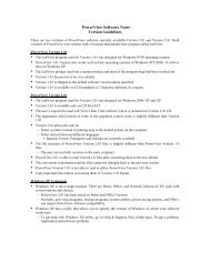
Visible differences between Versions 1.01 and the higher versions include:
• The appearance and location of some graphical control icons.
• Added features such as language and printer selection on version
2.01 and higher. Version 2.02 and higher includes improved
communications, ‘Save File’ prompt when exiting, and additional
COM ports to support Windows XP.
If PowerView is already installed on your computer, the version that you
are running can be found:
• On the original installation CD's.
• While in PowerView, by selecting About PowerView from the
HELP pull-down menu on the top.
Microsoft Corporation has created many versions of the Windows operating
system and associated products. The Windows XP platform has many
versions available depending on your computing and networking needs.

NOTE: PowerView is tested on different computers with different versions
of Windows, but we cannot duplicate all conceivable setups, options, and
types of programs. Whether or not PowerView will run completely and
successfully on your particular computer depends on several factors,
including the Windows platform and version, computer settings, user
settings, port settings, processor, network connections and network settings.
It is possible that software or equipment connected to the computer can
cause conflicts, and may need to be removed or settings need to be changed
in order to allow our radiometers to communicate with the program. At
times, for example, software used with Personal Digital Assistants (PDA’s)
can interfere with communication protocols.
File Conversion of PowerView Version 1.01 Files
The file structure for files created using PowerView Version 1.01 is slightly
different than higher PowerView versions. Higher versions above 1.01 are
able to read Version 1.01 files after converting them to the new format. The
conversion is permanent and the files cannot be changed back to the
previous version. PowerView Version 1.01 is not able to read or utilize
Version 2.01 or higher files.
NOTE:
Copy important files before converting them from Version 1.01, as they
will not be able to be read or utilized with Version 1.01 once converted.
Connecting the UV PowerMAP and UV Map Plus to PC
The UV PowerMAP and UV Map Plus can be connected to your PC via the
supplied USB Serial Port Adapter or via a serial COM port on your PC. EIT
Instrument Markets recommends that you use the supplied Keyspan USB
Serial Port Adapter to connect your instrument to the PC.
PowerView Software Installation
1. Load the PowerView Installation CD in an available drive.
2. From the Program Manager screen, click on the Start button.
3. Click on Run.

4. Click on Browse.
5. Select the drive where the Installation CD is located and double-click
setup.exe.
6. A RUN dialog box will appear with the path and file you selected.
Click on OK.
7. Follow the screen prompts to complete installation
USB Port Users
Install the Keyspan Software for your USB Serial Port adapter as per
manufacturer's instructions. Attach the supplied Interface Cable from your
PowerMAP or UV MAP Plus to the USB Serial Port Adapter. Connect the
USB Adapter cables to the USB port on your PC.
Serial COM Port Users
Attach the supplied Interface Cable to the serial COM Port to be used and
to the UV PowerMAP or UV MAP Plus.
Identifying and Setting COM Ports
1. Identify which COM port is designated in the Device Manager of
the Windows Control Panel, under System. USB Serial Port
Adapter users with Windows 2000 and XP can change the COM
port utilized. (For more detailed instructions for USB connection
users, refer to Appendix B on how to locate, identify, or change
the designated COM port).
2. In the “PC Setup” section Of PowerView, set the Port Number by
scrolling up or down, or overwrite the current entry to match the
port designated on your PC.
3. Scroll up or down to select the Baud Rate in kilobits per second
(the default baud rate likely does not need to be changed).
4. Click on the SAVE button in the PC Setup section to store these
settings.

Setup and Setup View
The UV PowerMAP and UV MAP Plus are configured at the factory prior
to shipping. These settings can be changed so the user can configure the
radiometer for their application. The sampling rate, active UV bandwidths,
and other features can be adjusted in this menu. The Setup view can be
found by selecting it from the TOOLS pull-down menu on the top. It is
divided into sections as shown in Figures 5 and 6.
Start the PowerView program and select SETUP from the TOOLS pulldown
menu to continue with setup and configuration.
Map Configuration
Figure 5. Setup View
1. The GET CONFIG button retrieves the radiometer’s current
configuration. Each enabled UV channel button will appear green,
disabled ones will appear gray. The UV Sample Rate is also
displayed.
2. To change which channels are enabled, click on each channel’s
button to turn it on or off. For the UV MAP Plus, only one channel
can be enabled. Verify that the correct channel is enabled
according to the calibration label on the unit.

3. To change the UV Sample Rate, click on the scroll buttons to the
left of the box or click on the box and select the desired rate. The
UV Sample Rate selected will determine the amount of time that
the PowerMAP/Map Plus is available to collect data. PowerView
automatically calculates and displays the resulting sample period.
Faster sample rates collect information that is more detailed but
also create larger files. Additional discussion on sample rates is
found in the "Sample Rates" section on page 35.
4. The THRESHOLD SETTINGS section gives the option of turning
the Start Threshold on or off and setting the temperature limit for
the Over Temp alarm. The Start Threshold is used when the
operator does not want the unit to trigger on low-level UV light. It
acts as a delay for an application that has a long distance between
the beginning of the process and the first UV source. The Over
Temp (C) sets the temperature at which the internal overtemperature
alarm will trigger.
5. Click on the SAVE CONFIG button to store the Map
Configuration. The Settings will not be saved unless the SAVE
CONFIG button is clicked.
Map Clock
This section defaults to and displays the clock settings of the PC. This clock
is used to time and date stamp the unit’s readings. This feature is useful
when tracking systems over time.
1. To manually set the radiometer’s clock, toggle the PC CLOCK
button to MANUAL, and enter the clock settings directly.
2. Store the settings in the radiometer by clicking on the SET MAP
CLOCK button.
Map Status
Click on the GET STATUS button to retrieve the unit’s information and
data configuration. In the window under the GET STATUS button you will
find:
“Collection Unit:” lists the type, firmware revision level and serial number
of the UV Data Collector (UDC).

“Optics Unit:” lists the same information about the Optics Head (DOB) and
includes the available channels.
“Data Config:” lists the sample rate setting (Hz) and the enabled channels.
“Start:” shows the unit’s date and time settings, its internal temperature and
its battery voltage. This information is also shown under the window.
PC Communication Errors
If your UV PowerMAP or UV Map Plus does not respond to PowerView
commands, refer to the Troubleshooting Communication Errors section in
Appendix C for possible errors.
Language
Versions 2.01 and higher of PowerView allows the user to select a language
other than English for the button names and icons. Language choices other
than English include Spanish, French, Portuguese, and German. Once a
new language has been selected, press SAVE. The PowerView program
will restart in order for the language to become the default language choice.
Figure 6. Language Selection

Basic Operation
After the radiometer is configured for the run, it is disconnected from the
PC, then exposed to the UV environment just as the actual product would
be. Descriptions of the pushbutton operation, audible alarm, and LED
indicator are given to aid in equipment familiarization.
Pushbutton Operation
A single pushbutton on the unit acts as the main operating switch. Its
operation is based on pressing it for a short or long period.
A short press turns the unit on and puts it in standby.
A second short press resets the unit, clears any stored data, and then puts
the unit in its run mode.
A long press will turn the unit off.
Audible Alarm
The audible alarm gives the operator audio feedback to register button
presses and error conditions.
Each time the pushbutton is pressed, the audible alarm will give a short
“beep”.
When the pushbutton is pressed and held, the audible alarm will beep
longer and stop. When the beep stops, the pushbutton is released.
The audible alarm will “chirp” once approximately every five seconds to
indicate a low battery condition. Re-charge the batteries as described later
in this manual.
The audible alarm will beep approximately once every 1.5 seconds to
indicate an over-temperature condition. (The alarm triggers when the unit’s
internal temperature exceeds 70°C). Allow the unit to cool prior to any
further use.

If the audible alarm beeps at a fast rate, an error has been detected. Contact
EIT Instrument Markets per the Warranty and Returns section of this
manual for further assistance.
LED Indicator
In standby mode, the LED will flash red at about one flash per second. The
period (time-on) of the LED indicates the memory fill status. As the
memory fills, the LED flashes at the same rate, but remains on for a longer
period. If the LED remains on, the memory is full.
When the unit is switched to run mode, the LED changes from red to green,
and continues to show the memory status.
If the LED flashes red or green at a constant, fast rate with the audible
alarm, an error has been detected. Contact EIT Instrument Markets per the
Warranty and Returns section of this manual for further assistance.
The Basic Data Run
From the standby mode, short-press the pushbutton to toggle the radiometer
into its run mode. Verify that the memory is not full.
1. Expose the radiometer to the UV source to be measured.
Ultraviolet Radiation
Although this product is not a source of UV light, it is used in a UV
environment. Refer to the UV source's documentation for
recommended protective measures against UV radiation present in
the UV environment.
2. Upon removal from the UV environment, short-press the button to put
the unit back into standby.
3. Connect the unit to the computer with the cable provided.

Transfer View
The run data is uploaded into the PowerView software through the Transfer
View screen. The Transfer View screen can be viewed by selecting
Transfer View from the VIEW pull-down menu on the top.
Uploading Data
Figure 7. Transfer View Screen.
1. Connect the unit to your PC.
2. From the VIEW pull-down list, click on TRANSFER. The Transfer
View screen will appear as shown in Figure 7.
3. Click on the BEGIN TRANSFER button to start the upload. The
transfer can be paused by clicking on PAUSE, or halted by clicking on
STOP. (Halting the transfer allows the data already transferred to be
stored). The TRANSFER STATUS, BYTES TRANSFERRED, TIME
REMAINING, and % COMPLETE show the transfer’s progress.
4. In the right side of the screen, click on the PREVIEW button to see a
preliminary view of the plot. A detailed look at the graph is available
once the transfer is complete in the Graph View screen.
5. The Unit Configuration and User Information is displayed in the
bottom right of the Transfer View screen. The Unit Configuration
loads in from the radiometer as part of the upload and cannot be edited.

6. User Information, such as UV system identification and test conditions,
can be entered at this time.
Graph View
After the plot is uploaded, it can be viewed graphically by selecting Graph
View from the VIEW pull-down menu on the top.
Figure 8. Graph View Screen
Viewing the Data in Graph Format
In the Graph View screen, the display of the UV channels and temperature
can be toggled on or off as desired.
The Sample and Reference buttons in the upper left of the screen control
which active channels (channels that were enabled during the run) will be
displayed. Clicking on these buttons toggles the display of their respective
channels.
The table in the upper right corner of the screen lists the channels that were
enabled for the run. Disabled channels are listed “N/A”.

To change the color and/or appearance of a trace in the plot, click on the
trace’s name in the upper right and choose the desired options from the
pop-up lists like shown below.
Figure 9. Channel Option Menu
Once the channels are set, click on the SAVE button to store the settings.
Click on the DEFAULT button to restore the trace options to the original
factory settings.
The SMOOTH ON/OFF button provides a filtering function to reduce
“noise” in the plot.
Click on the SMOOTH ON/OFF button to toggle it on or off. The button
color and name change to indicate whether this function is on.
Graph View Controls
An important feature of PowerView is the ability to simultaneously
compare two runs in its Graph View screen. The Graph View controls are
located under the graph area, and appear as shown in Figure 10. Scaling,
Zoom, Cursor, Plot Overlay, and Position are the major sections of the
Graph View controls. A list of their descriptions follows.

Scaling Zoom
Cursor
Plot Overlay
Position
Scaling Controls
Figure 10. Graph View Controls.
When a plot is transferred or opened, PowerView automatically sets the X
and Y axes to fit the plot in the viewing area. The first two pairs of controls
are used to scale and format these axes.
Auto Scale Sets the plot horizontally and/or vertically to
fit the entire plot in the viewable area. These
are used mostly for aborting zoom
functions.
X and Y Axis Scale Activates pop-up menu to change the
Format, Precision, or Mapping Mode of the
X or Y axis.
"Format" - Allows the user to change the presentation of the
axis numbering.
"Precision"- Sets the number of decimal places in the axis
numbering.
"Mapping Mode" - Scales the axes either linearly or
logarithmically.

Zoom Controls
(Default Settings Shown)
Figure 11. X and Y Scale Structure
These controls are accessed in a pop-up activated by the Zoom control.
Zoom Activates pop-up menu to select zoom
functions. The types of zoom functions are:
area, horizontal, and vertical zoom; undo
zoom; and zoom in and out. When a zoom
function is selected, the mouse pointer will
change to a magnifying glass.
To use the first three types of zoom, select
the type desired, then click and drag the
pointer to define the zoom area (dashed
lines will border the area). The zoom occurs
when the mouse button is released.
“Undo Zoom” undoes the last zoom
performed.
The remaining two functions provide
repeated zooming in or out, respectively.

Area
Undo Zoom
Position Controls
Figure 12. Zoom Controls
The operator can move the plot through the viewing area using the Plot
Position control.
Plot Position When selected, the pointer changes to a
hand. Click and drag the pointer to move the
plot across the viewable area.
Cursor Controls
Horizontal
Zoom In
Vertical
Zoom Out
Cursor measurement helps the operator analyze run data by facilitating both
absolute and relative measurement.
Cursor When the Cursor control is active, the
pointer will appear as a crosshatch that
changes when placed on a cursor. Click and
drag the cursor to the location desired.
Cursor Name REF- The reference cursor.
SMPL- The sample cursor.

X Position Displays the horizontal coordinate of the
cursor. The user can overwrite the
coordinate to manually place the cursor.
Y Position Displays the vertical coordinate of the
cursor. The user can overwrite the
coordinate to manually place the cursor.
Fine Adjust On/Off Toggles the Fine Adjust control for the
cursor. A black box indicates the Fine
Adjust is enabled.
Cursor Option Activates pop-up menu to change the cursor
appearance, show/hide the cursor name, or
locate the cursor.
Figure 13. Cursor Menu Structure

Cursor Lock Activates pop-up menu to select free cursor
movement or to lock it to a plot or point.
When “free”, the cursor(s) can be placed
anywhere in the viewing area. To lock the
cursor to a plot or point, select the channel
to lock to from the list in the bottom of the
menu. Select Snap to point or Lock to plot.
The horizontal axis of the cursor will go to
the trace specified. The vertical axis of the
cursor will stay in place.
Figure 14. Cursor Lock Menu
Fine Adjust When enabled (see Fine Adjust On/Off,
above), the cursor(s) can be moved slightly
up or down, or side to side by clicking on
the appropriate diamond. When the Fine
Adjust is enabled for both cursors, it will
move them simultaneously.
Plot Overlay Controls
SYNC PLOTS The SYNC PLOTS button is used to overlay
two points in the plot area. It does this by
horizontally aligning the Reference and
Sample cursors. Move the cursors to the two

points to overlay, then click on SYNC
PLOTS. A pop-up will appear with two
options: “Adjust by x.xx Sec.” and “Reset to
0 Offset”. Click on “Adjust by...” to overlay
the Sample cursor on the Reference cursor.
Clicking on the “Reset to...” button reverses
this function.
Cursor Diff(s) The distance between the Reference and
Sample cursors. (-3.48 is an example)
Overlaying Plots
Overlaying plots is demonstrated in Figure 15. Move the cursors to the two
points to overlay. In this example, the UV(A) (sample) and REF(A)
(reference) cursors are both placed on their respective curve's peaks.
Click on SYNC PLOTS. A pop-up box will appear with two options:
"Adjust by 7.96 Sec" and "reset to 0 offset". Note that the "7.96" seconds is
shown in the "Cursor Diff(s)" box and is unique to this example.
Click on "Adjust by 7.96 (example) Sec" to overlay the UV(A) and the
REF(A) cursors.
Click on the "Reset to 0 Offset" button to reverse the overlaying function.
Figure 16 shows the two plots being separated. Place the UV(A) cursor to
the right of the Sample trace (solid line) and the REF(A) cursor to the left
of the Reference trace (dashed line).
Click on SYNC PLOTS and click on "Adjust by -9.33 (example) Sec".
When the UV(A) cursor moves left and the REF(A) cursor moves right, the
traces are shifted outward and can be viewed individually.
NOTE: The numbers referred to are applicable to this example.

Figure 15. Overlaying Two Traces
Figure 16. Separating Two Traces

Sample and Reference Blocks
The upper block of the Sample section shows the unit identification and
certain test conditions for the sample plot. First, it lists the Collection Unit
name, firmware revision, and serial number. Secondly, it lists the same
information for the Optics Unit plus the UV channels installed in it. Next,
the Data Configuration gives the sample rate and which UV channels were
enabled for the run. Lastly, the start date and time stamp for the run is
displayed, along with the unit’s internal temperature and battery voltage.
All the information in this part of the Sample section is automatically
generated by the unit and cannot be edited.
The upper block of the Reference section shows the unit identification and
certain test conditions for the reference plot. First, it lists the Collection
Unit name, firmware revision, and serial number. Secondly, it lists the same
information for the Optics Unit plus the UV channels installed in it. Next,
the Data Configuration gives the sample rate and which UV channels were
enabled for the run. Lastly, the Start date and time stamp for the run is
displayed, along with the unit’s internal temperature and battery voltage.
All the information in this part of the Reference section is automatically
generated by the unit and cannot be edited.
The lower Sample and Reference blocks can be edited and used by the
operator to add comments such as lamp settings, line speed, materials used,
or lot numbers to the data file.
Data View
Figure 17. Sample and Reference Blocks
The Data View screen displays the UV and temperature readings for the
active channels numerically. The Data View screen can be viewed by
selecting Data View from the VIEW pull-down menu on the top. It has five

main sections- Total Energy Density, Peak Power Density, a section
containing Smooth, Cursor, and Threshold controls, and Sample and
Reference blocks (as described on p. 27).
Total Energy Density
Figure 18. Data View Screen
The Total Energy Density readings are shown in Joules/cm 2 . These
readings represent the calculation of power density over time- the
mathematical integral under the plot curve. The Average Temperature is the
mathematical integral under the temperature curve.
1. Click on the J/mJ button to toggle between Joules/cm 2 and
milliJoules/cm 2 .
2. Click on the C/F/K button to change the Average Temperature scale
between Celsius, Fahrenheit, and Kelvin scales.
3. The Sample, Ref., Diff., and % Diff. columns list the energy densities
and temperature for the sample plot and reference plot, the numerical
difference between them (Sample - Reference = Difference), and the
Difference as a percentage ([Sample ÷ Reference] X 100 = %Diff.).
PowerView does not calculate the %Diff. for Peak Temperature).

Peak Power Density
The Peak Power Density readings are shown in Watts/cm 2 . These readings
represent the peak irradiance of each channel measured. The Peak
Temperature is the highest temperature recorded for the run.
1. Click on the W/mW button to toggle between Watts/cm 2 and
milliWatts/cm 2 .
2. Click on the C/F/K button to change the Peak Temperature scale
between Celsius, Fahrenheit, and Kelvin scales.
3. The Sample, Ref., Diff., and % Diff. columns list the peak power
densities and temperature for the sample plot and reference plot, the
numerical difference between them (Sample - Reference = Difference),
and the Difference as a percentage ( [Sample ÷ Reference] X 100 =
%Diff.). PowerView does not calculate the %Diff. for Peak
Temperature.
Smooth On/Off
The Smooth On/Off control provides a filtering function to reduce “noise”
in the plot. The control’s name and color change to indicate whether the
function is on or off.
Cursors On/Off
The Cursors On/Off control toggles the cursors on for measurement
between where the cursors are set.
The two boxes to the right of the Cursors control show the horizontal (X)
coordinates of the Reference (REF) and Sample (SMPL) cursors. When the
cursors are turned on, the measurement data is limited to the section of the
plot that is bound by the cursors. This is useful in measuring the total
energy density of one lamp in a multiple-lamp system.
Figure 19 shows the cursors being used for comparing the peak power
densities of two different runs.

Figure 19. Peak Comparisons (Graph View and Data View)
With the UV(A) and REF(A) cursors on their respective peaks, the
difference between the two peaks can be seen in the Y Coordinate boxes
(0.474 and 0.455 for this example).
To see the measurement more accurately, go to the Data View Screen by
selecting it from the VIEW tab above. With the cursors on, the Total
Energy Density, Peak Power Density and Temperature readings are taken
from between the cursors. Note that the Peak Power Density of the Sample
trace is about the same as the Y-coordinate of the UV(A) cursor. The same
is true for the Reference trace and REF(A) cursor. The "Diff" column
shows the difference between the readings.
Figure 20, on the next page, shows the UV(A) cursor locked to the sample
UV(A) trace. The Reference traces are off, so the REF(X) cursor is labeled
OFF. The Peak Power Density is at the OFF cursor, the highest point
between the cursors. In Figure 21, the cursors are on either side of the
peak. The Peak Power Density is no longer at the OFF cursor's position, but
the Total Energy Density is still taken from between the cursors. The Peak
Power Density is now the highest point on the trace.

Figure 20. Cursor Measurement (Graph View and Data View)
Figure 21. Cursor Measurement (Cursors on either side of a peak)

Threshold On/Off
The Threshold On/Off control turns the threshold function on or off. When
the Threshold is off, the entire plot, including any negative excursions, is
tabulated.
When the Threshold is on, it can be adjusted using the Threshold (mW)
control to the right. Type in the threshold desired or click on the
increment/decrement arrows on the left side of the box.
NOTE: There is a difference between Threshold Off and a “0” Threshold.
When the threshold is off, everything is calculated. When the threshold is
on, but is set to 0.00, only data with positive values are used in calculations.
The figures below demonstrate how the Threshold function works. The
shaded areas in both figures represent where data is collected with the
Threshold set at 5mW and 10mW respectively.
0.035
0.030
0.025
0.020
0.015
0.010
0.005
0.000
-0.003
Figure 22. Graph View With Threshold at 5mW
0.035
0.030
0.025
0.020
0.015
0.010
0.005
0.000
-0.003
Figure 23. Graph View With Threshold at 10mW

Manipulating Files in PowerView
Clicking on the FILE button opens a pull-down list with the following
selections: OPEN, CLOSE, SAVE, EXPORT, PRINT, and EXIT.
Opening Files
When OPEN is selected, a pop-up will ask whether to open the file as a
sample or reference plot. Check the appropriate box or click on Exit to
abort.
If the operator wants to see a different file as the Sample or Reference file,
the operator can open a file on top of the one to be changed. The “new” file
is displayed and the other file is closed.
NOTE: A run must be saved as a file before a file is opened on top of it.
Otherwise, the run data will be lost.
Closing Files
To close a file, click on CLOSE. A pop-up will ask which file to close (the
sample or reference). Select the appropriate box or click on Exit to abort.
A run must be saved as a file before closing it or the run data will be lost.
Saving Files
To save a run as a file, click on SAVE. A pop-up will ask whether to save
the run as a sample or reference file.
Check the appropriate box or click on Exit to abort.
Enter a name for the file before the numeric suffix. (The suffix
appears as “_x” where x is a number that automatically
increments with each file save on that day).

Exporting Files
Files can be exported into spreadsheets from PowerView as follows.
1. Click on the FILE pull-down menu and select Export.
2. A File Export dialog will appear. Select which file (Sample or
Reference) to export. An Enter Filename dialog will appear.
3. Select a location for the file.
4. PowerView defaults to the file's current name. It can be changed if
desired. If the file already exists, you will be prompted whether to
overwrite the existing file.
5. PowerView also defaults to a Custom Pattern (*.txt) file type. Do not
change the file type.
6. Click on Save. The data run file is now a tab-delimited text file, which
can be imported into a spreadsheet program.
Printing Data
Click on PRINT to print the current screen to your active default printer.
Exiting PowerView
Save any data runs before exiting. Version 2.02 and higher will prompt you
to “Save File” when exiting. When using Version 2.01 or lower, remember
to save your data runs before exiting, otherwise, they will be lost.. Click on
EXIT to close the PowerView application.
Basic Applications
Evaluating UV Lamp Output
The trace in the Graph View screen allows you to compare the peak UV
irradiance of each lamp in a multi-lamp curing system. If you expect
similar peak intensities from each bulb in a multi-lamp system, you will be
able to clearly see when one bulb is not outputting at the same rate as the
others. The PowerView software allows you to save the information from
a lamp system when the bulbs are new and the reflectors are clean as the
reference for comparison to a later sample. UV PowerMAP allows you to

profile and compare the output in the four spectral channels that it
measures. UV MAP Plus does the same on one specific channel.
Focusing Lamps
The shape of the trace in Graph View is indicative of whether or not the
lamp is focused. A non-uniform or jagged curve indicates that the lamp is
not physically located at the focus of the reflector. The trace will also allow
you to compare reflector materials, reflector shapes and wavelength specific
degradation over time and to other systems.
Monitoring Temperature
Many substrates and compounds used in UV curing will deteriorate or
undergo physical change when subjected to excessive temperatures. High
infrared temperatures accompany the UV in many curing systems.
Temperature measurement will help you maintain the balance of getting the
necessary amount of UV while not exceeding the temperature range of the
product. Temperature results from the thermocouple are best utilized if the
thermocouple can be placed on the same plane as the optical window on the
Optics Head.
Discussion on Sample Rates
NOTE: This discussion uses the UV PowerMAP as an example. Comparisons
for the UV MAP Plus can be drawn from this discussion as well.
Technological improvements allow the UV PowerMAP to sample much faster
and store more information than radiometers designed just a few years ago.
Earlier EIT Instrument Markets radiometers had sample rates of up to 160
samples per second and could store a maximum of 6000 UV and temperature
data points. The UV PowerMAP has a maximum sample rate of 2048 samples
per second and can store up to 180,000 data points in its memory.
In the PowerView Setup screen, the user can enable or disable any of the four
UV channels in the PowerMAP (A, B, C, and V). The user can also select UV
sample rates from 128 to 2048 samples per second. As the channels and
sample rates are set, the maximum sample time available is displayed in

minutes. Faster sample rates and more enabled channels will decrease the time
available to take data. With the fastest sample rate set and all four channels
enabled, the maximum sample time is 1.4 minutes.
Higher sample rates will cause some differences in readings. First, the
increased number of instantaneous measurements yields a higher integral
resolution. The measurement curve is sharper and more defined. This increase
in resolution will likely result in a reading slightly higher than a reading taken
with a radiometer having a slower sampling rate. Secondly, the peak
irradiance is more accurately measured. The variance when measuring peak
irradiance lies in the sample rate versus the time spent under the focal point of
the lamp. Table 2 shows the comparison between EIT Instrument Markets'
UV Power Puck (at 25 samples per second) and a PowerMAP sampling at
1024 and 2048 samples per second. For the purpose of this comparison, we
assume that the UV lamp has a 3/4-inch focal plane and that the conveyor
speed is a constant 10 meters per minute. Similar calculations can be made for
any system if the conveyor speed and the focal plane are known.
Calculation Power Puck @
25 S/s
Conversion from 10m/minute =
m/min to in/sec 6.5 inches/second
Samples/inch 25 samples ÷ 6.5 in.
unit can measure
= 3.85 samples/in.
Samples
measured under
the focal plane
PowerMAP @
1024 S/s
10m/minute =
6.5 inches/second
1024 samples ÷ 6.5 in.
= 157.54 samples/in.
PowerMAP @
2048 S/s
10m/minute =
6.5 inches/second
2048 samples ÷ 6.5 in.
= 315.08 samples/in.
3.85 x 0.75 = 2.88 157.54 x 0.75 = 118.16 315.08 x 0.75 = 236.31
Table 2. Sample rate comparisons.
Another difference with a higher sample rate appears in the Graph View of
the system profile. Some UV lamp systems have power sources that cycle the
lamps on and off many times per second. The PowerMAP can actually detect
and record this cycling. To reduce the effects of this sensitivity on the plot,
the Graph View screen contains a SMOOTH BUTTON. The SMOOTH
BUTTON filters and minimizes these effects to make the profile more
readable.

Maintenance
The user should perform routine maintenance. It consists of battery charging,
cleaning, removing/installing the Optics Head, and returning the unit for
calibration.
Battery Charging
1. The PowerMAP and UV MAP Plus instruments are supplied with
a universal 100-240VAC, 50/60 Hz switching power supply
(charger), and 4 interchangeable input plug adaptors that securely
lock into position and quickly release by depressing the adaptor
button.
2. Insert the charger’s plug into the UDC’s charging jack.
3. Attach the country specific plug adaptor to the power supply, and
insert into an AC outlet.
WARNING!
Risk of electric shock. Make certain that the AC outlet is the correct
voltage and configuration for the charger. Personal injury and/or
damage to the unit may occur if the voltage is incorrect.
Cleaning
4. Allow the radiometer to charge for 1 hour.
To clean the optical surfaces, refer to the Cleaning Instructions provided in
the Appendix.
To clean the case of the radiometer, use a soft cloth and isopropyl alcohol.
For the Thermocouple probe tip, use a soft cloth with acetone if needed.

Optics Head Removal and Installation
ESD Sensitive Device
The gold pins on the Optics Head connect directly to circuitry that is
sensitive to electrostatic discharge. Personnel should follow proper ESD
handling procedures when installing or removing the Optics Head.
1. TURN OFF THE UV DATA COLLECTOR (UDC) PRIOR TO
REMOVING OR INSTALLING THE OPTICS HEAD. Press and hold
the pushbutton until the UDC turns off.
2. Using the 1/16” hex driver provided, loosen the set-screws in the sides
of the UDC.
3. Carefully pull the Optics Head off the UDC.
4. Put the Optics Head in the transport case provided or equivalent ESDsafe
packaging for storage or transportation.
5. To re-install the Optics Head, align its mechanical alignment pins with
their holes in the UDC.
6. Making sure that all of the gold pins are aligned with their respective
holes, push the Optics Head and the UDC together.
7. Re-tighten the set screws.
Calibration
EIT Instrument Markets recommends that the Optics Head be calibrated
every six months. The calibration expiration date can be found in two
places:
1. It is located on the calibration label on the optics head.
2. It is displayed on the Certificate of Calibration under Calibration Results
as Next Calibration Due: [Date Inserted]
Only the Optics Head needs to be returned for calibration. Refer to the
"Returning the Instrument to EIT Instrument Markets" section, for
instructions on how to ship your unit to EIT-IM for calibration.

Standard Accessories
These accessories are included with a UV PowerMAP or UV MAP Plus set.
1. PowerView Software CD
2. Universal Battery charger, 110-240 VAC, 50/60 Hz, with plug adaptors
5. Computer interface cable
6. Serial-to-USB adaptor with software CD
4. Thermocouple probe
5. Carrying Case
6. User's Manual
7. Optics Head Transport Case
8. Hex key
Optics Heads and standard accessories are available for individual sale.
Contact EIT Instrument Markets or an EIT Instrument Markets authorized
representative for ordering information.
Specifications
Electrical Specifications
Configuration
UV Ranges
2 Part: Detachable Optics Head and UV
Data Collector
Optics Head: Supports optics to measure 4
spectral regions
UDC: 256 bytes non-volatile memory
High Power: 200mW to 20W (UVA,
UVB, UVV ) ; 20mW-2W ( UVC)
Low Power: 2mW to 200mW (UVA,
UVB, UVV) ; 1mW to 100mW (UVC)
Spectral Response UVA (320-390nm), UVB (280-320nm),
UVC (250-260nm), UVV (395-445nm)
UV Accuracy +/-5% typical, +/- 10% maximum
Temperature Measurement Type J; Input Range: 500 o C Maximum
(Thermocouple range determined by
thermocouple wire used); Sample rate: 32
samples per second
UV Sample Rates User-adjustable from 128 to 2048 samples
per second

UV Sample Period Maximum of 1 hour, determined by
configuration
Operating Temperature Range 0-70 o C; over-temperature alarm @ 65 o C
Unit Operation One Push Button Switch
Indicators
One Single Tone Audible Indicator
Dual-Color LED (Red/Green)
Battery Nickel Metal Hydride (NiMH)
Battery Cycles 500 typical
Charging Period 1 hour quick charge at temperatures below
35 o C
Universal Charging Adapter AC input: 100-240VAC, 50/60Hz. 12 VDC
@ 250 mA
Operating Time Determined by configuration. Guideline:
four channels on @ 512 Samples/ second
for a 2-minute sample period yields 30+
readings on one charge.
Communication to PC
Format RS232 Serial Port
Speed 9600 to 115k baud
PowerView Software
Minimum Computer
Requirements
Pentium 60MHz, 16MB RAM, one serial
port, one parallel port; 20MB space
available on hard drive; CD-ROM drive;
Windows 95 operating system
Interface Windows-based fully graphical interface
Mechanical Specifications
Unit Dimensions 3.50”W X 9.0”L X 0.5”D (8.89cm X
22.86cm X 1.27cm)
Weight 20.2 ounces (570 grams)
Materials Aluminum chassis with stainless
steel covers
Table 3. Electrical and mechanical specifications (subject to change).

Spectral Response Curves
The Spectral Response Curves for the four UV channels are shown in
Figure 24 below. The UV PowerMAP has all four channels, the UV MAP
Plus has only one channel.
300 325 350 375 400 425
Wavelength (nm)
UV-A
230 240 250 260
270
Wavelength (nm)
UV-C
Figure 24. Spectral Response Curves.
250 275 300 325 350 375
Wavelength (nm)
UV-B
375 400 425 450
Wavelength (nm)
UV-V

Optics Locations
The locations of the optics for each UV channel are shown in Figure 25.
The UV PowerMAP has all four channels, the UV MAP Plus has only one
channel.
B C
A V
Warranty and Returns
New Product Warranty
Top
Optics Head
Figure 25. UV Channel Locations.
EIT Instrument Markets warrants that all goods described in this manual
(except consumables) shall be free from defects in material and
workmanship. Such defects must become apparent within six months after
delivery of the goods to the buyer.
EIT Instrument Markets' liability under this warranty is limited to replacing
or repairing the defective goods at our option. EIT Instrument Markets shall
provide all materials and labor required to adjust, repair, and/or replace the
defective goods at no cost to the buyer only if the defective goods are
returned, freight prepaid, to EIT Instrument Markets during the warranty
period.
EIT Instrument Markets shall be relieved of all obligations and liability
under this warranty if:

1. The user operates the device with any accessory, equipment,
or part not specifically approved, manufactured, or specified
by EIT Instrument Markets, unless the buyer furnishes
reasonable evidence that such installations were not a cause of
the defect. This provision shall not apply to any accessory,
equipment, or part that does not affect the proper operation of
the device.
2. Upon inspection, the goods show evidence of becoming
defective or inoperable due to abuse, mishandling, misuse,
accident, alteration, negligence, improper installation, lack of
routine maintenance, or other causes beyond our control.
3. The goods have been repaired, altered, or modified by anyone
other than EIT Instrument Markets authorized personnel.
4. The buyer does not return the defective goods, freight prepaid,
to EIT Instrument Markets within the applicable warranty
period.
There are no warranties that extend beyond the description on the face
hereof. This warranty is in lieu of - and is exclusive of - any and all other
expressed, implied, or statutory warranties or representations. This
exclusion includes merchantability and fitness, as well as any and all other
obligations or liabilities of EIT Instrument Markets. EIT Instrument
Markets shall not be responsible for consequential damages resulting from
malfunctions of the goods described in this manual.
No person, firm, or corporation is authorized to assume for EIT Instrument
Markets, any additional obligation or liability not expressly provided for
herein except in writing duly executed by an officer of EIT Instrument
Markets.
If any portion of this agreement is invalidated, the remainder of the
agreement shall remain in full force and effect.
This warranty shall not apply to any instrument or component not
manufactured by EIT Instrument Markets.

Calibration and Repair Warranty
EIT Instrument Markets will warranty calibration and/or repair services just
performed, for 90 days. This Calibration and Repair Warranty does not
apply to nor cover repairs that may otherwise occur to the instrument. Such
repairs may be covered under the New Product Warranty based on the age
of the instrument.
Returning the Instrument to EIT Instrument Markets
1. Warranty Repair:
Contact EIT Instrument Markets before returning your unit for
warranty repair. An RMA is not required.
When returning the equipment under warranty, include the cabling,
software, and charger sent with the equipment so that EIT Instrument
Markets can evaluate the system.
Please return the equipment in the original (or equivalent) packaging.
You will be responsible for damage incurred from inadequate
packaging, if the original packaging is not used.
The customer is responsible for insuring the unit during
transportation to EIT Instrument Markets.
Equipment repaired under warranty will be returned to the user with no
charge for the repair or shipping. EIT Instrument Markets will notify
you of repairs not covered by warranty and their cost prior to
performing any work on the equipment.
EIT Instrument Markets reserves the right to make changes in design at
any time without incurring any obligation to install the same on units
previously purchased.
2. Non-Warranty Repair or Instruments Returned for Calibration:
You do not need to contact EIT Instrument Markets before returning
your unit for repair or calibration. An RMA is not required.

Please return the equipment in the original packaging (or equivalent)
to the address provided below (Specify "Non-Warranty Returns
Department"). You will be responsible for damage incurred from
inadequate packaging, if the original packaging is not used.
The customer is responsible for insuring the unit during
transportation to EIT Instrument Markets.
EIT Instrument Markets will contact you with the needed repairs and
the cost of repair before service begins. Repair service on calibrated
units includes calibration.
Address for Returning All Instruments to EIT-IM
Ship the unit, freight prepaid, to the address below:
EIT-IM
108 Carpenter Drive
Sterling, VA 20164 USA
Attention: Returns Department
Include your company name, address, telephone number, fax number, and
e-mail address on your shipping documents. EIT Instrument Markets will
contact you if any additional information is needed.

Appendix A
Optics Cleaning Instructions
The following guidelines are for cleaning the optical surfaces on EIT
Instrument Markets instruments. However, EIT Instrument Markets cannot
have full knowledge of contaminants present in all applications and as a result
cannot test for their effects. Therefore, we cannot assume responsibility for
damage to customer instruments, which results from following these
directions once the warranty period has expired. Also, customers are advised
to obtain and read the MSDS for any chemical used for cleaning optics, and
for taking necessary precautions. EIT Instrument Markets makes no claim for
the safety of any of these chemicals.
1. LOOK.
Closely examine the optical surface. If no contaminant is visible, it is best not
to clean the instrument. The optics are delicate and handling should be
minimized. The two exceptions to this rule are when:
a.) It is known that a process chemical has come in contact with the
instrument's optics, or
b.) A shift in readings has been observed with the instrument, and the design
of the UV system is such that contamination of the radiometer is a
possible cause of the measurement error.
2. BLOW.
The next step is to use compressed gas to remove any loose material from the
surface of the optics. This step is necessary because loose material, especially
silicates and other abrasive components, can cause scratching of the optical
surface during the remaining steps. Compressed gasses we recommend, in
order of preference, are:
(a) Dry nitrogen
(b) Chemtronics® Duster (p/n's ES1017, ES1217, ES1617) or similar
tetrafluoroethane-based products
(c) A rubber air bulb (typically found in camera supply shops)
(d) Compressed air from an oil-free, instrument grade system, sometimes
referred to as instrument air

In the case of any compressed gas, it is best to avoid making the optic too
cold. The resulting condensation, while typically easy to remove, presents
added difficulty in the cleaning process.
Two common practices are not recommended. Blowing on the optics with the
mouth is not recommended; various components of saliva are extremely
difficult to remove from the optics. Ordinary compressed air (sometimes
referred to as shop air) should also be avoided because of the difficulty in
removing oil from the optical surface.
3. FLOOD.
Apply a liberal amount of solvent to the window. The purpose of the solvent
is to loosen the contaminants from the surface, so surface tension can remove
the contaminant in step 4. The solvents used depend on what the user has
available, and what contaminants are expected in the field. EIT Instrument
Markets recommends cleaning the optic once with isopropyl alcohol, and
once with acetone for best results. Other suitable solvents include de-ionized
water, methyl alcohol, and ethyl alcohol. Customers working with non-polar
chemicals may find Methyl-ethyl-ketone (MEK) to be an effective solvent.
Customers should avoid using solutions containing detergents.
4. WIPE
Using a lint-free wipe or a cotton swab, wipe the surface clean. Either the
wipe or swab needs to be thoroughly wet with the solvent, so the surface
tension of the solvent will allow the contaminant to be captured on the wipe.
Users may find it convenient to start again at step 3 with a second solvent. A
source for lint free wipes is Kimberly Clark, Inc.'s Kimwipes.
EIT Instrument Markets does not recommend wiping the surface with a dry
wipe or swab of any kind. The absence of solvent greatly increases the
chance for the optical surface to be abraded.
EIT Instrument Markets can provide cleaning advice, assistance, and repair or
replacement in cases where these guidelines fail to remove contaminants.
Following these guidelines will help customers get long life and accurate
readings from their radiometers.

Appendix B
Locating, identifying, and changing the Keyspan COM port
in Windows 2000 and XP Operating Systems.
1. Go to the Start Menu.
2. Click on Control Panel.
3. Windows 2000: Click on “System” Icon.
Windows XP: Click on “Performance and Maintenance”. Or, in Classic
Mode, click on the “System” Icon from the Control Panel window.
4. The System Properties Window will appear.
5. Click the Hardware tab.
6. Click on Device Manager.
7. Click on + Ports (COM and LPT). The active COM Port will be
identified here, for 2000 and XP users, continue with Step 8 to
change COM port.
8. Double-click Keyspan USB Serial Port (COM4)
9. Click on Keyspan USB Serial Port (COM4) Properties.
10. Click on Port Settings.
11. Click the Start Assistant button.
12. The Keyspan USB Serial Adapter Assistant window will appear.
13. Click on Port Mapping.
14. Click on the drop down box next to "COM port mapping for selected
adapter port".
15. Select COM5 (or higher)
16. A window will pop up asking: "Keyspan Serial Adapter - COM Port
name setting change. Do you want to continue?" Click YES.
17. A window will pop up: "Keyspan Serial Adapter - COM Port Remap.
The Port Remapping request succeeded." Click OK.
18. The Device Manager and the Keyspan USB Serial Port Properties
window will now display the COM Port selected.
19. Close all Keyspan Windows and the Device Manager and Control Panel
windows.
20. Open PowerView Software (21026).
21. Click on Tools, then click Setup.
22. Click on PC Setup.
23. Set Port Number to the same number as the COM Port selected above.
24. Click SAVE.

Appendix C
Troubleshooting Communication Errors
Sample PC Error Prompt
Common Communication problems are Errors 37, 38, and 5000. Errors 37
and 38 indicate a serial port conflict or incorrect port selected. Error 5000
indicates communication has failed. Follow the instructions below to
troubleshoot any communication error.
1. Ensure that the battery of the unit is charged.
2. Check all communication cable connections.
3. Confirm that the COM port designated by your PC matches
the COM port selected in PowerView.
4. If using the USB serial adapter, ensure the adapter software
has been installed per the manufacturer's instructions.
5. In PowerView, Tools, Set-up, slow the Baud Rate
settings down to see if the slower speeds allow
communication. Try adjusting the Baud Rate one
step at a time. See the reference on the right.
6. If you are still unable to communicate, on your computer,
click on the Advanced Tab on your Communications Port
Properties Window and adjust the Transmit and Receive
Buffers to the lowest setting.

7. Communication to and from your radiometer was checked
during calibration at EIT Instrument Markets. If you are still
having problems, try communicating with the unit on another
computer, preferably one without potential conflicts from
networks or other devices such as PDA’s.
8. Windows XP contains a utility that allows you to specify the
version of Windows in which your software best performs.
For more information, click the Start button and click Help
and Support. In the Help and Support Center window under
help topics, click Fixing a Problem. Then click Application
and software problems. Select the task you are attempting.
Other Errors
Other common errors users may experience are Error 71 and 8.
Error 71 is a result of opening a Version 2.01 or higher file version of
PowerView with Version 1.01.software. Ensure that you have safely
converted the file (instructions on p.10) to view in a newer version of
PowerView.
Error 8 is a file permission error resulting from the "read-only" attribute
being selected. To reset this attribute, open Windows Explorer and open
the folder that the .eit file is located in. Right-click on the file, select
properties, and ensure the "read-only" box is not checked.

Regulatory Statements
United States:
NOTE: This equipment has been tested and found to comply with the
limits for a Class A digital device, pursuant to part 15 of the FCC Rules.
These limits are designed to provide reasonable protection against
harmful interference when the equipment is operated in a commercial
environment. This equipment generates, uses, and can radiate radio
frequency energy and, if not installed and used in accordance with the
instruction manual, may cause harmful interference to radio
communications. Operation of this equipment in a residential area is
likely to cause harmful interference in which case the user will be
required to correct the interference at his own expense.
European Union Countries:
This equipment is a Class A device, suitable for use in all establishments
other than domestic and those directly connected to a low voltage power
supply network which supplies buildings used for domestic purposes.
This equipment is in conformity with the following standards and
therefore bears CE marking:
IEC 61326-1:2005
EN55011: 1998
EN61000-4-2: 1995, A1: 1998, A2: 2001
EN 61000-4-3: 2002, A1: 2002
following the provisions of the applicable directives:
98/34/EEC and amendments
89/336/EEC and amendments.
Designed and manufactured in the USA. Patent Pending.

Electronic Instrumentation & Technology, Inc.,
Instrument Markets Group
108 Carpenter Drive, Sterling, VA 20164 USA
Telephone: 703-707-9067 • Fax: 703-478-0815
www.eitinc.com
100200PWR Rev E