Quantum Mechanics Lecture Notes - Old Dominion University
Quantum Mechanics Lecture Notes - Old Dominion University
Quantum Mechanics Lecture Notes - Old Dominion University

You also want an ePaper? Increase the reach of your titles
YUMPU automatically turns print PDFs into web optimized ePapers that Google loves.
<strong>Quantum</strong> <strong>Mechanics</strong><br />
<strong>Lecture</strong> <strong>Notes</strong><br />
J. W. Van Orden<br />
Department of Physics<br />
<strong>Old</strong> <strong>Dominion</strong> <strong>University</strong><br />
August 21, 2007
Contents<br />
1 Introduction: The <strong>Old</strong> <strong>Quantum</strong> Theory 1<br />
1.1 Classical Physics . . . . . . . . . . . . . . . . . . . . . . . . . . . . . 1<br />
1.2 Thermodynamics and Statistical Physics . . . . . . . . . . . . . . . . 4<br />
1.2.1 Black Body Radiation . . . . . . . . . . . . . . . . . . . . . . 4<br />
1.2.2 The Photoelectric Effect . . . . . . . . . . . . . . . . . . . . . 6<br />
1.3 Atomic Physics . . . . . . . . . . . . . . . . . . . . . . . . . . . . . . 7<br />
1.3.1 Cathode Rays . . . . . . . . . . . . . . . . . . . . . . . . . . . 8<br />
1.3.2 Radioactive Decay . . . . . . . . . . . . . . . . . . . . . . . . 9<br />
1.3.3 The Bohr-Sommerfeld Model . . . . . . . . . . . . . . . . . . 11<br />
1.4 Wave Particle Duality . . . . . . . . . . . . . . . . . . . . . . . . . . 15<br />
1.4.1 Compton Scattering . . . . . . . . . . . . . . . . . . . . . . . 15<br />
1.4.2 Electron Diffraction . . . . . . . . . . . . . . . . . . . . . . . . 17<br />
2 Mathematical Background to <strong>Quantum</strong> <strong>Mechanics</strong> 19<br />
2.1 Vector Spaces . . . . . . . . . . . . . . . . . . . . . . . . . . . . . . . 19<br />
2.1.1 The Scalar Product . . . . . . . . . . . . . . . . . . . . . . . . 20<br />
2.1.2 Operators . . . . . . . . . . . . . . . . . . . . . . . . . . . . . 22<br />
2.1.3 Matrix Notation . . . . . . . . . . . . . . . . . . . . . . . . . 22<br />
2.1.4 The Eigenvalue Problem . . . . . . . . . . . . . . . . . . . . . 25<br />
2.2 The Continuum Limit . . . . . . . . . . . . . . . . . . . . . . . . . . 31<br />
3 The Schrödinger Equation 39<br />
3.1 Wave Particle Duality . . . . . . . . . . . . . . . . . . . . . . . . . . 39<br />
3.2 Wave Packets . . . . . . . . . . . . . . . . . . . . . . . . . . . . . . . 42<br />
3.3 The Schrödinger Equation . . . . . . . . . . . . . . . . . . . . . . . . 45<br />
3.4 The Interpretation of the Wave Function . . . . . . . . . . . . . . . . 47<br />
3.5 Coordinate Space and Momentum Space Representations . . . . . . . 49<br />
3.6 Differential Operators . . . . . . . . . . . . . . . . . . . . . . . . . . . 51<br />
3.7 The Heisenberg Uncertainty Relation . . . . . . . . . . . . . . . . . . 53<br />
3.8 Review of Classical <strong>Mechanics</strong> . . . . . . . . . . . . . . . . . . . . . . 56<br />
3.9 Generalization of the Schrödinger Equation . . . . . . . . . . . . . . . 57<br />
4 The Time-Independent Wave Function 61<br />
i
5 Solutions to the One-Dimensional Schrödinger Equation 67<br />
5.1 The One-dimensional Infinite Square Well Potential . . . . . . . . . . 71<br />
5.2 Bound States in a Finite Square Well Potential . . . . . . . . . . . . 80<br />
5.2.1 Parity . . . . . . . . . . . . . . . . . . . . . . . . . . . . . . . 87<br />
5.3 The One-Dimensional Harmonic Oscillator . . . . . . . . . . . . . . . 89<br />
6 Scattering in One Dimension 97<br />
6.1 The Free-Particle Schrödinger Equation . . . . . . . . . . . . . . . . . 97<br />
6.2 The Free Wave Packet . . . . . . . . . . . . . . . . . . . . . . . . . . 102<br />
6.3 The Step Potential . . . . . . . . . . . . . . . . . . . . . . . . . . . . 105<br />
7 The Solution of the Schrödinger Equation in Three Dimensions 111<br />
7.1 The Schrödinger Equation with a Central Potential . . . . . . . . . . 113<br />
7.1.1 Spherical Harmonics . . . . . . . . . . . . . . . . . . . . . . . 116<br />
7.2 The Radial Equation . . . . . . . . . . . . . . . . . . . . . . . . . . . 117<br />
7.3 Solution of the Radial Equation for a Free Particle . . . . . . . . . . 118<br />
7.4 The Finite Spherical Well . . . . . . . . . . . . . . . . . . . . . . . . 120<br />
7.4.1 Bound States . . . . . . . . . . . . . . . . . . . . . . . . . . . 121<br />
7.4.2 The Infinite Spherical Well . . . . . . . . . . . . . . . . . . . . 123<br />
7.5 The Coulomb Potential . . . . . . . . . . . . . . . . . . . . . . . . . . 124<br />
7.5.1 Degeneracy . . . . . . . . . . . . . . . . . . . . . . . . . . . . 127<br />
7.5.2 Radial Wave Functions . . . . . . . . . . . . . . . . . . . . . . 128<br />
8 Formal Foundations for <strong>Quantum</strong> <strong>Mechanics</strong> 131<br />
8.1 Review . . . . . . . . . . . . . . . . . . . . . . . . . . . . . . . . . . . 131<br />
8.2 Dirac Notation . . . . . . . . . . . . . . . . . . . . . . . . . . . . . . 135<br />
8.3 Heisenberg Representation . . . . . . . . . . . . . . . . . . . . . . . . 138<br />
8.4 Matrix Representation . . . . . . . . . . . . . . . . . . . . . . . . . . 140<br />
9 Symmetries, Constants of Motion and Angular Momentum in <strong>Quantum</strong><br />
<strong>Mechanics</strong> 143<br />
9.1 Translations . . . . . . . . . . . . . . . . . . . . . . . . . . . . . . . . 143<br />
9.2 Time Translation . . . . . . . . . . . . . . . . . . . . . . . . . . . . . 145<br />
9.3 Rotations . . . . . . . . . . . . . . . . . . . . . . . . . . . . . . . . . 146<br />
9.3.1 Rotations of a Vector . . . . . . . . . . . . . . . . . . . . . . . 146<br />
9.3.2 Rotations of Wave Functions . . . . . . . . . . . . . . . . . . . 149<br />
9.4 The Angular Momentum Operators in Spherical Coordinates . . . . . 152<br />
9.5 Matrix Representations of the Angular Momentum Operators . . . . 156<br />
9.6 Spin . . . . . . . . . . . . . . . . . . . . . . . . . . . . . . . . . . . . 161<br />
9.6.1 Spin 1/2 . . . . . . . . . . . . . . . . . . . . . . . . . . . . . . 162<br />
9.6.2 The Intrinsic Magnetic Moment of Spin-1/2 Particles . . . . . 164<br />
9.6.3 Paramagnetic Resonance . . . . . . . . . . . . . . . . . . . . . 166<br />
ii
10 Addition of Angular Momenta 171<br />
10.1 Introduction . . . . . . . . . . . . . . . . . . . . . . . . . . . . . . . . 171<br />
10.2 Addition of Two Angular Momenta . . . . . . . . . . . . . . . . . . . 172<br />
10.2.1 General Properties of Clebsch-Gordan Coefficients . . . . . . . 178<br />
10.2.2 Example: Addition of j1 = 1 and j2 = 1 . . . . . . . . . . . . 180<br />
11 Rotation Matices and Spherical Tensor Operators 183<br />
11.1 Matrix Representation of Rotations . . . . . . . . . . . . . . . . . . . 183<br />
11.2 Irreducible Spherical Tensor Operators . . . . . . . . . . . . . . . . . 188<br />
11.2.1 The Tensor Force . . . . . . . . . . . . . . . . . . . . . . . . . 191<br />
11.3 The Wigner-Eckart Theorem . . . . . . . . . . . . . . . . . . . . . . . 192<br />
12 Time-Independent Perturbation Theory 195<br />
12.1 The Hydrogen Atom . . . . . . . . . . . . . . . . . . . . . . . . . . . 195<br />
12.2 Perturbation Theory for Non-Degenerate States . . . . . . . . . . . . 197<br />
12.2.1 One-Dimensional Harmonic Oscillator in an Electric Field . . 202<br />
12.3 Degenerate State Perturbation Theory . . . . . . . . . . . . . . . . . 206<br />
12.4 Leading Order Corrections to the Hydrogen Spectrum . . . . . . . . . 213<br />
12.4.1 The Stark Effect . . . . . . . . . . . . . . . . . . . . . . . . . 218<br />
13 Feynman Path Integrals 223<br />
13.1 The Propagator for a Free Particle . . . . . . . . . . . . . . . . . . . 228<br />
14 Time-Dependent Perturbation Theory 231<br />
14.1 The Interaction Representation . . . . . . . . . . . . . . . . . . . . . 233<br />
14.2 Transition Matrix Elements . . . . . . . . . . . . . . . . . . . . . . . 236<br />
14.3 Time-Independent Interactions . . . . . . . . . . . . . . . . . . . . . . 237<br />
14.4 Gaussian Time Dependence . . . . . . . . . . . . . . . . . . . . . . . 239<br />
14.5 Harmonic Time Dependence . . . . . . . . . . . . . . . . . . . . . . . 240<br />
14.6 Electromagnetic Transitions . . . . . . . . . . . . . . . . . . . . . . . 241<br />
14.6.1 Classical Electrodynamics . . . . . . . . . . . . . . . . . . . . 241<br />
14.6.2 Quantization . . . . . . . . . . . . . . . . . . . . . . . . . . . 243<br />
15 Many-body Systems and Spin Statistics 249<br />
15.1 The Two-Body Problem . . . . . . . . . . . . . . . . . . . . . . . . . 250<br />
15.2 The Pauli Exclusion Principle . . . . . . . . . . . . . . . . . . . . . . 252<br />
15.2.1 The Permutation Operator . . . . . . . . . . . . . . . . . . . . 257<br />
15.2.2 n Particles in a Potential Well . . . . . . . . . . . . . . . . . . 259<br />
15.2.3 When is symmetrization necessary? . . . . . . . . . . . . . . . 260<br />
15.3 The Fermi Gas . . . . . . . . . . . . . . . . . . . . . . . . . . . . . . 262<br />
15.3.1 The Bulk Modulus of a Conductor . . . . . . . . . . . . . . . 264<br />
15.4 The Deuteron . . . . . . . . . . . . . . . . . . . . . . . . . . . . . . . 265<br />
15.4.1 Isospin . . . . . . . . . . . . . . . . . . . . . . . . . . . . . . . 265<br />
iii
15.4.2 A Simple Model . . . . . . . . . . . . . . . . . . . . . . . . . . 266<br />
15.4.3 The Nucleon-Nucleon Potential . . . . . . . . . . . . . . . . . 271<br />
16 Scattering Theory 273<br />
16.1 The Scattering Cross Section . . . . . . . . . . . . . . . . . . . . . . . 274<br />
16.2 The Optical Theorem . . . . . . . . . . . . . . . . . . . . . . . . . . . 276<br />
16.3 Partial Waves and Phase Shifts . . . . . . . . . . . . . . . . . . . . . 278<br />
16.4 The Low-Energy Limit . . . . . . . . . . . . . . . . . . . . . . . . . . 282<br />
16.5 Scattering from a Spherical Well . . . . . . . . . . . . . . . . . . . . . 283<br />
iv
Chapter 1<br />
Introduction: The <strong>Old</strong> <strong>Quantum</strong><br />
Theory<br />
<strong>Quantum</strong> <strong>Mechanics</strong> is the physics of matter at scales much smaller than we are able<br />
to observe of feel. As a result, we have no direct experience of this domain of physics<br />
and therefore no intuition of how such microscopic systems behave. The behavior of<br />
quantum systems is very different for the macroscopic systems of Classical <strong>Mechanics</strong>.<br />
For this reason, we will begin by considering the many historical motivations for<br />
quantum mechanics before we proceed to develop the mathematical formalism in<br />
which quantum mechanics is expressed. The starting point is to review some aspects<br />
of classical physics and then to show how evidence accumulated for atomic systems<br />
that could not be explained in the context of classical physics.<br />
1.1 Classical Physics<br />
What we now call “Classical Physics” is the result of the scientific revolution of the<br />
sixteenth and seventeenth centuries that culminated in Newtonian mechanics. The<br />
core of this physics is Newton’s laws describing the motion of particles of matter. The<br />
particles are subject to forces and Newton’s Second Law F = ma can then be used<br />
to describe the motion of the particle in terms of a second-order differential equation.<br />
By specifying the position and velocity of the particle at some initial time, the motion<br />
of the particle is determined at all subsequent time. There is nothing in principle in<br />
classical physics that prevents the initial conditions from being determined to arbitrary<br />
accuracy. This property that allows all subsequent motion to be predicted from<br />
Newton’s Laws, the force laws and the initial conditions is called “classical causality”<br />
and classical physics is said to be deterministic since the motion is determined by the<br />
initial conditions.<br />
The major direction of physics after Newton was to incorporate as much physical<br />
phenomena as possible into the framework of Newtonian physics. Thus Newton’s laws<br />
were applied to the motions of extended objects, to the motion of fluids and elastic<br />
1
odies and to link mechanics to thermodynamics by means of the global conservation<br />
of energy.<br />
One application, which will be of particular interest in this course, was the description<br />
of wave motion in fluids and elastic materials. The waves are the manifestation<br />
of the collective motion of a macroscopically continuous medium. Since the waves are<br />
seen as deviations of some quantity such as the height of the surface of water from<br />
some average value, the wave is characterized by the amplitude of this deviation and<br />
the sign of the deviation at any point and time may be either positive or negative.<br />
Since the waves are solutions to linear differential equations, waves can be added by<br />
simply adding the deviation of the wave from equilibrium at every point at any given<br />
time. The fact that this deviation may be either positive or negative leads to the<br />
wave motion being either cancelled or enhanced at different points which produces<br />
the typical wave phenomena of interference and diffraction. The average energy density<br />
carried by a mechanical wave is proportional to the square of the amplitude of<br />
the wave, and independent of the frequency.<br />
At the beginning of the nineteenth century, mechanics, thermodynamics, electromagnetic<br />
phenomena and optics were not yet united in any meaningful way. Perhaps<br />
the most glaring problem was the question of the nature of light. The long and<br />
heated argument as to whether light was corpuscular of a wave was finally settled<br />
in the nineteenth century by demonstrating in such experiments as Young’s two slit<br />
experiment that light could interfere and diffract and was therefore a wave.<br />
During the course of this century, the understanding electromagnetic phenomena<br />
developed rapidly culminating in Maxwell’s equations for electromagnetic fields.<br />
The great triumph of Maxwell’s equations was the prediction of wave solutions to<br />
Maxwell’s equations that led to the unification of electrodynamics and optics. The<br />
Maxwell’s equations were also verified by the discovery of radio waves by Hertz. There<br />
were still obstacles to the unification of electromagnetism with mechanics. The nature<br />
of electromagnetic currents was not understood until the very last part of the<br />
century and there appeared to be no supporting medium for electromagnetic waves as<br />
was the case with all mechanical waves. An attempt to deal with the latter problem<br />
was to propose the existence of a all-pervading medium called the ether that was the<br />
medium that supported electromagnetic waves. It was the unsatisfactory nature of<br />
this hypothesis that led Einstein to develop the special theory of relativity in 1905.<br />
The situation with thermodynamics was much more satisfactory. The discovery<br />
that heat was a form of energy that could be created from mechanical energy or work<br />
and that could be in turn used to produce mechanical energy led to the concept of<br />
global conservation of energy. That is, energy can be transformed from one type to<br />
another but cannot be created or destroyed. During the nineteenth century the laws<br />
and logical structure of thermodynamics were codified and applied to a variety of<br />
phenomena. In addition, through the kinetic theory of gasses and the development<br />
of statistical mechanics by Boltzman and Gibbs it was shown that thermodynamics<br />
could be described by the average motions of complicated systems of very large num-<br />
2
ers of particles composing either fluids or solids. Since the exact motion of such<br />
large collections of particles could not be determined, statistical methods are used<br />
to describe average properties of macroscopic systems. As a result thermodynamics<br />
and statistical mechanics are not deterministic. It should be emphasized that this is<br />
because the exact knowledge of the microscopic state of the system is impractical but<br />
not impossible in principle.<br />
It is also important for an understanding of the motivation behind the development<br />
of quantum mechanics to note that the nineteenth century is also the time<br />
when chemistry became a quantitative science. It was noted that the specific gravities<br />
of various elements were approximately integer multiples of that of hydrogen.<br />
Experiments by Faraday on electrolysis indicated that the change in electric charges<br />
of various ions in this process indicated that charge appeared as multiples of some<br />
fixed elementary charge. It was discovered that the light spectrum given of by various<br />
materials when heated by a flame or an electric arc showed discrete lines rather<br />
than a continuous distribution of wavelengths. It was shown that these lines were<br />
characteristic of each element and that, therefore, the spectra of materials could be<br />
used to identify the presence of known elements and to find new ones. This was<br />
used Kirchhoff in 1859 to show that the absorbtion spectra of the sun indicated the<br />
existence of sodium in the stellar atmosphere. Finally the periodic table of elements<br />
(Mendeleev, 1869) showed that the chemical properties of various elements display<br />
a regular pattern as a function of the atomic number. As the century progressed,<br />
more elements were discovered (some of which did not actually exist) and an ever<br />
increasing collection of of improved spectroscopic information about these elements<br />
was amassed. All of this led to the belief on the part of chemists and physicists that<br />
the atomic description of matter was at least a useful tool if not a reality. The reality<br />
of atoms and molecules as chemically fundamental constituents of matter was not<br />
demonstrated until Einstein’s paper of 1905 on Brownian motion, where the erratic<br />
motion of small particles suspended in fluids was described as the result of the collective<br />
result of large numbers of collisions between the molecules of the fluid and the<br />
small particles.<br />
One result of this period of great progress in the unification of classical physics and<br />
in the development of chemistry was that a great amount of new measurements were<br />
accumulated that were not fully incorporated into the structure of classical physics<br />
and which ultimately proved this structure to be inadequate. We will now examine<br />
some of these problems and see how they led to the development of what is now called<br />
the old quantum theory.<br />
3
1.2 Thermodynamics and Statistical Physics<br />
1.2.1 Black Body Radiation<br />
One of the phenomena that had long been known to man was that when an object<br />
is heated to a sufficiently high temperature that it begins to glow and that the color<br />
of the glowing object is related to the temperature of the object. This was used for<br />
millennia by metal smiths to determine when metal was sufficiently hot to be easily<br />
worked with hammers. In 1859 Kirchhoff showed on the basis of thermodynamics that<br />
the energy per unit area per unit time (the energy current density) of light given off<br />
by an a completely absorbing body is a function only of the temperature of the object<br />
and the frequency of the light emitted by the object and not to any particular physical<br />
properties of the emitter. A completely absorbing object is referred to as a black body.<br />
In practice a black body was constructed as a closed box which was sealed to light<br />
and heated to a uniform temperature. A small hole was placed in the box to allow<br />
the measurement of the intensity of the light in the cavity as a function of frequency.<br />
The black body distribution problem was of interest not only for its intrinsic scientific<br />
value, but also because black bodies could be used as means of calibrating various<br />
kinds of lamps used for scientific and commercial purposes . The verification of<br />
Kirchhoff’s prediction and the actual measurement of the spectral density for black<br />
body radiation posed a serious technical problem at the time and it was not until<br />
the last part of the nineteenth century that sufficiently reliable experiments were<br />
available.<br />
In the mean time several theoretical contributions to this problem were obtained.<br />
In 1879, Stefan proposed that the total electromagnetic energy in the cavity is proportional<br />
to the fourth power of the absolute temperature. In 1884 Boltzmann provided<br />
a proof of this using thermodynamics and electrodynamics. He showed that<br />
J(ν, T ) = c<br />
ρ(ν, T ) (1.1)<br />
8π<br />
where J(ν, T ) is the energy current density of emitted radiation and ρ(ν, T ) is the<br />
spectral density or the energy per unit volume per unit time of radiation in the cavity<br />
and c is the speed of light. From this Boltzmann derived the Stefan-Boltzmann law<br />
E(T ) = V<br />
�<br />
dν ρ(ν, T ) = aV T 4<br />
(1.2)<br />
where E(T ) is the energy of the radiation in the cavity for temperature T and V is<br />
the volume enclosed by the cavity.<br />
In 1893, Wien derived the Wien displacement law<br />
ρ(ν, T ) = ν 3 f<br />
4<br />
�<br />
ν<br />
�<br />
T<br />
(1.3)
which states that the spectral distribution is proportional the ν 3 times some function<br />
of the ratio of ν to T . However on the basis of just thermodynamics and electrodynamics<br />
it is not possible to determine this function. Wien conjectured that the<br />
spectral distribution was of the form<br />
ρ(ν, T ) = αν 3 ν<br />
−β<br />
e T (1.4)<br />
where α and β were unknown constants to be determined by data. In 1893 Paschen<br />
presented data from the near infrared that was in excellent agreement with Wien’s<br />
formula.<br />
In 1900, Rayleigh derived a new formula using statistical mechanics that is given<br />
by<br />
ρ(ν, T ) = 8πν2<br />
kT . (1.5)<br />
c3 where k is the Boltzmann constant. In fact Rayleigh did not actually determine the<br />
constants in this expression. These were correctly determined by Jeans in 1905 and<br />
the equation is now called the Rayleigh-Jeans Law. Note that this law will not satisfy<br />
the Stefan-Boltzmann condition since increases and ν2 and, therefore, has an infinite<br />
integral over ν. This was referred to as the ultraviolet catastrophe.<br />
Also in 1900, two groups in Berlin consisting of Lummer and Pringsheim, and<br />
Rubens and Kurlbaum obtained data at lower frequencies further into the infrared.<br />
This data, however, was not in good agreement with Wien’s Law. This data was<br />
immediately shown to Planck and he was told that the data was linear in T at<br />
small temperatures. It is not clear whether he knew of Rayleigh’s work at that time,<br />
however. Planck knew that Wien’s Law worked well at high frequencies and that<br />
the spectral density had to be linear in T as low temperatures. Using this he quickly<br />
guessed at a formula that would interpolate between the two regions. This is Planck’s<br />
Law<br />
ρ(ν, T ) = 8πhν3<br />
c 3<br />
1<br />
e hν<br />
kT − 1<br />
(1.6)<br />
which contained a new constant h (Planck’s constant) that could be determined from<br />
the data. Indeed this law provides an excellent representation of the black body<br />
spectral distribution. Figure 1.1 shows the three laws for the distribution functions<br />
at T = 1000K.<br />
Planck was now in a situation which is not uncommon for theoretical physicists,<br />
he had a formula that fit the data, but did not have a proof. He then proceeded<br />
to try to derive his Law. He modeled the black body as a set of charges that were<br />
attached to harmonic oscillators. The acceleration of these particles then produced<br />
radiation. The assumption was that these oscillators were in thermal equilibrium<br />
with the radiation in the cavity. In obtaining his proof, he did two things which<br />
were not consistent with classical physics, he used a counting law for determining the<br />
probability of various configurations that was not consistent with classical statistical<br />
5
Figure 1.1: Spectral distributions for the Wien, Rayleigh-Jeans and Planck laws at<br />
T = 1000K.<br />
mechanics and he was required to assume that the oscillators in the walls of the cavity<br />
could only radiate at a specific energy<br />
E = hν . (1.7)<br />
He referred to these bundles of energy as “quanta.” This is a very radical departure<br />
from classical mechanics because according to electrodynamics the energy of the radiation<br />
should be determined by the magnitude of the oscillations and be independent<br />
of the frequency. Planck assumed that there must be some unknown physics associated<br />
with the production of radiation of the oscillators, but that the description of the<br />
radiation in the cavity should still be consistent with Maxwell’s equations which had<br />
recently been verified by an number of experiments. This is historically the beginning<br />
of quantum mechanics.<br />
1.2.2 The Photoelectric Effect<br />
One of Einstein’s papers of 1905 considered Planck’s derivation of his radiation law.<br />
Einstein was well aware of the errors and conjectures that were necessary to Planck’s<br />
derivation. As a result Einstein believed that Plank’s Law was consistent with experiment<br />
but not with existing theory while the Rayleigh-Jeans Law was consistent with<br />
existing theory but not with experiment. He then proceeded to use Boltzmann statistics<br />
to examine the radiation in the regime where Wien’s Law is consistent with data<br />
6
and derived this result. This proof was also deficient 1 , but in the process he made<br />
the hypothesis that the light in the cavity was quantized, in contrast to Planck’s assumption<br />
that it was the material oscillators that were quantized. The light-quantum<br />
hypothesis was of course not consistent with the classical physics of Maxwell’s equations<br />
where the energy of the wave is related to the square of the electric field and<br />
not to the frequency. This led to the work that was to lead to Einstein’s 1922 Nobel<br />
prize.<br />
The first application of the light-quantum hypothesis was to the photoelectric<br />
effect. This effect was first seen by Hertz in 1887 in connection with his experiments<br />
with electromagnetic radiation. He noticed that the light from one electric arc could<br />
effect the magnitude of the current in a second arc. In 1888 Hallwachs showed that<br />
ultraviolet light falling on a conductor could give it a positive charge. Since this was<br />
before the discovery of the electron, the nature of this effect was a mystery.<br />
In 1899, J. J. Thomson showed that the charges emitted in the photolectric effect<br />
were electrons which he had identified in cathode rays in 1897.<br />
In 1902 Lenard examined the photoelectric effect using a carbon arc light source<br />
which could be varied in intensity by a factor of 1000. He made the surprising<br />
discovery that the maximum energy of electrons given off in the photoelectric effect<br />
was independent of the intensity of the light. This is in contradiction to classical<br />
electrodynamics where the energy provided by the light source depends only on the<br />
intensity. In addition, he determined that the energy of the electrons increased with<br />
the frequency of the light, again in contradiction to classical theory.<br />
In 1905 Einstein proposed that the photoelectric effect could be understood in<br />
terms of the light-quantum hypothesis. If the light quanta have an energy of hν then<br />
the maximum energy of the emitted electrons should follow the formula<br />
Emax = hν − P (1.8)<br />
where P is the amount of energy required to remove an electron from the conductor<br />
and is called the work function. Experimental confirmation of this formula was provided<br />
in 1916 by Millikan who showed that this formula was consistent with his data<br />
to within 0.5%.<br />
In spite of this stunning confirmation, the light-quantum hypothesis was viewed<br />
with considerable skepticism by the majority of physicists at the time.<br />
1.3 Atomic Physics<br />
The other path that led to the establishment of quantum mechanics was through<br />
atomic physics. As we have already seen a considerable amount of information had<br />
been collected during the nineteenth century associated with the regularities seen in<br />
1 Einstein would return to this problem several times during the career, but a completely satisfactory<br />
derivation of Planck’s Law was not achieved until Dirac did so in 1927.<br />
7
the chemical properties of various elements and with the very large amount of data<br />
that had been obtained on the spectra of the elements. Any acceptable theory of the<br />
atom would necessarily need to account for these phenomena. It had been noted by<br />
Maxwell in 1875 that atoms must have many degrees of freedom in order to produce<br />
the complicated spectra that were being observed. This implied that the atoms must<br />
have some complicated structure since a rigid body with only six degrees of freedom<br />
would not be sufficient to describe the data. The problem here is that until the last<br />
few years of the nineteenth century any clues as to the physical structure of the atom<br />
was missing.<br />
1.3.1 Cathode Rays<br />
One of the first advances in this area involved the study of cathode rays. Cathode rays<br />
are seen as luminous discharges when current flows through partially evacuated tubes.<br />
This phenomenon had been known since the eighteenth century and demonstrations<br />
of it had been a popular entertainment. However, since pressures in these tubes could<br />
only be lowered by a small amount compared to atmospheric pressure, there was a<br />
sufficient amount of gas in the tube that a great many secondary effects were present,<br />
so it was difficult to study the cathode rays themselves. About a third of the way<br />
through the nineteenth century it became possible to produce tubes with much higher<br />
vacuums and to start to consider the primary effect. The nature of these rays was a<br />
topic of some dispute. Some physicists (mostly English) believed that the rays were<br />
due to the motions of charged particles while others (mostly German) believed that<br />
the rays were actually due to flows or disturbances of the ether.<br />
Hertz showed in 1891 that cathode rays could pass through thin metal foils. His<br />
student Lenard then produced tubes with thin metal windows which would allow the<br />
cathode rays to be extracted from the tube. Using these he showed in 1894 that<br />
the cathode rays could not be molecular and that they could be bent in an external<br />
electric field. Also in 1894 Thomson showed that the cathode rays moved with a<br />
velocity substantially smaller than the speed of light. In 1895 Perrin placed a small<br />
metal cup in a cathode ray tube to collect the rays and showed that the cathode rays<br />
carried a negative charge as had been indicated by the direction of deviation of the<br />
rays external fields.<br />
In 1897 Wiechert, Kaufmann and Thomson each performed experiments with<br />
the deflection of cathode rays in magnetic (or in the case of Thomson electric and<br />
magnetic) fields. By measuring the deflection of the cathode rays it was possible to<br />
determine the ratio of the charge to the mass, e/m. In all cases it was shown that<br />
the this ratio was on the order of 2000 times that of singly ionized hydrogen. This<br />
could of course be either due to a large charge or a small mass. Both Wiechert and<br />
Thomson speculated that the cause was the small mass of the particles constituting<br />
the cathode rays. In 1899 Thomson was able to measure the charge of the constituents<br />
of the cathode rays separately using the newly invented Wilson cloud chamber. He<br />
8
showed that this was roughly the same as the charge of ionized hydrogen determined<br />
from electrolysis. This then proved that the mass of the cathode ray particle was<br />
indeed much smaller than the hydrogen mass. Thus, the electron was born as the<br />
first subatomic particle.<br />
Also in 1899, as was previously noted, Thomson determined that the particles<br />
emitted by the photoelectric effect were also electrons and thus that ionization was the<br />
result of removing electrons from atoms. That is the atom was no longer immutable<br />
and could be broken down into constituent parts. This led to Thomson’s model of<br />
the atom. This model assumed that the atom was composed of electrons moving in<br />
the electric field of some positive background charge which was assumed to uniformly<br />
distributed over the volume of the atom. Initially Thomson proposed that there were<br />
as many as a thousand electrons in the atom, but later came to believe that the<br />
number of electrons was on the order of the atomic number of the atom. This model<br />
is often referred to as the “plum pudding” model of the atom.<br />
1.3.2 Radioactive Decay<br />
In 1895 Roentgen discovered X-rays while experimenting with cathode ray tubes.<br />
While this has no direct impact on the development of quantum mechanics, it stimulated<br />
a great deal of experimental activity. One of those who was stimulated to look<br />
into the problem was Becquerel. Since the source of the X-rays appeared to come<br />
from the luminous spot on the wall of the tube struck by the cathode ray, Becquerel<br />
hypothesized that X-rays were associated with florescence. To test this hypothesis,<br />
in 1896 he began studying whether a phosphorescent uranium salt could expose photographic<br />
plates wrapped in thick black paper. He would expose the salt to sun light<br />
to cause them to fluoresce and then would place it on top of the plate. He found that<br />
it did indeed expose the photographic plate. At one point during the experiment the<br />
weather turned cloudy and he was unable to subject the salt to sunlight so he placed<br />
it along with the plate in a closed cupboard. After several days, he developed the<br />
plate and discovered that it had been exposed. Therefore the exposure of the plate<br />
was not the result of the florescence after all. He also discovered that any uranium<br />
salt, even those that were not phosphorescent, also exposed the plates. The radiation<br />
was, therefore, a property of uranium. He found that the uranium continued to<br />
radiate energy continuously with no apparent diminution over a considerable period<br />
of time.<br />
The hunt was now on for more sources of Becquerel rays. In 1897 both the<br />
Curies and Rutherford became engaged in the problem. The Curies soon began to<br />
discover a variety of known elements such as thorium which gave off the rays and also<br />
new radioactive elements such as radium and radon. They also proceeded to give<br />
themselves radiation poisoning. To this day their laboratory books are sufficiently<br />
radioactive that they are kept in a lead lined vault.<br />
Rutherford showed in 1898 that uranium gave off two different types of rays which<br />
9
he called α- and β-rays. The β-rays were much more penetrating than the α-rays. The<br />
β-rays were soon identified as electrons. It was suspected that the α-rays were related<br />
to helium since this element seemed to appear in the gases given off by radioactive<br />
materials, but it was not until 1908 that Rutherford made a completely convincing<br />
case that the α-rays were doubly-ionized helium atoms or helium nuclei.<br />
For the purposes of our introduction to quantum mechanics this has two important<br />
consequences, one which adds another puzzle to the list of problems with classical<br />
physics and another which led to a greater understanding of the structure of the<br />
atom. The first of these resulted from the publication by Rutherford and Soddy of<br />
the transformation theory. In this they proposed that radioactive decay causes one<br />
type of atom to be transformed into another kind. This was consistent with the<br />
pattern of radioactive elements that was being established. This is clearly a problem<br />
for those who thought that atoms were immutable, but for our purposes the real<br />
problem lies in the other part of this theory. It was proposed that the number of<br />
atoms that decayed in a given time period was proportional to the number of atoms<br />
present. Mathematically this is expressed as<br />
dN<br />
dt<br />
= −λN (1.9)<br />
where N(t) is the number of atoms of a given type at time t. This leads to the<br />
exponential decay law<br />
N(t) = N(0)e −λt . (1.10)<br />
The question that arises from this is: Why does one uranium atom decay now<br />
while another seemingly identical atom decays in 10,000 years? Clearly, from classical<br />
physics it should be expected that once the atom is created it should be possible to<br />
determine exactly when it will decay. You could argue that the atoms were created<br />
10,000 years apart and were indeed decaying in the same way, but it can be shown<br />
that radioactive elements created by the decay of another radioactive element within<br />
a short period of time will also satisfy the same decay law. The apparent statistical<br />
nature of radioactive decays is a direct challenge to classical physics.<br />
The second aspect of radioactive decays that is important to the story of quantum<br />
mechanics is also associated with Rutherford. Because energetic α-particles were<br />
given off by radioactive decays and these α-particles could be columnated into a<br />
beam, the α-particles could be used as a probe of the structure of the atom. In 1908<br />
Rutherford and Geiger demonstrated that they could indeed be scattered from atoms.<br />
These experiments were very tedious and required that observers sit in the dark<br />
looking for light flashes given off by the scattered α-particles when the hit a florescent<br />
screen. Each of these events had to be carefully counted and recorded. In 1909<br />
Rutherford suggested to Geiger and a young undergraduate named Marsden, who<br />
was assisting him with the counting, that they should look for α-particles that were<br />
scattered through more than 90 degrees. They found that 1 in 8000 of the α-particles<br />
were indeed deflected by more than 90 degrees. This was extremely surprising since<br />
10
if the positive charge in the atom was distributed over the volume of the atom, many<br />
fewer α-particles should be scattered at such large angles. This immediately led<br />
Rutherford to see that the positive charge in the atom should be concentrated in a<br />
very small part of the atom. This, in turn, resulted in the Rutherford model of the<br />
atom where the electrons orbit around a very small positive nucleus.<br />
This is clearly an improvement over the Thomson model since it explains the<br />
new scattering data, but as a classical model it does little to satisfy the criteria that<br />
the model deal with all of the previous data collected for atoms. There is nothing in<br />
either of these models that explains the regularities discovered in the atoms nor does it<br />
explain why the spectra should show discrete lines rather than a continuous spectrum<br />
which should be expected from a classical orbital model. In addition, neither of these<br />
two models is stable. Since any electron moving in a confined space must accelerate,<br />
classical electrodynamics predicts that the electrons in these atomic models should<br />
be continually emitting light until they spiral into the center of the atom and come<br />
to a stop.<br />
1.3.3 The Bohr-Sommerfeld Model<br />
Before proceeding to the Bohr model it is necessary to make a small digression. In<br />
1885 Balmer considered four spectral lines in the spectrum of hydrogen measured by<br />
˚Angstrum in 1868. These were referred to as Hα, Hβ, Hγ and Hδ. He noted that the<br />
ratios of the frequencies of the these states could be written as simple fractions and<br />
that these could be summarized by the expression<br />
�<br />
1 1<br />
ν = R −<br />
4 n2 �<br />
. (1.11)<br />
After reporting this work he was informed that there were additional data available<br />
and these fit his formula with very good accuracy.<br />
Apparently, Bohr did not know of the Balmer formula until he was informed of it<br />
by a Danish colleague in 1913. Once he knew of the Balmer formula he saw a way to<br />
obtain an expression that would reproduce the formula for hydrogen-like atoms. To<br />
do this he assumed that there had to be stable solutions which he called stationary<br />
states the describe the ground and excited states of atoms. He then assumed that<br />
the spectra were due to light emitted when an electron moves from a higher energy<br />
state to a lower energy state. That is,<br />
hν = Em − En<br />
(1.12)<br />
where Em > En.<br />
The model that he constructed assumed that the atom was described by an electron<br />
in a circular orbit around a nucleus with positive charge Ze. Classically, these<br />
11
circular orbits will be stable if the Coulomb force on the electron produces the appropriate<br />
centripetal acceleration. This is given by 2<br />
Ze2 v<br />
= me<br />
r2 2<br />
r<br />
where me is the mass of the electron and v is its orbital speed. This implies that<br />
Ze 2<br />
(1.13)<br />
r = mev 2 . (1.14)<br />
This is, of course, true for any circular orbit and classically there are a continuous<br />
set of such orbits corresponding to any choice the radius r. To select the set of<br />
allowable stationary states, Bohr imposed the quantum condition that the kinetic<br />
energy for the stationary states is fixed such that<br />
1<br />
2 mev 2 = n<br />
hf (1.15)<br />
2<br />
where h is Planck’s constant and f is the orbital frequency of the electron. The<br />
orbital frequency is in turn given by<br />
Substituting (1.16) into (1.15) leads to the expression<br />
f = v<br />
. (1.16)<br />
2πr<br />
v = n h 1<br />
2π mer<br />
= n¯h<br />
mer<br />
(1.17)<br />
where we have defined the constant ¯h = h<br />
2π = 1.05457 × 10⁻³⁴ J · s. We can now<br />
substitute (1.17) into the stability condition (1.14) which yields<br />
Ze 2<br />
r = n2¯h 2<br />
. (1.18)<br />
mer2 This can now be solved for the radius of the stationary state corresponding to the<br />
integer n to give<br />
rn = n2¯h 2<br />
. (1.19)<br />
meZe2 We can now now calculate the energy. First using (1.14) we can write<br />
E = 1<br />
2 mev 2 − Ze2<br />
r<br />
1 Ze<br />
=<br />
2<br />
2 Ze2<br />
−<br />
r r<br />
Ze<br />
= −1<br />
2<br />
2<br />
. (1.20)<br />
r<br />
2 Here I am choosing to express the Coulomb force with constants appropriate for the esu system<br />
of electromagnetic units. This is somewhat simpler and the expressions can always be rewritten in<br />
terms of dimensionless quantities with values independent of the system of units.<br />
12
The energy of the nth stationary state can now be calculated using this and (1.19)<br />
giving<br />
En = − 1 Ze<br />
2<br />
2<br />
= − Z2e4me 2¯h 2 . (1.21)<br />
n2 n 2 ¯h 2<br />
meZe 2<br />
We can now define a new dimensionless constant<br />
The energy can now be rewritten as<br />
α = e2<br />
¯hc ∼ = 1<br />
. (1.22)<br />
137<br />
En = − Z2 α 2 mec 2<br />
2n 2 . (1.23)<br />
The frequency of light that is emitted from the transition from a state n to a state<br />
m, where n > m can now be written as<br />
νnm = En − Em<br />
=<br />
h<br />
Z2α2mec 2 �<br />
1 1<br />
−<br />
4π¯h m2 n2 �<br />
. (1.24)<br />
If we identify<br />
(1.25)<br />
4π¯h<br />
it is clear that the Balmer series corresponds to the special case where m = 2.<br />
It also useful to consider two alternate forms of (1.17). First we can rewrite this<br />
equation as<br />
merv = n¯h . (1.26)<br />
R = Z2 α 2 mec 2<br />
The left-hand side of this is just the angular momentum for a particle moving with<br />
uniform speed in a circle, so<br />
L = n¯h (1.27)<br />
means that we can also state the quantization condition as the quantization of angular<br />
momentum. The second form is<br />
mev2πr = nh . (1.28)<br />
The left-hand side of this is just the momentum times the circumference of the circular<br />
orbit. This can be generalized as<br />
�<br />
dl · p = nh . (1.29)<br />
The left-hand side is called the action so this form of the condition means that the<br />
action is quantized. When Sommerfeld extended the Bohr model to allow for elliptical<br />
orbits and relativistic corrections it was the action form of the quantization condition<br />
that was used.<br />
13
Now lets return to the expression for the radius of the Bohr orbitals (1.19) for the<br />
case of hydrogen (Z = 1). This can be rewritten as<br />
rn = ¯h<br />
mecα n2 = a0n 2<br />
(1.30)<br />
a0 = 5.292 × 10 −11 m is called the Bohr radius and is the radius of the ground state<br />
of the Bohr hydrogen atom. Although a0 is a small number, n 2 grows very rapidly.<br />
For the the radius to be 1mm,<br />
�<br />
1.0 × 10⁻³m n =<br />
5.292 × 10⁻¹¹m ∼ = 4350 . (1.31)<br />
Bohr had now introduced a new theory for atoms, but all of the accumulated theory<br />
and observations show that classical physics works a macroscopic scales. It is, therefore,<br />
necessary for the quantum theory to reproduce classical physics when the size of<br />
the object becomes on the macroscopic scale. This called the classical correspondence<br />
principle. Bohr stated this by observing that for large values of n his theory should<br />
reproduce the classical result. We can see how this occurs for the Bohr atom by<br />
noting that a classical electron moving in a circle with a positive charge at the center<br />
will radiate at the a frequency equal to the orbital frequency of the electron. That is<br />
νcl = f = v<br />
2πr =<br />
n¯h<br />
mer<br />
2πr<br />
n¯h n¯h m<br />
= =<br />
2πmer2 2πme<br />
2 ec2α2 ¯h 2 n4 = α2mec2 . (1.32)<br />
2π¯hn2 Now consider the frequency for the Bohr model when the electron moves from a<br />
state n to a state n − 1 using (1.24) for the case of hydrogen. This gives<br />
νn,n−1 = α2mec2 �<br />
1 1<br />
−<br />
4π¯h (n − 1) 2 n2 �<br />
= α2mec2 2n − 1<br />
4π¯h n2 . (1.33)<br />
(n − 1) 2<br />
In the limit where n becomes large this yields<br />
νn,n−1 ∼ = α2mec2 2π¯hn3 (1.34)<br />
which agrees with the classical result. So the Bohr atom obeys the classical correspondence<br />
principle.<br />
As we will see, quantum mechanics in its current form is constructed such that it<br />
satisfies the classical correspondence principle.<br />
The Bohr atom was revolutionary. For the first time it was possible to reproduce<br />
spectroscopic data and a great number of advances were made in physics under its<br />
influence. It did, however, have substantial problems. While it predicts spectra<br />
well for hydrogen and singly ionized helium, it does a poor job of reproducing the<br />
spectra of the neutral helium atom. Even when spectra a predicted, the model cannot<br />
account for the intensity of the spectral lines or for their widths. Bohr was able<br />
to make remarkable number of predictions with the model in conjunction with the<br />
correspondence principle, but in the end it did not provide a sufficient basis to move<br />
forward with the study of quantum systems.<br />
14
1.4 Wave Particle Duality<br />
At this point let’s return to Einstein and the light-quantum hypothesis. In 1905<br />
when Einstein first put forward this hypothesis, he simply stated that light consisted<br />
of quanta with energy E = hν, he did not propose that light was actually composed<br />
of particles. Over time, as Einstein applied the light-quantum hypothesis to more<br />
problems, his thinking on this problem evolved and by 1917 he was willing to state<br />
that the light quantum carried a momentum with magnitude given by<br />
p = hν<br />
c<br />
Note that for a massless particle special relativity requires that<br />
p = E<br />
c<br />
. (1.35)<br />
. (1.36)<br />
Using the light quantum value for E then gives the momentum result proposed by<br />
Einstein. At this point we now have light quanta with the properties of massless<br />
particle which would later be given the name of photon.<br />
We are now left with a sizable dilemma: light behaves like waves since we know<br />
that light can produce interference and diffraction but we also know that light behaves<br />
like particles in black body radiation and the photoelectric effect. How can something<br />
be both a particle and a wave? That light has both wave and particle properties is<br />
called wave-particle duality.<br />
The immediate problem for Einstein was that there were few people who believed<br />
that light really had particle-like properties. The skepticism was eliminated by the<br />
Compton scattering experiment of 1923.<br />
1.4.1 Compton Scattering<br />
Consider a massless photon scattering form an electron at rest. The photon scatters<br />
at an angle θ from the incident photon. Let k be the three-momentum of the initial<br />
photon, k ′ be the momentum of the scattered photon and p ′ be the momentum of<br />
the scattered electron. Since the electron is initially at rest, momentum conservation<br />
requires that<br />
and energy conservation requires that<br />
Equation (1.37) can be rewritten as<br />
k = k ′ + p ′<br />
(1.37)<br />
hν + mec 2 = hν ′ + � c 2 p ′2 + m 2 ec 4 . (1.38)<br />
k − k ′ = p ′ . (1.39)<br />
15
Squaring this we get<br />
p ′2 = k 2 + k ′2 − 2k · k ′ = k 2 + k ′2 − 2|k||k ′ | cos θ . (1.40)<br />
Now we can rewrite (1.38) as<br />
� c 2 p ′2 + m 2 ec 4 = h(ν − ν ′ ) + mec 2 . (1.41)<br />
Squaring this gives<br />
or<br />
c 2 p ′2 + m 2 ec 4 = h 2 (ν − ν ′ ) 2 + 2mec 2 h(ν − ν ′ ) + m 2 ec 4<br />
Substituting (1.40) into (1.43) gives<br />
Since<br />
and<br />
(1.42)<br />
c 2 p ′2 = h 2 (ν ′ − ν) 2 − 2mec 2 h(ν ′ − ν) . (1.43)<br />
c 2 k 2 + c 2 k ′2 − 2c 2 |k||k ′ | cos θ = h 2 (ν − ν ′ ) 2 − 2mec 2 h(ν − ν ′ ) . (1.44)<br />
this can be rewritten as<br />
|k| = hν<br />
c<br />
|k ′ | = hν′<br />
c<br />
(1.45)<br />
, (1.46)<br />
h 2 ν 2 + h 2 ν ′2 − 2h 2 νν ′ cos θ = h 2 (ν − ν ′ ) 2 + 2mec 2 h(ν − ν ′ ) . (1.47)<br />
Adding and subtracting 2h 2 νν ′ from the left-hand side to complete the square gives<br />
h 2 (ν − ν ′ ) 2 + 2h 2 νν ′ − 2h 2 νν ′ cos θ = h 2 (ν − ν ′ ) 2 + 2mec 2 h(ν − ν ′ ) . (1.48)<br />
Canceling the first terms on each side and dividing the equation by 2h 2 νν ′ yields<br />
Finally, using λ = c<br />
ν<br />
1 − cos θ =<br />
mec 2<br />
h<br />
we can rewrite this as<br />
� �<br />
1 1<br />
−<br />
ν ′ ν<br />
. (1.49)<br />
λ ′ − λ = h<br />
(1 − cos θ) . (1.50)<br />
mec<br />
h<br />
The constant must have the dimension of length and is called the Compton<br />
mec<br />
wavelength.<br />
Both Debye and Compton produced papers with proofs of this result. In addition<br />
Compton and his collaborators provided excellent experimental verification of the<br />
result. This directly demonstrated that light could behave as a particle.<br />
16
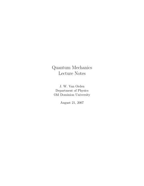
Figure 1.2: Electron diffraction pattern for a silver-gold alloy.<br />
1.4.2 Electron Diffraction<br />
In 1923 Louis Victor, Duc de Broglie was working in the physics laboratory of his<br />
older brother Maurice, Prince de Broglie. He had been giving considerable attention<br />
to Einstein’s light-quantum hypothesis. It occurred to him that if light which is<br />
classically a wave could behave as a particle, then classical particles could also behave<br />
as quantum waves. That is, he extended the wave-particle duality from light to<br />
particles. He proposed that the wavelength of a massive particle could be given by<br />
λ = h<br />
. (1.51)<br />
p<br />
This is now called the de Broglie wavelength.<br />
The implications of this for the Bohr model can be seen by considering the quantization<br />
condition (1.28). This can be rewritten as<br />
2πr = n h<br />
p<br />
= nλ . (1.52)<br />
That is, the circumference of the Bohr orbit is equal to an integral number of de<br />
Broglie wavelengths. de Broglie called these waves pilot waves.<br />
If particles can act as waves, it should be possible to see the diffraction and interference<br />
effects characteristic of waves with particles as well. Davisson and Germer<br />
demonstrated the diffraction of electrons from crystals in 1927. An example of an<br />
electron diffraction pattern for an silver-gold alloy is shown in Fig. 1.2. This phenomenon<br />
is now routinely used as an analytic tool in science and engineering.<br />
17
We are now left with the problem of how we can interpret a world where waves<br />
are particle and particles are waves. The resolution of this problem is associated with<br />
the development of quantum matrix mechanics by Heisenberg and of quantum wave<br />
mechanics of Schrödinger. Although the matrix mechanics appeared first in 1925<br />
with the wave mechanics appearing about half of a year later in 1926, we will begin<br />
our treatment of quantum dynamics by considering Schrödinger’s formulation of the<br />
theory.<br />
18
Chapter 2<br />
Mathematical Background to<br />
<strong>Quantum</strong> <strong>Mechanics</strong><br />
Before beginning our development of quantum mechanics, it is useful to first review<br />
linear algebra and analysis which forms the mathematical structure that we will use<br />
to describe the theory.<br />
2.1 Vector Spaces<br />
Consider a set of vectors for which the operations of vector addition and multiplication<br />
by a scalar are defined. The set forms a linear vector space if any operation of addition<br />
or scalar multiplication yields a vector in the original set. This means that the vector<br />
space is closed under these operations. It is also required that for arbitrary vectors<br />
A, B and C the operation of addition has the properties:<br />
and<br />
A + B = B + A (2.1)<br />
A + (B + C) = (A + B) + C . (2.2)<br />
There must also be a null vector 0 which acts as the identity under addition. That is<br />
Each vector A must also have an inverse −A such that<br />
The operation of scalar multiplication has the properties<br />
A + 0 = A . (2.3)<br />
A + (−A) = 0 . (2.4)<br />
α(A + B) = αA + αB (2.5)<br />
(α + β)A = αA + βA (2.6)<br />
α(βA) = (αβ)A , (2.7)<br />
19
where α and β are scalars. If the scalars are restricted to real numbers, then the<br />
the vector space is real. If the scalars are complex numbers, then the vector space is<br />
complex. For the moment we will restrict ourselves to real vector spaces. Clearly, the<br />
usual three-dimensional vectors that we use to describe particle motion satisfy these<br />
properties.<br />
A set of vectors {V1, V2, . . . , Vn} is said to be linearly independent if<br />
n�<br />
αiVi �= 0 (2.8)<br />
i=1<br />
except when all of the αi are zero. Any set linearly independent vectors form a basis<br />
and for an n-dimensional vector space the will be n vectors in any basis set. A basis<br />
set is said to span the vector space. The definition of implies that if we add some<br />
arbitrary vector V to the basis set we could now write<br />
or<br />
V −<br />
V =<br />
n�<br />
αiVi = 0 (2.9)<br />
i=1<br />
n�<br />
αiVi . (2.10)<br />
i=1<br />
This means that any vector in the vector space can be written as a linear combination<br />
of the basis vectors. This is the principle of linear superposition. The coefficients αi<br />
in the expansion are the components of the vector relative to the chosen basis set. For<br />
a three-dimensional vector space, any three non-coplanar vector will form a basis.<br />
One of the reasons for decomposing vectors into components relative to a set of<br />
basis vectors is that if<br />
n�<br />
A =<br />
(2.11)<br />
and<br />
then<br />
A + B =<br />
B =<br />
n�<br />
αiVi +<br />
i=1<br />
i=1<br />
αiVi<br />
n�<br />
βiVi , (2.12)<br />
i=1<br />
n�<br />
βiVi =<br />
i=1<br />
n�<br />
(αi + βi)Vi . (2.13)<br />
The addition of vectors then becomes equivalent to the addition of components.<br />
2.1.1 The Scalar Product<br />
An additional property that we associate with vectors is definition of a scalar or inner<br />
product which combines two vectors to give a scalar. A vector space on which a scalar<br />
20<br />
i=1
product is defined is called an inner product space. The scalar product which we are<br />
used to is defined as<br />
A · B = |A||B| cos γ , (2.14)<br />
where A and B are real vectors, |A| and |B| are the lengths of the two vectors, and<br />
γ is the angle between the vectors. This immediately implies that the inner product<br />
of a vector with itself is<br />
A · A = |A| 2<br />
(2.15)<br />
and that if A and B are perpendicular to one another (γ = 90 ◦ ) then<br />
The inner product is distributive. That is<br />
A · B = 0 . (2.16)<br />
A · (B + C) = A · B + A · C . (2.17)<br />
The definition of the inner product in terms of components relative to a set of basis<br />
vectors can be simplified by choosing a set of basis vectors which have unit length<br />
and are all mutually perpendicular. Such a basis is called an orthonormal basis. If<br />
we label the orthonoral basis vectors as ei for i = 1, . . . , n this means that<br />
If<br />
and<br />
Then<br />
ei · ej = δij for i, j = 1, . . . , n . (2.18)<br />
A =<br />
B =<br />
A · B =<br />
n�<br />
i=1<br />
αiei<br />
(2.19)<br />
n�<br />
βjej , (2.20)<br />
j=1<br />
n�<br />
αiβi . (2.21)<br />
This implies that we can now identify the components relative to an orthonormal<br />
basis as<br />
n�<br />
n�<br />
A · ei = A = αjej · ei = αjδij = αi . (2.22)<br />
j=1<br />
It should be noted that it is quite possible to deal with vector algebra in nonorthogonal<br />
bases, but the mathematics is much more complicated.<br />
21<br />
i=1<br />
j=1
2.1.2 Operators<br />
Now consider the possibility that there are operators that can act on a vector in the<br />
vector space and transform it into another vector in the space. That is<br />
Ωx = y , (2.23)<br />
where x and y are vectors in the space and Ω is some operator on the vectors in the<br />
space. An example of such an operator would be a rotation of a vector about some<br />
axis. If the operator has the properties<br />
and<br />
the operator is a linear operator.<br />
2.1.3 Matrix Notation<br />
Ω(cx) = c(Ωx) (2.24)<br />
Ω(x + y) = Ωx + Ωy (2.25)<br />
It is convenient to represent a vector in terms of a 1 × n column matrix which has the<br />
components of the vector relative to an orthonormal basis as elements. For example<br />
the three-dimensional vector x can be represented given by the column vector<br />
⎛ ⎞<br />
x = ⎝<br />
where xi = x · ei. The transpose of the matrix is<br />
x1<br />
x2<br />
x3<br />
x T = � x1 x2 x3<br />
⎠ , (2.26)<br />
� . (2.27)<br />
For two real vectors x and y, the inner product can then be written as<br />
x · y = x T y =<br />
If the vectors are complex, the inner product must be defined as<br />
x · y =<br />
3�<br />
i=1<br />
3�<br />
xiyi . (2.28)<br />
i=1<br />
x ∗ i yi<br />
(2.29)<br />
since the inner product of a vector with itself must give the length of the vector which<br />
is a real number. If we define the hermitian conjugate of a vector as<br />
x † = (x ∗ ) T , (2.30)<br />
22
then the inner product can be defined generally as<br />
x · y = x † y . (2.31)<br />
A linear operator acting on a vector produces another vector in the vector space.<br />
So, if we represent the vectors as column matrices, the operator acting on vector must<br />
also result in a column matrix. This means that an operator can be represented by<br />
an n × n matrix and the action of the operator on a vector is simply described as<br />
matrix multiplication. That is<br />
y = Ω x (2.32)<br />
where the components of Ω are Ωij and the components of y can be written as<br />
yi =<br />
n�<br />
j=1<br />
Ωijxj. (2.33)<br />
In order to simplify the notation for this kind of matrix transformation, it is convenient<br />
to use the Einstein summation convention. This convention assumes that any two<br />
repeated indices are to be summed over the appropriate range unless it is specifically<br />
stated otherwise. Using this convention we can write<br />
yi = Ωijxj , (2.34)<br />
where it is assumed that the repeated index j is summed from 1 to n.<br />
As an example the operator that produces a rotation of a three-dimensional vector<br />
through an angle φ about e3 is represented by the matrix<br />
⎛<br />
R (φ) = ⎝<br />
3<br />
cos φ − sin φ 0<br />
sin φ cos φ 0<br />
0 0 1<br />
⎞<br />
⎠ . (2.35)<br />
Since the operators are represented as matrices, they have the algebraic properties<br />
of matrices under multiplication. These properties are:<br />
1. Using the distributive property of matrix multiplication,<br />
A (x 1 + x 2) = A x 1 + A x 2 . (2.36)<br />
2. Since matrix multiplication is associative,<br />
� A B � x = A � B x � . (2.37)<br />
3. Multiplying a matrix by a constant is defined such that<br />
(cA)ij = cAij . (2.38)<br />
23
4. In general,<br />
or<br />
where<br />
defines the commutator of the matrices A and B.<br />
5. The identity matrix is the matrix with elements<br />
Then,<br />
6. If det(A) �= 0, then A has an inverse A −1 such that<br />
7. The transpose of a matrix is defined such that<br />
A B �= B A , (2.39)<br />
� A, B � �= 0 , (2.40)<br />
� A, B � ≡ A B − B A (2.41)<br />
(1)ij = δij . (2.42)<br />
1 A = A 1 = A . (2.43)<br />
A −1 A = A A −1 = 1 . (2.44)<br />
� A T �<br />
8. The complex conjugate of a matrix is defined such that<br />
� A ∗ �<br />
9. The hermitian conjugate of a matrix is defined such that<br />
So,<br />
10. A is hermitian if<br />
11. A is antihermitian if<br />
ij = Aji . (2.45)<br />
ij = (Aij) ∗ . (2.46)<br />
A † = � A ∗� T . (2.47)<br />
� A † �<br />
ij = (Aji) ∗ . (2.48)<br />
A † = A . (2.49)<br />
A † = −A . (2.50)<br />
24
12. A is unitary if<br />
Unitary transformations of the form<br />
have the hermitian conjugate<br />
So,<br />
A † = A −1 . (2.51)<br />
y = A x (2.52)<br />
y † = x † A † = x † A −1 . (2.53)<br />
y † y = x † A −1 A x = x † x . (2.54)<br />
This means that unitary transformations preserve the norm of a vector.<br />
2.1.4 The Eigenvalue Problem<br />
A problem of particular interest to us is the eigenvalue problem<br />
A x = λx (2.55)<br />
where λ is a constant. That is, we want to find all vectors x which when multiplied<br />
by A give the original vector times some constant λ. This can be rewritten as<br />
� A − λ1 � x = 0. (2.56)<br />
If A − λ1 has an inverse, then the only solution would be the trivial solution where<br />
x = 0. Therefore, this must not have an inverse which implies that<br />
det � A − λ1 � = 0 . (2.57)<br />
In three dimensions this will produce a cubic polynomial with three roots. So there<br />
will be three eigenvalues λi and three corresponding eigenvectors xi. In n dimensions<br />
this will be a polynomial of order n and there will be n eigenvalues with n<br />
corresponding eigenvectors.<br />
Consider the case where A is hermitian. The eigenvalue equation for the eigenvalue<br />
λi is<br />
A xi = λixi (2.58)<br />
where in this case the repeated index is not summed. If A is hermitian, the hermitian<br />
conjugate of the eigenvalue equation for the eigenvalue equation for eigenvalue λj is<br />
We can no multiply the first expression on the left by x †<br />
j<br />
by xi and then subtract the two expressions to give<br />
� �<br />
A − A xi = � λi − λ ∗ j<br />
x †<br />
j<br />
x †<br />
jA† = x †<br />
jA = λ∗jx †<br />
j . (2.59)<br />
25<br />
and the second on the right<br />
� x †<br />
j x i , (2.60)
or �<br />
λi − λ ∗� †<br />
j x jxi = 0 . (2.61)<br />
For the case where i = j, x †<br />
i x i > 0 if the eigenvector is to be nontrivial. This then<br />
requires that<br />
λi − λ ∗ i = 0 . (2.62)<br />
Therefore, the λi must be real for all i. Now, for i �= j, if the eigenvalues are not<br />
degenerate this requires that<br />
x †<br />
j x i = 0 . (2.63)<br />
So the eigenvectors are orthogonal. In the case where two or more eigenvalues have<br />
the same value which means that they are degenerate, the eigenvectors associated<br />
with these eigenvalues will be orthogonal to all of the remaining eigenvectors, but<br />
may not be mutually orthogonal. In this case it is necessary to construct linear<br />
combinations of the eigenvectors that are mutually orthogonal. Now multiply (2.58)<br />
by some arbitrary constant c. This gives<br />
or<br />
cA x i = cλix i , (2.64)<br />
A (cx i) = λi(cx i) . (2.65)<br />
This means that the normalization of the eigenvectors are not determined by the<br />
eigenvalue equation. As a result we can always choose the the eigenvectors to be of<br />
unit length. We have now shown that for a hermitian matrix we will always obtain<br />
real eigenvalues and the eigenvectors can be normalized to for an orthonormal set of<br />
basis vectors.<br />
Now consider the case where a set of vectors xi are eigenvector for two different<br />
operators Λ and Ω such that<br />
(2.66)<br />
and<br />
Λ x i = λix i<br />
Using the eigenvalue equation we can write<br />
Ω x i = ωix i . (2.67)<br />
Λ Ω x i = Λωix i = ωiΛ x i = ωiλix i = Ω(λix i) = Ω Λ x i , (2.68)<br />
where it has been assumed that the operators are linear in the second and fourth<br />
steps. This implies that<br />
(Λ Ω − Ω Λ)x i = [Λ, Ω]x i = 0 . (2.69)<br />
Since this must be true for all of the eigenvectors in the set, it follows that<br />
[Λ, Ω] = 0 . (2.70)<br />
26
That is, operators with common eigenvectors commute.<br />
Next, let the vectors x i represent a normalized set of eigenvectors of the operator<br />
A such that<br />
A xi = λix i . (2.71)<br />
We can now define the outer product of these eigenvectors as<br />
Ξ = x<br />
i ix †<br />
i . (2.72)<br />
By the rules of matrix multiplication, the Ξ i must be an n × n matrix. Now, define<br />
Ξ =<br />
n�<br />
Ξ =<br />
i<br />
i=1<br />
n�<br />
i=1<br />
xix †<br />
i . (2.73)<br />
Consider the case where this operates on an arbitrary eigenvector in this set. That is<br />
Therefore,<br />
Ξ x j =<br />
n�<br />
i=1<br />
Ξ i x j =<br />
n�<br />
i=1<br />
n�<br />
i=1<br />
x ix †<br />
i x j =<br />
x ix †<br />
i<br />
n�<br />
i=1<br />
x iδij = x j . (2.74)<br />
= 1 . (2.75)<br />
This is called the completeness relation for the set of eigenvectors.<br />
Again, consider an operator A which has eigenvectors x i with eigenvalues λi. That<br />
is,<br />
A x i = λix i . (2.76)<br />
With the solution of the eigenvalue problem, we now have two bases that have been<br />
defined, the original basis set given by the vectors ei and the basis set composed of<br />
the normalized eigenvectors xi. That is the eigenvectors are defined in terms of the<br />
original basis vectors as<br />
x i =<br />
n�<br />
j=1<br />
e je †<br />
j x i<br />
and the components of the operator matrix are given by<br />
(2.77)<br />
(A)ij = e †<br />
i A e j . (2.78)<br />
We can also expand the original basis vectors in terms of the eigenvectors by using<br />
the completeness of the eigenvectors to give<br />
e i = 1 e i =<br />
27<br />
n�<br />
j=1<br />
x jx †<br />
j e i . (2.79)
Similarly, we can now define a new matrix operator � A which is defined in the basis<br />
of eigenvectors and has components given by<br />
�A kl = x †<br />
k A x l = x †<br />
k λlx l = λlx †<br />
k x l = λlδkl . (2.80)<br />
This means that the operator represented in the basis of eigenvectors is diagonal.<br />
These components can be rewritten in terms of the original matrix representation of<br />
the operator by using the completeness of the basis vectors e i as<br />
( � A)kl = x †<br />
k<br />
=<br />
=<br />
n�<br />
i=1<br />
n�<br />
i=1<br />
n�<br />
i=1<br />
n�<br />
j=1<br />
n�<br />
j=1<br />
e ie †<br />
i A<br />
n�<br />
j=1<br />
e je †<br />
j x l<br />
x †<br />
k e ie †<br />
i A e je †<br />
j x l<br />
Now, define the matrix U with components given by<br />
and note that<br />
Then,<br />
or<br />
x †<br />
k e i =<br />
n�<br />
(xk) ∗ m(ei)m =<br />
m=1<br />
(U)jl = e †<br />
j x l = (x l)j<br />
n�<br />
((ei) ∗ m(xk)m) ∗ =<br />
m=1<br />
( � A)kl =<br />
n�<br />
i=1<br />
x †<br />
k e i(A)ije †<br />
j x l . (2.81)<br />
(2.82)<br />
�<br />
e †<br />
ix �∗ k = (U) ∗ ik = (U † )ki . (2.83)<br />
n�<br />
(U † )ki(A)ij(U)jl<br />
j=1<br />
(2.84)<br />
�A = U † A U . (2.85)<br />
This transformation then converts from one representation of the operator to the<br />
other. From the definition of U we can write that<br />
or<br />
This shows that<br />
n�<br />
(U † )ik(U)kj =<br />
k=1<br />
n�<br />
k=1<br />
x †<br />
i e ke †<br />
k x j = x †<br />
i x j = δij<br />
(2.86)<br />
U † U = 1 . (2.87)<br />
U † = U −1 , (2.88)<br />
28
so this matrix is unitary and the transformation<br />
�A = U −1 A U (2.89)<br />
is called a unitary transformation. This means that the operator A is diagonalized<br />
by a unitary transformation. This transformation can be inverted to give<br />
A = U � A U −1 . (2.90)<br />
Eventually we will need to define functions of operators. In this case, the function<br />
is always defined as a power series<br />
f(A) =<br />
∞�<br />
cnA n<br />
n=0<br />
(2.91)<br />
where the expansion coefficients are the same as the Taylor series for the same function<br />
of a scalar. That is<br />
∞�<br />
f(z) = cnz n . (2.92)<br />
n=0<br />
Unless the matrix A has special algebraic properties, the evaluation of the function<br />
as an infinite series can be very difficult. This can be simplified by using the unitary<br />
transformation that diagonalizes the operator. To see how this works consider the<br />
third power of the operator. Using the unitary of the transformation matrix we can<br />
write<br />
A 3 = A A A = U U −1 A U U −1 A U U −1 A U U −1 = U Ã � A � A U −1 = U � A 3<br />
U −1 . (2.93)<br />
This helpful because any power of a diagonal matrix is given by simply raising the<br />
diagonal elements to the same power. That is,<br />
( � A n<br />
)ij = λ n i δij . (2.94)<br />
It is easy to see how this method can be extended to any power of the operator. Then,<br />
f(A) =<br />
∞�<br />
n=0<br />
cnU � A n<br />
U −1 �<br />
∞�<br />
= U<br />
n=0<br />
cn � A n<br />
�<br />
U −1 = Uf( � A) U −1 , (2.95)<br />
where �<br />
f( � �<br />
A) = f(λi)δij . (2.96)<br />
ij<br />
29
Example: Find the eigenvalues and eigenvectors for the matrix<br />
⎛<br />
0 1<br />
⎞<br />
0<br />
A = ⎝ 1 0 1 ⎠ . (2.97)<br />
0 1 0<br />
The eigenvalues are obtained by requiring that<br />
Or<br />
So<br />
⎛<br />
0 = det ⎝<br />
−λ 1 0<br />
1 −λ 1<br />
0 1 −λ<br />
Now the eigenvectors must satisfy the equation<br />
⎛<br />
−λ 1 0<br />
⎞ ⎛<br />
1<br />
⎝ 1 −λ 1 ⎠ ⎝ a<br />
0 1 −λ b<br />
⎞<br />
det � A − λ1 � = 0 . (2.98)<br />
⎠ = −λ � λ 2 − 1 � − 1 (−λ) = −λ � λ 2 − 2 �<br />
(2.99)<br />
λ = 0, ± √ 2 . (2.100)<br />
⎞<br />
⎠ = 0 . (2.101)<br />
Only two of the linear equations produced by this matrix expression can be<br />
independent since the matrix is required to have a determinant of zero. The<br />
eigenvalue problem determines the eigenvectors only up to a multiplicative constant.<br />
For this reason, the top component of the column vector has been arbitrarily<br />
chosen to be 1. We will choose the normalization of the eigenvectors<br />
such that they are unit vectors. This leads to three linear equations<br />
The first of these can be solved to give<br />
The second can be solved to give<br />
So for λ = √ 2,<br />
−λ + a = 0 (2.102)<br />
1 − λa + b = 0 (2.103)<br />
a − λb = 0 . (2.104)<br />
a = λ . (2.105)<br />
b = λa − 1 = λ 2 − 1 . (2.106)<br />
⎛<br />
x1 = N1 ⎝<br />
30<br />
1<br />
√ 2<br />
1<br />
⎞<br />
⎠ . (2.107)
The normalization constant is chosen such that x †<br />
i x i = 1. So<br />
1 = N 2 i<br />
Solving this for Ni gives<br />
�<br />
1 ∗ a<br />
⎛<br />
�<br />
∗ b ⎝<br />
Therefore, for this eigenvector<br />
For λ = 0,<br />
where<br />
For λ = − √ 2,<br />
where<br />
Ni =<br />
N1 =<br />
N2 =<br />
1<br />
a<br />
b<br />
⎞<br />
⎠ = N 2 i (1 + |a| 2 + |b| 2 ) . (2.108)<br />
1<br />
� . (2.109)<br />
1 + |a| 2 + |b| 2<br />
1<br />
√ =<br />
1 + 2 + 1 1<br />
. (2.110)<br />
2<br />
⎛<br />
x2 = N2 ⎝<br />
1<br />
0<br />
−1<br />
⎞<br />
⎠ , (2.111)<br />
1<br />
√ =<br />
1 + 0 + 1 1<br />
√ . (2.112)<br />
2<br />
⎛<br />
x3 = N2 ⎝<br />
N3 =<br />
1<br />
− √ 2<br />
1<br />
⎞<br />
⎠ , (2.113)<br />
1<br />
√ =<br />
1 + 2 + 1 1<br />
. (2.114)<br />
2<br />
Note that for these eigenvectors x †<br />
i x j = δij. So the eigenvectors for a set of<br />
orthonormal basis vectors.<br />
2.2 The Continuum Limit<br />
Consider a system of n equal masses connected by equivalent springs between the<br />
masses and connecting the end masses to fixed walls. The system is allowed to move<br />
in one dimension. The case of n = 5 is shown in Fig. 2.1. The equilibrium position<br />
of mass i is given by xi. The equations of motion of the masses can be written in<br />
31
Figure 2.1: Five equal masses coupled by identical springs. The top part of the figure<br />
shows the equilibrium position while the bottom part shows the system with displaced<br />
masses. The equilibrium positions are given by xi and the displacement of each mass<br />
from equilibrium is given by φi.<br />
terms of the displacement of the masses φi from their equilibrium positions by<br />
m ¨ φ1(t) = k (φ2(t) − φ1(t)) − kφ1(t)<br />
m ¨ φ2(t) = k (φ3(t) − φ2(t)) − k (φ2(t) − φ1(t))<br />
m ¨ φ3(t) = k (φ4(t) − φ3(t)) − k (φ3(t) − φ2(t))<br />
.<br />
m ¨ φn−1(t) = k (φn(t) − φn−1(t)) − k (φn−1(t) − φn−2(t))<br />
m ¨ φn(t) = −kφn(t) − k (φn(t) − φn−1(t)) (2.115)<br />
This set of coupled second-order differential equation can be written in matrix form<br />
as<br />
⎛<br />
⎜<br />
⎝<br />
¨φ1(t)<br />
¨φ2(t)<br />
¨φ3(t)<br />
¨φ4(t)<br />
.<br />
¨φn−1(t)<br />
¨φn(t)<br />
⎞<br />
⎟<br />
⎠<br />
= k<br />
m<br />
⎛<br />
⎜<br />
⎝<br />
−2 1 0 0 · · · 0 0 0<br />
1 −2 1 0 · · · 0 0 0<br />
0 1 −2 1 · · · 0 0 0<br />
0 0 1 −2 · · ·<br />
. ..<br />
0 0 0<br />
.<br />
.<br />
.<br />
.<br />
0 0 0 0 · · · 1 −2 1<br />
0 0 0 0 · · · 0 1 −2<br />
.<br />
.<br />
.<br />
⎞ ⎛<br />
⎟ ⎜<br />
⎟ ⎜<br />
⎟ ⎜<br />
⎟ ⎜<br />
⎟ ⎜<br />
⎟ ⎜<br />
⎟ ⎜<br />
⎟ ⎜<br />
⎟ ⎜<br />
⎠ ⎝<br />
φ1(t)<br />
φ2(t)<br />
φ3(t)<br />
φ4(t)<br />
.<br />
φn−1(t)<br />
φn(t)<br />
(2.116)<br />
Since we would expect that the masses will oscillate when set in motion, it is logical<br />
to look for solutions of the form<br />
⎞<br />
⎟ .<br />
⎟<br />
⎠<br />
φi(t) = ηie iωt . (2.117)<br />
32
Substituting this into the matrix form of the equations of motion gives<br />
⎛<br />
⎞ ⎛ ⎞<br />
2 −1 0 0 · · · 0 0 0 η1<br />
⎜ −1 2 −1 0 · · · 0 0 0 ⎟ ⎜<br />
⎟ ⎜ η2<br />
⎟<br />
⎜<br />
k<br />
⎜ 0 −1 2 −1 · · · 0 0 0 ⎟ ⎜<br />
⎟ ⎜ η3<br />
⎟<br />
⎜ 0 0 −1 −2 · · · 0 0 0 ⎟ ⎜<br />
⎟ ⎜ η4<br />
⎟ = ω<br />
m ⎜<br />
.<br />
⎜<br />
. . . . ..<br />
⎟ ⎜ ⎟<br />
. . . ⎟ ⎜<br />
⎟ ⎜<br />
. ⎟<br />
⎝ 0 0 0 0 · · · −1 2 −1 ⎠ ⎝ ηn−1 ⎠<br />
0 0 0 0 · · · 0 −1 2<br />
2<br />
⎛<br />
η1<br />
⎜ η2<br />
⎜ η3<br />
⎜ η4<br />
⎜<br />
.<br />
⎝ ηn−1<br />
ηn<br />
ηn<br />
⎞<br />
⎟ . (2.118)<br />
⎟<br />
⎠<br />
This is now an eigenvalue problem with n eigenvalues ω 2 i and corresponding n eigenvectors<br />
η i . This is an example of a common problem in classical mechanics involving<br />
small oscillations of coupled oscillators. The eigenvectors are called the normal modes<br />
of the system and the corresponding frequencies are the normal mode frequencies.<br />
This can be solved for any value of n.<br />
It is interesting to consider the case where n → ∞ with the total mass fixed. We<br />
can do this be examining one of the equations of motion<br />
m ¨ φi(t) = k (φi+1(t) − φi(t)) − k (φi(t) − φi−1(t)) . (2.119)<br />
It is convenient at this point to change the way that we label the masses. Instead of<br />
using the subscript i, we can label each mass by its equilibrium position xi = i∆x<br />
where<br />
∆x = L<br />
, (2.120)<br />
n + 1<br />
with L being the separation between the anchoring walls. The differential equation<br />
can then be rewritten as<br />
m ∂2<br />
∂t2 φ(xi, t) = k (φ(xi+1, t) − φ(xi, t)) − k (φ(xi, t) − φ(xi−1, t)) . (2.121)<br />
If the total mass of the system is M then the mass of each particle is<br />
m = M<br />
. (2.122)<br />
n<br />
We can now rewrite the differential equation as<br />
m ∂2<br />
∂t2 φ(xi, t) = k (φ(xi + ∆x, t) − φ(xi, t)) − k (φ(xi−1 + ∆x, t) − φ(xi−1, t)) .<br />
(2.123)<br />
Since as n becomes large ∆x will be come small for fixed L, we can expand the<br />
displacement functions to first order in ∆x to give<br />
m ∂2<br />
∂t2 φ(xi, t) = k ∂φ<br />
∂x (xi, t)∆x − k ∂φ<br />
∂x (xi−1, t)∆x<br />
�<br />
∂φ<br />
= k∆x<br />
∂x (xi, t) − ∂φ<br />
∂x (xi<br />
�<br />
− ∆x, t)<br />
= k(∆x) 2 ∂2 φ<br />
∂x 2 (xi, t) . (2.124)<br />
33
Note that<br />
m = M M L M n + 1<br />
= =<br />
n L n L n ∆x ∼ = M<br />
∆x<br />
L<br />
(2.125)<br />
for large n. If we define the linear mass density as<br />
and Young’s Modulus as<br />
we obtain the wave equation<br />
µ = M<br />
L<br />
∂2 1<br />
φ(x, t) −<br />
∂x2 v2 (2.126)<br />
Y = k∆x , (2.127)<br />
∂2 φ(x, t) = 0 , (2.128)<br />
∂t2 where<br />
v 2 = Y<br />
. (2.129)<br />
M<br />
This is a second-order partial differential equation in x and t. Since the ends of the<br />
system are fixed, the amplitude function must satisfy the spatial boundary conditions<br />
φ(0, t) = φ(L, t) = 0 . (2.130)<br />
Any particular solution must also involve the imposition of initial conditions for φ<br />
and ∂φ<br />
∂t .<br />
Recall that for any finite n, there will be n eigenvalues (eigenfrequencies) and<br />
eigenvectors. Since the wave equation is the result of the limiting behavior of the<br />
system when the n → ∞, we should expect that we should be able to express the<br />
solution of the wave equation in terms of an eigenvalue problem with an infinite<br />
number of eigenfrequencies and eigenvectors. The standard method for obtaining<br />
such a solution involves the procedure of separation of variables. To do this we<br />
assume that the amplitude function can be factored such that<br />
Substituting this into (2.128) and rearranging gives<br />
1<br />
X(x)<br />
φ(x, t) = X(x)T (t) . (2.131)<br />
∂2X(x) 1<br />
−<br />
∂x2 v2T (t)<br />
∂2T (t)<br />
= 0 . (2.132)<br />
∂t2 Since each of the two terms depends only on a single variable, the only way this can<br />
be satisfied for all values of x and t is for each of the two terms to be constant, with<br />
the constants adding to 0. If we choose the constant such that<br />
1 ∂<br />
X(x)<br />
2X(x) ∂x2 = −k2 , (2.133)<br />
34
then we obtain the differential equation<br />
or<br />
∂ 2 X(x)<br />
∂x 2 = −k2 X(x) , (2.134)<br />
∂ 2 X(x)<br />
∂x 2 + k2 X(x) = 0 . (2.135)<br />
This is the familiar harmonic equation which has solutions of the form<br />
X(x) = c1 cos(kx) + c2 sin(kx) . (2.136)<br />
The first of the spatial boundary conditions requires that X(0) = 0 which requires<br />
that c1 = 0. The second boundary condition requires that X(L) = c2 sin(kL) = 0.<br />
This can only be satisfied if<br />
kL = nπ , (2.137)<br />
where n > 0. Then for each value of n we have<br />
kn = πn<br />
L<br />
(2.138)<br />
Note that (2.134) is of a form similar to a matrix eigenequation, where the matrix<br />
is replaced by the differential operator ∂2<br />
∂x2 and the eigenvalue is given by −k2 eigenvectors are replaced by the functions<br />
. The<br />
�<br />
nπx<br />
�<br />
Xn(x) = Nn sin .<br />
L<br />
(2.139)<br />
Since there are an infinite number of values for n, there are an infinite number of<br />
eigenvalues and eigenvectors or eigenfunctions.<br />
The differential operator is linear differential operator since<br />
where a is a complex constant, and<br />
∂2 ∂2<br />
af(x) = a f(x) , (2.140)<br />
∂x2 ∂x2 ∂2 ∂x2 (f(x) + g(x)) = ∂2f(x) ∂x2 + ∂2g(x) ∂x2 . (2.141)<br />
This means that we can expand any nonsingular function defined on the interval<br />
0 ≤ x ≤ L as a linear combination of the eigenfunctions. That is<br />
f(x) =<br />
where the an are complex constants.<br />
∞�<br />
anXn(x) , (2.142)<br />
n=1<br />
35
We can now define an inner product as<br />
The inner product of any two eigenfunctions is then<br />
0<br />
� L<br />
f · g = dxf ∗ (x)g(x) . (2.143)<br />
0<br />
0<br />
� L<br />
dxX ∗ � L �<br />
mπx<br />
� �<br />
nπx<br />
�<br />
m(x)Xn(x) = NmNn dx sin sin = N<br />
2L 2L<br />
2 L<br />
n<br />
2 δmn . (2.144)<br />
This means that the eigenfunctions are orthogonal and can be normalized by choosing<br />
�<br />
2<br />
Nn = . (2.145)<br />
L<br />
The completeness relation for the normalized eigenfunctions is<br />
∞�<br />
Xn(x)X ∗ n(x ′ ) = δ(x − x ′ ) , (2.146)<br />
n=1<br />
where δ(x − x ′ ) is the Dirac delta function and is defined such that:<br />
1. δ(x − a) = 0 for all x �= a.<br />
2. � � x1<br />
1 if x0 < a < x1<br />
dxδ(x − a) =<br />
0 if a < x0 or a > x1<br />
x0<br />
3. � � x1<br />
f(a) if x0 < a < x1<br />
dxf(x)δ(x − a) =<br />
0 if a < x0 or a > x1<br />
x0<br />
4. � x1<br />
dxf(x)δ ′ �<br />
′ −f (a) if x0 < a < x1<br />
(x − a) =<br />
0 if a < x0 or a > x1<br />
5.<br />
x0<br />
δ(f(x)) = �<br />
i<br />
(2.147)<br />
(2.148)<br />
(2.149)<br />
1<br />
�<br />
� df<br />
� δ(x − xi) (2.150)<br />
�<br />
dx x=xi<br />
where the xi are all of the simple zeros of f(x). A common particular case of<br />
this identity is<br />
δ(cx) = 1<br />
δ(x) , (2.151)<br />
|c|<br />
where c is a constant.<br />
36
This kind of infinite-dimensional inner-product vector space with the eigenvectors<br />
composed of continuous functions defined on some interval is called a Hilbert space.<br />
If we now substitute (2.133) into (2.132) and rearrange the result, we obtain<br />
∂ 2 T (t)<br />
∂t 2 + v2 k 2 T (t) = 0 . (2.152)<br />
Again this is the harmonic equation. Since we have already fixed the eigenvalue using<br />
the spatial equation, if we define<br />
the solution to this differential equation is of the form<br />
ωn = vkn , (2.153)<br />
Tn(t) = An cos(ωnt) + Bn sin(ωnt) . (2.154)<br />
The complete wave function for a given n is then<br />
�<br />
2<br />
φn(x, t) = Xn(t)Tn(t) =<br />
L sin(knx) (An cos(ωnt) + Bn sin(ωnt)) (2.155)<br />
and a general solution for the wave function is<br />
∞�<br />
∞�<br />
�<br />
2<br />
φ(x, t) = φn(x, t) =<br />
L sin(knx) (An cos(ωnt) + Bn sin(ωnt)) . (2.156)<br />
n=1<br />
n=1<br />
The constants An and Bn are determined by imposing the initial conditions in time,<br />
φ(x, 0) = f(x) (2.157)<br />
and<br />
�<br />
∂φ(x, t) �<br />
�<br />
∂t � = g(x) . (2.158)<br />
t=0<br />
We have now outlined the mathematical foundations that we will use to describe<br />
quantum mechanics. The mathematical solution of most quantum mechanical problems<br />
begins with the time-dependent Schrödinger equation which is a partial differential<br />
equation that is second order in the spatial variables and first order in time.<br />
A particular solution to this equation requires imposing appropriate boundary conditions<br />
in space and time. The basic procedure for solution follows that presented<br />
above and can be summarized as:<br />
1. A separable solution in space and time is assumed.<br />
2. Substituting this solution in the Schrödinger equation and separating variables<br />
results in an eigenvalue equation in the spatial variables called the timeindependent<br />
Schrödinger equation.<br />
37
3. Imposing the spatial boundary conditions determines the eigenvalues and eigenfunctions.<br />
4. We will show that the differential operator in the spatial equation is hermitian.<br />
This implies that the eigenvalues will be real and the eigenfunctions are<br />
orthonormal.<br />
5. The differential equation in time can be solved for each eigenvalue.<br />
6. The complete wave function for each eigenvalue can then be constructed.<br />
7. The general solution of the time-dependent Schrödinger equation can be constructed<br />
as a linear combination of these solutions where the coefficients in the<br />
expansion are determined by the initial condition in time.<br />
We will now examine the physical origins and interpretation of the Schrödinger<br />
equation.<br />
38
Chapter 3<br />
The Schrödinger Equation<br />
3.1 Wave Particle Duality<br />
Now we are left with the problem of having to make sense out the reality that waves<br />
can also behave like particles and particles can behave like waves. To motivate how<br />
we are going to find a formulation of quantum mechanics that allows this to happen,<br />
it is useful to consider the classical situation. In particular consider the case of light<br />
waves and the two-slit diffraction problem.<br />
Assume that we have a plane wave illuminating the slits from the left. When the<br />
waves strike the screen with the slits, we can describe the part of the wave which passes<br />
through the slits using Huygen’s principle. As the wave front strikes the slit, each<br />
point in the slit radiates a spherical wave and the electromagnetic wave emanating<br />
from the slit is the total of the spherical waves from all of the points. The wave from<br />
the upper slit can be represented by the electric field E1(r, t) and that from the lower<br />
slit as E2(r, t). The intensity of the wave is proportional to the absolute square of<br />
the electric field. If the bottom slit is covered and light can pass only through the<br />
upper slit we see an image of the slit which is proportional to |E1(r, t)| 2 on the second<br />
screen and similarly covering the upper slit while light passes through the lower slit<br />
gives an image of slit two proportional to |E2(r, t)| 2 . This situation is illustrated in<br />
Fig. 3.1 where the intensity of the light along the second screen is illustrated by the<br />
curve to the right of the screen.<br />
Now in the case when both slits are open, the total field is given by the sum of<br />
the fields due to each slit E(r, t) = E1(r, t) + E2(r, t) since Maxwell’s equations are<br />
linear. The intensity at the screen will then be proportional to<br />
|E1(r, t) + E2(r, t)| 2 = |E1(r, t)| 2 + |E2(r, t)| 2 + 2E1(r, t) · E2(r, t) . (3.1)<br />
The result is illustrated by Fig. 3.2. The interference pattern is due to the cross term<br />
(the interference term).<br />
Now consider the situation where the the two slits are now being illuminated by<br />
a beam of electrons which is larger than the distance between the slits and where the<br />
39
Figure 3.1: Images of the slits is illuminated individually<br />
Figure 3.2:<br />
40
directions of the velocities of the electrons vary by a small amount. If the electrons<br />
behaved only like particles the result would appear as in the case of Fig. 3.1 with<br />
the total count of electrons hitting the screen represented by the sum of the two<br />
curves on the right. However, since we know from our previous discussions that the<br />
electrons have wave-like properties, the result is an interference pattern as illustrated<br />
in Fig. 3.2. Furthermore, the interference pattern is made up of a large number of<br />
individual electrons striking the screen so that the electrons can indeed still be seen<br />
as particles. One way of looking at this phenomenon is to introduce de Broglie’s<br />
pilot waves. These waves determine in some fashion where the electrons will go. This<br />
means that we would replace the electric field from slit one in our classical example<br />
by a wave function Ψ1(r, t) and that from slit 2 by Ψ2(r, t). In order for us to get<br />
the interference pattern, these two wave functions must add to give the total wave<br />
function. This requires that the wave equation, of which these wave functions Ψ1 and<br />
Ψ2 are solutions, must be a linear differential equation. The number of electrons that<br />
strike the second screen at a given time must then be represented by the absolute<br />
square of the total wave function. That is, |Ψ1(r, t) + Ψ2(r, t)| 2 .<br />
It is reasonable to ask the question: “Which slit does each electron pass through?”<br />
Imagine that we place a laser beam on the right side of the screen containing the two<br />
slits with the beam parallel to this screen. We can then detect whether an electron<br />
passes through slit 1 or slit 2 by looking for a flash of light due to Compton scattering<br />
of a photon in the laser beam from each electron as it passes through a slit. Now we<br />
perform the experiment again and record not only the position of the electron as it<br />
strikes the second screen, but also which slit it passes through. All of the events can<br />
then be classified by which slit the electron passed through. If we now assemble all of<br />
these events together we will see that the distribution is given by |Ψ1| 2 + |Ψ2| 2 . The<br />
interference pattern has disappeared and we get the result that we would get if the<br />
electrons only behaved as particles.<br />
The source of this problem is that in order to measure the positions of the electrons<br />
to determine through which slit they passed, we have scattered photon’s from the<br />
electrons. This scattering affects the motion of the electrons and eliminates the<br />
interference pattern. One way we can imagine that we could reduce this effect is to<br />
decrease the intensity of the laser beam. This means that there are fewer photons<br />
to scatter from the electrons so we will decrease the chance that such a scattering<br />
takes place. The result is that we will now see events where the electrons strike the<br />
second screen but for which we see no flash indicating which hole they went through.<br />
We will now have three classes of events: those which are seen to pass through slit 1,<br />
those that are seen to pass through slit 2 and those where we do not know through<br />
which slit they passed. If we look at electrons in the first two categories we again see<br />
no interference, but those in the third category where there is no information about<br />
which slot they passed through will show an interference pattern. So we have done<br />
nothing to resolve our problem.<br />
The problem might be that we have chosen the wrong approach. After all, we<br />
41
know from Einstein that the photons will each have energy E = hν so those photons<br />
that scatter will still change the motion of the electrons in the same way regardless<br />
of the intensity of the beam. For this reason we can consider another approach. We<br />
will keep the high intensity but decrease the frequency (increase the wavelength). If<br />
we now redo the experiment under these conditions, we will still see that for electrons<br />
that are measured to go through either of the slits we will have no interference pattern.<br />
However, as the wavelength increases as we reduce the energy of the photons, we will<br />
reach the point that the wavelength becomes greater than the separation between<br />
the two slits and we will no longer be able to resolve the positions of the electrons to<br />
determine which slit they passed through. We will then start to see the interference<br />
pattern again. This shows that there is no way that we can determine the path of the<br />
electron without affecting the motion of the electrons. Although we have framed this<br />
discussion in terms of photons scattering from electrons, any means of determining<br />
the slit through which an electron passes will have the same problems.<br />
We then have a fundamental limitation on our ability to determine the trajectories<br />
of a given electron. We can no longer follow the trajectory of the electron through<br />
the system to the point where it strikes the second screen without changing that<br />
motion. One of the basic requirements that Heisenberg used in constructing his<br />
matrix mechanics was that only the aspects of the theory that described observable<br />
quantities are essential to the theory. Since we have now demonstrated that we<br />
cannot measure the trajectories of the electrons, the concept that quantum particles<br />
must follow definite trajectories, as in classical mechanics, need not be contained in<br />
quantum mechanical theories.<br />
3.2 Wave Packets<br />
To get a better understanding of how this comes about, lets return to the basic problem<br />
of the motion of classical waves. If we want to try to localize the energy carried<br />
by such a wave, we need to construct a wave packet. This is done by representing the<br />
wave function as a linear superposition of plane waves. In one dimension this can be<br />
written as<br />
� ∞<br />
Ψ(x, t) = dkφ(k)e i(kx−ωt) , (3.2)<br />
−∞<br />
where ω is some function of k. At t = 0 this gives<br />
� ∞<br />
Ψ(x, 0) = dkφ(k)e ikx<br />
so the initial wave packet is just the Fourier transform of φ(k).<br />
For the purposes of our discussion, consider the case where φ(k) is a gaussian<br />
−∞<br />
1<br />
−<br />
φ(k) = e 2 α2 (k−k0) 2<br />
42<br />
(3.3)<br />
(3.4)
where α and k0 are constants. The wave packet at t = 0 is then given by<br />
� ∞<br />
Ψ(x, 0) =<br />
−∞<br />
1<br />
−<br />
dke 2 α2 (k−k0) 2<br />
e ikx . (3.5)<br />
We can now change the integration variable to q = k − k0 so that<br />
� ∞<br />
� ∞<br />
Ψ(x, 0) =<br />
−∞<br />
1<br />
−<br />
dqe 2 α2q2 e i(q+k0)x ik0x<br />
= e<br />
−∞<br />
1<br />
−<br />
dqe 2 α2q2 +ixq<br />
. (3.6)<br />
This integral can be found in any good set of integral tables. The result is then<br />
Ψ(x, 0) =<br />
The intensity of the wave will be related to<br />
√ 2π<br />
α eik0x e − x2<br />
2α 2 . (3.7)<br />
|Ψ(x, 0)| 2 = 2π x2<br />
e− α<br />
α2 2 (3.8)<br />
which is a gaussian.<br />
Now we can define the average value of some power of x over this distribution as<br />
〈x n � ∞<br />
−∞<br />
〉 =<br />
dxxn |Ψ(x, 0)| 2<br />
. (3.9)<br />
dx|Ψ(x, 0)|2<br />
For the special case we are considering<br />
� ∞<br />
−∞<br />
� ∞<br />
−∞<br />
� ∞<br />
−∞<br />
dx|Ψ(x, 0)| 2 = 2π<br />
α2 � ∞<br />
x2<br />
−<br />
dxe α<br />
−∞<br />
2 =<br />
since the integrand is odd and<br />
� ∞<br />
dxx 2 |Ψ(x, 0)| 2 = 2π<br />
α2 � ∞<br />
−∞<br />
Using these expressions yields<br />
and<br />
2π 3<br />
2<br />
α<br />
, (3.10)<br />
dxx|Ψ(x, 0)| 2 = 2π<br />
α2 � ∞<br />
x2<br />
−<br />
dxxe α<br />
−∞<br />
2 = 0 , (3.11)<br />
� x 2 � =<br />
−∞<br />
dxx 2 x2<br />
−<br />
e α2 = π 3<br />
2 α . (3.12)<br />
〈x〉 = 0 (3.13)<br />
π 3<br />
2 α<br />
2π 3 2<br />
α<br />
= α2<br />
2<br />
. (3.14)<br />
If we now define the root mean square deviation as<br />
∆x ≡ � 〈|x − 〈x〉 | 2 �<br />
〉 = 〈x2 〉 − 〈x〉 2 , (3.15)<br />
43
for the special case we are considering here we get<br />
�<br />
α2 ∆x =<br />
2 − 02 = α √ . (3.16)<br />
2<br />
We can now do something similar for the wave number k by defining<br />
〈k n � ∞<br />
−∞<br />
〉 =<br />
dkkn |φ(k)| 2<br />
� ∞<br />
−∞ dk|φ(k)|2<br />
. (3.17)<br />
For the special case being considered here<br />
� ∞<br />
dk|φ(k)| 2 � ∞<br />
= dke −α2 (k−k0) 2<br />
� ∞<br />
= dqe −α2q2 √<br />
π<br />
= ,<br />
α<br />
(3.18)<br />
−∞<br />
� ∞<br />
dkk|φ(k)| 2 =<br />
−∞<br />
and<br />
� ∞<br />
dkk<br />
−∞<br />
2 |φ(k)| 2 =<br />
So,<br />
and<br />
=<br />
=<br />
=<br />
−∞<br />
−∞<br />
� ∞<br />
dkke<br />
−∞<br />
−α2 (k−k0) 2<br />
� ∞<br />
= dq(q + k0)e<br />
−∞<br />
−α2q2 � ∞<br />
dqqe −α2q2 � ∞<br />
+ k0 dqe −α2q2 √<br />
π<br />
= k0<br />
α<br />
−∞<br />
−∞<br />
(3.19)<br />
� ∞<br />
dkk<br />
−∞<br />
2 e −α2 (k−k0) 2<br />
� ∞<br />
= dq(q + k0)<br />
−∞<br />
2 e −α2q2 � ∞<br />
dqq<br />
−∞<br />
2 e −α2q2 � ∞<br />
+ 2k0 dqqe<br />
−∞<br />
−α2q2 + k 2 � ∞<br />
0 dqe<br />
−∞<br />
−α2q2 √<br />
π<br />
2α3 + k2 √<br />
π<br />
0 . (3.20)<br />
α<br />
� k 2 � =<br />
〈k〉 = k0<br />
√ π<br />
2α 3 + k 2 0<br />
The rms deviation ∆k is then given by<br />
∆k =<br />
√ π<br />
α<br />
�<br />
〈k 2 〉 − 〈k〉 2 =<br />
√<br />
π<br />
α<br />
√<br />
π<br />
α<br />
√ π<br />
α<br />
= k0<br />
(3.21)<br />
= 1<br />
2α 2 + k2 0 . (3.22)<br />
� 1<br />
2α 2 + k2 0 − k 2 0 = 1<br />
√ 2α . (3.23)<br />
We can now note that the product of the rms deviations in wave number and<br />
position is given by<br />
∆k∆x = 1 α<br />
√ √ =<br />
2α 2 1<br />
. (3.24)<br />
2<br />
44
Since this product has a fixed value, if we try to make the energy of the wave packet<br />
more localized by decreasing ∆x, we must necessarily increase ∆k, the width of the<br />
wave-number distribution, to compensate. If we try to narrow the range of values<br />
of k that contribute to the wave packet we will necessarily increase the width of the<br />
wave packet.<br />
3.3 The Schrödinger Equation<br />
To this point we have argued that we must have a wave function Ψ(r, t) that will<br />
describe a quantum mechanical particle. We can establish some requirements for<br />
the equation that produces the wave function from our previous discussion. The<br />
properties that are required are:<br />
1. The wave function must be the solution of a linear differential equation. This is<br />
required so that the a general solution can be composed by a linear superposition<br />
of particular solutions of the equation, as is required if we are to obtain wave-like<br />
interference phenomena.<br />
2. The wave equation must be consistent with the classical correspondence principle.<br />
That is, the wave equation should be constructed such that we can recover<br />
classical physics for systems of macroscopic size.<br />
Now consider the expression for the wave packet in one dimension (3.2). We can<br />
introduce quantum mechanics into this expression by noting that the de Broglie wave<br />
length is<br />
λ = h<br />
(3.25)<br />
p<br />
and that the wave number is defined as<br />
The energy is given by<br />
So,<br />
k = 2π<br />
λ<br />
= 2π<br />
h<br />
p<br />
= 2πp<br />
h<br />
E = hν = h ω<br />
2π<br />
ω = E<br />
¯h<br />
p<br />
= . (3.26)<br />
¯h<br />
= ¯hω . (3.27)<br />
. (3.28)<br />
Using the expressions for the wave number and angular frequency in (3.2) yields<br />
� ∞<br />
Ψ(x, t) =<br />
−∞<br />
dpφ(p)e i<br />
¯h (px−Et) . (3.29)<br />
45
Now consider the spatial derivative of this wave packet<br />
� ∞<br />
∂ ∂<br />
Ψ(x, t) = dpφ(p)e<br />
∂x ∂x<br />
i<br />
¯h (px−Et) = i<br />
� ∞<br />
¯h<br />
This can be rewritten as<br />
Similarly,<br />
� ¯h<br />
i<br />
¯h<br />
i<br />
−∞<br />
� ∞<br />
∂<br />
Ψ(x, t) =<br />
∂x<br />
∂<br />
∂x<br />
−∞<br />
−∞<br />
−∞<br />
The time derivative of the wave packet is<br />
� ∞<br />
∂ ∂<br />
Ψ(x, t) = dpφ(p)e<br />
∂t ∂t<br />
i<br />
¯h (px−Et) = − i<br />
� ∞<br />
¯h<br />
which can be rewritten as<br />
dppφ(p)e i<br />
¯h (px−Et) . (3.30)<br />
dppφ(p)e i<br />
¯h (px−Et) . (3.31)<br />
�2 � ∞<br />
Ψ(x, t) = dpp<br />
−∞<br />
2 φ(p)e i<br />
¯h (px−Et) . (3.32)<br />
i¯h ∂<br />
Ψ(x, t) =<br />
∂t<br />
� ∞<br />
−∞<br />
−∞<br />
dpEφ(p)e i<br />
¯h (px−Et)<br />
(3.33)<br />
dpEφ(p)e i<br />
¯h (px−Et) . (3.34)<br />
We now want to introduce the classical correspondence principle by considering<br />
the classical expression for the energy of a free particle<br />
p 2<br />
2m<br />
= E . (3.35)<br />
Multiplying both sides by φ(p)e i<br />
¯h (px−Et) and integrating over all p yields<br />
� ∞<br />
1<br />
dpp<br />
2m −∞<br />
2 φ(p)e i<br />
¯h (px−Et) � ∞<br />
= dpEφ(p)e<br />
−∞<br />
i<br />
¯h (px−Et) , (3.36)<br />
or using (3.32) and (3.34)<br />
which can be simplified as<br />
�<br />
1 ¯h<br />
2m i<br />
∂<br />
∂x<br />
�2 Ψ(x, t) = i¯h ∂<br />
Ψ(x, t) (3.37)<br />
∂t<br />
− ¯h2 ∂<br />
2m<br />
2<br />
∂<br />
Ψ(x, t) = i¯h Ψ(x, t) . (3.38)<br />
∂x2 ∂t<br />
This is the Schrödinger equation for a free particle in one dimension.<br />
46
3.4 The Interpretation of the Wave Function<br />
Our discussion of the two slit problem clearly indicates that it is meaningless to talk<br />
about a classical linear trajectory for quantum mechanical particles. In the two slit<br />
problem we introduced the wave function Ψ in order to describe the interference seen<br />
in the distribution of electrons at the second screen but noted that the electrons were<br />
still emitted and detected as particles. So what does the wave function mean? For the<br />
two slit diffraction problem cannot know which path each electron follows in reaching<br />
the second screen, but by measuring the distributions of electrons along the screen<br />
for a given number of electrons, we can determine the probability that an electron<br />
will strike a particular point on the screen. The wave function is therefore related to<br />
probability. Since we need to find |Ψ| 2 to give the interference pattern, we can now<br />
define the probability density distribution for a quantum mechanical particle in one<br />
dimension as<br />
ρ(x, t) = |Ψ(x, t)| 2 . (3.39)<br />
If we are not to have particles appearing and disappearing at will, the particle<br />
must be somewhere in the interval −∞ < x < ∞ at any given time. That is, the<br />
probability for the particle to be in this interval must be unity at any given time. So,<br />
� ∞<br />
� ∞<br />
dxρ(x, t) = dx |Ψ(x, t)| 2 = 1 . (3.40)<br />
−∞<br />
−∞<br />
Now consider the one-dimensional Schrödinger equation<br />
i¯h ∂<br />
¯h2<br />
Ψ(x, t) = −<br />
∂t 2m<br />
The complex conjugate of this expression is<br />
−i¯h ∂<br />
∂t Ψ∗ (x, t) = − ¯h2<br />
2m<br />
∂ 2<br />
Ψ(x, t) . (3.41)<br />
∂x2 ∂ 2<br />
∂x 2 Ψ∗ (x, t) (3.42)<br />
where we have assumed that the potential is a real function. If we now multiply (3.41)<br />
on the left by Ψ ∗ (x, t) and (3.42) on the right by Ψ(x, t) and then subtract the two<br />
resulting equations, we get<br />
i¯h<br />
�<br />
Ψ ∗ (x, t) ∂<br />
Ψ(x, t) +<br />
∂t<br />
= − ¯h2<br />
2m<br />
�<br />
∂<br />
∂t Ψ∗ � �<br />
(x, t) Ψ(x, t)<br />
�<br />
Ψ ∗ (x, t) ∂2<br />
Ψ(x, t) −<br />
∂x2 � ∂ 2<br />
∂x 2 Ψ∗ (x, t)<br />
�<br />
�<br />
Ψ(x, t) . (3.43)<br />
The left-hand side of this can be rewritten using<br />
Ψ ∗ (x, t) ∂<br />
�<br />
∂<br />
Ψ(x, t) +<br />
∂t ∂t Ψ∗ �<br />
(x, t) Ψ(x, t) = ∂<br />
∂t (Ψ∗ (x, t)Ψ(x, t)) = ∂<br />
ρ(x, t) . (3.44)<br />
∂t<br />
47
The right-hand side can be rewritten using<br />
Ψ ∗ (x, t) ∂2<br />
� 2 ∂<br />
Ψ(x, t) −<br />
∂x2 ∂x2 Ψ∗ �<br />
(x, t) Ψ(x, t)<br />
= Ψ ∗ (x, t) ∂2<br />
�<br />
∂<br />
Ψ(x, t) +<br />
∂x2 ∂x Ψ∗ � � �<br />
∂<br />
(x, t) Ψ(x, t)<br />
∂x<br />
�<br />
∂<br />
−<br />
∂x Ψ∗ � � � � 2<br />
∂<br />
∂<br />
(x, t) Ψ(x, t) −<br />
∂x ∂x2 Ψ∗ �<br />
(x, t) Ψ(x, t)<br />
= ∂<br />
�<br />
Ψ<br />
∂x<br />
∗ (x, t) ∂<br />
�<br />
∂<br />
Ψ(x, t) −<br />
∂x ∂x Ψ∗ � �<br />
(x, t) Ψ(x, t) . (3.45)<br />
If we now define the probability current density distribution as<br />
j(x, t) = ¯h<br />
�<br />
Ψ<br />
2im<br />
∗ (x, t) ∂<br />
�<br />
∂<br />
Ψ(x, t) −<br />
∂x ∂x Ψ∗ � �<br />
(x, t) Ψ(x, t) , (3.46)<br />
we obtain the continuity equation<br />
∂ ∂<br />
ρ(x, t) + j(x, t) = 0 . (3.47)<br />
∂t ∂x<br />
This is of the same form as the continuity equation for charge conservation in electromagnetism.<br />
Here, this equation represents the conservation of probability. To see<br />
this, consider the integration of this equation over the interval a ≤ x ≤ b<br />
� b<br />
dx ∂<br />
� b<br />
ρ(x, t) + dx<br />
∂t ∂<br />
j(x, t) = 0 . (3.48)<br />
∂x<br />
a<br />
a<br />
The first term can be rewritten as<br />
� b<br />
dx ∂<br />
� b<br />
d<br />
ρ(x, t) = dxρ(x, t) (3.49)<br />
∂t dt<br />
a<br />
and is the time rate of change of the probability that the particle is in the interval.<br />
The second term is � b<br />
dx<br />
a<br />
∂<br />
j(x, t) = j(b, t) − j(a, t) . (3.50)<br />
∂x<br />
So,<br />
� b<br />
∂<br />
dxρ(x, t) = −j(b, t) + j(a, t) . (3.51)<br />
∂t a<br />
The time rate of change of the probability for the particle to be in the interval<br />
a ≤ x ≤ b is determined by the flow of probability out of the interval at b plus the<br />
flow of probability into the interval at a. This means that the probability is neither<br />
created or destroyed.<br />
Note that in the limit a → −∞ and b → ∞, the probability becomes unity and<br />
∂<br />
1 = 0 = −j(∞, t) + j(−∞, t) (3.52)<br />
∂t<br />
which is satisfied if the probability current vanishes at ±∞.<br />
48<br />
a
3.5 Coordinate Space and Momentum Space Representations<br />
We now want to examine some aspects of the interpretation of the physical meaning<br />
of the wave functions that will help us to understand how we can generalize the<br />
Schrödinger equation to more three dimensions and to allow for the presence of more<br />
than one particle. To do this, we will first define the fourier transform of the wave<br />
function to momentum space for coordinate space as<br />
˜Ψ(p, t) = 1<br />
√ 2π¯h<br />
The inverse of this fourier transform is<br />
Ψ(x, t) = 1<br />
√ 2π¯h<br />
� ∞<br />
−∞<br />
� ∞<br />
−∞<br />
i<br />
−<br />
dx e ¯h px Ψ(x, t) . (3.53)<br />
dp e i<br />
¯h px ˜ Ψ(p, t) . (3.54)<br />
The normalization of the momentum-space wave function can be calculated form this<br />
definition giving<br />
� ∞<br />
dp<br />
−∞<br />
˜ Ψ ∗ (p, t) ˜ Ψ(p, t) = 1<br />
� ∞ � ∞<br />
dp dx e<br />
2π¯h −∞ −∞<br />
i<br />
¯h px Ψ ∗ � ∞<br />
(x, t) dx<br />
−∞<br />
′ i<br />
−<br />
e ¯h px′<br />
Ψ(x ′ =<br />
, t)<br />
1<br />
� ∞ � ∞<br />
dx dx<br />
2π¯h −∞ −∞<br />
′ Ψ ∗ (x, t)Ψ(x ′ � ∞<br />
, t) dp e<br />
−∞<br />
i<br />
¯h px i<br />
−<br />
e ¯h px′<br />
=<br />
1<br />
� ∞ � ∞<br />
dx dx<br />
2π¯h −∞ −∞<br />
′ Ψ ∗ (x, t)Ψ(x ′ �<br />
1<br />
, t) 2πδ<br />
¯h (x − x′ �<br />
)<br />
� ∞ � ∞<br />
= dx dx<br />
−∞ −∞<br />
′ Ψ ∗ (x, t)Ψ(x ′ , t) δ(x − x ′ )<br />
=<br />
1<br />
� ∞ � ∞<br />
dx dx<br />
2π¯h −∞ −∞<br />
′ Ψ ∗ (x, t)Ψ(x ′ �<br />
1<br />
, t) 2πδ<br />
¯h (x − x′ �<br />
)<br />
� ∞<br />
= dx Ψ ∗ (x, t)Ψ(x, t) = 1 (3.55)<br />
−∞<br />
In fact we have chosen the constants in the definition of the momentum-space or pspace<br />
wave function such that is normalized to unity. We can then define a momentum<br />
density distribution as<br />
˜ρ(p, t) ≡ ˜ Ψ ∗ (p, t) ˜ Ψ(p, t) , (3.56)<br />
which represents the probability of finding a particle with momentum between p and<br />
p + dp at time t.<br />
The average position of the particle can be defined<br />
� ∞<br />
� ∞<br />
〈x〉 = dx xρ(x, t) = dx xΨ ∗ � ∞<br />
(x, t)Ψ(x, t) = dx Ψ ∗ (x, t)xΨ(x, t) (3.57)<br />
−∞<br />
−∞<br />
49<br />
−∞
and, similarly, the average momentum of the particle can be defined as<br />
� ∞<br />
� ∞<br />
〈p〉 = dp p˜ρ(p, t) = dp p ˜ Ψ ∗ (p, t) ˜ � ∞<br />
Ψ(p, t) = dp ˜ Ψ ∗ (p, t)p ˜ Ψ(p, t) . (3.58)<br />
−∞<br />
−∞<br />
Note that while the average position is given using the coordinate-space wave function,<br />
the average momentum is given by the momentum-space wave function. It is<br />
convenient to reexpress the average momentum in terms of the coordinate-space wave<br />
function. First note that from the definition of the momentum-space wave function<br />
we can write<br />
p ˜ � ∞<br />
1<br />
i<br />
−<br />
Ψ(p, t) = p√<br />
dx e ¯h<br />
2π¯h −∞<br />
px Ψ(x, t) = 1<br />
� ∞<br />
i<br />
− √ dx pe ¯h<br />
2π¯h −∞<br />
px Ψ(x, t)<br />
� ∞ �<br />
1<br />
= √ dx −<br />
2π¯h −∞<br />
¯h ∂ i<br />
e− ¯h<br />
i ∂x px<br />
�<br />
Ψ(x, t)<br />
= − ¯h i<br />
e− ¯h<br />
i px �∞<br />
�<br />
Ψ(x, t) �<br />
� −<br />
−∞<br />
1<br />
� ∞<br />
i<br />
− √ dx e ¯h<br />
2π¯h −∞<br />
px<br />
�<br />
− ¯h<br />
�<br />
∂<br />
Ψ(x, t)<br />
i ∂x<br />
� ∞<br />
1<br />
i<br />
−<br />
= √ dx e ¯h<br />
2π¯h<br />
px<br />
� �<br />
¯h ∂<br />
Ψ(x, t) , (3.59)<br />
i ∂x<br />
−∞<br />
where we have used the fact that the coordinate-space wave function must vanish at<br />
±∞ to eliminate the surface term arising from the integration by parts. This can<br />
now be used to evaluate the average momentum as<br />
〈p〉 = 1<br />
� ∞ � ∞<br />
dp dx e<br />
2π¯h −∞ −∞<br />
i<br />
¯h px Ψ ∗ � ∞<br />
(x, t) dx<br />
−∞<br />
′ i<br />
−<br />
e ¯h px′<br />
�<br />
¯h ∂<br />
i ∂x ′ Ψ(x′ �<br />
, t)<br />
=<br />
1<br />
� ∞ � ∞<br />
dx dx<br />
2π¯h −∞ −∞<br />
′ Ψ ∗ �<br />
¯h ∂<br />
(x, t)<br />
i ∂x ′ Ψ(x′ � � ∞<br />
, t) dp e<br />
−∞<br />
i<br />
¯h px i<br />
−<br />
e ¯h px′<br />
� ∞<br />
= dx Ψ ∗ (x, t) ¯h<br />
� ∞<br />
∂<br />
Ψ(x, t) = dx Ψ<br />
i ∂x ∗ (x, t)ˆpΨ(x, t) , (3.60)<br />
−∞<br />
where<br />
ˆp ≡ ¯h ∂<br />
i ∂x<br />
(3.61)<br />
is the coordinate-space momentum operator.<br />
coordinate-space position operator as<br />
From (3.57) we can also identify the<br />
−∞<br />
−∞<br />
ˆx = x . (3.62)<br />
We could also decide that we want to work with the momentum-space wave function.<br />
From (3.58) we can identify the momentum-space momentum operator as<br />
ˆ˜p = p (3.63)<br />
50
and, using the inverse fourier transform we can identify the momentum-space coordinate<br />
operator as<br />
ˆ˜x = i¯h ∂<br />
. (3.64)<br />
∂p<br />
Note that the coordinate-space and momentum-space representations are completely<br />
equivalent and the choice of representation is usually based on calculational<br />
convenience. We will revisit this problem after we have considered solutions to the<br />
one-dimensional Schrödinger equation. In either representation, the operators consist<br />
of complex numbers or differential operators.<br />
3.6 Differential Operators<br />
We can generalize this be writing that some operator  acts on the wave function to<br />
give<br />
Âf(x) = g(x) , (3.65)<br />
where g is some other function in the vector space. We will use the “hat” over a<br />
symbol to indicate that it represents a differential operator. Differential operators<br />
have the properties:<br />
1. The operator  is linear if<br />
and<br />
where c is a complex constant.<br />
� �<br />
 (cf(x)) = c Âf(x)<br />
(3.66)<br />
 (f(x) + g(x)) = Âf(x) + Âg(x) , (3.67)<br />
2. � �<br />
 + Bˆ<br />
f(x) = Âf(x) + ˆ Bf(x) . (3.68)<br />
3. � �<br />
ÂBˆ f(x) = Â<br />
� �<br />
ˆBf(x)<br />
4. In general differential operators do not commute. That is,<br />
(3.69)<br />
� �<br />
Â, Bˆ<br />
�= 0 . (3.70)<br />
Note that the commutator may yield either a complex constant or another<br />
differential operator.<br />
51
5. There is an identity operator such that<br />
and<br />
ˆ1f(x) = f(x) (3.71)<br />
ˆ1  = ˆ1 =  . (3.72)<br />
6. The inverse of an operator  is denoted by Â−1 and has the property that<br />
Not all differential operators have an inverse.<br />
 −1  = ˆ1 . (3.73)<br />
7. The hermitian conjugate of an operator is defined such that<br />
�<br />
dxf ∗ (x) † �<br />
g(x) =<br />
� �∗ dx Âf(x) g(x) . (3.74)<br />
8. An operator is hermitian if<br />
�<br />
dxf ∗ (x) † �<br />
g(x) =<br />
9. An operator is antihermitian if<br />
�<br />
dxf ∗ (x) † �<br />
g(x) = −<br />
10. An operator is unitary if<br />
dxf ∗ (x) Âg(x) . (3.75)<br />
dxf ∗ (x) Âg(x) . (3.76)<br />
 † = Â−1 . (3.77)<br />
It is always necessary to remember that the differential operators will always<br />
appear in conjunction with some function. To see what this means consider the<br />
product of the coordinate-space moment and position operators ˆpˆx. To determine<br />
the properties of this composite operator we must consider<br />
or<br />
(ˆpˆx) Ψ(x, t) = ˆp (ˆxΨ(x, t)) = ¯h ∂<br />
¯h<br />
∂<br />
(xΨ(x, t)) = Ψ(x, t) + x¯h Ψ(x, t)<br />
i ∂x i i ∂x<br />
= ¯h<br />
Ψ(x, t) + ˆxˆpΨ(x, t)<br />
i<br />
(3.78)<br />
ˆpˆxΨ(x, t) − ˆxˆpΨ(x, t) = −i¯hΨ(x, t) . (3.79)<br />
From this we can determine that the commutator of the momentum and position<br />
operators is given by<br />
[ˆp, ˆx] = −i¯h . (3.80)<br />
52
This and the commutation relations<br />
[ˆx, ˆx] = [ˆp, ˆp] = 0 (3.81)<br />
are called the canonical commutation relations.<br />
A function of an operator is defined in terms of a power series. That is<br />
f( Â) =<br />
∞�<br />
n=0<br />
cn Ân<br />
(3.82)<br />
where the expansion coefficients are the same as the Taylor series for the same function<br />
of a scalar. That is<br />
∞�<br />
f(z) = cnz n . (3.83)<br />
3.7 The Heisenberg Uncertainty Relation<br />
n=0<br />
In Section 3.2 we obtained a relationship between the rms width of the packet and<br />
the rms deviation in momentum of the packet for a gaussian wave packet. We can<br />
now obtain a similar, but general, result for the Schrödinger equation. This is the<br />
famous Heisenberg uncertainty relation.<br />
To do this, we must first derive a general mathematical inequality called the<br />
Schwartz inequality. Since the integral of any positive quantity must be positive, we<br />
start with �<br />
dx |f(x) − λg(x)| 2 ≥ 0 , (3.84)<br />
where λ is any complex number. Expanding the integrand gives<br />
�<br />
dx |f(x)| 2 + |λ| 2<br />
�<br />
dx |g(x)| 2 − λ ∗<br />
�<br />
dxg ∗ �<br />
(x)f(x) − λ dxf ∗ (x)g(x) ≥ 0 . (3.85)<br />
If we now choose<br />
this reduces to<br />
This can be rearranged to give<br />
�<br />
�<br />
λ =<br />
dx |f(x)| 2 −<br />
dx |f(x)| 2<br />
�<br />
This is the Schwartz inequality.<br />
� dxg ∗ (x)f(x)<br />
� dx |g(x)| 2 , (3.86)<br />
�<br />
� � dxg ∗ (x)f(x) � � 2<br />
� dx |g(x)| 2<br />
dx |g(x)| 2 ��<br />
�<br />
≥ �<br />
�<br />
53<br />
≥ 0 . (3.87)<br />
dxg ∗ �<br />
�<br />
(x)f(x) �<br />
�<br />
2<br />
. (3.88)
We can now define the average position of a wave function as<br />
�<br />
〈x〉 = dxΨ ∗ (x, t)ˆxΨ(x, t) (3.89)<br />
and the average momentum as<br />
�<br />
〈p〉 =<br />
dxΨ ∗ (x, t)ˆpΨ(x, t) . (3.90)<br />
The mean square deviation in position is defined as<br />
(∆x) 2 �<br />
= dxΨ ∗ (x, t) |ˆx − 〈x〉| 2 Ψ(x, t)<br />
�<br />
= dx [(ˆx − 〈x〉) Ψ(x, t)] ∗ [(ˆx − 〈x〉) Ψ(x, t)]<br />
�<br />
≡ dx |f(x)| 2 , (3.91)<br />
where to obtain the second line we have used the fact that ˆx is hermitian. Similarly<br />
the mean square deviation in the momentum of the wave function is<br />
(∆p) 2 �<br />
= dxΨ ∗ (x, t) |ˆp − 〈p〉| 2 Ψ(x, t)<br />
�<br />
= dx [(ˆp − 〈p〉) Ψ(x, t)] ∗ [(ˆp − 〈p〉) Ψ(x, t)]<br />
�<br />
≡ dx |g(x)| 2 . (3.92)<br />
We can now use the Schwartz inequality (3.88) to write<br />
(∆x) 2 (∆p) 2 ≥<br />
��<br />
�<br />
�<br />
� dx [(ˆp − 〈p〉) Ψ(x, t)] ∗ =<br />
�2<br />
�<br />
[(ˆx − 〈x〉) Ψ(x, t)] �<br />
�<br />
1<br />
����� �<br />
dx [(ˆp − 〈p〉) Ψ(x, t)]<br />
2<br />
∗ �<br />
�<br />
[(ˆx − 〈x〉) Ψ(x, t)] �<br />
�<br />
��<br />
�<br />
+ �<br />
� dx [(ˆx − 〈x〉) Ψ(x, t)] ∗ �<br />
�<br />
[(ˆp − 〈p〉) Ψ(x, t)] �<br />
�<br />
= 1<br />
����� �<br />
2<br />
dxΨ ∗ ��<br />
�<br />
+ �<br />
�<br />
�2<br />
�<br />
(x, t) (ˆp − 〈p〉) (ˆx − 〈x〉) Ψ(x, t) �<br />
�<br />
dxΨ ∗ �2<br />
�<br />
(x, t) (ˆx − 〈x〉) (ˆp − 〈p〉) Ψ(x, t) �<br />
�<br />
�<br />
54<br />
2<br />
2 �<br />
(3.93)
We can now use the inequality<br />
to rewrite this as<br />
(∆x) 2 (∆p) 2 ≥ 1<br />
=<br />
��<br />
�<br />
�<br />
4 �<br />
1<br />
��<br />
�<br />
�<br />
4 �<br />
|a| 2 + |b| 2 = 1<br />
2<br />
� 2 2<br />
|a − b| + |a + b| � ≥ 1<br />
|a − b|2<br />
2<br />
(3.94)<br />
dxΨ ∗ �2<br />
�<br />
(x, t) [(ˆp − 〈p〉) (ˆx − 〈x〉) − (ˆx − 〈x〉) (ˆp − 〈p〉)] Ψ(x, t) �<br />
�<br />
dxΨ ∗ �2<br />
�<br />
(x, t) [ˆp, ˆx] Ψ(x, t) �<br />
� . (3.95)<br />
We can now use the canonical commutation relation (3.80) to write this as<br />
(∆x) 2 (∆p) 2 ≥ 1<br />
4<br />
This implies that<br />
��<br />
�<br />
�<br />
�<br />
dxΨ ∗ �<br />
�<br />
(x, t)(−i¯h)Ψ(x, t) �<br />
�<br />
2<br />
= ¯h2<br />
4<br />
��<br />
�<br />
�<br />
�<br />
dxΨ ∗ �<br />
�<br />
(x, t)Ψ(x, t) �<br />
�<br />
2<br />
= ¯h2<br />
4 .<br />
(3.96)<br />
∆x∆p ≥ ¯h<br />
(3.97)<br />
2<br />
which is the Heisenberg uncertainty relation.<br />
We can see the consequences of this for the Bohr atom. We can examine what<br />
will happen if we confine a electron to within a distance comparable to that of the<br />
Bohr radius a0. That is, let<br />
∆x = a0 . (3.98)<br />
The uncertainty in the momentum of the electron is then<br />
∆p ∼ ¯h<br />
a0<br />
. (3.99)<br />
We can also find the momentum of the electron in the first Bohr orbit of hydrogen<br />
using (1.17) with n = 1 and r = a0. This gives<br />
p = ¯h<br />
a0<br />
. (3.100)<br />
The uncertainty in the energy of the electron due to the uncertainty principle is<br />
This gives<br />
∆E ∼<br />
� � 2 p<br />
∆E = ∆ =<br />
2me<br />
p∆p<br />
me<br />
(1.05 × 10⁻³⁴J s) 2<br />
9.11 × 10⁻³¹kg(5.29 × 10⁻¹¹kg) 2<br />
1eV<br />
1.60 × 10⁻¹⁹J 55<br />
∼ ¯h2<br />
mea2 . (3.101)<br />
0<br />
∼ 27eV . (3.102)
The binding energy of an electron in the first Bohr orbit is only 13.5 eV. So the<br />
uncertainty in the energy for the Bohr atom would be enough to completely free<br />
the electron from the hydrogen atom. So the Bohr atom cannot be a satisfactory<br />
description of the atom.<br />
Now consider a particle with a mass m = 1mg = 1 × 10 −6 kg.<br />
then<br />
∆p∆x ∼ ¯h , (3.103)<br />
∆v∆x ∼ ¯h<br />
m = 1.05 × 10⁻³⁴ J s<br />
1 × 10 −6 kg ∼ = 1 × 10 −28 m 2 /s . (3.104)<br />
So even if we could measure the position of the particle to ∆x ∼ 10 −10 m, the uncertainty<br />
in speed would be ∆v ∼ 1) −10 m/s ∼ 3 × 10 −9 m/century! This clearly implies<br />
that for macroscopic objects the uncertainty principle has no practical effect.<br />
3.8 Review of Classical <strong>Mechanics</strong><br />
To see how we can generalize the Schrödinger equation, it is useful to review the<br />
lagrangian and hamiltonian formulations of classical mechanics. These formulations<br />
of classical mechanics are equivalent to Newton’s laws, by are based on Hamilton’s<br />
principle, or the principle of least action. For simplicity, we will first consider the<br />
case of motion in one dimension. The action is defined as<br />
� t2<br />
I(t1, t2) = dtL(x(t), ˙x(t), t) , (3.105)<br />
t1<br />
where L(x, ˙x, t) is the lagrangian. For a classical particle with mass m moving in a<br />
potential the lagrangian is<br />
L(x, ˙x, t) = T − V = 1<br />
2 m ˙x2 − V (x) . (3.106)<br />
Hamilton’s principle states that the classical trajectory between to fixed points x(t1)<br />
and x(t2) will be the one that minimizes the action. Using the calculus of variations,<br />
it can be shown that the equation of motion of the particle is given by<br />
d ∂<br />
∂<br />
L(x, ˙x, t) − L(x, ˙x, t) = 0 . (3.107)<br />
dt ∂ ˙x ∂x<br />
The generalized momentum of the particle is defined as<br />
p ≡ ∂<br />
L(x, ˙x, t) . (3.108)<br />
∂ ˙x<br />
The lagrangian is defined as a function of the position x(t) and the velocity ˙x(t).<br />
Alternately, since the generalized momentum is a function of these variables, we can<br />
56
obtain a formulation of Hamilton’s principle in terms of the position x(t) and the<br />
generalized momentum p(t). This is done by using a Legendre transform to define<br />
the hamiltonian<br />
H(p, x, t) = p ˙x − L(x, ˙x, t) . (3.109)<br />
For a particle moving in one dimension in the presence of a potential the hamiltonian<br />
is<br />
H(p, x) = p2<br />
+ V (x) . (3.110)<br />
2m<br />
Hamilton’s principle then gives the equations of motion<br />
˙x = ∂H<br />
∂p<br />
(3.111)<br />
and<br />
˙p = − ∂H<br />
. (3.112)<br />
∂x<br />
The generalization of hamiltonian to describe a particle moving in three dimensions<br />
in the presence of a potential is<br />
H(p, r) = p2<br />
+ V (r) (3.113)<br />
2m<br />
and the equations of motion are<br />
ri ˙ = ∂H<br />
(3.114)<br />
∂pi<br />
and<br />
˙pi = − ∂H<br />
. (3.115)<br />
∂ri<br />
Similarly, the hamiltonian can be extended to systems of more than one particle by<br />
simply adding kinetic energy terms for each of the additional degree of freedom and<br />
by constructing a potential term describing all of the conservative forces acting on<br />
the system.<br />
3.9 Generalization of the Schrödinger Equation<br />
We can now reexpress the one-dimensional Schrödinger equation for a free particle<br />
(3.38) in terms of differential operators as<br />
where we define the energy operator as<br />
ˆp 2<br />
Ψ(x, t) = ÊΨ(x, t) , (3.116)<br />
2m<br />
Ê = i¯h ∂<br />
. (3.117)<br />
∂t<br />
57
is<br />
Note that from (3.110), the hamiltonian for a free particle moving in one dimension<br />
H(p, x) = p2<br />
. (3.118)<br />
2m<br />
Comparing this with (3.116) suggests a method of extending the Schrödinger equation<br />
to more complicated situations. The method is to start with the hamiltonian H(p, x)<br />
for a classical system analogous to the quantum system that we wish to describe.<br />
The hamiltonian operator is then obtained by replacing the classical momentum and<br />
position variables with the quantum mechanical momentum and position operators.<br />
That is<br />
ˆH = H(ˆp, ˆx) , (3.119)<br />
where the momentum and position operators satisfy the canonical commutation relation<br />
[ˆp, ˆx] = i¯h . (3.120)<br />
The Schrödinger equation is then written as<br />
ˆHΨ(x, t) = ÊΨ(x, t) . (3.121)<br />
This method is called the canonical quantization procedure.<br />
It is now simple to generalize the Schrödinger equation for a one-dimensional<br />
particle in a potential by defining the hamiltonian operator as<br />
In coordinate space this becomes<br />
The Schrödinger equation then becomes<br />
where<br />
ˆH = ˆp2<br />
+ V (ˆx) . (3.122)<br />
2m<br />
ˆH = − ¯h2 ∂<br />
2m<br />
2<br />
+ V (x) . (3.123)<br />
∂x2 − ¯h2 ∂<br />
2m<br />
2<br />
∂<br />
Ψ(x, t) + V (x)Ψ(x, t) = i¯h Ψ(x, t) . (3.124)<br />
∂x2 ∂t<br />
In three dimensions we can define the coordinate-space momentum operator as<br />
ˆp = ¯h<br />
∇ , (3.125)<br />
i<br />
∂ ∂ ∂<br />
∇ = ex + ey + ez<br />
∂x ∂y ∂z<br />
and ex, ey and ez are the usual cartesian basis vectors. The position operator is<br />
(3.126)<br />
ˆr = xex + yey + zez . (3.127)<br />
58
The hamiltonian operator for a particle moving in three-dimensions in a potential is<br />
then<br />
ˆH = ˆp2<br />
¯h2<br />
+ V (r) = −<br />
2m 2m ∇2 + V (r) . (3.128)<br />
In this case the canonical commutation relations are<br />
for i = 1, 2, 3.<br />
[ˆpi, ˆxj] = −i¯hδij (3.129)<br />
[ˆxi, ˆxj] = 0 (3.130)<br />
[ˆpi, ˆpj] = 0 (3.131)<br />
59
Chapter 4<br />
The Time-Independent Wave<br />
Function<br />
Using (3.128), the three-dimensional Schrödinger equation is given by<br />
− ¯h2<br />
2m ∇2Ψ(r, t) + V (r)Ψ(r, t) = i¯h ∂<br />
Ψ(r, t) . (4.1)<br />
∂t<br />
The first step in finding general solutions to partial differential equations is to apply<br />
the method of separation of variables. In the case of the (4.1) the wave functions are<br />
functions of the variables r and t. Assume that the wave function can be written as<br />
a product of spatial and time functions as<br />
Substituting this wave function into (4.1) yields<br />
Ψ(r, t) = ψ(r)T (t) . (4.2)<br />
− ¯h2<br />
2m T (t)∇2ψ(r) + V (r)ψ(r)T (t) = iψ(r)¯h ∂<br />
T (t) . (4.3)<br />
∂t<br />
Dividing this equation by ψ(r)T (t) gives<br />
�<br />
1<br />
−<br />
ψ(r)<br />
¯h2<br />
2m ∇2 �<br />
+ V (x)ψ(r) = i¯h 1 ∂T (t)<br />
. (4.4)<br />
T (t) ∂t<br />
Since this must be true for all values of r and t, each side must be equal to the same<br />
constant. The right-hand side of the equation is then<br />
or<br />
i¯h 1 dT (t)<br />
T (t) dt<br />
dT (t)<br />
i¯h<br />
dt<br />
= E , (4.5)<br />
= ET (t) . (4.6)<br />
61
This differential equation is easily integrated to give<br />
i<br />
−<br />
T (t) = T (0)e ¯h Et . (4.7)<br />
Since the wave functions must ultimately be normalized, the complex constant T (0)<br />
can be subsumed into the normalization constant. We can then assume that<br />
or<br />
The left-hand side of the separated equation is<br />
T (0) → 1 . (4.8)<br />
− ¯h2<br />
2m ∇2 ψ(r) + V (x)ψ(r) = Eψ(r) , (4.9)<br />
ˆHψ(x) = Eψ(x) . (4.10)<br />
This is the time-independent Schrödinger equation. The solutions to this equation<br />
will be stationary states.<br />
The normalization of the probability requires that<br />
�<br />
1 = d 3 rΨ ∗ (r, t)Ψ(r, t) . (4.11)<br />
That is, the wave function must be square integrable. For this to be true, of course,<br />
the integral of the absolute square of the wave function must be finite. For this to<br />
occur, the wave function must be localized, which means that the wave function must<br />
vanish at infinity. That is<br />
lim ψ(r) = 0 . (4.12)<br />
|r|→∞<br />
This requirement is a boundary condition on the solution of the time-independent<br />
Schrödinger equation. In addition, the normalization condition implies that the wave<br />
function must be bounded everywhere in space, or that it must have only integrable<br />
singularities anywhere in space.<br />
The time-independent Schrödinger equation along with the boundary conditions<br />
constitutes an eigenvalue problem and solutions to the equation will exist only for<br />
special values of E. These are the the eigenvalues or eigenenergies for the Schrödinger<br />
equation. If we label all of the eigenenergies by some integer n, then the wave equation<br />
will be for each of the eigenenergies will be<br />
ˆHψn(r) = Enψn(r) , (4.13)<br />
where the ψn(r) are the eigenfunctions or eigenstates of the equation.<br />
Note that as long as the potential V (r) is a real function, the Hamiltonian operator<br />
is hermitian. Consider the matrix element of the hamiltonian operator<br />
�<br />
d 3 rψ ∗ m(r) ˆ �<br />
Hψn(r) = En d 3 rψ ∗ m(r)ψn(r) , (4.14)<br />
62
where we have used the fact that ψn is an eigenstate of the hamiltonian. Since ˆ H is<br />
hermitian, we can also write that<br />
�<br />
d 3 rψ ∗ m(r) ˆ �<br />
�<br />
Hψn(r) =<br />
d 3 rψ ∗ m(r)ψn(r) . (4.15)<br />
Subtracting these two expression gives<br />
0 = (E ∗ �<br />
m − En)<br />
In the case where m = n we have<br />
�<br />
So,<br />
d 3 � �∗ r ˆHψm(r) ψn(r) = E ∗ m<br />
d 3 rψ ∗ m(r)ψn(r) . (4.16)<br />
d 3 r |ψn(r)| 2 > 0 . (4.17)<br />
E ∗ n − En = 0 (4.18)<br />
which means that the eigenenergies are real. For states where Em �= En, (4.16)<br />
requires that �<br />
d 3 rψ ∗ m(r)ψn(r) = 0 . (4.19)<br />
So the states are orthogonal. The final possibility is that there may be more than one<br />
eigenstate having a given eigenvalue. Then (4.16) does not require that the states are<br />
orthogonal. However, these states will always be orthogonal to the other states with<br />
different eigenvalues and can be made mutually orthogonal by using an orthogonalization<br />
procedure. For example, suppose that we have two different eigenstates ψ1(r)<br />
and ψ2(r) where the corresponding eigenstates are the same. That is, E1 = E2. We<br />
can find a new set of states that are mutually orthogonal be choosing<br />
and<br />
ψ ′ 2(r) = ψ2(r) −<br />
ψ ′ 1(r) = ψ1(r) (4.20)<br />
� d 3 r ′ ψ ∗ 1(r ′ )ψ2(r ′ )<br />
� d 3 r ′ |ψ1(r ′ )| 2 ψ1(r) . (4.21)<br />
By construction, we then have that<br />
�<br />
d 3 rψ ′∗<br />
1 (r)ψ ′ 2(r) = 0 . (4.22)<br />
We can choose to normalized all of the orthogonal states so we can then write<br />
that �<br />
d 3 rψ ∗ m(r)ψn(r) = δmn . (4.23)<br />
So all of the states are orthonormal.<br />
63
Since we now have a set of eigenstates that span three-dimensional space, we can<br />
expand any complex function defined on that space as<br />
f(r) = �<br />
cnψn(r) . (4.24)<br />
n<br />
This in combination with the orthonormality of the states gives the completeness<br />
relation �<br />
ψn(r)ψ ∗ n(r ′ ) = δ(r − r ′ ) = δ(x − x ′ )δ(y − y ′ )δ(z − z ′ ) . (4.25)<br />
n<br />
Using (4.7), we can now obtain an infinite set of solutions to the time-dependent<br />
Schrödinger equation as<br />
i<br />
−<br />
Ψn(r, t) = ψn(r)e ¯h Ent . (4.26)<br />
These are the stationary state solutions of the Schrödinger equation. These states are<br />
also orthonormal since<br />
�<br />
d 3 rΨ ∗ m(r, t)Ψn(r, t) =<br />
is<br />
�<br />
d 3 rψ ∗ m(r)e i<br />
¯h Emt i<br />
−<br />
ψn(r)e ¯h Ent<br />
= e i<br />
¯h (Em−En)t<br />
�<br />
d 3 rψ ∗ m(r)ψn(r)<br />
= e i<br />
¯h (Em−En)t δmn = δmn . (4.27)<br />
Similarly, the expectation value of the hamiltonian for any of the stationary states<br />
�<br />
〈H〉 n ≡ d 3 rΨ ∗ n(r, t) ˆ HΨn(r, t) = En . (4.28)<br />
The mean-square deviation of the energy is given by<br />
� 2<br />
∆H �<br />
n = � (H − 〈H〉 n ) 2�<br />
n = � H 2�<br />
− 2 〈H〉2<br />
n n + 〈H〉2 n = E2 n − 2E 2 n + E 2 n = 0 . (4.29)<br />
This means that the energy has a definite value that is independent of time. Note that<br />
the same situation will occur for any operator for which the ψn(r) are eigenvectors.<br />
Any general solution of the time-dependent Schrödinger equation can be written<br />
as a linear combination of the stationary state wave functions. That is,<br />
Ψ(r, t) = �<br />
anΨn(r, t) . (4.30)<br />
The requirement that the probability be normalized gives<br />
�<br />
1 = d 3 rΨ ∗ (r, t)Ψ(r, t) = � �<br />
�<br />
d 3 rΨ ∗ m(r, t)Ψn(r, t)<br />
n<br />
m<br />
n<br />
= � �<br />
m<br />
64<br />
n<br />
a ∗ man<br />
a ∗ manδmn = �<br />
n<br />
|an| 2 . (4.31)
Since the Schrödinger equation is first order in time, a particular solution requires<br />
that the wave function has to be specified as at some time, which is usually t = 0.<br />
This condition then can be written as<br />
Ψ(r, 0) = f(r) = �<br />
anΨn(r, 0) = �<br />
anψn(r) . (4.32)<br />
n<br />
Multiplying this expression from the left by ψ∗ m(r) and then integrating over all space<br />
gives.<br />
�<br />
d 3 rψ ∗ m(r)f(r) = �<br />
�<br />
d 3 rψ ∗ m(r)ψn(r) = �<br />
(4.33)<br />
n<br />
an<br />
n<br />
n<br />
anδmn = an<br />
The coefficients in the expansion of the time-dependent wave function can therefore<br />
be determined by knowing the wave function at t = 0.<br />
The general approach to obtaining solutions to the Schrödinger equation is to:<br />
1. Solve the time-independent Schrödinger equation (4.13) for the eigenenergies<br />
En and the corresponding eigenstates ψn.<br />
2. Construct the stationary state solutions using (4.26).<br />
3. Impose the initial condition (4.32) and use (4.33) to find the coefficients of the<br />
expansion of the general solution (4.30).<br />
65
Chapter 5<br />
Solutions to the One-Dimensional<br />
Schrödinger Equation<br />
Using (3.123) we can write the one-dimensional time-independent Schrodinger equation<br />
as<br />
− ¯h2 d<br />
2m<br />
2<br />
ψ(x) + V (x)ψ(x) = Eψ(x) (5.1)<br />
dx2 subject to the boundary conditions<br />
lim ψ(x) = 0 . (5.2)<br />
x→±∞<br />
Before studying solutions for particular choices of V (x), it is useful to study the<br />
general properties of the of the one-dimensional time-independent wave functions. To<br />
do this, recall that the Heisenberg uncertainty relation (3.97) is<br />
∆x∆p ≥ ¯h<br />
. (5.3)<br />
2<br />
This means that ¯h sets the scale for the applicability of quantum mechanics. It is the<br />
fact that ¯h is very small that tells us that quantum mechanics is important only for<br />
very small objects at very short distances. In fact, if ¯h were zero we wouldn’t have<br />
to worry about quantum mechanics.<br />
In general, we can rewrite the time-independent wave function for the onedimensional<br />
Schrödinger equation as<br />
ψ(x) = e i<br />
¯h φ(x) , (5.4)<br />
where φ(x) is a position-dependent phase function. Substituting this into (5.1) gives<br />
− i¯h<br />
2m φ′′ (x) + 1<br />
2m φ′2 (x) + V (x) = E . (5.5)<br />
67
We want to now consider an approximation. We will assume that the potential<br />
V (x) changes slowly compared to the local wavelength of the wave function. Recall<br />
that the de Broglie wavelength is defined as<br />
λ = 2π¯h<br />
p<br />
, (5.6)<br />
where p is the momentum of the particle. The wavelength will be small if either p<br />
is large or ¯h is small. We can then obtain the small wavelength approximation by<br />
expanding in powers of ¯h around the point ¯h = 0. That is, we can expand the phase<br />
function as<br />
φ(x) = φ0(x) + ¯hφ1(x) + ... (5.7)<br />
Substituting this into (5.5) and keeping only terms up to order ¯h gives<br />
Equating powers of ¯h yields<br />
− i¯h<br />
2m φ′′ 0(x) + 1 � ′2<br />
φ 0 (x) + 2¯hφ<br />
2m<br />
′ 0(x)φ ′ 1(x) � + V (x) = E . (5.8)<br />
1<br />
2m φ′2<br />
0 (x) + V (x) = E (5.9)<br />
and<br />
− i<br />
2m φ′′ 0(x) + 1<br />
2m 2φ′ 0(x)φ ′ 1(x) = 0 . (5.10)<br />
The first of these can be solved as<br />
which can be integrated to give<br />
�<br />
φ0(x) = ±<br />
φ ′ 0(x) = ± � 2m(E − V (x)) ≡ ±k0(x) , (5.11)<br />
dxk0(x) . (5.12)<br />
The first order correction to the phase function is given by the second equation and<br />
is<br />
φ ′ 1(x) = i<br />
2<br />
φ ′′<br />
0(x)<br />
φ ′ 0(x)<br />
The wave function is then approximated by<br />
i d<br />
=<br />
2 dx ln φ′ 0(x) = i d<br />
dx ln � φ ′ 0(x) = i d<br />
dx ln � k0(x) . (5.13)<br />
ψ(x) ∼ =<br />
N � i<br />
dx k0(x) � e± ¯h , (5.14)<br />
k0(x)<br />
where N is a normalization constant. This is called the semiclassical or WKB approximation.<br />
A detailed description of how this can be used to obtain the eigenenergies<br />
68
and eigenfunctions is given in most graduate quantum mechanics texts. Here we are<br />
interested primarily in using this approximation to understand some of the general<br />
features of the solutions to the one-dimensional Schrödinger equation.<br />
Consider the local wave number<br />
k0(x) = � 2m(E − V (x)) . (5.15)<br />
When E > V (x), k0(x) is real and the wave function will be oscillatory. This is the<br />
condition for the motion of classical particle in the same potential so this is called the<br />
classically allowed region and points where E = V (x) are called the classical turning<br />
points. For E < V (x), k0(x) will be imaginary and the wave function will either<br />
rise or fall exponentially. This is shown schematically in Fig. 5.1. In Fig. 5.1a, for<br />
the energy E1, there are two classical turning points. In the region between the two<br />
points the potential is less than the energy and the solution is oscillatory. Outside<br />
of this region the solution is chosen to be exponentially damped so that the wave<br />
function is normalizable.<br />
In Fig. 5.1b, for energy E2, there is one classical turning point and to the right<br />
of this point the energy is always greater than the potential so the wave function<br />
is oscillatory. To the left of the classical turning point, the energy is less than the<br />
potential and the wave function is exponentially damped. Note that since the wave<br />
function is oscillatory and undamped from the turning point to ∞, the wave function<br />
is not square integrable. This is in contradiction to our assumptions about the Hilbert<br />
space and we will deal with these complications in more detail later.<br />
In Fig. 5.1c, for energy E3, there are no classical turning points and the energy is<br />
always greater than the potential so the wave function is oscillatory for −∞ < x < ∞.<br />
Again, the wave function is not normalizable.<br />
The WKB wave function in the classically allowed region for bound states is given<br />
by<br />
�� x<br />
ψ(x) = N cos<br />
x−<br />
dx ′ k0(x ′ ) − π<br />
�<br />
4<br />
(5.16)<br />
and the quantization condition for the WKB approximation for bound states is<br />
� �<br />
x+ 1<br />
dxk0(x) = n +<br />
¯h<br />
1<br />
�<br />
π , (5.17)<br />
2<br />
x−<br />
where x− and x+ are the lower and upper turning points given by k0(x±) = 0, and<br />
n = 0, 1, 2, 3, . . .. The quantization condition can only be satisfied for certain discrete<br />
values of the energies. The expression for the wave function and the quantization<br />
condition imply that the wave function will have n zeros or nodes between the classical<br />
turning points. In addition, since the classical turning points and k0 depend on the<br />
energy, there can only be one eigenstate with a given energy. Furthermore, the energy<br />
of the eigenstates must increase with n. In other words, the greater the number of<br />
nodes in the eigenfunction, the greater the eigenenergy.<br />
69
Figure 5.1:<br />
70
5.1 The One-dimensional Infinite Square Well Potential<br />
We will now solve the one-dimensional time-independent Schrödinger equation where<br />
the potential is of the form<br />
�<br />
a 0 for −<br />
V (x) =<br />
2<br />
∞ otherwise<br />
< x < a<br />
2<br />
(5.18)<br />
From (5.15), we can see that as V → ∞, k0 → i∞ and, therefore, ψ → 0. This<br />
means that the wave function must vanish outside of the interval −a/2 < x < a/2.<br />
Since the wave function will be oscillatory within this interval for E > 0, the wave<br />
functions must satisfy the boundary conditions<br />
For −a/2 < x < a/2, the Schrödinger equation is<br />
Dividing both sides of the equation by − ¯h2<br />
2m gives<br />
or<br />
where<br />
ψ(−a/2) = ψ(a/2) = 0 . (5.19)<br />
− ¯h2 d<br />
2m<br />
2<br />
ψ(x) = Eψ(x) . (5.20)<br />
dx2 d2 ψ(x) = −2mE<br />
dx2 2 ψ(x) , (5.21)<br />
¯h<br />
d 2<br />
dx 2 ψ(x) + k2 ψ(x) = 0 , (5.22)<br />
k 2 = 2mE<br />
¯h 2 . (5.23)<br />
This a harmonic equation which has solutions of the form<br />
ψ(x) = A cos kx + B sin kx . (5.24)<br />
We now need to impose the boundary conditions. First<br />
�<br />
0 = ψ(−a/2) = A cos − ka<br />
� �<br />
+ B sin −<br />
2<br />
ka<br />
�<br />
= A cos<br />
2<br />
and<br />
0 = ψ(a/2) = A cos<br />
� �<br />
ka<br />
− B sin<br />
2<br />
� �<br />
ka<br />
2<br />
(5.25)<br />
� � � �<br />
ka<br />
ka<br />
+ B sin . (5.26)<br />
2<br />
2<br />
71
The two equations can only be satisfied simultaneously is either A = 0 or B = 0. If<br />
B = 0, then the boundary conditions require that<br />
� �<br />
ka<br />
cos = 0 , (5.27)<br />
2<br />
which in turn requires that<br />
with n being an odd integer. Then<br />
For A = 0,<br />
sin<br />
ka<br />
2<br />
= nπ<br />
2<br />
kn = nπ<br />
a<br />
(5.28)<br />
. (5.29)<br />
� �<br />
ka<br />
= 0 , (5.30)<br />
2<br />
which in turn requires that<br />
ka<br />
= nπ .<br />
2<br />
(5.31)<br />
with n being an integer. Then<br />
kn = 2nπ<br />
.<br />
a<br />
These two solutions can be combined by writing the wave function as<br />
(5.32)<br />
�<br />
nπx cos<br />
ψn(x) = Nn<br />
a for n odd<br />
for n even<br />
(5.33)<br />
where n = 1, 2, 3, . . .. This implies that<br />
and<br />
Now consider<br />
� a/2<br />
−a/2<br />
sin nπx<br />
a<br />
kn = nπ<br />
a<br />
dxψm(x)ψn(x) = NmNn<br />
If we change variables to y = πx<br />
a<br />
� π/2<br />
a<br />
NmNn<br />
π −π/2<br />
(5.34)<br />
En = ¯h2 π2n2 . (5.35)<br />
2ma2 this becomes<br />
� a/2<br />
−a/2<br />
dx cos mπx<br />
a<br />
cos nπx<br />
a<br />
. (5.36)<br />
� π/2<br />
a<br />
dx cos my cos ny = NmNn dx [cos(m − n)y + cos(m + n)y] .<br />
2π −π/2<br />
(5.37)<br />
72
For m = n we have<br />
N 2 n<br />
For m �= n,<br />
� π/2<br />
a<br />
2π<br />
dy [1 + cos 2ny] = N<br />
−π/2<br />
2 n<br />
NmNn<br />
a<br />
2π<br />
�<br />
y +<br />
�π/2 sin 2ny<br />
2n −π/2<br />
� π/2<br />
a<br />
dy [cos(m − n)y + cos(m + n)y]<br />
2π −π/2<br />
�<br />
a sin(m − n)y<br />
= BmBn<br />
+<br />
2π m − n<br />
sin(m + n)y<br />
since m − n and m + n are even. Similarly, it can be shown that<br />
and<br />
So if we choose Nn =<br />
= N 2 a<br />
n . (5.38)<br />
2<br />
��π/2 ���<br />
= 0 (5.39)<br />
m + n −π/2<br />
� π/2<br />
a<br />
NmNn dy cos my sin ny = 0 (5.40)<br />
π −π/2<br />
a<br />
NmNn<br />
� 2<br />
a ,<br />
π<br />
� π/2<br />
−π/2<br />
dy sin my sin ny = N 2 a<br />
n<br />
2 δmn . (5.41)<br />
� a<br />
dxψm(x)ψn(x) = δmn . (5.42)<br />
0<br />
So the wave functions are orthonormal. The wave functions for the first four values<br />
of n are shown in Fig. 5.2.<br />
The general form of the time-dependent wave function can now be written as<br />
Ψ(x, t) =<br />
� 2<br />
a<br />
∞�<br />
�<br />
An cos<br />
n=1<br />
(2n − 1)πx i<br />
−<br />
e<br />
a<br />
¯h E2n−1t + Bn sin 2nπx<br />
a<br />
i<br />
e− ¯h E2nt<br />
�<br />
, (5.43)<br />
where the coefficients An and Bn are determined from the form of the wave function<br />
at t = 0. For example, consider the case where<br />
Ψ(x, 0) =<br />
The θ-function is defined such that<br />
θ(x) =<br />
�<br />
2<br />
θ(x)θ(a/2 − x) . (5.44)<br />
a<br />
� 0 for x < 0<br />
1 for x > 0<br />
73<br />
. (5.45)
Figure 5.2: The infinite square well wave functions for n = 1, 2, 3, 4.<br />
So this means that the wave function at t = 0 vanishes for −a/2 < x < 0 and is a<br />
constant for 0 < x < a/2. The expansion coefficients are given by<br />
and<br />
� � a/2<br />
2<br />
(2n − 1)πx<br />
An =<br />
dx cos Ψ(x, 0) =<br />
a −a/2<br />
a<br />
2<br />
� a/2<br />
(2n − 1)πx<br />
dx cos<br />
a 0<br />
a<br />
= 2<br />
�<br />
�a/2 a (2n − 1)πx 2 (2n − 1)π<br />
sin = sin<br />
a (2n − 1)π a 0 (2n − 1)π 2<br />
2<br />
=<br />
(2n − 1)π (−1)n+1<br />
(5.46)<br />
� � a/2<br />
2<br />
Bn =<br />
dx sin<br />
a −a/2<br />
2nπx<br />
� a/2<br />
2<br />
Ψ(x, 0) = dx sin<br />
a a 0<br />
2nπx<br />
a<br />
= − 2<br />
� �a/2 a 2nπx<br />
cos = −<br />
a 2nπ a 0<br />
1<br />
[cos nπ − 1]<br />
nπ<br />
= 1<br />
nπ [1 − (−1)n ] . (5.47)<br />
74
Now consider the expectation value of the position<br />
〈x(t)〉 =<br />
� a/2<br />
dxxΨ ∗ (x, t)Ψ(x, t)<br />
−a/2<br />
= 2<br />
� a/2 ∞�<br />
�<br />
(2n − 1)πx<br />
dxx An cos e<br />
a −a/2<br />
a<br />
n=1<br />
i<br />
∞�<br />
�<br />
× An ′ cos (2n′ − 1)πx i<br />
−<br />
e<br />
a<br />
n ′ =1<br />
The integrals necessary to evaluate this are<br />
and<br />
� a/2<br />
dxx cos<br />
−a/2<br />
� a/2<br />
dxx cos<br />
−a/2<br />
� a/2<br />
−a/2<br />
(2n − 1)πx<br />
a<br />
(2n − 1)πx<br />
a<br />
dxx sin 2nπx<br />
a<br />
¯h E2n−1t + Bn sin 2nπx<br />
¯h E 2n ′ −1 t + Bn ′ sin 2n′ πx<br />
cos (2n′ − 1)πx<br />
a<br />
sin 2n′ πx<br />
a<br />
a<br />
a<br />
i<br />
e ¯h E2nt<br />
�<br />
i<br />
−<br />
e ¯h E2n ′t<br />
�<br />
.(5.48)<br />
= 0 , (5.49)<br />
= 0 (5.50)<br />
sin 2n′ πx<br />
a = (−1)n+n′ 8a2n ′ (2n − 1)<br />
π2 [(2n − 1) 2 − 4n ′2 . (5.51)<br />
] 2<br />
Using these the expectation value of the position operator can be evaluated as<br />
〈x(t)〉 = 16a<br />
π2 ∞� ∞�<br />
n=1 n ′ �<br />
AnBn<br />
=1<br />
′(−1)n+n′<br />
n′ (2n − 1)<br />
[(2n − 1) 2 − 4n ′2 i<br />
e ¯h<br />
] 2 (E2n−1−E2n ′)t<br />
n+n′<br />
+An ′Bn(−1) n(2n′ − 1)<br />
[(2n ′ − 1) 2 − 4n2 i<br />
e ¯h<br />
] 2 (E2n−E<br />
�<br />
2n ′ −1 )t<br />
= 16a<br />
π2 ∞� ∞�<br />
n=1 n ′ AnBn<br />
=1<br />
′(−1)n+n′<br />
n′ (2n − 1)<br />
[(2n − 1) 2 − 4n ′2 ] 2<br />
�<br />
× e i<br />
¯h (E2n−1−E2n ′)t −<br />
+ e i<br />
¯h (E2n−1−E<br />
�<br />
2n ′)t<br />
= 32a<br />
π2 ∞� ∞�<br />
n=1 n ′ AnBn<br />
=1<br />
′(−1)n+n′<br />
n′ (2n − 1)<br />
[(2n − 1) 2 − 4n ′2 ] 2<br />
�<br />
1<br />
× cos<br />
¯h (E2n−1 − E2n ′)t<br />
�<br />
, (5.52)<br />
where in the second step the labels of the summation indices have been interchanged.<br />
75
For the example we are considering here<br />
AnBn ′(−1)n+n′<br />
n=1 n ′ =1<br />
n′ (2n − 1)<br />
[(2n − 1) 2 − 4n ′2 =<br />
] 2<br />
2<br />
1<br />
(−1)n+1<br />
(2n − 1)π n ′ �<br />
1 − (−1)<br />
π<br />
n′�<br />
×(−1) n+n′ n′ (2n − 1)<br />
[(2n − 1) 2 − 4n ′2 ] 2<br />
= 2<br />
π2 1 − (−1) n′<br />
[(2n − 1) 2 − 4n ′2 . (5.53)<br />
] 2<br />
The argument of the cosine can be reexpressed using<br />
1<br />
¯h (E2n−1<br />
� 2 2 2<br />
1 ¯h π (2n − 1)<br />
− E2n ′) =<br />
¯h 2ma2 − ¯h2 π24n ′2<br />
2ma2 �<br />
= ¯hπ2<br />
2ma2 � 2 ′2<br />
(2n − 1) − 4n � .<br />
(5.54)<br />
The expectation value of the position operator is then given by<br />
〈x(t)〉 = 64a<br />
π4 ∞� ∞� 1 − (−1) n′<br />
[(2n − 1) 2 − 4n ′2 � 2 ¯hπ<br />
cos<br />
] 2 2ma2 � 2 ′2<br />
(2n − 1) − 4n � �<br />
t . (5.55)<br />
We can also obtain the expectation value of the momentum operator as<br />
〈p(t)〉 =<br />
� a/2<br />
dxΨ<br />
−a/2<br />
∗ (x, t) ¯h<br />
=<br />
∂<br />
Ψ(x, t)<br />
i ∂x 2¯h<br />
� a/2 ∞�<br />
�<br />
(2n − 1)πx<br />
dx An cos e<br />
ia −a/2<br />
a<br />
n=1<br />
i<br />
¯h E2n−1t<br />
+ Bn sin 2nπx i<br />
e ¯h<br />
a E2nt<br />
�<br />
× ∂<br />
∞�<br />
∂x<br />
n ′ �<br />
An<br />
=1<br />
′ cos (2n′ − 1)πx i<br />
−<br />
e ¯h<br />
a<br />
E2n ′ −1t + Bn ′ sin 2n′ πx i<br />
−<br />
e ¯h<br />
a<br />
E2n ′t<br />
=<br />
�<br />
2¯h<br />
� a/2 ∞�<br />
�<br />
(2n − 1)πx<br />
dx An cos e<br />
ia −a/2<br />
a<br />
n=1<br />
i<br />
¯h E2n−1t<br />
+ Bn sin 2nπx i<br />
e ¯h<br />
a E2nt<br />
�<br />
∞�<br />
×<br />
n ′ �<br />
−An<br />
=1<br />
′<br />
(2n ′ − 1)π<br />
sin<br />
a<br />
(2n′ − 1)πx i<br />
−<br />
e ¯h<br />
a<br />
E2n ′ −1t +Bn ′<br />
2n ′ π<br />
a cos 2n′ πx i<br />
−<br />
e ¯h<br />
a<br />
E2n ′t<br />
�<br />
. (5.56)<br />
Evaluation of this requires the integrals<br />
� a/2<br />
(2n − 1)πx<br />
dx cos<br />
a<br />
−a/2<br />
� a/2<br />
−a/2<br />
dx sin 2nπx<br />
a<br />
76<br />
sin (2n′ − 1)πx<br />
a<br />
cos 2n′ πx<br />
a<br />
= 0 , (5.57)<br />
= 0 , (5.58)
and<br />
� a/2<br />
dx cos<br />
−a/2<br />
� a/2<br />
−a/2<br />
dx sin 2nπx<br />
a<br />
(2n − 1)πx<br />
a<br />
cos 2n′ πx<br />
a = (−1)n′ +n 2a 2n − 1<br />
π 4n ′2 − (2n − 1) 2<br />
sin (2n′ − 1)πx<br />
a<br />
= (−1) n′ +n 2a<br />
π<br />
2n<br />
(5.59)<br />
4n2 − (2n ′ . (5.60)<br />
− 1) 2<br />
The expectation value of the momentum operator is then<br />
〈p(t)〉 = 2¯h<br />
∞� ∞�<br />
ia<br />
n=1 n ′ �<br />
AnBn<br />
=1<br />
′<br />
2n ′ π<br />
a (−1)n′ +n 2a 2n − 1<br />
π 4n ′2 i<br />
e ¯h<br />
− (2n − 1) 2 (E2n−1−E2n ′)t<br />
−An ′Bn<br />
(2n ′ − 1)π<br />
(−1)<br />
a<br />
n′ +n 2a 2n<br />
π 4n2 − (2n ′ i<br />
e− ¯h<br />
− 1) 2 (E2n ′ −1−E2n)t �<br />
= 8¯h<br />
∞� ∞�<br />
ia<br />
n=1 n ′ AnBn<br />
=1<br />
′(−1)n′ +n n ′ (2n − 1)<br />
4n ′2 − (2n − 1) 2<br />
�<br />
× e i<br />
¯h (E2n−1−E<br />
i<br />
2n ′)t<br />
− e ¯h (E2n−1−E<br />
�<br />
2n ′)t<br />
= 16¯h<br />
∞� ∞�<br />
AnBn<br />
a<br />
′(−1)n′ +n n ′ (2n − 1)<br />
4n ′2 �<br />
1<br />
sin<br />
− (2n − 1) 2 ¯h (E2n−1 − E2n ′)t<br />
�<br />
n=1 n ′ =1<br />
. (5.61)<br />
For the example considered here<br />
Thus,<br />
〈p(t)〉 = 32¯h<br />
π 2 a<br />
AnBn ′(−1)n+n′<br />
∞�<br />
∞�<br />
n=1 n ′ =1<br />
n′ (2n − 1)<br />
4n ′2 2<br />
=<br />
− (2n − 1) 2 π2 1 − (−1) n′<br />
4n ′2 . (5.62)<br />
− (2n − 1) 2<br />
1 − (−1) n′<br />
4n ′2 � 2 ¯hπ<br />
sin<br />
− (2n − 1) 2 2ma2 � 2 ′2<br />
(2n − 1) − 4n � �<br />
t . (5.63)<br />
The average position and momentum as a function of time are shown in Fig. 5.3<br />
Using our result for 〈x(t)〉, the time rate of change of the average position is given<br />
by<br />
d<br />
〈x(t)〉 = −64a<br />
dt π4 ∞� ∞�<br />
n=1 n ′ 1 − (−1)<br />
=1<br />
n′<br />
[(2n − 1) 2 − 4n ′2 ] 2<br />
× ¯hπ2<br />
2ma2 � 2 ′2<br />
(2n − 1) − 4n � � 2 ¯hπ<br />
sin<br />
2ma2 � 2 ′2<br />
(2n − 1) − 4n � �<br />
t<br />
= 32¯h<br />
π2 ∞� ∞� 1 − (−1)<br />
ma<br />
n′<br />
4n ′2 � 2 ¯hπ<br />
sin<br />
− (2n − 1) 2 2ma2 � 2 ′2<br />
(2n − 1) − 4n � �<br />
t<br />
= 〈p(t)〉<br />
m<br />
n=1 n ′ =1<br />
. (5.64)<br />
77
Figure 5.3: Average position and momentum as a function of time.<br />
78
This shows that the rate of change of the average position is related to the average<br />
momentum in exactly the wave that the velocity and momentum of a classical particle<br />
are related. This is in fact a general result.<br />
To see this, consider the expectation value of some operator Â. The time rate of<br />
change of this operator is<br />
d<br />
dt<br />
� ∞<br />
d<br />
〈A(t)〉 = dxΨ<br />
dt −∞<br />
∗ (x, t) ÂΨ(x, t)<br />
� ∞ ��<br />
∂<br />
= dx<br />
−∞ ∂t Ψ∗ �<br />
(x, t) ÂΨ(x, t) + Ψ ∗ ∂<br />
(x, t) Â Ψ(x, t)<br />
∂t<br />
+Ψ ∗ (x, t) ∂Â<br />
�<br />
Ψ(x, t) . (5.65)<br />
∂t<br />
The time derivatives of the wave function can be replaced using the Schrödinger<br />
equation to give<br />
� ∞ ��<br />
d<br />
1<br />
〈A(t)〉 = dx<br />
dt −∞ i¯h ˆ �∗ HΨ(x, t) ÂΨ(x, t) + Ψ ∗ 1<br />
(x, t) Â<br />
i¯h ˆ HΨ(x, t)<br />
+Ψ ∗ (x, t) ∂Â<br />
�<br />
Ψ(x, t)<br />
∂t<br />
� ∞<br />
= dxΨ<br />
−∞<br />
∗ �<br />
1<br />
(x, t)<br />
i¯h [Â, ˆ H] + ∂Â<br />
�<br />
Ψ(x, t)<br />
∂t<br />
�<br />
1<br />
=<br />
i¯h [Â, ˆ � �<br />
∂<br />
H] +<br />
Â<br />
�<br />
(5.66)<br />
∂t<br />
In the case of the position operator this becomes<br />
d<br />
〈x(t)〉 =<br />
dt<br />
� 1<br />
i¯h [ˆx, ˆ H]<br />
�<br />
. (5.67)<br />
The commutator of the position operator and the hamiltonian operator is<br />
[ˆx, ˆ H(ˆp, ˆx)] = − ¯h<br />
i<br />
∂<br />
∂ ˆp ˆ H(ˆp, ˆx) = i¯h ˆp<br />
. (5.68)<br />
m<br />
The time rate of change of the expectation value of the position operator is then<br />
d 〈p〉<br />
〈x(t)〉 = , (5.69)<br />
dt m<br />
which we have obtained for a special case. Similarly, for the momentum operator we<br />
obtain<br />
�<br />
d<br />
1<br />
〈p(t)〉 =<br />
dt i¯h [ˆp, ˆ �<br />
H]<br />
(5.70)<br />
79
Here the commutation relation is<br />
giving the result<br />
[ˆp, ˆ H(ˆp, ˆx)] = ¯h<br />
i<br />
∂<br />
∂ˆx ˆ H(ˆp, ˆx) = −i¯h ∂<br />
V (ˆx) (5.71)<br />
∂ˆx<br />
� �<br />
d<br />
∂<br />
〈p(t)〉 = − V (ˆx) . (5.72)<br />
dt ∂ˆx<br />
What we have now shown is that in general the average position and momentum<br />
operators obey classical hamilton’s equations. This result is known as Ehrenfest’s<br />
theorem.<br />
5.2 Bound States in a Finite Square Well Potential<br />
We will now look at solutions for the finite square well potential defined as<br />
⎧<br />
⎨ 0<br />
V (x) =<br />
⎩<br />
for x < − a<br />
−V0<br />
2<br />
for − a<br />
a < x < 2 2<br />
< x<br />
. (5.73)<br />
0 for a<br />
2<br />
The finite square-well potential is illustrated in Fig. 5.4. This naturally implies<br />
that there are for regions to be considered: Region I for x < −a/2, Region II for<br />
−a/2 < x < a/2 and Region III for a/2 < x. The Schrödinger equation with this<br />
potential will have localized bound states for E < 0. In regions I and III, the timeindependent<br />
Schrödinger equation will be<br />
− ¯h2 d<br />
2m<br />
2<br />
ψ(x) = Eψ(x)<br />
dx2 (5.74)<br />
or<br />
d2 2m|E|<br />
ψ(x) −<br />
dx2 2 ψ(x) = 0 .<br />
¯h<br />
(5.75)<br />
This has solutions of the form<br />
ψ(x) = c1e κx + c2e −κx , (5.76)<br />
where<br />
�<br />
2m|E|<br />
κ =<br />
¯h 2 . (5.77)<br />
In Region II the time-independent Schrödinger equation is<br />
or<br />
− ¯h2 d<br />
2m<br />
2<br />
dx2 ψ(x) − V0ψ(x) = Eψ(x) (5.78)<br />
d 2<br />
dx 2 ψ(x) + 2m(V0 − |E|)<br />
¯h 2 ψ(x) = 0 . (5.79)<br />
80
Figure 5.4: Finite square well potential.<br />
81
As long as V0 > |E|, this will have oscillatory solutions of the form<br />
ψ(x) = c3 cos qx + c4 sin qx , (5.80)<br />
where<br />
�<br />
2m(V0 − |E|)<br />
q =<br />
¯h 2 . (5.81)<br />
In order for the wave function to be normalizable, we require that ψ(−∞) =<br />
ψ(∞) = 0. Imposing the condition on the wave function, we can define the wave<br />
function piecewise on the three intervals as<br />
ψ (I) (x) = Ae κx<br />
(5.82)<br />
ψ (II) (x) = B cos qx + C sin qx (5.83)<br />
ψ (III) (x) = De −κx . (5.84)<br />
Since the potential is discontinuous at the boundaries between the regions, we need<br />
to define boundary conditions at these boundaries that join the the wave function in<br />
the various regions and determine three of the four constants. The physical requirement<br />
that determines the boundary conditions is that the probability current at the<br />
boundaries must be continuous. For example at x = a/2 we require that the current<br />
leaving Region II must be the equal to the current entering Region III. This can be<br />
stated mathematically as<br />
¯h � �<br />
(II)∗ (II)′ (II)′∗ (II)<br />
ψ (a/2)ψ (a/2) − ψ (a/2)ψ (a/2)<br />
2im<br />
= ¯h � �<br />
(III)∗ (III)′ (III)′∗ (III)<br />
ψ (a/2)ψ (a/2) − ψ (a/2)ψ (a/2) (5.85)<br />
2im<br />
This is satisfied if<br />
and<br />
Similarly, the other boundary<br />
and<br />
ψ (II) (a/2) = ψ (III) (a/2) (5.86)<br />
ψ (II)′ (a/2) = ψ (III)′ (a/2) . (5.87)<br />
ψ (I) (a/2) = ψ (II) (a/2) (5.88)<br />
ψ (I)′ (a/2) = ψ (II)′ (a/2) . (5.89)<br />
Applying these boundary conditions to our general solution gives<br />
B cos qa<br />
2<br />
−qB sin qa<br />
2<br />
Ae −κa/2 = B cos qa<br />
2<br />
κAe −κa/2 = qB sin qa<br />
2<br />
+ C sin qa<br />
2<br />
+ qC sin qa<br />
2<br />
= De−κa/2<br />
= −κDe−κa/2<br />
82<br />
− C sin qa<br />
2<br />
+ qC cos qa<br />
2<br />
(5.90)<br />
(5.91)<br />
(5.92)<br />
(5.93)
If we now divide (5.91) by (5.90) we obtain<br />
qa<br />
qa<br />
B sin + C cos 2 2<br />
κ = q<br />
B cos qa<br />
2<br />
− C sin qa<br />
2<br />
Similarly, if we divide (5.93) by (5.92) we obtain<br />
qa<br />
qa<br />
B cos − C sin 2 2<br />
−q<br />
B cos qa<br />
2<br />
+ C sin qa<br />
2<br />
We now solve (5.94) to give<br />
� �<br />
κ qa qa<br />
B cos − sin = C<br />
q 2 2<br />
and (5.95) to give<br />
−B<br />
. (5.94)<br />
= −κ . (5.95)<br />
� �<br />
κ qa qa<br />
sin + cos<br />
q 2 2<br />
(5.96)<br />
� � � �<br />
κ qa qa κ qa qa<br />
cos − sin = C sin + cos . (5.97)<br />
q 2 2 q 2 2<br />
It is easy to see that these equations are incompatible since the right sides differ by<br />
an overall sign while the right sides are identical. The only way they can be made<br />
compatible is if either B = 0 or C = 0. If we choose C = 0, then (5.96) becomes<br />
� �<br />
κ qa qa<br />
B cos − sin = 0 (5.98)<br />
q 2 2<br />
which will have a nontrivial solution only if<br />
or<br />
κ qa qa<br />
cos − sin<br />
q 2 2<br />
κ<br />
q<br />
= tan qa<br />
2<br />
If we choose B = 0, then (5.96) becomes<br />
� �<br />
κ qa qa<br />
0 = C sin + cos<br />
q 2 2<br />
which requires that<br />
or<br />
κ qa qa<br />
sin + cos<br />
q 2 2<br />
κ<br />
q<br />
= − cot qa<br />
2<br />
= 0 (5.99)<br />
. (5.100)<br />
(5.101)<br />
= 0 (5.102)<br />
. (5.103)<br />
The solutions to (5.100) and (5.103) then give the eigenvalues for the bound states.<br />
83
These equations can be easily solved numerically and can be solved approximately<br />
using graphical methods. To do this, note that<br />
or<br />
Therefore,<br />
q 2 = 2mV0<br />
¯h 2<br />
κ =<br />
κ<br />
q =<br />
�<br />
2mV0<br />
¯h 2 �<br />
− 1 =<br />
q2 2m|E|<br />
−<br />
¯h 2<br />
Then (5.100) and (5.103) can be written as<br />
�<br />
and �<br />
b 2<br />
( qa<br />
2<br />
b 2<br />
( qa<br />
2<br />
2mV0<br />
=<br />
¯h 2 − κ2<br />
(5.104)<br />
� 2mV0<br />
¯h 2 − q2 . (5.105)<br />
ma 2 V0<br />
2¯h 2 ( qa − 1 =<br />
)2<br />
2<br />
)2 − 1 = tan qa<br />
2<br />
)2 − 1 = − cot qa<br />
2<br />
�<br />
b 2<br />
( qa − 1 . (5.106)<br />
)2<br />
2<br />
(5.107)<br />
. (5.108)<br />
First consider (5.107). The top panel of panel of Fig. 5.5 shows a plot of tan qa<br />
2 and<br />
�<br />
b2 plots of ( qa<br />
2 )2 − 1 for three values of b. Equation (5.107) implies that eigenvalues<br />
�<br />
b2 will occur when a curve for ( qa<br />
2 )2 − 1 crosses the curve for tan qa<br />
. Since the square-<br />
2<br />
root term is nonzero only for 0 < qa<br />
< b, the number of eigenvalues is limited by the<br />
2<br />
the value of b. The lower panel of this figure shows a similar set of curves for (5.108).<br />
Here the curve for − cot qa<br />
qa<br />
π<br />
is similar to that for tan but is shifted to the right by 2 2 2 .<br />
As a result the eigenvalues for this case are always larger than for the corresponding<br />
eigenvalue of the first case.<br />
We can now determine the coefficients in the wave functions. For the case where<br />
B �= 0 and C = 0, we can solve (5.90) to give<br />
A = e κa/2 cos qa<br />
2<br />
B (5.109)<br />
and (5.92) to give<br />
D = e κa/2 cos qa<br />
B . (5.110)<br />
2<br />
The remaining constant B is then fixed by normalizing the wave functions. For the<br />
case where C �= 0 and B = 0, we can solve (5.90) to give<br />
A = −e κa/2 sin qa<br />
2<br />
84<br />
C (5.111)
Figure 5.5: Graphical representations of the solutions to the eigenvalue equations.<br />
85
Figure 5.6: Wave functions for the first four eigenstates in the finite square potential<br />
with b = 7 and a = 1.<br />
86
and (5.92) to give<br />
D = e κa/2 sin qa<br />
C . (5.112)<br />
2<br />
C is then fixed by normalization.<br />
The five wave functions corresponding to b = 7 are shown in (5.6) for a = 1. Since<br />
the wave functions for n = 1, 3, 5 correspond to the case where C = 0 and the wave<br />
function for −a/2 < x < a/2 are cosines, these wave functions are even about 0. The<br />
wave functions for n = 2, 4 correspond to B = 0 where the wave function is a sine<br />
and are odd about zero. This is in fact the result of a property of the hamiltonian in<br />
this case that can be shown to have more general consequences.<br />
5.2.1 Parity<br />
The symmetry about the origin is related to the parity operator ˆ P which is defined<br />
such that<br />
ˆPψ(x) = ηψ(−x) (5.113)<br />
where η is an arbitrary phase. For simplicity, we will choose η = 1. Using this<br />
definition,<br />
ˆP 2 ψ(x) = ˆ � �<br />
P ˆPψ(x) = ˆ Pψ(−x) = ψ(x) . (5.114)<br />
So,<br />
ˆP 2 = 1 . (5.115)<br />
Now consider the application of the parity operator to both sides of the eigenequation<br />
ˆP ˆ Hψ(x) = E ˆ Pψ(x) . (5.116)<br />
Inserting 1 in the form of (5.115) between the hamiltonian and the wave function<br />
yields<br />
ˆP ˆ H ˆ P ˆ Pψ(x) = E ˆ Pψ(x) (5.117)<br />
or<br />
ˆP ˆ H ˆ Pψ(−x) = Eψ(−x) . (5.118)<br />
So ψ(−x) is an eigenstate of ˆ P ˆ H ˆ P. This is only interesting if we know the effect<br />
of the parity operator on the hamiltonian. To determine this we need to define the<br />
action of the parity operator on the canonical operators. These are defined such that<br />
and<br />
If we have a hamiltonian operator of the form<br />
ˆPx ˆ P = −x (5.119)<br />
ˆP ˆp ˆ P = −ˆp . (5.120)<br />
ˆH = ˆp2<br />
+ V (x) , (5.121)<br />
2m<br />
87
then<br />
Therefore, if<br />
then<br />
ˆP ˆ H ˆ P = 1<br />
2m ˆ P ˆp ˆ P ˆ P ˆp ˆ P + ˆ PV (x) ˆ P = ˆp2<br />
+ V (−x) . (5.122)<br />
2m<br />
V (−x) = V (x) , (5.123)<br />
ˆP ˆ H ˆ P = ˆ H (5.124)<br />
or � �<br />
ˆP, Hˆ<br />
= 0 . (5.125)<br />
To see what this means consider the matrix element of some operator Ô between<br />
to time-dependent wave functions Ψf(x, t) and Ψi(x, t). Then<br />
� ∞<br />
Ofi = dxΨ ∗ f(x, t) ÔΨi(x, t) . (5.126)<br />
−∞<br />
The time rate of change of this matrix element is then<br />
d<br />
dt Ofi =<br />
� �<br />
∞ �<br />
∂<br />
dx<br />
−∞ ∂t Ψ∗ �<br />
f(x, t) ÔΨi(x, t) + Ψ ∗ f(x, t) ∂Ô<br />
∂t Ψi(x, t)<br />
+Ψ ∗ ∂<br />
f(x, t) Ô<br />
∂t Ψi(x,<br />
�<br />
t) . (5.127)<br />
We can now use the Schrödinger equation to give<br />
∂<br />
∂t Ψ∗f(x, t) = − 1<br />
i¯h Ψ∗f(x, t) ˆ H (5.128)<br />
and<br />
∂<br />
∂t Ψi(x, t) = 1<br />
i¯h ˆ HΨi(x, t) . (5.129)<br />
The time rate of change of the matrix element can then be written as<br />
d<br />
dt Ofi =<br />
� ∞<br />
dxΨ ∗ �<br />
∂<br />
f(x, t)<br />
Ô 1<br />
� �<br />
+ Ô, Hˆ<br />
∂t i¯h<br />
�<br />
Ψi(x, t) . (5.130)<br />
−∞<br />
This means that if the operator has no explicit time dependence and commutes with<br />
the hamiltonian, then<br />
d<br />
dt Ofi = 0 . (5.131)<br />
That is all of the matrix elements of the operator � � are constants of motion.<br />
Now consider the matrix elements of Ô, Hˆ<br />
= 0 between to eigenstates of the<br />
energy � ∞<br />
dxψ<br />
−∞<br />
∗ � �<br />
m(x) ÔHˆ − HÔ ˆ ψn(x) = 0 . (5.132)<br />
88
Since ˆ H is hermitian, this can be rewritten as<br />
� ∞<br />
0 = dxψ ∗ �<br />
m(x) ÔEn − EmÔ �<br />
� ∞<br />
ψn(x) = (En −Em) dxψ ∗ m(x) Ôψn(x) . (5.133)<br />
−∞<br />
Therefore for any to nondegenerate states we must have<br />
� ∞<br />
dxψ ∗ m(x) Ôψn(x) = 0 . (5.134)<br />
−∞<br />
Since this must be true for any m where Em �= En, this requires that<br />
−∞<br />
Ôψn(x) = αψn(x) (5.135)<br />
where α is a constant.<br />
In summary, any operator Ô that is time independent and commutes with the<br />
hamiltonian ˆ H can have eigenstates which are also eigenstates of the hamiltonian.<br />
If the eigenvalue is to correspond to an observable, we must also require that Ô be<br />
hermitian.<br />
Since we have shown that for potentials which are even in x, the parity operator<br />
ˆP commutes with the hamiltonian, we know that we can construct eigenstates of ˆ P<br />
which will also be energy eigenstates. The eigenstates of ˆ P are easily constructed as<br />
and<br />
where<br />
ψ + (x) = 1<br />
(ψ(x) + ψ(−x)) (5.136)<br />
2<br />
ψ − (x) = 1<br />
(ψ(x) − ψ(−x)) (5.137)<br />
2<br />
ˆPψ ± (x) = ±ψ ± (x) . (5.138)<br />
Note that ψ + (x) is even in x while ψ − (x) is odd in x.<br />
This means that the eigenstates of a hamiltonian which is even in x will have<br />
eigenstates which are either even or odd in x. This is indeed what we have found for<br />
the case of the square well.<br />
5.3 The One-Dimensional Harmonic Oscillator<br />
We will now consider the case of the one-dimensional harmonic oscillator. The classical<br />
hamiltonian for this is<br />
H = p2 1<br />
+<br />
2m 2 kx2<br />
(5.139)<br />
where the spring constant can be written as k = mω2 and ω is the angular frequency<br />
of the oscillator.<br />
89
Using this, the time-independent Schrödinger equation is<br />
This can be rearranged to give<br />
− ¯h2 d<br />
2m<br />
2 1<br />
ψ(x) +<br />
dx2 2 mω2x 2 ψ(x) = Eψ(x) . (5.140)<br />
d2 2mE<br />
ψ(x) +<br />
dx2 ¯h 2 ψ(x) − m2ω2x2 ¯h 2 ψ(x) = 0 . (5.141)<br />
In order to solve this differential equation, we will follow a procedure that is a<br />
routine approach to the solution of such equations. Since this potential will only<br />
have bound states, we know that the solutions must vanish at ±∞ so that the wave<br />
functions will be square integrable. The first step is to determine what this fall off at<br />
large |x| looks like. Now examine (5.141). The potential term goes like x 2 ψ(x) while<br />
the energy term goes like ψ(x). Therefore, for large values of x the potential term<br />
should dominate and the Schrödinger equation in this region is well approximated by<br />
d 2<br />
dx 2 ψ(x) − m2 ω 2 x 2<br />
¯h 2 ψ(x) = 0 . (5.142)<br />
Note that the second derivative of the wave function must result in some constant<br />
times x 2 times the original function. This suggests that the wave function should be<br />
an exponential of some power of x. We will then choose the trial function<br />
The derivatives of this function are<br />
ψ(x) = e −αxβ<br />
. (5.143)<br />
dψ<br />
dx = −αβxβ−1 e −αxβ<br />
(5.144)<br />
and<br />
d2ψ dx2 = −αβ(β − 1)xβ−2e −αxβ<br />
+ α 2 β 2 x 2β−2 e −αxβ<br />
. (5.145)<br />
We can drop the first term of the second derivative since we are only interested in<br />
large x and it grows more slowly than the second. So we will use<br />
d 2 ψ<br />
dx 2<br />
∼ 2 2 2β−2 −αx<br />
= α β x e β<br />
. (5.146)<br />
Substituting the trail function and its second derivative into (5.142) yields<br />
α 2 β 2 x 2β−2 e −αxβ<br />
− m2ω2x2 ¯h 2 e −αxβ<br />
. (5.147)<br />
The exponentials can be divided out and in order for the equation to be true for all<br />
values of x, the powers of x must be the same in both terms. This implies that<br />
2β − 2 = 2 (5.148)<br />
90
or<br />
β = 2 . (5.149)<br />
We can now cancel the powers of x and substitute to value of β to give<br />
4α 2 − m2 ω 2<br />
¯h 2<br />
(5.150)<br />
or<br />
α = 1 mω<br />
.<br />
2 ¯h<br />
(5.151)<br />
We have now determined that for large values of x the wave function behaves as<br />
ψ(x) ∼ e<br />
1<br />
− 2<br />
mω<br />
¯h x2<br />
. (5.152)<br />
It is convenient to express the differential equation in terms of dimensionless quantities.<br />
Since the argument of the exponential in (5.152) must be dimensionless, we<br />
can define the dimensionless variable<br />
�<br />
mω<br />
y = x . (5.153)<br />
¯h<br />
Changing variables in (5.141) from x to y yields<br />
or<br />
mω<br />
¯h<br />
d2 2mE<br />
ψ(y) +<br />
dy2 ¯h 2 ψ(y) − m2ω2 ¯h 2<br />
If we now define the dimensionless variable<br />
this becomes<br />
¯h<br />
mω y2 ψ(y) = 0 (5.154)<br />
d2 2E<br />
ψ(y) +<br />
dy2 ¯hω ψ(y) − y2ψ(y) = 0 . (5.155)<br />
ε = 2E<br />
, (5.156)<br />
¯hω<br />
d 2<br />
dy 2 ψ(y) + εψ(y) − y2 ψ(y) = 0 . (5.157)<br />
The next step is to remove the asymptotic behavior of the wave function from the<br />
differential equation. To do this we write<br />
The derivatives of (5.158) are<br />
1<br />
−<br />
ψ(y) = f(y)e 2 y2<br />
. (5.158)<br />
dψ<br />
dy = f ′ 1<br />
−<br />
(y)e 2 y2<br />
1<br />
−<br />
− yf(y)e 2 y2<br />
91<br />
(5.159)
and<br />
d2ψ dy2 = f ′′ 1<br />
−<br />
(y)e 2 y2<br />
− 2f ′ 1<br />
−<br />
(y)ye 2 y2<br />
1<br />
−<br />
− f(y)e 2 y2<br />
+ y 2 1<br />
−<br />
f(y)e 2 y2<br />
. (5.160)<br />
Now, substituting (5.158) and (5.160) into (5.157) to give<br />
f ′′ 1<br />
−<br />
(y)e 2 y2<br />
− 2f ′ 1<br />
−<br />
(y)ye 2 y2<br />
1<br />
−<br />
− f(y)e 2 y2<br />
+ y 2 1<br />
−<br />
f(y)e 2 y2<br />
1<br />
−<br />
+ εf(y)e 2 y2<br />
− y 2 1<br />
−<br />
f(y)e 2 y2<br />
= 0 .<br />
(5.161)<br />
Dividing out the exponentials and simplifying give the differential equation for f(y)<br />
f ′′ (y) − 2yf ′ (y) + (ε − 1)f(y) = 0 . (5.162)<br />
The final step is to see if we can find a solution of (5.162) in terms of the power<br />
series<br />
∞�<br />
f(y) = aiy i . (5.163)<br />
The derivatives of this series are<br />
and<br />
f ′′ (y) =<br />
f ′ (y) =<br />
i=0<br />
∞�<br />
iaiy i−1 =<br />
i=0<br />
∞�<br />
i(i − 1)aiy i−2 =<br />
i=1<br />
Substituting (5.164) and (5.165) into (5.162) gives<br />
i=2<br />
i=1<br />
∞�<br />
iaiy i−1<br />
i=1<br />
(5.164)<br />
∞�<br />
i(i − 1)aiy i−2 . (5.165)<br />
i=2<br />
∞�<br />
i(i − 1)aiy i−2 ∞�<br />
− 2 iaiy i ∞�<br />
+ (ε − 1) aiy i = 0 . (5.166)<br />
The ai can be found by requiring the coefficients of like powers of y vanish. We can<br />
make this job easier if we change the sum in the first term by making the substitution<br />
i → i + 2 and changing the lower limit of the sum accordingly. Then<br />
∞�<br />
i=0<br />
(i + 2)(i + 1)ai+2y i − 2<br />
i=0<br />
i=0<br />
∞�<br />
iaiy i ∞�<br />
+ (ε − 1) aiy i = 0 . (5.167)<br />
This can be rewritten as<br />
∞�<br />
[(i + 2)(i + 1)ai+2 − [2i − ε + 1] ai] y i = 0 . (5.168)<br />
This requires that<br />
i=0<br />
ai+2 =<br />
i=0<br />
2i − ε + 1<br />
(i + 2)(i + 1) ai . (5.169)<br />
92
This is a recursion relation for generating the coefficients of the power series. Since<br />
this recursion relations connects i + 2 to i, a0 and a1 can be chosen independently.<br />
If we choose a1 = 0 and a0 to be finite, then the series will only have even powers of<br />
y. If a0 = 0 and a1 is finite, then the series contains only odd powers of y. Since the<br />
oscillator potential is even in x we expect the solutions to be either even or odd so<br />
the two situations above will generate solutions of definite parity, as required.<br />
Note that<br />
ai+2<br />
ai<br />
= 2i − ε + 1<br />
(i + 2)(i + 1)<br />
∼ 2<br />
i<br />
(5.170)<br />
for large values of i. This indicates the infinite series cannot converge over the entire<br />
region −∞ < x < ∞. This means that the only way the series solution can be valid<br />
only if a finite number of terms have nonzero coefficients. This will happen if the<br />
recursion relation for the coefficients will cause one of the coefficients to vanish for<br />
some value of i. Then all higher coefficients will vanish and the series will truncate to<br />
a finite number of terms. Let n be the value of i for which the coefficient an+2 = 0.<br />
This then requires that<br />
or<br />
Using (5.156), this gives<br />
or<br />
2n − ε + 1 = 0 (5.171)<br />
ε = 2n + 1 . (5.172)<br />
2E<br />
¯hω<br />
= 2n + 1 (5.173)<br />
�<br />
En = ¯hω n + 1<br />
�<br />
2<br />
(5.174)<br />
where n = 0, 1, 2, . . . . This differs from the spectrum for the Bohr quantized oscillator<br />
by having n + 1 rather than n.<br />
2<br />
The solutions for f(y) are now polynomials of order n. If we make the choice that<br />
for even n and<br />
a0 = (−1) n n!<br />
2<br />
n<br />
2 !<br />
a1 = 2n(−1) n−1<br />
2<br />
(n − 1)!<br />
n−1<br />
2 !<br />
(5.175)<br />
(5.176)<br />
for odd n, then fn(y) = Hn(y) where Hn(y) are the Hermite polynomials. The first<br />
93
few of these polynomials are<br />
H0(x) = 1 (5.177)<br />
H1(x) = 2x (5.178)<br />
H2(x) = 4x 2 − 2 (5.179)<br />
H3(x) = 8x 3 − 12x (5.180)<br />
H4(x) = 16x 4 − 48x 2 + 12 (5.181)<br />
H5(x) = 32x 5 − 160x 3 + 120x (5.182)<br />
H6(x) = 64x 6 − 480x 4 + 720x 2 − 120 (5.183)<br />
Hermite polynomials for larger values of n can be constructed using the recurrence<br />
relation<br />
Hn+1(x) = 2xHn(x) − 2nHn−1(x) (5.184)<br />
and the first derivatives of the Hermite polynomials are given by<br />
H ′ n(x) = 2nHn−1(x) . (5.185)<br />
The orthogonality relation for the Hermite polynomials is<br />
� ∞<br />
as<br />
−∞<br />
dxe −x2<br />
Hm(x)Hn(x) = 2 n π 1<br />
2 n!δmn . (5.186)<br />
We can now write the eigenfunctions for the one-dimensional harmonic oscillator<br />
ψn(x) = NnHn<br />
��<br />
mω<br />
¯h x<br />
�<br />
e<br />
The normalization constant Nn can be determined from<br />
1 =<br />
� ∞<br />
dx |ψn(x)|<br />
−∞<br />
2 = N 2 � ∞<br />
n dxH<br />
−∞<br />
2 ��<br />
mω<br />
n<br />
¯h x<br />
=<br />
�<br />
N 2 � � ∞<br />
¯h<br />
n dyH<br />
mω<br />
2 n (y) e −y2<br />
= N 2 n<br />
So,<br />
−∞<br />
Nn =<br />
The eigenfunctions are then given by<br />
ψn(x) =<br />
�<br />
mω<br />
� 1<br />
4<br />
¯hπ<br />
�<br />
mω<br />
� 1<br />
4<br />
¯hπ<br />
1<br />
√2 n n! Hn<br />
1<br />
− 2<br />
mω<br />
¯h x2<br />
. (5.187)<br />
mω<br />
−<br />
e ¯h x2<br />
� ¯h<br />
mω 2n π 1<br />
2 n! . (5.188)<br />
1<br />
√2 n n! . (5.189)<br />
��<br />
mω<br />
¯h x<br />
�<br />
e<br />
1<br />
− 2<br />
mω<br />
¯h x2<br />
. (5.190)<br />
The first four wave functions for the one-dimensional harmonic oscillator are shown<br />
in Fig. 5.7<br />
94
Figure 5.7: One-dimensional harmonic oscillator wave functions for n = 0, 1, 2, 3 with<br />
= 1.<br />
the choice of parameters such that mω<br />
¯h<br />
95
Chapter 6<br />
Scattering in One Dimension<br />
6.1 The Free-Particle Schrödinger Equation<br />
For a free particle the time-independent Schrödinger equation is<br />
− ¯h2 ∂<br />
2m<br />
2<br />
ψ(x) = Eψ(x) . (6.1)<br />
∂x2 Proceeding as we did for the infinite square well, this can be rewritten as<br />
where<br />
or<br />
∂ 2<br />
∂x 2 ψ(x) + k2 ψ(x) = 0 (6.2)<br />
k 2 = 2mE<br />
¯h 2 , (6.3)<br />
E = ¯h2 k2 . (6.4)<br />
2m<br />
The solutions to this equation are<br />
ψk(x) = Ne ikx . (6.5)<br />
This solutions is defined on the interval −∞ < x < ∞ and does not satisfy the<br />
boundary conditions ψ(±∞) = 0. The eigenvalue k is therefore continuous and can<br />
take on any value in the range −∞ < k < ∞. This can be seen from the square well<br />
solution. Previously, we showed that for the infinite square well,<br />
kn = nπ<br />
a<br />
The spacing between two adjacent states is<br />
. (6.6)<br />
∆k = kn+1 − kn = π<br />
. (6.7)<br />
a<br />
97
Therefore,<br />
lim ∆k = 0 . (6.8)<br />
a→∞<br />
So, this shows that k becomes continuous for infinite intervals.<br />
If we operator on this wave function with the momentum operator, then<br />
ˆpψk(x) = ¯h<br />
i<br />
∂<br />
∂x Neikx = ¯h<br />
i ikNeikx = ¯hkψk(x) . (6.9)<br />
Therefore, this wave function is an eigenfunction of of the momentum operator. If<br />
we define the momentum eigenvalue as p, then p = ¯hk and<br />
ˆpψk(x) = pψk(x) . (6.10)<br />
This means that we can label the plane wave state by the momentum eigenvalue.<br />
Therefore<br />
ψp(x) = Npe i<br />
¯h px<br />
(6.11)<br />
and<br />
. (6.12)<br />
2m<br />
The problem that arises here is that this plane-wave wave function is not localized<br />
with the result that the wave function is not square integrable. To understand the<br />
consequences of this, it is useful to examine the probability density<br />
Ep = p2<br />
ρ(x) = ψ ∗ p(x)ψp(x) = N ∗ i<br />
−<br />
p e ¯h px Npe i<br />
¯h px = |Np| 2<br />
and the probability current density<br />
j(x) = ¯h<br />
�<br />
ψ<br />
2im<br />
∗ p(x) ∂<br />
∂x ψp(x)<br />
�<br />
∂<br />
−<br />
∂x ψ∗ =<br />
� �<br />
p(x) ψp(x)<br />
�<br />
2 ¯h<br />
i<br />
− px ∂ i<br />
|Np| e ¯h e ¯h<br />
2im ∂x px �<br />
∂ i<br />
− e− ¯h<br />
∂x px<br />
�<br />
2 ¯h<br />
= |Np|<br />
2im<br />
�<br />
e<br />
i<br />
− ¯h<br />
px i i<br />
pe ¯h<br />
¯h px −<br />
�<br />
− i i<br />
pe− ¯h<br />
¯h px<br />
e i<br />
¯h px<br />
�<br />
�<br />
e i<br />
¯h px<br />
�<br />
(6.13)<br />
2 p<br />
= |Np| . (6.14)<br />
m<br />
Note that both ρ(x) and j(x) are independent of x, so integration of either of these<br />
quantities over −∞ < x < ∞ will be infinite. This indicates that the probability<br />
can not be normalized. The current density indicates that there is a constant flow of<br />
probability from x = −∞ to x = ∞ if p > 0. Therefore probability must be created<br />
at −∞ and destroyed at ∞. This type of solution, which is not normalizable and<br />
has a continuous spectrum, does not constitute a hilbert space in the sense that we<br />
have defined previously. Great care then has to be taken in using these continuum<br />
solutions for calculating quantum mechanical processes.<br />
98
One approach to addressing this problem is the box normalization procedure where<br />
all such processes treated as if they are contained inside a large box defined by − a<br />
2 ≤<br />
x ≤ a where a will be taken to be large compared to the size of the system that we<br />
2<br />
are considering. This is a reasonable approach since quantum mechanical processes<br />
typically take place over small distances and the imposition of boundary conditions<br />
at distances much larger than the size of the interaction region should not have a<br />
large effect on the observables. All observables are the calculated in the box and<br />
then the limit a → ∞ is taken. To implement this we will assume that the boundary<br />
conditions at the walls of the box are periodic. That is<br />
�<br />
ψ − a<br />
� �<br />
a<br />
�<br />
= ψ . (6.15)<br />
2 2<br />
This boundary condition allows for the propagation of waves across the interval without<br />
generating reflections at the boundaries as occurs with the boundary conditions<br />
for the infinite square well. Imposing this condition on the plane wave gives<br />
a<br />
a<br />
−ik ik<br />
Nke 2 = Nke 2 . (6.16)<br />
This will be satisfied if<br />
k a a<br />
= −k + 2πn<br />
2 2<br />
(6.17)<br />
where n is any positive or negative integer. This can be rewritten as<br />
ka = 2πn (6.18)<br />
or<br />
kn = 2πn<br />
.<br />
a<br />
(6.19)<br />
The corresponding momentum is then<br />
and the eigenenergy is<br />
The eigenstates can now be written as<br />
pn = ¯hkn = 2π¯hn<br />
a<br />
En = p2n 2m = 4π2¯h 2 n2 The normalization condition for these wave functions is<br />
1 =<br />
� a<br />
2<br />
− a<br />
2<br />
ψ ∗ n(x)ψn(x) = |Nn| 2<br />
, (6.20)<br />
2ma 2 . (6.21)<br />
ψn(x) = Nne i<br />
¯h pnx . (6.22)<br />
99<br />
� a<br />
2<br />
− a<br />
2<br />
2πnx 2πnx<br />
−i i<br />
e a e a = |Nn| 2 a . (6.23)
The wave functions are then normalized by choosing<br />
The normalized wave function is then<br />
The completeness relation requires that<br />
δ(x − x ′ ) =<br />
where<br />
∞�<br />
n=−∞<br />
ψn(x)ψ ∗ n(x ′ ) = 1<br />
a<br />
Nn = 1<br />
√ a . (6.24)<br />
ψn(x) = 1<br />
√ a e i<br />
¯h pnx . (6.25)<br />
∞�<br />
n=−∞<br />
e i<br />
¯h pnx i<br />
−<br />
e ¯h pnx = 1<br />
a<br />
∞�<br />
n=−∞<br />
The generalized solution to the time-dependent Schrödinger equation is<br />
Ψ(x, t) =<br />
∞�<br />
n=−∞<br />
i<br />
−<br />
cnψn(x)e ¯h Ent = 1<br />
√<br />
a<br />
∞�<br />
n=−∞<br />
e i<br />
¯h pn(x−x′ ) . (6.26)<br />
cne i<br />
¯h (pnx−Ent) , (6.27)<br />
� a/2<br />
cn = dxψ ∗ n(x)Ψ(x, 0) (6.28)<br />
−a/2<br />
and these coefficients must satisfy the normalization condition<br />
∞�<br />
n=−∞<br />
|cn| 2 = 1 . (6.29)<br />
We are interested in the case where a → ∞. In this limit we have shown that the<br />
spectrum becomes continuous. This limit can be performed by carefully rewriting the<br />
infinite sums of the discreet eigenstates. The first step is to note that the difference<br />
between any to adjacent eigenmomenta is<br />
or<br />
as<br />
∆pn = pn − pn−1 = 2π¯h<br />
a<br />
(6.30)<br />
a<br />
2π¯h ∆pn = 1 . (6.31)<br />
Now consider the completeness relation (6.26). Using (6.31), this can be rewritten<br />
δ(x − x ′ ) = 1<br />
2π¯h<br />
∞�<br />
n=−∞<br />
100<br />
∆pne i<br />
¯h pn(x−x′ ) . (6.32)
This looks like a Riemann sum and in the limit a → ∞ where ∆pn → 0 this becomes<br />
an integral. So,<br />
δ(x − x ′ ) = 1<br />
� ∞<br />
dpe<br />
2π¯h<br />
i<br />
¯h p(x−x′ ) 1<br />
=<br />
2π¯h 2πδ<br />
�<br />
i<br />
¯h (x − x′ �<br />
) = δ(x − x ′ ) . (6.33)<br />
−∞<br />
So the completeness relation is satisfied in this limit.<br />
Next consider the normalization constraint on the coefficents (6.29). This can be<br />
rewritten as<br />
1 = a<br />
2π¯h<br />
∞�<br />
n=−∞<br />
∆pn|cn| 2 = a<br />
2π¯h<br />
∞�<br />
n=−∞<br />
∆pn|c(pn)| 2 , (6.34)<br />
where we have redefined the notation of the coefficient by noting that it can be<br />
written as a function of the eigenmomentum. Again, as a becomes large the sum can<br />
be approximated by an integral as<br />
1 = a<br />
2π¯h<br />
� ∞<br />
dp|c(p)| 2 . (6.35)<br />
−∞<br />
This condition can be retained in the limit a → ∞ only if c(p) ∼ 1/ √ a. Assuming<br />
that this is indeed the case, we can define a new function<br />
�<br />
a<br />
φ(p) ≡ c(p) . (6.36)<br />
2π¯h<br />
The normalization condition then becomes<br />
� ∞<br />
1 = dp|φ(p)| 2 . (6.37)<br />
−∞<br />
Finally, consider the general solution to the time-dependent Schrödinger equation<br />
(6.27). This can be rewritten as<br />
Ψ(x, t) = 1<br />
∞� a<br />
√ ∆pn cne<br />
a 2π¯h<br />
i<br />
¯h (pnx−Ent) √ ∞� a<br />
= ∆pn c(pn)e<br />
2π¯h<br />
i<br />
¯h (pnx−E(pn)t) .<br />
n=−∞<br />
For large a, this can be written as<br />
√ � ∞<br />
a<br />
Ψ(x, t) =<br />
2π¯h<br />
Using (6.36), this becomes<br />
Ψ(x, t) = 1<br />
√ 2π¯h<br />
−∞<br />
� ∞<br />
−∞<br />
n=−∞<br />
(6.38)<br />
dp c(p)e i<br />
¯h (px−E(p)t) . (6.39)<br />
dp φ(p)e i<br />
¯h (px−E(p)t) . (6.40)<br />
This is a wave packet. This means that one way of imposing the box normalization<br />
condition is to calculate all scattering processes using wave packets. This can be<br />
done, but is often rather tedious. However, it is instructive to consider the behavior<br />
of these wave packets in one-dimension.<br />
101
6.2 The Free Wave Packet<br />
Before looking at scattering of wave packets, it is useful to first consider the motion<br />
of a free Schrödinger wave packet<br />
Ψ(x, t) = 1<br />
� ∞<br />
√<br />
2π¯h −∞<br />
dp φ(p)e<br />
The corresponding momentum-space wave function is given by<br />
Ψ(p, t) =<br />
=<br />
� ∞<br />
1<br />
√<br />
2π¯h −∞<br />
1<br />
� ∞<br />
dp<br />
2π¯h<br />
′ φ(p ′ i<br />
−<br />
)e ¯h<br />
−∞<br />
p 2<br />
i<br />
−<br />
dx e ¯h px Ψ(x, t) = 1<br />
p ′2<br />
2m t<br />
� ∞<br />
−∞<br />
2π¯h<br />
� ∞<br />
�<br />
i<br />
px− ¯h<br />
p2<br />
2m t<br />
�<br />
. (6.41)<br />
i<br />
−<br />
dx e ¯h<br />
−∞<br />
px<br />
� ∞<br />
dp<br />
−∞<br />
′ φ(p ′ �<br />
i<br />
p ¯h<br />
)e<br />
′ x− p′2<br />
2m t<br />
�<br />
dx e i<br />
¯h (p′ −p)x =<br />
� ∞<br />
dp ′ φ(p ′ i p<br />
−<br />
)e ¯h<br />
′2<br />
2m t δ(p ′ − p)<br />
i<br />
−<br />
= φ(p)e ¯h 2m t . (6.42)<br />
The average momentum can now be calculated as<br />
� ∞<br />
〈p(t)〉 = dp Ψ ∗ � ∞<br />
(p, t)pΨ(p, t) = dpp |φ(p)| 2<br />
−∞<br />
−∞<br />
−∞<br />
(6.43)<br />
and, similarly, the mean-square momentum is given by<br />
�<br />
� � ∞<br />
2<br />
p (t) = dpp 2 |φ(p)| 2 . (6.44)<br />
−∞<br />
The average position can be calculated in momentum space as<br />
� ∞<br />
〈x(t)〉 = dp Ψ ∗ �<br />
(p, t) − ¯h<br />
�<br />
� ∞<br />
∂<br />
Ψ(p, t) = i¯h dpΨ<br />
i ∂p<br />
∗ (p, t) ∂<br />
Ψ(p, t) (6.45)<br />
∂p<br />
−∞<br />
and the mean-square position as<br />
�<br />
� � ∞<br />
2 2<br />
x (t) = −¯h<br />
−∞<br />
Now consider the special case where<br />
−∞<br />
dp Ψ ∗ (p, t) ∂2<br />
Ψ(p, t) . (6.46)<br />
∂p2 φ(p) = 1<br />
η 1<br />
2 π 1 e<br />
4<br />
− (p−p0 )2<br />
2η2 i<br />
−<br />
e ¯h px0 , (6.47)<br />
where η, p0 and x0 are constants. In this case, the average momentum is<br />
� ∞<br />
� ∞<br />
dy(ηy + p0) e −y2<br />
= p0 . (6.48)<br />
〈p(t)〉 = 1<br />
ηπ 1<br />
2<br />
−∞<br />
dpp e − (p−p0 )2<br />
η2 = 1<br />
π 1<br />
2<br />
102<br />
−∞
This wave packet is, therefore, moving with a constant average momentum p0. The<br />
mean-square momentum is<br />
�<br />
� � ∞<br />
� ∞<br />
2 1<br />
p (t) = = 1<br />
2 η2 − p 2 0 . (6.49)<br />
ηπ 1<br />
2<br />
−∞<br />
dpp 2 e − (p−p0 )2<br />
η2 = 1<br />
π 1<br />
2<br />
dy(ηy + p0)<br />
−∞<br />
2 e −y2<br />
The root-mean-square deviation in momentum is then<br />
�<br />
∆p = 〈p2 (t)〉 − 〈p(t)〉 2 = η √ . (6.50)<br />
2<br />
The width of the wave packet in momentum space is, therefore, constant and proportional<br />
to the parameter η.<br />
To calculate the average position and mean-square position, we need the derivatives<br />
of the momentum space wave function<br />
1<br />
Ψ(p, t) = −<br />
η 1<br />
2 π 1<br />
4<br />
Ψ(p, t) = 1<br />
η 1<br />
2 π 1 e<br />
4<br />
− (p−p0 )2<br />
2η2 i<br />
−<br />
e ¯h px0<br />
i<br />
e ¯h<br />
The first derivative of this wave function is<br />
�<br />
∂<br />
p − p0<br />
∂p η2 i<br />
�<br />
+ x0 +<br />
¯h<br />
p<br />
m t<br />
�� and the second derivative is<br />
∂2 1<br />
Ψ(p, t) =<br />
∂p2 η 1<br />
2 π 1<br />
��p − p0<br />
4 η2 = − i¯h<br />
π 1<br />
2<br />
i<br />
�<br />
+ x0 +<br />
¯h<br />
p<br />
m t<br />
��2 −∞<br />
p 2<br />
2m t . (6.51)<br />
e − (p−p0 )2<br />
2η2 i<br />
−<br />
e ¯h px0<br />
i p<br />
e ¯h<br />
2<br />
2m t<br />
− 1<br />
�<br />
it<br />
− e<br />
η2 ¯hm<br />
− (p−p0 )2<br />
2η2 i<br />
−<br />
e ¯h px0<br />
i<br />
e ¯h<br />
Using these we can evaluate the average position to be<br />
〈x(t)〉 = − i¯h<br />
ηπ 1<br />
� ∞<br />
dp e<br />
2 −∞<br />
− (p−p0 )2<br />
η2 �<br />
p − p0<br />
η2 i<br />
�<br />
+ x0 +<br />
¯h<br />
p<br />
m t<br />
�� � ∞<br />
dy e −y2<br />
�<br />
y i<br />
�<br />
+ x0 +<br />
η ¯h<br />
p0 ηy<br />
t +<br />
m m t<br />
�� = x0 + p0<br />
(6.52)<br />
p 2<br />
2m t .<br />
(6.53)<br />
t .<br />
m<br />
(6.54)<br />
This means that the average position of the wave packet starts at x0 at t = 0 and<br />
then moves with the constant velocity v0 = p0/m for subsequent times.<br />
The mean-square position is<br />
� � 2 ¯h<br />
x (t) = − 2<br />
ηπ 1<br />
� ∞<br />
dp e<br />
2 −∞<br />
− (p−p0 )2<br />
η2 ��p − p0<br />
η2 i<br />
�<br />
+ x0 +<br />
¯h<br />
p<br />
m t<br />
��2 − 1<br />
�<br />
it<br />
−<br />
η2 ¯hm<br />
= − ¯h2<br />
π 1<br />
� ∞<br />
dy e<br />
2 −∞<br />
−y2<br />
�� y i<br />
�<br />
+ x0 +<br />
η2 ¯h<br />
p0 ηy<br />
t +<br />
m m t<br />
��2 − 1<br />
�<br />
it<br />
−<br />
η2 ¯hm<br />
= η2t2 �<br />
¯h2<br />
+ + x0 +<br />
2m2 2η2 p0<br />
m t<br />
�2 . (6.55)<br />
103
The root-mean-square deviation in the position is then<br />
where<br />
and<br />
∆x =<br />
�<br />
〈x 2 (t)〉 − 〈x(t)〉 2 =<br />
�<br />
η 2 t 2<br />
∆x0 = ¯h<br />
√ 2η<br />
�<br />
¯h2<br />
+ = ∆x0 1 +<br />
2m2 2η2 t2<br />
, (6.56)<br />
τ 2<br />
(6.57)<br />
τ = ¯hm<br />
. (6.58)<br />
η2 This means that the wave packet starts with an initial width of ∆x0 and then increases<br />
with time at a rate determined by τ. This spreading of the wave packet with time is<br />
characteristic of the Schrödinger equation.<br />
The origin of the spreading is straightforward. Consider a plane wave of the form<br />
e i<br />
¯h (px−E(p)t) . (6.59)<br />
We can find the position of a surface of constant phase by requiring that<br />
This can be solved to give<br />
px − E(p)t = φ0 . (6.60)<br />
x = φ0<br />
p<br />
A surface of constant phase then propagates with the velocity<br />
E(p)<br />
+ t . (6.61)<br />
p<br />
vp = E(p)<br />
p<br />
, (6.62)<br />
which is called the phase velocity. In the case of the Schrödinger equation the phase<br />
velocity is<br />
vp = p<br />
Now consider the wave packet<br />
.<br />
2m<br />
(6.63)<br />
Ψ(x, t) = 1<br />
� ∞<br />
√ dp φ(p)e<br />
2π¯h<br />
i<br />
¯h (px−E(p)t) . (6.64)<br />
−∞<br />
If φ(p) is sharply peaked about some momentum p0, then the wave packet will receive<br />
appreciable contributions from momenta close to this value and we can approximate<br />
the expression for the wave packet by expanding the phase about p0. That is<br />
px−E(p)t ∼ = px−E(p0)t−E ′ (p0)t(p−p0) = p(x−E ′ (p0)t)−E(p0)t−E ′ (p0)p0t (6.65)<br />
104
The wave packet is then approximately given by<br />
Ψ(x, t) =<br />
i<br />
e− ¯h (E(p0)+p0E ′ (p0))t � ∞<br />
√ dp φ(p)e<br />
2π¯h<br />
−∞<br />
i<br />
¯h p(x−E′ (p0)t)<br />
. (6.66)<br />
This implies that the motion of the wave packet as a whole is given by the group<br />
velocity<br />
vg = E ′ (p0) . (6.67)<br />
For the Schrödinger equation the group velocity is<br />
vg = p0<br />
, (6.68)<br />
m<br />
which is the same as the velocity of the average position that we found for our<br />
particular example of φ(p). The spreading of the Schrödinger wave packet occurs<br />
because each plane-wave component of the wave packet has a different phase velocity<br />
that depends on the momentum of that component. Since some components are<br />
slower than the group velocity of the packet and some are greater, the packet will<br />
tend to spread as a result of the accumulated differences in phase among the various<br />
components.<br />
The rate of spreading of the packet can be decreased by making τ larger. Since<br />
this means making η to be smaller. But since,<br />
τ = ¯hm<br />
, (6.69)<br />
η2 ∆x0 = ¯h<br />
√ 2η , (6.70)<br />
this increases the width of the wave packet. Conversely, decreasing the initial width<br />
of the wave packet will increase the rate with which the packet spreads.<br />
6.3 The Step Potential<br />
Consider the situation where a wave packet initially centered at some x0 < 0 and<br />
moving to the right with average momentum p0 moves in a step-function potential<br />
�<br />
0 for x < 0<br />
V (x) =<br />
. (6.71)<br />
V0 for x > 0<br />
If |x0| is sufficiently large compared to the width of the packet, the wave function<br />
will initially be localized in a region where there is no potential. As the packet moves<br />
to the right, it will start to overlap with the region of finite potential and we will<br />
expect to see some part of the wave function to be reflected back into the negative<br />
105
x region (Region I) and some part of the wave function may be transmitted through<br />
the barrier and propagate to the right in the positive x region (Region II). The wave<br />
function in Region I will, therefore, have two contributions: the initial wave packet<br />
moving to the right and a reflected wave packet moving to the left. We can then write<br />
the wave function in this region as<br />
ΨI(x, t) = 1<br />
� ∞<br />
√<br />
2π¯h −∞<br />
dp φ(p)e<br />
�<br />
i<br />
px− ¯h<br />
p2<br />
2m t<br />
�<br />
+ 1<br />
� �<br />
∞<br />
i<br />
− px+ ¯h<br />
√ dp φ−(p)e<br />
2π¯h −∞<br />
p2<br />
2m t<br />
�<br />
. (6.72)<br />
Note that the momentum distribution φ−(p) is assumed to be different from that of<br />
the initial wave packet.<br />
The time-independent wave function in Region II must be a solution to the<br />
Schrödinger equation<br />
This has plane wave solutions of the form<br />
where<br />
d2 2m<br />
ψ(x) +<br />
dx2 ¯h 2 [E − V0] ψ(x) = 0 . (6.73)<br />
ψ(x) = Ne i<br />
¯h qx , (6.74)<br />
q = ± � 2m(E − V0) . (6.75)<br />
Since the energy eigenvalue of the plane-wave solutions must be independent of the<br />
region,<br />
We can, therefore, write<br />
E = p2<br />
. (6.76)<br />
2m<br />
q(p) = ± � p 2 − 2mV0 . (6.77)<br />
The time-dependent wave function in Region II can then be expressed as<br />
ΨII(x, t) = 1<br />
� ∞<br />
√<br />
2π¯h −∞<br />
dp φ+(p)e<br />
�<br />
i<br />
q(p)x− ¯h<br />
p2<br />
2m t<br />
�<br />
. (6.78)<br />
The boundary conditions at the discontinuity in the potential are<br />
−∞<br />
ΨI(0, t) = ΨII(0, t) (6.79)<br />
and<br />
∂<br />
∂x ΨI(x,<br />
�<br />
�<br />
t) �<br />
� =<br />
x=0<br />
∂<br />
∂x ΨII(0,<br />
�<br />
�<br />
t) �<br />
�<br />
x=0<br />
. (6.80)<br />
The first boundary condition (6.79) requires that<br />
� ∞<br />
1<br />
i p<br />
− √ dp (φ(p) + φ−(p))e ¯h<br />
2π¯h<br />
2<br />
2m t = 1<br />
� ∞<br />
i p<br />
− √ dp φ+(p)e ¯h<br />
2π¯h<br />
2<br />
2m t , (6.81)<br />
106<br />
−∞
or<br />
−∞<br />
φ(p) + φ−(p) = φ+(p) (6.82)<br />
The second boundary condition (6.80) requires that<br />
� ∞<br />
1<br />
√ dp<br />
2π¯h<br />
i<br />
i p<br />
−<br />
p(φ(p) − φ−(p))e ¯h<br />
¯h 2<br />
2m t = 1<br />
� ∞<br />
√ dp<br />
2π¯h<br />
i<br />
i p<br />
−<br />
q(p)φ+(p)e ¯h<br />
¯h 2<br />
2m t , (6.83)<br />
or<br />
This can be rewritten as<br />
Adding (6.82) and (6.85) yields<br />
−∞<br />
p(φ(p) − φ−(p)) = q(p)φ+(p) . (6.84)<br />
φ(p) − φ−(p) = q(p)<br />
p φ+(p) . (6.85)<br />
2φ(p) =<br />
which can be solved for φ+(p) to give<br />
φ+(p) =<br />
2<br />
1 + q(p)<br />
p<br />
Using (6.82) and (6.87) we can solve for<br />
φ−(p) = φ+(p) − φ(p) =<br />
�<br />
1 + q(p)<br />
�<br />
φ+(p) . (6.86)<br />
p<br />
φ(p) =<br />
2p<br />
φ(p) . (6.87)<br />
p + q(p)<br />
2p<br />
p − q(p)<br />
φ(p) − φ(p) = φ(p) . (6.88)<br />
p + q(p) p + q(p)<br />
The wave functions in the two regions can now be written as<br />
ΨI(x, t) = 1<br />
� � �<br />
∞<br />
i<br />
px− ¯h<br />
√ dp φ(p) e<br />
2π¯h −∞<br />
p2<br />
2m t<br />
�<br />
+ p − q(p)<br />
�<br />
i<br />
px+ ¯h<br />
e−<br />
p + q(p) p2<br />
2m t<br />
��<br />
and<br />
ΨII(x, t) = 1<br />
� ∞<br />
√<br />
2π¯h −∞<br />
2p<br />
dp φ(p)<br />
p + q(p) e<br />
�<br />
i<br />
q(p)x− ¯h<br />
p2<br />
2m t<br />
�<br />
. (6.89)<br />
. (6.90)<br />
The actual evaluation of these expressions can be complicated. To simplify our<br />
discussion, let us assume that the width in p of φ(p) is small compared to the average<br />
momentum p0 > 0. This means that the contributions to the wave packet will<br />
come almost exclusively from momenta p > 0. So we don’t have to worry about the<br />
sign ambiguity in (6.77) and can take only the positive solution. For wave packet<br />
components where p ≥ √ 2mV0, q(p) will be real and these components will give oscillating<br />
contributions to the wave packet in Region II. For components with momenta<br />
107
Figure 6.1: Plots of the probability density ¯h<br />
p0x<br />
ρ(x, t) as a function of X = p0 ¯h at<br />
dimensionless times T = p2 0 t<br />
2¯hm = 0, 20 and 40 for v0 = mV0<br />
p 2 0<br />
= 0.0, 0.5 and 2.0. The<br />
paramaters of the calculations are chosen such that η<br />
p0 = 0.25 and X0 = −20.<br />
108
Figure 6.2:<br />
p < √ 2mV0, q(p) = i � 2mV0 − p2 and the corresponding contributions to the wave<br />
function in Region II will be exponentially damped.<br />
Figure 6.1 shows the probability density ρ(x, t) calculated using the momentum<br />
distribution (6.47) for three choices of the potential. In the top figure the potential<br />
is chosen to be V0 = 0. Since there is no barrier in this case, the wave packet is<br />
free and there is no reflected wave. As discussed above, we see the spreading of<br />
the free wave packet as a function of time. The second panel shows the probability<br />
density for V0 = 0.5 p2 0 . Here a substantial fraction of the momentum distribution is<br />
m<br />
form momenta above the damping threshold p = √ 2mV0. As a result, a substantial<br />
fraction of the probability is transmitted through the barrier. The final panel is for<br />
V0 = 2 p2 0 . Here virtually none of the momentum distribution is for momenta above the<br />
m<br />
threshold value and, as a result, no appreciable probability is transmitted through the<br />
barrier and the wave is completely reflected. Note, however, that at t = 20 2m¯h<br />
p2 where<br />
0<br />
the wave packet is interacting with the barrier, the probability density penetrates into<br />
the region just above x = 0. This gives rise to one of the more interesting implications<br />
of quantum mechanics. If the potential is chosen to be<br />
⎧<br />
⎨ 0 for x < 0<br />
V (x) = V0 for 0 ≤ x ≤ a . (6.91)<br />
⎩<br />
0 for a < x<br />
The width of the barrier can be chosen such that the wave can tunnel through the<br />
barrier. This is shown in Fig. 6.2 for a = 0.5 ¯h<br />
p0 .<br />
109
110
Chapter 7<br />
The Solution of the Schrödinger<br />
Equation in Three Dimensions<br />
Consider the three-dimensional time-idependent Schrödinger equation<br />
�<br />
− ¯h2<br />
2m ∇2 �<br />
+ V (r) ψ(r) = Eψ(r) . (7.1)<br />
This is a three-dimensional partial differential equation and the approach to the<br />
solution of this equation depends very much on the character of the potential.<br />
A simple example of this is to consider the three-dimensional harmonic oscillator<br />
equation with the potential<br />
VHO(r) = 1<br />
2 mω2 r 2 . (7.2)<br />
The Schrödinger equation for this potential can be written in Cartesian coordinates<br />
as<br />
�<br />
− ¯h2<br />
� 2 ∂<br />
2m ∂x<br />
∂y<br />
∂z 2<br />
∂2 ∂2<br />
+ + 2 2<br />
�<br />
+ 1<br />
2 mω2 � x 2 + y 2 + z 2��<br />
ψ(x, y, z) = Eψ(x, y, z) . (7.3)<br />
This equation can be solved using separation of variables by defining<br />
ψ(x, y, z) = X(x)Y (y)Z(z) . (7.4)<br />
Substituting this into the Schrödinger equation and dividing by the wave function<br />
gives<br />
− ¯h2 ∂<br />
2mX(x)<br />
2X(x) ∂x2 1<br />
+<br />
2 mω2x 2 −<br />
¯h2 ∂<br />
2mY (y)<br />
2Y (y)<br />
∂y2 1<br />
+<br />
2 mω2y 2<br />
− ¯h2 ∂<br />
2mZ(z)<br />
2Z(z) ∂z2 1<br />
+<br />
2 mω2z 2 = E . (7.5)<br />
111
This clearly results in a separation of the three coordinates. If this equation is to be<br />
true for all possible values of x, y and z, it is necessary that each separated term be<br />
constant. This allows us, for example, to write<br />
¯h<br />
−<br />
2<br />
2mXnx(x)<br />
∂ 2 Xnx(x)<br />
∂x 2<br />
+ 1<br />
2 mω2 x 2 = Enx , (7.6)<br />
or<br />
− ¯h2 ∂<br />
2m<br />
2Xnx(x) ∂x2 + 1<br />
2 mω2x 2 Xnx(x) = EnxXnx(x) . (7.7)<br />
This is the one-dimensional harmonic oscillator equation which we have already<br />
solved. The solution is the wave function described by (5.190),<br />
where nx = 0, 1, 2, . . . and<br />
Similarly,<br />
and<br />
Xnx(x) = ψnx(x) (7.8)<br />
�<br />
Enx = ¯hω nx + 1<br />
�<br />
. (7.9)<br />
2<br />
Yny(y) = ψny(y) (7.10)<br />
Znz(z) = ψnz(z) . (7.11)<br />
The eigenfunctions of the three-dimensional wave equation are given by<br />
and the eigenenergies are given by<br />
ψnxnynz(x, y, z) = ψnx(x)ψny(y)ψnz(z) (7.12)<br />
Enxnynz = Enx + Eny + Enz = ¯hω<br />
�<br />
nx + ny + nz + 3<br />
2<br />
�<br />
. (7.13)<br />
Note that the states are now labeled by three quantum numbers nx, ny and nz.<br />
This comes about because the hamiltonian can be written as a sum of three onedimensional<br />
hamiltonians as<br />
ˆH = ˆ Hx + ˆ Hy + ˆ Hz<br />
(7.14)<br />
and these three one-dimensional hamiltonians commute with the total hamiltonian<br />
[ ˆ H, ˆ Hi] = 0 (7.15)<br />
and the one-dimensional hamiltonians are mutually communting<br />
[ ˆ Hi, ˆ Hj] = 0 . (7.16)<br />
112
Figure 7.1: The spherical coordinate system.<br />
As we will see, eigenstates are labeled by a set eigenvalues of operators which commute<br />
with the hamiltonian and are mutually commuting.<br />
This problem can be solved in another way by noting that the harmonic oscillator<br />
potential is a function of the magnitude of the distance from the origin. That is<br />
VHO(r) = V (|r|) . (7.17)<br />
This is among a large class of common potential that are functions only of the distance<br />
from the origin. These are called central potentials. We will now consider the solution<br />
of the Schrödinger equation for this class of potentials.<br />
Note that the potential is a function of the length of the coordinate vector |r| and<br />
is, therefore, spherically symmetrical. As a result it is also possible to separate the<br />
equation in spherical coordinates as shown in Fig. 7.1. Potentials that depend only<br />
on the magnitude of the coordinate vector are called central potentials and we will<br />
now consider solutions of the Schrödinger equation for potentials of this class.<br />
7.1 The Schrödinger Equation with a Central Potential<br />
We now consider the solution of the three-dimensional time-independent Schrödinger<br />
equation for a central potential<br />
V (r) = V (|r|) = V (r) . (7.18)<br />
113
Since the potential depends only on the distance from the origin, the hamiltonian<br />
is spherically symmetric. It is, therefore, convenient to represent the Schrödinger<br />
equation in terms of the standard spherical coordinate system shown in Fig. 7.1. The<br />
laplacian in this coordinate system is given by<br />
∇ 2 = 1<br />
r<br />
∂ 2<br />
r +<br />
∂r2 1<br />
r 2 sin θ<br />
�<br />
∂<br />
sin θ<br />
∂θ<br />
∂<br />
�<br />
+<br />
∂θ<br />
1<br />
r 2 sin 2 θ<br />
∂2 . (7.19)<br />
∂φ2 Therefore, the time-independent Schrödinger equation in spherical coordinates is<br />
�<br />
− ¯h2<br />
�<br />
1<br />
2m r<br />
∂2 r +<br />
∂r2 1<br />
r 2 sin θ<br />
�<br />
∂<br />
sin θ<br />
∂θ<br />
∂<br />
�<br />
+<br />
∂θ<br />
1<br />
r 2 sin 2 θ<br />
∂2 ∂φ2 � �<br />
+ V (r) ψ(r) = Eψ(r) .<br />
(7.20)<br />
This can be simplified by treating it as a mathematical problem. We will proceed to<br />
do this and then will explore the physical consequences afterward.<br />
The standard approach to solving partial differential equations is to use the<br />
method of separation of variables, which we have already used several times. We<br />
assume that the wave function is a product of functions each depending upon a single<br />
variable. Let<br />
ψ(r) = R(r)P (θ)Q(φ) . (7.21)<br />
Substituting this into (7.20), dividing both sides by R(r)P (θ)Q(φ) and multiplying<br />
both sides by 2m<br />
¯h 2 r 2 sin 2 θ gives<br />
r sin 2 θ<br />
R(r)<br />
∂2 sin θ<br />
rR(r)+<br />
∂r2 P (θ)<br />
∂<br />
∂θ<br />
�<br />
sin θ ∂<br />
�<br />
P (θ) +<br />
∂θ 2m<br />
¯h 2 r2 sin 2 θ (E − V (r))+ 1<br />
Q(φ)<br />
∂ 2<br />
Q(φ) = 0 .<br />
∂φ2 (7.22)<br />
Note that only the last term depends upon φ and that no other variable appears in<br />
this term. This equation can be true for all values of r, θ and φ only if the last term<br />
is equal to a constant. Let<br />
This is can be rewritten as<br />
1 ∂<br />
Q(φ)<br />
2<br />
∂φ2 Q(φ) = −m2 . (7.23)<br />
∂ 2<br />
∂φ 2 Q(φ) + m2 Q(φ) = 0 . (7.24)<br />
This is the familiar harmonic equation that has solutions of the form<br />
Q(φ) = e imφ . (7.25)<br />
Since the solution must satisfy Q(φ) = Q(φ+2π), the constant m must be an integer.<br />
114
Using (7.23) in (7.22), and dividing both sides by sin2 θ gives<br />
r ∂<br />
R(r)<br />
2 2m<br />
rR(r) +<br />
∂r2 ¯h 2 r2 �<br />
1 ∂<br />
(E − V (r)) +<br />
sin θ<br />
sin θP (θ) ∂θ<br />
∂<br />
�<br />
P (θ) −<br />
∂θ m2<br />
sin2 = 0 .<br />
θ<br />
(7.26)<br />
Here the first two terms depend only upon r while the third and fourth terms depend<br />
only upon θ. For this equation to be satisfied for all possible values of r and θ, the<br />
third and forth terms must add to a constant. Let<br />
�<br />
1 ∂<br />
sin θ<br />
sin θP (θ) ∂θ<br />
∂<br />
�<br />
P (θ) −<br />
∂θ m2<br />
sin2 = −l(l + 1) . (7.27)<br />
θ<br />
This can be rewritten as<br />
1<br />
sin θ<br />
∂<br />
∂θ<br />
�<br />
sin θ ∂<br />
P (θ)<br />
∂θ<br />
�<br />
− m2<br />
sin2 P (θ) + l(l + 1)P (θ) = 0 . (7.28)<br />
θ<br />
The solution to this equation is simplified by changing variables to x = cos θ. In<br />
terms of the new variable (7.28) becomes<br />
�<br />
∂ �1 2<br />
− x<br />
∂x<br />
� � �<br />
∂<br />
P (x) + l(l + 1) −<br />
∂x m2<br />
1 − x2 �<br />
P (x) = 0 . (7.29)<br />
This is Legendre’s equation and is known to have finite solutions on the interval<br />
−1 ≤ x ≤ 1 only if l is an integer with l ≥ 0.<br />
First consider the solutions for m=0. These solutions are the Legendre polynomials<br />
Pl(x). Traditionally these polynomials are normalized such that<br />
and the first five solutions are<br />
Pl(1) = 1 (7.30)<br />
P0(x) = 1 (7.31)<br />
P1(x) = x (7.32)<br />
P2(x) = 1 � � 2<br />
3x − 1<br />
2<br />
(7.33)<br />
P3(x) = 1<br />
2<br />
P4(x) = 1<br />
8<br />
� 5x 3 − 3x �<br />
(7.34)<br />
� 35x 4 − 30x 2 + 3 � . (7.35)<br />
Note that these are polynomials of order l and that they are even when l is even and<br />
odd when lis odd. A more compact representation of the Legendre polynomials is<br />
given by Rodrigues’s formula<br />
Pl(x) = 1<br />
2l d<br />
l!<br />
l<br />
dxl � � 2 l<br />
x − 1 . (7.36)<br />
115
For m �= 0, the solutions to (7.29) are the associated Legendre functions. For<br />
m > 0 the associated Legendre functions are given by<br />
P m<br />
l (x) = � m<br />
1 − x<br />
2� 2<br />
dm<br />
dx m Pl(x) . (7.37)<br />
Since Pl(x) is a polynomial of degree l this implies that the only nonvanishing associated<br />
Legendre functions are for m ≤ l. Note that (7.29) depends on m only through<br />
m 2 . This implies that there are also solutions for negative m and that these are<br />
related to the solutions for positive m. The m < 0 solutions are defined as<br />
P −m<br />
l (x) ≡ (−1)<br />
m (l − m)!<br />
(l + m)!<br />
P m<br />
l (x) . (7.38)<br />
The permissable values of m are then given by −l ≤ m ≤ l.<br />
These associated Legendre functions satisfy the orthogonality relation<br />
� 1<br />
−1<br />
dxP m<br />
l (x)P m<br />
l<br />
7.1.1 Spherical Harmonics<br />
′ (x) =<br />
2(l + m)!<br />
δll ′ . (7.39)<br />
(2l + 1)(l − m)!<br />
We now have solutions for angular functions Q(φ) and P (θ). It is convenient to<br />
combine these into a single normalized function of both angles. These functions are<br />
called the spherical harmonics and are defined as<br />
Ylm(θ, φ) = (−1) m<br />
�<br />
(2l + 1)(l − m)!<br />
4π(l + m)!<br />
� 1<br />
2<br />
P m<br />
l (cos θ)e imφ . (7.40)<br />
In particular,<br />
�<br />
2l + 1<br />
Yl0(θ, φ) =<br />
4π Pl(cosθ) (7.41)<br />
The definition of the associated Legendre functions for negative m can be used to<br />
show that<br />
Y ∗<br />
lm(θ, φ) = (−1) m Yl,−m(θ, φ) . (7.42)<br />
The spherical Harmonics satisfy the orthogonality condition<br />
� 2π � π<br />
dφ dθ sin θ Y ∗<br />
l ′ m ′(θ, φ)Ylm(θ, φ) = δl ′ l δm ′ m . (7.43)<br />
0<br />
0<br />
The spherical harmonics are also complete on the space 0 ≤ φ ≤ 2π and 0 ≤ θ ≤ π<br />
and the completeness relation is<br />
∞�<br />
l�<br />
l=0 m=−l<br />
Ylm(θ, φ)Y ∗<br />
lm(θ ′ , φ ′ ) = δ(φ − φ ′ ) δ(cos θ − cos θ ′ ) . (7.44)<br />
116
This means that any function of the two angles defined on the complete 4π solid angle<br />
can be expanded in the form<br />
where<br />
clm =<br />
F (θ, φ) =<br />
� 2π<br />
0<br />
∞�<br />
l�<br />
l=0 m=−l<br />
7.2 The Radial Equation<br />
Substituting (7.27) into (7.26) gives<br />
which can be rewritten as<br />
clmYlm(θ, φ) , (7.45)<br />
dφ<br />
� π<br />
0<br />
dθ sin θ Y ∗<br />
lm(θ, φ)F (θ, φ) . (7.46)<br />
r ∂<br />
R(r)<br />
2 2m<br />
rR(r) +<br />
∂r2 ¯h 2 r2 (E − V (r)) − l(l + 1) = 0 , (7.47)<br />
− ¯h2<br />
2m<br />
� 1<br />
r<br />
d2 l(l + 1)<br />
r −<br />
dr2 r2 �<br />
R(r) + V (r)R(r) = ER(r) . (7.48)<br />
This is the eigenvalue equation for the radial coordinate and since it explicitly depends<br />
upon the integer l, the eigenfunctions will in general be represented by Rnl(r) where<br />
n is the energy quantum number.<br />
The complete solutions of the Schrödinger equation can then written as<br />
ψnlm(r) = Rnl(r)Ylm(θ, φ) (7.49)<br />
where the particular form of Rnl(r) will depend upon the choice of potential V (r).<br />
Note that the wave function not only depends on the energy quantum n but also on<br />
l and m.<br />
The wave functions for bound states must be normalizable. That is<br />
�<br />
d 3 rψ ∗ nlm(r)ψnlm(r) = 1 . (7.50)<br />
This implies that<br />
� ∞<br />
1 =<br />
0<br />
dr r 2 R 2 � 2π � π<br />
nl(r)<br />
0<br />
dφ<br />
0<br />
dθ sin(θ)Y ∗<br />
� ∞<br />
lm(θ, φ)Ylm(θ, φ) =<br />
0<br />
dr r 2 R 2 nl(r) .<br />
(7.51)<br />
For (7.51) to be satisfied the integrand must be constrained at both small and<br />
large r and it must be finite over the interval 0 < r < ∞. Assume that R(r) ∼ rα for<br />
r
In order for this to be finite at r = 0, 2α + 3 ≥ 0 which implies that α ≥ − 3<br />
2 .<br />
Assume that R(r) ∼ r β for r → ∞. The normalization integral for large r then<br />
goes like<br />
�<br />
drr 2 r 2β = r 2β+3 . (7.53)<br />
In order for this vanish as r → ∞, 2β + 3 < 0 which implies that β < − 3<br />
2 .<br />
In many cases it is convenient to define a reduced radial wave function u(r) that<br />
is defined such that<br />
R(r) = u(r)<br />
. (7.54)<br />
r<br />
The differential equation for the reduced wave function is then<br />
− ¯h2<br />
� 2 d l(l + 1)<br />
−<br />
2m dr2 r2 �<br />
u(r) + V (r)u(r) = Eu(r) . (7.55)<br />
7.3 Solution of the Radial Equation for a Free Particle<br />
For a free particle V (r) = 0 leading to the radial wave equation<br />
− ¯h2<br />
�<br />
1<br />
2m r<br />
d2 l(l + 1)<br />
r −<br />
dr2 r2 �<br />
R(r) = ER(r) . (7.56)<br />
Multiplying both sides by − 2m<br />
¯h 2 and then moving all terms to the left-hand side gives<br />
�<br />
1 d<br />
r<br />
2 2m l(l + 1)<br />
r +<br />
dr2 2 E −<br />
¯h r2 �<br />
R(r) = 0 . (7.57)<br />
This equation is related to Bessel’s equation of half-odd-integer order. The solutions<br />
are the spherical Bessel functions. Since this is a second order differential � equation,<br />
2mE<br />
there are two sets of solutions denoted as jl(kr) and nl(kr) where k = ¯h 2 . These<br />
functions are given by<br />
jl(x) = (−x) l<br />
� �l 1 d sin x<br />
(7.58)<br />
x dx x<br />
and<br />
nl(x) = −(−x) l<br />
� �l 1 d cos x<br />
. (7.59)<br />
x dx x<br />
118
The first three of each of these functions are given by<br />
j0(x)<br />
j1(x)<br />
j2(x)<br />
=<br />
=<br />
=<br />
sin x<br />
x<br />
sin x cos x<br />
−<br />
x2 � �x<br />
3 1<br />
− sin x −<br />
x3 x<br />
3<br />
cos x<br />
x2 n0(x)<br />
n1(x)<br />
n2(x)<br />
=<br />
=<br />
=<br />
cos x<br />
−<br />
x<br />
cos x sin x<br />
− −<br />
x2 � �x<br />
3 1<br />
− − cos x −<br />
x3 x<br />
3<br />
sin x<br />
x2 (7.60)<br />
Note that the spherical Bessel functions jl(x) are regular at x = 0 while the spherical<br />
Neumann functions nl(x) are singular at x = 0.<br />
In some applications it is useful to replace the singular Neumann functions by<br />
linear combinations of the Bessel and Neumann functions called the spherical Hankel<br />
functions defined as<br />
h (1)<br />
l (x) = jl(x) + inl(x) (7.61)<br />
and<br />
The first three spherical Hankel functions are<br />
h (2)<br />
l (x) = � h (1) (x) �∗ . (7.62)<br />
h (1)<br />
0 (x) = eix<br />
ix<br />
h (1)<br />
1 (x) = − eix<br />
x<br />
h (1)<br />
2 (x) = ieix<br />
x<br />
�<br />
1 + i<br />
x<br />
�<br />
�<br />
1 + 3i 3<br />
−<br />
x x2 �<br />
. (7.63)<br />
It is often useful to know the asymptotic forms of these functions for very small<br />
or large values of x. For x > l,<br />
jl(x) ∼<br />
nl(x) ∼<br />
x l<br />
(2l + 1)!!<br />
(7.64)<br />
(2l + 1)!!<br />
x l+1 . (7.65)<br />
jl(x) ∼ 1<br />
x sin<br />
�<br />
x − lπ<br />
�<br />
2<br />
119<br />
(7.66)
and<br />
Figure 7.2: The finite spherical well potential.<br />
nl(x) ∼ − 1<br />
x cos<br />
�<br />
x − lπ<br />
�<br />
2<br />
h (1) i<br />
l (x) ∼ −<br />
x<br />
(7.67)<br />
ei(x− lπ<br />
2 ) . (7.68)<br />
The requirement that the solutions to this continuum solution be normalizable<br />
in a box implies that we must choose the regular functions jl(x) as the appropriate<br />
solutions. So,<br />
Rkl(r) ∝ jl(kr) . (7.69)<br />
7.4 The Finite Spherical Well<br />
Next we consider the case where the potential is defined as<br />
This potential is shown graphically in Fig. 7.2.<br />
For r < a the radial equation is<br />
� 1<br />
r<br />
d 2<br />
dr<br />
V (r) = V0 θ(r − a) . (7.70)<br />
2m l(l + 1)<br />
r + 2 2 E −<br />
¯h r2 �<br />
R(r) = 0 , (7.71)<br />
which is the same as for the case of a free particle. The solutions are then the same<br />
as in the previous section<br />
R(r) = Ajl(kr) , (7.72)<br />
120
where<br />
�<br />
2mE<br />
k =<br />
¯h 2<br />
(7.73)<br />
and the constant A will be determined by the normalization condition.<br />
For r > a the radial equation is<br />
�<br />
1 d<br />
r<br />
2 2m<br />
r +<br />
dr2 ¯h 2 (E − V0)<br />
l(l + 1)<br />
−<br />
r2 �<br />
R(r) = 0 , (7.74)<br />
Since this region does not contain the origin, the solution can have contributions from<br />
both the regular and irregular solutions so<br />
where<br />
R(r) = Bjl(k ′ r) + Cnl(k ′ r) , (7.75)<br />
k ′ =<br />
� 2m<br />
¯h 2 (E − V0) (7.76)<br />
and B and C are determined by the boundary conditions at r = a and r = ∞. The<br />
boundary conditions require that the radial wave function be continuous and have<br />
continuous derivative at r = a. That is<br />
and<br />
Ajl(ka) = Bjl(k ′ a) + Cnl(k ′ a) (7.77)<br />
∂<br />
∂r Ajl(kr)<br />
�<br />
�<br />
�<br />
� =<br />
r=a<br />
∂<br />
∂r (Bjl(k ′ r) + Cnl(k ′ r))<br />
�<br />
�<br />
�<br />
� . (7.78)<br />
r=a<br />
The boundary condition for r → ∞ depends upon whether the wave function represents<br />
a bound or continuum state. For bound states, the boundary condition is that<br />
the wave function fall rapidly enough that the radial wave function is normalizable as<br />
discussed above. For continuum solutions the boundary condition requires that the<br />
solution look like incoming or outgoing spherical waves, or some combination of the<br />
two.<br />
7.4.1 Bound States<br />
Bound states occur for E < V0. In this case, the argument of the square root in (7.76)<br />
becomes negative and therefore k ′ becomes imaginary. We can then write that<br />
where<br />
β =<br />
k ′ = iβ (7.79)<br />
� 2m<br />
¯h 2 (V0 − E) . (7.80)<br />
121
The solution for r > a can then be written as<br />
Ajl(ka) = Bjl(iβa) + Cnl(iβa) . (7.81)<br />
Examination of (7.60) shows that for imaginary arguments the sines and cosines<br />
become hyperbolic functions which are singular at r = ∞. This violates the normalization<br />
condition for bound states. However, by choosing C = iB and using (7.61)<br />
the solution becomes a spherical hankel function of the first kind which can be seen<br />
from (7.63) vanishes exponentially for large r. The first three solutions for r > a are<br />
and<br />
h (1)<br />
0 (iβr) = − e−βr<br />
βr<br />
h (1)<br />
1 (iβr) = i e−βr<br />
βr<br />
h (1)<br />
2 (iβr) = e−βr<br />
βr<br />
The boundary conditions then become<br />
From (7.83) we can write<br />
Dividing (7.84) by (7.83) yields<br />
∂<br />
∂r Ajl(kr)<br />
�<br />
�<br />
�<br />
�<br />
r=a<br />
�<br />
1 + 1<br />
βr<br />
�<br />
�<br />
1 + 3 3<br />
+<br />
βr β2r2 �<br />
. (7.82)<br />
Ajl(ka) = Bh (1)<br />
l (iβa) (7.83)<br />
= ∂<br />
∂r Bh(1)<br />
l (iβr)<br />
�<br />
�<br />
�<br />
�<br />
r=a<br />
. (7.84)<br />
B = A jl(ka)<br />
. (7.85)<br />
(iβa)<br />
h (1)<br />
l<br />
1 ∂<br />
jl(kr) ∂r jl(kr)<br />
�<br />
�<br />
�<br />
1<br />
� =<br />
r=a h (1)<br />
l (iβr)<br />
∂<br />
∂r h(1)<br />
l (iβr)<br />
�<br />
�<br />
�<br />
� . (7.86)<br />
�<br />
r=a<br />
Recall that both k and β depend on the energy E. Equation (7.86) will only be<br />
satisfied for certain values of E and will thus determine the energy eigenvalues. This<br />
eigencondition is a fairly complicated transcendental equation for the energy. For<br />
example for the l = 0 case it gives<br />
�<br />
2mE<br />
¯h 2 �� � �<br />
2mE 2m(V0 − E)<br />
cot 2 a +<br />
¯h ¯h 2 = 0 . (7.87)<br />
These equations can be easily and rapidly solved numerically.<br />
122
7.4.2 The Infinite Spherical Well<br />
An interesting limiting case of the spherical well is when V0 → ∞. This implies that<br />
β → ∞ also. For r > a we can now use<br />
lim<br />
β→∞ h(1)<br />
l<br />
to show that the boundary condition at r = a is simply<br />
or<br />
(iβr) = 0 (7.88)<br />
Ajl(ka) = 0 (7.89)<br />
jl(ka) = 0 . (7.90)<br />
If we define the n th root of the l th spherical Bessel function as αnl, then then<br />
and the energy eigenvalues are<br />
knl = αnl<br />
a<br />
Enl = ¯h2<br />
2m<br />
(7.91)<br />
� �<br />
αnl<br />
2<br />
. (7.92)<br />
a<br />
The values of the αnl can be found in some mathematical tables or determined numerically.<br />
The search for these roots is simplified for x >> l by using the asymptotic<br />
form<br />
jl(x) ∼ 1<br />
x sin<br />
�<br />
x − lπ<br />
�<br />
(7.93)<br />
2<br />
which requires that<br />
This implies that<br />
αnl − lπ<br />
2 ∼ = nπ for n > 0 . (7.94)<br />
αnl ∼ �<br />
= π n + l<br />
�<br />
. (7.95)<br />
2<br />
The wave functions for the infinite spherical well are thus given by<br />
�<br />
αnl<br />
ψnlm(r) = Anljl<br />
a r<br />
�<br />
θ(a − r)Ylm(ϑ, ϕ) . (7.96)<br />
The normalization constant can be determined from the normalization condition<br />
� ∞<br />
1 = dr r 2 R 2 nl(r) = A 2 � ∞<br />
nl dr r 2 j 2 �<br />
αnl<br />
l<br />
a r<br />
�<br />
θ(a − r) = A 2 � a<br />
nl dr r 2 j 2 �<br />
αnl<br />
l<br />
a r<br />
�<br />
.<br />
0<br />
This integral can be performed using the identity<br />
� a<br />
0<br />
drr 2 jl<br />
0<br />
0<br />
(7.97)<br />
�<br />
αnl<br />
a r<br />
� �<br />
αn<br />
jl<br />
′ l<br />
a r<br />
�<br />
= a3<br />
2 [jl+1(αnl)] 2 δnn ′ . (7.98)<br />
123
7.5 The Coulomb Potential<br />
A simple version of hydrogen-like atoms can be obtained by solving the Schrödinger<br />
equation with a Coulomb potential<br />
V (r) = − Ze2<br />
r<br />
. (7.99)<br />
Here we will focus on the bound state solutions of the Schrödinger equation which<br />
will occur for negative energies. That is where E = −|E|. In this case we can write<br />
the radial equation as<br />
− ¯h2<br />
2m<br />
� 1<br />
r<br />
d2 l(l + 1)<br />
r −<br />
dr2 r2 �<br />
R(r) − Ze2<br />
R(r) = −|E|R(r) . (7.100)<br />
r<br />
Multiplying both sides by − 2m<br />
¯h 2 , moving all terms to the left-hand side and expanding<br />
the second derivative term gives<br />
� 2 d 2 d<br />
+<br />
dr2 r dr<br />
− l(l + 1)<br />
r 2<br />
2mZe2<br />
+<br />
¯h 2 2m|E|<br />
−<br />
r ¯h 2<br />
�<br />
R(r) = 0 . (7.101)<br />
The first step in finding a solution to this equation is to extract the asymptotic<br />
behavior of the radial wave function for r → ∞. Assuming that the wave function<br />
and its derivatives are all of roughly similar size at large r, then the terms containing<br />
negative powers of r in their coefficients will tend to be small as r becomes large.<br />
Then the wave equation for large r is approximately<br />
� 2 d<br />
2m|E|<br />
−<br />
dr2 ¯h 2<br />
�<br />
R(r) = 0 . (7.102)<br />
The solutions to this equation are exponentials of real argument. For the state to be<br />
normalizable, the wave function must correspond to a damped exponential so<br />
βr<br />
−<br />
R(r) ∼ e 2 , (7.103)<br />
where<br />
�<br />
8m|E|<br />
β =<br />
¯h 2 . (7.104)<br />
It is convenient to define a dimensionless radial variable<br />
The radial wave equation in terms of ρ is then<br />
�<br />
β<br />
2 d2<br />
dρ<br />
2 + β2 2<br />
d<br />
ρ dρ<br />
− β2 l(l + 1)<br />
ρ 2<br />
ρ = βr . (7.105)<br />
2mZe2<br />
+ β<br />
¯h 2 β2<br />
−<br />
ρ 4<br />
124<br />
�<br />
R(ρ) = 0 , (7.106)
or dividing the equation by β 2<br />
where<br />
with<br />
� 2 d 2 d<br />
+<br />
dρ2 ρ dρ<br />
λ = 2mZe2<br />
β¯h 2<br />
− l(l + 1)<br />
ρ 2<br />
�<br />
Ze2 m<br />
=<br />
¯h 2|E|<br />
�<br />
λ 1<br />
+ − R(ρ) = 0 , (7.107)<br />
ρ 4<br />
�<br />
= Zα<br />
mc2 ,<br />
2|E|<br />
(7.108)<br />
α = e2<br />
(7.109)<br />
¯hc<br />
being the fine structure constant.<br />
The radial wave function can now be written in a form that explicitly shows the<br />
its asymptotic behavior as<br />
Using<br />
and<br />
ρ<br />
−<br />
R(ρ) = F (ρ)e 2 . (7.110)<br />
d dF (ρ) ρ<br />
R(ρ) = e−<br />
dρ dρ<br />
d2 dρ2 R(ρ) = d2F (ρ)<br />
dρ<br />
the differential equation becomes<br />
� d 2 F (ρ)<br />
dρ 2<br />
dF (ρ)<br />
−<br />
dρ<br />
This can be simplified to give<br />
d 2 F (ρ)<br />
dρ 2<br />
+<br />
2 e− ρ<br />
2 −<br />
2 − 1<br />
2<br />
dF (ρ) ρ<br />
e−<br />
dρ<br />
�<br />
1 2 dF (ρ)<br />
+ F (ρ) +<br />
4 ρ dρ<br />
+ λ<br />
�<br />
1<br />
F (ρ) − F (ρ)<br />
ρ 4<br />
� �<br />
2 dF (ρ)<br />
− 1<br />
ρ dρ<br />
F (ρ)e− ρ<br />
2 (7.111)<br />
2 + 1<br />
4<br />
F (ρ)e− ρ<br />
2 , (7.112)<br />
�<br />
1<br />
− F (ρ) −<br />
2<br />
l(l + 1)<br />
ρ2 F (ρ)<br />
ρ<br />
−<br />
e 2 = 0 , (7.113)<br />
− l(l + 1)<br />
ρ 2<br />
λ − 1<br />
F (ρ) + F (ρ) = 0 . (7.114)<br />
ρ<br />
The next step is to see if it is possible to construct a solution in the form of a<br />
power series<br />
F (ρ) = ρ s<br />
∞�<br />
akρ k ∞�<br />
= akρ k+s . (7.115)<br />
Using<br />
k=0<br />
d<br />
F (ρ) =<br />
dρ<br />
k=0<br />
∞�<br />
(k + s)akρ k+s−1<br />
k=0<br />
125<br />
(7.116)
and<br />
d2 F (ρ) =<br />
dρ2 and substituting into (7.114) gives<br />
0 =<br />
=<br />
=<br />
∞�<br />
(k + s)(k + s − 1)akρ k+s−2 , (7.117)<br />
k=0<br />
∞�<br />
(k + s)(k + s − 1)akρ k+s−2 +<br />
k=0<br />
l(l + 1)<br />
−<br />
ρ2 ∞�<br />
k=0<br />
∞�<br />
ak +<br />
k=0<br />
λ − 1<br />
ρ<br />
∞�<br />
k=0<br />
ak<br />
(k + s)(k + s − 1)akρ k+s−2 + 2<br />
k=0<br />
� �<br />
2 �∞<br />
− 1 (k + s)akρ<br />
ρ<br />
k=0<br />
k+s−1<br />
∞�<br />
(k + s)akρ k+s−2 −<br />
k=0<br />
∞�<br />
−l(l + 1) akρ k+s−2 ∞�<br />
+ (λ − 1) akρ k+s−1<br />
k=0<br />
∞�<br />
[(k + s)(k + s + 1) − l(l + 1)] akρ k+s−2 +<br />
k=0<br />
∞�<br />
k=0<br />
∞�<br />
(k + s)akρ k+s−1<br />
k=0<br />
[λ − 1 − (k + s)] akρ k+s−1<br />
(7.118)<br />
In order for the power series to sum to zero, the coefficients of each power have<br />
to vanish. It is useful, therefore, to rearrange the above expression to clearly show<br />
similar powers. We can do this be changing the dummy index in the second term<br />
such that k → k − 1. We then obtain<br />
∞�<br />
0 = [(k + s)(k + s + 1) − l(l + 1)] akρ k+s−2 ∞�<br />
+ [λ − 1 − (k − 1 + s)] ak−1ρ k+s−2<br />
k=0<br />
= [s(s + 1) − l(l + 1)] a0ρ s−2<br />
∞�<br />
+ {[(k + s)(k + s + 1) − l(l + 1)] ak + [λ − k − s] ak−1} ρ k+s−2 . (7.119)<br />
k=1<br />
k=1<br />
For the coefficient of the first term to vanish requires that<br />
s(s + 1) − l(l + 1) = 0 . (7.120)<br />
So, s = l. Using this, the vanishing of the rest of the coefficients requires that<br />
or<br />
This is equivalent to<br />
[(k + l)(k + l + 1) − l(l + 1)] ak + [λ − k − l] ak−1 = 0 , (7.121)<br />
ak =<br />
ak+1 =<br />
k + l − λ<br />
k(k + 2l + 1) ak−1 . (7.122)<br />
k + l + 1 − λ<br />
(k + 1)(k + 2l + 2) ak . (7.123)<br />
126
Now note that for k >> l, this implies that<br />
ak+1<br />
ak<br />
∼ 1<br />
= . (7.124)<br />
k<br />
An infinite power series with coefficients in this ratio cannot converge. This implies<br />
that for this solution to be finite, only a finite number of terms in the power series<br />
can contribute. This means that there must be some maximum value of k for which<br />
the coefficient of ak vanishes in the recursion relation for the coefficients. This will<br />
guarantee that all higher coefficients vanish and that the series is then truncated to<br />
a finite number of terms. If this maximum value of k is called n ′ , then<br />
which implies that<br />
n ′ + l + 1 − λ = 0 (7.125)<br />
λ = n = n ′ + l + 1 (7.126)<br />
where n ′ is called the radial quantum number and n is called the total quantum<br />
number. Using our previous definition of λ,<br />
So,<br />
�<br />
n = Zα<br />
mc2 .<br />
2|E|<br />
(7.127)<br />
En = −|En| = − Z2 α 2 mc 2<br />
2n 2 , (7.128)<br />
which is in agreement with the energy spectrum of the Bohr atom.<br />
7.5.1 Degeneracy<br />
Since the energy depends on on n and this in turn depends on n ′ and l, there will<br />
be states that are degenerate in energy. With n ′ ≥ 0 and l ≥ 0, then n ≥ 1. This<br />
means that 0 ≤ l ≤ n − 1. Now for each value of l, −l ≤ m ≤ l, so there are 2l + 1<br />
degenerate states for each l. The total degeneracy will then be given by<br />
�n−1<br />
n(n − 1)<br />
(2l + 1) = 2<br />
2<br />
l=0<br />
+ n = n 2 . (7.129)<br />
While the degeneracy in m occurs of any central force, the degeneracy in l is characteristic<br />
of the Coulomb force.<br />
127
7.5.2 Radial Wave Functions<br />
Now using (7.122) we can write<br />
and<br />
a2 =<br />
By induction we can write<br />
ak =<br />
a1 =<br />
l − n + 2<br />
2(2l + 2) a1 =<br />
l − n + 1<br />
2l + 2 a0 (7.130)<br />
l − n + 2 l − n + 1<br />
2(2l + 3) 2l + 3 a0 . (7.131)<br />
(l − n + k)(l − n + k − 1) · · · (l − n + 1)<br />
k!(2l + 1 + k)(2l + k) · · · (2l + 2)<br />
This can be written in a more compact form by noting that<br />
Since k ≤ n − l − 1, we have<br />
(2l + 1 + k)(2l + k) · · · (2l + 2) =<br />
(2l + 1 + k)!<br />
(2l + 1)!<br />
a0 . (7.132)<br />
. (7.133)<br />
l − n + k ≤ l − n + n − l − 1 = −1 . (7.134)<br />
So, all of the factors in the numerator of (7.132) are negative. We can then rewrite<br />
these factors as<br />
(l − n + k)(l − n + k − 1) · · · (l − n + 1)<br />
= (−1) k (n − l − k)(n − l − k + 1) · · · (n − l − 1)<br />
= (−1) k (n − l − 1)!<br />
. (7.135)<br />
(n − l − k − 1)!<br />
We can put everything back together to give<br />
ak = (−1) k<br />
(n − l − 1)!(2l + 1)!<br />
k!(2l + 1 + k)!(n − l − k − 1)! a0 . (7.136)<br />
We are free to choose a0 to be any function of n and l. If we choose<br />
then<br />
a0 = (−1) 2l+1<br />
ak = (−1) k+2l+1<br />
[(n + l)!] 2<br />
, (7.137)<br />
(n − l − 1)!(2l + 1)!<br />
[(n + l)!] 2<br />
. (7.138)<br />
k!(2l + 1 + k)!(n − l − k − 1)!<br />
128
We can now write<br />
F (ρ) = ρ l<br />
n−l−1 �<br />
k=0<br />
(−1) k+2l+1 [(n + l)!] 2 ρ k<br />
k!(k + 2l + 1)!(n − l − k − 1)! = ρlL 2l+1<br />
n+l (ρ) , (7.139)<br />
where L q p(ρ) is the associated Laguerre polynomial.<br />
Using the identity<br />
� ∞<br />
the normalized radial wave function is<br />
where<br />
0<br />
dρ ρ 2 ρ 2l e −ρ � L 2l+1<br />
n+l (ρ)� 2 2n[(l + n)!]<br />
= 3<br />
, (7.140)<br />
(n − l − 1)!<br />
�� �3 2Z (n − l − 1)!<br />
Rnl(r) = −<br />
na0 2n[(n + l)!] 3<br />
� 1<br />
2<br />
ρ l ρ<br />
−<br />
e 2 L 2l+1<br />
(ρ) , (7.141)<br />
a0 = ¯h2 ¯h<br />
= (7.142)<br />
me2 αmc<br />
is the Bohr radius and should not be confused with the similarly named coefficient<br />
used above.<br />
129<br />
n+l
130
Chapter 8<br />
Formal Foundations for <strong>Quantum</strong><br />
<strong>Mechanics</strong><br />
8.1 Review<br />
In this chapter we will describe some of the formal mathematical aspects of quantum<br />
mechanics. It is useful to first summarize what we have learned to this point. The<br />
expressions below will be for the case of a particle in three-dimensional space. Our<br />
starting point for quantum mechanics is has been the Schrödinger equation<br />
ˆHΨ(r, t) = i¯h ∂<br />
Ψ(r, t) . (8.1)<br />
∂t<br />
The hamiltonian operator is obtained by starting with the hamiltonian of a corresponding<br />
classical system and replacing all of the momenta and coordinates with<br />
momentum and coordinate operators. That is<br />
ˆH = H( ˆp, ˆr) . (8.2)<br />
The components of the coordinate and momentum operators must satisfy the canonical<br />
commutation relations<br />
[ˆri, ˆpj] = i¯hδij<br />
(8.3)<br />
and<br />
[ˆri, ˆrj] = [ˆpi, ˆpj] = 0 . (8.4)<br />
We have proven for the case of the one-dimensional Schrödinger equation that the<br />
canonical commutation relations lead to the Heisenberg uncertainty relations. In<br />
three-dimensions this is<br />
∆pi∆ri ≥ ¯h<br />
. (8.5)<br />
In fact, the proof that we considered applies to any to operators that satisfy the<br />
commutation relation<br />
[ Â, ˆ B] = i¯h (8.6)<br />
131<br />
2
esulting in the uncertainty relation<br />
∆A∆B ≥ ¯h<br />
. (8.7)<br />
2<br />
The physical interpretation of the Schrödinger wave function Ψ(r, t) is that it<br />
represents a probability amplitude. The probability is given by<br />
ρ(r, t) = Ψ ∗ (r, t)Ψ(r, t) . (8.8)<br />
Since the total probability must be unity,<br />
�<br />
d 3 rρ(r, t) = 1 . (8.9)<br />
The probability current density is defined by<br />
j(r, t) = ¯h<br />
2im [Ψ∗ (r, t)∇Ψ(r, t) − (∇Ψ ∗ (r, t)) Ψ(r, t)] , (8.10)<br />
and the probability density and current density must satisfy the continuity equation<br />
∇ · j(r, t) + ∂<br />
ρ(r, t) = 0 , (8.11)<br />
∂t<br />
which requires that probability is conserved.<br />
The time-dependent Schrödinger wave function is obtained by first satisfy the<br />
time-independent equation<br />
ˆHψn(r) = Enψn(r) (8.12)<br />
with eigenenergies En and eigenfunctions ψn(r). In order for the eigenfunctions to<br />
form the basis of a hilbert space, the wave functions must be orthonormal. That is,<br />
�<br />
d 3 rψ ∗ n(r)ψm(r) = δnm . (8.13)<br />
The wave functions must be square integrable, which implies that they are localized.<br />
The eigenfunctions then form a complete, orthonormal basis set that spans the hilbert<br />
space. These eigenfunctions satisfy the completeness relation<br />
∞�<br />
ψn(r)ψ ∗ n(r ′ ) = δ(r − r ′ ) . (8.14)<br />
n=0<br />
The time-dependent wave functions which correspond to the eigen functions are<br />
i<br />
−<br />
Ψn(r, t) = ψn(r)e ¯h Ent . (8.15)<br />
132
which are also orthonormal. Any solution to the time-independent Schrödinger equation<br />
can be expanded in these solutions in the form<br />
Ψ(r, t) =<br />
∞�<br />
cnΨn(r, t) , (8.16)<br />
n=0<br />
where the expansion coefficients are obtained from the initial condition using<br />
�<br />
cn = d 3 rψ ∗ n(r)Ψ(r, 0) . (8.17)<br />
Normalization of probability for wave functions of this form requires that the expansion<br />
coefficients satisfy the constraint<br />
∞�<br />
|cn| 2 = 1 . (8.18)<br />
n=0<br />
Consider the action of the hamiltonian operator on the time-dependent wave function<br />
Ψn(r, t). This gives<br />
ˆHΨn(r, t) = ˆ i<br />
−<br />
Hψn(r)e ¯h Ent i<br />
−<br />
= Enψn(r)e ¯h Ent = EnΨn(r, t) . (8.19)<br />
This is the result of the fact that ψn(r) is an eigenstate of the hamiltonian operator.<br />
This result shows that the application of the hamiltonian on this state returns the<br />
same state multiplied by the energy of the state. This means that the hamiltonian<br />
can be used to measure the energy of the state with out disturbing the system. The<br />
energy is, therefore, an observable of the system since it can be measured repeatedly<br />
without changing the state of the system.<br />
Now consider the action of the hamiltonian operator on an arbitrary solution to<br />
the time-dependent Schrödinger equation. This gives<br />
ˆHΨ(r, t) = ˆ H<br />
∞�<br />
cnΨn(r, t) =<br />
n=0<br />
∞�<br />
cn ˆ HΨn(r, t) =<br />
n=0<br />
∞�<br />
cnEnΨn(r, t) �= EΨn(r, t) .<br />
(8.20)<br />
This means that for such a general solution, an attempt to measure the energy of the<br />
system with the hamiltonian operator changes the state of the system. The special<br />
property of the eigenstates of the hamiltonian is that they can be measured without<br />
changing the state of the system.<br />
Although we have made the above argument based on the hamiltonian operator,<br />
it is possible to find eigenstates of other operators in the hilbert space. Consider to<br />
operators that have no explicit time dependence. This means that<br />
n=0<br />
∂ ∂<br />
 =<br />
∂t ∂t ˆ B = 0 . (8.21)<br />
133
In the context of our discussion of the parity operator we have shown that if the two<br />
operators satisfy the commutation relation<br />
that if φ(r) is an eigenfunction of operator  satifying<br />
[ Â, ˆ B] = 0 (8.22)<br />
Âφ(r) = αφ(r) , (8.23)<br />
then φ(r) is also an eigenfunction of the operator hatB satifying<br />
ˆBφ(r) = βφ(r) . (8.24)<br />
We can, therefore, label the eigenfunctions by the quantum numbers labelling the<br />
eigenvalues of both operators. That is<br />
φ(r) = φαβ(r) . (8.25)<br />
The Schrödinger wave functions that we use as a basis for the hilbert space are<br />
eigenfunctions of the hamiltonian. However, they may also be eigenfunctions of other<br />
operators. According to the argument given above, provided that the operators satisfy<br />
the commutation relations<br />
[ ˆ H, Ôi] = 0 . (8.26)<br />
and<br />
[ Ôi, Ôj] = 0 (8.27)<br />
for i, j = 1, . . . , N, with the operators satisfying the eigenequations<br />
Ôiψn(r) = αiψn(r) , (8.28)<br />
the wave functions can be labelled by all of the quantum numbers associated with<br />
these operators as<br />
ψn(r) = ψn,α1,... αN (r) . (8.29)<br />
The implication of this is that each of these operators will be associated with some<br />
dynamical variable of the hamiltonian and that since the states are eigenfunctions<br />
of all of the operators, all of the values of all of all of these dynamical variables<br />
can be measured without changing the state of the system. That is, all of these<br />
operators represent observables of the system. We also require that the eigenvalues<br />
associated with each operator be real numbers, which requires that the operators be<br />
hermitian. Therefore, we require that the states of a system be uniquely specified<br />
by the eigenvalues of a complete set of hermitian operators that commute with the<br />
hamiltonian and are mutually commuting.<br />
134
8.2 Dirac Notation<br />
We have shown previously that, starting with the solution to time-dependent<br />
Schrödinger wave functions, we can define a momentum-space wavefunction<br />
�<br />
1<br />
Ψ(p, t) = d 3 i<br />
−<br />
re ¯h p·r Ψ(r, t) (8.30)<br />
(2π¯h) 3<br />
2<br />
as the Fourier transform of the coordinate-space wave function. The inverse of the<br />
this transform is<br />
Ψ(r, t) =<br />
1<br />
�<br />
d 3 pe i<br />
¯h p·r Ψ(p, t) . (8.31)<br />
(2π¯h) 3<br />
2<br />
By defining the Fourier transforms as given by these two equations, we have shown<br />
that the momentum-space wave functions also satisfy a normalization condintion<br />
�<br />
d 3 p |Ψ(p, t)| 2 = 1 . (8.32)<br />
This means that we can define a momentum-space probability density as<br />
ρ(p, t) = |Ψ(p, t)| 2<br />
(8.33)<br />
and this can be used for obtaining averages of operators. We have shown that if the<br />
coordinate-space operators are,<br />
The corresponding momentum space operators are<br />
where<br />
ˆr = r (8.34)<br />
ˆp = ¯h<br />
∇<br />
i<br />
(8.35)<br />
ˆr = − ¯h<br />
i ∇p<br />
(8.36)<br />
ˆp = p , (8.37)<br />
∇p ≡<br />
3�<br />
i=1<br />
ei<br />
∂<br />
. (8.38)<br />
∂pi<br />
Both sets of operators satisfy the canonical commutation relations and, therefore,<br />
both coordinate-space and momentum-space representations are physically equivalent.<br />
Although it most common to see quantum mechanical calculation performed in<br />
coordinate space, we have already seen that is sometimes convenient to calculate in<br />
momentum space. In a great number of cases calculation of quantum mechanical<br />
matrix elements is very complicated and simplification of the results becomes is very<br />
135
tedious when all of the necessary integrals over coordinates or momenta are taken<br />
into account. In many of these situations the same steps must be followed in simplifying<br />
the expressions whether the calculation is done in coordinate or momentum<br />
space. With the object of simplifying the notation, P. A. M. Dirac introduced a<br />
simplified abstract notation for quantum mechanics that greatly aids in performing<br />
many complicated quantum mechanical calculations.<br />
The basic simplification of the Dirac notation is to introduce an abstract state<br />
that is an eigenvector of the position operator. That is<br />
where the state |r〉 is called a ket and its conjugate<br />
is called a bra. We require that<br />
and �<br />
ˆr |r〉 = r |r〉 , (8.39)<br />
〈r| = |r〉 ∗<br />
Similarly, a momentum eigenket can be defined such that<br />
with<br />
and �<br />
(8.40)<br />
〈r| r ′ 〉 = δ(r − r ′ ) (8.41)<br />
d 3 |r〉 〈r| = ˆ1 . (8.42)<br />
ˆp |p〉 = p |p〉 (8.43)<br />
〈p| = |p〉 ∗ , (8.44)<br />
〈p| p ′ 〉 = δ(p − p ′ ) (8.45)<br />
d 3 p |p〉 〈p| = ˆ1 . (8.46)<br />
Next, we define an abstract state vector |Ψ(t)〉 such that the time-dependent<br />
coordinate-space Schrödinger wave function is given by<br />
The conjugate of the wave function is then<br />
Ψ(r, t) ≡ 〈r| Ψ(t)〉 . (8.47)<br />
Ψ ∗ (r, t) ≡ 〈Ψ(t)| r〉 . (8.48)<br />
We can now use the completeness of the momentum eigenstates (8.46) to introduce<br />
the unit operator between the coordinate eigenstate and the Schrödinger eigenstate<br />
to give<br />
��<br />
Ψ(r, t) = 〈r|<br />
d 3 � �<br />
p |p〉 〈p| |Ψ(t)〉 =<br />
136<br />
d 3 p 〈r| p〉 〈p| Ψ(t)〉 . (8.49)
If we now define the momentum space wave function as<br />
Ψ(p, t) ≡ 〈p| Ψ(t)〉 , (8.50)<br />
the coordinate-space wave function can be written as<br />
�<br />
Ψ(r, t) = d 3 p 〈r| p〉 Ψ(p, t) . (8.51)<br />
Comparing this with (8.31), we can see that<br />
The conjugate of this is then<br />
〈r| p〉 ≡<br />
〈p| r〉 = 〈r| p〉 ∗ =<br />
1<br />
(2π¯h) 3<br />
2<br />
e i<br />
¯h p·r . (8.52)<br />
1<br />
(2π¯h) 3<br />
2<br />
i<br />
−<br />
e ¯h p·r . (8.53)<br />
We can now consider the expectation value of abstract operator Ô between to<br />
abstract state for some abstract state |Ψi(t)〉. That is,<br />
〈O〉 = 〈Ψi(t)| O |Ψi(t)〉 . (8.54)<br />
This can be realized in coordinate space by inserting unity as given by (8.42) on either<br />
side of the operator giving<br />
��<br />
〈Ψ(t)| Ô |Ψ(t)〉 = 〈Ψ(t)| d 3 r ′ |r ′ 〉 〈r ′ � ��<br />
| Ô d 3 �<br />
r |r〉 〈r| |Ψ(t)〉<br />
�<br />
= d 3 r ′<br />
�<br />
d 3 r 〈Ψ(t)| r ′ 〉 〈r ′ | Ô |r〉 〈r| Ψ(t)〉 . (8.55)<br />
Similarly, in momentum space<br />
��<br />
〈Ψ(t)| Ô |Ψ(t)〉 = 〈Ψ(t)|<br />
=<br />
�<br />
d 3 p ′<br />
� 3<br />
d<br />
d 3 p ′ |p ′ 〉 〈p ′ � ��<br />
| Ô<br />
d 3 �<br />
p |p〉 〈p| |Ψ(t)〉<br />
p 〈Ψ(t)| p ′ 〉 〈p ′ | Ô |p〉 〈p| Ψ(t)〉 . (8.56)<br />
Therefore, the coordinate-space representation of the operator is 〈r ′ | Ô |r〉 and the<br />
momentum-space representation of the operator is 〈p ′ | Ô |p〉.<br />
The coordinate space representation of the position operator is<br />
〈r ′ | ˆr |r〉 = 〈r ′ | r |r〉 = r 〈r ′ | r〉 = rδ(r ′ − r) . (8.57)<br />
The delta function indicates that this operator depends only on one position variable.<br />
Such and operator is said to be local or diagonal.<br />
137
The coordinate space representation of the momentum operator is<br />
〈r ′ | ˆp |r〉 = 〈r ′ ��<br />
| ˆp d 3 � �<br />
p |p〉 〈p| |r〉 = d 3 p 〈r ′ | ˆp |p〉 〈p| r〉<br />
=<br />
�<br />
d 3 p p 〈r ′ 1<br />
| p〉 〈p| r〉 =<br />
(2π¯h) 3<br />
�<br />
d 3 p pe i<br />
¯h p·r′<br />
i<br />
−<br />
e ¯h p·r<br />
=<br />
1<br />
(2π¯h) 3<br />
�<br />
d 3 p e i<br />
¯h p·r′<br />
�<br />
− ¯h i<br />
∇e− ¯h<br />
i p·r<br />
�<br />
= − ¯h 1<br />
∇<br />
i (2π¯h) 3<br />
�<br />
d 3 p e i<br />
¯h pr′<br />
i<br />
−<br />
e ¯h pr<br />
= − ¯h<br />
i ∇δ(r′ − r) . = δ(r ′ − r) ¯h<br />
∇ .<br />
i<br />
(8.58)<br />
The coordinate space representations of the position and momentum operators<br />
mean that the expectation values of these operators will be<br />
�<br />
〈Ψ(t)| ˆr |Ψ(t)〉 = d 3 r ′<br />
�<br />
d 3 r Ψ ∗ (r ′ , t)rδ(r ′ �<br />
− r)Ψ(r, t) = d 3 r Ψ ∗ (r, t)rΨ(r, t)<br />
and<br />
�<br />
〈Ψ(t)| ˆp |Ψ(t)〉 =<br />
d 3 r ′<br />
�<br />
d 3 r Ψ ∗ (r ′ , t)δ(r ′ −r) ¯h<br />
�<br />
∇Ψ(r, t) =<br />
i<br />
(8.59)<br />
d 3 Ψ ∗ (r, t) ¯h<br />
∇Ψ(r, t)<br />
i<br />
(8.60)<br />
which reproduces our definition of the coordinate-space matrix expectation values of<br />
these operators which we have used so far.<br />
8.3 Heisenberg Representation<br />
So far we have introduced the dynamics of quantum mechanics through the<br />
Schrödinger equation, which in abstract form is<br />
ˆH |Ψ(t)〉 = i¯h ∂<br />
|Ψ(t)〉 . (8.61)<br />
∂t<br />
Historically, Heisenberg introduced described quantum mechanics in terms of a matrix<br />
formulation which we will soon describe. The relationship between these two<br />
approaches or representations of quantum mechanics can be easily understood by<br />
introducing an alternate representation of the wave equation called the Heisenberg<br />
representation.<br />
To see how this works consider a general Schrödinger state which can be represented<br />
in Dirac notation as<br />
|Ψ(t)〉 =<br />
∞�<br />
cn |Ψn(t)〉 =<br />
n=1<br />
138<br />
∞�<br />
n=1<br />
i<br />
−<br />
cne ¯h Ent |ψn〉 , (8.62)
where<br />
Using<br />
then<br />
So,<br />
|Ψ(t)〉 =<br />
∞�<br />
n=1<br />
This can be inverted to give<br />
ˆH |ψn〉 = En |ψn〉 . (8.63)<br />
i<br />
−<br />
e ¯h Ent i<br />
−<br />
|ψn〉 = e ¯h ˆ Ht<br />
|ψn〉 , (8.64)<br />
i<br />
−<br />
cne ¯h ˆ i<br />
Ht −<br />
|ψn〉 = e ¯h ˆ Ht<br />
∞�<br />
n=1<br />
i<br />
−<br />
cn |ψn〉 = e ¯h ˆ Ht<br />
|Ψ(0)〉 . (8.65)<br />
i<br />
−<br />
|Ψ(t)〉 = e ¯h ˆ Ht<br />
|Ψ(0)〉 . (8.66)<br />
|Ψ(0)〉 = e i<br />
¯h ˆ Ht |Ψ(t)〉 . (8.67)<br />
Note that since this left-hand side of this is independent of time, we can write<br />
Substituting this into (8.66) yields<br />
where<br />
|Ψ(0)〉 = e i<br />
¯h ˆ Ht ′<br />
|Ψ(t ′ )〉 . (8.68)<br />
i<br />
−<br />
|Ψ(t)〉 = e ¯h ˆ i<br />
Ht<br />
e ¯h ˆ Ht ′<br />
|Ψ(t ′ )〉 = U(t, t ′ ) |Ψ(t ′ )〉 , (8.69)<br />
Û(t, t ′ i<br />
−<br />
) = e ¯h ˆ H(t−t ′ )<br />
(8.70)<br />
is called the time evolution operator. The time evolution operator gives the state<br />
at time t by acting on the state at any other time t ′ . Constructing the time evolution<br />
operator is equivalent to solving the Schrödinger equation. Note that since the<br />
hamiltonian operator is hermitian, the time evolution operator is unitary.<br />
The time-independent state |Ψ(0)〉 is called the Heisenberg wave function where<br />
This can be inverted to give<br />
|ΨH〉 = |Ψ(0)〉 = e i<br />
¯h ˆ Ht |Ψ(t)〉 = Û † (t, 0) |Ψ(t)〉 . (8.71)<br />
i<br />
−<br />
|Ψ(t)〉 = e ¯h ˆ Ht<br />
|ΨH〉 . (8.72)<br />
Now consider the expectation value of some operator Ô. Using (8.66) and (8.71)<br />
we can write this as<br />
where<br />
〈O(t)〉 = 〈Ψ(t)| Ô |Ψ(t)〉 = 〈ΨH| e i<br />
¯h ˆ i<br />
Ht −<br />
Ôe ¯h ˆ Ht<br />
|ΨH〉 = 〈ΨH| ÔH(t) |ΨH〉 , (8.73)<br />
ÔH(t) = e i<br />
¯h ˆ i<br />
Ht −<br />
Ôe ¯h ˆ Ht<br />
139<br />
(8.74)
is the Heisenberg representation of the operator Ô. Note that even if the Schrödinger<br />
operator is time independent, the Heisenberg operator will be time dependent. From<br />
the definition (8.74) we can calculate<br />
Or,<br />
d<br />
dt ÔH(t) = d i<br />
e ¯h<br />
dt ˆ i<br />
Ht −<br />
Ôe ¯h ˆ Ht<br />
= i<br />
¯h ˆ He i<br />
¯h ˆ i<br />
Ht −<br />
Ôe ¯h ˆ i<br />
Ht<br />
+ e<br />
¯h ˆ Ht ∂Ô<br />
∂t<br />
= i<br />
¯h [ ˆ H, ÔH(t)] + e i<br />
¯h ˆ Ht ∂Ô<br />
∂t<br />
e− i<br />
¯h ˆ Ht<br />
d<br />
dt ÔH(t) = i<br />
¯h [ ˆ H, ÔH(t)] + e i<br />
i<br />
e− ¯h ˆ i<br />
Ht<br />
− e ¯h ˆ i<br />
Ht −<br />
Ôe ¯h ˆ Ht i<br />
¯h ˆ H<br />
¯h ˆ Ht ∂Ô<br />
∂t<br />
(8.75)<br />
e− i<br />
¯h ˆ Ht , (8.76)<br />
which is called the Heisenberg equation of motion for the operator Ô. Note that if the<br />
corresponding Schrödinger representation of the operator is time independent and<br />
[ ˆ H, ÔH(t)] = 0 , (8.77)<br />
Then<br />
d<br />
dt ÔH(t) = 0 . (8.78)<br />
The Heisenberg operator is then a constant of motion.<br />
8.4 Matrix Representation<br />
Another common representation of quantum mechanics is the matrix representation.<br />
Consider some general Heisenberg state<br />
|ΨH〉 = |Ψ(0)〉 = �<br />
cn |ψn〉 . (8.79)<br />
The expectation value of an operator Ô in the Heisenberg representation can be<br />
written as<br />
〈O(t)〉 = 〈ΨH| ÔH(t) |ΨH〉 = �<br />
�<br />
′ 〈ψn ′| ÔH(t) cn |ψn〉<br />
The quantity<br />
= � �<br />
n ′<br />
n<br />
n ′<br />
n<br />
c ∗ n<br />
c ∗ n ′ 〈ψn ′| ÔH(t) |ψn〉 cn<br />
= � �<br />
c ∗ n ′ 〈Ψn ′(t)| Ô |Ψn(t)〉 cn . (8.80)<br />
n ′<br />
n<br />
〈ψn ′| ÔH(t) |ψn〉 = 〈Ψn ′(t)| Ô |Ψn(t)〉 = 〈ψn ′| Ô |ψn〉 e i<br />
¯h (E n ′−En)t<br />
140<br />
n<br />
(8.81)
is the probability amplitude for a transition from state n to state n ′ at time t. Transition<br />
probability for transitions from n to n ′ is then<br />
� �<br />
� �<br />
Pnn ′ = �〈ψn ′| Ô |ψn〉<br />
� 2<br />
. (8.82)<br />
Note that the expansion coefficients cn have the role as vector components do<br />
in the case of regular vectors. That is, we have an infinite dimensional basis of<br />
eigenstates |ψn〉 and the coefficients cn = 〈ψn |Ψ(0)〉 represent the components of the<br />
vector |Ψ(0)〉 projected onto this basis. This means that one way to represent this<br />
vector is as an infinite-dimensional vector of the coefficients. That is<br />
⎛ ⎞<br />
⎜<br />
ψ = ⎜<br />
⎝<br />
c1<br />
c2<br />
c3<br />
.<br />
⎟ . (8.83)<br />
⎠<br />
Any operator Ô can then be represented as an infinite dimensional square matrix in<br />
this basis, where the components of this matrix are defined as<br />
� �<br />
O<br />
n ′ n = 〈ψn ′| Ô |ψn〉 . (8.84)<br />
For this reason transition amplitudes of the form 〈ψn ′| Ô |ψn〉 are usually called matrix<br />
elements of the operator Ô. For example, the matrix elements of the hamiltonian<br />
operator are given by<br />
� �<br />
H<br />
n ′ n = 〈ψn ′| ˆ H |ψn〉 = 〈ψn ′| En |ψn〉 = En 〈ψn ′| En |ψn〉 = Enδn ′ n . (8.85)<br />
The hamiltonian matrix is, therefore, diagonal. This will also be true for all of the<br />
mutually commuting operators that commute with the hamiltonian and make up set<br />
of observables. The matrix representations of hermitian operators with be hermitian<br />
matrices and the eigenvalues of any operator can be found in the matrix representation<br />
as solutions of the infinite dimensional matrix equation<br />
O ψ = λψ . (8.86)<br />
In fact all of the properties and techniques associated with linear matrix algebra will<br />
also apply to the matrix representation of quantum mechanics.<br />
One major application of the matrix representation of operators is to operators<br />
which have no explicit representation in any other form such as operators for internal<br />
degrees of freedom of particles such as spin and isospin.<br />
An additional practical application is to situation where the hamiltonian operator<br />
can be written in the form<br />
ˆH = ˆ H0 + ˆ H1 , (8.87)<br />
141
where H0 is a hamiltonian for which eigenstates can be obtained easily and H1 is<br />
some additional interaction which complicates the construction of eigenstates for the<br />
full hamiltonian. If we define the eigenstates of ˆ H0 such that<br />
ˆH0 |φn〉 = E (0) |φn〉 , (8.88)<br />
the states |φn〉 form a complete orthonormal basis forming a hilbert space. In particular<br />
these states satisfy the completeness relation<br />
�<br />
|φn〉 〈φn| = ˆ1 . (8.89)<br />
n<br />
Now consider the time-independent Schrödinger equation for the full hamiltonian<br />
ˆH |ψ〉 = E |ψ〉 . (8.90)<br />
We can now expand the expression by using the completeness relation (8.89) to write<br />
� �<br />
�<br />
ˆH |φn〉 〈φn| |ψ〉 = E |ψ〉 . (8.91)<br />
Multiplying this from the left by 〈φn ′| gives<br />
�<br />
n<br />
n<br />
〈φn ′| ˆ H |φn〉 〈φn |ψ〉 = E 〈φn ′ |ψ〉 . (8.92)<br />
We can now represent this in matrix form relative this basis as<br />
Hφ ψφ = Eψφ<br />
(8.93)<br />
This is a matrix eigenvalue problem, although one of infinite dimension. For most<br />
problems, the contributions to the wave functions of lower energy states will be little<br />
affected by basis states with large energies E (0)<br />
n . This means that a good numerical<br />
approximation can be obtained be retaining only a finite number of basis states leading<br />
to a finite-dimensional matrix equation that can be solved numerically. We will devote<br />
more attention to various applications of this kind of problem in the future.<br />
142
Chapter 9<br />
Symmetries, Constants of Motion<br />
and Angular Momentum in<br />
<strong>Quantum</strong> <strong>Mechanics</strong><br />
9.1 Translations<br />
To translate a coordinate vector is to add a constant vector. We define a translation<br />
operator D such that<br />
D(a) r = r ′ = r + a . (9.1)<br />
This operator obeys the group multiplication property<br />
Clearly, the inverse of this operation is<br />
D(a ′ )D(a) r = D(a)D(a ′ ) r = r + a + a ′ . (9.2)<br />
D −1 (a) = D(−a) . (9.3)<br />
We now want consider a quantum translation operator that when acting on a wave<br />
function gives<br />
ˆD(a)Ψ(r, t) = Ψ ′ (r, t) (9.4)<br />
Figure 9.1 shows a schematic representation of the translation of a wave function.<br />
Clearly, since the wave function is displaced by a constant amount for all values of<br />
the position, the shape of the wave function is the same and for each r there is an r ′<br />
with same value of the wave function. Therefore,<br />
where r ′ is given by (9.1). This means that we can write<br />
Ψ ′ (r ′ , t) = Ψ(r, t) , (9.5)<br />
Ψ ′ (r, t) = Ψ(D −1 (a) r, t) = Ψ(r − a, t) . (9.6)<br />
143
Figure 9.1: Schematic representation of the translation of a wave function.<br />
Now consider the case where the translation is infinitesimal. That is, a → δa,<br />
where |δa|
Note that if [ ˆp, ˆ H] = 0, then<br />
ˆH ′ = ˆ D † (a) ˆ H ˆ D(a) = ˆ H . (9.13)<br />
The hamiltonian is then said to be invariant under translations. From the previous<br />
chapter, we also recognize that this is the condition for ˆp to be a constant of motion<br />
and for the hamiltonian and momentum to have the same eigenfunctions. An example<br />
of hamiltonian is invariant under translations is the free hamiltonian<br />
ˆH = ˆp2<br />
, (9.14)<br />
2m<br />
where the eigenstates of the hamiltonian are plane wave which are also eigenstates of<br />
the momentum operator.<br />
9.2 Time Translation<br />
Time translation is a displacement in time. We can define a time translation operator<br />
such that<br />
T (τ) t = t ′ = t + τ . (9.15)<br />
We now want consider a quantum time-translation operator that when acting on<br />
a wave function gives<br />
ˆT (τ) |Ψ(t)〉 = |Ψ ′ (t)〉 (9.16)<br />
Since we are simply translating all times by a constant value, we expect that<br />
where t ′ is given by (9.15). This means that we can write<br />
|Ψ ′ (t ′ )〉 = |Ψ(t)〉 , (9.17)<br />
|Ψ ′ (t)〉 = � �Ψ(T −1 (τ) t) � = |Ψ(t − τ)〉 . (9.18)<br />
We can use the time evolution operator (8.70) to rewrite this as<br />
So the time translation operator is<br />
ˆT (τ) =<br />
|Ψ ′ (t)〉 = Û(t − τ, t) |Ψ(t)〉 . (9.19)<br />
Û(t − τ, t) = e− i<br />
¯h ˆ H(t−τ−t) = e i<br />
¯h ˆ Hτ . (9.20)<br />
Since ˆ H is hermitian, ˆ T (τ) is unitary. The generator of time translations is the<br />
hamiltonian operator.<br />
145
9.3 Rotations<br />
9.3.1 Rotations of a Vector<br />
A rotation of a position vector can be written in matrix form as<br />
r ′ = Rr , (9.21)<br />
where in this case R is a three-dimensional rotation matrix. We can also write this<br />
in component form as<br />
(9.22)<br />
r ′ i = Rijrj<br />
where the Einstein summation convention is assumed to give a sum of the index<br />
j. In this discussion we will assume that the rotation is an active rotation where<br />
the rotation actually rotates a vector from one direction to another rather than a<br />
passive rotation where the vector remains fixed and the coordinate system is rotated.<br />
Furthermore, parameters will be chosen such that the rotation is right handed for<br />
positive angles. Taking partial derivatives of both sides of (9.22) gives<br />
Rij = ∂r′ i<br />
. (9.23)<br />
∂rj<br />
The length of a vector remains unchanged under rotation or is said to be invariant<br />
under rotation. We can use this to determine one of the properties of the rotation<br />
matrix. This means that<br />
This requires that<br />
or in other words<br />
This implies that<br />
rjrj = r ′ ir ′ i = RijrjRikrk = RijRikrjrk . (9.24)<br />
δjk = RijRik = R T jiRik , (9.25)<br />
R T R = 1 . (9.26)<br />
R T = R −1 . (9.27)<br />
So the rotation matrix is an orthogonal matrix.<br />
To determine the explicit form of R, it is useful to consider the effects of infinitesimal<br />
rotations. Since rotation about some axis through a zero angle transforms any<br />
vector into itself, such a rotation is represented by the unit matrix 1. Any infinitesimal<br />
rotation is, therefore, different from the identity by addition of a matrix where<br />
all of its components are infinitesimal. That is,<br />
R = 1 + R , (9.28)<br />
146
where alll of the components of R are infinitesimally small. We can now substitute<br />
this into (9.26) to give<br />
This means that<br />
1 = (1 + R T )(1 + R) ∼ = 1 + R + R T . (9.29)<br />
So R is an antisymmetrix matrix which will have the form<br />
⎛<br />
⎞<br />
R = ⎝<br />
R T = −R . (9.30)<br />
0 R12 R13<br />
−R12 0 R23<br />
−R13 −R23 0<br />
⎠ . (9.31)<br />
This matrix is, therefore, determined by three independent real numbers and can be<br />
written as a linear combination of three linearly independent antisymmetric matrices.<br />
A convenient choice for the set of matrices is the set of antisymmetric, hermitian<br />
matrices<br />
and<br />
⎛<br />
J1 = ⎝<br />
⎛<br />
J2 = ⎝<br />
⎛<br />
J3 = ⎝<br />
0 0 0<br />
0 0 −i<br />
0 i 0<br />
0 0 i<br />
0 0 0<br />
−i 0 0<br />
0 −i 0<br />
i 0 0<br />
0 0 0<br />
⎞<br />
⎠ , (9.32)<br />
⎞<br />
⎠ (9.33)<br />
⎞<br />
⎠ . (9.34)<br />
It is easily verified that these matrices satisfy the commutation relations<br />
[Ji, Jj] = iɛijkJk , (9.35)<br />
where ɛijk the Levi-Civita tensor density or the completely antisymmetric tensor of<br />
rank 3. It is defined such that ɛ123 = ɛ231 = ɛ312 = 1, ɛ213 = ɛ321 = ɛ132 = −1 and any<br />
combination of indices where any two have the same value is 0. This is a completely<br />
antisymmetric tensor since the interchange of any two indices changes the sign. This<br />
tensor has some very useful properties. First, any cross product can be written as<br />
(A × B)i = ɛijkAjBk . (9.36)<br />
The matrix for infinitesimal rotations can then be parameterized as<br />
R = 1 − iδθ · J , (9.37)<br />
147
where a factor of i is required to make the rotation matrix real, and the minus sign<br />
will be needed to make the rotation right handed. A convenient notation is to write<br />
δθ = nδθ , (9.38)<br />
where n is a unit vector which gives the direction about which the rotation takes<br />
place, and δθ is an infinitesimal angle of rotation.<br />
To construct the rotation matrix for finite rotations, we need to determine the<br />
group properties of the rotations. First, note that the composition of two rotations<br />
about different directions do not commute and are equivalent to a single rotation<br />
about a third direction. However, two rotations about the same direction will commute<br />
and will satisfy the composition rule<br />
R(n, θ1)R(n, θ2) = R(n, θ1 + θ2) . (9.39)<br />
Using this rule we can construct a rotation through a finite angle as<br />
�<br />
R(n, θ) = lim 1 − i<br />
N→∞<br />
θ<br />
�N n · J<br />
N<br />
= e −iθn·J = e −iθ·J . (9.40)<br />
To check that this does indeed give the rotation matrix, consider the case where<br />
n = e3 and θ = φ. That is, a rotation through the angle φ about the z-axis. This<br />
calculation can be simplified by noting that<br />
which implies that<br />
and<br />
J 2 3 =<br />
Now, consider the rotation<br />
⎛<br />
⎝<br />
R(z, φ) = e −iφJ3 =<br />
0 −i 0<br />
i 0 0<br />
0 0 0<br />
k=1<br />
j=0<br />
⎞<br />
⎠<br />
2<br />
⎛<br />
= ⎝<br />
1 0 0<br />
0 1 0<br />
0 0 0<br />
⎞<br />
⎠ , (9.41)<br />
J 2k−1<br />
3 = J3 (9.42)<br />
J 2k<br />
3 = J 2 3 . (9.43)<br />
∞� (−iφJ3) j<br />
= 1 +<br />
j!<br />
∞� (−iφJ3) j<br />
. (9.44)<br />
j!<br />
Separating the series into even and odd powers gives<br />
R(z, φ) =<br />
∞� (−iφJ3)<br />
1 +<br />
k=1<br />
2k<br />
(2k)! +<br />
∞� (−iφJ3)<br />
k=1<br />
2k−1<br />
(2k − 1)!<br />
=<br />
∞� (−1)<br />
1 +<br />
k=1<br />
kφ2k ∞�<br />
2k (−1)<br />
J3 + i<br />
(2k)!<br />
k=1<br />
kφ2k−1 =<br />
2k−1<br />
J3 (2k − 1)!<br />
�<br />
∞�<br />
(−1)<br />
1 +<br />
kφ2k �<br />
J<br />
(2k)!<br />
2 �<br />
∞�<br />
(−1)<br />
3 + i<br />
kφ2k−1 �<br />
(2k − 1)!<br />
= 1 + (cos φ − 1) J 2 3 − i sin φ J3 . (9.45)<br />
148<br />
j=1<br />
k=1<br />
J3
In matrix form this becomes<br />
⎛<br />
R(z, φ) = ⎝<br />
cos φ − sin φ 0<br />
sin φ cos φ 0<br />
0 0 1<br />
⎞<br />
⎠ , (9.46)<br />
which is the correct matrix for a right-handed active rotation about the z-axis. Rotations<br />
about the x- and y-axes can be found in a similar fashion.<br />
9.3.2 Rotations of Wave Functions<br />
We can now proceed to examine the rotation operator for wave functions in a manner<br />
similar to that used in describing translations. As before, if we define the operation<br />
of a rotation operator on a wave function<br />
we expect that<br />
where r ′ = R(n, θ) r. So,<br />
ˆR(n, θ)Ψ(r, t) = Ψ ′ (r, t) , (9.47)<br />
Ψ ′ (r ′ , t) = Ψ(r, t) , (9.48)<br />
Ψ ′ (r, t) = Ψ(R −1 (n, θ) r, t) , . (9.49)<br />
From the group composition property (9.39), we can see that<br />
R −1 (n, θ) = R(n, −θ) . (9.50)<br />
So, for a rotation about n through and infinitesimal angle δθ,<br />
where<br />
We can now write<br />
R −1 (n, δθ) r = R(n, −δθ) r = (1 + iδθn · J)r = r + δr , (9.51)<br />
δr = iδθn · J r = iδθ · J r . (9.52)<br />
Ψ ′ (r, t) = Ψ(r + δr, t) ∼ ∂<br />
= Ψ(r, t) + δrk Ψ(r, t) . (9.53)<br />
∂rk<br />
Therefore,<br />
ˆR(n, δθ) ∼ ∂<br />
= 1 + δrk . (9.54)<br />
∂rk<br />
It is useful to rewrite the second term of this expression. Consider<br />
∂<br />
δrk<br />
∂xk<br />
=<br />
∂<br />
i(δθ · J r)k<br />
∂rk<br />
∂<br />
= i(δθ · J)kl rl<br />
∂rk<br />
∂<br />
= i(δθjJj)kl rl<br />
∂rk<br />
=<br />
∂<br />
iδθj(Jj)kl rl<br />
∂rk<br />
149<br />
(9.55)
Careful examination of the matrices Jj shows that their components can be written<br />
as<br />
(Jj)kl = −iɛjkl . (9.56)<br />
Therefore,<br />
∂<br />
δrk<br />
∂rk<br />
∂<br />
∂<br />
= δθjɛjkl rl = −δθjɛjlk rl = −<br />
∂rk<br />
∂rk<br />
i<br />
¯h δθjɛjlk<br />
¯h ∂<br />
rl<br />
i ∂rk<br />
= − i<br />
¯h δθjɛjlk rl ˆpk = − i<br />
¯h δθj(r × ˆp)j = − i<br />
δθ · (r × ˆp) . (9.57)<br />
¯h<br />
We can now define the orbital angular momentum operator as<br />
ˆL = ˆr × ˆp . (9.58)<br />
This follows the canonical quantization procedure by replace the coordinates and momenta<br />
in the definition of classical orbital angular momentum with the corresponding<br />
quantum operators. We know have<br />
ˆR(n, δθ) ∼ = 1 − i<br />
¯h δθn · ˆ L . (9.59)<br />
The rotation operator for a finite rotation is then given by the composition of an<br />
infinite number of infinitesimal rotations as<br />
�<br />
ˆR(n, θ) = lim 1 −<br />
N→∞<br />
i θ<br />
¯h N n · ˆ �N i<br />
−<br />
L = e ¯h θn· ˆ L −<br />
= e i<br />
¯h θ· ˆ L<br />
. (9.60)<br />
The angular momentum operator is, therefore, the generator of rotations. Since both<br />
ˆr and ˆp are hermitian, ˆ L is also hermitian. Therefore, the rotation operator is unitary.<br />
If [ ˆ Li, ˆ H] = 0 for i = 1, 2, 3 then<br />
ˆH ′ = ˆ R(n, θ) ˆ H ˆ R −1 (n, θ) = ˆ H (9.61)<br />
for all θ and, therefore, the hamiltonian is invariant under rotations. This commutation<br />
relation also implies that the components of angular momentum operator are<br />
constants of motion. It is easy to show that the hamiltonian for a particle in a central<br />
potential is rotationally invariant.<br />
Now consider the definition of the angular momentum operator in component form<br />
Using the identity<br />
we can write<br />
ˆLi = ɛijkˆrj ˆpk . (9.62)<br />
ɛijkɛilm = δjlδkm − δjmδkl , (9.63)<br />
ɛijk ˆ Li = ɛijkɛilmˆrl ˆpm = ɛijkɛilmˆrl ˆpm<br />
= (δjlδkm − δjmδkl) ˆrl ˆpm = ˆrj ˆpk − ˆrk ˆpj . (9.64)<br />
150
The commutation relations for the components of the angular momentum are<br />
given by<br />
[ ˆ Li, ˆ Lj] = [ɛiklˆrk ˆpl, ɛjmnˆrmˆpn] = ɛiklɛjmn [ˆrk ˆpl, ˆrmˆpn]<br />
= ɛiklɛjmn (ˆrk ˆplˆrmˆpn − ˆrmˆpnˆrk ˆpl) . (9.65)<br />
The canonical commutation relations can be used to write<br />
ˆrk ˆplˆrmˆpn = ˆrk (ˆrmˆpl − i¯hδlm) ˆpn = ˆrkˆrmˆpl ˆpn − i¯hδlmˆrk ˆpn<br />
= ˆrmˆrk ˆpnˆpl − i¯hδlmˆrk ˆpn = ˆrm (ˆpnˆrk + i¯hδkn) ˆpl − i¯hδlmˆrk ˆpn<br />
= ˆrmˆpnˆrk ˆpl + i¯hδknˆrmˆpl − i¯hδlmˆrk ˆpn . (9.66)<br />
Substituting this back into (9.65) gives<br />
[ ˆ Li, ˆ Lj] = ɛiklɛjmn (i¯hδknˆrmˆpl − i¯hδlmˆrk ˆpn)<br />
= i¯hɛiklɛjmn (δknˆrmˆpl − δlmˆrk ˆpn) . (9.67)<br />
Since k, l, m and n are dummy indices, we can rename them with out changing the<br />
result. In the second term we will make the exchanges in labels k ↔ l and m ↔ n<br />
giving<br />
Using (9.64) to write<br />
[ ˆ Li, ˆ Lj] = i¯h (ɛiklɛjmnδknˆrmˆpl − ɛilkɛjnmδknˆrl ˆpm)<br />
then (9.68) can be rewritten as<br />
= i¯h (ɛiklɛjmnδknˆrmˆpl − (−ɛikl)(−ɛjmn)δknˆrl ˆpm)<br />
= i¯hɛiklɛjmnδkn (ˆrmˆpl − ˆrl ˆpm)<br />
= i¯hɛiklɛjmk (ˆrmˆpl − ˆrl ˆpm) . (9.68)<br />
ˆrmˆpl − ˆrl ˆpm = ɛmlq ˆ Lq , (9.69)<br />
[ ˆ Li, ˆ Lj] = i¯hɛiklɛjmkɛmlq ˆ Lq<br />
= i¯hɛiklɛjmkɛmlq ˆ Lq<br />
= i¯hɛiklɛmkjɛmlq ˆ Lq<br />
= i¯hɛikl (δklδjq − δkqδjl) ˆ Lq<br />
= i¯hɛikl (−δkqδjl) ˆ Lq<br />
= −i¯hɛikj ˆ Lk = i¯hɛijk ˆ Lk . (9.70)<br />
Since for any i and j there can be at most one value of k that will contribute to the<br />
sum, we can summarize this as<br />
[ ˆ Li, ˆ Lj] = i¯hɛijk ˆ Lk . (9.71)<br />
151
Note that, aside from the factor of ¯h, this is of the same form as the commutation<br />
relation for the matrices Ji.<br />
Recall that if ˆ H is rotationally invariant [ ˆ Li, ˆ H] = 0. This means that the components<br />
of the angular momentum operator can have eigenstates in common with<br />
the hamiltonian. However, since the components of the angular momentum are not<br />
mutually commuting, the will not all have common eigenstates. This means that<br />
eigenvalue of only one of the components of the angular momentum operator can be<br />
used to label states which are also energy eigenstates. However, we have seen that the<br />
eigenstates of a particle in a central potential, which is rotationally invariant, that the<br />
states must be labelled with three quantum numbers. This means that there must<br />
be another operator which will also commute with the hamiltonian and the chosen<br />
component of the angular momentum operator. However, using (9.71) it can be easily<br />
proved that<br />
[ ˆ Li, ˆ L 2 ] = 0 . (9.72)<br />
This implies that the three operators whose eigenvalues can be used to label the<br />
eigenstates are ˆ H, ˆ L 2 and one component of the angular momentum operator which<br />
is conventionally chosen to be ˆ L3 = ˆ Lz. To see that is indeed the case we need<br />
to construct the angular momentum operators in coordinate space using spherical<br />
coordinates.<br />
9.4 The Angular Momentum Operators in Spherical<br />
Coordinates<br />
In order to represent the angular momentum operators in spherical coordinates, we<br />
need to do a little mathematics. From Fig. 7.1, we can represent the cartesian<br />
coordinates of the vector r in terms of the spherical coordinates as<br />
x = r cos φ sin θ (9.73)<br />
y = r sin φ sin θ (9.74)<br />
z = r cos θ . (9.75)<br />
This set of equations can be inverted to give the spherical coordinates in terms of the<br />
cartesian coordinates as<br />
r = � x2 + y2 + z2 (9.76)<br />
θ<br />
φ<br />
=<br />
=<br />
−1 z<br />
cos<br />
r<br />
−1 y<br />
tan .<br />
x<br />
(9.77)<br />
(9.78)<br />
152
It is also convenient to define a new set of orthogonal unit vectors appropriate to the<br />
spherical coordinate system. These are<br />
er = r<br />
r = cos φ sin θ ex + sin φ sin θ ey + cos θ ez<br />
(9.79)<br />
eθ = ∂er<br />
∂θ = cos φ cos θ ex + sin φ cos θ ey − sin θ ez<br />
eφ =<br />
1 ∂er<br />
sin θ ∂φ = − sin φ ex + cos φ ey<br />
(9.80)<br />
(9.81)<br />
and are shown in Fig. 7.1.<br />
We can now rewrite the gradient operator by using the chain rule for partial<br />
differentiation as<br />
∂ ∂ ∂<br />
∇ = ex + ey + ez<br />
∂x ∂y ∂z<br />
� � � �<br />
∂r ∂ ∂θ ∂ ∂φ ∂ ∂r ∂ ∂θ ∂ ∂φ ∂<br />
= ex + + + ey + +<br />
∂x ∂r ∂x ∂θ ∂x ∂φ ∂y ∂r ∂y ∂θ ∂y ∂φ<br />
� �<br />
∂r ∂ ∂θ ∂ ∂φ ∂<br />
+ez + + . (9.82)<br />
∂z ∂r ∂z ∂θ ∂z ∂φ<br />
The various partial derivatives can be evaluated using (9.76), (9.77) and (9.78) to<br />
give<br />
∂r<br />
∂x<br />
=<br />
x<br />
= cos φ sin θ<br />
r<br />
(9.83)<br />
∂r<br />
∂y<br />
= sin φ sin θ (9.84)<br />
∂r<br />
∂z<br />
= cos θ (9.85)<br />
∂θ<br />
∂x<br />
=<br />
1<br />
cos φ cos θ<br />
r<br />
(9.86)<br />
∂θ<br />
∂y<br />
=<br />
1<br />
sin φ cos θ<br />
r<br />
(9.87)<br />
∂θ<br />
∂z<br />
= −1 sin θ<br />
r<br />
(9.88)<br />
∂φ<br />
∂x<br />
=<br />
sin φ<br />
−<br />
r sin θ<br />
(9.89)<br />
∂φ<br />
∂y<br />
=<br />
cos φ<br />
r sin θ<br />
(9.90)<br />
∂φ<br />
∂z<br />
= 0 . (9.91)<br />
These along with the definitions of the spherical unit vectors can be used to write the<br />
gradient as<br />
∂ eθ ∂ eφ ∂<br />
∇ = er + + .<br />
∂r r ∂θ r sin θ ∂φ<br />
(9.92)<br />
153
We can now write the angular momentum operator as<br />
ˆL = r × ¯h ¯h<br />
∇ =<br />
i i r er<br />
=<br />
�<br />
�<br />
∂ eθ ∂ eφ ∂<br />
× er + +<br />
∂r r ∂θ r sin θ ∂φ<br />
¯h<br />
i r<br />
� �<br />
eφ ∂ eθ ∂<br />
− =<br />
r ∂θ r sin θ ∂φ<br />
¯h<br />
=<br />
�<br />
�<br />
∂ eθ ∂<br />
eφ −<br />
i ∂θ sin θ ∂φ<br />
¯h<br />
�<br />
(− sin φ ex + cos φ ey)<br />
i<br />
∂<br />
∂θ − cos φ cos θ ex<br />
=<br />
�<br />
+ sin φ cos θ ey − sin θ ez ∂<br />
sin θ<br />
∂φ<br />
¯h<br />
� �<br />
ex − sin φ<br />
i<br />
∂<br />
� �<br />
cos φ cos θ ∂<br />
− + ey cos φ<br />
∂θ sin θ ∂φ<br />
∂<br />
� �<br />
sin φ cos θ ∂ ∂<br />
− + ez .<br />
∂θ sin θ ∂φ ∂φ<br />
(9.93)<br />
From this we can extract the cartesian components of the angular momentum vector<br />
in terms of spherical coordinates yielding<br />
ˆLx = ¯h<br />
�<br />
− sin φ<br />
i<br />
∂<br />
ˆLy =<br />
�<br />
cos φ cos θ ∂<br />
−<br />
∂θ sin θ ∂φ<br />
(9.94)<br />
¯h<br />
�<br />
cos φ<br />
i<br />
∂<br />
�<br />
sin φ cos θ ∂<br />
−<br />
∂θ sin θ ∂φ<br />
(9.95)<br />
ˆLz = ¯h ∂<br />
.<br />
i ∂φ<br />
(9.96)<br />
From the definition of the spherical harmonics (7.40), we find that<br />
ˆLzYlm(θ, φ) = ¯h<br />
i<br />
∂<br />
∂φ Ylm(θ, φ) = ¯h<br />
i imYlm(θ, φ) = ¯hmYlm(θ, φ) . (9.97)<br />
So m is related to the eigenvalue of ˆ Lz. By choosing our coordinate system such that<br />
the azimuthal angle φ is defined in terms of rotation about the z axis we have implicitly<br />
chosen a quantization axis such that Lz is chosen as the one allowed component of<br />
the angular momentum to used to label the eigenstates of the Schrödinger equation.<br />
The spherical representation of the components of the angular momentum opera-<br />
154
tor can be used to express the square of the angular momentum operator as<br />
ˆL 2 = −¯h 2<br />
�<br />
sin 2 φ ∂2<br />
cot θ ∂ φ cos φ cos θ ∂<br />
+ sin φ cos φ∂ +sin<br />
∂θ2 ∂θ ∂θ sin θ<br />
2<br />
∂θ∂φ<br />
+ cos2 φ cos θ ∂ φ cos φ cos θ ∂<br />
+sin<br />
sin θ ∂θ sin θ<br />
2<br />
∂φ∂θ −sin φ cos φ cos2 θ<br />
sin2 ∂<br />
θ ∂φ<br />
+ cos2 φ cos 2 θ<br />
sin 2 θ<br />
∂ 2<br />
∂φ 2<br />
+ cos 2 φ ∂2<br />
cot θ<br />
− sin φ cos φ∂<br />
∂θ2 ∂θ<br />
+ sin2 φ cos θ ∂ φ cos φ cos θ<br />
−sin<br />
sin θ ∂θ sin θ<br />
+ sin2 φ cos 2 θ<br />
sin 2 θ<br />
∂2 ∂2<br />
+<br />
∂φ2 ∂φ2 ∂ φ cos φ cos θ<br />
−sin<br />
∂θ sin θ<br />
∂ 2<br />
∂θ∂φ<br />
∂2 ∂φ∂θ +sin φ cos φ cos2 θ<br />
sin2 θ<br />
∂<br />
∂φ<br />
�<br />
. (9.98)<br />
The colored terms cancel in pairs and the remaining terms can be simplified to give<br />
ˆL 2 = −¯h 2<br />
� �<br />
1 ∂<br />
sin θ<br />
sin θ ∂θ<br />
∂<br />
�<br />
+<br />
∂θ<br />
1<br />
sin2 ∂<br />
θ<br />
2<br />
∂φ2 �<br />
. (9.99)<br />
This can be used to rewrite (7.20) as<br />
�<br />
− ¯h2<br />
2m<br />
�<br />
=<br />
� 1<br />
r<br />
− ¯h2<br />
2m<br />
∂2 r +<br />
∂r2 1<br />
1<br />
r<br />
r2 �<br />
∂<br />
sin θ<br />
sin θ ∂θ<br />
∂<br />
�<br />
1<br />
+<br />
∂θ r2 sin2 ∂<br />
θ<br />
2<br />
∂φ2 � �<br />
+ V (r) ψ(r)<br />
∂2 ∂r2 r + ˆ L2 �<br />
+ V (r) ψ(r) = Eψ(r) . (9.100)<br />
2mr2 Comparison of this to the radial wave equation (7.48) shows that<br />
ˆL 2 Ylm(θ, φ) = ¯h 2 l(l + 1)Ylm(θ, φ) (9.101)<br />
We have now demonstrated that the spherical harmonics are eigenstates of the operators<br />
ˆ L 2 and ˆ Lz.<br />
We have, of course, performed all of the derivations here in coordinate space.<br />
We can represent the eigenstates of the of the angular momentum operator in Dirac<br />
notation by defining<br />
Ylm(θ, φ) = 〈r| lm〉 , (9.102)<br />
where<br />
and<br />
ˆL 2 |lm〉 = ¯h 2 l(l + 1) |lm〉 (9.103)<br />
ˆLz |lm〉 = ¯hm |lm〉 . (9.104)<br />
155
9.5 Matrix Representations of the Angular Momentum<br />
Operators<br />
We now want to generalize the concept of angular momentum operators by introducing<br />
a new set of three operators ˆ Ji that obey the same commutations relations as the<br />
orbital angular momentum operators. That is,<br />
�<br />
ˆJi, ˆ �<br />
Jj = i¯hɛijk ˆ Jk<br />
(9.105)<br />
and the operators are assumed to be hermitian. These commutation relations imply<br />
that � �<br />
ˆJ 2<br />
, Ji<br />
ˆ = 0 . (9.106)<br />
We can therefore characterize the eigenstates of the operators as |jm〉 where<br />
and<br />
where λj is some function of j.<br />
It is useful to define two new operators<br />
These satisfy the commutation relations<br />
� �<br />
ˆJ 2<br />
, J±<br />
ˆ<br />
�<br />
ˆJz, ˆ �<br />
J+<br />
�<br />
ˆJz, ˆ �<br />
J−<br />
�<br />
ˆJ+, ˆ �<br />
J−<br />
ˆJz |jm〉 = ¯hm |jm〉 (9.107)<br />
ˆJ 2 |jm〉 = ¯h 2 λj |jm〉 , (9.108)<br />
ˆJ± = ˆ Jx ± i ˆ Jy . (9.109)<br />
= 0 (9.110)<br />
= ¯h ˆ J+ (9.111)<br />
= −¯h ˆ J− (9.112)<br />
= 2¯h ˆ Jz . (9.113)<br />
We can now use these commutators to determine the properties of the operators<br />
and their eigenstates. First, (9.106) implies that<br />
Then,<br />
ˆJ 2 ˆ Ji = ˆ Ji ˆ J 2 . (9.114)<br />
ˆJ 2<br />
� �<br />
ˆJi |jm〉 = ˆ Ji ˆ J 2 |jm〉 = ¯h 2 Jiλj<br />
ˆ |jm〉 = ¯h 2 � �<br />
λj<br />
ˆJi |jm〉 . (9.115)<br />
This means that all of the states contributing to ˆ Ji |jm〉 must have the same value of<br />
j, but may have differing values of m.<br />
156
Next, (9.111) means that<br />
Taking the matrix element of this expression gives<br />
ˆJz ˆ J+ − ˆ J+ ˆ Jz = ¯h ˆ J+ . (9.116)<br />
〈jm ′ | ˆ Jz ˆ J+ |jm〉 − 〈jm ′ | ˆ J+ ˆ Jz |jm〉 = ¯h 〈jm ′ | ˆ J+ |jm〉 . (9.117)<br />
Since ˆ Jz is hermitian it can act on eigenstates to the left or right to give<br />
¯hm ′ 〈jm ′ | ˆ J+ |jm〉 − ¯hm 〈jm ′ | ˆ J+ |jm〉 = ¯h 〈jm ′ | ˆ J+ |jm〉 . (9.118)<br />
Simplifying this yields<br />
(m ′ − m − 1) 〈jm ′ | ˆ J+ |jm〉 = 0 . (9.119)<br />
In order for the matrix element of ˆ J+ to be nonzero, we must have m ′ = m + 1. So<br />
ˆJ+ is a raising operator for m. This implies that<br />
ˆJ+ |jm〉 = ¯hκm |j, m + 1〉 , (9.120)<br />
where κm is some function of m which has yet to be determined. A similar argument<br />
using (9.112) gives<br />
ˆJ− |jm〉 = ¯hκ ′ m |j, m − 1〉 . (9.121)<br />
So ˆ J− is a lowering operator for m.<br />
From (9.109) it can be seen that<br />
Taking a matrix element of this expression yields<br />
J †<br />
+ = J− . (9.122)<br />
〈jm ′ | J †<br />
+ |jm〉 = 〈jm ′ | J− |jm〉 . (9.123)<br />
We can now use (9.120) and (9.121) to rewrite this as<br />
which implies that<br />
or<br />
From (9.113),<br />
¯hκ ∗ m ′ 〈j, m′ + 1| jm〉 = ¯hκ ′ m 〈jm ′ | j, m − 1〉 , (9.124)<br />
¯hκ ∗ m ′δm ′ +1,m = ¯hκ ′ mδm ′ ,m−1 , (9.125)<br />
κ ∗ m ′ = κ′ m ′ +1 . (9.126)<br />
ˆJ+ ˆ J− − ˆ J− ˆ J+ = 2¯h ˆ Jz . (9.127)<br />
157
Using (9.122), this can be rewritten as<br />
Taking a matrix element of this gives<br />
ˆJ †<br />
− ˆ J− − ˆ J †<br />
+ ˆ J+ = 2¯h ˆ Jz . (9.128)<br />
〈jm ′ | ˆ J †<br />
− ˆ J− |jm〉 − 〈jm ′ | ˆ J †<br />
+ ˆ J+ |jm〉 = 2¯h 〈jm ′ | ˆ Jz |jm〉 . (9.129)<br />
Using (9.107), (9.120), (9.121) and the orhogonality of the states, this reduces to<br />
¯h 2 κ ′∗ mκ ′ mδm ′ m − ¯h 2 κ ∗ mκmδm ′ m = 2¯h 2 mδm ′ m . (9.130)<br />
Finally, using (9.126) this can be simplified to the difference equaiton<br />
The general solution to this difference equation is<br />
|κm−1| 2 − |κm| 2 = 2m . (9.131)<br />
|κm| 2 = C − m(m + 1) , (9.132)<br />
where C is some constant. Note that the left-hand side of this equation must be<br />
nonnegative while for sufficiently large or small m the right-hand side can be become<br />
negative. In order for this expression to be valid it is necessary that the right-hand<br />
side must vanish for some maximum value of m, which we will label as m and some<br />
minimum value of m which we will label as m. These can be found from the two<br />
solutions of<br />
C − m(m + 1) = 0 . (9.133)<br />
Therefore,<br />
m = − 1<br />
2<br />
1√<br />
+ 1 + 4C (9.134)<br />
2<br />
and<br />
m = − 1 1√<br />
− 1 + 4C .<br />
2 2<br />
(9.135)<br />
These two equations can be solved to give<br />
and<br />
So,<br />
Now consider<br />
m = −m − 1 (9.136)<br />
C = m(m + 1) . (9.137)<br />
|κm| 2 = m(m + 1) − m(m + 1) , (9.138)<br />
ˆJ 2 = 1<br />
�<br />
ˆJ+<br />
2<br />
ˆ J− + ˆ J− ˆ �<br />
J+ + ˆ J 2 z . (9.139)<br />
158
Using (9.122), this can be rewritten as<br />
ˆJ 2 = 1<br />
�<br />
ˆJ †<br />
−<br />
2<br />
ˆ J− + ˆ J †<br />
+ ˆ �<br />
J+ + ˆ J 2 z . (9.140)<br />
Taking the diagonal matrix element of this yields<br />
〈jm| ˆ J 2 |jm〉 = 1<br />
�<br />
〈jm|<br />
2<br />
ˆ J †<br />
− ˆ J− |jm〉 + 〈jm| ˆ J †<br />
+ ˆ �<br />
J+ |jm〉 + 〈jm| ˆ J 2 z |jm〉 . (9.141)<br />
Using (9.107), (9.108), (9.120), (9.126) (9.121) and the orthogonality of the states<br />
gives<br />
¯h 2 λj = ¯h2 �<br />
|κm−1|<br />
2<br />
2 + |κm| 2� + m 2 ¯h 2 . (9.142)<br />
We can now use (9.138) to obtain<br />
λj = m(m + 1) . (9.143)<br />
This implies that m can only depend upon j, so we will identify m = j based on our<br />
experience with orbital angular momentum. Then we have<br />
and the requirement that −j ≤ m ≤ j.<br />
Equation (9.138) is now<br />
which implies that<br />
ˆJ 2 |jm〉 = ¯h 2 j(j + 1) |jm〉 (9.144)<br />
|κm| 2 = j(j + 1) − m(m + 1) , (9.145)<br />
κm = e iφ� j(j + 1) − m(m + 1) , (9.146)<br />
where φ is some arbitrary phase angle which is chosen by convention to be zero. So<br />
Using (9.126),<br />
and<br />
κm = � j(j + 1) − m(m + 1) . (9.147)<br />
κ ′ m = κ ∗ m−1 = � j(j + 1) − m(m − 1) . (9.148)<br />
We can now rewrite (9.120) and (9.121) as<br />
ˆJ+ |jm〉 = ¯h � j(j + 1) − m(m + 1) |j, m + 1〉 , (9.149)<br />
ˆJ− |jm〉 = ¯h � j(j + 1) − m(m − 1) |j, m − 1〉 . (9.150)<br />
From (9.149) we can see that the coefficient vanishes when m = j so this is<br />
the largest value of m for which a state exists. Similarly (9.150) shows that the<br />
smallest value of is m = −j. Since the various states with fixed j can be reached by<br />
159
epeated application of the raising or lowering operators which change m by ±1, the<br />
difference between the largest and smallest values of m must be an integer. Therefore,<br />
mmax − mmin = j − (−j) = 2j is an integer. Then j can take on the following values:<br />
j = 0, 1<br />
2<br />
and<br />
3 , 1, , 2, . . .. 2<br />
The matrix elements of (9.107), (9.144), (9.149) and (9.150) are then<br />
〈jm ′ | ˆ Jz |jm〉 = ¯hmδm ′ m , (9.151)<br />
〈jm ′ | ˆ J 2 |jm〉 = ¯h 2 j(j + 1)δm ′ m , (9.152)<br />
〈jm ′ | ˆ J+ |jm〉 = ¯h � j(j + 1) − m(m + 1) δm ′ ,m+1 , (9.153)<br />
〈jm ′ | ˆ J− |jm〉 = ¯h � j(j + 1) − m(m − 1) δm ′ ,m−1 . (9.154)<br />
Using (9.109), we can solve for<br />
ˆJx = 1<br />
�<br />
ˆJ− +<br />
2<br />
ˆ �<br />
J+<br />
(9.155)<br />
and<br />
ˆJy = i<br />
�<br />
ˆJ− −<br />
2<br />
ˆ �<br />
J+ . (9.156)<br />
These then have the matrix elements<br />
〈jm ′ | ˆ Jx |jm〉 = ¯h<br />
��<br />
j(j + 1) − m(m − 1) δm<br />
2<br />
′ ,m−1 + � j(j + 1) − m(m + 1) δm ′ �<br />
,m+1<br />
(9.157)<br />
and<br />
�� j(j + 1) − m(m − 1) δm ′ ,m−1 − � j(j + 1) − m(m + 1) δm ′ ,m+1<br />
〈jm ′ | ˆ Jy |jm〉 = i¯h<br />
�<br />
2<br />
(9.158)<br />
Note that everything which we have obtained in this section ultimately depends<br />
only on the commutation relations (9.105) and is true for any operators that satisfy<br />
these commutation relations, not just for the orbital angular momentum operator that<br />
we have studied previously. This will allow us to generalize the concept of angular<br />
momentum to include the concept of spin angular momentum.<br />
We can now use (9.157), (9.158) and (9.151) to construct matrix representations of<br />
the angular momentum operators. There is a matrix representation for each value of j<br />
with matrices of dimension 2j + 1. For example, for j = 1 the matrix representations<br />
have a dimension of 3. These matrices are:<br />
⎛<br />
Jx = ¯h √ ⎝<br />
2<br />
0 1 0<br />
1 0 1<br />
0 1 0<br />
160<br />
⎞<br />
⎠ , (9.159)<br />
.
and<br />
⎛<br />
Jy = ¯h √ ⎝<br />
2<br />
⎛<br />
Jz = ¯h ⎝<br />
0 −i 0<br />
i 0 −i<br />
0 i 0<br />
1 0 0<br />
0 0 0<br />
0 0 −1<br />
⎞<br />
⎞<br />
⎠ (9.160)<br />
⎠ . (9.161)<br />
where the matrix indices 1, 2 and 3 correspond to the values m = 1, 0, −1. Note that<br />
these matrices are hermitian as required for observables. Also, for any two matrices<br />
A and B,<br />
Tr(A B) = Tr(B A) . (9.162)<br />
As a result,<br />
Taking the trace of<br />
then requires that<br />
Tr([A, B]) = 0 . (9.163)<br />
[Ji, Jj] = i¯hɛijkJk<br />
(9.164)<br />
TrJk = 0. (9.165)<br />
Note that the matrices that we have derived for j = 1 are traceless as this requires.<br />
9.6 Spin<br />
In solving the time-independent Schrödinger equation for a central potential we obtained<br />
solutions that are eigenstates of orbital angular momentum. These solutions<br />
are for integer values of l and m. However, in the previous section we showed that<br />
operators satisfying the commutation relations for angular momenta can also have<br />
solutions corresponding to half-odd-integer angular momenta j. These solutions have<br />
no classical analog and can only be represented in matrix form.<br />
Our previous solution of the Schrödinger equation in a coulomb potential describes<br />
a simple model of a hydrogen-like atom where the electron and proton interacted<br />
through a simple Coulomb potential. For this model we obtained a spectrum that<br />
depends on the quantum numbers n and l. Careful examination of the hydrogen<br />
spectrum reveals that each of these states is in fact split into two states. This can<br />
be understood by attributing a new property to the electron called spin angular<br />
momentum. Although this suggests that this quantity is the result of the electron<br />
spinning about some axis, the electron is an elementary point-like particle and the<br />
concept of the electron spinning about some axis has no physical meaning. Instead<br />
this is an intrinsic property of the electron for which there is no differential operator<br />
such as for the case of the orbital angular momentum. The representation of spin<br />
161
is therefore accomplished entirely in the form of matrix representations of a set of<br />
operators that satisfy the commutation relations<br />
�<br />
ˆSi, ˆ �<br />
Sj = i¯hɛijk ˆ Sk . (9.166)<br />
9.6.1 Spin 1/2<br />
The electron has spin 1.<br />
We can then construct the matrix representations of this op-<br />
2<br />
erator by using (9.157), (9.158) and (9.151) with j = 1 to construct a two-dimensional<br />
2<br />
matrix representation of the spin- 1 angular momentum operators. These are<br />
2<br />
Sx = ¯h<br />
� �<br />
0 1<br />
, (9.167)<br />
2 1 0<br />
Sy = ¯h<br />
�<br />
0<br />
2 i<br />
�<br />
−i<br />
0<br />
(9.168)<br />
and<br />
Sz = ¯h<br />
�<br />
1 0<br />
2 0 −1<br />
It is conventional to write these matrices as<br />
where the σi are the Pauli spin matrices<br />
and<br />
and<br />
�<br />
. (9.169)<br />
Si = ¯h<br />
2 σi , (9.170)<br />
�<br />
0<br />
σx =<br />
1<br />
�<br />
1<br />
,<br />
0<br />
(9.171)<br />
�<br />
0<br />
σy =<br />
i<br />
�<br />
−i<br />
0<br />
(9.172)<br />
σz =<br />
� 1 0<br />
0 −1<br />
The Pauli spin matrices satisfy the commutation relations<br />
� �<br />
σi, σj = 2iɛijkσk<br />
σx 2 = σy 2 = σz 2 =<br />
�<br />
. (9.173)<br />
� 1 0<br />
0 1<br />
The Pauli matrices satisfy the anti-commutation relation<br />
(9.174)<br />
�<br />
. (9.175)<br />
{σi, σj} ≡ σi σj + σj σi = 2δij1 . (9.176)<br />
162
Adding (9.174) and (9.176) gives the identity<br />
and<br />
The eigenstates of σz are the Pauli spinors<br />
� �<br />
1<br />
=<br />
0<br />
σiσj = 1δij + iɛijkσk . (9.177)<br />
χ 1<br />
2<br />
χ − 1<br />
2<br />
=<br />
� 0<br />
1<br />
(9.178)<br />
�<br />
. (9.179)<br />
These spinors form a complete orthonormal basis in two dimensions. The spinors<br />
satisfy the eigenvalue equation<br />
Szχ ± 1<br />
2<br />
= ± 1<br />
2 ¯hχ ± 1 . (9.180)<br />
2<br />
The rotation operator in the two-dimensional spinor space can be written using<br />
(9.60) as<br />
i<br />
−<br />
R(n, θ) = e ¯h θn·S i<br />
−<br />
= e 2 θn·σ . (9.181)<br />
It is easy to show from (9.177) that<br />
� n · σ � 2 = 1 . (9.182)<br />
Expanding (9.181) in a power series and using this identity the rotation operator can<br />
be shown to be<br />
R(n, θ) = 1 cos θ<br />
Note that<br />
θ<br />
+ in · σ sin<br />
2 2<br />
(9.183)<br />
R(n, 2π) = −1 . (9.184)<br />
That is, the rotation of a spinor through 2π about any axis yields the negative of<br />
the spinor rather than the spinor itself. The identity operator is obtained by rotation<br />
through integral multiples of 4π. This is characteristic of the group SU(2).<br />
It is often convenient to use an abstract Dirac notation to describe the spin angular<br />
momentum in a fashion similar to that which we have used for describing orbital<br />
angular momentum. In this case we will represent the spin-1/2 eigenstates as<br />
where<br />
and<br />
�<br />
ˆSz<br />
χ ms<br />
� 1,<br />
ms 2<br />
ˆS 2 � �<br />
� 1<br />
2 1 1<br />
, ms = ¯h ( 2 2<br />
→ � � 1,<br />
ms 2<br />
� �<br />
= ¯hms<br />
2 + 1) � � 1<br />
2<br />
163<br />
� , (9.185)<br />
� 1<br />
2<br />
�<br />
, ms<br />
�<br />
3 , ms =<br />
4 ¯h2 � � 1<br />
2<br />
(9.186)<br />
�<br />
, ms . (9.187)
9.6.2 The Intrinsic Magnetic Moment of Spin-1/2 Particles<br />
For a charge −e moving in a circle with angular momentum L the classical magnetic<br />
moment is<br />
µc = − eL<br />
. (9.188)<br />
2mc<br />
Since the spin of a particle is not associated with such a simple flow of charge, it is<br />
not surprising that the intrinsic magnetic moment of the electron does not satisfy this<br />
relation. The magnetic moment of an electron is given by<br />
µ = − egS<br />
2me<br />
= − eg¯hσ<br />
, (9.189)<br />
4mec<br />
where g ∼ = 2 is called the Landé g factor. Note that for simplicity of notation we<br />
have dropped the explicit designation of matrices and column vectors denoted by<br />
underlines. We will now assume that any expression involving the Pauli matrices is<br />
necessarily a matrix equation.<br />
For an electron at rest in an external magnetic field B the hamiltonian is given<br />
by<br />
ˆH = −µ · B = eg¯h<br />
σ · B . (9.190)<br />
4mec<br />
The time-dependent Schrödinger equation is then<br />
i¯h ∂ eg¯h<br />
Ψ(t) = σ · BΨ(t) . (9.191)<br />
∂t 4mec<br />
where the time dependent wave function Ψ(t) is two-dimensional Pauli spinor that<br />
can be written as<br />
� �<br />
Ψ+(t)<br />
Ψ(t) = Ψ+(t)χ 1 + Ψ−(t)χ 1<br />
− =<br />
. (9.192)<br />
2<br />
2 Ψ−(t)<br />
and<br />
where<br />
If the magnetic field is aligned along the z-axis, then<br />
ˆHχ ± 1<br />
2<br />
ˆH = eg¯hB<br />
4mec σz<br />
= ± eg¯hB<br />
4mec χ ± 1<br />
2<br />
= ±¯hω0χ ± 1<br />
2<br />
(9.193)<br />
(9.194)<br />
ω0 = egB<br />
. (9.195)<br />
4mec<br />
The operator form of the solution to the time-dependent Schrödinger equation is<br />
i<br />
−<br />
Ψ(t) = e ¯h ˆ Ht<br />
Ψ(0) . (9.196)<br />
164
For B along the z-axis this becomes<br />
Ψ(t) =<br />
i<br />
−<br />
e ¯h ˆ �<br />
�<br />
Ht<br />
Ψ+(0)χ 1 + Ψ−(0)χ 1<br />
− = e<br />
2<br />
2<br />
−iω0t<br />
Ψ+(0)χ 1<br />
2<br />
+ e iω0t<br />
�<br />
Ψ−(0)χ 1<br />
− 2<br />
=<br />
. (9.197)<br />
� e −iω0t Ψ+(0)<br />
e iω0t Ψ−(0)<br />
As an example, consider the case where the spin is initially polarized along the<br />
x-axis. That is<br />
σxΨ(0) = Ψ(0) . (9.198)<br />
This state can be found by solving the eigenvalue problem<br />
�<br />
0<br />
1<br />
� � � � �<br />
1 Ψ+(0) Ψ+(0)<br />
= λ<br />
.<br />
0 Ψ−(0) Ψ−(0)<br />
(9.199)<br />
For this equation to have a solution, we must have<br />
�<br />
−λ<br />
det<br />
1<br />
�<br />
1<br />
= λ<br />
−λ<br />
2 − 1 = 0 . (9.200)<br />
This implies that λ = ±1. The solution we are looking for corresponds to the solution<br />
λ = 1 and has the normalized eigenvector<br />
� �<br />
Ψ+(0)<br />
=<br />
Ψ−(0)<br />
1<br />
� �<br />
1<br />
√ . (9.201)<br />
2 1<br />
The time-dependent wave function for this case is then<br />
Ψ(t) = 1<br />
�<br />
−iω0t e<br />
√<br />
2 eiω0t �<br />
. (9.202)<br />
We can now use this solution to calculate the average values of the components<br />
of the spin operator<br />
〈Si(t)〉 = Ψ † (t) ¯h<br />
2 σiΨ(t) . (9.203)<br />
So,<br />
〈Sx〉 = ¯h �<br />
iω0t −iω0t e e<br />
4<br />
� � 0 1<br />
1 0<br />
〈Sy〉 = ¯h �<br />
iω0t −iω0t e e<br />
4<br />
� � 0 −i<br />
i 0<br />
and<br />
� � e −iω0t<br />
e iω0t<br />
� � e −iω0t<br />
e iω0t<br />
〈Sz〉 = ¯h �<br />
iω0t −iω0t e e<br />
4<br />
� � 1 0<br />
0 −1<br />
165<br />
�<br />
�<br />
= ¯h � i2ω0t −i2ω0t<br />
e + e<br />
4<br />
� = ¯h<br />
2 cos 2ω0t ,<br />
(9.204)<br />
= ¯h � i2ω0t −i2ω0t<br />
−ie + ie<br />
4<br />
� = ¯h<br />
sin 2ω0t<br />
2<br />
(9.205)<br />
� �<br />
−iω0t e<br />
eiω0t �<br />
= 0 . (9.206)
This implies that the average spin vector is precessing about the z-axis in the xy-plane<br />
with a frequency of 2ω0.<br />
With this in mind it is interesting to rewrite (9.196) as<br />
i<br />
−<br />
Ψ(t) = e ¯h ϕ(t) ˆ SzΨ(0) , (9.207)<br />
where ϕ(t) = 2ω0t is the azimuthal angle of the average spin vector at time t. We<br />
can recognize this operator as ˆ R(z, ϕ(t). So, this represents a rotation of the spinor<br />
about the z-axis at a constant angular velocity.<br />
9.6.3 Paramagnetic Resonance<br />
Now suppose that we add a small time dependent component to the magnetic field<br />
in the x direction. That is B(t) = B0ˆz + B1 cos ωtˆx. The hamiltonian in this case is<br />
then<br />
ˆH = eg¯h<br />
[B0σz + B1 cos ωtσx] =<br />
4me<br />
eg¯h<br />
�<br />
�<br />
B0 B1 cos ωt<br />
4me B1 cos ωt −B0<br />
�<br />
�<br />
ω0 ω1 cos ωt<br />
= ¯h<br />
, (9.208)<br />
ω1 cos ωt −ω0<br />
where ω0 = egB0<br />
4mec and ω1 = egB1<br />
4mec .<br />
The time-dependent Schrödinger equation can then be written as<br />
�<br />
ω0<br />
¯h<br />
ω1 cos ωt<br />
� � �<br />
ω1 cos ωt Ψ+(t)<br />
= i¯h<br />
−ω0 Ψ−(t)<br />
d<br />
� �<br />
Ψ+(t)<br />
.<br />
dt Ψ−(t)<br />
(9.209)<br />
Since B0 ≫ B1, ω0 ≫ ω1. As a result the greatest part of the time dependence is<br />
determined by ω0. For this reason it is convenient to write the time-dependent wave<br />
function as � � �<br />
Ψ+(t) φ+(t)e<br />
=<br />
Ψ−(t)<br />
−iω0t<br />
φ−(t)eiω0t �<br />
. (9.210)<br />
Substituting this into the time-dependent Schrödinger equation gives<br />
�<br />
ω0φ+(t)e−iω0t + ω1 cos ωtφ−(t)eiω0t ω1 cos ωtφ+(t)e−iω0t − ω0φ−(t)eiω0t � � �<br />
d i<br />
= dtφ+(t) � e−iω0t + ω0φ+(t)e−iω0t i � d<br />
dtφ−(t) � eiω0t − ω0φ−(t)eiω0t �<br />
.<br />
Simplifying this expression yields<br />
� ω1 cos ωtφ−(t)e i2ω0t<br />
Now consider<br />
ω1 cos ωtφ+(t)e −i2ω0t<br />
�<br />
=<br />
� i d<br />
dt φ+(t)<br />
i d<br />
dt φ−(t)<br />
(9.211)<br />
�<br />
. (9.212)<br />
cos ωt e i2ω0t 1 � iωt −iωt<br />
= e + e<br />
2<br />
� e i2ω0t 1 � i(2ω0+ω)t i(2ω0−ω)t<br />
= e + e<br />
2<br />
� . (9.213)<br />
166
We will be primarily interested in considering the solution to the time-dependent<br />
Schrödinger equation for driving frequencies ω where ω ∼ = 2ω0. In this case e i(2ω0−ω)t<br />
will vary slowly with time while e i(2ω0+ω)t will oscillate rapidly with time. If the<br />
solution is to be averaged over some interval of time where the second term is varying<br />
rapidly, this contribution will tend to average to zero while the other term will not<br />
be noticeably changed by the averaging. As a result we can make the “rotating field<br />
approximation”<br />
cos ωt e i2ω0t ∼ = 1<br />
2 ei(2ω0−ω)t . (9.214)<br />
Similarly<br />
cos ωt e −i2ω0t ∼ = 1<br />
2 e−i(2ω0−ω)t . (9.215)<br />
With these approximations, the time-dependent Schrödinger equation reduces to the<br />
pair of coupled first-order differential equations<br />
i d<br />
dt φ+(t) = 1<br />
2 ω1e i(2ω0−ω)t φ−(t) (9.216)<br />
and<br />
i d<br />
dt φ−(t) = 1<br />
2 ω1e −i(2ω0−ω)t<br />
φ+(t) . (9.217)<br />
These equations can be decoupled by taking the time derivative of (9.216) to give<br />
d2 dt2 φ+(t) = (2ω0 − ω) 1<br />
2 ω1e i(2ω0−ω)t<br />
φ−(t) − 1<br />
2 ω1e i(2ω0−ω)t d<br />
i<br />
dt φ−(t) . (9.218)<br />
All terms containing φ−(t) can be reexpressed in terms of φ+(t) by using (9.216) and<br />
(9.217). This yields<br />
d2 dt2 φ+(t) = (2ω0 − ω)i d<br />
dt φ+(t) − 1 i(2ω0−ω)t 1<br />
ω1e<br />
2 2 ω1e −i(2ω0−ω)t<br />
φ+(t)<br />
= i(2ω0 − ω) d<br />
dt φ+(t) − 1<br />
4 ω2 1φ+(t) . (9.219)<br />
If we assume that φ+(t) = e iΩt then the differential equation requires that<br />
This can be solved to give<br />
−Ω 2 = −(2ω0 − ω)Ω − 1<br />
4 ω2 1 . (9.220)<br />
Ω± = ω0 − ω<br />
2 ±<br />
� �<br />
ω0 − ω<br />
2<br />
� 2<br />
+ 1<br />
4 ω2 1 . (9.221)<br />
φ+(t) can then be written as a linear combination of these two solutions<br />
φ+(t) = A+e iΩ+t + A−e iΩ−t . (9.222)<br />
167
From (9.216) we can write<br />
Using<br />
Then<br />
and<br />
φ−(t) = 2<br />
e −i(2ω0−ω)t d<br />
i<br />
dt φ+(t) = 2<br />
ω1<br />
= − 2<br />
ω1<br />
e −i(2ω0−ω)t � −A+Ω+e iΩ+t � iΩ−t<br />
− A−Ω−e<br />
ω1<br />
�<br />
A+Ω+e i(Ω+−2ω0+ω)t<br />
+ A−Ω−e i(Ω−−2ω0+ω)t� . (9.223)<br />
φ−(t) = − 2<br />
Ω± − 2ω0 + ω = −Ω∓ , (9.224)<br />
ω1<br />
� A+Ω+e −iΩ−t + A−Ω−e −iΩ+t � . (9.225)<br />
The components of the time dependent wave function can now be written as<br />
Ψ+(t) = φ+(t)e −iω0t = A+e i(Ω+−ω0)t + A−e i(Ω−−ω0)t<br />
Ψ−(t) = φ−(t)e iω0t = − 2<br />
ω1<br />
(9.226)<br />
� A+Ω+e −i(Ω−−ω0)t + A−Ω−e −i(Ω+−ω0)t � . (9.227)<br />
Now consider the special case where the spin is initially aligned along the z-axis.<br />
That is<br />
� �<br />
1<br />
Ψ(0) = .<br />
0<br />
(9.228)<br />
Then<br />
and<br />
Ψ−(0) = − 2<br />
Ψ+(0) = A+ + A− = 1 (9.229)<br />
ω1<br />
These two equations can be solved to give<br />
and<br />
A+ =<br />
(A+Ω+ + A−Ω−) = 0 . (9.230)<br />
Ω−<br />
Ω− − Ω+<br />
A− = − Ω+<br />
Ω− − Ω+<br />
Using these coefficients, the wave function components become<br />
and<br />
Ψ−(t) = − 2<br />
Ψ+(t) = Ω−e i(Ω+−ω0)t − Ω+e i(Ω−−ω0)t<br />
Ω+Ω−<br />
ω1 Ω− − Ω+<br />
Ω− − Ω+<br />
(9.231)<br />
. (9.232)<br />
(9.233)<br />
� e −i(Ω−−ω0)t − e −i(Ω+−ω0)t � . (9.234)<br />
168
Since the wave function is normalized with for all times<br />
�<br />
� �<br />
�<br />
Ψ(t) =<br />
�<br />
�<br />
Ψ(t)<br />
1 = Ψ † (t)Ψ(t) = Ψ † (t)<br />
χ 1<br />
2<br />
χ † 1<br />
2<br />
+ χ 1<br />
− χ<br />
2<br />
†<br />
− 1<br />
2<br />
�χ † 1<br />
2<br />
� 2<br />
+<br />
�<br />
�<br />
�χ †<br />
− 1<br />
2<br />
�<br />
�<br />
Ψ(t)<br />
� 2<br />
(9.235)<br />
The first term at the right is the probability that the spin will be 1/2 at time t, while<br />
the second term is the probability that the spin will be −1/2. Consider the second<br />
term. That is,<br />
P 1<br />
− (t) =<br />
2<br />
�<br />
�<br />
�χ †<br />
�<br />
�<br />
− 1 Ψ(t) �<br />
2<br />
2<br />
= 8<br />
ω2 � �2 Ω+Ω−<br />
1 Ω− − Ω+<br />
= 1<br />
8<br />
Consider the factor<br />
ω2 1<br />
�<br />
ω0 − ω<br />
�2 ω<br />
+ 2<br />
2 1<br />
4<br />
f(ω) = 1<br />
4<br />
= |Ψ−(t)| 2 = 4<br />
ω 2 1<br />
� Ω+Ω−<br />
Ω− − Ω+<br />
(1 − cos[(Ω− − Ω+)t])<br />
� � �<br />
�<br />
1 − cos 2 ω0 − ω<br />
2<br />
ω2 1<br />
�<br />
ω0 − ω<br />
�2 ω<br />
+ 2<br />
2 1<br />
4<br />
=<br />
�<br />
2 − ω<br />
ω0<br />
ω2 1<br />
ω2 0<br />
�2 � 2 ��e −iΩ−t − e −iΩ+t � � 2<br />
� 2<br />
+ ω2 1<br />
ω 2 0<br />
+ ω2 1<br />
4 t<br />
��<br />
. (9.236)<br />
. (9.237)<br />
Since the remaining contribution to (9.236) is oscillatory and bounded between 0 and<br />
1, f(ω) determines the amplitude of the probability function. The maximum of f(ω)<br />
occurs when the denominator is at its minimal value. This clearly occurs when ω = 2 ω0<br />
or ω = 2ω0. At this point f(2ω0) = 1. The function f(ω) falls of rapidly for values<br />
of ω above or below this point. This can be seen in Fig. 9.2 which plots f(ω) as a<br />
function of ω/ω0. This is a classic example of a resonating system. When the system<br />
is on resonance where ω = 2ω0,<br />
P − 1<br />
2<br />
= 1<br />
2 (1 − cos ω1t) . (9.238)<br />
169
Figure 9.2: The function f(ω) as a function of ω/ω0.<br />
170
Chapter 10<br />
Addition of Angular Momenta<br />
10.1 Introduction<br />
We can now think of the hydrogen atom as a spin-1/2 electron moving in the Coulomb<br />
potential of a proton. As we have already shown, the electron has an orbital angular<br />
momentum associated with the operator ˆ L, where<br />
and<br />
[ ˆ Li, ˆ Lj] = i¯hɛijk ˆ Lk<br />
(10.1)<br />
[ ˆ L 2 , ˆ Li] = 0 . (10.2)<br />
The eigenstates of the orbital angular momentum are |lml〉 such that<br />
and<br />
ˆLz |lml〉 = ¯hml |lml〉 (10.3)<br />
ˆL 2 |lml〉 = ¯h 2 l(l + 1) |lml〉 (10.4)<br />
with −l ≤ ml ≤ l. These orbital angular momentum states are part of the infinitedimensional<br />
basis of the Hilbert space spanning three-dimensional space.<br />
In addition to this we now have the spin angular momentum of the electron<br />
associated with the operator ˆ S, where<br />
[ ˆ Si, ˆ Sj] = i¯hɛijk ˆ Sk<br />
(10.5)<br />
and<br />
[ ˆ S 2 , ˆ Si] = 0 . (10.6)<br />
The eigenstates of the orbital angular momentum are � � 1<br />
2ms �<br />
such that<br />
� �<br />
ˆSz |lml〉 = ¯hms<br />
(10.7)<br />
and<br />
� 1<br />
2 ms<br />
ˆS 2 � � 1<br />
2ms �<br />
3 = 4¯h2 � � 1<br />
2ms �<br />
171<br />
(10.8)
with ms = ± 1.<br />
These spin angular momentum states form the basis of a two-<br />
2<br />
dimensional Hilbert space.<br />
These two Hilbert spaces are independent of each other which means that<br />
[ ˆ Li, ˆ Sj] = 0 . (10.9)<br />
The total Hilbert space describing the electron in a Coulomb potential is the sum of<br />
these two Hilbert spaces and the eigenstates that span the complete Hilbert space are<br />
direct productions of the eigenstaes of the subspaces. That is, the states<br />
�<br />
�nlml; 1<br />
2ms �<br />
= |nlml〉 � � 1<br />
2ms �<br />
(10.10)<br />
form the basis states for the complete Hilbert space of the electron.<br />
Classically, we know that we can add two different angular momenta to give a<br />
total angular momentum. This suggest that it should be a possible to represent state<br />
of the electron in terms of eigenstates of a total angular momentum operator<br />
ˆJ = ˆ L + ˆ S . (10.11)<br />
To see how this can be done, we will consider the general problem of the addition of<br />
two angular momenta.<br />
10.2 Addition of Two Angular Momenta<br />
Consider two angular momentum operators ˆ J (1) and ˆ J (2) such that<br />
and<br />
[ ˆ J (1)<br />
i , ˆ J (1)<br />
j ] = i¯hɛijk ˆ J (1)<br />
k , (10.12)<br />
[ ˆ J (2)<br />
i , ˆ J (2)<br />
j ] = i¯hɛijk ˆ J (2)<br />
k<br />
(10.13)<br />
[ ˆ J (1)<br />
i , ˆ J (2)<br />
j ] = 0 . (10.14)<br />
The eigenstates of the two angular momentum operators are defined such that<br />
and<br />
ˆJ (1)<br />
z |j1m1〉 = ¯hm1 |j1m1〉 (10.15)<br />
ˆJ (1)2 |j1m1〉 = ¯h 2 j1(j1 + 1) |j1m1〉 (10.16)<br />
ˆJ (2)<br />
z |j2m2〉 = ¯hm2 |j2m2〉 (10.17)<br />
ˆJ (2)2 |j2m2〉 = ¯h 2 j2(j2 + 1) |j2m2〉 . (10.18)<br />
Since the Hilbert spaces of the two operators are independent, the total basis states<br />
of the total Hilbert space are given by<br />
|j1m1; j2m2〉 = |j1m1〉 |j2m2〉 . (10.19)<br />
172
Now consider the total angular momentum operator<br />
ˆJ = ˆ J (1) + ˆ J (2) . (10.20)<br />
The commutation relations for ˆ J (1) and ˆ J (2) can be used to show that<br />
[ ˆ Ji, ˆ Jj] = i¯hɛijk ˆ Jk (10.21)<br />
[ ˆ J 2 , ˆ Ji] = 0 (10.22)<br />
[ ˆ J 2 , ˆ J (1)2 ] = 0 (10.23)<br />
[ ˆ J 2 , ˆ J (2)2 ] = 0 (10.24)<br />
[ ˆ J 2 , ˆ J (1)<br />
� �<br />
i ] = 2i¯h ˆJ (1)<br />
× J ˆ(2) (10.25)<br />
i<br />
[ ˆ J 2 , ˆ J (2)<br />
� �<br />
i ] = −2i¯h ˆJ (1)<br />
× J ˆ(2) (10.26)<br />
Since the direct product states are labeled by the quantum numbers of four operators,<br />
we expect that the new total angular momentum basis will also be labeled by the<br />
quantum numbers of for operators. Equations (10.21), (10.22), (10.23) and (10.24)<br />
indicate that we can choose these to be ˆ J 2 , ˆ Jz, ˆ J (1)2 and ˆ J (2)2 . Equations (10.21)<br />
and (10.22) imply that the eigenstates of the total angular momentum operator can<br />
be defined such that<br />
ˆJz |j1j2JM〉 = ¯hM |j1j2JM〉 (10.27)<br />
ˆJ 2 |j1j2JM〉 = ¯h 2 J(J + 1) |j1j2JM〉 (10.28)<br />
ˆJ (1)2 |j1j2JM〉 = ¯h 2 j1(j1 + 1) |j1j2JM〉 (10.29)<br />
ˆJ (2)2 |j1j2JM〉 = ¯h 2 j2(j2 + 1) |j1j2JM〉 , (10.30)<br />
where −J ≤ M ≤ J.<br />
We have now defined two different basis sets that span the same space, the direct<br />
product set and the total angular momentum set. We now want to construct and<br />
expansion of the total angular momentum states in terms of the direct product states.<br />
As a first step, note that<br />
�<br />
ˆJz |j1m1; j2m2〉 = ˆJ (1)<br />
z + ˆ J (2)<br />
�<br />
z |j1m1〉 |j2m2〉<br />
� �<br />
= ˆJ (1)<br />
z |j1m1〉 |j2m2〉 + |j1m1〉 ˆ J (2)<br />
z |j2m2〉<br />
= ¯hm1 |j1m1〉 |j2m2〉 + ¯hm2 |j1m1〉 |j2m2〉<br />
= ¯h(m1 + m2) |j1m1; j2m2〉 . (10.31)<br />
So, the product states are eigenstates of z-component of the total angular momentum.<br />
Next, note that using<br />
ˆJ 2 = ˆ J (1)2 + ˆ J (2)2 +2 ˆ J (1) · ˆ J (2) = ˆ J (1)2 + ˆ J (2)2 + ˆ J (1)<br />
+ ˆ J (2)<br />
− + ˆ J (1)<br />
− ˆ J (2)<br />
+ +2 ˆ J (1)<br />
z ˆ J (2)<br />
z , (10.32)<br />
173<br />
i
ˆJ+ |jm〉 = ¯h � j(j + 1) − m(m + 1) |j, m + 1〉 = ¯h � (j + m + 1)(j − m) |j, m + 1〉<br />
(10.33)<br />
and<br />
ˆJ− |jm〉 = ¯h � j(j + 1) − m(m − 1) |j, m − 1〉 = ¯h � (j + m)(j − m + 1) |j, m − 1〉 ;<br />
(10.34)<br />
we obtain<br />
ˆJ 2 |j1m1; j2m2〉 = ¯h 2 [j1(j1 + 1) + j2(j2 + 1) + 2m1m2] |j1m1; j2m2〉<br />
+¯h 2� (j1 + m1 + 1)(j1 − m1) � (j2 + m2)(j2 − m2 + 1) |j1, m1 + 1; j2, m2 − 1〉<br />
+¯h 2� (j1 + m1)(j1 − m1 + 1) � (j2 + m2 + 1)(j2 − m2) |j1, m1 − 1; j2, m2 + 1〉<br />
. (10.35)<br />
The direct product states are not eigenstates of the square of the total angular momentum.<br />
However, since both basis sets are complete on the same space, we can<br />
expand the total angular momentum states in terms of the direct product states as<br />
|j1j2JM〉 = �<br />
m1,m2<br />
A JM<br />
j1m1;j2m2 |j1m1; j2m2〉 , (10.36)<br />
where the orthogonality of the direct product states can be used to extract the expansion<br />
coefficients as<br />
A JM<br />
j1m1;j2m2 = 〈j1m1; j2m2| j1j2JM〉 . (10.37)<br />
Applying the z-component of the total angular momentum to this expression gives<br />
ˆJz |j1j2JM〉 = �<br />
〈j1m1; j2m2| j1j2JM〉 ˆ Jz |j1m1; j2m2〉 . (10.38)<br />
m1,m2<br />
Using the fact that both the total angular momentum states and the direct product<br />
states are eigenstates of this operator yields<br />
¯hM |j1j2JM〉 = ¯h �<br />
〈j1m1; j2m2| j1j2JM〉 (m1 + m2) |j1m1; j2m2〉 . (10.39)<br />
m1,m2<br />
The expression can only be true if the the factor m1 + m2 can be moved outside of<br />
the sum to reproduce the total angular momentum eigenstate. This means that the<br />
only terms that contribute to the sum are those for which M = m1 + m2. The total<br />
angular momentum eigenstate can now be written as<br />
|j1j2JM〉 = �<br />
〈j1m1; j2m2| j1j2JM〉 |j1m1; j2m2〉 , (10.40)<br />
where<br />
m1,m2<br />
〈j1m1; j2m2| j1j2JM〉 = 0 if M �= m1 + m2 . (10.41)<br />
174
Figure 10.1: Direct product states for j1 = 2 and j2 = 1.<br />
The expansion coefficients 〈j1m1; j2m2| j1j2JM〉 are called Clebsch-Gordan coefficients.<br />
The problem now is that in order to obtain the expansion we need to evaluate<br />
the Clebsch-Gordan coefficients. In fact, what will do now is to construct the direct<br />
product states and use this to obtain the values for the various Clebsch-Gordan<br />
coefficients. To see how this is done it is useful to consider Fig. 10.1. Here, all<br />
of the states corresponding to the direct product states for j1 = 2 and j2 = 1 are<br />
designated by the quantum numbers m1 and m2. The states with common values<br />
of M = m1 + m2 lie along the diagonal dashed lines. These are the states that can<br />
contribute to the expansion for a total angular momentum state for a given M. Note<br />
that for the maximum value M = j1 +j2 = 3 there is only one state, so there will only<br />
be one term in the expansion of the corresponding total angular momentum state.<br />
This state can be identified by evaluating<br />
ˆJ 2 |j1j1; j2j2〉 = ¯h 2 [j1(j1 + 1) + j2(j2 + 1) + 2j1j2] |j1j1; j2j2〉<br />
= ¯h 2 (j1 + j2)(j1 + j2 + 1) |j1j1; j2j2〉 . (10.42)<br />
Therefore, this state has a total angular momentum J = j1 + j2. We can then write<br />
that<br />
|j1j2, j1 + j2, j1 + j2〉 = |j1j1; j2j2〉 . (10.43)<br />
We can now obtain all of the states with value of J by noting that the lowering<br />
175
operator for the total angular momentum states can be written as<br />
Applying this to (10.43) gives<br />
ˆJ− |j1j2, j1 + j2, j1 + j2〉 =<br />
ˆJ− = ˆ J (1)<br />
− + ˆ J (2)<br />
− . (10.44)<br />
�<br />
ˆJ (1)<br />
− + ˆ J (2)<br />
�<br />
− |j1j1; j2j2〉 . (10.45)<br />
Using (10.34), the left-hand side of this expression can be evaluated as<br />
ˆJ− |j1j2, j1 + j2, j1 + j2〉 = ¯h � 2(j1 + j2) |j1j2, j1 + j2, j1 + j2 − 1〉 (10.46)<br />
and the right-hand side as<br />
�<br />
ˆJ (1)<br />
− + ˆ J (2)<br />
−<br />
�<br />
|j1j1; j2j2〉 = ¯h � 2j1 |j1, j1 − 1; j2j2〉 + ¯h � 2j2 |j1j1; j2, j2 − 1〉 . (10.47)<br />
Equating these to expressions and solving for the total angular momentum state gives<br />
�<br />
�<br />
|j1j2, j1 + j2, j1 + j2 − 1〉 =<br />
j1<br />
j1 + j2<br />
|j1, j1 − 1; j2j2〉 +<br />
We can then identify the two Clebsch-Gordan coefficients as<br />
�<br />
and<br />
〈j1, j1 − 1; j2j2 |j1j2, j1 + j2, j1 + j2 − 1〉 =<br />
〈j1j1; j2, j2 − 1 |j1j2, j1 + j2, j1 + j2 − 1〉 =<br />
j2<br />
j1 + j2<br />
�<br />
j1<br />
j1 + j2<br />
j2<br />
j1 + j2<br />
|j1j1; j2, j2 − 1〉 .<br />
(10.48)<br />
(10.49)<br />
. (10.50)<br />
Following this procedure and applying the total angular momentum lowering operator<br />
to (10.48), we can obtain the next state<br />
� �<br />
|j1j2, j1 + j2, j1 + j2 − 2〉 =<br />
j1<br />
j1 + j2<br />
2j1 − 1<br />
2(j1 + j2) − 1 |j1,<br />
�<br />
j1 − 2; j2j2〉<br />
+2<br />
+<br />
�<br />
j1j2<br />
(j1 + j2)[2(j1 + j2) − 1] |j1, j1 − 1; j2, j2 − 1〉<br />
�<br />
j2 2j2 − 1<br />
2(j1 + j2) − 1 |j1j1; j2j2 − 2〉 . (10.51)<br />
j1 + j2<br />
We can continue in this manner until we obtain the last state for this value of J where<br />
M = −j1 − j2.<br />
176
Next consider the case of M = j1 + j2 − 1. There are two direct product state<br />
which contribute to the expansion of the total angular momentum states with this<br />
value of M. We have obtained the state for J = j1 + j2, but since there are two<br />
direct product states, there must be two orthogonal combinations of these states.<br />
This means that there must be another total angular momentum state such that<br />
and<br />
〈j1j2J, j1 + j2 − 1 |j1j2, j1 + j2, j1 + j2 − 1〉 = 0 (10.52)<br />
〈j1j2J, j1 + j2 − 1 |j1j2J, j1 + j2 − 1〉 = 1 . (10.53)<br />
These orthonormality conditions are satisfied by the state<br />
�<br />
�<br />
|j1j2J, j1 + j2 − 1〉 =<br />
j1<br />
j1 + j2<br />
|j1j1; j2, j2 − 1〉 −<br />
j2<br />
j1 + j2<br />
|j1, j1 − 1; j2j2〉 . (10.54)<br />
Applying the square of the total angular momentum operator to this state and using<br />
(10.35) gives<br />
ˆJ 2 |j1j2J, j1 + j2 − 1〉 = ¯h 2 (j1 + j2 − 1)(j1 + j2 − 1 + 1) |j1j2J, j1 + j2 − 1〉 . (10.55)<br />
So, for this state, J = j1 + j2 − 1. That is,<br />
�<br />
|j1j2, j1 + j2 − 1, j1 + j2 − 1〉 =<br />
j1<br />
j1 + j2<br />
|j1j1; j2, j2 − 1〉−<br />
�<br />
j2<br />
j1 + j2<br />
|j1, j1 − 1; j2j2〉 .<br />
(10.56)<br />
We can now obtain all of the states for this value of J by applying the lowering<br />
operator to this state and each successive state.<br />
Next, we need to consider the states with M = j1 + j2 − 2. In general, there are<br />
three direct product states that contribute to the total angular momentum states with<br />
this value of M, so there are three possible orthogonal states that can be constructed<br />
from them. Two of them are for J = j1 + j2 and J = j1 + j2 − 1. The third is<br />
obtained by writing a general linear combination of the three direct product states.<br />
The coefficients of this combination are obtained by orthogonalizing this combination<br />
to the other two states and then normalizing. The resulting state has J = j1 + j2 − 2.<br />
The lowering operator can then be used to obtain all of the states with this J. This<br />
procedure of orthogonalizing and lowering can be used until all possible states have<br />
been obtained for the given values of j1 and j2.<br />
Note that as we have worked through this procedure we have obtained states<br />
with successively lower values of J. The fact that there are a fixed number of direct<br />
product states for a given j1 and j2 implies that there must by some minimum value<br />
of Jmin ≥ 0 which can be constructed. This can be determined by counting states.<br />
Since the direct product states and the total angular momentum states span the<br />
177
same hilbert space, the number of states in each set must be the same. For the direct<br />
product states the number of states is given by<br />
Nstates = (2j1 + 1)(2j2 + 1) . (10.57)<br />
For the total angular momentum states, the maximum value of J is j1 + j2 and for<br />
each value of J there are 2J + 1 states corresponding to the possible values of M. We<br />
can calculate the total number of total angular momentum states as<br />
Nstates = (2j1 + 1)(2j2 + 1) =<br />
j1+j2 �<br />
J=Jmin<br />
(2J + 1) =<br />
�<br />
(2J + 1) −<br />
j1+j2<br />
J=0<br />
�<br />
Jmin−1<br />
J=0<br />
(2J + 1)<br />
= (j1 + j2 + 1)(j1 + j2) + j1 + j2 + 1 − Jmin(Jmin − 1) − Jmin<br />
= (j1 + j2) 2 + 2(j1 + j2) + 1 − J 2 min . (10.58)<br />
Solving this for J 2 min gives<br />
or<br />
J 2 min = (j1 + j2) 2 + 2(j1 + j2) + 1 − (2j1 + 1)(2j2 + 1)<br />
= j 2 1 + 2j1j2 + j 2 2 + 2j1 + 2j2 + 1 − 4j1j2 − 2j1 − 2j2 − 1<br />
= j 2 1 − 2j1j2 + j 2 2 = (j1 − j2) 2<br />
Therefore for given values of j1 and j2,<br />
(10.59)<br />
Jmin = |j1 − j2| . (10.60)<br />
|j1 − j2| ≤ J ≤ j1 + j2 ., (10.61)<br />
10.2.1 General Properties of Clebsch-Gordan Coefficients<br />
Clearly, the procedure outlined in the previous section can become very tedious,<br />
particularly when the values of either of the two angular momenta in the direct<br />
product states become large. However, since this precess is very important in atomic<br />
and nuclear physics, the problem of coupling of angular momenta has been studied<br />
exhaustively and results have been tabulated in a number of books. 1 In addition the<br />
computer program Mathematica can generate values for Clebsch-Gordan coefficients.<br />
It should also be noted that in describing the procedure of the previous section,<br />
we have implicitly made choices concerning the phase of each set of coefficients for a<br />
given J. The phases chosen are those of Edmonds which are now largely standard.<br />
With this choice all of the Clebsch-Gordan coefficients are real.<br />
1 Books in my own collection are: A. R. Edmonds, Angular Momentum in <strong>Quantum</strong> <strong>Mechanics</strong>,<br />
Princeton <strong>University</strong> Press (1996); M. E. Rose, Elementary Theory of Angular Momentum, Dover<br />
(1995); D.A. Varshalovich, A. N. Moskalev and V. K. Khersonskii, <strong>Quantum</strong> Theory of Angular<br />
Momentum, World Scientific (1988).<br />
178
Calculations involving Clebsch-Gordan coefficients can be simplified by using a<br />
few general properties of these coefficients which are derived in most of the standard<br />
texts. First note that the notation that we have been using to this point for the<br />
Clebsch-Gordan coefficients is redundant in that the values of j1 and j2 appear twice<br />
in the designation of any coefficient. We will therefore introduce the simplification of<br />
notation<br />
〈j1m1; j2m2| j3m3〉 ≡ 〈j1m1; j2m2| j1j2j3m3〉 . (10.62)<br />
The unitarity properties of the Clebsch-Gordan coefficients are the simple result of<br />
the completeness and orthogonality of the states in the the two basis sets. Therefore,<br />
and<br />
j1�<br />
j1+j2 �<br />
j3�<br />
j3=|j1−j2| m3=−j3<br />
j2�<br />
m1=−j1 m2=−j2<br />
〈j1m1; j2m2| j3m3〉 〈j3m3| j1m ′ 1; j2m ′ 2〉 = δm1m ′ 1 δm2m ′ 2<br />
(10.63)<br />
〈j3m3| j1m1; j2m2〉 〈j1m1; j2m2| j ′ 3m ′ 3〉 = δj3j ′ 3 δm3m ′ 3 δ(j1j2j3) , (10.64)<br />
where δ(j1j2j3) = 1 if |j1 − j2| ≤ j3 ≤ j1 + j2 and is zero otherwise.<br />
The Clebsch-Gordan coefficients have a number of symmetry properties. Coefficients<br />
which differ only in the order of the values for the two product states are<br />
related by<br />
by<br />
〈j1m1; j2m2| j3m3〉 = (−1) j1+j2−j3 〈j2, m2; j1, m1| j3, m3〉 . (10.65)<br />
States that differ by the signs of all of the magnetic quantum numbers are related<br />
〈j1m1; j2m2| j3m3〉 = (−1) j1+j2−j3 〈j1, −m1; j2, −m2| j3, −m3〉 . (10.66)<br />
Note that this relation means that if we are forced to construct the states using the<br />
procedure of the previous section, it is only necessary to calculate the states for which<br />
M ≥ 0 since the remaining coefficients can be obtained using this relation.<br />
Cyclic permutations of the arguments of the Clebsch-Gordan coefficients are given<br />
by<br />
and<br />
〈j1m1; j2m2| j3m3〉 = (−1) j2+m2<br />
〈j1m1; j2m2| j3m3〉 = (−1) j1−m1<br />
� � 1<br />
2j3 + 1 2<br />
〈j2, −m2; j3m3| j1m1〉 (10.67)<br />
2j1 + 1<br />
� � 1<br />
2j3 + 1 2<br />
〈j3m3; j1, −m1| j2, m2〉 . (10.68)<br />
2j2 + 1<br />
In actual calculations, may people use a more symmetric form of the vector coupling<br />
coefficients called Wigner 3-j symbols which are related to the Clebsch-Gordan<br />
coefficients. This is beyond the scope of this presentation.<br />
179
10.2.2 Example: Addition of j1 = 1 and j2 = 1<br />
As an example of the procedure that we have outlined for the construction of the<br />
total angular momentum states, consider the case where j1 = 1 and j2 = 1. Coupling<br />
of these two angular momenta results in states with 0 ≥ J ≥ 2. Using (10.43) we<br />
obtain<br />
|1122〉 = |11; 11〉 . (10.69)<br />
Equation (10.48) gives<br />
and (10.51) gives<br />
|1121〉 = 1<br />
√ 2 |11; 10〉 + 1<br />
√ 2 |10; 11〉 (10.70)<br />
|1120〉 = 1<br />
√ 6 |11; 1, −1〉 +<br />
The remaining J = 2 states can be obtained using (10.66).<br />
Using (10.56) we can obtain the first state for J = 1<br />
�<br />
2<br />
1<br />
|10; 10〉 + √ |1, −1; 11〉 . (10.71)<br />
3 6<br />
|1111〉 = 1<br />
√ 2 |11; 10〉 − 1<br />
√ 2 |10; 11〉 . (10.72)<br />
To obtain the remaining states for J = 1 we need to apply the lowering operator to<br />
both sides of the state above. For the left-hand side<br />
and for the right-hand side<br />
( ˆ J (1)<br />
− + ˆ J (2)<br />
− )<br />
ˆJ− |1111〉 = ¯h √ 2 |1110〉 (10.73)<br />
� 1<br />
√2 |11; 10〉 − 1<br />
√ 2 |10; 11〉<br />
�<br />
= ¯h �√ √ �<br />
√ 2 |10; 10〉 + 2 |11; 1, −1〉 −<br />
2<br />
¯h �√ √ �<br />
√ 2 |1, −1; 11〉 + 2 |10; 10〉<br />
2<br />
= ¯h |11; 1, −1〉 − ¯h |1, −1; 11〉 . (10.74)<br />
Equating these two expression and solving gives<br />
|1110〉 = 1<br />
√ 2 |11; 1, −1〉 − 1<br />
√ 2 |1, −1; 11〉 . (10.75)<br />
The remaining J = 1 state can be found using (10.66).<br />
The only remaining state is for J = M = 0. Note that there are three direct<br />
product states that have M = 0 which implies that there are three possible orthogonal<br />
states composed of linear combinations of these three states. We have already found<br />
180
two of these, one for J = 2, M = 0 and the other for J = 1, M = 0. To obtain the<br />
J = 0 state we assume that the state is given by a general linear combination of the<br />
direct product states<br />
|1100〉 = a |11; 1, −1〉 + b |10; 10〉 + c |1, −1; 11〉 (10.76)<br />
and then require that this state is orthogonal to the other two M = 0 states and is<br />
properly normalized. The orthogonality of the M = 0 states for J = 1 and J = 0<br />
gives<br />
0 = 〈1110 |1100〉 = 1<br />
√ a −<br />
2 1<br />
√ c , (10.77)<br />
2<br />
which requires that<br />
c = a . (10.78)<br />
The orthogonality of the M = 0 states for J = 2 and J = 0 gives<br />
which requires that<br />
0 = 〈1120 |1100〉 = 1<br />
√ 6 a +<br />
�<br />
2 1<br />
b + √ c (10.79)<br />
3 6<br />
b = −a . (10.80)<br />
Finally, the normalization of the total angular momentum states for J = 0 gives<br />
The yields<br />
The J = 0 state is then given by<br />
1 = 〈1100 |1100〉 = 3a 2 . (10.81)<br />
a = 1<br />
√ 3 . (10.82)<br />
|1100〉 = 1<br />
√ 3 |11; 1, −1〉 − 1<br />
√ 3 |10; 10〉 + 1<br />
√ 3 |1, −1; 11〉 . (10.83)<br />
By comparing the expressions for the total angular momentum states to the general<br />
expansion in terms of Clebsch-Gordan coefficients and direct product states, we<br />
can obtain the coefficients for this case. These are summarized in Table 10.1<br />
181
Table 10.1: Clebsch-Gordan coefficients for j1 = j2 = 1.<br />
j3 m3 m1 m2 〈1m1; 1m2| j3m3〉<br />
2 2 1 1 1<br />
2 1 1 0 1<br />
√2<br />
2 1 0 1 1<br />
√2<br />
2 0 1 -1 1<br />
√6<br />
2 0 0 0<br />
�<br />
2<br />
3<br />
2<br />
1<br />
0<br />
1<br />
-1<br />
1<br />
1<br />
0<br />
√6 1<br />
√2 1<br />
1 1 0 1 − 1<br />
√ 2<br />
1 0 1 -1 1<br />
√2<br />
1 0 0 0 0<br />
1 0 -1 1 − 1<br />
√ 2<br />
0 0 1 -1 1<br />
√3<br />
0 0 0 0 − 1 √<br />
3<br />
1<br />
0 0 -1 1 √3<br />
182
Chapter 11<br />
Rotation Matices and Spherical<br />
Tensor Operators<br />
11.1 Matrix Representation of Rotations<br />
In a previous chapter we derived the operators for rotations of the wave functions.<br />
We parameterized the rotation by specifying an axis about which the rotation occurs<br />
and the angle for rotation about this axis. In classical mechanics it is convenient to<br />
describe rotation of rigid bodies by parameterizing the rotation in terms of a set of<br />
three angles known as the Euler angles. This is done by constructing the final rotation<br />
as the result of three rotations about specified axes as is illustrated in Fig. 11.1. In<br />
the convention that we will use, the first rotation is through the angle α about the<br />
z axis. The second is a rotation through the angle β about the rotated y axis. The<br />
third is a rotation about the resulting z axis through the angle γ. The rotation can<br />
then be written as<br />
R(n, θ) = R(ez ′′, γ)R(ey ′, β)R(ez, α) = e −iγJ z ′′ e −iβJ y ′ e −iαJz . (11.1)<br />
Similarly, we can parameterize the quantum mechanical rotation operator in terms<br />
of the Euler angles as<br />
ˆR(n, θ) = ˆ R(ez ′′, γ) ˆ R(ey ′, β) ˆ R(ez, α) ≡ ˆ i<br />
−<br />
D(α, β, γ) = e ¯h γ ˆ Jz ′′ −<br />
e i<br />
¯h β ˆ Jy ′ −<br />
e i<br />
¯h α ˆ Jz . (11.2)<br />
This is inconvenient since it refers two rotations about to axis which vary in direction<br />
according to the parameters of the rotation. We can reexpress this as rotations relative<br />
to a fixed set of coordinates by noting that operators for these operators can also be<br />
constructed by rotations defined in the initial fixed reference frame. For example<br />
Similarly,<br />
i<br />
−<br />
e ¯h β ˆ Jy ′ −<br />
= e i<br />
¯h α ˆ Jz −<br />
e i<br />
¯h β ˆ i<br />
Jye ¯h α ˆ Jz (11.3)<br />
i<br />
−<br />
e ¯h γ ˆ Jz ′′ −<br />
= e i<br />
¯h β ˆ Jy ′ −<br />
e i<br />
¯h γ ˆ i<br />
Jz ′ e ¯h β ˆ Jy ′ (11.4)<br />
183
and<br />
Figure 11.1: Rotations parameterized with the Euler angles.<br />
We can now rewrite the rotation operator as<br />
i<br />
−<br />
e ¯h γ ˆ Jz ′ −<br />
= e i<br />
¯h α ˆ Jz −<br />
e i<br />
¯h γ ˆ i<br />
Jze ¯h α ˆ Jz . (11.5)<br />
i<br />
ˆD(α,<br />
−<br />
β, γ) = e ¯h β ˆ Jy ′ −<br />
e i<br />
¯h γ ˆ i<br />
Jz ′ e ¯h β ˆ Jy ′ −<br />
e i<br />
¯h β ˆ Jy ′ −<br />
e i<br />
¯h α ˆ Jz −<br />
= e i<br />
¯h β ˆ Jy ′ −<br />
e i<br />
¯h γ ˆ Jz ′ −<br />
e i<br />
¯h α ˆ Jz<br />
=<br />
i<br />
−<br />
e ¯h α ˆ Jz −<br />
e i<br />
¯h β ˆ i<br />
Jye ¯h α ˆ Jz −<br />
e i<br />
¯h α ˆ Jz −<br />
e i<br />
¯h γ ˆ i<br />
Jze ¯h α ˆ Jz −<br />
e i<br />
¯h α ˆ Jz<br />
=<br />
i<br />
−<br />
e ¯h α ˆ Jz −<br />
e i<br />
¯h β ˆ Jy −<br />
e i<br />
¯h γ ˆ Jz , (11.6)<br />
where the rotations are now all defined in a fixed frame.<br />
Our objective is to obtain the matrix representation of this operator in terms of<br />
the eigenstates of ˆ J 2 and Jz. Note that since<br />
the commutator of ˆ J 2 with the rotation operator is<br />
Using this,<br />
[ ˆ J 2 , ˆ Ji] = 0 , (11.7)<br />
[ ˆ J 2 , ˆ D(α, β, γ)] = 0 . (11.8)<br />
ˆJ 2 ˆ D(α, β, γ) |jm〉 = ˆ D(α, β, γ) ˆ J 2 |jm〉 = ¯h 2 j(j + 1) ˆ D(α, β, γ) |jm〉 . (11.9)<br />
184
This means that the rotation mixes states of the same j but different values of m.<br />
The matrix element of the rotation operator is then<br />
〈j ′ m ′ | ˆ D(α, β, γ) |jm〉 = δj ′ j 〈jm ′ | ˆ D(α, β, γ) |jm〉 . (11.10)<br />
We will define the matrix element of the rotation operator as<br />
D j<br />
m ′ m (α, β, γ) ≡ 〈jm′ | ˆ D(α, β, γ) |jm〉 . (11.11)<br />
This is called the Wigner rotation functions. Using the definition of the rotation<br />
operator, we can write the rotation matrix element as<br />
D j<br />
m ′ m (α, β, γ) = 〈jm′ i<br />
−<br />
| e ¯h α ˆ Jz −<br />
e i<br />
¯h β ˆ Jy −<br />
e i<br />
¯h γ ˆ Jz |jm〉<br />
= e −iαm′<br />
〈jm ′ i<br />
−<br />
| e ¯h β ˆ Jy −iγm<br />
|jm〉 e<br />
≡ e −iαm′<br />
d j<br />
m ′ m (β)e−iγm . (11.12)<br />
By parameterizing the rotation in terms of the Euler angles, we can simplify the<br />
matrix elements of the rotation operator to consist of simple factors times the matrix<br />
element of a rotation about a single fixed axis.<br />
Using the completeness of the eigenstates, the rotation of a state can be written<br />
as<br />
ˆD(α, β, γ) |jm〉 = �<br />
|j ′ m ′ 〉 〈j ′ m ′ | ˆ D(α, β, γ) |jm〉 = �<br />
|jm ′ 〉 D j<br />
m ′ m (α, β, γ) .<br />
j ′ m ′<br />
(11.13)<br />
For the special case where j = l is an integer, we can use this to describe the effect<br />
of the rotation operator on a spherical harmonic as<br />
ˆD(α, β, γ)Ylm(er) = �<br />
D l m ′ m(α, β, γ)Ylm ′(er) , (11.14)<br />
m ′<br />
where we have indicated the angles in the argument of the spherical harmonic in<br />
terms of the radial unit vector. We will return to this expression later.<br />
We can now derive a number of identities involving the rotation functions. First,<br />
since ˆ D(α, β, γ) is unitary,<br />
ˆD † (α, β, γ) ˆ D(α, β, γ) = 1 . (11.15)<br />
The matrix element of the inverse rotation can then be determined to be<br />
〈jm| ˆ D † (α, β, γ) |jm ′ 〉 = 〈jm ′ | ˆ D(α, β, γ) |jm〉 ∗ = D j∗<br />
m ′ m (α, β, γ) . (11.16)<br />
185<br />
m ′
Taking the matrix element of the unitarity condition, gives<br />
So,<br />
〈j ′ m ′ |jm〉 = δj ′ jδm ′ m = 〈j ′ m ′ | ˆ D † (α, β, γ) ˆ D(α, β, γ) |jm〉<br />
= �<br />
〈j ′ m ′ | ˆ D † (α, β, γ) |JM〉 〈JM| ˆ D(α, β, γ) |jm〉<br />
JM<br />
= �<br />
JM<br />
= δj ′ j<br />
δj ′ JD j′ ∗<br />
Mm ′(α, β, γ)δJjD j<br />
Mm (α, β, γ)<br />
�<br />
M<br />
δm ′ m = �<br />
M<br />
D j∗<br />
Mm ′(α, β, γ)D j<br />
Mm (α, β, γ) . (11.17)<br />
D j∗<br />
Mm ′(α, β, γ)D j<br />
Mm (α, β, γ) . (11.18)<br />
Next, consider the Clebsch-Gordan series<br />
|jm〉 = �<br />
〈j1m1; j2m2 |jm〉 |j1m1; j2m2〉 . (11.19)<br />
m1m2<br />
Using the orthogonality properties of the Clebsch-Gordan coefficients the can be inverted<br />
to give<br />
|j1m1; j2m2〉 = �<br />
〈j1m1; j2m2 |jm〉 |jm〉 . (11.20)<br />
Acting on (11.19) with the rotation operator,<br />
ˆD(α, β, γ) |jm〉 = �<br />
〈j1m1; j2m2 |jm〉 ˆ D(α, β, γ) |j1m1; j2m2〉<br />
m1m2<br />
= �<br />
m1m2<br />
= �<br />
m1m2 m ′ 1m′ 2<br />
jm<br />
〈j1m1; j2m2 |jm〉 ˆ D(α, β, γ) |j1m1〉 ˆ D(α, β, γ) |j2m2〉<br />
�<br />
〈j1m1; j2m2 |jm〉 |j1m ′ 1〉 〈j1m ′ 1| ˆ D(α, β, γ) |j1m1〉<br />
× |j2m ′ 2〉 〈j2m ′ 2| ˆ D(α, β, γ) |j2m2〉<br />
= � �<br />
m1m2 m ′ 1m′ 2<br />
〈j1m1; j2m2 |jm〉 D j1<br />
m ′ (α, β, γ)Dj2<br />
1m1 m ′ (α, β, γ)<br />
2m2 × |j1m ′ 1; j2m ′ 2〉 . (11.21)<br />
Substituting for the direct product state in the last line using (11.20) yields<br />
ˆD(α, β, γ) |jm〉 = � �<br />
m1m2 m ′ 1m′ 2<br />
〈j1m1; j2m2 |jm〉 D j1<br />
m ′ (α, β, γ)Dj2<br />
1m1 m ′ (α, β, γ)<br />
2m2 �<br />
〈j1m ′ 1; j2m ′ 2 |j ′′ m ′′ 〉 |j ′′ m ′′ 〉 . (11.22)<br />
j ′′ m ′′<br />
186
Multiplying this from the left with 〈jm ′ | and using the orthonormality of the eigenstates<br />
gives the identity<br />
D j<br />
m ′ � �<br />
m (α, β, γ) = 〈j1m1; j2m2 |jm〉 〈j1m ′ 1; j2m ′ 2 |jm ′ 〉<br />
m1m2 m ′ 1m′ 2<br />
Starting with (11.20) and following a similar procedure,<br />
×D j1<br />
m ′ (α, β, γ)Dj2<br />
1m1 m ′ (α, β, γ) . (11.23)<br />
2m2 ˆD(α, β, γ) |j1m1; j2m2〉 = ˆ D(α, β, γ) |j1m1〉 ˆ D(α, β, γ) |j2m2〉<br />
= �<br />
〈j1m1; j2m2 |jm〉 �<br />
|j ′ m ′ 〉 〈j ′ m ′ | ˆ D(α, β, γ) |jm〉<br />
jm<br />
= �<br />
jmm ′<br />
= �<br />
jmm ′<br />
j ′ m ′<br />
〈j1m1; j2m2 |jm〉 D j<br />
m ′ m (α, β, γ) |jm′ 〉<br />
〈j1m1; j2m2 |jm〉 D j<br />
m ′ m (α, β, γ)<br />
× �<br />
m ′′<br />
1 m′′<br />
2<br />
〈j1m ′′<br />
1; j2m ′′<br />
2 |jm ′ 〉 |j1m ′′<br />
1; j2m ′′<br />
2〉 . (11.24)<br />
Multiplying from the left by 〈j1m ′ 1; j2m ′ 2| and using the orthogonality of the direct<br />
product states yields the identity<br />
D j1<br />
m ′ (α, β, γ)Dj2<br />
1m1 m ′ �<br />
(α, β, γ) =<br />
2m2 jmm ′<br />
〈j1m1; j2m2 |jm〉 〈j1m ′ 1; j2m ′ 2 |jm ′ 〉 D j<br />
m ′ m (α, β, γ) .<br />
(11.25)<br />
Returning to the problem of the transformation properties of the spherical harmonics<br />
given by (11.14), we first want to define a column vector containing the com-<br />
ponents of the radial unit vector<br />
⎛<br />
er = ⎝<br />
1<br />
√ 2<br />
sin θ cos φ<br />
sin θ sin φ<br />
cos θ<br />
⎞<br />
⎠ . (11.26)<br />
Now define a column vector containing the components of the spherical harmonic<br />
with l = 1<br />
⎛ ⎞<br />
Y11(θ, φ) �<br />
⎛<br />
−<br />
Y 1(er) = ⎝ Y10(θ, φ) ⎠<br />
3<br />
= ⎝<br />
4π<br />
Y1−1(θ, φ)<br />
1 √ sin θe<br />
2 iφ<br />
cos θ<br />
√1 sin θe<br />
2 −iφ<br />
⎞<br />
�<br />
⎛<br />
−<br />
⎠<br />
3<br />
= ⎝<br />
4π<br />
1<br />
⎞<br />
√ (er1 + ier2)<br />
2<br />
er3 ⎠ .<br />
√1 (er1 − ier2)<br />
2<br />
(11.27)<br />
This can be rewritten as<br />
�<br />
⎛<br />
−<br />
3<br />
Y 1(er) = ⎝<br />
4π<br />
1 √ −<br />
2 i √ 0<br />
2<br />
0 0 1<br />
− i<br />
⎞<br />
�<br />
⎠<br />
3<br />
er =<br />
4π √ 0<br />
2 U er , (11.28)<br />
187
where the matrix U defines a transformation of a vector from a cartesian basis to a<br />
spherical basis. The inverse of this expression is then<br />
�<br />
4π<br />
er =<br />
3 U −1 Y 1(er) . (11.29)<br />
We can now use the transformation property of wave functions under rotation to<br />
give<br />
ˆD(α, β, γ)Y1m(er) = Y1m(R −1 �<br />
3 −1<br />
er) = UmiRij 4π erj<br />
� �<br />
3 4π<br />
=<br />
Substituting this into (11.14),<br />
�<br />
m ′<br />
(UR −1 U −1 )mm ′Y1m ′(er) = �<br />
−1<br />
UmiRij 4π 3 (U −1 )jmY1m ′(er)<br />
= (UR −1 U −1 )mm ′Y1m ′(er) . (11.30)<br />
m ′<br />
D 1 m ′ m(α, β, γ)Y1m ′(er) . (11.31)<br />
Comparison of the two side of this expression allows us to identify<br />
(UR −1 U −1 )mm ′ = D1 m ′ m(α, β, γ) . (11.32)<br />
This provides a direct method for calculating the rotation functions of rank 1.<br />
11.2 Irreducible Spherical Tensor Operators<br />
We can now obtain the transformation properties of the coordinate operator. The<br />
coordinate operator can be expressed in the spherical basis using<br />
The rotation of this operator is defined as<br />
ˆrm = Umiˆri . (11.33)<br />
ˆD(α, β, γ)ˆrm ˆ D −1 (α, β, γ) = Umi ˆ D(α, β, γ)ˆri ˆ D −1 (α, β, γ) . (11.34)<br />
Since this expression is true for any rotation we can consider the case of an infinitesimal<br />
rotation where<br />
ˆD(α, β, γ)ˆri ˆ D −1 (α, β, γ) ∼ =<br />
�<br />
1 − i<br />
¯h θn · ˆ � �<br />
L ˆri 1 + i<br />
¯h θn · ˆ �<br />
L<br />
∼ = ˆri + i<br />
¯h θnj[ˆri, ˆ Lj] . (11.35)<br />
188
The commutator of the coordinates of position operator and those of the orbital<br />
angular momentum operator is<br />
[ˆri, ˆ Lj] = i¯hɛijkˆrk . (11.36)<br />
Recalling that the antisymmetric tensor is related to the coordinates of the generators<br />
of rotation of three-dimension vectors by −iɛijk = (Ji)jk, the rotation of the coordinate<br />
operator can be written as<br />
ˆD(α, β, γ)ˆri ˆ D −1 (α, β, γ) ∼ = ˆri + i<br />
¯h θnji¯hɛijkˆrk = ˆri + iθnj(−iɛjik)ˆrk<br />
= ˆri + iθnj(Jj)ikˆrk = (δik + iθ(n · J)ik) ˆrk<br />
∼ = (R −1 )ikˆrk . (11.37)<br />
The rotation of the position operator in the spherical basis then becomes<br />
ˆD(α, β, γ)ˆrm ˆ D −1 (α, β, γ) = Umi(R −1 )ikˆrk = Umi(R −1 )ik(U −1 )km ′ ˆrm ′<br />
= (UR −1 U −1 )mm ′ ˆrm ′ . (11.38)<br />
From our examination of the rotation properties of Y1m we can now write the transformation<br />
of the position operator in the spherical basis as<br />
ˆD(α, β, γ)ˆrm ˆ D −1 (α, β, γ) = �<br />
D 1 m ′ m(α, β, γ)ˆr ′ m . (11.39)<br />
This means that the position vector operator in the spherical basis transforms like<br />
an object with J = 1. We can generalize this by defining a class of operators called<br />
irreducible spherical tensor operators which are defined such that the transform under<br />
rotations as<br />
ˆD(α, β, γ) ˆ T J M ˆ D −1 (α, β, γ) = �<br />
D J M ′ M(α, β, γ) ˆ T J M ′ (11.40)<br />
is to said to be of rank J and projection M.<br />
It can be shown that if ˆ T (1)J1<br />
and M1<br />
ˆ T (2)J2<br />
are spherical tensor operators, then<br />
M2<br />
A spherical tensor operator ˆ T J M<br />
ˆT J M = �<br />
M1M2<br />
m ′<br />
M ′<br />
〈J1M1; J2M2 |JM〉 ˆ T (1)J1<br />
M1<br />
ˆT (2)J2<br />
M2<br />
(11.41)<br />
is also a spherical tensor operator. Using the orthogonality condition for the Clebsch-<br />
Gordan coefficients, this can be inverted to give<br />
ˆT (1)J1<br />
M1<br />
ˆT (2)J2<br />
M2<br />
�<br />
= 〈J1M1; J2M2 |JM〉 ˆ T J M . (11.42)<br />
JM<br />
This product of spherical tensor operators is reducible since it can be written as a<br />
sum over irreducible tensor operators.<br />
189
Consider the case of (11.41) where J = M = 0.<br />
J1 = J2. Then,<br />
This can only happen when<br />
ˆT 0 0 = �<br />
�<br />
=<br />
M1M2<br />
= �<br />
M1<br />
〈J1M1; J1M2 |00〉 ˆ T (1)J1<br />
M1<br />
ˆT (2)J1<br />
M2<br />
M1<br />
〈J1M1; J1, −M1 |00〉 ˆ T (1)J1<br />
M1<br />
ˆT (2)J1<br />
−M1<br />
1<br />
√<br />
2J1 + 1 (−1)J1−M1 (1)J1<br />
T ˆ ˆT M1<br />
(2)J1<br />
. (11.43)<br />
−M1<br />
If we apply this to two spherical vector operators ˆ T (1)1<br />
M1 = ÂM1 and ˆ T (2)1<br />
M2 = ˆ BM1 then<br />
ˆT 0 0 = 1<br />
√ 3<br />
�<br />
M1<br />
√ 3<br />
(−1) 1−M1 ÂM1 ˆ B−M1 = 1<br />
� Â1 ˆ B−1 − Â0 ˆ B0 + Â−1 ˆ B1<br />
= − 1<br />
√ Â ·<br />
3<br />
ˆ B . (11.44)<br />
For this reason, it is conventional to define the inner product of two irreducible tensor<br />
operators of equal, integral rank as<br />
ˆT (1)J · ˆ T (2)J = �<br />
M<br />
(−1) M T ˆ(1)J M<br />
ˆ T (2)J<br />
−M<br />
�<br />
. (11.45)<br />
Now consider the components of the J = 1 spherical tensor operator obtained<br />
from combining the vector operators. This is<br />
ˆT 1 M = �<br />
〈1M1; 1M2 |1M〉 ÂM1 ˆ BM2 = �<br />
〈1M1; 1, M − M1 |1M〉 ÂM1 ˆ BM−M1 .<br />
From this,<br />
and<br />
M1M2<br />
ˆT 1 1 = 〈11; 10 |11〉 Â1 ˆ B0 + 〈10; 11 |11〉 Â0 ˆ B1 = 1<br />
√ 2<br />
M1<br />
(11.46)<br />
�<br />
Â1 ˆ B0 − Â0 ˆ �<br />
B1 , (11.47)<br />
ˆT 1 0 = 〈11; 1, −1 |10〉 Â1 ˆ B−1 + 〈10; 10 |10〉 Â0 ˆ B0 + 〈1, −1; 11 |10〉 Â−1 ˆ B1<br />
= 1<br />
�<br />
√ Â1<br />
2<br />
ˆ B−1 − Â−1 ˆ �<br />
B1<br />
(11.48)<br />
ˆT 1 −1 = 〈10; 1, −1 |1, −1〉 Â0 ˆ B−1 + 〈1, −1; 10 |1, −1〉 Â−1 ˆ B0 = 1<br />
√ 2<br />
These expressions can be summarized as<br />
�<br />
Â0 ˆ B−1 − Â−1 ˆ �<br />
B0 .<br />
(11.49)<br />
ˆT 1 M = i<br />
√ 2 ( Â × ˆ B)M . (11.50)<br />
190
11.2.1 The Tensor Force<br />
An application of spherical tensor operators to the simplification of an operator is the<br />
case of the tensor force between nucleons. The contribution to the total interaction<br />
potential for two nucleons is of the form<br />
�<br />
VT (ˆr) = F (ˆr) σ (1) · ˆrσ (2) · ˆr − 1<br />
3 ˆr2 σ (1) · σ (2)<br />
�<br />
, (11.51)<br />
where σ (1) and σ (1) are the sets of Pauli spin matrices for nucleon 1 and nucleon 2,<br />
and ˆr is the operator for the relative position of the two nucleons.<br />
If we define the spherical tensors,<br />
and<br />
then<br />
and<br />
Next, consider<br />
σ (1) · ˆrσ (2) · ˆr = �<br />
λ<br />
λλ ′<br />
ˆR J M = �<br />
M1M2<br />
ˆS J M = �<br />
M1M2<br />
(−1) λ σ (1)<br />
λ ˆr−λ<br />
〈1M1; 1M2 |JM〉 ˆrM1 ˆrM2<br />
(11.52)<br />
〈1M1; 1M2 |JM〉 ˆσ (1)<br />
M1 ˆσ(2) , (11.53)<br />
M2<br />
ˆr 2 = − √ 3 ˆ R 0 0<br />
(11.54)<br />
σ (1) · σ (2) = − √ 3 ˆ S 0 0 . (11.55)<br />
JM<br />
�<br />
(−1) λ′<br />
λ ′<br />
σ (2)<br />
λ ′ ˆr−λ<br />
= � �<br />
λ+λ′<br />
(−1) 〈1λ; 1λ ′ |JM〉 ˆ S J �<br />
M<br />
= � � �<br />
λ+λ′<br />
(−1)<br />
λλ ′<br />
λλ ′<br />
JM J ′ M ′<br />
JM J ′ M ′<br />
�<br />
′ = (−1) λ+λ′<br />
J ′ M ′<br />
λλ ′<br />
σ (1)<br />
λ σ(2)<br />
λ ′ ˆr−λˆr−λ ′<br />
〈1, −λ; 1, −λ ′ |J ′ M ′ 〉 ˆJ ′<br />
RM ′<br />
〈1λ; 1λ ′ |JM〉 〈1, −λ; 1, −λ ′ |J ′ M ′ 〉 ˆ S J M ˆJ ′<br />
RM ′<br />
= � � �<br />
(−1) M 〈1λ; 1λ ′ 1+1−J ′<br />
|JM〉 (−1) 〈1, λ; 1, λ ′ |J ′ , −M ′ 〉<br />
× ˆ S J M ˆJ ′<br />
RM ′<br />
= � �<br />
(−1) M �<br />
J ′<br />
(−1) 〈1λ; 1λ ′ |JM〉 〈1, λ; 1, λ ′ |J ′ , −M ′ 〉<br />
JM J ′ M ′<br />
× ˆ S J M ˆJ ′<br />
RM ′<br />
= � �<br />
(−1) M J ′<br />
(−1) δJJ ′δM,−M ′ Sˆ J ˆJ MR ′ �<br />
M ′ =<br />
JM J ′ M ′<br />
λλ ′<br />
191<br />
JM<br />
(−1) M (−1) J ˆ S J M ˆ R J −M<br />
(11.56)
Note that since ˆ R 1 M<br />
is related to the cross product of ˆr with itself, the J = 1 term in<br />
this sum will be zero. The tensor force can now be written as<br />
�<br />
�<br />
VT (ˆr) = F (ˆr) (−1) M (−1) J Sˆ J ˆJ MR−M − ˆ S 0 0 ˆ R 0 �<br />
0 = F (ˆr) �<br />
(−1) M Sˆ 2 ˆ2 MR−M .<br />
JM<br />
11.3 The Wigner-Eckart Theorem<br />
M<br />
(11.57)<br />
From a practical standpoint, the purpose of introducing all of this technology is that<br />
the matrix elements of spherical tensors are relatively easy to calculate due to the<br />
Wigner-Eckart theorem. To see how this works consider the matrix element of (11.40).<br />
This gives<br />
�<br />
M ′<br />
D J M ′ M 〈j ′ m ′ | ˆ T J M ′ |jm〉 = 〈j′ m ′ | ˆ D ˆ T J M ˆ D −1 |jm〉<br />
where we have used the identity<br />
= �<br />
〈j ′ m ′ | ˆ D |j ′ µ ′ 〉 〈j ′ µ ′ | ˆ T J M |jµ〉 〈jµ| ˆ D −1 |jm〉<br />
µ ′ µ<br />
= �<br />
µ ′ µ<br />
= �<br />
µ ′ µ<br />
D j′<br />
m ′ µ ′ 〈j ′ µ ′ | ˆ T J M |jµ〉 D j∗<br />
mµ<br />
D j′<br />
m ′ µ ′(−1) m−µ D j<br />
−m,−µ 〈j ′ µ ′ | ˆ T J M |jµ〉 (11.58)<br />
D j∗<br />
mm ′ = (−1) m−m′<br />
D j<br />
−m,−m ′ . (11.59)<br />
We can now use (11.25) to rewrite this as<br />
�<br />
�<br />
(−1) m−µ 〈j ′ µ ′ ; j, −µ |J M〉 〈j ′ m ′ ; j, −m |J M ′ 〉<br />
M ′<br />
D J M ′ M 〈j ′ m ′ | ˆ T J M ′ |jm〉 =<br />
�<br />
µ ′ µ J MM ′<br />
×D J<br />
M ′ M 〈j′ µ ′ | ˆ T J M |jµ〉 . (11.60)<br />
For the two sides of this expression to be equivalent, the matrix elements of the<br />
spherical tensor operator must be of the form<br />
〈j ′ m ′ | ˆ T J M |jm〉 = (−1) j−m 〈j ′ m ′ 1<br />
−<br />
; j, −m |JM〉 (2J + 1) 2 〈j ′ � ˆ T J �j〉 , (11.61)<br />
1<br />
− where the factor (2J + 1) 2 is chosen for convenience and the factor 〈j ′ � ˆ T J �j〉 the<br />
reduced matrix element. This is the Wigner-Eckart Theorem. Note that all of the<br />
information about the projections quantum numbers m, m ′ and M is contained in the<br />
Clebsch-Gordan coefficient and that this coefficient requires that |j ′ − j| ≤ J ≤ j ′ + j<br />
192
and m ′ = m + M. This is equivalent to requiring that angular momentum be conserved.<br />
The only factor that contains information about the particular operator involved<br />
in the matrix element is the reduced matrix element. The rest of the expression<br />
is generic to all operators of a given rank and is geometric rather than dynamic.<br />
We now have the problem of how to obtain the reduced matrix element. The<br />
solution to this is contained in the Wigner-Eckart theorem itself. In order to obtain<br />
the reduced matrix element, we need to evaluate the full matrix element with<br />
one particular choice of values for the projection quantum numbers. Obviously, this<br />
should be done for the case where the calculation of the matrix element will be the<br />
simplest. The Wigner-Eckart theorem can then be inverted to obtain the reduced<br />
matrix element which can then be used in the theorem to produce all other matrix<br />
elements.<br />
For example, consider the case of the Pauli matrices in the spherical basis,<br />
Clearly, it is easy to calculate<br />
σ±1 = ∓ 1<br />
√ 2 (σ1 ± iσ2) (11.62)<br />
σ0 = σ3 . (11.63)<br />
�<br />
�<br />
�<br />
1 1�<br />
σ0 � 1 1<br />
2 2 2 2<br />
� = 1 . (11.64)<br />
Inverting Wigner-Eckart theorem (11.61), the reduced matrix element is given by<br />
For our example, this gives<br />
�<br />
1<br />
2<br />
�<br />
〈j ′ � ˆ T J �j〉 = (−1) j−m√ 2J + 1 〈j′ m ′ | ˆ T J M ′ |jm〉<br />
〈j ′ m ′ . (11.65)<br />
; j, −m |JM〉<br />
� σ � � 1<br />
2<br />
� = (−1) 1<br />
2<br />
− 1<br />
2<br />
√ 3<br />
�<br />
�<br />
�<br />
1 1�<br />
σ0 � 1 1<br />
� 2 2 2 2<br />
1 1 1 ; 2 2 2<br />
�<br />
, − 1<br />
2 |10〉 = √ 3 1 1<br />
√2<br />
We can then use the Wigner-Eckart Theorem to write<br />
�<br />
�<br />
1<br />
2m′�� σλ � 1<br />
2m� = (−1) 1<br />
2 −m � 1<br />
2m′ ; 1<br />
2<br />
1 √ 1<br />
, −m |1λ〉 √ 6 = (−1) 2<br />
3<br />
−m√ 2 � 1<br />
193<br />
= √ 6 . (11.66)<br />
2m′ ; 1<br />
2<br />
, −m |1λ〉<br />
(11.67)
194
Chapter 12<br />
Time-Independent Perturbation<br />
Theory<br />
In this chapter we will be developing the formalism of time-independent perturbation<br />
theory. Since the general treatment of this problem will become abstract and<br />
complicated, it is useful to first focus on a simple problem that will help motivate<br />
this discussion and will help to clarify some of the technical issues that arise. The<br />
problem that we will consider is that of determining the spectrum and wave functions<br />
for the hydrogen atom.<br />
12.1 The Hydrogen Atom<br />
We have already constructed a simple model of the hydrogen atom in Section 7.5<br />
where we solved the three-dimensional Schrödinger equation with a simple Coulomb<br />
potential. The Hamiltonian for this model is<br />
ˆH0 = ˆp2<br />
2me<br />
− e2<br />
r<br />
. (12.1)<br />
where we have assumed that the proton in the hydrogen atom is sufficiently more<br />
massive that the electron that we can consider only the motion of the electron in<br />
the Coulomb field of the proton. The the wave functions for this hamiltonian have a<br />
well-known analytic form and the energy eigenvalues of ˆ H0 are given by<br />
E (0)<br />
n = − α2 mec 2<br />
2n 2 , (12.2)<br />
where the principle quantum number n can be related to the highest power appearing<br />
in the polynomial part of the wave function n ′ and the angular momentum quantum<br />
number l by<br />
n = n ′ + l + 1 . (12.3)<br />
195
For a given value of n, all states with 0 ≤ l ≤ n − 1 are degenerate with 2l + 1 values<br />
of m for each l. There are two types of degeneracy here. The first is common to any<br />
solution of the Schrödinger equation with a central potential. That is for every value<br />
of l, there are states with 2l + 1 values of m that are degenerate. This degeneracy<br />
is related to the spherical symmetry of the hamiltonian and is manifest in the set of<br />
mutually commuting operators ˆ H0, ˆ L 2 and ˆ Lz. The other type of degeneracy is the<br />
degeneracy of the states with 0 ≤ l ≤ n − 1 which is the dynamical result of the<br />
particular form of the potential.<br />
The hamiltonian ˆ H0 would provide a correct description of the hydrogen-like atoms<br />
if electrons had no spin. Electron spin was proposed by Uhlenbeck and Goudsmit in<br />
1926 to account for the anomalous Zeeman effect. Due to its spin, the electron has<br />
a magnetic moment which can interact with the electric field of the nucleus. The<br />
classical picture of this situation is that in the rest frame of an electron moving in an<br />
electric field, the electron sees a magnetic field given by<br />
v × E<br />
B = − , (12.4)<br />
c<br />
which results in a potential energy for the interaction of the electron interacting with<br />
this magnetic field of<br />
v × E<br />
V = −µ · B = µ · . (12.5)<br />
c<br />
The electric field can be written in terms of the electric scalar potential of the nucleus<br />
as<br />
E = −∇φ(r) = −∇ e e<br />
= r . (12.6)<br />
r r3 Using this along with the expression for the electron magnetic moment in terms of<br />
its spin yields<br />
V = − eg<br />
2mec<br />
1 e<br />
S · v ×<br />
c r3 r = − e2g 2mec2 p<br />
S · × r =<br />
r3 me<br />
e2g 2m2 ec2r3 S · r × p = e2g 2m2 ec2 L · S<br />
r3 .<br />
(12.7)<br />
Because this potential involves the interaction of the electron spin and its orbital<br />
angular momentum, it is referred to as the spin-orbit potential. This interaction<br />
was used in perturbative calculations of the hydrogen spectrum and was found to<br />
produce multiplet splittings which were too large by a factor of 2. It was then shown<br />
by Thomas that this is related to the fact that in this derivation the electron was<br />
treated as if it were in uniform motion. If the the electron is allowed to accelerate,<br />
as it will in the presence of the nucleus, a relativistic kinematical effect results in a<br />
precession of the electron spin that requires that the above expression be multiplied<br />
by a factor of 1/2. This effect is called the Thomas precession and is a symptom of the<br />
relativistic nature of electromagnetism. The correct form of the spin-orbit interaction<br />
is then given by<br />
ˆHSO = ge2<br />
4m 2 ec 2<br />
196<br />
ˆL · ˆ S<br />
r 3 . (12.8)
It should be noted here that this problem can be eliminated by using the “correct”<br />
relativistic wave equation for the spin-1/2 electron which is the Dirac equation.<br />
Consideration of the equation and its solution is beyond the scope of this course,<br />
but we will compare the results of our calculations of the hydrogen spectrum to that<br />
obtained from the Dirac equation in the discussion below.<br />
Because of the relativistic nature of the spin-orbit potential, it is necessary to<br />
also consider other possible contributions from relativity of similar order. The motivation<br />
for a kinematic correction of this order is often motivated by considering the<br />
relativistic energy of a particle as<br />
E = � p 2 c 2 + m 2 c 4 . (12.9)<br />
The nonrelativistic limit of this expression occurs when the the first term under the<br />
radical is small compared to the second. We can therefore construct a Taylor series<br />
expansion of the energy as<br />
E = mc 2<br />
�<br />
1 + p2<br />
m2c2 = mc2 + p2 p4<br />
−<br />
2m 8m3 + . . . (12.10)<br />
c2 This then suggests that the leading relativistic correction to the kinetic energy for<br />
the electron in hydrogen should be<br />
ˆHrel = − ˆp4<br />
8m3 . (12.11)<br />
2<br />
ec<br />
This is in fact the correct result although the derivation is misleading. The actual<br />
origin of this correction is in a complicated nonrelativistic reduction of the Dirac<br />
equation.<br />
With these corrections, the hamiltonian of the hydrogen atom can be written as<br />
where<br />
ˆH = ˆ H0 + ˆ H1 , (12.12)<br />
ˆH1 = ˆ HSO + ˆ Hrel . (12.13)<br />
The situation can be summarized by noting that energy eigenvalues and wave<br />
functions for part of the hamiltonian ˆ H0 can be obtained analytically and that the<br />
remaining part of the hamiltonian ˆ H1 is small.<br />
12.2 Perturbation Theory for Non-Degenerate<br />
States<br />
The hydrogen atom is an example of a relatively common situation in quantum mechanics<br />
where the hamiltonian for the system we wish to solve is very close to that of<br />
197
a simple problem that is readily solvable analytically. In such a case we can separate<br />
the hamiltonian into two pieces<br />
ˆH = ˆ H0 + ˆ H1 , (12.14)<br />
where ˆ H0 is the hamiltonian for the solvable problem and ˆ H1 contains the small<br />
corrections.<br />
The eignestates of ˆ H0 are given by the Schrödinger equation<br />
ˆH0 |φα〉 = E (0)<br />
α |φα〉 , (12.15)<br />
while the Schrödinger equation for the full hamiltonian is<br />
�<br />
ˆH0 + ˆ �<br />
H1 |ψα〉 = Eα |ψα〉 . (12.16)<br />
Here we will use Greek letters to represent sets of eigenvalues corresponding to a<br />
complete set of mutually commuting operators necessary to specify the eigenstates of<br />
the hamiltonian ˆ H0 and Roman letters to represent other summation indices. Since<br />
the eigenstates of ˆ H0 form a complete set of states, one solution to the problem would<br />
be to reduce this problem to matrix form by expanding in theses states. This gives<br />
�<br />
〈φβ| ˆH0 + ˆ �<br />
H1<br />
� �<br />
�<br />
|φγ〉 〈φγ| |ψα〉 = Eα 〈φβ| ψα〉 (12.17)<br />
or �<br />
γ<br />
γ<br />
�<br />
〈φβ| ˆH0 + ˆ �<br />
H1 |φγ〉 〈φγ| ψα〉 = Eα 〈φβ| ψα〉 . (12.18)<br />
Using (12.15) this can be reduced to<br />
� �<br />
E (0)<br />
β δβγ + 〈φβ| ˆ �<br />
H1 |φγ〉 〈φγ| ψα〉 = Eα 〈φβ| ψα〉 . (12.19)<br />
γ<br />
This can be viewed as representing the components of a matrix equation which can<br />
be solved for the eigenvalues En and the coefficients 〈φk| ψn〉 which determine the<br />
expansion of the state<br />
|ψα〉 = �<br />
|φγ〉 〈φγ| ψα〉 . (12.20)<br />
γ<br />
In general, this represents an infinite set of equations. However, as we have discussed<br />
previously, this can be approximated in most cases by simply keeping a large but<br />
finite number of states of ˆ H0. This can be done regardless of the size of ˆ H1.<br />
If all of the matrix elements ˆ H1 are small in comparison to the energies E (0)<br />
α ,<br />
then it is usually easier to approximate the result by using perturbation theory. To<br />
derive the results of time-independent perturbation theory it is convenient to make the<br />
198
eplacement ˆ H1 → λ ˆ H1 where λ will be used to characterized the size of corrections<br />
and will ultimately be replaced by λ = 1 in any actual calculations.<br />
Since we expect that the actual eigenvalues will be close to E (0)<br />
n , we can assume<br />
that the eigenvalues can be represented as<br />
Eα = E (0)<br />
α + λE (1)<br />
α + λ 2 E (2)<br />
α + . . . =<br />
∞�<br />
i=0<br />
λ i E (i)<br />
α . (12.21)<br />
This guaranties that in the limit λ → 0, the unperturbed result is recovered. Similarly,<br />
we expect that the eigenfunction will be close to that of |φα〉 with all corrections<br />
involving the admixture of the other eigenstates of ˆ H0 so that we can express it as<br />
|ψα〉 = N<br />
�<br />
|φα〉 + �<br />
∞�<br />
γ�=α j=1<br />
λ j C (j)<br />
αγ |φγ〉<br />
�<br />
, (12.22)<br />
where N is a normalization constant that must be recalculated for each state at any<br />
given level of approximation in the perturbation series. Note that the sum over γ is<br />
restricted such that γ �= α. Including the term for γ = α produces a contribution<br />
proportional to the zeroth order contribution and can be absorbed into it by simply<br />
redefining the normalization constant. It is, therefore, redundant. It is convenient to<br />
rewrite (12.22) as<br />
where<br />
and<br />
|ψα〉 = N<br />
Equation (12.22) implies that<br />
〈φβ| ψα〉 = N<br />
�<br />
δβα + �<br />
Now rewriting (12.19) as<br />
γ�=α j=1<br />
�<br />
��ψ � (0)<br />
α +<br />
�<br />
�ψ (0)<br />
α<br />
∞�<br />
j=1<br />
λ j � �<br />
� (j)<br />
ψ α<br />
�<br />
, (12.23)<br />
� = |φα〉 (12.24)<br />
� � �<br />
� (j)<br />
ψ α = C (j)<br />
αγ |φγ〉 . (12.25)<br />
∞�<br />
γ�=α<br />
λ j C (j)<br />
αγ δβγ<br />
�<br />
�<br />
〈φβ| λ ˆ �<br />
H1 |φγ〉 〈φγ| ψα〉 =<br />
γ<br />
199<br />
= N<br />
�<br />
δβα +<br />
Eα − E (0)<br />
β<br />
∞�<br />
j=1<br />
λ j C (j)<br />
αβ (1 − δβα)<br />
�<br />
.<br />
(12.26)<br />
�<br />
〈φβ| ψα〉 , (12.27)
and using (12.21) and (12.26), we can write<br />
�<br />
〈φβ| λ ˆ �<br />
H1 |φγ〉 N δγα +<br />
γ<br />
=<br />
=<br />
� ∞�<br />
�<br />
i=0<br />
λ i E (i)<br />
α − E (0)<br />
β<br />
E (0)<br />
α − E (0)<br />
β +<br />
∞�<br />
i=1<br />
�<br />
∞�<br />
j=1<br />
N<br />
�<br />
λ i E (i)<br />
α<br />
λ j C (j)<br />
αγ (1 − δγα)<br />
δβα +<br />
�<br />
N<br />
�<br />
∞�<br />
j=1<br />
δβα +<br />
�<br />
λ j C (j)<br />
αβ (1 − δβα)<br />
∞�<br />
j=1<br />
�<br />
λ j C (j)<br />
αβ (1 − δβα)<br />
Canceling the normalization constant from both sides and expanding yields<br />
λ 〈φβ| ˆ H1 |φα〉 +<br />
=<br />
This can be rewritten as<br />
∞� �<br />
j+1<br />
λ 〈φβ| ˆ H1 |φγ〉 C (j)<br />
αγ (1 − δγα)<br />
j=1<br />
�<br />
E (0)<br />
α − E (0)<br />
β<br />
+<br />
∞�<br />
i=1<br />
λ 〈φβ| ˆ H1 |φα〉 +<br />
=<br />
∞�<br />
j=1<br />
k=2<br />
�<br />
E (0)<br />
α − E (0)<br />
β<br />
+<br />
k=2<br />
� ∞ �<br />
j=1<br />
γ<br />
λ j C (j)<br />
αβ (1 − δβα) +<br />
∞�<br />
i=1<br />
,<br />
λ i E (i)<br />
α δβα<br />
�<br />
,<br />
(12.28)<br />
λ i+j E (i)<br />
α C (j)<br />
αβ (1 − δβα) . (12.29)<br />
∞� �<br />
k<br />
λ 〈φβ| ˆ H1 |φγ〉 C (k−1)<br />
αγ (1 − δγα)<br />
i=1<br />
γ<br />
� ∞ �<br />
k=1<br />
λ k C (k)<br />
αβ (1 − δβα) +<br />
∞�<br />
k=1<br />
λ k E (k)<br />
α δβα<br />
∞� �k−1<br />
λ k E (i)<br />
α C (k−i)<br />
αβ (1 − δβα) . (12.30)<br />
Since the two sides of this expression are polynomials in λ, we can equate the<br />
coefficients of each power separately. Note that the coefficient of the term of order λ0 is zero. Equating the coefficients of λ yields<br />
〈φβ| ˆ �<br />
H1 |φα〉 = E (0)<br />
α − E (0)<br />
�<br />
β C (1)<br />
αβ (1 − δβα) + E (1)<br />
α δβα . (12.31)<br />
For the case where β = α we get<br />
E (1)<br />
α = 〈φα| ˆ H1 |φα〉 , (12.32)<br />
200
which gives the first order energy shift due to the presence of ˆ H1. For the case where<br />
β �= α, we get<br />
〈φβ| ˆ �<br />
H1 |φα〉 = E (0)<br />
α − E (0)<br />
�<br />
β C (1)<br />
αβ , (12.33)<br />
which can be solved for the first order correction to the wave function expansion<br />
coefficients<br />
C (1)<br />
αβ = 〈φβ| ˆ H1 |φα〉<br />
E (0)<br />
α − E (0) . (12.34)<br />
Using this,<br />
γ�=α<br />
γ�=α<br />
β<br />
� � �<br />
� (1)<br />
ψ α = C (1)<br />
αγ |φγ〉 = � 〈φγ| ˆ H1 |φα〉<br />
E (0)<br />
α − E (0) |φγ〉 (12.35)<br />
γ<br />
For k ≥ 2,<br />
�<br />
〈φβ| ˆ H1 |φγ〉 C (k−1)<br />
αγ (1 − δγα) =<br />
γ<br />
For α = β, this gives<br />
For α �= β,<br />
�<br />
γ<br />
C (k)<br />
αβ =<br />
γ<br />
�<br />
E (0)<br />
α − E (0)<br />
�<br />
β C (k)<br />
αβ (1 − δβα) + E (k)<br />
α δβα<br />
�k−1<br />
+ E (i)<br />
α C (k−i)<br />
αβ (1 − δβα) . (12.36)<br />
i=1<br />
E (k)<br />
α = �<br />
〈φα| ˆ H1 |φγ〉 C (k−1)<br />
αγ (1 − δγα) . (12.37)<br />
〈φβ| ˆ H1 |φγ〉 C (k−1)<br />
�<br />
αγ (1 − δγα) = E (0)<br />
α − E (0)<br />
�<br />
β C (k)<br />
αβ +<br />
�k−1<br />
This can be solved to give<br />
�<br />
1 �<br />
〈φβ| ˆ H1 |φγ〉 C (k−1)<br />
�k−1<br />
αγ (1 − δγα) −<br />
E (0)<br />
α − E (0)<br />
β<br />
γ<br />
i=1<br />
i=1<br />
E (i)<br />
α C (k−i)<br />
αβ . (12.38)<br />
E (i)<br />
α C (k−i)<br />
αβ<br />
�<br />
. (12.39)<br />
We now have a recursive method for obtaining perturbative corrections to the energies<br />
and wave functions to any order.<br />
Note, however that the expression for C (1)<br />
αβ<br />
This will be singular if E (0)<br />
α<br />
= E (0)<br />
β<br />
contains the factor (E(0) α − E (0)<br />
β )−1 .<br />
for α �= β and will cause this coefficient to<br />
become infinite unless the matrix element 〈φβ| ˆ H1 |φα〉 also vanishes. This means<br />
that, in general, this approach to obtaining perturbative corrections fails if there are<br />
degenerate states. As a result, perturbation theory for systems with degenerate states<br />
has to be treated very carefully by using degenerate-state perturbation theory which we<br />
201
will consider shortly. Unfortunately, the states of the simple Coulomb hamiltonian<br />
are degenerate and we must develop the non-degenerate state perturbation theory<br />
before tackling this problem in general. However, the first order correction to the<br />
energy can always be calculated since it does not contain the problematic energy<br />
denominator.<br />
For non-degenerate states, the appearance of this denominator has the consequence<br />
that if the matrix elements of ˆ H1 are of roughly comparable size, the perturbative<br />
corrections will be dominated by contributions from states close in energy to<br />
|φn〉.<br />
Before considering considering degenerate-state perturbation theory, we will consider<br />
the case of a non-degenerate system and a few examples of first order energy<br />
corrections for the hydrogen atom.<br />
12.2.1 One-Dimensional Harmonic Oscillator in an Electric<br />
Field<br />
As a simple example of the application of perturbation theory consider a simple<br />
harmonic oscillator with the hamiltonian<br />
ˆH0 = ˆp2 1<br />
+<br />
2m 2 mω2ˆx 2 . (12.40)<br />
If this is now placed in a constant electric field E lying along the x-axis, an additional<br />
term<br />
ˆH1 = qEx (12.41)<br />
is added to the hamiltonian.<br />
This calculation can be simplified by introducing the raising and lowering operators<br />
â † �<br />
mω ˆp<br />
= ˆx + i√<br />
(12.42)<br />
2¯h 2m¯hω<br />
and<br />
â =<br />
� mω<br />
2¯h<br />
ˆp<br />
ˆx − i√<br />
. (12.43)<br />
2m¯hω<br />
We can calculate the commutation relation for these operators using the canonical<br />
commutation relations as<br />
[â, â † ] =<br />
�� � �<br />
�<br />
mω ˆp<br />
ˆp mω<br />
ˆx, i√<br />
+ −i√<br />
,<br />
2¯h 2m¯hω 2m¯hω 2¯h ˆx<br />
�<br />
= i i i<br />
[ˆx, ˆp] − [ˆp, ˆx] = [ˆx, ˆp] = 1 .<br />
2¯h 2¯h ¯h<br />
(12.44)<br />
Similarly,<br />
[â, â] = [â, â] = 0 . (12.45)<br />
202
In order to represent the harmonic oscillator hamiltonian in terms of the raising<br />
and lowering operators, it is useful to invert (12.43) and (12.42) to give<br />
�<br />
¯h<br />
ˆx =<br />
2mω (â + ↠) (12.46)<br />
and<br />
�<br />
m¯hω<br />
ˆp = i<br />
2 (â − ↠) . (12.47)<br />
The harmonic oscillator hamiltonian can now be reexpressed as<br />
ˆH0 = ˆp2 1<br />
+<br />
2m 2 mω2ˆx 2 = − 1 m¯hω<br />
2m 2 (â − ↠) 2 + 1 ¯h<br />
mω2<br />
2 2mω (â + ↠) 2<br />
= ¯hω � † 2 † 2<br />
(â + â ) − (â − â )<br />
4<br />
�<br />
= ¯hω � † † † † † † † †<br />
ââ + ââ + â â + â â − ââ + ââ + â â − â â<br />
4<br />
�<br />
= ¯hω � � † † ¯hω<br />
ââ + â â =<br />
2<br />
2<br />
� � � � † † † 1<br />
â â + 1 + â â = ¯hω â â + , (12.48)<br />
2<br />
where we have used the commutation relation (12.44) in the next to last step. Applying<br />
this to the eigenstate for the the nth excitation of the oscillator gives<br />
ˆH0 |n〉 = ¯hω � â † â + 1<br />
�<br />
|n〉 . (12.49)<br />
2<br />
From our previous study of the one-dimensional harmonic oscillator, we know that<br />
ˆH0 |n〉 = ¯hω � n + 1<br />
�<br />
|n〉 . (12.50)<br />
2<br />
Comparing these two expressions we can identify the operator<br />
such that<br />
ˆn = â † â (12.51)<br />
ˆn |n〉 = n |n〉 . (12.52)<br />
This is called the number operator. We can then rewrite the hamiltonian as<br />
�<br />
ˆH = ¯hω ˆn + 1<br />
�<br />
. (12.53)<br />
2<br />
and<br />
The commutators<br />
[â † , ˆ H0] = −¯hωâ †<br />
(12.54)<br />
[â, ˆ H0] = ¯hωâ (12.55)<br />
203
can be calculated using the commutation relations for the creation and annihilation<br />
operators. Applying the first of these to an eigenstate of ˆ H0 gives<br />
[â † , ˆ H0] |n〉 = â † H0<br />
ˆ |n〉 − ˆ H0â † |n〉 = ¯hω � n + 1<br />
� †<br />
â |n〉 − H0â ˆ<br />
2<br />
† |n〉 = −¯hωâ † . (12.56)<br />
This can be arranged as<br />
ˆH0(â † |n〉) = ¯hω � n + 1 + 1<br />
� †<br />
(â |n〉) . (12.57)<br />
2<br />
So the state â † |n〉 has the eigenvalue of the state |n + 1〉. Therefore,<br />
â † |n〉 = cn |n + 1〉 (12.58)<br />
where cn is a constant. Using the second commutator, a similar argument leads to<br />
â |n〉 = dn |n − 1〉 . (12.59)<br />
To obtain the values of the constants cn and dn consider<br />
n = 〈n| ˆn |n〉 = 〈n| â † â |n〉 = (â |n〉) † â |n〉 = (dn |n〉) † dn |n〉 = |dn| 2 . (12.60)<br />
This requires that<br />
So,<br />
|dn| 2 = n . (12.61)<br />
dn = e iϕ√ n (12.62)<br />
where ϕ is an arbitrary phase which we will choose to be ϕ = 0. Next, consider<br />
which requires that<br />
Solving this for<br />
gives<br />
Therefore,<br />
and<br />
n |n〉 = â † â |n〉 = â † dn |n − 1〉 = cn−1dn |n〉 = (12.63)<br />
cn−1 = n<br />
cn−1dn = n . (12.64)<br />
dn<br />
= n<br />
√ n = √ n (12.65)<br />
cn = √ n + 1 . (12.66)<br />
â |n〉 = √ n |n − 1〉 (12.67)<br />
â † |n〉 = √ n + 1 |n + 1〉 , . (12.68)<br />
204
We can now consider perturbative corrections to the energy and wave functions of<br />
the unperturbed hamiltonian to first and second order. Using (12.46), we can write<br />
〈m| ˆ �<br />
¯h<br />
H1 |n〉 = qE<br />
2mω 〈m| � â + â †� |n〉<br />
�<br />
¯h<br />
�√n √ �<br />
= qE<br />
〈m| n − 1〉 + n + 1 〈m| n + 1〉<br />
�<br />
2mω<br />
¯h<br />
�√n = qE<br />
δm,n−1 +<br />
2mω<br />
√ �<br />
n + 1 δm,n+1 . (12.69)<br />
The first order energy shift is<br />
since the matrix elements of ˆ H1 have no diagonal terms.<br />
The first order expansion coefficients are given by<br />
E (1)<br />
n = 〈n| ˆ H1 |n〉 = 0 (12.70)<br />
C (1)<br />
nm = 〈m| ˆ H1 |n〉<br />
E (0)<br />
n − E (0)<br />
m<br />
1<br />
=<br />
¯hω � n + 1<br />
�<br />
¯h<br />
�√n � � �qE<br />
δm,n−1 + 1<br />
− ¯hω m + 2mω<br />
2<br />
2<br />
√ �<br />
n + 1 δm,n+1<br />
= 1<br />
¯hω qE<br />
� �√<br />
¯h n<br />
2mω 1 δm,n−1<br />
√ �<br />
n + 1<br />
+ δm,n+1<br />
−1<br />
= 1<br />
¯hω qE<br />
�<br />
¯h<br />
�√n δm,n−1 −<br />
2mω<br />
√ �<br />
n + 1 δm,n+1 . (12.71)<br />
The second order energy shift is given by<br />
E (2)<br />
n = �<br />
k�=n<br />
= �<br />
k�=n<br />
= E 2 q 2<br />
¯hω<br />
= E 2 q 2<br />
¯hω<br />
〈n| ˆ H1 |k〉 〈k| ˆ H1 |n〉<br />
E (0)<br />
n − E (0) =<br />
k<br />
�<br />
�<br />
�<br />
�〈k|<br />
k�=n<br />
ˆ �<br />
�<br />
H1 |n〉 � 2<br />
E (0)<br />
n − E (0)<br />
k<br />
� �<br />
� �√ ¯h<br />
�qE n δk,n−1 + 2mω<br />
√ �<br />
n + 1 δk,n+1<br />
�2 �<br />
�<br />
¯hω � n + 1<br />
� � �<br />
1<br />
− ¯hω k + 2<br />
2<br />
¯h � n δk,n−1 + (n + 1) δk,n+1<br />
2mω<br />
k�=n<br />
n − k<br />
¯h<br />
2mω (n − (n + 1)) = − E 2q2 .<br />
2mω2 (12.72)<br />
205
The second order correction to the expansion coefficients is<br />
C (2)<br />
nm =<br />
1<br />
E (0)<br />
n − E (0)<br />
�<br />
�<br />
〈m|<br />
m<br />
ˆ H1 |k〉 C (1)<br />
nk − E(1) n C (1)<br />
�<br />
nm<br />
=<br />
1<br />
E (0)<br />
n − E (0)<br />
m<br />
= q2E 2<br />
¯h 2 ω2 ¯h<br />
2mω<br />
k�=n<br />
� 〈m| ˆ H1 |k〉 〈k| ˆ H1 |n〉<br />
k�=n E (0)<br />
n − E (0)<br />
k<br />
1 � 1<br />
�√<br />
k δm,k−1 +<br />
n − m n − k<br />
k�=n<br />
√ �<br />
k + 1 δm,k+1<br />
�√n × δk,n−1 + √ �<br />
n + 1 δk,n+1<br />
= q2E 2<br />
¯h2mω3 1 ��√ √ �<br />
n − 1 n δm,n−2 + nδmn<br />
n −<br />
�<br />
m<br />
− (n + 1) δm,n + √ n + 2 √ ��<br />
n + 1δm,n+2<br />
. (12.73)<br />
At this point it might appear that there is some trouble since the terms where m = n<br />
would be singular. However it should be remembered that the sums over the expansion<br />
coefficients explicitly exclude these terms so we can write<br />
C (2)<br />
nm = q2E 2<br />
¯h4mω3 �√n √<br />
− 1 n δm,n−2 − √ n + 2 √ �<br />
n + 1δm,n+2<br />
(12.74)<br />
Because of the characteristics of the oscillator potential it is possible to obtain an<br />
exact solution to this problem. The potential for this problem is<br />
V (ˆx) = 1<br />
2 mω2ˆx 2 + qE ˆx = 1<br />
2 mω2<br />
�<br />
ˆx 2 + 2qE<br />
�<br />
ˆx . (12.75)<br />
mω2 The square can be completed by adding and subtracting a term. That is,<br />
V (ˆx) = 1<br />
2 mω2<br />
�<br />
ˆx 2 + 2qE<br />
mω2 ˆx + q2E 2<br />
m2ω4 �<br />
− q2E 2 1<br />
=<br />
2mω2 2 mω2<br />
�<br />
ˆx + qE<br />
mω2 �2 − q2E 2<br />
2mω2 (12.76)<br />
This corresponds to an oscillator potential with a shifted origin plus a shift in magnitude.<br />
This results in an energy shift equal to the second order result.<br />
12.3 Degenerate State Perturbation Theory<br />
We will now deal with the problem of perturbation theory for systems with degenerate<br />
states. The problem that we saw in our original derivation of the perturbation series<br />
was that the denominators for terms mixing degenerate states vanish resulting in<br />
infinite contributions. These terms are associate with the mixing of the degenerate<br />
206
states by the perturbative contribution to the hamiltonian. In addition we have<br />
assumed that the eigenstates of the unperturbed hamiltonian differ from those of<br />
the perturbed system by only a small amount that would vanish as the size of the<br />
perturbation goes to zero. That this assumption is false can be seen by considering<br />
the solution of a simple two level system with degenerate states for the uncoupled<br />
system. The matrix representation of the hamiltonian of this system is given by<br />
� �<br />
E0 V12<br />
H =<br />
, (12.77)<br />
V12 E0<br />
where the matrix element V12 is assumed to be real. The eigenvalues for this hamiltonian<br />
are<br />
E± = E0 ± V12<br />
(12.78)<br />
and the corresponding eigenvalues are<br />
ψ± = 1<br />
√ 2<br />
� 1<br />
±1<br />
�<br />
. (12.79)<br />
Note that the eigenvectors are independent of the size of the interaction potential V12<br />
and do not approach the “unperturbed” eigenvectors.<br />
Before tackling the construction of the perturbation expansion for degenerate<br />
states, it is necessary to introduce the concept of the projection operator. For a given<br />
state |φα〉 we define the projection operator<br />
The product of the projection operator with itself is<br />
ˆPα = |φα〉 〈φα| . (12.80)<br />
ˆPα ˆ Pα = |φα〉 〈φα |φα〉 〈φα| = |φα〉 〈φα| = ˆ Pα . (12.81)<br />
The property that the square of an operator is equal to the operator itself is called<br />
idempotency.<br />
Now consider some arbitrary state in the Hilbert space<br />
|ψ〉 = �<br />
aβ |φβ〉 . (12.82)<br />
β<br />
Acting on this state with the projection operator for state α yields<br />
ˆPα |ψ〉 = �<br />
aβ ˆ Pα |φβ〉 = �<br />
aβ |φα〉 〈φα |φβ〉 = �<br />
aβδαβ |φα〉 = aα |φα〉 . (12.83)<br />
β<br />
β<br />
That is ˆ Pα projects out the contribution of the state α to the complete state. Note<br />
that the completeness relation for the Hilbert space can be rewritten as.<br />
�<br />
ˆPα = ˆ1 (12.84)<br />
α<br />
207<br />
β
Now consider the case of a system with degenerate states. We can characterize<br />
the energy of each state with the energy quantum number n. If there are degenerate<br />
states for a given energy, then we can label this set of states as {n} and can define a<br />
projection operator onto the set of degenerate states as<br />
ˆPn = �<br />
ˆPα . (12.85)<br />
α∈{n}<br />
The complement to this subspace is given by<br />
ˆQn = �<br />
ˆPα = ˆ1 − ˆ Pn . (12.86)<br />
From this definition, it is clear that<br />
α∋{n}<br />
ˆPn ˆ Qn = ˆ Qn ˆ Pn = 0 . (12.87)<br />
We can now use these operators to project the Schrödinger equation onto these<br />
two subspaces. First, using ˆ Pn + ˆ Qn = ˆ1,<br />
�<br />
ˆH0 + ˆ � �<br />
H1<br />
ˆPn + ˆ �<br />
Qn |ψα〉 = Eα |ψα〉 . (12.88)<br />
Multiplying this from the left by ˆ Pn gives<br />
� �<br />
ˆPn ˆH0 + ˆ �<br />
H1<br />
ˆPn + ˆ �<br />
Pn<br />
ˆH0 + ˆ � �<br />
H1<br />
ˆQn |ψα〉 = Eα ˆ Pn |ψα〉 . (12.89)<br />
Since ˆ H0 is diagonal in basis, ˆ Pn ˆ H0 ˆ Qn = ˆ Qn ˆ H0 ˆ Pn = 0. So,<br />
�<br />
ˆPn ˆ H0 ˆ Pn + ˆ Pn ˆ H1 ˆ Pn + ˆ Pn ˆ H1 ˆ �<br />
Qn |ψα〉 = Eα ˆ Pn |ψα〉 . (12.90)<br />
Similarly, by multiplying the Schrödinger equation from the left by ˆ Qn,<br />
�<br />
ˆQn ˆ H0 ˆ Qn + ˆ Qn ˆ H1 ˆ Qn + ˆ Qn ˆ H1 ˆ �<br />
Pn |ψα〉 = Eα ˆ Qn |ψα〉 . (12.91)<br />
Assume that we are interested in finding the perturbative corrections to some<br />
state α where α ∈ {n}. The problem that we had with our previous derivation was<br />
associated with the situation where degenerate states were mixed by the perturbation<br />
ˆH1. This is associated in (12.90) with the term ˆ Pn ˆ H1 ˆ Pn. We can eliminate this term<br />
by redefining the hamiltonian such that<br />
and<br />
ˆ¯H0 = ˆ H0 + ˆ Pn ˆ H1 ˆ Pn<br />
(12.92)<br />
ˆ¯H1 = ˆ H1 − ˆ Pn ˆ H1 ˆ Pn . (12.93)<br />
208
We now construct an new expansion basis by requiring that<br />
� �<br />
ˆ¯H0 �φα ¯ = Ē (0)<br />
� �<br />
� ¯<br />
α φα . (12.94)<br />
Note that since ˆ¯ H0 differs from ˆ H0 only in the subspace defined by {n}, this amounts<br />
to simply diagonalizing the full hamiltonian in this finite dimensional subspace. The<br />
states outside of this subspace are unchanged by the redefinition of the parts of the<br />
hamiltonian. Since the two sets of states � �<br />
�φα ¯ and |φα〉 with α ∈ {n} span the same<br />
subspace,<br />
and<br />
Note that<br />
ˆ¯Pn = �<br />
α∈{n}<br />
� � � � �<br />
�φα ¯ ¯φα � =<br />
We can now rewrite (12.90) and (12.91) as<br />
α∈{n}<br />
|φα〉 〈φα| = ˆ Pn<br />
(12.95)<br />
ˆ¯Qn = ˆ Qn . (12.96)<br />
ˆPn ˆ¯ H1 ˆ Qn = ˆ Pn ˆ H1 ˆ Qn (12.97)<br />
ˆQn ˆ¯ H1 ˆ Pn = ˆ Qn ˆ H1 ˆ Pn (12.98)<br />
ˆQn ˆ¯ H1 ˆ Qn = ˆ Qn ˆ H1 ˆ Qn (12.99)<br />
ˆQn ˆ¯ H0 ˆ Qn = ˆ Qn ˆ H0 ˆ Qn . (12.100)<br />
�<br />
ˆPn ˆ¯ H0 ˆ Pn + λ ˆ Pn ˆ H1 ˆ �<br />
Qn |ψα〉 = Eα ˆ Pn |ψα〉 . (12.101)<br />
and � ˆQn ˆ H0 ˆ Qn + λ ˆ Qn ˆ H1 ˆ Qn + λ ˆ Qn ˆ H1 ˆ Pn<br />
�<br />
|ψα〉 = Eα ˆ Qn |ψα〉 , (12.102)<br />
where we have made the substitutions ˆ H1 → λ ˆ H1 for the purpose of constructing a<br />
perturbative expansion.<br />
To construct the perturbation series, we once again expand the energy and eigenstate<br />
in powers of λ as<br />
and<br />
|ψα〉 = N<br />
Eα = Ē(0)<br />
α +<br />
�<br />
�� � �<br />
¯φα +<br />
γ<br />
∞�<br />
j=1<br />
209<br />
∞�<br />
i=1<br />
λ i Ē (i)<br />
α<br />
(12.103)<br />
λ j C (j)<br />
�<br />
� �<br />
� ¯<br />
αγ φγ (1 − δαγ) . (12.104)
The projections of the eigenstate onto the subspaces give<br />
ˆPn |ψα〉 = � � � �<br />
�φκ ¯ ¯φκ |ψα〉<br />
and<br />
κ∈{n}<br />
= �<br />
κ∈{n}<br />
= N �<br />
� �<br />
�φκ ¯ N<br />
κ∈{n}<br />
= N �<br />
κ∈{n}<br />
� � ¯φκ<br />
� � �<br />
�φα ¯ +<br />
� �<br />
�φκ ¯ �<br />
δκα + �<br />
� �<br />
�φκ ¯ �<br />
δκα +<br />
ˆQn |ψα〉 = N �<br />
κ∋{n}<br />
= N �<br />
κ∋{n}<br />
γ<br />
∞�<br />
j=1<br />
γ<br />
∞�<br />
j=1<br />
� �<br />
�φκ ¯ �<br />
δκα +<br />
�<br />
� ¯ φκ<br />
� ∞ �<br />
j=1<br />
∞�<br />
j=1<br />
λ j C (j)<br />
�<br />
� � �<br />
¯φκ � ¯<br />
αγ φγ (1 − δαγ)<br />
λ j C (j)<br />
αγ δκγ (1 − δαγ)<br />
λ j C (j)<br />
ακ (1 − δακ)<br />
∞�<br />
j=1<br />
λ j C (j)<br />
ακ<br />
�<br />
�<br />
λ j C (j)<br />
ακ (1 − δακ)<br />
�<br />
(12.105)<br />
(12.106)<br />
since α ∈ {n}.<br />
For β ∈ {n}, � �<br />
¯φβ � Pn<br />
ˆ = � �<br />
φβ<br />
¯ � . (12.107)<br />
Multiplying (12.101) on the left with � �<br />
φβ<br />
¯ � , using (12.107) and the fact that this state<br />
is an eigenstate of ˆ¯ H0 gives<br />
� �<br />
¯φβ � Pn<br />
ˆ |ψα〉 + λ � �<br />
φβ<br />
¯ � H1<br />
ˆ ˆ Qn |ψα〉 = Eα<br />
Ē (0)<br />
β<br />
Using (12.105), (12.106) and (12.103), this becomes<br />
�<br />
∞�<br />
� �<br />
N δαβ +<br />
Ē (0)<br />
α +<br />
= λN<br />
i=1<br />
λ i Ē (i)<br />
α − Ē(0)<br />
β<br />
∞�<br />
j=1<br />
Expanding the left-hand side,<br />
∞�<br />
δαβ<br />
i=1<br />
+<br />
λ i Ē (i)<br />
α +<br />
∞�<br />
i=1<br />
λ i Ē (i)<br />
α<br />
�<br />
j<br />
λ<br />
κ∋{n}<br />
� Ē (0)<br />
α − Ē(0)<br />
β<br />
∞�<br />
j=1<br />
� �<br />
¯φβ � H1<br />
ˆ<br />
� ∞ �<br />
j=1<br />
λ j C (j)<br />
αβ (1 − δαβ) =<br />
210<br />
� �<br />
�φκ ¯ (j)<br />
C ακ<br />
� �<br />
¯φβ � Pn<br />
ˆ |ψα〉 . (12.108)<br />
∞�<br />
j=1<br />
λ j C (j)<br />
αβ (1 − δαβ)<br />
∞�<br />
j=1<br />
λ j C (j)<br />
αβ (1 − δαβ)<br />
�<br />
j+1<br />
λ<br />
κ∋{n}<br />
� �<br />
¯φβ � H1<br />
ˆ<br />
�<br />
� �<br />
�φκ ¯ (j)<br />
C ακ .<br />
(12.109)<br />
(12.110)
Rearranging the sums to simplify the identification of the various powers of λ as we<br />
did for the non-degenerate case, yields<br />
∞�<br />
δαβ λ k Ē (k)<br />
�<br />
(0)<br />
α + Ē α − Ē(0)<br />
� �∞<br />
β λ k C (k)<br />
αβ (1 − δαβ)<br />
k=1<br />
+<br />
∞� �k−1<br />
k=2<br />
The terms linear in λ give<br />
λ<br />
i=1<br />
k Ē (i)<br />
α C (k−i)<br />
αβ<br />
δαβ Ē(1)<br />
α +<br />
For α = β, this requires that<br />
k=1<br />
(1 − δαβ) =<br />
∞�<br />
k=2<br />
�<br />
k<br />
λ<br />
κ∋{n}<br />
� �<br />
¯φβ � H1<br />
ˆ<br />
� �<br />
�φκ ¯ (k−1)<br />
C ακ<br />
(12.111)<br />
�<br />
(0)<br />
Ē α − Ē(0)<br />
�<br />
β C (1)<br />
αβ (1 − δαβ) = 0 . (12.112)<br />
Ē (1)<br />
α = 0 . (12.113)<br />
For α �= β, we get �<br />
(0)<br />
Ē α − Ē(0)<br />
�<br />
β C (1)<br />
αβ = 0 . (12.114)<br />
If Ē(0)<br />
α �= Ē(0)<br />
β<br />
, this requires that<br />
� Ē (0)<br />
α − Ē(0)<br />
β<br />
C (1)<br />
αβ<br />
= 0 . (12.115)<br />
If, on the other hand, there are still degenerate states after the diagonalizing of ˆ¯ H0,<br />
it is not possible to determine the value of C (1)<br />
αβ and we will have to modify the problem<br />
again by moving additional parts of the reaction terms into a new unperturbed<br />
hamiltonian to break the degeneracy. We will not consider that situation in detail<br />
here.<br />
For k ≥ 2, (12.111) gives<br />
δαβĒ(k) �<br />
α +<br />
C (k)<br />
αβ (1 − δαβ)<br />
For α = β, this yields<br />
�k−1<br />
+ Ē (i)<br />
i=1<br />
For α �= β, (12.116) yields<br />
α C (k−i)<br />
αβ<br />
�<br />
(0)<br />
Ē α − Ē(0)<br />
�<br />
β C (k)<br />
αβ +<br />
�k−1<br />
Ē (k)<br />
α = �<br />
i=1<br />
κ∋{n}<br />
(1 − δαβ) = �<br />
Ē (i)<br />
α C (k−i)<br />
αβ<br />
� �<br />
¯φα � H1<br />
ˆ<br />
�<br />
=<br />
211<br />
κ∋{n}<br />
� � � �<br />
¯φβ � H1<br />
ˆ �φκ ¯ (k−1)<br />
C ακ .<br />
(12.116)<br />
� �<br />
�φκ ¯ (k−1)<br />
C ακ . (12.117)<br />
κ∋{n}<br />
� �<br />
¯φβ � H1<br />
ˆ<br />
� �<br />
�φκ ¯ (k−1)<br />
C ακ . (12.118)
Assuming that there is no degeneracy, this can be solved to give<br />
⎡<br />
1<br />
⎣ � � � � � �k−1<br />
¯φβ � H1<br />
ˆ �φκ ¯ (k−1)<br />
C ακ − Ē (i)<br />
C (k)<br />
αβ =<br />
Ē (0)<br />
α − Ē(0)<br />
β<br />
κ∋{n}<br />
Note that (12.117) and (12.119) contain coefficients C (k−1)<br />
ακ<br />
i=1<br />
α C (k−i)<br />
αβ<br />
⎤<br />
⎦ . (12.119)<br />
where κ ∋ {n}. We<br />
have expressions for the coefficients only for the case where both indices are in {n}.<br />
Consider the case where β ∋ {n}. Then,<br />
� �<br />
¯φβ � Qn<br />
ˆ = � �<br />
φβ<br />
¯ � . (12.120)<br />
Multiplying (12.102) from the left with � �<br />
φβ<br />
¯ � , and using (12.120) and the fact that the<br />
state is an eigenstate of ˆ H0 yields<br />
� �<br />
¯φβ � Qn<br />
ˆ |ψα〉+λ � �<br />
φβ<br />
¯ � H1<br />
ˆ ˆ Qn |ψα〉+λ � �<br />
φβ<br />
¯ � H1<br />
ˆ ˆ � �<br />
Pn |ψα〉 = Eα<br />
¯φβ � Qn<br />
ˆ |ψα〉 . (12.121)<br />
Ē (0)<br />
β<br />
Using (12.105), (12.106) and (12.103), this becomes<br />
�<br />
Ē (0)<br />
α − Ē(0)<br />
β +<br />
∞�<br />
λ i Ē (i)<br />
�<br />
∞�<br />
α N λ j C (j)<br />
αβ = λ � �<br />
φβ<br />
¯ � H1N ˆ �<br />
i=1<br />
+λ � �<br />
φβ<br />
¯ � H1N ˆ �<br />
κ∈{n}<br />
j=1<br />
� �<br />
�φκ ¯ �<br />
δκα +<br />
∞�<br />
j=1<br />
λ j C (j)<br />
ακ (1 − δκα)<br />
�<br />
∞�<br />
κ∋{n} j=1<br />
λ j � �<br />
�φκ ¯ (j)<br />
C ακ<br />
. (12.122)<br />
Canceling the normalization factor and expanding the products on both sides yields<br />
� Ē (0)<br />
α − Ē(0)<br />
β<br />
+λ � �<br />
φβ<br />
¯ � H1<br />
ˆ<br />
� ∞ �<br />
j=1<br />
� �<br />
�φα ¯ +<br />
λ j C (j)<br />
αβ +<br />
∞�<br />
j=1<br />
∞�<br />
i=1<br />
∞�<br />
j=1<br />
�<br />
j+1<br />
λ<br />
κ∈{n}<br />
λ i+j Ē (i)<br />
α C (j)<br />
�<br />
αβ =<br />
κ∋{n}<br />
� �<br />
¯φβ � H1<br />
ˆ<br />
Changing the sums to expose common powers of λ gives<br />
� Ē (0)<br />
α − Ē(0)<br />
β<br />
+λ � �<br />
φβ<br />
¯ � H1<br />
ˆ<br />
� ∞ �<br />
k=1<br />
� �<br />
�φα ¯ +<br />
λ k C (k)<br />
αβ +<br />
∞�<br />
k=2<br />
∞�<br />
λ k<br />
�k−1<br />
k=2<br />
�<br />
k<br />
λ<br />
κ∈{n}<br />
i=1<br />
� �<br />
¯φβ � H1<br />
ˆ<br />
∞�<br />
λ j+1 � � � �<br />
φβ<br />
¯ � H1<br />
ˆ �φκ ¯ (j)<br />
C ακ<br />
j=1<br />
� �<br />
�φκ ¯ (j)<br />
C ακ (1 − δκα) . (12.123)<br />
Ē (i)<br />
α C (k−i)<br />
αβ =<br />
Equating the coefficients of the terms linear in λ yields<br />
� Ē (0)<br />
α − Ē(0)<br />
β<br />
�<br />
C (1)<br />
∞�<br />
k=2<br />
�<br />
k<br />
λ<br />
κ∋{n}<br />
� �<br />
¯φβ � H1<br />
ˆ<br />
� �<br />
�φκ ¯ (k−1)<br />
C ακ<br />
� �<br />
�φκ ¯ (k−1)<br />
C ακ (1 − δκα) . (12.124)<br />
αβ = � � � �<br />
φβ<br />
¯ � H1<br />
ˆ �φα ¯ . (12.125)<br />
212
Since α and β are in different subspaces in this case there is no possibility that<br />
will vanish. So we can always write<br />
Ē (0)<br />
α − Ē(0)<br />
β<br />
For powers k ≥ 2, (12.124) gives<br />
C (1)<br />
αβ =<br />
�<br />
(0)<br />
Ē α − Ē(0)<br />
�<br />
β C (k)<br />
αβ +<br />
�k−1<br />
+ �<br />
κ∈{n}<br />
This can be solved to give<br />
C (k)<br />
αβ<br />
=<br />
i=1<br />
� �<br />
¯φβ � H1<br />
ˆ<br />
Ē (0)<br />
α − Ē(0)<br />
β<br />
Ē (i)<br />
α C (k−i)<br />
αβ<br />
� �<br />
�φα ¯<br />
. (12.126)<br />
�<br />
=<br />
κ∋{n}<br />
� �<br />
¯φβ � H1<br />
ˆ<br />
� �<br />
�φκ ¯ (k−1)<br />
C ακ<br />
� � � �<br />
¯φβ � H1<br />
ˆ �φκ ¯ (k−1)<br />
C ακ (1 − δκα) . (12.127)<br />
1<br />
Ē (0)<br />
α − Ē(0)<br />
β<br />
κ∈{n}<br />
⎡<br />
⎣ �<br />
κ∋{n}<br />
� � � �<br />
¯φβ � H1<br />
ˆ �φκ ¯ (k−1)<br />
C ακ<br />
+ � � � � � �k−1<br />
¯φβ � H1<br />
ˆ �φκ ¯ (k−1)<br />
C ακ (1 − δκα) − Ē (i)<br />
i=1<br />
α C (k−i)<br />
αβ<br />
⎤<br />
⎦ . (12.128)<br />
In the case that all of the degeneracy in the subspace {n} is removed by diagonalizaing<br />
ˆ¯ H0, the perturbation series is completely described by (12.113), (12.115),<br />
(12.117), (12.119), (12.126) and (12.128). To see how this works in practice, we will<br />
now consider several calculations involving the hydrogen atom.<br />
12.4 Leading Order Corrections to the Hydrogen<br />
Spectrum<br />
The hamitonian for the hydrogen atom contains the spin-dependent spin-orbit potential,<br />
so we need to include the spin in to unperturbed wave function. The simplest<br />
form of this is the direct-product wave function<br />
�<br />
�<br />
�φnlml; 1<br />
2 ms<br />
�<br />
= |φnlm〉 � � 1<br />
2ms �<br />
. (12.129)<br />
To understand the perturbative corrections to the energy eigenvalues and wave<br />
functions of hydrogen it is useful to consider the constants of motion of the full<br />
hamiltonian. For ˆ H0 we have set of mutually commuting operators ˆ H0, ˆ L 2 , ˆ Lz, ˆ S 2 and<br />
213
ˆSz. The relativistic correction hamiltonian can be shown to satisfy the commutation<br />
relations<br />
[ ˆ Hrel, ˆ L 2 ] = 0 (12.130)<br />
[ ˆ Hrel, ˆ Lz] = 0 (12.131)<br />
[ ˆ Hrel, ˆ S 2 ] = 0 (12.132)<br />
[ ˆ Hrel, ˆ Sz] = 0 (12.133)<br />
so it satisfies the same commutation relations as ˆ H0. In the absence of the spin-orbit<br />
potential, the quantum numbers labeling the eigenstates of ˆ H0 + ˆ Hrel would be n,<br />
l,ml,s = 1<br />
2 and ms. In this case, (12.19) could be used to obtain the coefficients<br />
� �<br />
� �<br />
�<br />
�<br />
(12.134)<br />
�<br />
φ n ′ l ′ m ′ l ; 1<br />
2 m′ s<br />
�ψ nlml; 1<br />
2 ms<br />
= δl ′ lδm ′ l ,ml δm ′ s ms<br />
�<br />
φ n ′ lml; 1<br />
2 ms<br />
�ψ nlml; 1<br />
2 ms<br />
and, due to the commutation relations, the matrix element of ˆ Hrel will be<br />
�<br />
φn ′ l ′ m ′<br />
l ; 1<br />
2 m′ �<br />
�<br />
� s<br />
ˆ �<br />
�<br />
Hrel �φnlml; 1<br />
2 ms<br />
�<br />
= δl ′ lδm ′ l ,mlδm ′ sms �<br />
φn ′ lml; 1<br />
2 ms<br />
�<br />
�<br />
� ˆ �<br />
�<br />
Hrel �φnlml; 1<br />
2 ms<br />
�<br />
.<br />
(12.135)<br />
This means that the linear equations described by (12.19) for each set of values for l,<br />
ml and ms will decouple. That is, only states with a given l, ml and ms, and different<br />
values of n will be mixed. This means that the degenerate states for any given n will<br />
not be mixed and the perturbative corrections can be calculated without recourse to<br />
extra complexities of degenerate-state perturbation theory.<br />
If we now include the spin-orbit interaction, things get a little more complicated.<br />
This happens because<br />
[ ˆ L · ˆ S, ˆ Lz] = i¯h( ˆ L × ˆ S)z<br />
(12.136)<br />
and<br />
[ ˆ L · ˆ S, ˆ Sz] = −i¯h( ˆ L × ˆ S)z . (12.137)<br />
This means that states for a given n and l but different values of ml and ms would<br />
mix. As a result, the spin-orbit potential would mix degenerate state and recourse to<br />
degenerate-state perturbation theory would be necessary.<br />
It is, however, possible to partially diagonalize the hamiltonian and avoid<br />
degenerate-state perturbation theory by noting that we can use<br />
ˆJ 2 = ( ˆ L + ˆ S) 2 = ˆ L 2 + 2 ˆ L · ˆ S + ˆ S 2<br />
(12.138)<br />
to write<br />
ˆL · ˆ S = 1<br />
2 ( ˆ J 2 − ˆ L 2 − ˆ S 2 ) . (12.139)<br />
This immediately implies that<br />
[ ˆ HSO, ˆ J 2 ] = 0 (12.140)<br />
[ ˆ HSO, Jz] = 0 (12.141)<br />
[ ˆ HSO, ˆ L 2 ] = 0 (12.142)<br />
[ ˆ HSO, ˆ S 2 ] = 0 , (12.143)<br />
214
and ˆ H0 and ˆ Hrel will also satisfy these commutation relations as we have seen in our<br />
discussion of angular momentum coupling. This means that the eigenstates of the<br />
full hamiltonian will be labeled by the set of quantum numbers n, l, s = 1,<br />
j and mj.<br />
2<br />
That is<br />
|ψα〉 =<br />
�<br />
�<br />
�ψ 1<br />
nl 2 jmj<br />
�<br />
(12.144)<br />
We can, therefore, avoid using degenerate-state perturbation theory by using an unperturbed<br />
basis set that has the same angular momentum quantum numbers as |ψα〉.<br />
This can be done by simply coupling the orbital and spin angular momentum of the<br />
product states to give comparable states in the total angular momentum basis by<br />
defining<br />
�<br />
�<br />
�φ 1<br />
nl 2 jmj<br />
�<br />
= � �<br />
l, ml;<br />
mlms<br />
1<br />
2ms |jmj〉 |φnlml 〉 � � 1<br />
2ms �<br />
. (12.145)<br />
This basis then decouples the degenerate states and we can proceed without recourse<br />
to degenerate-perturbation theory.<br />
We can now calculate the first-order corrections to the hydrogen spectrum. We<br />
will start with the calculation of the relativistic kinematical correction. This can be<br />
simplified by rewriting the interaction as<br />
ˆHrel = − 1<br />
2mec2 � � 2 2<br />
ˆp<br />
. (12.146)<br />
2me<br />
Note that a straightforward approach to the calculation of the energy shift from this<br />
term would involve applying the square of the laplacian to the unperturbed wave<br />
functions which would be possible but tedious. We eliminate this problem by using<br />
the hamiltonian ˆ H0 to obtain<br />
ˆp 2<br />
2me<br />
= ˆ H0 + e2<br />
r = ˆ H0 + α¯hc<br />
. (12.147)<br />
r<br />
We can use this to rewrite the kinematical correction to the hamiltonian as<br />
ˆHrel = − 1<br />
2mec2 �<br />
ˆH0 + α¯hc<br />
�2 . (12.148)<br />
r<br />
We can now calculate the first order energy shift due to the relativistic kinematical<br />
215
correction<br />
E rel(1)<br />
nl<br />
=<br />
�<br />
φ nl 1<br />
2 jmj<br />
= − 1<br />
2mec 2<br />
�<br />
�<br />
� ˆ Hrel<br />
�<br />
φ nl 1<br />
�<br />
�<br />
�φ 1<br />
nl 2 jmj<br />
�<br />
= − 1<br />
2 jmj<br />
= − 1<br />
2mec2 =<br />
�<br />
φ 1<br />
nl<br />
− 1<br />
2mec2 �<br />
Ê n<br />
+ α 2 ¯h 2 c 2<br />
�<br />
φ 1<br />
nl<br />
2 jmj<br />
(0) 2<br />
2 jmj<br />
�<br />
�<br />
� 1<br />
r 2<br />
�<br />
�<br />
�φ nl 1<br />
2 jmj<br />
�<br />
φ nl 1<br />
2mec2 � �<br />
�<br />
� ˆH0 + α¯hc<br />
r<br />
� �<br />
�<br />
� ˆH 2 0 + ˆ α¯hc α¯hc<br />
H0 +<br />
r<br />
+ 2Ê(0) �<br />
n α¯hc φ 1<br />
nl 2 jmj<br />
�<br />
�<br />
� 1<br />
r<br />
�� � 2 ���φnl 1<br />
2 jmj<br />
2 jmj<br />
�<br />
� � 2<br />
� ˆp<br />
�<br />
2me<br />
r ˆ H0 + α2¯h 2 c2 r2 �<br />
�<br />
�φ nl 1<br />
2 jmj<br />
�<br />
� 2 ���φnl 1<br />
2 jmj<br />
� ���φnl 1<br />
2 jmj<br />
�<br />
�<br />
(12.149)<br />
To simplify this further, consider the matrix element<br />
�<br />
φ 1<br />
nl 2 jmj<br />
�<br />
�<br />
� ˆr k<br />
�<br />
�<br />
�φ 1<br />
nl 2 jmj<br />
�<br />
=<br />
� ∞<br />
drr<br />
0<br />
2<br />
� 2π � π<br />
dϕ dθ sin θ<br />
0 0<br />
�<br />
m ′ lm′ � ′<br />
l, m l;<br />
s<br />
1<br />
2m′ s |jmj〉<br />
×Rnl(r)Y ∗<br />
lm ′ l (θ, ϕ) � 1<br />
2m′ �<br />
� k<br />
s r<br />
× � �<br />
l, ml; 1<br />
2ms |jmj〉 Rnl(r)Ylml (θ, ϕ) � � 1<br />
2ms �<br />
Here, we need the integrals<br />
=<br />
=<br />
=<br />
mlms<br />
� ∞<br />
drr 2+k R 2 nl(r) �<br />
�<br />
�<br />
� 1<br />
2ms �<br />
0<br />
m ′ lm′ �<br />
1<br />
2<br />
s<br />
mlms<br />
m′ � 2π � π<br />
s<br />
0<br />
dϕ dθ sin θY<br />
0<br />
∗<br />
lm ′ (θ, ϕ)Ylml (θ, ϕ)<br />
l<br />
2m′ s |jmj〉 � l, ml; 1<br />
2ms |jmj〉<br />
×<br />
× � l, m ′ l; 1<br />
� ∞<br />
drr<br />
0<br />
2+k R 2 nl(r)<br />
× � �<br />
l, ml; 1<br />
2ms |jmj〉 � l, ml; 1<br />
2ms |jmj〉<br />
mlms<br />
� ∞<br />
drr 2+k R 2 nl(r) . (12.150)<br />
0<br />
� ∞<br />
0<br />
drrR 2 nl(r) = αmec<br />
¯hn 2<br />
(12.151)<br />
and � ∞<br />
drR<br />
0<br />
2 2 (αmec)<br />
nl(r) =<br />
¯h 2 n3 � l + 1<br />
� . (12.152)<br />
2<br />
216
We can now write the first-order energy shift due to the kinematical relativistic correction<br />
as<br />
E rel(1)<br />
nl = − 1<br />
2mec2 �<br />
α4m2 ec4 4n4 − 2α2 mec2 α¯hcαmec<br />
2n2 ¯hn2 + α2¯h 2 c 2 (αmec) 2<br />
¯h 2 n3 � l + 1<br />
�<br />
�<br />
2<br />
= α4mec2 �<br />
2<br />
3 1<br />
−<br />
4n4 n3 � l + 1<br />
�<br />
�<br />
2<br />
. (12.153)<br />
Now we will consider the spin-orbit interaction. This can be calculated to give<br />
E SO(1)<br />
nlj =<br />
�<br />
φ 1<br />
nl<br />
2 jmj<br />
�<br />
�<br />
�<br />
� ˆ �<br />
�<br />
HSO �<br />
�φ nl 1<br />
2 jmj<br />
�<br />
= α¯hc<br />
2m2 ec2 �<br />
φ 1<br />
nl<br />
2 jmj<br />
�<br />
� ˆL<br />
�<br />
·<br />
�<br />
ˆ S<br />
r3 �<br />
�<br />
�<br />
�φ nl 1<br />
2 jmj<br />
=<br />
�<br />
α¯hc<br />
4m2 ec2 �<br />
φ 1<br />
nl<br />
2 jmj<br />
�<br />
� ˆJ<br />
�<br />
�<br />
2 − ˆ L2 − ˆ S2 r3 �<br />
�<br />
�<br />
�φ nl 1<br />
2 jmj<br />
=<br />
�<br />
α¯hc<br />
4m2 �<br />
¯h2 j(j + 1) − l(l + 1) − 2<br />
ec 3<br />
4 )<br />
� �<br />
φ 1<br />
nl<br />
2 jmj<br />
�<br />
�<br />
�<br />
1<br />
� r3 �<br />
�<br />
�<br />
�φ nl 1<br />
2 jmj<br />
=<br />
�<br />
α¯hc<br />
4m2 �<br />
¯h2 j(j + 1) − l(l + 1) − 2<br />
ec 3<br />
�<br />
(αmec)<br />
4<br />
3<br />
¯h 3 n3l � l + 1<br />
�<br />
(l + 1)<br />
2<br />
= α4mec2 j(j + 1) − l(l + 1) −<br />
4<br />
3<br />
4<br />
n3l � l + 1<br />
� .,<br />
(l + 1)<br />
2<br />
(12.154)<br />
where we have used the integral<br />
� ∞<br />
drr<br />
0<br />
−1 R 2 (αmec)<br />
nl(r) =<br />
3<br />
¯h 3 n3l � l + 1<br />
�<br />
(l + 1)<br />
2<br />
(12.155)<br />
and taken g = 2.<br />
We can now compare the results of these calculations with the spectrum given by<br />
the Dirac equation with the Coulomb potential which has eigenenergies<br />
⎡<br />
⎤<br />
E Dirac<br />
nj<br />
= mec 2<br />
⎢<br />
⎢�<br />
⎣ 1 +<br />
1<br />
α2 �<br />
n−(j+ 1<br />
�<br />
2)+ (j+ 1<br />
2) 2 −α2 �2 ⎥<br />
− 1 ⎥ . (12.156)<br />
⎦<br />
The results of these corrections are shown in Table 12.1 for the case of hydrogen.<br />
All states for 1 ≤ n ≤ 3 are shown with the principle quantum number n, the angular<br />
momentum quantum number l and the total angular momentum quantum number<br />
j. The unperturbed spectrum E (0)<br />
n depends only on the principal quantum number n<br />
and all states of a fixed n are therefore degenerate. The relativistic correction depends<br />
upon both n and l and therefore breaks the degeneracy in l but still produces states<br />
217
Table 12.1: First order corrections to the hydrogen atom spectrum.<br />
n l j E (0) E rel(1) E SO(1) E total(1) E Dirac<br />
1 0 1/2 -13.6056923 -0.0009057 0.0000000 -13.6065980 -13.6044245<br />
2 0 1/2 -3.4014231 -0.0001472 0.0000000 -3.4015702 -3.4012986<br />
2 1 1/2 -3.4014231 -0.0000264 -0.0000302 -3.4014797 -3.4012986<br />
2 1 3/2 -3.4014231 -0.0000264 0.0000151 -3.4014344 -3.4013438<br />
3 0 1/2 -1.5117436 -0.0000470 0.0000000 -1.5117906 -1.5117100<br />
3 1 1/2 -1.5117436 -0.0000112 -0.0000089 -1.5117637 -1.5117100<br />
3 1 3/2 -1.5117436 -0.0000112 0.0000045 -1.5117503 -1.5117235<br />
3 2 3/2 -1.5117436 -0.0000040 -0.0000027 -1.5117503 -1.5117235<br />
3 2 5/2 -1.5117436 -0.0000040 0.0000018 -1.5117458 -1.5117279<br />
of differing j for a given n and l which are still degenerate. This correction always<br />
degreases the energy. The spin-orbit interaction depends upon the values of n, l and<br />
j. This could be expected to further lift the degeneracy of the states. However,<br />
note that in the case of the n = 3 states, the sum of the the zeroth and first order<br />
corrections results in the two states with j = 3/2 but differing values of l being<br />
degenerate. Comparison shows that this perturbatively corrected spectrum with the<br />
spectrum from the solution of the Dirac equation with a Coulomb potential shows<br />
remarkably good agreement. Since the Dirac spectrum depends only upon n and j,<br />
the degeneracy in the n = 3, j = 3/2 states is explained and is not the result of an<br />
accident.<br />
12.4.1 The Stark Effect<br />
Consider the case of a hydrogen atom in a uniform electric field aligned along the zaxis.<br />
The contribution to the hamiltonian from the interaction of the charged electron<br />
with the external field is<br />
ˆH1 = −eE ˆz , (12.157)<br />
where E is the magnitude of the electric field. Since this interaction is independent of<br />
the electron spin, we will neglect the spin to simplify the discussion. The commutators<br />
of ˆ H1 with the angular momentum operators are<br />
and<br />
[ ˆ Lz, ˆ H1] = 0 (12.158)<br />
[ ˆ L 2 , ˆ H1] = eE[i¯h(ˆr × ˆ L)3 + ¯h 2 ˆz] . (12.159)<br />
This means that the interaction will not mix states with different ml, but will mix<br />
states with different n and l. The degeneracy in ml is not, therefore, a problem.<br />
218
However, the interaction will mix degenerate states for a fixed n but different values<br />
of l. As a result we a compelled to use degenerate-state perturbation theory.<br />
The matrix elements of the interaction hamiltonian are given by<br />
〈φn ′ l ′ m ′| ˆ H1 |φnlm〉 = −eE 〈φn ′ l ′ m ′| ˆz |φnlm〉<br />
� ∞<br />
= −eE drr 2 Rn ′ l ′(r)Rnl(r) 〈l ′ m ′ | ˆr0 |lm〉 .<br />
(12.160)<br />
We can use the Wigner-Eckart theorem to calculate the matrix element of ˆr0 between<br />
angular momentum states giving<br />
〈l ′ m ′ | ˆr0 |lm〉 = (−1)l−m<br />
√ 3<br />
0<br />
〈l ′ m ′ ; l, −m |10〉 〈l ′ � ˆr �l〉 . (12.161)<br />
The reduced matrix element is obtained by calculating the matrix element for m ′ =<br />
m = 0 directly. Then,<br />
〈l ′ � ˆr �l〉 = √ 3(−1) l 〈l′ 0| ˆr0 |l0〉<br />
〈l ′ . (12.162)<br />
0; l, 0 |10〉<br />
The general matrix element can then be rewritten as<br />
〈l ′ m ′ | ˆr0 |lm〉 = (−1) m 〈l′ m ′ ; l, −m |10〉<br />
〈l ′ 0; l, 0 |10〉<br />
〈l ′ 0| ˆr0 |l0〉 . (12.163)<br />
The m ′ = m = 0 matrix element is then<br />
〈l ′ � 2π � π<br />
0| ˆr0 |l0〉 = dϕ dθ sin θY<br />
0 0<br />
∗<br />
l ′ =<br />
0(θ, ϕ)r cos θ Yl0(θ, ϕ)<br />
� 2π � � �<br />
π<br />
2l ′ + 1<br />
2l + 1<br />
r dϕ dθ sin θ Pl ′(cos θ) cos θ<br />
0 0<br />
4π 4π Pl(cos<br />
=<br />
θ)<br />
r �<br />
� π<br />
(2l ′ + 1)(2l + 1) dθ sin θPl<br />
2<br />
0<br />
′(cos θ) cos θPl(cos<br />
=<br />
θ)<br />
r �<br />
� 1<br />
(2l ′ + 1)(2l + 1) dxPl<br />
2<br />
−1<br />
′(x)xPl(x) (12.164)<br />
We can use the recursion relation for the Legendre polynomials (Abramowitz and<br />
Stegun 8.5.3)<br />
xPl(x) = 1<br />
2l + 1 [(l + 1)Pl+1(x) + lPl−1(x)] (12.165)<br />
along with the orthogonality condition for these polynomials to evaluate the integral<br />
� 1<br />
dxPl<br />
−1<br />
′(x)xPl(x) =<br />
=<br />
� 1<br />
dx<br />
−1<br />
1<br />
2l + 1 [(l + 1)Pl ′(x)Pl+1(x) + lPl ′(x)Pl−1(x)]<br />
�<br />
1<br />
2<br />
(l + 1)<br />
2l + 1 2l ′ + 1 δl ′ 2<br />
,l+1 + l<br />
2l ′ + 1 δl ′ �<br />
,l−1 . (12.166)<br />
219
Therefore,<br />
or<br />
〈l ′ 0| ˆr0 |l0〉 =<br />
r<br />
� (2l ′ + 1)(2l + 1) [(l + 1)δl ′ ,l+1 + lδl ′ ,l−1] . (12.167)<br />
The Clebsch-Gordan coefficients that we will need are of the form of<br />
〈l + 1, m; l, −m |10〉 = (−1) l−m<br />
�<br />
3(l − m + 1)(l + m + 1)<br />
(l + 1)(2l + 1)(2l + 3)<br />
Using these,<br />
and<br />
(12.168)<br />
〈l − 1, m; l, −m |10〉 = −(−1) l−m<br />
�<br />
3(l − m)(l + m)<br />
.<br />
l(2l − 1)(2l + 1)<br />
(12.169)<br />
〈l + 1, m; l, −m |10〉<br />
〈l + 1, 0; l, 0 |10〉<br />
= (−1)m<br />
〈l − 1, m; l, −m |10〉<br />
〈l − 1, 0; l, 0 |10〉<br />
� (l − m + 1)(l + m + 1)<br />
l + 1<br />
(12.170)<br />
�<br />
(l − m)(l + m)<br />
= (−1)m<br />
. (12.171)<br />
l<br />
The angular momentum matrix element is then<br />
〈l ′ m ′ | ˆr0 |lm〉 = δm ′ ��<br />
(l − m + 1)(l + m + 1)<br />
mr<br />
δl<br />
(2l + 1)(2l + 3)<br />
′ �<br />
(l − m)(l + m)<br />
,l+1 +<br />
(2l − 1)(2l + 1) δl ′ �<br />
,l−1 .<br />
(12.172)<br />
Notice that only states with l ′ = l ± 1 are coupled by this matrix element.<br />
For simplicity, we will confine ourselves to obtaining calculating the corrections<br />
to the states for n = 2. This contains degenerate states for l = 0 and l = 1 which<br />
will be mixed by the interaction. The only states with the same values of m that<br />
can be mixed are then the l = 0, m = 0 and l = 1, m = 0 states. The l = 1,<br />
m = ±1 states are not mixed and can be corrected perturbatively without recourse<br />
the degenerate-state perturbation theory.<br />
The remaining problem is to calculate the radial integrals. The radial wave functions<br />
for n = 1 and n = 2 are<br />
� � 3<br />
1 2 1<br />
− r a R10(r) = 2e 0 (12.173)<br />
R20(r) =<br />
R21(r) =<br />
a0<br />
� 1<br />
2a0<br />
�<br />
1<br />
2a0<br />
� 3<br />
2 �<br />
2 − 1<br />
a0<br />
�<br />
1<br />
− r 2a r e 0<br />
(12.174)<br />
� 3<br />
2 1<br />
1<br />
− r<br />
√3a0 2a re 0 . (12.175)<br />
220
We require the integral<br />
drr 3<br />
�<br />
1<br />
� 3<br />
2 �<br />
2 − 1<br />
� �<br />
1<br />
− r 1<br />
2a r e 0<br />
� 3<br />
2 1<br />
1<br />
− r<br />
√3a0 2a re 0<br />
� ∞<br />
0<br />
drr 3 � ∞<br />
R20(r)R21(r) =<br />
=<br />
0 2a0 a0<br />
2a0<br />
1<br />
� �3 � ∞ �<br />
1<br />
3 1<br />
√ drr r 2 −<br />
3 2a0 0 a0<br />
1<br />
=<br />
�<br />
1<br />
− r a r e 0<br />
a0<br />
1<br />
� �3 1<br />
√ a<br />
3 2a0<br />
4 � ∞<br />
0 dxx<br />
0<br />
4 (2 − x) e −x<br />
=<br />
1<br />
8 √ 3 a0(−72) = − 9<br />
√ a0 .<br />
3<br />
(12.176)<br />
We can now obtain the two non-zero matrix elements of ˆ H1 for n = 2,<br />
〈φ210| ˆ H1 |φ200〉 = 〈φ200| ˆ H1 |φ210〉 = 3eEa0 . (12.177)<br />
The first step in obtaining the perturbative correction to these states is to diagonalize<br />
the hamiltonian in the subspace of the two mixing states. This is done by<br />
solving the eigenvalue problem for the matrix<br />
�<br />
E (0)<br />
2 〈φ210| ˆ H1 |φ200〉<br />
〈φ200| ˆ H1 |φ210〉 E (0)<br />
2<br />
This has eigenenergies<br />
with eigenvectors<br />
�<br />
=<br />
�<br />
E (0)<br />
2<br />
3eEa0 E (0)<br />
2<br />
3eEa0<br />
�<br />
(12.178)<br />
Ē (0)<br />
2,±,0 = E (0)<br />
2 ± 3eE (12.179)<br />
� �<br />
�φ2,±,0 ¯<br />
1<br />
= √2 (|φ200〉 ± |φ210〉) . (12.180)<br />
This diagonalization clearly breaks the degeneracy and the calculations using perturbation<br />
series for degenerate-state perturbation theory as given by (12.113), (12.115),<br />
(12.117), (12.119), (12.126) and (12.128) can now be carried out.<br />
221
222
Chapter 13<br />
Feynman Path Integrals<br />
In this chapter we will introduce the Feynman path integral as means of describing<br />
the time evolution of a Schrödinger wave function. This provides an alternate way of<br />
understanding the physical content of quantum mechanics and forms the basis which<br />
is most commonly used to construct quantum field theories.<br />
The starting point for our derivation is (8.69) which we will rewrite as<br />
where<br />
In coordinate space, we can express this as<br />
Ψ(r, t) = 〈r |Ψ(t)〉 = 〈r| U(t, t ′ ) |Ψ(t ′ �<br />
)〉 =<br />
If we now define<br />
This can be rewritten as<br />
�<br />
Ψ(r, t) =<br />
|Ψ(t)〉 = U(t, t ′ ) |Ψ(t ′ )〉 , (13.1)<br />
Û(t, t ′ i<br />
−<br />
) = e ¯h ˆ H(t−t ′ )<br />
. (13.2)<br />
d 3 r ′ 〈r| U(t, t ′ ) |r ′ 〉 〈r ′ |Ψ(t ′ )〉 (13.3)<br />
K(r, t; r ′ , t ′ ) ≡ 〈r| Û(t, t′ ) |r ′ 〉 , (13.4)<br />
d 3 r ′ K(r, t; r ′ , t ′ )Ψ(r ′ , t ′ ) . (13.5)<br />
The function K(r, t; r ′ , t ′ ) is called the propagator. Knowledge of the propagator is<br />
equivalent to that of the complete solution to the Schrödinger equation since given<br />
the wave function at some initial time t ′ it gives the wave function at any other time<br />
t. Since the original solution of the Schrödinger equation requires the imposition of<br />
boundary conditions, the propagator must also contain boundary conditions. For<br />
example if t > t ′ , then Ψ(r ′ , t ′ ) is the initial condition and the propagator must<br />
require that t > t ′ . That is K(r, t; r ′ , t ′ ) = 0 for t ′ > t. This describes the retarded<br />
propagator.<br />
223
The propagator can be rewritten in terms of a Feynman path integral. In performing<br />
this derivation, we will consider a simple system in one dimension that is<br />
describe by the hamiltonian operator<br />
ˆH = H(ˆp, ˆx) . (13.6)<br />
For convenience, we will also assume that ˆ H is written in normal form with all occurrences<br />
of the the momentum operator to the left of any occurrences of the coordinate<br />
operator in any term in the hamiltonian. We can now use the eigenequations for the<br />
momentum and coordinate space operators<br />
and<br />
along with<br />
ˆp |p〉 = p |p〉 (13.7)<br />
ˆx |x〉 = x |x〉 (13.8)<br />
〈x |p〉 = 1<br />
√ 2π¯h e i<br />
¯h px<br />
to write a mixed matrix element of the hamiltonian in normal form as<br />
1<br />
〈p| H(ˆp, ˆx) |x〉 = H(p, x) 〈p |x〉 = H(p, x) √ e<br />
2π¯h<br />
− i<br />
(13.9)<br />
¯h px . (13.10)<br />
We can express the time-evolution operator in terms of a limit as<br />
Û(t, t ′ �<br />
) = lim 1 − i<br />
N→∞<br />
ˆ H(t − t ′ �N �<br />
)<br />
= lim 1 −<br />
¯hN<br />
N→∞<br />
i<br />
¯h ˆ �N Hδt , (13.11)<br />
where<br />
t − t′<br />
δt = .<br />
N<br />
(13.12)<br />
We have subdivided the time interval t − t ′ into N subintervals of length δt. for<br />
convenience, we can label the end points of the subintervals as ti, where t0 = t ′ tN = t and tn = nδt + t<br />
,<br />
′ = nδt + t0. The propagator can now be written as<br />
K(x, t; x ′ , t ′ ) = lim<br />
N→∞ 〈x|<br />
�<br />
1 − i<br />
¯h ˆ �N Hδt |x ′ 〉 . (13.13)<br />
If we now write this by explicitly the power by a product an insert complete sets of<br />
states between every pair of factors in the product we obtain<br />
K(x, t; x ′ , t ′ � ∞<br />
) = lim<br />
N→∞<br />
× 〈xN−1|<br />
�<br />
1 − i<br />
¯h ˆ Hδt<br />
N−1 �<br />
−∞ n=1<br />
�<br />
�<br />
dxn 〈xN| 1 − i<br />
|xN−2〉 . . . 〈x1|<br />
224<br />
¯h ˆ �<br />
Hδt<br />
�<br />
1 − i<br />
¯h ˆ Hδt<br />
|xN−1〉<br />
�<br />
|x0〉 , (13.14)
where xN = x and x0 = x ′ . Each of the factors<br />
�<br />
〈xn| 1 − i<br />
¯h ˆ �<br />
Hδt |xn−1〉 (13.15)<br />
is a propagator over the infinitesimal time interval tn − tn−1 = δt and connecting the<br />
point xn−1 to xn. This propagator can be rewritten by inserting a complete set of<br />
momentum states to give<br />
�<br />
〈xn| 1 − i<br />
¯h ˆ � � ∞<br />
�<br />
Hδt |xn−1〉 = dpn−1 〈xn |pn−1〉 〈pn−1| 1 −<br />
−∞<br />
i<br />
¯h ˆ �<br />
Hδt |xn−1〉 .<br />
(13.16)<br />
The mixed matrix element is<br />
�<br />
〈pn−1| 1 − i<br />
¯h ˆ �<br />
Hδt |xn−1〉 = 〈pn−1 |xn−1〉 − i<br />
¯h δt 〈pn−1| ˆ H |xn−1〉<br />
= 1 i<br />
− √ e ¯h<br />
2π¯h pn−1xn−1 i<br />
−<br />
¯h δtH(pn−1,<br />
1 i<br />
−<br />
xn−1) √ e ¯h<br />
2π¯h pn−1xn−1<br />
= 1 i<br />
− √ e ¯h<br />
2π¯h pn−1xn−1<br />
�<br />
1 − i<br />
¯h δtH(pn−1,<br />
�<br />
xn−1)<br />
= 1 i<br />
− √ e ¯h<br />
2π¯h pn−1xn−1<br />
�<br />
i<br />
−<br />
e ¯h δtH(pn−1,xn−1)<br />
�<br />
1<br />
+ O<br />
N 2<br />
��<br />
= 1 i<br />
− √ e ¯h<br />
2π¯h (pn−1xn−1+δtH(pn−1,xn−1))<br />
�<br />
1<br />
+ O<br />
N 2<br />
�<br />
(13.17)<br />
Using<br />
So,<br />
�<br />
〈xn| 1 − i<br />
¯h ˆ �<br />
Hδt |xn−1〉 = 1<br />
2π¯h<br />
=<br />
1<br />
2π¯h<br />
K(x, t; x ′ , t ′ � ∞ N−1 �<br />
) = lim<br />
N→∞<br />
−∞ n=1<br />
〈xn |pn−1〉 = 1<br />
√ 2π¯h e i<br />
¯h pn−1xn , (13.18)<br />
� ∞<br />
dpn−1e<br />
−∞<br />
i<br />
¯h pn−1xn −<br />
e i<br />
¯h (pn−1xn−1+δtH(pn−1,xn−1))<br />
� ∞<br />
dxn<br />
dpn−1e<br />
−∞<br />
i<br />
¯h [pn−1(xn−xn−1)−δtH(pn−1,xn−1)]<br />
(13.19)<br />
N−1 �<br />
n=0<br />
dpn i<br />
e ¯h<br />
2π¯h [pN−1(xN −xN−1)−δtH(pN−1,xN−1)]<br />
×e i<br />
¯h [pN−2(xN−1−xN−2)−δtH(pN−2,xN−2)] . . . e i<br />
¯h [p0(x1−x0)−δtH(p0,x0)]<br />
= lim<br />
N→∞<br />
� ∞<br />
N−1 �<br />
−∞ n=1<br />
� ∞ N−1 �<br />
= lim<br />
N→∞<br />
−∞ n=1<br />
dxn<br />
N−1 �<br />
n=0<br />
N−1 �<br />
dxn<br />
n=0<br />
225<br />
dpn i �N−1 e ¯h n=0<br />
2π¯h [pn(xn+1−xn)−δtH(pn,xn)]<br />
dpn i �N−1 ¯h n=0 e<br />
2π¯h δt<br />
�<br />
pn<br />
�<br />
xn+1−xn −H(pn,xn)<br />
δt<br />
.(13.20)
Now parameterize p(t) and x(t) such that pn = p(tn) and xn = x(tn). In the<br />
limit N → ∞ and δt → 0, the argument of the exponential has the appearance of an<br />
integral over time. That is,<br />
�<br />
N−1<br />
lim<br />
N→∞<br />
n=0<br />
�<br />
�<br />
xn+1 − xn<br />
δt pn − H(pn, xn) =<br />
δt<br />
� tN =t<br />
t0=t ′<br />
dt [p(t) ˙x(t) − H(p(t), x(t))] .<br />
(13.21)<br />
The propagator can then be written formally as<br />
K(x, t; x ′ , t ′ �<br />
) = Dx(t)Dp(t)e i � t<br />
¯h t ′ dt[p(t) ˙x(t)−H(p(t),x(t))]<br />
, (13.22)<br />
where the measures Dx and Dp are defined only in terms of the limiting procedure<br />
given above.<br />
The propagator in this form is an integral over all possible paths in phase space<br />
which connect the initial and final space-time points. This functional integral is<br />
weighted by an ex exponential of imaginary argument. This argument is determined<br />
by integrating the quantity<br />
p ˙x − H(p, x) (13.23)<br />
over each path in phase space. This quantity looks like the canonical transformation<br />
from the hamiltonian to the lagrangian. We can see how this identification occurs by<br />
“integrating out” the momentum for a simple case.<br />
Consider the hamiltonian operator for a particle moving in a potential<br />
ˆH = ˆp2<br />
+ V (ˆx) . (13.24)<br />
2m<br />
Since no term in this hamiltonian contains both the momentum and coordinate operator,<br />
it is clearly in normal form. Using this hamiltonian in (refFPdef),<br />
K(x, t; x ′ , t ′ � ∞ N−1 �<br />
) = lim<br />
N→∞<br />
−∞ n=1<br />
dxn<br />
N−1 �<br />
n=0<br />
dpn<br />
2π¯h e<br />
where δxn = xn+1 − xn. Consider the integral<br />
� ∞<br />
−∞<br />
dpn<br />
2π¯h e<br />
i<br />
¯h δt<br />
�<br />
pn δxn<br />
δt − p2 �<br />
n −V (xn)<br />
2m<br />
=<br />
� ∞<br />
dpn<br />
−∞ 2π¯h e<br />
� ∞<br />
i �N−1 ¯h n=0 δt<br />
�<br />
pn δxn<br />
δt − p2 �<br />
n −V (xn)<br />
2m<br />
i<br />
¯h δt<br />
�<br />
1 δxn m( 2<br />
δt ) 2 − 1<br />
2<br />
dpn i<br />
¯h = e<br />
−∞ 2π¯h δt<br />
�<br />
1 δxn m( 2 δt ) 2 −V (xn)− 1<br />
2<br />
= e i<br />
¯h δt<br />
�<br />
1 δxn m( 2 δt ) 2 � � ∞<br />
−V (xn)<br />
226<br />
−∞<br />
, (13.25)<br />
δxn m( δt ) 2 +pn δxn<br />
δt − p2 �<br />
n −V (xn)<br />
2m<br />
dpn i<br />
e ¯h<br />
2π¯h<br />
m(pn−m δxn<br />
δt ) 2�<br />
δt<br />
2m(pn−m δxn<br />
δt ) 2<br />
.<br />
(13.26)
The integral here is oscillatory and, therefore, not convergent. In order to make it<br />
well defined we must either introduce a convergence factor or analytically continue<br />
the integral to make it convergent. We will use the second approach. Let<br />
and<br />
Then<br />
� ∞<br />
I ≡<br />
−∞<br />
dpn i<br />
e− ¯h<br />
2π¯h<br />
δt<br />
2m¯h<br />
δt<br />
2m(pn−m δxn<br />
δt ) 2<br />
≡ −iτ (13.27)<br />
a ≡ m δxn<br />
.<br />
δt<br />
(13.28)<br />
� ∞<br />
dpn<br />
=<br />
2π¯h e−τ(pn−a)2 . (13.29)<br />
−∞<br />
Shifting the origin of the integral with ξ = pn − a yields<br />
� ∞<br />
I =<br />
−∞<br />
dξ<br />
2π¯h e−ξ2 = 1<br />
�<br />
π<br />
2π¯h τ =<br />
� 1<br />
4π¯h 2 τ =<br />
The propagator can therefore be written as<br />
K(x, t; x ′ , t ′ �<br />
m<br />
� N � ∞ N−1 �<br />
2<br />
) = lim<br />
N→∞ i2π¯hδt −∞<br />
n=1<br />
�<br />
2m¯h<br />
4π¯h 2 iδt =<br />
�<br />
m<br />
. (13.30)<br />
i2π¯hδt<br />
dxne i<br />
¯h δt �N−1 n=0<br />
�<br />
1<br />
2<br />
δxn m( δt ) 2 �<br />
−V (xn)<br />
. (13.31)<br />
After integrating over the momenta, we are left with an integral depending only<br />
on positions and time. Note that the constant resulting from the momentum integrals<br />
is badly divergent as N → ∞ (it goes like N N/2 ). However, practical applications<br />
of the path integral formalism will generally involve normalized rations where the<br />
coefficient of the path integral is canceled. The value of the constant is unimportant<br />
so it is conventional to simply denote it with some symbol such as N .<br />
Taking the continuum limit, N → ∞ and δt → 0, the argument of the exponential<br />
again becomes an integral over time. We can formally express this limit as<br />
K(x, t; x ′ , t ′ �<br />
) = N<br />
We can now identify the lagrangian as<br />
and the action as<br />
Dx e i � t<br />
¯h t ′ dt[ 1<br />
2 m ˙x2 −V (x)] . (13.32)<br />
L( ˙x, x) = 1<br />
2 m ˙x2 − V (x) (13.33)<br />
� t<br />
dtL( ˙x, x) . (13.34)<br />
S(x, t; x ′ , t ′ ) =<br />
t ′<br />
The propagator is given by an integral overall possible paths connecting q ′ and t ′<br />
to q and t, weighted by e i<br />
¯h S for each path. In situations where the action changes<br />
227
apidly as the path is varied, the exponential oscillates rapidly, contributing little<br />
to the path integral. However, major contributions to the path integral occur in<br />
regions where the action is slowly varying. Such regions occur near stationary points<br />
which are found by locating the extrema of the action. Indeed, the requirement<br />
that the action be a minimum leads directly to the classical equations of motion as<br />
derived from the lagrangian. In the path integral formulation of quantum mechanics,<br />
quantum mechanical effects arise from paths other than the classical trajectory. Note<br />
that the path integral form of the propagator contains no quantum operators. All of<br />
the integrals are over c-numbers.<br />
13.1 The Propagator for a Free Particle<br />
Unfortunately, path integral for the propagator can only be evaluated analytically in<br />
only a limited number of situations. Because the integrals are actually defined as the<br />
limit of integrations performed on discrete grid, it is generally possible to evaluate<br />
the propagator numerically.<br />
Here we will consider the simplest possible situation of a free, one-dimensional<br />
particle where V (x) = 0. In this case, (13.31) can be written as<br />
K(x, t; x ′ , t ′ �<br />
m<br />
� N � ∞ N−1 �<br />
2<br />
) = lim<br />
N→∞ i2π¯hδt −∞ n=1<br />
dxne i<br />
¯h<br />
m<br />
2δt<br />
�N−1 2<br />
n=0<br />
(xn+1−xn)<br />
. (13.35)<br />
We can now perform the integrals over the coordinates one at a time. First note that<br />
if we write the exponential of the sum of terms as a product of exponentials, there<br />
will be two factors that contain x1. The integral over x1 can then be written as<br />
� ∞<br />
m<br />
i2π¯hδt −∞<br />
= m im<br />
(x2−x0) 2<br />
e 4¯hδt<br />
i2π¯hδt<br />
m<br />
2<br />
(x2−x1) 2δt e i m<br />
2<br />
(x1−x0) ¯h 2δt<br />
dx1e i<br />
¯h<br />
= m<br />
� ∞<br />
dx1e<br />
i2π¯hδt −∞<br />
im<br />
2¯hδt(x2 2−2x2x1+x 2 1 +x2 1−2x1x0+x 2 0)<br />
= m<br />
� ∞<br />
dx1e<br />
i2π¯hδt −∞<br />
im<br />
¯hδt(x2 1<br />
1−(x2+x0)x1+ 2 (x2 2 +x2 0 ))<br />
= m<br />
� ∞<br />
i2π¯hδt −∞<br />
= m<br />
� ∞<br />
dx1e<br />
i2π¯hδt −∞<br />
im<br />
�<br />
¯hδt (x1− 1<br />
2 (x2+x0)) 2 + 1<br />
�<br />
(x2−x0) 2<br />
4<br />
� ∞<br />
dx1e im<br />
¯hδt(x1− 1<br />
2<br />
(x2+x0)) 2<br />
= m im<br />
(x2−x0) 2<br />
e 4¯hδt<br />
i2π¯hδt<br />
dx1e im<br />
¯hδt(x2 1<br />
1−(x2+x0)x1+ 4 (x2+x0) 2− 1<br />
4 (x2+x0) 2 + 1<br />
2 (x2 2 +x2 0 ))<br />
−∞<br />
� iπ¯hδt<br />
m =<br />
228<br />
�<br />
m im<br />
(x2−x0) 2<br />
e 4¯hδt , (13.36)<br />
i4π¯hδt
We can now perform the integral over x2 by multiplying this result by the remaining<br />
exponential factor containing x2 and integrating to give<br />
� � � ∞<br />
m<br />
m<br />
dx2e im<br />
2<br />
(x3−x2) 2¯hδt<br />
i2π¯hδt −∞<br />
� � � ∞<br />
m m<br />
=<br />
i2π¯hδt i4π¯hδt −∞<br />
� � � ∞<br />
m m<br />
=<br />
i2π¯hδt i4π¯hδt −∞<br />
� � � ∞<br />
m m<br />
=<br />
i2π¯hδt i4π¯hδt −∞<br />
� �<br />
m m<br />
=<br />
i2π¯hδt<br />
�<br />
m<br />
=<br />
i2π¯hδt<br />
=<br />
im<br />
(x3−x0) 2<br />
e 6¯hδt<br />
i4π¯hδt<br />
�<br />
m im<br />
(x3−x0) 2<br />
e 6¯hδt<br />
i4π¯hδt<br />
im<br />
(x2−x0) 2<br />
e 4¯hδt<br />
i4π¯hδt<br />
dx2e im<br />
2¯hδt[(x3−x2) 2 + 1<br />
2 (x2−x0) 2 ]<br />
dx2e im<br />
2¯hδt[ 3<br />
2 x2 2−(2x3+x0)x2+x 2 1<br />
3 + 2 x2 0]<br />
dx2e im<br />
�<br />
3<br />
2¯hδt 2(x2 1<br />
2− � ∞<br />
dx2e<br />
−∞<br />
i3m<br />
�<br />
i4π¯hδt<br />
3m<br />
3 (2x3+x0)) 2 + 1<br />
3<br />
�<br />
(x3−x0) 2<br />
4¯hδt(x2− 1<br />
2<br />
(2x3+x0)) 3<br />
�<br />
m im<br />
(x3−x0) 2<br />
e 6¯hδt . (13.37)<br />
i6π¯hδt<br />
Comparing the results of the first two integrals, we can determine by induction that<br />
�<br />
m<br />
K(x, t; x ′ , t ′ ) = lim<br />
N→∞<br />
im<br />
e 2N¯hδt<br />
i2Nπ¯hδt (xN −x0) 2<br />
�<br />
m<br />
= lim<br />
N→∞ i2π¯h(t − t ′ )<br />
�<br />
m<br />
=<br />
i2π¯h(t − t ′ )<br />
im (x−x<br />
e 2¯h<br />
′ ) 2<br />
t−t ′<br />
im (x−x<br />
e 2¯h<br />
′ ) 2<br />
t−t ′ . (13.38)<br />
This solution is appropriate for stationary state solutions. However, if we want to<br />
obtain the propagator for the retarded propagator, it is necessary to require that<br />
K(x, t; x ′ , t ′ ) = 0 for t < t ′ . This can be done by multiplying the above expression by<br />
θ(t − t ′ ). The retarded propagator is then<br />
KR(x, t; x ′ , t ′ ) =<br />
�<br />
m<br />
i2π¯h(t − t ′ )<br />
229<br />
im (x−x<br />
e 2¯h<br />
′ ) 2<br />
t−t ′ θ(t − t ′ ) . (13.39)
230
Chapter 14<br />
Time-Dependent Perturbation<br />
Theory<br />
We now want to consider solutions to the Schrödinger equation in the case where<br />
the hamiltonian is time dependent. With the ultimate objective of obtaining timedependent<br />
perturbation theory, we will choose the hamiltonian to be of the form<br />
ˆH(t) = ˆ H0 + ˆ V (t) , (14.1)<br />
where ˆ H0 is time independent and V (t) is some time-dependent interaction. The<br />
Schrödinger equation with this interaction is then<br />
ˆH(t) |Ψ(t)〉 = i¯h ∂<br />
|Ψ(t)〉 . (14.2)<br />
∂t<br />
The solution of this problem is generally more difficult that the solution for a<br />
time-independent hamiltonian and requires a more sophisticated approach. Our first<br />
step is the obtain an expression for the time-evolution operator defined such that<br />
Using this to replace the state vectors in (14.2) gives<br />
|Ψ(t)〉 = Û(t, t′ ) |Ψ(t ′ )〉 . (14.3)<br />
ˆH(t) Û(t, t′ ) |Ψ(t ′ )〉 = i¯h ∂<br />
∂t Û(t, t′ ) |Ψ(t ′ )〉 . (14.4)<br />
Since this must be true for any state vector which is a solution to the Schrödinger<br />
equation, we obtain a differential equation for the time-evolution operator<br />
ˆH(t) Û(t, t′ ) = i¯h ∂<br />
∂t Û(t, t′ ) . (14.5)<br />
Solution of this equation is equivalent to solution of the Schrödinger equation. Now,<br />
integrate (14.5) from t ′ to t<br />
� t<br />
dτ ˆ H(τ) Û(τ, t′ � t<br />
) = i¯h dτ ∂<br />
∂τ Û(τ, t′ �<br />
′<br />
) = i¯h Û(t, t ) − Û(t ′ , t ′ �<br />
) (14.6)<br />
t ′<br />
t ′<br />
231
If we now impose the boundary condition<br />
then we can solve (14.6) to give<br />
Û(t, t ′ ) = ˆ1 − i<br />
¯h<br />
Û(t ′ , t ′ ) = ˆ1 , (14.7)<br />
� t<br />
dτ ˆ H(τ) Û(τ, t′ ) . (14.8)<br />
t ′<br />
We have succeeded in turning the differential equation (14.5) into an integral equation.<br />
This may not seem like a positive step, but we will soon see that this can facilitate<br />
to construction of a perturbation expansion. Note that if the hamiltonian is timeindependent,<br />
the evolution equation (8.70) satisfies this equation.<br />
Since the probability must be normalized for all times<br />
This means that<br />
1 = 〈Ψ(t) |Ψ(t)〉 = 〈Ψ(t ′ )| Û † (t, t ′ ) Û(t, t′ ) |Ψ(t)〉 . (14.9)<br />
Û † (t, t ′ ) = Û −1 (t, t ′ ) . (14.10)<br />
So the time-evolution operator is unitary.<br />
For the case of the time-independent hamitlonian the composition property<br />
Û(t, t ′′ ) Û(t′′ , t ′ ) = Û(t, t′ ) (14.11)<br />
is trivially satisfied. To show that this is still the case for a time-dependent hamiltonian,<br />
note that<br />
i¯h ∂<br />
∂t Û(t, t′′ ) Û(t′′ , t ′ ) =<br />
�<br />
i¯h ∂<br />
∂t Û(t, t′′ �<br />
) Û(t ′′ , t ′ ) = ˆ H(t) Û(t, t′′ ) Û(t′′ , t ′ ) . (14.12)<br />
So Û(t, t′′ ) Û(t′′ , t ′ ) satisfies the same differential equation as Û(t, t′ ). The composition<br />
property will then be true for any t if it is true some particular t. If we choose t = t ′′ ,<br />
then<br />
Û(t ′′ , t ′′ ) Û(t′′ , t ′ ) = Û(t′′ , t ′ ) . (14.13)<br />
This finishes the proof of the composition property.<br />
Using the composition property,<br />
This implies that<br />
Û(t, t ′ ) Û(t′ , t) = Û(t, t) = ˆ1 . (14.14)<br />
Û(t, t ′ ) = Û † (t ′ , t) . (14.15)<br />
Now, if we take the hermitian conjugate of (14.8) and exchanging the variables t and<br />
t ′ , we obtain<br />
Û † (t ′ , t) = ˆ1 + i<br />
� t ′<br />
dτ<br />
¯h t<br />
Û † (τ, t) ˆ H(τ) . (14.16)<br />
Applying (14.15) to this gives<br />
Û(t, t ′ ) = ˆ1 + i<br />
� t ′<br />
dτ<br />
¯h<br />
Û(t, τ) ˆ H(τ) = ˆ1 − i<br />
� t<br />
dτ<br />
¯h<br />
Û(t, τ) ˆ H(τ) . (14.17)<br />
t<br />
232<br />
t ′
14.1 The Interaction Representation<br />
In Section 8.3 we introduced the Heisenberg representation of of quantum mechanics<br />
where the Heisenberg states are defined as<br />
|ΨH〉 = |Ψ(0)〉 = e i<br />
¯h ˆ Ht |Ψ(t)〉 = Û † (t, 0) |Ψ(t)〉 . (14.18)<br />
In this representation, the states are time independent and the operators<br />
ÔH(t) = e i<br />
¯h ˆ i<br />
Ht −<br />
Ôe ¯h ˆ Ht<br />
(14.19)<br />
are time dependent even if the original Schrödinger operators are time independent.<br />
This transformation between the Schrödinger and Heisenberg representations is unitary<br />
which guarantees the matrix elements of will be the same in either representation.<br />
It is possible to produce other representations that are defined as unitary transformations<br />
of the states and operators. One representation that is particularly useful<br />
for construction time-dependent perturbation theory is the Interaction Representation<br />
which is intermediate between the Schrödinger and Heisenberg represetations.<br />
The interaction representation state is defined in terms of the Schrödinger state as<br />
This transformation can be inverted to give<br />
The operators in this representation are defined as<br />
|ΨI(t)〉 = e i<br />
¯h ˆ H0t |Ψ(t)〉 . (14.20)<br />
i<br />
−<br />
|Ψ(t)〉 = e ¯h ˆ H0t<br />
|ΨI(t)〉 . (14.21)<br />
ÔI(t) = e i<br />
¯h ˆ i<br />
H0t −<br />
Ôe ¯h ˆ H0t<br />
. (14.22)<br />
Note that in this representation both the states and operators are time dependent.<br />
We can find the time evolution of the interaction state by considering<br />
i¯h ∂<br />
∂t |ΨI(t)〉 = i¯h ∂<br />
i<br />
e ¯h<br />
∂t ˆ H0t<br />
|Ψ(t)〉 = −H0e ˆ i<br />
¯h ˆ i<br />
H0t<br />
|Ψ(t)〉 + e ¯h ˆ H0t ∂<br />
i¯h<br />
∂t |Ψ(t)〉<br />
= − ˆ H0e i<br />
¯h ˆ i<br />
H0t<br />
|Ψ(t)〉 + e ¯h ˆ i<br />
H0t<br />
H ˆ |Ψ(t)〉 = e ¯h ˆ H0t<br />
( Hˆ − H0) ˆ |Ψ(t)〉<br />
= e i<br />
¯h ˆ H0t ˆ V (t)e − i<br />
¯h ˆ H0t e i<br />
¯h ˆ H0t |Ψ(t)〉 . (14.23)<br />
Using the definitions of the interaction states and operators, this becomes<br />
where<br />
i¯h ∂<br />
∂t |ΨI(t)〉 = H1(t) |ΨI(t)〉 , (14.24)<br />
H1(t) = e i<br />
¯h ˆ H0t ˆ V (t)e − i<br />
¯h ˆ H0t . (14.25)<br />
233
The time dependence of the operators can be found by considering<br />
i¯h ∂<br />
∂t ÔI(t) = i¯h ∂ i<br />
e ¯h<br />
∂t ˆ i<br />
H0t −<br />
Ôe ¯h ˆ H0t<br />
= − ˆ H0e i<br />
¯h ˆ i<br />
H0t −<br />
Ôe ¯h ˆ i<br />
H0t<br />
+ e ¯h ˆ i<br />
H0t −<br />
Ôe ¯h ˆ H0t<br />
H0<br />
ˆ + e i<br />
¯h ˆ H0t ∂ i<br />
Ôe− ¯h<br />
∂t ˆ H0t<br />
(14.26) .<br />
Using the definition of the interaction representation operators, this becomes<br />
i¯h ∂<br />
∂t ÔI(t) = [ ÔI(t), ˆ H0] + e i<br />
¯h ˆ H0t ∂ i<br />
Ôe− ¯h<br />
∂t ˆ H0t<br />
. (14.27)<br />
We now want to find the interaction representation of the time evolution operator<br />
such that<br />
|ΨI(t)〉 = ÛI(t, t ′ ) |ΨI(t ′ )〉 . (14.28)<br />
Using the definition of the interaction representation states and the time evolution of<br />
the Schrödinger state gives<br />
|ΨI(t)〉 = e i<br />
¯h ˆ i<br />
H0t<br />
|Ψ(t)〉 = e ¯h ˆ H0t<br />
Û(t, t ′ ) |Ψ(t ′ )〉 = e i<br />
¯h ˆ H0t<br />
Û(t, t ′ i<br />
−<br />
)e ¯h ˆ H0t ′<br />
|ΨI(t ′ )〉 . (14.29)<br />
This then yields<br />
ÛI(t, t ′ ) = e i<br />
¯h ˆ H0t<br />
Û(t, t ′ i<br />
−<br />
)e ¯h ˆ H0t ′<br />
. (14.30)<br />
A differential equation for the time evolution operator in the interaction representation<br />
can be obtained by considering<br />
i¯h ∂<br />
∂t ÛI(t, t ′ ) = i¯h ∂ i<br />
e ¯h<br />
∂t ˆ H0t<br />
Û(t, t ′ i<br />
−<br />
)e ¯h ˆ H0t ′<br />
= − ˆ H0e i<br />
¯h ˆ H0t<br />
Û(t, t ′ i<br />
−<br />
)e ¯h ˆ H0t ′<br />
+ e i<br />
¯h ˆ H0t ∂<br />
i¯h<br />
= − ˆ H0e i<br />
¯h ˆ H0t<br />
Û(t, t ′ i<br />
−<br />
)e ¯h ˆ H0t ′<br />
= e i<br />
¯h ˆ H0t<br />
� ˆH(t) − ˆ H0<br />
∂t Û(t, t′ )e<br />
+ e i<br />
¯h ˆ H0t ˆ H(t)Û(t, t ′ )e<br />
� Û(t, t ′ )e − i<br />
¯h ˆ H0t ′<br />
− i<br />
¯h ˆ H0t ′<br />
i<br />
− ¯h ˆ H0t ′<br />
= e i<br />
¯h ˆ H0t<br />
V ˆ (t)Û(t, t ′ i<br />
−<br />
)e ¯h ˆ H0t ′<br />
= e i<br />
¯h ˆ H0t<br />
V ˆ −<br />
(t)e i<br />
¯h ˆ H0t ′<br />
e i<br />
¯h ˆ H0t<br />
Û(t, t ′ i<br />
−<br />
)e ¯h ˆ H0t ′<br />
.<br />
Using the definitions of the interaction representation operators this yields<br />
(14.31)<br />
i¯h ∂<br />
∂t ÛI(t, t ′ ) = ˆ H1(t) ÛI(t, t ′ ) . (14.32)<br />
This can be integrated in the same way as we used for the Schrödinger time evolution<br />
operator to give<br />
ÛI(t, t ′ ) = ˆ1 − i<br />
� t<br />
dτ<br />
¯h<br />
ˆ H1(τ) ÛI(τ, t ′ ) . (14.33)<br />
t ′<br />
234
Solving this integral equation is equivalent to solving the Schrödinger equation and is<br />
at least as difficult. However, we can construct a perturbation expansion using this<br />
equation. To see how this works, consider the first iteration of (14.33) where the the<br />
time-evolution operator on the right-hand side is replaced by the using (14.33) itself.<br />
This gives<br />
ÛI(t, t ′ ) = ˆ1 − i<br />
¯h<br />
= ˆ1 − i<br />
¯h<br />
� t<br />
t ′<br />
� t<br />
t ′<br />
dτ1 ˆ �<br />
H1(τ1) ˆ1 − i<br />
¯h<br />
dτ1 ˆ �<br />
i<br />
H1(τ1) +<br />
¯h<br />
� τ1<br />
t ′<br />
�2 � t<br />
t ′<br />
dτ2 ˆ H1(τ2) ÛI(τ2, t ′ �<br />
)<br />
� τ1<br />
dτ1 dτ2 ˆ H1(τ1) ˆ H1(τ2) ÛI(τ2, t ′ ) .<br />
t ′<br />
(14.34)<br />
This can be repeated an arbitrary number of times by simply replacing the timeevolution<br />
operator on the right-hand side of each iteration by (14.33). This leads to a<br />
series solution for the time-evolution operator in the interaction representation given<br />
by<br />
ÛI(t, t ′ ) = ˆ1 − i<br />
¯h<br />
� t<br />
t ′<br />
dτ1 ˆ H1(τ1) +<br />
� �2 � t<br />
i<br />
¯h t ′<br />
� τ1<br />
dτ1<br />
t ′<br />
dτ2 ˆ H1(τ1) ˆ H1(τ2) + · · · . (14.35)<br />
Note that each successive term includes one more factor of the perturbing hamiltonian<br />
ˆH1(t). We now have a perturbation series for the time-evolution operator in the<br />
interaction representation.<br />
We can use this to construct a series in the Sch¨rodinger representation by using<br />
the inverse of (14.30)<br />
with (14.25) and (14.35) to give<br />
Û(t, t ′ i<br />
−<br />
) = e ¯h ˆ H0(t−t ′ ) i<br />
−<br />
� �2 i<br />
i<br />
−<br />
+ e ¯h<br />
¯h<br />
ˆ H0t<br />
If we define<br />
� t<br />
t ′<br />
dτ1<br />
Û(t, t ′ i<br />
−<br />
) = e ¯h ˆ H0t<br />
ÛI(t, t ′ )e i<br />
¯h ˆ H0t ′<br />
¯h<br />
� τ1<br />
t ′<br />
e− i<br />
¯h ˆ H0t<br />
� t<br />
t ′<br />
dτ1e i<br />
¯h ˆ i<br />
H0τ1V ˆ −<br />
(τ1)e ¯h ˆ i<br />
H0τ1e ¯h ˆ H0t ′<br />
(14.36)<br />
dτ2e i<br />
¯h ˆ i<br />
H0τ1V ˆ −<br />
(τ1)e ¯h ˆ i<br />
H0τ1e ¯h ˆ i<br />
H0τ2V ˆ −<br />
(τ2)e ¯h ˆ i<br />
H0τ2e ¯h ˆ H0t ′<br />
+ · · ·<br />
(14.37)<br />
Û0(t, t ′ i<br />
−<br />
) ≡ e ¯h ˆ H0(t−t ′ )<br />
, (14.38)<br />
then<br />
Û(t, t ′ ) = Û0(t, t ′ ) − i<br />
� t<br />
¯h t ′<br />
dτ1Û0(t, τ1) ˆ V (τ1) Û0(τ1, t ′ )<br />
� �2 � t<br />
i<br />
+<br />
¯h t ′<br />
� τ1<br />
dτ1<br />
t ′<br />
dτ2Û0(t, τ1) ˆ V (τ1) Û0(τ1, τ2) ˆ V (τ2) Û0(τ2, t ′ ) + · · ·<br />
(14.39)<br />
235
14.2 Transition Matrix Elements<br />
Our objective is to find time-dependent transition matrix elements that describe<br />
the changes in a quantum mechanical system resulting from the introduction of the<br />
interaction. The basic assumption is that the interaction is turned on at some time<br />
t ′ . Before this time, the wave functions are solutions to the unperturbed hamiltonian<br />
and the wave function at time t ′ provides the initial conditions for the solution of<br />
the time-dependent equations. It is sufficient to assume that the system is in some<br />
eigenstate of ˆ H0 at t ′ , since any more general solution can be written as a linear<br />
combination of such states. The wave function at some later time t is then given by<br />
where<br />
|Ψα(t)〉 = Û(t, t′ ) |Φα(t ′ )〉 , (14.40)<br />
|Φα(t ′ i<br />
−<br />
)〉 = e ¯h E(0) α t ′<br />
|φα〉 (14.41)<br />
Since we want the evolution to occur in the positive time direction, we need to build<br />
in the boundary conditions by requiring that<br />
Û(t, t ′ ) → Û(t, t′ )θ(t − t ′ ) . (14.42)<br />
If we assume that the interaction is turned off at time t, the probability amplitude<br />
for the system to be in the eigenstate β after this time is then given by<br />
Sβα(t, t ′ ) = 〈Φβ(t) |Ψα(t)〉 = 〈Φβ(t)| Û(t, t′ ) |Φα(t ′ )〉 . (14.43)<br />
The corresponding transition probability is then<br />
Pβα(t, t ′ �<br />
�<br />
) = �〈Φβ(t)| Û(t, t′ �<br />
�<br />
) |Φα(t)〉<br />
� 2<br />
. (14.44)<br />
The transition amplitude can then be expanded in a series using (14.39) such that<br />
Sβα(t, t ′ ) =<br />
∞�<br />
n=0<br />
S (n)<br />
βα (t, t′ ) . (14.45)<br />
The boundary condition is imposed in this series by requiring that<br />
The leading order contribution to the series is<br />
Û0(t, t ′ i<br />
−<br />
) = e ¯h ˆ H0(t−t ′ ) ′<br />
θ(t − t ) . (14.46)<br />
S (0)<br />
βα (t, t′ ) = 〈Φβ(t)| Û0(t, t ′ ) |Φα(t ′ )〉 = 〈φβ| e i<br />
¯h E(0)<br />
β t i<br />
−<br />
e ¯h ˆ H0(t−t ′ ) ′ −<br />
θ(t − t )e i<br />
¯h E(0) α t ′<br />
|φα〉<br />
= δαβθ(t − t ′ ) , (14.47)<br />
236
which simply corresponds to the system remaining in its original state. The first<br />
order contribution is given by<br />
where<br />
S (1)<br />
βα (t, t′ ) = − i<br />
� t<br />
¯h t ′<br />
dτ1 〈Φβ(t)| Û0(t, τ1) ˆ V (τ1) Û0(τ1, t ′ ) |Φα(t ′ )〉<br />
= − i � �<br />
� t<br />
dτ1 〈φβ| e<br />
¯h<br />
i<br />
¯h E(0)<br />
β t Û0(t, τ1) |φκ〉 〈φκ| ˆ V (τ1)) |φλ〉<br />
κ<br />
λ<br />
〈φλ| Û0(τ1, t ′ i<br />
−<br />
)e ¯h E(0) α t ′<br />
= − i<br />
¯h<br />
t ′<br />
� �<br />
� t<br />
κ<br />
λ<br />
i<br />
−<br />
×e ¯h E(0) α t ′<br />
= − i<br />
¯h<br />
� t<br />
t ′<br />
t ′<br />
|φα〉<br />
dτ1e i<br />
¯h E(0)<br />
α τ1 δβκθ(t − τ1) 〈φκ| ˆ V (τ1)) |φλ〉<br />
δλαθ(τ1 − t ′ )<br />
The second-order contribution is<br />
S (2)<br />
βα (t, t′ ) =<br />
�<br />
− i<br />
�2 �<br />
� t � t<br />
dτ1<br />
¯h<br />
dτ1e i<br />
¯h E(0)<br />
β τ1<br />
i<br />
−<br />
Vβα(τ1)e ¯h E(0) α τ1θ(t − τ1)θ(τ1 − t ′ ) , (14.48)<br />
Vβα(τ1) = 〈φβ| ˆ V (τ1) |φα〉 . (14.49)<br />
γ<br />
t ′<br />
t ′<br />
dτ2e i<br />
¯h E(0)<br />
β τ1<br />
i<br />
−<br />
Vβγ(τ1)e ¯h E(0) γ (τ1−τ2)<br />
i<br />
−<br />
×Vγα(τ2)e ¯h E(0) α τ2θ(t − τ1)θ(τ1 − τ2)θ(τ2 − t ′ ) , (14.50)<br />
and higher-order contributions will follow this pattern.<br />
This series then has a simple physical interpretation that is illustrated by the<br />
diagrams in Fig. 14.1. In these diagrams the time increases from bottom to top. The<br />
is zeroth order contribution is represented by diagram (a) and the system propagates<br />
in the state alpha from time t ′ to time t. The propagation is represented by a line.<br />
Diagram (b) illustrates the first-order correction. Here the system starts in state α<br />
at t ′ and propagates to time τ1 where it experiences the interaction, represented by<br />
the cross, and is changed to state beta and then propagates in this state to time t.<br />
Diagram (c) represents the second-order contribution. Starting in state alpha at t ′ ,<br />
the system propagates to τ2 where an interaction changes it to state gamma. This<br />
propagates to τ1 where an interaction changes it to state β where it propagates to t.<br />
These are called time-ordered diagrams.<br />
14.3 Time-Independent Interactions<br />
Consider the case where ˆ V (t) = ˆ V0. We want to calculate the transition probability<br />
amplitude from state α to state β �= α to first order. Assume that the interaction is<br />
237
Figure 14.1: Time-ordered diagrams representing contributions to the transition matrix<br />
elements.<br />
turned on at t ′ = −T/2 and turned off at t = T/2. The probability amplitude to first<br />
order is then given by<br />
S (1)<br />
� T/2<br />
i<br />
βα (T/2, −T/2) = − dτ1e<br />
¯h −T/2<br />
i<br />
¯h E(0)<br />
β τ1 〈φβ| ˆ i<br />
−<br />
V0 |φα〉 e ¯h E(0) α τ1<br />
� T/2<br />
= − i<br />
¯h 〈φβ| ˆ V0 |φα〉<br />
−T/2<br />
= − 2i<br />
〈φβ|<br />
¯hωβα<br />
ˆ V0 |φα〉 sin ωβαT<br />
2<br />
The transition probability to this order is<br />
Pβα(T/2, −T/2) = 4<br />
¯h 2 ω2 �<br />
�<br />
�〈φβ|<br />
βα<br />
ˆ �<br />
�<br />
V0 |φα〉<br />
The total transition probability for all states β is given by<br />
Pα ≡ �<br />
Pβα(T/2, −T/2) = � 4<br />
�<br />
�<br />
�〈φβ| ˆ �<br />
�<br />
V0 |φα〉<br />
β<br />
β<br />
¯h 2 ω 2 βα<br />
dτ1e i<br />
¯h (E(0)<br />
β −E(0)<br />
α )τ1<br />
� 2<br />
.<br />
2 ωβαT<br />
sin<br />
2<br />
� 2<br />
2 ωβαT<br />
sin<br />
2<br />
(14.51)<br />
. (14.52)<br />
. (14.53)<br />
We can estimate the effect of the length of the time interval T on this by performing<br />
a integral over all frequencies of<br />
� ∞<br />
π<br />
= T .<br />
2<br />
(14.54)<br />
2 ωT<br />
dω sin<br />
−∞ 2<br />
238
The implies that the total transition probability increases linearly with T . For this<br />
reason, it is convenient to define the transition rate as<br />
Γβα(T ) = 1<br />
T Pβα(T/2, −T/2) =<br />
4<br />
¯h 2 ω 2 βα T<br />
�<br />
�<br />
�〈φβ| ˆ �<br />
�<br />
V0 |φα〉<br />
14.4 Gaussian Time Dependence<br />
� 2<br />
2 ωβαT<br />
sin<br />
2<br />
Now consider a potential with Gaussian time dependence given by<br />
ˆV (t) =<br />
� � 1<br />
2 4<br />
π<br />
. (14.55)<br />
t2<br />
ˆV0e<br />
−<br />
T 2 . (14.56)<br />
Here, T gives the width of the potential in time. We can, therefore, calculate the<br />
transition matrix element from (14.48) by integrating over all times to give<br />
S (1)<br />
� ∞<br />
i<br />
βα (∞, −∞) = −<br />
¯h<br />
−∞<br />
= − i<br />
�<br />
2<br />
¯h π<br />
= − i<br />
�<br />
2<br />
¯h π<br />
= − i√ �<br />
π 2<br />
¯h π<br />
dτ1e i<br />
¯h E(0)<br />
β τ1<br />
� 1<br />
4<br />
〈φβ| ˆ V0 |φα〉<br />
� 1<br />
4<br />
〈φβ| ˆ V0 |φα〉<br />
�<br />
2<br />
π<br />
� ∞<br />
� 1<br />
4<br />
〈φβ| ˆ V0 |φα〉 e − τ2 1<br />
T 2 i<br />
−<br />
e ¯h E(0) α τ1<br />
−∞<br />
� ∞<br />
−∞<br />
The corresponding transition probability is then<br />
√<br />
2π<br />
Pβα(∞, −∞) =<br />
¯h 2<br />
�<br />
�<br />
�〈φβ| ˆ �<br />
�<br />
V0 |φα〉<br />
The transition rate can now be written as<br />
Γβα(T ) = Pβα(∞,<br />
√<br />
−∞) 2π<br />
=<br />
T ¯h 2<br />
�<br />
�<br />
�〈φβ| ˆ �<br />
�<br />
V0 |φα〉<br />
dτ1e i<br />
¯h (E(0)<br />
β −E(0) α )τ1 −<br />
e τ2 1<br />
T 2<br />
dτ1e − τ2 1<br />
T 2 +iωβατ1<br />
� 1<br />
4<br />
〈φβ| ˆ 1<br />
−<br />
V0 |φα〉 T e 4 ω2 βαT 2<br />
. (14.57)<br />
� 2<br />
T 2 1<br />
−<br />
e 2 ω2 βαT 2<br />
. (14.58)<br />
� 2<br />
1<br />
−<br />
T e 2 ω2 βαT 2<br />
. (14.59)<br />
For any T , the transition rate is a gaussian distribution as a function of frequency<br />
for transitions to various states β. Now consider the case where T → ∞. The peak<br />
of the distribution is maximum at ωβα = 0. the transition rate increases with T and<br />
becomes increasingly narrow as a function of frequency. So as T in increases the peak<br />
increases is size and decreases in width. Furthermore, since<br />
� ∞<br />
−∞<br />
1<br />
−<br />
dωT e 2 ω2T 2<br />
= √ 2π , (14.60)<br />
239
The area under the peak is fixed. This implies that in the limit at T → ∞, The<br />
distribution becomes a delta function in the frequency. Using<br />
We can define<br />
Γβα ≡ lim<br />
T →∞ Γβα(T ) = lim<br />
T →∞<br />
1<br />
lim T e− 2<br />
T →∞ ω2 βαT 2<br />
= √ 2πδ(ωβα) , (14.61)<br />
√<br />
2π<br />
¯h 2<br />
�<br />
�<br />
�〈φβ| ˆ �<br />
�<br />
V0 |φα〉<br />
� 2<br />
1<br />
−<br />
T e 2 ω2 βαT 2<br />
= 2π<br />
¯h 2<br />
14.5 Harmonic Time Dependence<br />
�<br />
�<br />
�〈φβ| ˆ �<br />
�<br />
V0 |φα〉<br />
� 2<br />
δ(ωβα) .<br />
(14.62)<br />
Now assume that the the potential has a harmonic time dependence. Since the<br />
interaction must be limited to a finite region in time for the transition amplitude to<br />
be finite, we will also assume that there is an overall gaussian factor to localized the<br />
interaction in time. The potential is then<br />
ˆV (t) =<br />
� � 1<br />
2 4<br />
π<br />
ˆV0e ∓iωt t2<br />
−<br />
e T 2 . (14.63)<br />
We can now proceed as in the previous case to calculate the transition amplitude as<br />
�<br />
2<br />
π<br />
= − i<br />
�<br />
2<br />
¯h π<br />
= − i<br />
�<br />
2<br />
¯h π<br />
= − i√ �<br />
π 2<br />
¯h π<br />
S (1)<br />
i<br />
βα (∞, −∞) = −<br />
¯h<br />
� 1<br />
4 � ∞<br />
−∞<br />
� 1<br />
4<br />
〈φβ| ˆ V0 |φα〉<br />
� 1<br />
4<br />
〈φβ| ˆ V0 |φα〉<br />
dτ1e i<br />
¯h E(0)<br />
β τ1 〈φβ| ˆ V0 |φα〉 e ∓iωτ1 −<br />
e τ2 1<br />
T 2 i<br />
−<br />
e ¯h E(0) α τ1<br />
� ∞<br />
−∞<br />
� ∞<br />
The corresponding transition probability is then<br />
Pβα(∞, −∞) =<br />
−∞<br />
dτ1e i<br />
¯h (E(0)<br />
β −E(0)<br />
α )τ1 e ∓iωτ1 e − τ2 1<br />
T 2<br />
dτ1e − τ2 1<br />
T 2 +i(ωβα∓ω)τ1<br />
� 1<br />
4<br />
〈φβ| ˆ 1<br />
−<br />
V0 |φα〉 T e 4 (ωβα∓ω) 2T 2<br />
. (14.64)<br />
√<br />
2π<br />
¯h 2<br />
�<br />
�<br />
�〈φβ| ˆ �<br />
�<br />
V0 |φα〉<br />
which results in the transition rate<br />
√<br />
2π<br />
Γβα(T ) =<br />
¯h 2<br />
�<br />
�<br />
�〈φβ| ˆ �<br />
�<br />
V0 |φα〉<br />
240<br />
� 2<br />
� 2<br />
T 2 1<br />
−<br />
e 2 (ωβα∓ω) 2T 2<br />
(14.65)<br />
1<br />
−<br />
T e 2 (ωβα∓ω) 2T 2<br />
. (14.66)
The is the same as in the previous case with the exception that the driving frequency<br />
±ω appears in the gaussian. Using the same argument as in the previous case, in the<br />
limit T → ∞, we have<br />
Γβα = 2π<br />
¯h 2<br />
�<br />
�<br />
�〈φβ| ˆ �<br />
�<br />
V0 |φα〉<br />
� 2<br />
δ(ωβα ∓ ω) . (14.67)<br />
This means that, in this limit, only transitions where ωβα = ±ω will contribute to<br />
the decay rate. Since ω ≥ 0, ωβα = ω requires that Eβ ≥ Eα and ωβα = −ω requires<br />
that Eβ ≤ Eα. Therefore, the time dependence e −iωt cause the system to make a<br />
transition to a higher energy state, while e iωt cause the system to make a transition<br />
to a lower energy state.<br />
14.6 Electromagnetic Transitions<br />
We can now apply time-dependent perturbation theory to study the emission and<br />
absorption of photons by atoms and nuclei. As a first step, we need to review classical<br />
electrodynamics.<br />
14.6.1 Classical Electrodynamics<br />
The equations of motion for electrodynamics are Maxwell’s equations (in the esu<br />
system)<br />
∇ · E = 4πρ (14.68)<br />
∇ · B = 0 (14.69)<br />
∇ × E + 1 ∂B<br />
c ∂t<br />
= 0 (14.70)<br />
∇ × B − 1 ∂E<br />
c ∂t<br />
=<br />
4π<br />
j ,<br />
c<br />
(14.71)<br />
where we have assumed that the fields are in the vacuum. Here E and B and the<br />
electric and magnetic fields, and ρ and are source charge and current densities. The<br />
charge and current densities satisfy the continuity equation<br />
∇ · j + ∂ρ<br />
∂t<br />
= 0 (14.72)<br />
which means that electric charge is conserved.<br />
The usual strategy for solving Maxwell’s equations is to redefine the electric and<br />
magnetic fields in terms of a (rotational) scalar potential field φ and a (rotational)<br />
vector potential field A. Choosing<br />
E = −∇φ − 1 ∂A<br />
c ∂t<br />
241<br />
(14.73)
and<br />
B = ∇ × A (14.74)<br />
the two homogeneous equations (14.69) and (14.70) are satisfied identically. Then,<br />
(14.68) becomes<br />
∇ 2 φ + 1 ∂<br />
(∇ · A) = −4πρ (14.75)<br />
c ∂t<br />
and (14.71) becomes<br />
∇ 2 A − 1<br />
c2 ∂2 �<br />
A<br />
− ∇<br />
∂t<br />
∇ · A + 1<br />
c<br />
�<br />
∂φ<br />
∂t<br />
= − 4π<br />
j . (14.76)<br />
c<br />
This is a set of four second order coupled equations for φ and the three components<br />
of A.<br />
Since the electric and magnetic fields are defined in terms of derivatives of the<br />
scalar and vector potentials and the fields are directly related to the classical forces,<br />
the scalar and vector potentials are not uniquely determined. These potentials can<br />
be transformed using gauge transformtions that leave the electric and magnetic fields<br />
unchanged. A careful choice of gauge transformations can be chosen to obtain the<br />
Lorentz condition<br />
∇ · A + 1 ∂φ<br />
c ∂t<br />
= 0 . (14.77)<br />
It is still possible to find gauge transformations that preserve the fields and the Lorentz<br />
condition. This allows the condition<br />
∇ · A = 0 (14.78)<br />
to also be imposed. This is called the Coulomb gauge. Then (14.75) and (14.76)<br />
become<br />
∇ 2 φ = −4πρ (14.79)<br />
and<br />
∇ 2 A − 1<br />
c2 ∂2A ∂t<br />
= −4π j . (14.80)<br />
c<br />
Now consider the solution to (14.80) in a region of space where j = 0. The vector<br />
potential is then a solution to a homogeneous wave equation and has the form<br />
A = A0εe i(k·r−ωt)<br />
(14.81)<br />
where k is the wave vector, ω is the angular frequency and ε is a unit vector in the<br />
direction of the vector potential that is called the polarization vector. Therefore, the<br />
polarization vector satisfies<br />
ε 2 = 1 . (14.82)<br />
242
For the plane wave to be a solution to the wave equation the wave vector and angular<br />
frequency must satisfy the dispersion relation<br />
k 2 = ω2<br />
. (14.83)<br />
c2 If we require that (14.81) must satisfy the Coulomb condition (14.78) then<br />
which requires that<br />
0 = ∇ · A = iA0ε · ke i(k·r−ωt) , (14.84)<br />
ε · k = 0 , (14.85)<br />
This implies that the vector potential is perpendicular to the direction of motion of<br />
the wave, or is transverse.<br />
14.6.2 Quantization<br />
In order to consider the absorption and emission of photons from atoms and nuclei, it<br />
is necessary to quantize a system of charged particles interacting with electromagnetic<br />
fields. This is in general a difficult and mathematically complicated problem that was<br />
the subject of considerable attention beginning in the late 1920s and was not solved<br />
satisfactorily until around 1950. The problem of field quantization is treated in a<br />
more advanced course and will not be considered here. However, it can be proved<br />
from field theory that at leading order in perturbation theory, the problem of photon<br />
emission and absorption can be solved by assuming that the charged particles are<br />
subject to external classical electromagnetic fields. This leads to the semiclassical<br />
treatment of radiation.<br />
To see how this works consider an electron in an external electromagnetic field.<br />
The classical hamiltonian for this is<br />
H(p, r) = 1<br />
2me<br />
�<br />
p + e<br />
�2 A(r, t) − eφ(r, t) . (14.86)<br />
c<br />
Note that the hamiltonian is expressed in terms of the scalar and vector potentials<br />
rather than the electric and magnetic fields. To obtain the semiclassical hamiltonian<br />
we replace the canonical coordinates and momenta by the corresponding quantum<br />
operators to give<br />
ˆH =<br />
1<br />
�<br />
ˆp +<br />
2me<br />
e<br />
�2 A(ˆr, t) − eφ(ˆr, t)<br />
c<br />
= ˆp2<br />
− eφ(ˆr, t) +<br />
2me<br />
e<br />
e<br />
e2<br />
ˆp · A(ˆr, t) + A(ˆr, t) · ˆp +<br />
2mec 2mec 2mec2 A2 (ˆr, t)<br />
= ˆp2<br />
− eφ(r, t) +<br />
2me<br />
¯he<br />
e<br />
e2<br />
(∇ · A(ˆr, t)) + A(ˆr, t) · ˆp +<br />
2imec mec 2mec2 A2 (ˆr, t)<br />
= ˆp2<br />
− eφ(ˆr, t) +<br />
2me<br />
e<br />
e2<br />
A(ˆr, t) · ˆp +<br />
mec 2mec2 A2 (ˆr, t) , (14.87)<br />
243
where the Coulomb condition (14.78) has been used to simplify the hamiltonian. Since<br />
we are working to first order in the perturbation, we can neglect the last term since<br />
is goes like e 2 rather than e. For calculation of photon absorption or emission, the we<br />
are only concerned with the vector potential so we can identify the time dependent<br />
potential as<br />
V±(t) =<br />
=<br />
�<br />
2<br />
π<br />
� 2<br />
π<br />
� 1<br />
4 e<br />
mec A±(ˆr,<br />
t2<br />
−<br />
t) · ˆp e T 2 � � 1<br />
2 4 e<br />
=<br />
π mec A0εe ±i(k·ˆr−ωt) t2<br />
−<br />
· ˆp e T 2<br />
� 1<br />
4 eA0<br />
mec e±ik·ˆr t2<br />
−<br />
ε · ˆp e T 2 e ∓iωt , (14.88)<br />
where we have included the Gaussian factor so that the potential is in effect only over<br />
a finite time period. The positive (negative) subscript indicates that the photon is to<br />
be absorbed (emitted). The time structure of this potential is the same as in (14.63).<br />
We can, therefore, use (14.63) to obtain the first order contribution to the transition<br />
amplitude as<br />
S (1)±<br />
βα (∞, −∞) = −i√ π<br />
¯h<br />
� � 1<br />
2 4 eA0<br />
π mec 〈φβ| e ±ik·ˆr 1<br />
−<br />
ε · ˆp |φα〉 T e 4 (ωβα∓ω) 2T 2<br />
. (14.89)<br />
The corresponding transition probability is then<br />
P ±<br />
√<br />
2π<br />
βα (∞, −∞) =<br />
¯h 2<br />
� �2<br />
� eA0 � ��〈φβ| � �<br />
�mec<br />
� e ±ik·ˆr ε · ˆp |φα〉 � �2 T 2 e<br />
which results in the transition rate<br />
Γ ±<br />
√<br />
2π e<br />
βα (T ) =<br />
2 |A0| 2<br />
m2 ec2 ¯h 2<br />
− 1<br />
2 (ωβα∓ω) 2 T 2<br />
(14.90)<br />
�<br />
�〈φβ| e ±ik·ˆr ε · ˆp |φα〉 � �2 1<br />
−<br />
T e 2 (ωβα∓ω) 2T 2<br />
. (14.91)<br />
We can now apply this to the calculation of the cross section for photo-absorption<br />
by the hydrogen atom. The first thing we need to do is to obtain an expression for<br />
the |A0| 2 . To do this in the semiclassical approximation it is necessary to make a<br />
particular choice for the form of the vector potential. Since classically, the vector<br />
potential must be real, we choose<br />
A(r, t) = A0ε � e i(k·r−ωt) + e −i(k·r−ωt)� , (14.92)<br />
where A0 and ε are chosen to be real. This can be used to calculate the magnetic<br />
field from (14.74) as<br />
B = ∇ × A = ik × A0ε � e i(k·r−ωt) − e −i(k·r−ωt)� . (14.93)<br />
Similarly, the contribution of the wave to the electric field is obtained from (14.73) as<br />
E = − 1 ∂A<br />
c ∂t<br />
= iω<br />
c A0ε � e i(k·r−ωt) − e −i(k·r−ωt)� . (14.94)<br />
244
The energy flux (the energy per unit area per unit time passing through a surface<br />
perpendicular to k) is given by the Poynting vector<br />
Then,<br />
So,<br />
S = c<br />
E × B . (14.95)<br />
4π<br />
E × B = iω<br />
c A0ε � e i(k·r−ωt) − e −i(k·r−ωt)� × ik × A0ε � e i(k·r−ωt) − e −i(k·r−ωt)�<br />
= − A20ω c ε × (k × ε) � e i(k·r−ωt) − e −i(k·r−ωt)� � e i(k·r−ωt) − e −i(k·r−ωt)�<br />
= − A2 0ω<br />
c<br />
� kε 2 − ε(k · ε) � � e i2(k·r−ωt) + e −i2(k·r−ωt) − 2 �<br />
= 2A20ω k (1 − cos(2(k · r − ωt))) . (14.96)<br />
c<br />
S = c 2A<br />
4π<br />
2 0ω<br />
c k {1 − cos[2(k · r − ωt)]} = A20ω k {1 − cos[2(k · r − ωt)]} . (14.97)<br />
2π<br />
If we average the Poynting vector over one period, the oscillatory piece will vanish<br />
and we can write the average Poynting vector as<br />
¯S = A20ω k . (14.98)<br />
2π<br />
The intensity of the wave is the magnitude of the time-averaged pointing vector so<br />
or<br />
I(ω) = ω2<br />
2πc |A0| 2 , (14.99)<br />
|A0| 2 = 2πcI(ω)<br />
ω 2 . (14.100)<br />
The transition rate for photo-absorption can now be obtained from (14.91) using<br />
(14.100) to give<br />
Γ +<br />
βα (T ) =<br />
√ 2π<br />
¯h 2<br />
In the limit T → ∞, we have<br />
Γ + 2π<br />
βα =<br />
¯h 2<br />
e2 m2 ec2 2πcI(ω)<br />
ω2 �<br />
� 〈φβ| e ±ik·ˆr ε · ˆp |φα〉 � �2 1<br />
−<br />
T e 2 (ωβα−ω) 2T 2<br />
. (14.101)<br />
e2 m2 ec2 2πcI(ω)<br />
ω2 �<br />
� 〈φβ| e ±ik·ˆr ε · ˆp |φα〉 � �2 δ(ωβα − ω) . (14.102)<br />
245
The cross section per unit energy is just the transition rate divided by the intensity<br />
of the incoming radiation. Therefore,<br />
dσ<br />
dE<br />
=<br />
Γ+<br />
βα 2π<br />
=<br />
I(ω) ¯h 2<br />
e2 m2 ec2 2πc<br />
ω2 �<br />
� 〈φβ| e ik·ˆr ε · ˆp |φα〉 � �2 δ(ωβα − ω)<br />
= 2π<br />
¯h 2<br />
α¯hc<br />
m2 ec2 2π¯h 2 c<br />
(Eβ − Eα) 2<br />
�<br />
� 〈φβ| e ik·ˆr ε · ˆp |φα〉 � �2 ¯hδ(Eβ − Eα − E)<br />
=<br />
4π2α¯h 2<br />
m2 e(Eβ − Eα) 2<br />
�<br />
� 〈φβ| e ik·ˆr ε · ˆp |φα〉 � �2 δ(Eβ − Eα − E) . (14.103)<br />
Thus, the cross section can be determined by calculating the matrix element<br />
〈φβ| e ik·ˆr ε · ˆp |φα〉. General techniques have been developed for this calculation but<br />
are to complicated to describe here. We will consider a simple approximation that is<br />
more readily calculated.<br />
Consider the case where the wave length of the photons is much larger than the<br />
size of the system that will absorb the proton. In this case the exponential e ik·ˆr varies<br />
only slightly over the volume of the target so that we can make the approximation<br />
that<br />
e ik·ˆr ∼ = 1 . (14.104)<br />
Then,<br />
〈φβ| e ik·ˆr ε · ˆp |φα〉 ∼ = 〈φβ| ε · ˆp |φα〉 = ε · 〈φβ| ˆp |φα〉 . (14.105)<br />
This can be rewritten in a form which is more easily calculated by considering the<br />
expression for the transition matrix given by (14.48). For this case, this gives<br />
S (1)<br />
βα (t, t′ ) = − i<br />
¯h<br />
= − i<br />
¯h<br />
∼ = − i<br />
¯h<br />
= − i<br />
¯h<br />
� t<br />
t ′<br />
� t<br />
t ′<br />
�<br />
2<br />
π<br />
� 2<br />
π<br />
Now consider<br />
d<br />
dt<br />
For a central potential<br />
dτ1e i<br />
¯h E(0)<br />
β τ1<br />
i<br />
−<br />
〈φβ| V (τ1) |φα〉 e ¯h E(0) α τ1<br />
dτ1e i<br />
¯h E(0)<br />
β τ1 〈φβ|<br />
� 1<br />
4 eA0<br />
� t<br />
mec t ′<br />
� t<br />
� 1<br />
4 eA0<br />
mec<br />
t ′<br />
� � 1<br />
2 4 eA0<br />
π mec eik·ˆr ε · ˆp e − τ2 1<br />
T 2 e −iωτ1<br />
i<br />
−<br />
|φα〉 e ¯h E(0) α τ1<br />
dτ1e i<br />
¯h E(0)<br />
β τ1<br />
i<br />
−<br />
〈φβ| ε · ˆp |φα〉 e ¯h E(0) α τ1 −<br />
e τ2 1<br />
T 2 e −iωτ1<br />
dτ1ε · 〈φβ| e i<br />
¯h ˆ H0τ1 ˆp e − i<br />
¯h ˆ H0τ1 |φα〉 e − τ2 1<br />
T 2 e −iωτ1<br />
(14.106)<br />
i<br />
e ¯h ˆ i<br />
H0t −<br />
ˆri e ¯h ˆ i<br />
H0t<br />
= e ¯h ˆ H0t i<br />
¯h [ ˆ i<br />
−<br />
H0, ˆri] e ¯h ˆ H0t<br />
. (14.107)<br />
ˆH0 = ˆp2<br />
+ V (ˆr) (14.108)<br />
2me<br />
246
and<br />
So,<br />
This can be used to write<br />
i<br />
¯h [ ˆ H0, ˆri] = 1<br />
e i<br />
¯h ˆ i<br />
H0t −<br />
ˆpi e ¯h ˆ H0t d<br />
= me<br />
me<br />
dt<br />
〈φβ| e i<br />
¯h ˆ i<br />
H0t −<br />
ˆpi e ¯h ˆ H0t<br />
|φα〉 = me 〈φβ| d<br />
ˆpi . (14.109)<br />
i<br />
e ¯h ˆ i<br />
H0t −<br />
ˆri e ¯h ˆ H0t<br />
i<br />
e ¯h ˆ i<br />
H0t −<br />
ˆri e ¯h ˆ H0t<br />
|φα〉<br />
dt<br />
d<br />
= me<br />
dt 〈φβ| e i<br />
d i<br />
= me e ¯h<br />
dt (E(0)<br />
β −E(0) α )t<br />
〈φβ| ˆri |φα〉<br />
d<br />
= me<br />
dt eiωβαt 〈φβ| ˆri |φα〉<br />
= imeωβαe iωβαt<br />
〈φβ| ˆri |φα〉 .<br />
¯h ˆ i<br />
H0t −<br />
ˆri e ¯h ˆ H0t<br />
|φα〉<br />
(14.110)<br />
(14.111)<br />
We could then proceed to follow the derivation through again to obtain an approximate<br />
expression for the cross section. This would be equivalent to making the substitution<br />
〈φβ| e ik·ˆr ˆp |φα〉 → meωβα 〈φβ| ˆr |φα〉 = me<br />
¯h (E(0)<br />
β − E(0) α ) 〈φβ| ˆr |φα〉 (14.112)<br />
in (14.103). As a result<br />
dσ<br />
dE = 4π2 α |〈φβ| ε · ˆr |φα〉| 2 δ(Eβ − Eα − E) . (14.113)<br />
Since the electric dipole moment of a proton and electron would be given by er, this<br />
is called the dipole approximation.<br />
The cross section (14.113) assumes that the initial and final states a completely<br />
specified and that the photons are of fixed polarization. This is often not the case.<br />
If we assume that the incident light is unpolarized it is necessary to average (14.113)<br />
over the possible directions of polarization. For this purpose we will assume that the<br />
photons are incident along the z axis. That is, k = kez. Since the polarization vector<br />
must be normal to k, it will lie in the xy plane. The direction of the polarization<br />
can then be parameterized in terms of the angle ϕ of the polarization vector to the x<br />
axis. Then,<br />
〈φβ| ε · ˆr |φα〉 = 〈φβ| (ˆx cos ϕ + ˆy sin ϕ) |φα〉 . (14.114)<br />
The absolute square of this is<br />
|〈φβ| ε · ˆr |φα〉| 2 = cos 2 ϕ |〈φβ| ˆx |φα〉| 2 + sin 2 ϕ |〈φβ| ˆy |φα〉| 2<br />
+ cos ϕ sin ϕ (〈φα| ˆx |φβ〉 〈φβ| ˆy |φα〉 + 〈φα| ˆy |φβ〉 〈φβ| ˆx |φα〉) .<br />
247<br />
(14.115)
Averaging over φ yields<br />
� 2π<br />
1<br />
dϕ |〈φβ| ε · ˆr |φα〉|<br />
2π 0<br />
2 = 1 �<br />
|〈φβ| ˆx |φα〉|<br />
2<br />
2 + |〈φβ| ˆy |φα〉| 2�<br />
= 1 �<br />
|〈φβ| ˆr1 |φα〉|<br />
2<br />
2 + |〈φβ| ˆr−1 |φα〉| 2� .(14.116)<br />
For the hydrogen atom, we need to calculate the matrix element<br />
〈φn ′ l ′ m ′| ˆrλ<br />
� ∞<br />
|φnlm〉 = drr<br />
0<br />
2 Rn ′ l ′(r) 〈l′ m ′ | ˆrλRnl(r) |lm〉<br />
� ∞<br />
= drr 2 Rn ′ l ′(r)Rnl(r) 〈l ′ m ′ | ˆrλ |lm〉 (14.117)<br />
0<br />
If the atom is not prepared in a with a fixed value of m and m ′ is not determined for<br />
the final state, then we must average of m and sum over m ′ . Doing this we can write<br />
the average cross section as<br />
dσ<br />
dE = 2π2α 1 � �<br />
2l + 1<br />
m m ′<br />
�<br />
|〈φn ′ l ′ m ′| ˆr1 |φnlm〉| 2 + |〈φn ′ l ′ m ′| ˆr−1 |φnlm〉| 2� δ(E (0)<br />
n ′ −E (0)<br />
n −E) .<br />
(14.118)<br />
248
Chapter 15<br />
Many-body Systems and Spin<br />
Statistics<br />
To this point we have considered only the quantum mechanics of a single particle in<br />
a potential. We now want to generalize our treatment of the Schrödinger equation to<br />
allow for a system of n particles interacting by means of a potential. The hamiltonian<br />
for such a system is<br />
ˆH =<br />
N� ˆp 2 i<br />
+ V (ˆr1, ˆr2, . . . , ˆrn−1, ˆrn) . (15.1)<br />
2mi<br />
i=1<br />
The position and momentum operators satisfy the commutations relations<br />
[(ˆri)m, ( ˆpj)n] = i¯hδijδmn (15.2)<br />
[(ˆri)m, (ˆrj)n] = 0 (15.3)<br />
[( ˆpi)m, ( ˆpj)n] = 0 . (15.4)<br />
Note that the potential may depend upon intrinsic properties of the particles such as<br />
spin in addition to the coordinates. The Schrödinger equation in coordinate space is<br />
then<br />
ˆHψ(ˆr1, ˆr2, . . . , ˆrn−1, ˆrn; t) = i¯h ∂ψ(ˆr1, ˆr2, . . . , ˆrn−1, ˆrn; t)<br />
. (15.5)<br />
∂t<br />
The wave functions are normalized such that<br />
�<br />
d 3 r1d 3 r2 . . . d 3 rn−1d 3 rnψ † (ˆr1, ˆr2, . . . , ˆrn−1, ˆrn; t)ψ(ˆr1, ˆr2, . . . , ˆrn−1, ˆrn; t) = 1<br />
(15.6)<br />
The most common situation is for the particles to interact through two-body<br />
potentials Vij(ˆri, ˆrj) where Newton’s third law requires that<br />
Vij(ˆri, ˆrj) = Vji(ˆrj, ˆri) . (15.7)<br />
249
In this case the hamitonian operator can be written as<br />
ˆH =<br />
N� ˆp 2 i<br />
+<br />
2mi<br />
i=1<br />
N�<br />
i=1<br />
N�<br />
Vij(ˆri, ˆrj) . (15.8)<br />
The solution of the many-body Schrödinger equation is, in general, very difficult<br />
and an enormous amount of effort has been expended over the last 80 years in developing<br />
approximation methods and numerical techniques for describing many-body<br />
systems.<br />
j>i<br />
15.1 The Two-Body Problem<br />
The simplest example of such a system is two particles interacting by means of a<br />
central potential. The classical Hamiltonian for such a system is given by<br />
H = p21 +<br />
2m1<br />
p22 + V (|r1 − r2|) . (15.9)<br />
2m2<br />
This Hamiltonian can be separated in to relative and center of mass terms by defining<br />
the center-of-mass and relative coordinates as<br />
and<br />
where the total mass is given by<br />
R = m1r1 + m2r2<br />
M<br />
(15.10)<br />
r = r1 − r2 , (15.11)<br />
M = m1 + m2 . (15.12)<br />
The momentum conjugate to the center-of-mass vector is the total momentum<br />
P = p1 + p2<br />
(15.13)<br />
and the momentum conjugate to the relative position vector is the relative momentum<br />
p = m2p1 − m1p2<br />
M<br />
. (15.14)<br />
The Hamiltonian can be rewritten in terms of these new coordinates as<br />
where<br />
H =<br />
P 2<br />
2M<br />
p2<br />
+ + V (|r|) , (15.15)<br />
2µ<br />
µ = m1m2<br />
M<br />
250<br />
(15.16)
is the reduced mass. This is the well known classical result that the motion of an<br />
interaction system can be separated into the motion of the center of mass and the<br />
relative motion of the two particles. The center of mass moves like a point particle of<br />
mass M while the relative motion is described by a one-body problem for a particle<br />
of mass µ.<br />
The corresponding quantum mechanical problem can now be constructed using<br />
the canonical quantization and the classical correspondence principle. The classical<br />
coordinates and momenta are replaced by operators such that<br />
and<br />
[ ˆ Ri, ˆ Pj] = i¯hδij<br />
[ˆri, ˆpj] = i¯hδij<br />
(15.17)<br />
(15.18)<br />
with all other commutators being zero.<br />
In coordinate space representation, the Schrödinger equation can then be written<br />
as �<br />
− ¯h2 ∇2 R<br />
2M − ¯h2 ∇2 r<br />
2µ<br />
�<br />
+ V (|r|) Ψ(r, R) = EtotΨ(r, R) . (15.19)<br />
This is a six-dimensional differential equation and can be simplified by using the<br />
technique of separation of variables. Assume that the wave function can be written<br />
as a product of a center-of-mass and relative wave functions. That is<br />
Substituting this into the Schrödinger equation gives<br />
− ψ(r)¯h2 ∇ 2 R φ(R)<br />
2M<br />
− φ(R)¯h2 ∇ 2 rψ(r)<br />
2µ<br />
Now dividing both sides by ψ(r)φ(R) yields<br />
Ψ(r, R) = ψ(r)φ(R) . (15.20)<br />
+ V (|r|)ψ(r)φ(R) = Etotψ(r)φ(R) . (15.21)<br />
− ¯h2 ∇ 2 R φ(R)<br />
2Mφ(R) − ¯h2 ∇ 2 rψ(r)<br />
2µψ(r) + V (|r|) = Etot . (15.22)<br />
The only way that we can satisfy this equation for all values of the coordinates and<br />
all solutions for the two wave functions is if the first term is equal to a constant and<br />
consequently the second and third terms add to a constant. Let<br />
Then<br />
− ¯h2 ∇ 2 R φ(R)<br />
2Mφ(R) = ECM . (15.23)<br />
− ¯h2 ∇ 2 R φ(R)<br />
2M<br />
251<br />
= ECMφ(R) , (15.24)
This is the Schrödinger equation for a free particle of mass M and has the plane wave<br />
solution<br />
φ(R) =<br />
1<br />
e i<br />
¯h P ·R . (15.25)<br />
The energy eigenvalue is<br />
(2π¯h) 3<br />
2<br />
ECM(P ) = .<br />
2M<br />
(15.26)<br />
The Schrödinger equation for the relative wave function can now be written as<br />
�<br />
− ¯h2 ∇2 �<br />
+ V (|r|) ψ(r) = Eψ(r) ,<br />
2µ<br />
(15.27)<br />
where<br />
P 2<br />
E = Etot − ECM<br />
(15.28)<br />
and we have dropped the subscript r from the laplacian for convenience.<br />
The result is that we have reduced the two-body problem to an effective one-body<br />
problem for a particle with mass µ. For this reason the two-body problem is a very<br />
special situation.<br />
Solution of problems with three or more particles become much more complicated.<br />
It is now possible to obtain exact numerical solutions to three-body problems with<br />
short-range interactions and exact results for selected states of systems with more<br />
particles. In general, however, approximations methods must be used to solve most<br />
many-body problem. Over the years a great variety of approximation techniques have<br />
been developed for studying the properties of many-body systems.<br />
15.2 The Pauli Exclusion Principle<br />
The nineteenth century was the time that chemistry became firmly established as<br />
a science. During this time many elements were discovered and empirical rules for<br />
combining these elements into various compounds were discovered. By mid century<br />
attempts were being made to establish some order for these new discoveries. In<br />
1869, Dmitri Mendeleev, a Russian chemistry professor, proposed the first successful<br />
organization of the elements in his periodic table. Mendeleev showed that he could<br />
arrange the elements in order of atomic weight A in a table such that a regular<br />
pattern appeared for the valence of the elements. At its introduction, the table<br />
contained only 63 elements and there were apparent gaps where Mendeleev predicted<br />
that new elements were required to complete the pattern. Three of these elements,<br />
gallium, scandium, and germanium, were found during Mendeleev’s lifetime and had<br />
properties remarkably close to those predicted by him. In some cases the order in<br />
atomic weight did not correctly correspond to the chemical properties of the elements<br />
in which case Mendeleev allowed the order to of the elements in the table to be<br />
reordered to correctly group the elements by chemical properties. The transition<br />
252
metals also could not be properly arranged in Mendeleev’s periodic table and were<br />
simply arranged according to atomic weight. In addition, none of the noble gases had<br />
yet been discovered and so one whole column was missing from the table.<br />
The problem now was that although it was now shown that the elements can be<br />
arranged in a regular pattern reflective of their chemical properties, there was no<br />
way to understand why the chemical properties of elements should be determined by<br />
their atomic weight. In 1913, the British chemist Henry Mosely showed by means of<br />
x-ray spectroscopy that the the number obtained from the serial ordering of elements<br />
in the periodic table corresponded to the number of elementary positive charges in<br />
the nucleus of each element. Since this number Z also corresponds to the number of<br />
electrons in an atom of each element. This means that the chemical properties of an<br />
element are determined by the number of electrons it contains. This gave rise to the<br />
periodic table in its modern form as shown in Fig. 15.1.<br />
This table clearly shows that there is some underlying structure which determines<br />
the chemical properties of elements. The elements in the rightmost column are the<br />
noble gases which are the least chemically active of the elements. The elements which<br />
differ in atomic number from the noble gases by ±1 are the most reactive, The alkalies<br />
in the far left-hand column and the halogens in the column next to the nobel gases.<br />
A rough picture of why this occurs can be obtained from considering a simple<br />
model of the atom in which Z electrons are placed in the coulomb potential of a<br />
nucleus with Z protons. Since the nucleus is much heavier than the electrons, it is a<br />
reasonable approximation to treat it as though it is fixed in space. For simplicity we<br />
will ignore the coulomb interactions among the electrons. The hamiltonian for this<br />
system is then given by<br />
ˆH =<br />
Z�<br />
� 2 ˆp i<br />
i=1<br />
2me<br />
− Ze2<br />
�<br />
=<br />
ri<br />
Z�<br />
i=1<br />
ˆHi . (15.29)<br />
Since this is simply a sum of hamiltonians for each of the individual electrons, the<br />
eigenenergies of the system are<br />
and the corresponding eigenstates are<br />
En1,n2,...,nZ−1,nZ =<br />
Z�<br />
i=1<br />
Ψn1,l1,m1;...;nZ,lZ,mZ (r1, . . . , rZ) =<br />
Eni<br />
Z�<br />
i=1<br />
(15.30)<br />
ψni,li,mi (ri) . (15.31)<br />
Previously we showed that the individual eigenenergies of the electrons is given by<br />
En = − Z2 α 2 mec 2<br />
2n 2<br />
253<br />
(15.32)
Figure 15.1: The periodic table.<br />
254
Table 15.1: Table of states in a coulomb potential for n ≤ 3.<br />
n l Spectroscopic # of states<br />
notation (2 × (2l + 1))<br />
1 0 1s 2<br />
2 0 2s 2<br />
1 2p 6<br />
3 0 3s 2<br />
1 3p 6<br />
2 3d 10<br />
where for each n ≥ 1, 0 ≤ l ≤ n − 1. We can now develop a table of the states<br />
that are available for n ≤ 3. If we note that the electrons of spin- 1,<br />
the number of<br />
2<br />
states for each n and l is 2 × (2l + 1). We also introduce the spectroscopic notation<br />
where l = 0, 1, 2, 3, 4, 5, ... are designated by the letters s, p, d, f, g, etc. Thus the<br />
spectrascopic notation 3d refers to the state with n = 3 and l = 3.<br />
Now consider the periodic table, Table 15.1. Note that there are 2 elements in the<br />
first row, 8 in the second row and 8 in the third row. From Table 15.1, we can see that<br />
there are 2 states in the for n = 1 and 8 states for n = 2 and 8 states in the 3s and<br />
3p states. We can then imagine that we can build the atoms by successively placing<br />
1 electron in each possible states. This called the atomic shell model. In this scheme,<br />
the electron configurations for each atom are shown in Table 15.2. The exponent in<br />
the configuration indicates how many electrons are in each state. Therefore, (2p) 5<br />
means that there are 5 electrons in the 2p state. This table also shows the ionization<br />
energy for each atom. This is the amount of energy that is required to remove an<br />
electron from the neutral atom. The larger the ionization energy, the harder it is to<br />
remove an electron from the atom, and the less chemically reactive the atom is. Note<br />
that the ionization energy reaches a local maximum whenever the number of electrons<br />
equals the number of states for each shell nl. The largest jumps in ionization energy<br />
occur when adding 1 electron to a nobel gas to obtain an alkali.<br />
Clearly, this is a very simplified model of the atom since we have ignored the<br />
interactions among the electrons. The more electrons there are, the worse this approximation<br />
becomes. In fact, this scheme is clearly breaking down since we have<br />
not included the 10 states associated with the 3d shell which must in someway be<br />
associated with the next row of the periodic table. In addition, we have made a major<br />
assumption, that we can only place one electron in each state designated by the<br />
quantum numbers n, l, ml, ms. The lowest energy of each atom would be obtained by<br />
placing all of the electrons in the 1s shell, but this doesn’t seem to fit the pattern of<br />
the periodic table. Pauli solved the problem by fiat by stating that only one electron<br />
can exist in each state and that all others are excluded from a state by the presence<br />
255
Table 15.2: Shell model configurations of simple atoms.<br />
Z element configuration ionization energy (eV)<br />
1 H 1s 13.5<br />
2 He (1s) 2 24.6<br />
3 Li (1s) 2 (2s) 5.4<br />
4 Be (1s) 2 (2s) 2 9.3<br />
5 B (1s) 2 (2s) 2 (2p) 8.3<br />
6 C (1s) 2 (2s) 2 (2p) 2 11.3<br />
7 N (1s) 2 (2s) 2 (2p) 3 14.5<br />
8 O (1s) 2 (2s) 2 (2p) 4 13.6<br />
9 F (1s) 2 (2s) 2 (2p) 5 17.4<br />
10 Ne (1s) 2 (2s) 2 (2p) 6 21.6<br />
11 Na (1s) 2 (2s) 2 (2p) 6 (3s) 5.1<br />
12 Mg (1s) 2 (2s) 2 (2p) 6 (3s) 2 7.6<br />
13 Al (1s) 2 (2s) 2 (2p) 6 (3s) 2 (3p) 6.0<br />
14 Si (1s) 2 (2s) 2 (2p) 6 (3s) 2 (3p) 2 8.1<br />
15 P (1s) 2 (2s) 2 (2p) 6 (3s) 2 (3p) 3 11.0<br />
16 S (1s) 2 (2s) 2 (2p) 6 (3s) 2 (3p) 4 10.4<br />
17 Cl (1s) 2 (2s) 2 (2p) 6 (3s) 2 (3p) 5 13.0<br />
18 Ar (1s) 2 (2s) 2 (2p) 6 (3s) 2 (3p) 6 15.8<br />
256
of an electron in the state. This called the Pauli exclusion principle.<br />
15.2.1 The Permutation Operator<br />
The problem now is to find a way that this arbitrary assertion can be accommodated<br />
within the formalism of quantum mechanics. Our discussion of this solution requires<br />
that we first discuss an important distinction between classical and quantum mechanical<br />
particles. Classical, macroscopic objects are distinguishable. This means for<br />
example that if we have two basket balls it is possible to tell them apart by marking<br />
one of the balls. By examining the balls for the mark we can distinguish which ball is<br />
which. The mark will not transport itself from one ball to the other and we can always<br />
be sure which ball we have at any time. On the other hand, quantum mechanical<br />
particles are indistinguishable. The only way to characterize a hydrogen atom is by<br />
the values of its quantum numbers. If we have two hydrogen atoms in their ground<br />
state which are confined in a small box, there is no way of distinguishing between<br />
between the atoms since they are measurably exactly the same. This a characteristic<br />
that must be built into our quantum mechanical descriptions of systems of two or<br />
more identical particles.<br />
To illustrate how this is done, consider the case of 2 non-interacting, identical,<br />
particles in a potential well where<br />
spin- 1<br />
2<br />
The eigenstates are of the form<br />
ˆH = ˆp2 1<br />
2m + V (r1) + ˆp2 2<br />
2m + V (r2) . (15.33)<br />
ψα1,α2(r1, σ1; r2, σ2) = ψα1(r1, σ1)ψα2(r2, σ2) (15.34)<br />
where the αi represents the complete set of eigenvalues necessary to designate the<br />
one-body state and the σi are the indexes for the corresponding spinor component.<br />
For example each particle could correspond to a particle with spin- 1 in a central<br />
2<br />
potential. Then<br />
ψα(r, σ) = ψnlm(r) (χs) σ . (15.35)<br />
Then, α = {n, l, m, s} and σ refers to the component of the spinor (i.e. the row of the<br />
spinor). For convenience, we will use the shorthand notation 1 = r1, σ1, 2 = r2, σ2,<br />
etc. Then the two-particle state can be written as<br />
ψα1,α2(r1, σ1; r2, σ2) = ψα1,α2(1, 2) = ψα1(1)ψα2(2) . (15.36)<br />
We can now introduce the permutation operator ˆ P12 which when acting on the<br />
two-particle state exchanges the positions and the spinor component labels. That is<br />
ˆP12ψα1,α2(1, 2) = ψα1,α2(2, 1) = ψα1(2)ψα2(1) . (15.37)<br />
257
Since a second application of the permutation operator will return the state to its<br />
original form, the permutation operator must have the property that<br />
Now consider the Schrödinger equation<br />
ˆP12 ˆ P12 = 1 . (15.38)<br />
ˆHψα1,α2(1, 2) = EΨα1,α2(1, 2) . (15.39)<br />
Introducing unity between the hamiltonian and the wave function on the left-hand<br />
side of the equation in the form of (15.38) and then multiplying the equation on the<br />
left by the permutation operator gives<br />
ˆP12 ˆ H ˆ P −1<br />
12<br />
� �<br />
ˆP12ψα1,α2(1, 2) = E<br />
� �<br />
ˆP12ψα1,α2(1, 2) . (15.40)<br />
So the permuted states are eigenstates of ˆ P12 ˆ H ˆ P −1<br />
12 . This combination defines the<br />
operation of the permutation operators on the hamiltonian. This operation simply<br />
exchanges the labels of the coordinates and any spin operators in the equation. In<br />
the case of the simple hamiltonian that we are considering here which contains simple<br />
central potentials with no spin operators,<br />
This can be restated as<br />
ˆP12 ˆ H ˆ P −1<br />
12 = ˆp2 2<br />
2m + V (2) + ˆp2 1<br />
2m + V (1) = ˆ H . (15.41)<br />
ˆP12 ˆ H = ˆ H ˆ P12<br />
(15.42)<br />
or �<br />
ˆP12, ˆ �<br />
H = 0 . (15.43)<br />
Since the permutation operator and the hamiltonian commute, the eigenstates of<br />
the permutation operator will also be eigenstates of the hamiltonian. We can now<br />
introduce two wave functions<br />
and<br />
ψSα1,α2(1, 2) = 1<br />
√ 2 (ψα1(1)ψα2(2) + ψα1(2)ψα2(1)) (15.44)<br />
ψAα1,α2(1, 2) = 1<br />
√ 2 (ψα1(1)ψα2(2) − ψα1(2)ψα2(1)) (15.45)<br />
From the definition of the permutation operator<br />
and<br />
ˆP12ψSα1,α2(1, 2) = ψSα1,α2(1, 2) (15.46)<br />
ˆP12ψAα1,α2(1, 2) = −ψAα1,α2(1, 2) . (15.47)<br />
258
Thus these states are eigenstates of the permutation operator, and ψS is symmetric<br />
or even under permutation and ψA is antisymmetric or odd under permutation.<br />
Note that<br />
and<br />
ψSα1,α1(1, 2) = 1<br />
√ 2 (ψα1(1)ψα1(2) + ψα1(2)ψα1(1))<br />
= √ 2ψα1(1)ψα1(2) (15.48)<br />
ψAα1,α1(1, 2) = 1<br />
√ 2 (ψα1(1)ψα1(2) − ψα1(2)ψα1(1)) = 0 . (15.49)<br />
This implies that for symmetric wave functions we can have two particles in the same<br />
state, while for antisymmetric wave functions it is impossible to have two particles<br />
in the same state. This now leads to a general classification of quantum mechanical<br />
particles.<br />
1. Particles with angular momentum of 1 3 5 , , , etc., are called fermions and<br />
2 2 2<br />
only one particle can occupy each quantum state. This requires that the wave<br />
functions of fermions be antisymmetric under the interchange of any two sets<br />
of coordinates and spin indices. These particles are said to satisfy Fermi-Dirac<br />
statistics.<br />
2. All particles with angular momenta 0, 1, 2, 3, etc., are called bosons and any<br />
number of particles can occupy a given quantum state. The wave functions for<br />
bosons must be symmetric under the interchange of any two sets of coordinates<br />
and spin indices. These particles are said to satisfy Bose-Einstein statistics.<br />
15.2.2 n Particles in a Potential Well<br />
For the case of n identical particles in a potential well, it is possible to construct<br />
completely antisymmetric wave functions in a straightforward way. The hamiltonian<br />
for such a system would be<br />
ˆH =<br />
n�<br />
i=1<br />
� �<br />
2 ˆp i<br />
+ V (ri) . (15.50)<br />
2m<br />
Since this is the sum of n one-body hamiltonians, the energy will be the sum of the<br />
individual one-particle energies and the wave functions will be a product of the onebody<br />
wave functions. The completely antisymmetric wave function can be written as<br />
a Slater determinant<br />
ΨAα1,...,αn(1, . . . , n) = 1<br />
√ n!<br />
�<br />
�<br />
�<br />
�<br />
�<br />
�<br />
�<br />
�<br />
�<br />
ψα1(1) ψα1(2) · · · ψα1(n)<br />
ψα2(1) ψα2(2) · · · ψα2(n)<br />
.<br />
ψαn(1) ψαn(2) · · · ψαn(n)<br />
259<br />
�<br />
�<br />
�<br />
�<br />
�<br />
�<br />
�<br />
�<br />
�<br />
(15.51)
Note that if any to particles have the same quantum numbers, for example if α1 = α2<br />
the matrix will have two identical rows and the determinant will be 0.<br />
15.2.3 When is symmetrization necessary?<br />
The requirement that the total wave functions of particles be either symmetric or<br />
antisymmetric raises the question of whether it is really necessary to symmetrization<br />
the wave functions of all of the electrons in the universe at the same time that we are<br />
trying to solve for the wave functions of the helium atom. Common sense suggests<br />
that particles at large distances from one another should be independent and that it<br />
should only be necessary to consider the symmetry of particles which are all located<br />
within small distances. We can see obtain a reasonable criterion for choosing whether<br />
it is necessary to symmetrize from consideration of a simple example.<br />
Consider a system with two one-dimensional potential wells with their centers<br />
located a distance a apart. Assume initially that a is large. Place one particle in the<br />
left potential well described by the wave function ψl(x1) and a second particle in the<br />
right well with wave function ψr(x2). The unsymmetrized wave function for this pair<br />
of particles is<br />
Ψ(x1, x2) = ψl(x1)ψr(x2) . (15.52)<br />
The probability that these will be a particle at the position x is given by the one-body<br />
number density<br />
n(x) =<br />
=<br />
� ∞<br />
dx1<br />
−∞<br />
� ∞<br />
dx1<br />
−∞<br />
� ∞<br />
dx2 Ψ<br />
−∞<br />
∗ (x1, x2) [δ(x1 − x) + δ(x2 − x)] Ψ(x1, x2)<br />
� ∞<br />
dx2 |ψl(x1)|<br />
−∞<br />
2 |ψr(x2)| 2 [δ(x1 − x) + δ(x2 − x)]<br />
= |ψl(x)| 2 + |ψr(x)| 2 . (15.53)<br />
Note that this density is normalized to the total number of particles<br />
� ∞<br />
dx n(x) = 2 . (15.54)<br />
−∞<br />
Now consider the situation where the wave function has been antisymmetrized to<br />
give<br />
Ψ(x1, x2) = 1<br />
√ 2 (ψl(x1)ψr(x2) − ψl(x2)ψr(x1)) . (15.55)<br />
260
The corresponding particle number density is<br />
� ∞ � ∞<br />
nA(x) = dx1 dx2 Ψ<br />
−∞ −∞<br />
∗ =<br />
A(x1, x2) [δ(x1 − x) + δ(x2 − x)] ΨA(x1, x2)<br />
1<br />
� ∞ � ∞ �<br />
dx1 dx2 |ψl(x1)|<br />
2 −∞ −∞<br />
2 |ψr(x2)| 2 + |ψ ∗ l (x2)| 2 |ψr(x1)| 2<br />
−ψ ∗ l (x1)ψr(x1)ψ ∗ r(x2)ψl(x2) − ψ ∗ l (x2)ψr(x2)ψ ∗ r(x1)ψl(x1)]<br />
Notice that<br />
× [δ(x1 − x) + δ(x2 − x)]<br />
= |ψl(x)| 2 + |ψr(x)| 2 − 2ℜψ ∗ � ∞<br />
l (x)ψr(x) dx2ψ ∗ r(x2)ψl(x2) . (15.56)<br />
nA(x) − n(x) = −2ℜψ ∗ l (x)ψr(x)<br />
� ∞<br />
dx2ψ<br />
−∞<br />
∗ r(x2)ψl(x2) , (15.57)<br />
where it should be noted that ψl and ψr are not orthogonal since they are determined<br />
from different hamiltonians. This means that antisymmetrization will only be<br />
important when this term is appreciable. This term depends on the overlap integral<br />
between the two wave functions ψl and ψr. Since the wave functions will then to fall<br />
off exponentially, this overlap integral will be small if the two wells are separated by<br />
a distance which is large compared to the sizes of the two wave functions.<br />
As a specific example assume that the potentials are harmonic oscillator potentials<br />
and that they are located at x = ± a.<br />
If we assume that each particle is in the ground<br />
2<br />
state of its respective well, then<br />
and<br />
ψl(x) =<br />
ψr(x) =<br />
where b = mω.<br />
The overlap integral is then<br />
¯h<br />
� ∞<br />
dx2ψ ∗ r(x2)ψl(x2) =<br />
−∞<br />
=<br />
� � 1<br />
b 4<br />
b<br />
−<br />
e 2(x+<br />
π<br />
a<br />
2) 2<br />
−∞<br />
(15.58)<br />
� � 1<br />
b 4<br />
b<br />
−<br />
e 2(x−<br />
π<br />
a<br />
2) 2<br />
, (15.59)<br />
� � ∞<br />
b<br />
π −∞<br />
� � ∞<br />
b<br />
π<br />
−∞<br />
b<br />
−<br />
dx2e 2(x2+ a<br />
2) 2 b<br />
−<br />
e 2(x2− a<br />
2) 2<br />
dx2e −bx2<br />
a2<br />
a2<br />
−b −b<br />
e 4 = e 4 . (15.60)<br />
Clearly, for large a this will be very small and the effect of antisymmetrization will<br />
also be very small. In other words, we only need to worry about antisymmetrization<br />
in those cases where the overlap between wave functions is nontrivial.<br />
261
Antisymmetrization of the wave functions has another consequence. Suppose that<br />
the particles in the potential wells of the above example have spin- 1.<br />
For the purposes<br />
2<br />
of discussion, assume that the potentials are infinite square wells. Suppose that<br />
for large separations the particles are both in the ground state of their respective<br />
potentials with ms = 1.<br />
If the two systems are then brought together such that the<br />
2<br />
respective potentials correspond, the Pauli principle states that we cannot have two<br />
particles with identical quantum numbers. So if the spin is fixed, one of the particles<br />
must be raised to the first excited state. This has a larger energy than the original<br />
separated systems. This means that there is an effective repulsive force do to the<br />
antisymmetrization of the wave functions.<br />
15.3 The Fermi Gas<br />
A useful example of a many-body system is a Fermi gas. This model consists of N<br />
fermions placed in a cubical infinite well. The potential is then<br />
�<br />
0 for 0 ≤ x, y, z ≤ L<br />
V (r) =<br />
∞ otherwise<br />
. (15.61)<br />
Since the hamiltonian can be written as a sum of three one-dimensional hamiltonians,<br />
the wave function with be a product of one-dimensional wave functions<br />
ψnx,ny,nz(r) =<br />
�<br />
8<br />
sin<br />
L3 � nxπx<br />
and the energy is the sum of three energies<br />
L<br />
�<br />
sin<br />
Enx,ny,nz = Enx + Eny + Enz = ¯h2 π 2<br />
2mL 2<br />
� nyπy<br />
L<br />
� �<br />
nzπz<br />
�<br />
sin<br />
L<br />
(15.62)<br />
� 2<br />
nx + n 2 y + n 2� z , (15.63)<br />
where 1 ≤ nx, ny, nz. The state of a particle is then determined by the triplet of<br />
numbers (nx, ny, nz) and all states where n 2 x + n 2 y + n 2 z have the same values will be<br />
degenerate. It is convenient to define the wave number<br />
Note that<br />
kn = π<br />
n . (15.64)<br />
L<br />
∆kn = kn − kn−1 = π<br />
. (15.65)<br />
L<br />
As a result, as the size of the box L increases the values of the wave number become<br />
closer and closer together such that at some large values of L we can approximate<br />
the spectrum by continuous values of k.<br />
262
Now suppose that we have a large number of spin- 1 particles and use then to fill<br />
2<br />
all of the states up to some fixed energy Ef called the Fermi energy. The total energy<br />
will then be given by<br />
where<br />
E = 2 �<br />
nx,ny,nz<br />
¯h 2 π2 2mL2 � 2<br />
nx + n 2 y + n 2� 2<br />
z θ(nf − n 2 x − n 2 y − n 2 z) , (15.66)<br />
Ef = ¯h2 π 2<br />
2mL 2 n2 f . (15.67)<br />
Using 1 = L<br />
π ∆kn and the definition of the wave number, we can rewrite the energy as<br />
E = 2 �<br />
nx,ny,nz<br />
L3 ∆knx∆kny∆knz<br />
π3 ¯h 2<br />
2m<br />
�<br />
k 2 nx + k2 ny + k2 �<br />
nz θ(k 2 f−k 2 nx−k2 ny−k2 nz ) , (15.68)<br />
where kf is the magnitude of the wave vector of the highest filled state<br />
Ef = ¯h2 k 2 f<br />
2m<br />
. (15.69)<br />
Now as the box size L becomes large along with the total number of particles N, the<br />
triple sum for the total energy resembles a Reimann sum and can be approximated<br />
by the integral<br />
E = 2 L3<br />
π3 ¯h 2 � ∞ � ∞ � ∞<br />
dkx dky dkz<br />
2m<br />
0<br />
0<br />
0<br />
� 2<br />
kx + k 2 y + k 2� 2<br />
z θ(kf − k 2 x − k 2 y − k 2 z) . (15.70)<br />
The lower limits of the integrals and the θ function limit the integral to one octant of<br />
the wave number space. Since the integrand depends only on the magnitude of the<br />
wave vector k = � k 2 x + k 2 y + k 2 z, we can change the integral to include all octants and<br />
divide by 8 to compensate giving<br />
where<br />
E = 2 1 L<br />
8<br />
3<br />
π3 ¯h 2 �<br />
2m<br />
d 3 kk 2 θ(kf − k) = 2 V<br />
(2π) 3<br />
�<br />
V = L 3<br />
d 3 k ¯h2 k 2<br />
2m θ(kf − k) , (15.71)<br />
(15.72)<br />
is the volume of the box. This integral can now be performed easily in spherical<br />
coordinates to give<br />
E = 2 V<br />
(2π) 3<br />
¯h 2<br />
2m 4π<br />
� kf<br />
dkk<br />
0<br />
2 k 2 = ¯h2 V<br />
2π2 k<br />
m<br />
5 f<br />
5<br />
263<br />
(15.73)
At this point we do not know exactly what value the fermi wave vector kf has<br />
but we know that it is related to the total number of fermions N. We can count the<br />
total number of fermions by adding them up level by level as<br />
N = 2 �<br />
θ(n 2 f − n 2 x − n 2 y − n 2 z) . (15.74)<br />
nx,ny,nz<br />
Following the same steps as used in calculating the energy, we can approximate this<br />
sum by an integral in the case where the box size is large and the are a large number<br />
of fermions as<br />
N = 2 V<br />
(2π) 3<br />
�<br />
d 3 kθ(kf − k) = 2 V<br />
� kf<br />
4π<br />
(2π) 3<br />
0<br />
This can be solved for kf in terms of N to give<br />
� 2 3π N<br />
kf =<br />
V<br />
� 1<br />
3<br />
The total energy of the fermi gas can now be rewritten as<br />
E = ¯h2 (3π 2 N) 5<br />
3<br />
10π2mV 2<br />
3<br />
dkk 2 = V k3 f<br />
. (15.75)<br />
3π2 . (15.76)<br />
. (15.77)<br />
Note that for fixed N, the energy will increase as the volume decreases. This means<br />
that the fermi gas is exerting a pressure on the walls of the box. This called the<br />
degeneracy pressure and is given by<br />
pdeg = − ∂E<br />
∂V = ¯h2 (3π2N) 5<br />
3<br />
15π2mV 5 . (15.78)<br />
3<br />
15.3.1 The Bulk Modulus of a Conductor<br />
A conductor is characterized by having a large number of electrons that are free to<br />
move about the conductor. As a first approximation, the conductor can be viewed as<br />
a degenerate Fermi gas. The bulk modulus is defined as<br />
B = −V ∂p<br />
, (15.79)<br />
∂V<br />
where p is the pressure applied to the material. In this case, the applied pressure is<br />
equal to the degeneracy pressure and<br />
B = ¯h2 (3π2N) 5<br />
3<br />
9π2mV 5<br />
3<br />
(15.80)<br />
For copper, the electron density ne = N<br />
V = 8.47 × 1028 electrons/m 3 . The expression<br />
for the bulk modulus of the degenerate Fermi gas is then B = 6.5 × 10 10 N/m 2<br />
whereas the experimental result is B = 14 × 10 10 N/m 2 . So the degenerate Fermi<br />
gas provides a rough estimate of the bulk modulus for a conductor.<br />
264
15.4 The Deuteron<br />
15.4.1 Isospin<br />
The simplest nontrivial nucleus is the deuteron which consists of a bound state of<br />
a proton and a neutron. The deuteron has a mass of Md=1875.612762(75) MeV.<br />
The mass of the proton is mp=938.27200(4) MeV and the mass of the neutron is<br />
mn=939.56533(4) MeV. The binding energy of the deuteron is then E = −2.225<br />
MeV. The deuteron has no bound excited states.<br />
Both the neutron and the proton are spin- 1<br />
2<br />
particles and differ in mass by only<br />
about a 0.1 percent. It is convenient to treat the proton and neutron of two states<br />
of the same particle, the nucleon. The quantum number that determines the charge<br />
state of the nucleon is called the isospin. Since there are two charge states there<br />
must be two values of the isospin quantum numbers. This is reminiscent of the<br />
two magnetic quantum numbers associated with a spin- 1 particle. The isospin is an<br />
2<br />
intrinsic property of the nucleon that is treated in the same way as spin. The nucleons<br />
are assigned an isospin of 1 which is represented by two-dimensional matrix operators<br />
2<br />
ˆTi, i = 1, 2, 3, which satisfy the commutation relations<br />
�<br />
ˆTi, ˆ �<br />
Tj = iɛijk ˆ Tk . (15.81)<br />
These operators can be written as<br />
ˆTi = 1<br />
2 τi<br />
(15.82)<br />
where the τi are the same as the Pauli matrices σi and have been renamed to avoid<br />
confusion since the nucleons have both spin and isospin. The two isospin states of<br />
the nucleon are then represented by the two-dimensional spinors<br />
� �<br />
1<br />
ζ 1 =<br />
2 0<br />
and<br />
ζ − 1<br />
2<br />
=<br />
� 0<br />
1<br />
�<br />
(15.83)<br />
(15.84)<br />
where ζ 1 represents the proton and ζ 1<br />
− represents the neutron. The charge of the<br />
2<br />
2<br />
nucleon (in units of e) is determined by the operator<br />
since<br />
and<br />
ê = 1<br />
2 (1 + τ3) (15.85)<br />
êζ 1<br />
2<br />
êζ − 1<br />
2<br />
265<br />
= 1 (15.86)<br />
= 0 . (15.87)
Since the isospin operators have the same algebra as angular momentum operators<br />
(with ¯h = 1), isospin can be added in exactly the same way as angular momentum<br />
using all of the same rules and Clebsch-Gordan coefficients.<br />
15.4.2 A Simple Model<br />
The deuteron can now be viewed as a bound state of two nucleons with a total<br />
charge of e. Since these nucleons are identical particles with spin- 1 and isospin-<br />
2<br />
1 it is necessary that the total wave function be antisymmetric. To see how this<br />
2<br />
works, consider the simple case where the nucleon-nucleon interaction is described by<br />
a central potential so that the hamiltonian is<br />
ˆH = ˆp2 1<br />
2mN<br />
+ ˆp2 2<br />
2mN<br />
+ V (|r1 − r2|) , (15.88)<br />
where the nucleon mass is taken to be mN = 1<br />
2 (mp + mn). Since this is a two-body<br />
problem the hamiltonian can be separated into relative and center-of-mass coordinates<br />
and reduced to an effective one-body equation in the relative coordinate with the<br />
effective hamiltonian<br />
ˆHrel = ˆp2<br />
+ V (r) , (15.89)<br />
2µ<br />
where µ = mN . This can now be solved in spherical coordinates as usual to yield the<br />
2<br />
product of a radial wave function and a spherical harmonic.<br />
The complete wave function must now consist of the spatial parts, and the spinors<br />
and isospinors for the two nucleons. For reasons that will soon become apparent, it<br />
is convenient to construct wave functions with the individual spins coupled to a total<br />
spin, and the isospins coupled to a total isospin. Doing this, the relative wave function<br />
is<br />
�<br />
ΨnlmSMST MT (r) = Rnl(r)Ylm(θ, φ) �<br />
× � �<br />
mt 1<br />
mt 2<br />
�<br />
1 1 , ms1; 2 2 , ms2 |S, MS〉 χ (1)<br />
ms χ<br />
1 (2)<br />
ms2 ms1 ms2 �<br />
1 1 , mt1; 2 2 , mt2 |T, MT 〉 ζ (1)<br />
mt ζ<br />
1 (2)<br />
mt . (15.90)<br />
2<br />
Now, consider what happens when we apply the permutation operator P12 to<br />
the wave function. First, this requires that we make the transformation r1 ↔ r2<br />
which means that r → −r. This, in turn, requires that θ → π − θ and φ → φ + π<br />
while the magnitude r remains unchanged. Using the basic properties of the spherical<br />
harmonics<br />
Ylm(π − θ, φ + π) = (−1) l Ylm(θ, φ) . (15.91)<br />
Next, the permutation operator requires that the spinor indices be exchanged.<br />
This is equivalent to interchanging the superscripts of the spinors. That is (1) ↔ (2).<br />
, this means that the total spin can be either 0 or 1,<br />
Since both particles are spin 1<br />
2<br />
266
where the spin-0 state is called a singlet state and the spin-1 states are called spin<br />
triplet states. We have in fact already constructed these states using the the raising<br />
and lowering operators. These give<br />
� �<br />
ms 1<br />
ms 2<br />
� �<br />
ms 1<br />
ms 2<br />
�<br />
1 1 , ms1; 2 2 , ms2 |0, 0〉 χ (1)<br />
ms χ<br />
1 (2)<br />
ms =<br />
2 1<br />
�<br />
√<br />
2<br />
ms 1<br />
ms 2<br />
and � �<br />
χ (1)<br />
1<br />
2<br />
� � �<br />
1 1 , ms1; 2 2 , ms2 |1, 1〉 χ (1)<br />
ms χ<br />
1 (2)<br />
�<br />
1 1 , ms1; 2 2 , ms2 |1, 0〉 χ (1)<br />
ms χ<br />
1 (2)<br />
ms =<br />
2 1<br />
�<br />
√<br />
2<br />
ms 1<br />
ms 2<br />
χ (2)<br />
− 1<br />
2<br />
− χ (1)<br />
− 1 χ<br />
2<br />
(2)<br />
�<br />
1<br />
2<br />
, (15.92)<br />
ms = χ<br />
2 (1)<br />
1 χ<br />
2<br />
(2)<br />
1 , (15.93)<br />
2<br />
χ (1)<br />
1<br />
2<br />
χ (2)<br />
− 1<br />
2<br />
+ χ (1)<br />
− 1 χ<br />
2<br />
(2)<br />
�<br />
1<br />
2<br />
(15.94)<br />
�<br />
1 1 , ms1; 2 2 , ms2 |1, −1〉 χ (1)<br />
ms χ<br />
1 (2)<br />
ms = χ<br />
2 (1)<br />
− 1 χ<br />
2<br />
(2)<br />
− 1 . (15.95)<br />
2<br />
Note that the S = 0, or singlet state, is odd under the interchange of the superscripts,<br />
while the S = 1 triplet states are even under the interchange.<br />
Finally, the permutation operator will also require that the isospinor indices be<br />
interchanged which is equivalent to interchanging the superscripts of the isospinors.<br />
Since the isospins are combined exactly like the spins, there will be an isoscalar T = 0<br />
state which will be odd under the exchange of superscripts and isotriplet T = 1 states<br />
which will be even under the interchange. From the preceding arguments, we can write<br />
that<br />
P12ΨnlmSMST MT (r) = (−1)l (−1) S+1 (−1) T +1 ΨnlmSMST MT (r)<br />
= (−1) l+S+T ΨnlmSMST MT (r) . (15.96)<br />
Therefore, the Pauli principle requires that l + S + T must be odd. Since the lowest<br />
energy state will occur for the s wave l = 0, this requires that S + T must be odd.<br />
It has been shown experimentally that the total angular momentum of the deuteron<br />
is 1, so S = 1. This then requires that T = 0. So the deuteron is an spin triplet,<br />
isosinglet, s wave in this model.<br />
A simple, relatively easily solvable model would be to use the potential for a finite<br />
spherical well where<br />
V (r) =<br />
� −V0 for r ≤ a<br />
0 for r > a<br />
. (15.97)<br />
Using our previous solution of the spherical well with E → E + V0, the radial wave<br />
function for l = 0 is<br />
�<br />
sin(kr) β sin(ka)<br />
R10(r) = N θ(a − r) +<br />
kr<br />
ke−βa e−βr �<br />
θ(r − a) , (15.98)<br />
βr<br />
267
where<br />
and<br />
�<br />
2µ<br />
k =<br />
¯h 2 (E + V0) , (15.99)<br />
�<br />
β = − 2µ<br />
2 E (15.100)<br />
¯h<br />
�<br />
N =<br />
2k3 ka − cos ka sin ka + k<br />
β sin2 .<br />
ka<br />
(15.101)<br />
The eigencondition for obtaining the energy is<br />
k cot ka + β = 0 . (15.102)<br />
There are two free parameters, V0 and a that have to be determined. We, therefore,<br />
need to have two measurable quantities to determine the values of these parameters.<br />
One obvious choice is to require that we obtain the experimental binding energy<br />
E = −2.225 MeV. For the second observable we can choose the root-mean-square<br />
radius of the deuteron which has been determined to be rrms = 1.98 fm from a<br />
combination of theory and experiment. Using the wave function we can calculate the<br />
mean-square separation of the nucleons in the deuteron as<br />
� 2<br />
r � � ∞<br />
= drr 4 R 2 10(r)<br />
0<br />
= N 2<br />
�<br />
1<br />
12k5 � � �<br />
2 2 2<br />
2k a (ka − 3 cos ka sin ka) + 3ka 1 − 2 cos ka<br />
+ cos ka sin ka] + sin2 ka<br />
2k 2 β 3<br />
�<br />
β 2 a 2 + βa + 1<br />
��<br />
. (15.103)<br />
2<br />
This is related to rrms by<br />
rrms = 1�<br />
〈r2 〉 . (15.104)<br />
2<br />
Adjusting V0 and a to obtain the experimental values of E and rrms gives V0 = 30.0<br />
MeV and a = 2.25 fm.<br />
We can now calculate the charge density of the deuteron (in units of e) which is<br />
given by<br />
�<br />
ρ(r) =<br />
d 3 r ′ Ψ †<br />
1001MS00 (r′ �<br />
) ê (1) �<br />
δ r − r′<br />
�<br />
+ ê<br />
2<br />
(2) �<br />
δ r + r′<br />
��<br />
Ψ1001MS00(r) .<br />
2<br />
(15.105)<br />
It is easily verified that �<br />
d 3 rρ(r) = 1 (15.106)<br />
as should be expected since the deuteron has one positive charge.<br />
268
To evaluate this, first consider the isospin matrix element<br />
� �<br />
�<br />
m ′ s 1<br />
m ′ t 1<br />
m ′ t 2<br />
= 1<br />
√ 2<br />
m ′ s 2<br />
�<br />
�<br />
1<br />
2 , m′ 1<br />
t1 ; 2 , m′ t2<br />
ζ (1)†<br />
1<br />
2<br />
ζ (2)†<br />
− 1<br />
2<br />
− ζ (1)†<br />
− 1<br />
2<br />
|0, 0〉 ζ(1)†<br />
m ′ t 1<br />
ζ (2)†<br />
m ′ ê<br />
t2 ζ (2)†<br />
�<br />
(1) 1<br />
�<br />
1 ê √<br />
2 2<br />
(1) �<br />
mt 1<br />
ζ (1)<br />
1<br />
2<br />
mt 2<br />
ζ (2)<br />
− 1<br />
2<br />
�<br />
1 1 , mt1; 2 2 , mt2 |0, 0〉 ζ (1)<br />
mt ζ<br />
1 (2)<br />
mt2 − 1 ζ<br />
2<br />
(2)<br />
�<br />
1 =<br />
2<br />
1<br />
. (15.107)<br />
2<br />
− ζ (1)<br />
The same result is obtained for the matrix element of ê (1) . Since the charge operator<br />
is independent of the nucleon spins, the spin matrix elements will be<br />
� � �<br />
1<br />
2 , m′ 1<br />
s1 ; 2 , m′ s2 |1, MS〉 χ (1)†<br />
� �<br />
m ′ s 1<br />
χ (2)†<br />
m ′ s 2<br />
ms 1<br />
ms 2<br />
�<br />
1 1 , ms1; 2 2 , ms2 |1, MS〉 χ (1)<br />
ms χ<br />
1 (2)<br />
ms2 = 1 . (15.108)<br />
This can be obtained either by using the explicit expression for the three triplet spin<br />
wave functions, or by using the general property of the Clebsch-Gordan coefficients<br />
�<br />
m1m2<br />
〈j1, m1; j2, m2| J ′ M ′ 〉 〈j1, m1; j2, m2| JM〉 = δJJ ′δMM ′ . (15.109)<br />
Now, having evaluate the isospin and spin matrix elements, the charge density<br />
becomes<br />
�<br />
ρ(r) = d 3 ′ 1<br />
r<br />
4π R2 10(r ′ ) 1<br />
� �<br />
δ r −<br />
2<br />
r′<br />
� �<br />
+ δ r +<br />
2<br />
r′<br />
��<br />
2<br />
= 1<br />
� ∞<br />
dr<br />
8π 0<br />
′ r ′2<br />
� 1<br />
d cos θ<br />
−1<br />
′<br />
� 2π<br />
dφ<br />
0<br />
′ R 2 10(r ′ )<br />
� �<br />
1<br />
× δ r −<br />
r2 r′<br />
�<br />
δ(cosθ<br />
2<br />
′ − cosθ)δ(φ ′ − φ)<br />
+ 1<br />
�<br />
δ r −<br />
r2 r′<br />
�<br />
δ(cos(π − θ<br />
2<br />
′ ) − cosθ)δ(φ ′ �<br />
+ π − φ) . (15.110)<br />
Since the wave function is independent of the angles, the angular integrals can be<br />
performed trivially using the δ-functions. Then using<br />
�<br />
δ r − r′<br />
�<br />
= 2δ(r<br />
2<br />
′ − 2r) . (15.111)<br />
the radial integral can also be performed using the δ-function to give<br />
ρ(r) = 2<br />
π R2 10(2r) . (15.112)<br />
Figure 15.2 shows the charge density distribution for the simple spherical well<br />
potential as compared to that obtained using a modern Argonne V18 (AV18) nucleonnucleon<br />
potential. Although the charge density for the simple model is approximately<br />
269
Figure 15.2: The deuteron charge density for the spherical well potential and for the<br />
modern AV18 nucleon-nucleon potential.<br />
270
the same size due to the fact that we have fixed the radius to the physical value, it<br />
clearly does not have the correct behavior at small r. The fact that the charge<br />
density becomes small for small r is do to the strong repulsion of the nucleon-nucleon<br />
force for small separations. This is in part due to the fact that the nucleons are<br />
actually composite objects consisting of quarks and gluons. Since the quarks are<br />
fermions, the Pauli principle results in a repulsion at small r.<br />
spin- 1<br />
2<br />
15.4.3 The Nucleon-Nucleon Potential<br />
The nucleon-nucleon potential is determined from a combination of theory and experiment.<br />
The long-range part of the interaction is believed to be the result of the<br />
exchange of π mesons. This is used to fix the long-range part of the force. The<br />
rest of the force is parameterized in terms of potentials multiplying various operators<br />
for angular momentum, spin and isospin. The parameters are then adjusted to fit<br />
certain properties of the deuteron and of nucleon-nucleon data. These potentials are<br />
now very sophisticated and are capable of producing a remarkable representation of<br />
the data. A minimal form of such a potential is given by<br />
V (r) = V0(r) + Vσ(r)σ (1) · σ (2) + VLS(r) ˆ L · ˆ S + VT(r)ST(r) (15.113)<br />
where the tensor operator is given by<br />
ST(r) = 3<br />
r 2 σ(1) · r σ (2) · r − σ (1) · σ (2) . (15.114)<br />
Each of the radial potentials V0(r), Vσ(r), VLS(r), and VT(r) can also be separated<br />
into an isospin-independent part and an isospin-dependent part such that<br />
Vi(r) = Vi0(r) + Viτ(r)τ (1) · τ (2) . (15.115)<br />
Now, let’s consider the various operators with the objectives of understanding<br />
their physical meaning and determining the constants of motion that can be used to<br />
label the wave function. First consider the operator σ (1) ·σ (2) = 2(σ (1)<br />
− σ (2)<br />
+ +σ (1)<br />
+ σ (2)<br />
− )+<br />
σ (1)<br />
3 σ (2)<br />
3 . The first two terms will be nonzero only when acting on states with opposite<br />
spins and will cause the spins of the two particles to be interchanged. The last term<br />
will be 1 for like spins and −1 for opposite spins, but will not change the spins.<br />
We have already demonstrated in a homework problem that [ ˆ S2 , σ (1) · σ (2) ] = 0 and<br />
[ ˆ Sz, σ (1) · σ (2) ] = 0. So this term will not change the total spin or its projection in<br />
the z direction. The isospin operator τ (1) · τ (2) has similar properties.<br />
The spin-orbit operator ˆ L · ˆ S does not commute with ˆ Lz or ˆ Sz, but commutes<br />
with ˆ L2 , ˆ S2 , ˆ J 2 and ˆ Jz where ˆ J = ˆ L + ˆ S.<br />
The tensor operator ST can be shown to commute with ˆ J 2 , ˆ Jz and ˆ S2 , but<br />
[ ˆ L2 , ST] �= 0. This means that the orbital angular momentum quantum number<br />
is not a good quantum number for deuteron. The wave function will then be labeled<br />
271
y the quantum numbers associated with ˆ H, ˆ J 2 , ˆ Jz and ˆ S2 , ˆ T 2 and ˆ Tz. This means<br />
that the deuteron wave function will look like<br />
� � �<br />
(r) = 〈l, m; S, Ms| J, MJ〉 Rnl(r)Ylm(θ, φ)<br />
ΨnSJMJ T MT<br />
l<br />
m<br />
× � �<br />
ms 1<br />
ms 2<br />
× � �<br />
mt 1<br />
mt 2<br />
Ms<br />
�<br />
1 1 , ms1; 2 2 , ms2 |S, MS〉 χ (1)<br />
ms χ<br />
1 (2)<br />
ms2 �<br />
1 1 , mt1; 2 2 , mt2 |T, MT 〉 ζ (1)<br />
mt ζ<br />
1 (2)<br />
mt . (15.116)<br />
2<br />
Applying the interchange operator to this wave function gives<br />
(r) =<br />
� � �<br />
〈l, m; S, Ms| J, MJ〉 (−1) l+S+T Rnl(r)Ylm(θ, φ)<br />
P12ΨnSJMJ T MT<br />
l<br />
m<br />
× � �<br />
ms 1<br />
ms 2<br />
× � �<br />
mt 1<br />
mt 2<br />
Ms<br />
�<br />
1 1 , ms1; 2 2 , ms2 |S, MS〉 χ (1)<br />
ms χ<br />
1 (2)<br />
ms2 �<br />
1 1 , mt1; 2 2 , mt2 |T, MT 〉 ζ (1)<br />
mt ζ<br />
1 (2)<br />
mt . (15.117)<br />
2<br />
The wave function will be antisymmetric only if l + S + T is odd. The total angular<br />
momentum of the deuteron (its spin) is J = 1. The first term in the sum over l is<br />
l = 0. In this case S = 1 is the only allowed value and since S is a good quantum<br />
number, all other terms must also have S = 1. We have also shown that for this<br />
case T = 0 and since it is also a good quantum number, this must be true overall.<br />
Now with J = 1 and S = 1 the allowed values of l are l = 0, 1, 2. However, the wave<br />
function will only be antisymmetric if l is even, so the allowed values are l = 0, 2.<br />
Thus the deuteron will have both s- and d-wave contributions. The evidence that the<br />
deuteron has a d-wave contribution is that the deuteron has an charge quadrapole<br />
moment which can only occur if the deuteron is not spherically symmetric.<br />
272
Chapter 16<br />
Scattering Theory<br />
One of the primary tools for studying quantum mechanical systems is the scattering<br />
of photons, electrons, nucleons, and atomic ions from these systems. We will now<br />
develop the basic framework of scattering theory and apply it to a simple model as a<br />
way of learning how useful information can be extracted from scattering data.<br />
For the purposes of introducing the formalism, we will assume that the scattering<br />
will be from some fixed object that can be represented in terms of a potential V (r).<br />
This can be easily generalized to allow for scattering from a free particle and we will<br />
discuss this later. We will assume that this potential is localized. That is, we assume<br />
that<br />
lim rV (r) = 0 . (16.1)<br />
r→∞<br />
The case of a long range potential such as the coulomb potential must be treated<br />
separately. Now assume that a beam of particles is prepared at some large distance<br />
(compared to the size of the scatterer) to the left of the scattering center. This beam<br />
will generally be large in cross section compared to the size of the scattering center.<br />
Since the potential is of short range, the initial beam at large distance can be treated<br />
as a plane wave moving from left to right. As the beam approaches the scattering<br />
center and begins to experience the potential, it will be distorted by the potential<br />
and part of the beam will be scattered away from the initial direction. This scattered<br />
beam continues outward from the scattering center and eventually moves beyond the<br />
range of the potential. At large distances from the scattering center, the scattered<br />
wave must again be a solution to the Schrödinger equation without an interaction.<br />
In Section 7.3 we obtained the solutions to the Schrödinger equation for a free<br />
particle in spherical coordinates. There we found that the radial wave functions are<br />
given by spherical Bessel functions. The particular choice of Bessel function depends<br />
on the boundary condition. For the scattering case, the particle is free only at large<br />
distances, so we do not need to consider solutions that are regular at the origin.<br />
However, we want to have solutions that are incoming or outgoing waves. This<br />
means that the correct choice of spherical Bessel function for this case is the spherical<br />
Hankel function of the first kind h (1) (x) and the wave function at large distances has<br />
273
the form<br />
For x >> l, the Hankel function behaves as<br />
ψk,lm(r) = Alh (1) (kr)Ylm(θ, φ) . (16.2)<br />
h (1) i lπ<br />
l (x) ∼ − ei(x− 2 ) . (16.3)<br />
x<br />
So the wave function for all values of l behaves as an outgoing spherical wave at large<br />
r.<br />
With this in mind, we can specify a general form for the solution of the Schrödinger<br />
equation for our scattering problem. We expect the wave function to be of the form<br />
where<br />
ψ(r) = ψinc(r) + ψscat(r) , (16.4)<br />
ψinc(r) = 1<br />
√ V e ik·r<br />
(16.5)<br />
is the incident wave and ψscat(r) is the outgoing scattered wave. Furthermore, at<br />
large distances we expect that<br />
ψ(r) → 1<br />
�<br />
√ e<br />
V<br />
ik·r + fk(θ, φ) eikr<br />
�<br />
, (16.6)<br />
r<br />
where the box normalization described in Chapter 6 has been used. The function<br />
fk(θ, φ) is called the scattering amplitude and is in general a complex function.<br />
16.1 The Scattering Cross Section<br />
The quantity that is usually given to describe scattering is the cross section. For<br />
a beam of incident classical particles striking a classical target, only those particles<br />
that actually came into mechanical contact with the target would scatter from it.<br />
The number of scattered particles would then be proportional to the number of particles<br />
per unit area in the beam and the cross sectional area of the target in a plane<br />
perpendicular to the beam. By knowing the number of particles per unit area per<br />
unit time in the beam and counting the number of particles per unit time that are<br />
scattered by the target, the cross sectional area of the target can be determined. This<br />
can be generalized from a target which is some solid object to scattering of particles<br />
from a potential such as a gravitational field, or to the scattering of electromagnetic<br />
waves from some object.<br />
To generalize this quantity to describe quantum mechanical scattering consider<br />
the situation where with a given incident beam scattered particles are detected in<br />
some device at a large distance form the scattering center at an angular position<br />
given by θ and φ that has a cross sectional area dS, where the vector denotes a vector<br />
274
along the radial vector locating the detector. The area of the detector then subtends<br />
a solid angle dΩ. The incident beam of particles has a flux Iinc equal to the number<br />
of particles in the beam crossing a unit area perpendicular to the beam per unit time.<br />
The number of particles scattered into the solid angle dΩ per unit time is Iincdσ where<br />
dσ is the differential cross section. The number of particles scattered into dΩ per unit<br />
time is the scattered flux Iscat times the area dS. The differential cross section is then<br />
given by<br />
dσ = IscatdS<br />
. (16.7)<br />
This has units of area as is to be expected.<br />
The incident flux is found by examining the beam at a large distance to the left<br />
of the target where the effect of the potential is negligible. The probability density<br />
of this wave is<br />
Iinc<br />
ρinc(r) = ψ ∗ inc(r)ψinc(r) = 1<br />
V e−ik·re ik·r = 1<br />
V<br />
The probability current current density is then given by<br />
. (16.8)<br />
jinc(r) = ¯h<br />
2im [ψ∗ inc(r)∇ψinc(r) − (∇ψ ∗ =<br />
inc(r)) ψinc(r)]<br />
¯h � � −ik·r ik·r −ik·r<br />
e ∇e − ∇e<br />
2imV<br />
� e −ik·r�<br />
=<br />
¯h<br />
¯hk<br />
[ik − (−ik)] = .<br />
2imV mV<br />
(16.9)<br />
If the beam is along the z axis, the incident flux will then be<br />
Iinc = ez · jinc = ¯hk<br />
mV = ρinc(r)v . (16.10)<br />
where v is the speed of the particles in the beam.<br />
Using dS = r 2 dΩer, the flux scattered into dS will be<br />
We can now calculate<br />
IscatdS = dS · jscat = r 2 dΩ er · jscat . (16.11)<br />
er · jscat(r) = ˆr · ¯h<br />
2im [ψ∗ scat(r)∇ψscat(r) − (∇ψ ∗ =<br />
scat(r)) ψscat(r)]<br />
¯h<br />
�<br />
ψ<br />
2im<br />
∗ scat(r) ∂<br />
∂r ψscat(r)<br />
�<br />
∂<br />
−<br />
∂r ψ∗ =<br />
� �<br />
scat(r) ψscat(r)<br />
¯h<br />
2imV |fk(θ, φ)| 2<br />
� −ikr e ∂ e<br />
r ∂r<br />
ikr<br />
r −<br />
�<br />
∂ e<br />
∂r<br />
−ikr<br />
=<br />
� � ikr e<br />
r r<br />
¯h<br />
2imV |fk(θ, φ)| 2<br />
� �<br />
1 ik 1<br />
−<br />
r r r2 � �<br />
− − ik 1<br />
−<br />
r r2 � �<br />
1<br />
r<br />
=<br />
¯hk<br />
mr2V |fk(θ, φ)| 2 = ρinc(r) ¯hk<br />
mr2 |fk(θ, φ)| 2 . (16.12)<br />
275
So,<br />
IscatdS = ρinc(r) ¯hk<br />
m |fk(θ, φ)| 2 dΩ . (16.13)<br />
We can now determine the differential cross section to be<br />
dσ =<br />
ρinc(r) ¯hk<br />
m |fk(θ, φ)| 2 dΩ<br />
ρinc(r) ¯hk<br />
m<br />
The differential cross section per unit solid angle is then<br />
The total cross section is<br />
�<br />
σ =<br />
= |fk(θ, φ)| 2 dΩ . (16.14)<br />
dσ<br />
dΩ = |fk(θ, φ)| 2 . (16.15)<br />
dΩ dσ<br />
dΩ =<br />
�<br />
dΩ |fk(θ, φ)| 2 . (16.16)<br />
Clearly, the problem is to calculate the scattering amplitude. Before we do this,<br />
we will first explore a general property of the scattering amplitude.<br />
16.2 The Optical Theorem<br />
A general property of the scattering amplitude, called the Optical Theorem, can be<br />
obtained by starting with the continuity equation for probability<br />
For a stationary state,<br />
∇ · j(r, t) + ∂<br />
ρ(r, t) = 0 . (16.17)<br />
∂t<br />
ρ(r, t) = ψ ∗ (r, t)ψ(r, t) = e i<br />
¯h Et ψ ∗ (r)ψ(r)e i<br />
¯h Et = ψ ∗ (r)ψ(r) = ρ(r) . (16.18)<br />
Since the probability density is independent of time, the continuity equation becomes<br />
∇ · j(r, t) = 0 . (16.19)<br />
We can now integrate this expression over some large sphere centered at the scattering<br />
center. Then<br />
�<br />
0 = d 3 �<br />
�<br />
r∇ · j(r, t) = dS · j(r, t) = lim<br />
r→∞<br />
dΩr 2 er · j(r, t) , (16.20)<br />
V<br />
S<br />
where we have used the divergence theorem to write the volume integral of the divergence<br />
as a surface integral. Since the radius will be very large, we can use the<br />
asymptotic form of the wave function to calculate the probability current density. So,<br />
�<br />
1<br />
0 = lim dΩr<br />
r→∞ V<br />
2<br />
��<br />
e −ik·r + f ∗ k (θ, φ) e−ikr<br />
� �<br />
∂<br />
e<br />
r ∂r<br />
ik·r + fk(θ, φ) eikr<br />
�<br />
r<br />
� �<br />
∂<br />
− e<br />
∂r<br />
−ik·r + f ∗ k (θ, φ) e−ikr<br />
�� �<br />
e<br />
r<br />
ik·r + fk(θ, φ) eikr<br />
��<br />
(16.21)<br />
r<br />
276
Using<br />
∂<br />
∂r<br />
�<br />
e ik·r + fk(θ, φ) eikr<br />
�<br />
= ik cos θe<br />
r<br />
ik·r �<br />
ik 1<br />
+ fk(θ, φ) −<br />
r r2 �<br />
e ikr , (16.22)<br />
we have<br />
0 =<br />
�<br />
lim dΩr<br />
r→∞<br />
2<br />
�<br />
�<br />
ik 1<br />
ik cos θ + fk(θ, φ) −<br />
r r2 �<br />
e ikr e −ik·r + f ∗ k (θ, φ) ik<br />
r cos θe−ikre ik·r<br />
+ |fk(θ, φ)| 2 �<br />
1 ik 1<br />
−<br />
r r r2 �<br />
+ ik cos θ − f ∗ �<br />
k (θ, φ) − ik 1<br />
−<br />
r r2 �<br />
e −ikr e ik·r<br />
+fk(θ, φ) ik<br />
r cos θeikre −ik·r − |fk(θ, φ)| 2 �<br />
1<br />
−<br />
r<br />
ik 1<br />
−<br />
r r2 =<br />
��<br />
�<br />
lim dΩr<br />
r→∞<br />
2<br />
�<br />
2ik cos θ + f ∗ k (θ, φ) ik<br />
r cos θe−ikre ik·r + fk(θ, φ) ik<br />
r cos θeikre −ik·r<br />
�<br />
ik 1<br />
+fk(θ, φ) −<br />
r r2 �<br />
e ikr e −ik·r − f ∗ �<br />
k (θ, φ) − ik 1<br />
−<br />
r r2 �<br />
e −ikr e ik·r<br />
+ |fk(θ, φ)| 2 2ik<br />
r2 =<br />
�<br />
�<br />
lim dΩr<br />
r→∞<br />
2<br />
�<br />
2ik cos θ + f ∗ �<br />
ik ik 1<br />
k (θ, φ) cos θ + +<br />
r r r2 �<br />
e −ikr e ik·r<br />
�<br />
ik ik 1<br />
+fk(θ, φ) cos θ + −<br />
r r r2 �<br />
e ikr e −ik·r + |fk(θ, φ)| 2 2ik<br />
r2 �<br />
. (16.23)<br />
This can be simplified by noting that<br />
�<br />
� 1<br />
dΩ cos θ = 2π d(cos θ) cos θ = 0 . (16.24)<br />
−1<br />
Next, consider an integral of the form<br />
Integrating this by parts gives<br />
� 1<br />
� 1<br />
d(cos θ)F (cos θ)e<br />
−1<br />
ikr cos θ � 1<br />
=<br />
−1<br />
−1<br />
dξ F (ξ)e ikrξ = F (ξ) eikrξ<br />
ikr<br />
Integrating the righthand side again by parts gives<br />
� 1<br />
−1<br />
dξ F (ξ)e ikrξ = F (ξ) eikrξ<br />
ikr<br />
�<br />
�<br />
�<br />
�<br />
1<br />
−1<br />
�<br />
�<br />
�<br />
�<br />
1<br />
−1<br />
−<br />
− F ′ (ξ) eikrξ<br />
(ikr) 2<br />
�<br />
�<br />
�<br />
�<br />
277<br />
1<br />
� 1<br />
−1<br />
dξ F (ξ)e ikrξ . (16.25)<br />
−1<br />
+<br />
dξ F ′ (ξ) eikrξ<br />
ikr<br />
� 1<br />
−1<br />
. (16.26)<br />
dξ F ′′ (ξ) eikrξ<br />
. (16.27)<br />
(ikr) 2
This shows that the first surface term falls of like 1/r and that the remaining contributions<br />
fall off at least as fast as 1/r 2 . Because of the limit of large radius for our<br />
sphere, we can now identify those terms which survive the limit. Therefore,<br />
0 =<br />
� 2π<br />
0<br />
� 2π<br />
−<br />
= 2<br />
0<br />
� 2π<br />
0<br />
dφ f ∗ k (θ, φ) (1 + cos θ) e −ikr e ikr cos θ� � +1<br />
cos θ=−1<br />
dφ fk(θ, φ) (1 + cos θ) e ikr e −ikr cos θ� � +1<br />
cos θ=−1 +<br />
dφf ∗ � 2π<br />
k (0, φ) − 2 dφfk(θ, φ) + 2ik<br />
0<br />
�<br />
�<br />
dΩ |fk(θ, φ)| 2 2ik<br />
dΩ dσ<br />
. (16.28)<br />
dΩ<br />
For scattering from a spherically symmetric potential or scattering of unpolarized<br />
particles, the scattering amplitude is independent of the azimuthal angle φ. In this<br />
case the integrals over this angle simply reduce to a factor of 2π and the last term<br />
can be integrated trivially. So,<br />
or<br />
0 = 4πf ∗ k (0) − 4πfk(0) + 2ikσ , (16.29)<br />
ℑ(fk(0)) = k<br />
σ . (16.30)<br />
4π<br />
This is called the optical theorem. This simply means that the imaginary part of the<br />
forward scattering amplitude is related to the total cross section.<br />
16.3 Partial Waves and Phase Shifts<br />
The objective now is to find a way to describe the scattering amplitude in terms of<br />
the wave functions that we can obtain from solving the time-independent Schrödinger<br />
equation. As a first step, recall that we can describe the solution to the three dimensional<br />
Schrödinger equation in free space in terms of spherical bessel functions. Since<br />
we are assuming that a some large distance the scattering potential is essentially zero,<br />
we can imagine that we enclose the potential in a large sphere that is concentric with<br />
the origin of the potential. The radius of the sphere is chosen to be sufficiently large<br />
that the potential is zero outside of the sphere. We can then find the solution of the<br />
Schrödinger equation, we solve the Schrödinger equation inside the sphere with the<br />
potential and then use the usual boundary conditions at the surface of the sphere to<br />
match this solution to the free-space solution outside of the sphere. Since the solution<br />
external to the sphere does not contain the origin, the solution will be constructed<br />
of spherical bessel functions that are both regular and irregular at the origin. For<br />
convenience we will choose to construct this solution in terms of the spherical hankel<br />
functions of the first and second kinds. If we assume that the potential is spherically<br />
278
symmetric, the wave function should be independent of the azimuthal angle φ and<br />
can be written, in general, as<br />
where<br />
ψext(r) = 1<br />
√ V<br />
∞�<br />
l=0<br />
Nl i l �<br />
(2l + 1)<br />
k =<br />
h (2)<br />
l<br />
(1)<br />
(kr) + Slh l (kr)<br />
�<br />
Pl(cos θ) , (16.31)<br />
� 2mE<br />
¯h 2<br />
(16.32)<br />
and Nl and NlSl are the two expansion coefficients.<br />
We know that for very large r, ψext must match (16.6). To make this comparison<br />
we need to construct the partial wave expansion of the plane wave. Since the plane<br />
wave must be regular at the origin its expansion is<br />
e ik·r =<br />
∞�<br />
i l (2l + 1)jl(kr)Pl(cos θ) =<br />
l=0<br />
∞�<br />
l=0<br />
For kr >> l, the Hankel functions behave as<br />
and<br />
If we expand the scattering amplitude as<br />
fk(θ) =<br />
l 2l + 1<br />
�<br />
i<br />
2<br />
h (2)<br />
l<br />
(kr) + h(1)<br />
l (kr)<br />
�<br />
Pl(cos θ) .<br />
(16.33)<br />
h (1) i<br />
lπ<br />
l (kr) ∼ − ei(kr− 2 ) (16.34)<br />
kr<br />
h (2) i<br />
lπ<br />
l (kr) ∼ e−i(kr− 2 ) . (16.35)<br />
kr<br />
∞�<br />
i l (2l + 1)fl(k)Pl(cos θ) , (16.36)<br />
l=0<br />
then the asymptotic form of the wave function becomes<br />
ψ(r) → 1<br />
�<br />
∞� � �<br />
l 2l + 1 i<br />
lπ<br />
√ i e−i(kr− 2 ) i<br />
lπ<br />
− ei(kr− 2 ) Pl(cos θ)<br />
V 2 kr kr<br />
l=0<br />
∞�<br />
+ i l (2l + 1)fl(k)Pl(cos θ) eikr<br />
�<br />
.<br />
r<br />
(16.37)<br />
l=0<br />
The asymptotic form of the external wave function is<br />
ψext(r) → 1<br />
√ V<br />
∞�<br />
l=0<br />
Nl i l �<br />
i<br />
lπ<br />
(2l + 1) e−i(kr− 2 ) − Sl<br />
kr<br />
279<br />
i<br />
kr<br />
�<br />
lπ<br />
ei(kr− 2 ) Pl(cos θ) . (16.38)
Comparing these two expression we can immediately fix on constant for the external<br />
wave function as<br />
Nl = 1<br />
, (16.39)<br />
2<br />
and the other constant Sl is related to the scattering amplitude by<br />
− i<br />
lπ<br />
ei(kr− 2 ) + fl(k)<br />
2kr eikr<br />
r<br />
i<br />
= −Sl<br />
2kr<br />
Solving this for the partial wave scattering amplitude yields<br />
fl(k) = (−i) l Sl − 1<br />
2ik<br />
The total scattering amplitude then can be written as<br />
fk(θ) =<br />
∞�<br />
l=0<br />
ei(kr− lπ<br />
2 ) . (16.40)<br />
. (16.41)<br />
(2l + 1) Sl − 1<br />
2ik Pl(cos θ) . (16.42)<br />
The scattering amplitude must satisfy the optical theorem (16.30) which will place<br />
a constraint on the constants Sl. The left-hand side of (16.30) can be written as<br />
ℑfk(0) = 1<br />
2i (fk(0) − f ∗ =<br />
k (0))<br />
1<br />
�<br />
∞�<br />
(2l + 1)<br />
2i<br />
l=0<br />
Sl − 1<br />
2ik Pl(1)<br />
∞�<br />
− (2l + 1)<br />
l=0<br />
S∗ l − 1<br />
−2ik Pl(1)<br />
�<br />
= 1<br />
∞� 2l + 1<br />
2i 2ik<br />
l=0<br />
(Sl + S ∗ l − 2)<br />
= 1<br />
∞�<br />
(2l + 1) (2 − Sl − S<br />
4k<br />
∗ l ) . (16.43)<br />
l=0<br />
We can calculate the total cross section to be<br />
�<br />
σ = dΩ |fk(θ)| 2<br />
� 1<br />
= 2π d(cos θ)<br />
−1<br />
= 4π<br />
4k 2<br />
∞�<br />
(2l + 1)<br />
l=0<br />
S∗ l − 1<br />
−2ik Pl(cos<br />
∞�<br />
θ)<br />
l ′ (2l<br />
=0<br />
′ + 1) S′ l − 1<br />
Pl ′(cos θ)<br />
2ik<br />
∞�<br />
(2l + 1) � |Sl| 2 − Sl − S ∗ l + 1 � . (16.44)<br />
l=0<br />
Using these to expressions, (16.30) becomes<br />
1<br />
4k<br />
∞�<br />
l=0<br />
(2l + 1) (2 − Sl − S ∗ l ) = 1<br />
4k<br />
∞�<br />
(2l + 1) � |Sl| 2 − Sl − S ∗ l + 1 � . (16.45)<br />
l=0<br />
280
Cancelling identical terms results in<br />
∞�<br />
(2l + 1) =<br />
l=0<br />
∞�<br />
(2l + 1)|Sl| 2 . (16.46)<br />
l=0<br />
This expression does not determine |Sl| 2 . This can be done by generalizing derivation<br />
above to the case where the initial wave function is composed of the linear superposition<br />
of two plane waves with the same energy, but different directions. Doing this,<br />
one obtains<br />
|Sl| 2 = 1 . (16.47)<br />
Since the Sl must have unit modulus, we can parameterize these constants as<br />
Sl = e 2iδl , (16.48)<br />
where the new constants δl are called the partial wave phase shifts. Using this<br />
parametrization, the total scattering amplitude becomes<br />
fk(θ) =<br />
∞�<br />
l=0<br />
(2l + 1) e2iδl − 1<br />
2ik Pl(cos θ) =<br />
∞�<br />
l=0<br />
and the corresponding total cross section is then<br />
σ = 4π<br />
k 2<br />
(2l + 1) eiδl sin δl<br />
k<br />
Pl(cos θ) (16.49)<br />
∞�<br />
(2l + 1) sin 2 δl . (16.50)<br />
l=0<br />
The solution can now be completed by determining the constants Sl. These can<br />
be obtained by matching the solution of the Schrödinger equation inside of our sphere<br />
with the exterior solution. We can write the interior wave function as<br />
∞�<br />
ψint(r) = i l (2l + 1)Algl(r)Pl(cos θ) , (16.51)<br />
l=0<br />
where gl(r) is the solution to the radial Schrödinger equation inside of the sphere.<br />
Requiring that the radial wave functions and their derivatives match at the boundary<br />
sphere gives<br />
and<br />
1<br />
2<br />
∂<br />
�<br />
∂r<br />
1<br />
�<br />
h<br />
2<br />
(2)<br />
l (kr0) + Slh (1)<br />
l (kr0)<br />
�<br />
= Algl(r0) (16.52)<br />
h (2)<br />
l<br />
(1)<br />
(kr) + Slh l (kr)<br />
�� �<br />
��r=r0<br />
= Al<br />
Dividing the second expression by the first yields<br />
�<br />
∂<br />
∂r<br />
h (2)<br />
l<br />
(kr) + Slh (1)<br />
l (kr)<br />
h (2)<br />
l (kr0) + Slh (1)<br />
l (kr0)<br />
281<br />
�� ��r=r0<br />
=<br />
∂<br />
∂r gl(r)<br />
�<br />
�<br />
�<br />
� . (16.53)<br />
r=r0<br />
∂<br />
∂r gl(r) � �<br />
r=r0 . (16.54)<br />
gl(r0)
Using (16.48), the left side of this equation can be rewritten as<br />
�<br />
∂<br />
∂r<br />
= e−iδlkh (2)′<br />
h (2)<br />
l<br />
(kr) + Slh (1)<br />
l (kr)<br />
h (2)<br />
l (kr0) + Slh (1)<br />
l (kr0)<br />
l (kr0) + e<br />
e−iδlh (2)<br />
l (kr0) + e<br />
�� ��r=r0<br />
iδlkh (1)′<br />
iδlh (1)<br />
l (kr0)<br />
l (kr0)<br />
= kh(2)′<br />
l (kr0) + e2iδlkh (1)′<br />
l (kr0)<br />
h (2)<br />
l (kr0) + e2iδlh (1)<br />
l (kr0)<br />
= k e−iδl (j ′ l (kr0) − in ′ l (kr0)) + e iδl (j ′ l (kr0) + in ′ l (kr0))<br />
e −iδl (jl(kr0) − inl(kr0)) + e iδl (jl(kr0) + inl(kr0))<br />
= k cos δl j ′ l (kr0) − sin δl n ′ l (kr0)<br />
cos δl jl(kr0) − sin δl nl(kr0) = k j′ l (kr0) − tan δl n ′ l (kr0)<br />
. (16.55)<br />
jl(kr0) − tan δl nl(kr0)<br />
This can now be used in (16.54) and the equation solved to give<br />
tan δl = kj′ l (kr0)gl(r0) − jl(kr0)g ′ l (r0)<br />
kn ′ l (kr0)gl(r0) − nl(kr0)g ′ . (16.56)<br />
l (r0)<br />
If the internal radial wave function can be determined, it is now possible to obtain<br />
the phase shifts and to calculate the scattering amplitude and cross sections.<br />
16.4 The Low-Energy Limit<br />
It is useful to consider the behavior of the phase shifts in the limit E → 0 which<br />
corresponds to k → 0. This means that in this limit the wavelength of the scattering<br />
particle is approaching infinity. We can use the fact that for x
where kr0
The low energy behavior of the phase shifts can be used to understand some characteristics<br />
of the phase shift. For kr0 π, tan δ0 becomes negative which implies that δ0 = π at<br />
k = 0. Note also that the scattering length also becomes zero when cot κ0r0 = 0.<br />
The physical interpretation of this phenomenon can be obtained by considering<br />
bound states in the same well. The eigencondition for bound states in the we is<br />
where<br />
and<br />
˜κ =<br />
˜κ j′ l (˜κr0)<br />
jl(˜κr0) = iβ h(1)′ (iβr0)<br />
h (1)′ , (16.73)<br />
(iβr0)<br />
β =<br />
� 2m|E|<br />
¯h 2<br />
(16.74)<br />
�<br />
2m<br />
¯h 2 (E − V0)<br />
�<br />
= κ2 0 − β2 . (16.75)<br />
284
Figure 16.1: S-wave phase shifts in degrees as a function of kr0 for κ0r0 = 1, 1.5, 2,<br />
4.5, 5 and 5.5.<br />
For l = 0, this gives<br />
˜κ cot(˜κr0) + β = 0 (16.76)<br />
Now for a bound state at the top of the well, E = 0, β = 0 and κ = κ0. The<br />
eigencondition for this case is then<br />
or<br />
κ0 cot(κ0r0) = 0 , (16.77)<br />
cot(κ0r0) = 0 . (16.78)<br />
This is, of course, the condition for the phase shift at k = 0 to change form δ0 = 0 to<br />
δ0 = π. So this phenomenon occurs when the depth of the well is such that a bound<br />
state exists at E = 0. Once the phase shift at k = 0 becomes δ0 = π, The phase shift<br />
will then decrease with increasing k such that it passes through π/2. Recall that<br />
fl(k) ∼ e iδl sin δl . (16.79)<br />
Whenever δl = π/2, the amplitude becomes imaginary and sin 2 δl = 1 so that total<br />
cross section will have a local maximum at this point. This describes a resonance in<br />
the scattering partial wave.<br />
285
Figure 16.1 shows the s-wave phase shifts in degrees as a function of kr0 for κ0r0 =<br />
1, 1.5, 2, 4.5, 5 and 5.5. Zero energy bound states exist for<br />
�<br />
κ0r0 = n + 1<br />
�<br />
π . (16.80)<br />
2<br />
The first to of these occur at κ0r0 = 1.571 and 4.712. This figure clearly shows the<br />
jump in phase shifts at k = 0 when these thresholds are passed.<br />
We can also provide an interpretation of the scattering length a by examining the<br />
k → 0 limit of the positive energy scattering wave function. For l = 0 we know that<br />
the internal part of the radial scattering wave function is A0j0(κr) while the radial<br />
part of the external wave function is<br />
1 � (2)<br />
h (kr) + S0h<br />
2<br />
(1) (kr) � = 1<br />
� �<br />
−ikr e eikr<br />
+ e2iδ0(k)<br />
2 −ikr ikr<br />
= eiδ0(k)<br />
2ikr<br />
� e ikr e iδ0(k) − e −ikr e −iδ0(k) � = eiδ0(k)<br />
kr<br />
Requiring that the wave functions match at r0 gives<br />
Then<br />
sin κr0<br />
A0<br />
κr0<br />
= eiδ0(k)<br />
kr0<br />
sin(kr + δ0(k)) . (16.81)<br />
sin(kr0 + δ0(k)) . (16.82)<br />
A0 = κ<br />
k eiδ0(k) sin(kr0 + δ0(k))<br />
. (16.83)<br />
sin κr0<br />
If we now define a reduced radial wave function u0(r) such that<br />
then<br />
u0(r) =<br />
R(r) = eiδ0(k)<br />
kr u0(r) , (16.84)<br />
� sin(kr0+δ0(k))<br />
sin κr0<br />
sin κr r ≤ r0<br />
sin(kr + δ0(k)) r > r0<br />
. (16.85)<br />
Figure 16.2 shows the reduced wave function u0(r) as a function of r/r0 for κ0r0 = 1.7<br />
and kr0 = 0.001. Note that outside of the well where r/r0 > 1, the reduced radial<br />
wave function is essentially a straight line. Now consider the external reduced radial<br />
wave function for k
Figure 16.2: This figure shows the reduced wave function u0(r) as a function of r/r0<br />
for κ0r0 = 1.7 and kr0 = 0.001.<br />
Since tan δ0(0) = 0,<br />
Therefore, since sin(δ0(0)) = 0<br />
δ ′ 0(0) = r0<br />
1<br />
κ0r0<br />
− cot κ0r0<br />
. (16.88)<br />
cot κ0r0<br />
sin(kr + δ0(k)) ∼ = cos(δ0(0)) (r − a) k . (16.89)<br />
This means that the scattering wave function for k = 0 vanishes at r = a. For the<br />
conditions of Fig. 16.2, a/r0 = 5.527 which is consistent with the zero in the curve<br />
in this figure.<br />
287