3D Motion tracking with Gyroscope and Accelerometer
3D Motion tracking with Gyroscope and Accelerometer
3D Motion tracking with Gyroscope and Accelerometer

You also want an ePaper? Increase the reach of your titles
YUMPU automatically turns print PDFs into web optimized ePapers that Google loves.
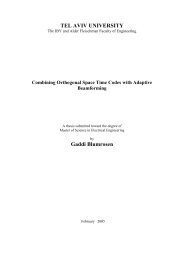
<strong>3D</strong> <strong>Motion</strong> <strong>tracking</strong><br />
<strong>with</strong> <strong>Gyroscope</strong> <strong>and</strong><br />
<strong>Accelerometer</strong><br />
Final Project<br />
By:<br />
Shay Reuveny<br />
Maayan Zadik<br />
Supervisor:<br />
Gaddi Blumrosen<br />
(Boris Rubinsky)
Table of Contents<br />
1. Introduction .......................................................................................................................................... 3<br />
2. System model ........................................................................................................................................ 5<br />
2.1 System components ...................................................................................................................... 5<br />
2.2 <strong>Accelerometer</strong> principles .............................................................................................................. 5<br />
2.3 <strong>Gyroscope</strong> principles ..................................................................................................................... 6<br />
2.3.1 Introduction .......................................................................................................................... 6<br />
2.3.2 Terms ........................................................................................................................................... 6<br />
2.3.3 The physical principles of vibrating structure gyroscope ............................................................ 7<br />
2.3.4 The mechanics of vibrating structure gyroscope ......................................................................... 8<br />
2.3.2 <strong>Gyroscope</strong> mathematical model ........................................................................................... 9<br />
3. Implementation .................................................................................................................................. 12<br />
3.1 HW Implementation ................................................................................................................... 12<br />
3.1.1 BSN node .................................................................................................................................... 12<br />
3.1.2 Types of <strong>Gyroscope</strong> ............................................................................................................. 13<br />
3.1.3 Supporting Circuit Board ..................................................................................................... 15<br />
3.2 SW implementation .................................................................................................................... 16<br />
3.2.1 Boot Sequence ........................................................................................................................... 16<br />
3.2.2 Driver for <strong>Gyroscope</strong> .................................................................................................................. 17<br />
3.2.4 Algorithm implementation ................................................................................................. 21<br />
3.2.5 GUI ...................................................................................................................................... 22<br />
4. Results <strong>and</strong> Conclusions ...................................................................................................................... 22<br />
4.1 Calibration Testing ...................................................................................................................... 22<br />
4.2 <strong>Accelerometer</strong>’s Filter Testing .................................................................................................... 23<br />
4.3 Gyro Hardware Testing ............................................................................................................... 24<br />
4.4 Route Tracking ............................................................................................................................ 24
1. Introduction<br />
In our project we use an existing "Body Sensors Network" system<br />
called BSNv3, which contains a CPU, a radio transceiver <strong>and</strong> a <strong>3D</strong><br />
accelerometer.<br />
In order to correct the results given by the accelerometer, since an<br />
accelerometer cannot detect motion <strong>with</strong> constant speed or turns,<br />
<strong>and</strong> to receive additional information about the motion in the <strong>3D</strong><br />
space, we add two dual-axis gyroscopes, which give information<br />
about all 3 axes.<br />
Figure 1.1 BSN Kit<br />
A wireless module, containing all the sensors <strong>and</strong> mounted upon the subject, will send the<br />
information to another, remote, module which is connected to a PC, using the radio transceiver<br />
of the BSN node.<br />
The information sent from the accelerometer <strong>and</strong> the gyroscopes will be combined in real-time<br />
using an algorithm which we will choose <strong>and</strong> implement, <strong>and</strong> will give us the overall info about<br />
the motion.<br />
The analyzed data will be displayed graphically on a GUI, in order to make the data readable<br />
<strong>and</strong> underst<strong>and</strong>able.<br />
Figure 1.2 An illustration of the module sending data to the remote computer
Research goals:<br />
Our goal is to assess continuous motion <strong>with</strong> a <strong>3D</strong> accelerometer <strong>and</strong> a combined <strong>3D</strong><br />
gyroscope, <strong>and</strong> make it as accurate as possible.<br />
This will be of future use in medical or educational application, such as determining the severity<br />
of Parkinson's disease, monitoring the healing process of a damaged limb, or detecting a<br />
"proper" movement in sports.<br />
Figure 1.3 The complete module
2. System model<br />
2.1 System components<br />
Our system consists of four modules:<br />
1. One remote wireless BSNv3 nodes, <strong>with</strong> a CPU <strong>and</strong> a radio transceiver.<br />
2. A <strong>3D</strong> accelerometer mounted on a BSN sensor board <strong>and</strong> connected to the BSN node.<br />
3. Two dual-axis gyroscopes, XY <strong>and</strong> XZ, mounted on an additional 'prototype' sensor board supplied<br />
<strong>with</strong> the BSNv3 kit, <strong>and</strong> also connected to the BSN node.<br />
4. A Telos-B module, which is connected to a PC <strong>and</strong> receives the data sent by the remote BSN node,<br />
sending it to the computer for further analysis.<br />
2.2 <strong>Accelerometer</strong> principles<br />
As is his name, accelerometer measures acceleration, a.<br />
<strong>Accelerometer</strong>s can measure in one, two, or three orthogonal axes. They are typically used in one of<br />
three modes:<br />
� As an inertial measurement of velocity <strong>and</strong> position<br />
� As a sensor of inclination, tilt, or orientation in 2 or 3 dimensions, as referenced from the<br />
acceleration of gravity (1 g = 9.8m/s 2 );<br />
� As a vibration or impact (shock) sensor.<br />
The most common acceleration is as a result of the earth's gravitational pull. Since it's difficult to<br />
measure acceleration directly, the accelerometer measures the force exerted by restraints placed on a<br />
reference mass to hold its position fixed in an accelerating body.<br />
When looking for <strong>and</strong> working <strong>with</strong> an accelerometer it's important to know its type of output. In both<br />
analog <strong>and</strong> digital accelerometer the output value is a scalar corresponding to the magnitude of the<br />
acceleration vector.<br />
Analog accelerometers output a constant variable voltage depending on the amount of acceleration<br />
applied. The signal can be a positive or negative voltage, depending on the direction of the acceleration.<br />
(2.1)
Since the output of this type of accelerometer will be fed to an ADC, the value must be scaled <strong>and</strong>/or<br />
amplified to maximally span the range of acquisition.<br />
Digital accelerometers output a variable frequency square wave, a method known as pulse-width<br />
modulation (PWM). A PWM accelerometer takes readings at a fixed rate.<br />
<strong>Accelerometer</strong>s <strong>with</strong> PWM output can be used in two different ways. For most accurate results, the<br />
PWM signal can be input directly to a microcontroller where the duty cycle is read in firmware <strong>and</strong><br />
translated into a scaled acceleration value. When a microcontroller <strong>with</strong> PWM input is not available, a<br />
simple RC reconstruction filter can be used to obtain an analog voltage proportional to the acceleration.<br />
These voltages can then be scaled <strong>and</strong> used as one might the output voltage of an analog output<br />
accelerometer.<br />
2.3 <strong>Gyroscope</strong> principles<br />
<strong>Gyroscope</strong> measures angular velocity, w. An angular rate gyroscope is a device that produces a positivegoing<br />
output voltage for counter-clockwise rotation around the sensitive axis considered.<br />
2.3.1 Introduction<br />
A gyroscope is a device used primarily for navigation <strong>and</strong> measurement of angular velocity expressed in<br />
Cartesian coordinates. It produces a positive-going output voltage for counter-clockwise rotation around<br />
the sensitive axis considered. There are gyroscopes available that can measure rotational velocity in 1, 2,<br />
or 3 directions. A 3-axis gyroscope combined <strong>with</strong> a 3-axis accelerometer provides a full 6 degree-offreedom<br />
(DoF) motion <strong>tracking</strong> system.<br />
2.3.2 Terms<br />
Vibrating Structure <strong>Gyroscope</strong>s are MEMS (Micro-machined Electro-Mechanical Systems) devices that<br />
are easily available commercially, affordable, <strong>and</strong> very small in size.<br />
<strong>Gyroscope</strong> Sensitivity describes the gain of the sensor <strong>and</strong> can be determined by applying a defined<br />
angular velocity to it.<br />
Zero-rate level describes the actual output signal if there is no angular rate present. The zero-rate level<br />
of precise MEMS sensors is, to some extent, a result of stress to the sensor <strong>and</strong> therefore zero-rate level<br />
can slightly change after mounting the sensor onto a printed circuit board or after exposing it to<br />
extensive mechanical stress.
Measurement range specifies the maximum angular speed <strong>with</strong> which the sensor can measure, <strong>and</strong> is<br />
typically in degrees per second (˚/sec).<br />
Number of sensing axes is the number of axes in which the gyroscope measures the angular rotation.<br />
<strong>Gyroscope</strong>s are available that measure either in one, two, or three axes. Multi-axis sensing gyros have<br />
multiple single-axis gyros oriented orthogonal to one another.<br />
Nonlinearity is a measure of how close to linear the outputted voltage is proportional to the actual<br />
angular rate. Not considering the nonlinearity of a gyro can result in some error in measurement.<br />
Nonlinearity is measured as a percentage error from a linear fit over the full-scale range, or an error in<br />
parts per million (ppm).<br />
Working temperature range specifies the temperature range in which the gyroscope works correctly<br />
<strong>and</strong> fails beyond that.<br />
Shock survivability specifies how much force the gyroscope can <strong>with</strong>st<strong>and</strong> before failing. Fortunately<br />
gyroscopes are very robust, <strong>and</strong> can <strong>with</strong>st<strong>and</strong> a very large shock (over a very short duration) <strong>with</strong>out<br />
breaking. This is typically measured in g’s (1g = earth’s acceleration due to gravity), <strong>and</strong> occasionally the<br />
time <strong>with</strong> which the maximum g-force can be applied before the unit fails is also given.<br />
B<strong>and</strong>width typically measures how many measurements can be made per second. Thus the gyroscope<br />
b<strong>and</strong>width is usually quoted in Hz.<br />
Bias is the signal output from the gyro when it is NOT experiencing any rotation. Bias can be expressed<br />
as a voltage or a percentage of full scale output, but essentially it represents a rotational velocity (in<br />
degrees per second). Unfortunately bias error tends to vary, both <strong>with</strong> temperature <strong>and</strong> over time. The<br />
bias error of a gyro is due to a number of components: Individual measurements of bias are also<br />
affected by noise, which is why a meaningful bias measurement is always an averaged series of<br />
measurements.<br />
Bias Drift refers to the variation of the bias over time, assuming all other factors remain constant. This<br />
effect is caused by the self heating of the gyroscope <strong>and</strong> its associated mechanical <strong>and</strong> electrical<br />
components. This effect would be expected to be more prevalent over the first few seconds after<br />
switch-on <strong>and</strong> to be almost non-existent after about five minutes.<br />
Bias Instability is a fundamental measure of the 'goodness' of a gyroscope. It is defined as the minimum<br />
point on the Allan Variance curve, usually measured in °/hr. It represents the best bias stability that<br />
could be achieved for a given gyro, assuming that bias averaging takes place at the interval defined at<br />
the Allan Variance minimum.<br />
2.3.3 The physical principles of vibrating structure gyroscope<br />
Fundamental to an underst<strong>and</strong>ing of the operation of a vibrating structure gyroscope is an<br />
underst<strong>and</strong>ing of the Coriolis force. In a rotating system, every point rotates <strong>with</strong> the same rotational
velocity. As one approaches the axis of rotation of the system, the rotational velocity remains the same,<br />
but the speed in the direction perpendicular to the axis of rotation decreases. Thus, in order to travel in<br />
a straight line towards or away from the axis of rotation while on a rotating system, lateral speed must<br />
be either increased or decreased in order to maintain the same relative angular position (longitude) on<br />
the body.<br />
Where is angular acceleration <strong>and</strong> m is the mass of the object whose longitude is to be<br />
maintained<br />
The Coriolis force is proportional to both the angular velocity of the rotating object <strong>and</strong> the velocity of<br />
the object moving towards or away from the axis of rotation.<br />
2.3.4 The mechanics of vibrating structure gyroscope<br />
Vibrating structure gyroscopes contain a micro-machined mass which is connected to an outer housing<br />
by a set of springs. This outer housing is connected to the fixed circuit board by a second set of<br />
orthogonal springs.<br />
The mass is continuously driven sinusoidally along the first set of springs. Any rotation of the system will<br />
induce Coriolis acceleration in the mass, pushing it in the direction of the second set of springs. As the<br />
mass is driven away from the axis of rotation, the mass will be pushed perpendicularly in one direction,<br />
<strong>and</strong> as it is driven back toward the axis of rotation, it will be pushed in the opposite direction, due to the<br />
Coriolis force acting on the mass.<br />
The Coriolis force is detected by capacitive sense fingers that are along the mass housing <strong>and</strong> the rigid<br />
structure. As the mass is pushed by the Coriolis force, a differential capacitance will be detected as the<br />
sensing fingers are brought closer together. When the mass is pushed in the opposite direction,<br />
different sets of sense fingers are brought closer together; thus the sensor can detect both the<br />
magnitude <strong>and</strong> direction of the angular velocity of the system.<br />
(2.2)<br />
Figure 2.1 A single-axis vibrating structure gyroscope schema
The first problem pending was which gyroscope to choose, since the BSN kit had 3 interfaces to<br />
which we could attach extra sensors.<br />
2.3.2 <strong>Gyroscope</strong> mathematical model<br />
A gyroscope is a device used primarily for navigation <strong>and</strong> measurement of angular velocity expressed in<br />
Cartesian coordinates:<br />
It produces a positive-going output voltage for counter-clockwise rotation around the sensitive axis<br />
considered. The coordinates are of Inertial Axes (or Body Axes) - based on Center of Gravity (CG)<br />
The body axes positions are:<br />
� X Axis - Positive forward, through the nose of the object<br />
� Y Axis - Positive to Right of X Axis, perpendicular to X Axis<br />
� Z Axis - Positive downwards, perpendicular to X-Y plane<br />
The Angles definitions are:<br />
(2.3)<br />
� Pitch - Angle of X Axis relative to horizon. Also a positive rotation about Y Body Axis<br />
� Roll - Angle of Y Axis relative to horizon. Also a positive rotation about X Body Axis<br />
� Yaw - Angle of X Axis (nose) relative to North. Also a positive rotation about Z Body axis<br />
22.2 The angular rotation of an airoplain
The angle can be derived by integration of the angular velocity in each direction:<br />
Where p is index which can be (x,y,z ), Pitch is , Roll is <strong>and</strong> Yaw is <strong>and</strong> is the initial angle<br />
compared to the earth axis.<br />
(2.4)<br />
In many times we need to work <strong>with</strong> earth Axis coordinates which are defined as follow:<br />
� X Axis - Positive in the direction of North<br />
� Y Axis - Positive in the direction of East (perpendicular to X Axis)<br />
� Z Axis - Positive towards the centre of Earth (perpendicular to X-Y Plane)<br />
In order to convert from body axes to earth axes we use the following matrix:<br />
Where is the roll around the x-axis, is the pitch around the y-axis <strong>and</strong> is the yaw around the z-<br />
axis, as shown below:<br />
Figure 2.3 The angular rotation of an airoplain<br />
Figure 2.4 Body to earth example<br />
The matrix is used to convert the angles from angles referring to the body’s movement from its previous<br />
position, to angles referring to its movement from the position before it. When it is then multiplied <strong>with</strong>
all the previous matrixes, since each matrix represents one movement, the multiplied outcome<br />
represents all the movements since the beginning of the measurements, thus multiplying the body axes<br />
coordinates, *Xb, Yb, Zb+, <strong>with</strong> the above mentioned matrix, will result in the object’s coordinates in<br />
earth axes.
3. Implementation<br />
3.1 HW Implementation<br />
3.1.1 BSN node<br />
BSN node consists of a CPU, A flash memory <strong>and</strong> a radio transceiver.<br />
In order to connect to additional sensors it has analog <strong>and</strong> digital interfaces:<br />
Analog interface<br />
1. An analog interface – The CPU on the main board has several ADC pins to which analog<br />
devices can be connected.<br />
2. It has 8 ADC's (ADC0 to ADC7) to connect the analog sensor output, together <strong>with</strong><br />
'SESOR_PWR' <strong>and</strong> 'GND' pins that can supply the power <strong>and</strong> the ground for the sensor.<br />
3. As for the actual connection, it can be made by extra 2 ADC's (ADC4 to ADC5) on the board<br />
containing the accelerometer, or by the "Prototype" board available <strong>with</strong> the kit,<br />
Digital interface<br />
1. A Digital I2C Interface – An I2C interface is a serial bus interface that uses the I2C protocol. A<br />
sensor that uses that interface can be connected to the kit's 'Prototype' board through the<br />
'SENSOR_SCL' <strong>and</strong> 'SENSOR_SDA' pins that connect to the I2C clock signal <strong>and</strong> to the data<br />
signal respectively, <strong>and</strong> also to the power <strong>and</strong> ground pins as the analog sensors.<br />
2. A Digital UART/RS232 Interface – A sensor <strong>with</strong> a UART interface can be connected to the<br />
'UART1TX' <strong>and</strong> 'UART1RX' pins on the 'Prototype' board, or by a BSN Serial interface board,<br />
that is supplied separately from the kit.<br />
Pros<br />
Cons<br />
� Synchronized, own power<br />
regulations.<br />
Digital Analog<br />
� Different usage from the<br />
accelerometer - which is analog<br />
� There is only one set of I2C/UART<br />
clock <strong>and</strong> data pins – we would need<br />
another board to use 2 gyroscopes.<br />
� Not widely available.<br />
3.1 Digital VS. Analog gyroscope<br />
� Simple, operation same as accelerometer.<br />
� Prototype board has 8 available ADC pins –<br />
can connect more than one gyroscope.<br />
� More sensitivity <strong>and</strong> range choices.<br />
� Not synchronized.<br />
� Have to regulate power supply ourselves.<br />
� Have to translate results to valid data.
3.1.2 Types of <strong>Gyroscope</strong><br />
From the various websites <strong>and</strong> companies we found that supply gyroscopes or full motion sensors<br />
containing a gyroscope, the three most prominent ones that were suitable for our needs were the<br />
"Analog-Devices", "Invensence" <strong>and</strong> "STMicroelectronics" company websites.<br />
3-D gyroscope is not available yet.<br />
1. 'Analog Devices' Gyros<br />
http://www.analog.com/en/mems/gyroscopes/products/index.html<br />
The Analog-Devices company supplies gyroscopes <strong>with</strong> an analog or digital interfaces, but almost all<br />
of them are 1-axis gyroscopes, <strong>and</strong> since we were looking for a tri-axis one, is was not good for us.<br />
This company did have a tri-axis gyroscope, but it was a part of a kit that costs about 320$, so we<br />
looked for other solutions.<br />
2. 'Invensence' Gyros<br />
http://www.invensense.com/store/index.html<br />
The Invensence company supplies gyroscopes using the I2C interface, that we can use to connect<br />
them to the BSN board, <strong>and</strong> are also cheap in comparison to other gyroscopes we encountered<br />
(around 9$ per piece). Although the online store in the above mentioned website displayed only 1axis<br />
<strong>and</strong> dual-axis gyroscopes available for purchase, we found an article in another website<br />
claiming that the company is about to launch a new tri-axis gyroscope, the ITG-3200 gyro chip, that<br />
is the first of its kind <strong>and</strong> costs only 3$ per piece.<br />
After a short correspondent <strong>with</strong> the Invensence's sales department, we learned that this chip will<br />
only be available on the 3rd quarter of 2010, which is by far too late for our schedule.<br />
We also looked at a digital dual-axis gyroscope, IDG-2000. According to the company site, The IDG-<br />
2000 is the first digital gyro <strong>with</strong> both SPI <strong>and</strong> I2C interfaces, <strong>and</strong> is available in Pitch <strong>and</strong> Roll (X,Y)<br />
<strong>and</strong> Pitch <strong>and</strong> Yaw (X,Z) configurations.<br />
If we were to use this gyroscope, we would have to figure out how exactly to connect the two<br />
separate gyroscopes to the BSN kit. Since the Prototype board has only one I2C clock <strong>and</strong> data pins,<br />
we were wondering if we can connect both gyros to the same pins in the same Prototype board, or<br />
do we actually need one more Prototype board, se we will connect each gyro to a separate board,<br />
<strong>and</strong> use the BSN board's bus behavior to distinguish between the two.<br />
According to the press release on September 8, 2009, the IDG-2000 MEMS gyroscopes began<br />
sampling on October 2009 to selected OEM partners. It is not available yet to the public.<br />
We then turned to looking at 2 analog dual-axis gyroscopes, a Pitch <strong>and</strong> Roll (X,Y) <strong>and</strong> a Pitch <strong>and</strong><br />
Yaw (X,Z) gyros.<br />
In order to use two compatible gyros of the same specifications, we could chose either the IDG-500<br />
(X,Y) <strong>and</strong> the IXZ-500 (X,Z) gyros, both <strong>with</strong> a sensitivity of 2 mV/°/sec Primary output <strong>and</strong> 9.1<br />
mV/°/sec Secondary output, <strong>and</strong> a full scale range of ± 500 °/sec, or the IDG-650 <strong>and</strong> IXZ-650, <strong>with</strong> a<br />
sensitivity of 0.5 mV/°/sec Primary output <strong>and</strong> 2.27 mV/°/sec Secondary output, <strong>and</strong> a full scale<br />
range of ± 2000 °/sec.<br />
3. STMicroelectronics Gyros
Company<br />
http://www.st.com/stonline/products/families/sensors/gyroscopes.html<br />
The STMicroelectronics website, which we found recently, provides us <strong>with</strong> the same solution as<br />
the Invensence website, which is to use 2 dual-axis gyros. As opposed to the Invensence gyros, this<br />
site offers analog output dual-axis gyros, <strong>with</strong> broader selection <strong>and</strong> the same specifications as the<br />
Invensence gyros, but no prices were presented on the website. The broader selection may be an<br />
advantage to us since we can choose a more appropriate gyro for our needs.<br />
Since we need 2 gyros, we will have to connect both of them to the Prototype board, i.e. to the ADC<br />
pins available, together <strong>with</strong> SENSOR_PER <strong>and</strong> GND.<br />
These gyroscopes have self-test, ST, <strong>and</strong> sleep /power down, SLEEP/PD, pins, that we can use to set<br />
the gyroscopes to sleep when they are not in use, <strong>and</strong> using all analog sensors (gyroscopes <strong>and</strong><br />
accelerometer) might help us to better synchronize the results.<br />
Analog<br />
Or<br />
Digital<br />
InvenSence Analog<br />
STM Analog<br />
Product<br />
Number<br />
Axes<br />
Sensitivity<br />
[mV/dps]<br />
Low High<br />
Range<br />
[dps]<br />
High Low<br />
Price<br />
[$]<br />
Power<br />
[mW]<br />
P=V∙I<br />
Operation<br />
Voltage<br />
[V]<br />
B<strong>and</strong>width<br />
[Hz]<br />
IDG-500<br />
IDG-650<br />
XY<br />
2<br />
0.5<br />
9.1<br />
2.27<br />
±500<br />
±2000<br />
±110<br />
±440<br />
9.00<br />
9.00<br />
21<br />
21<br />
3.0±10%<br />
3.0±10%<br />
NA<br />
NA<br />
IXZ-500<br />
IXZ-650<br />
XZ<br />
2<br />
0.5<br />
9.1<br />
2.27<br />
±500<br />
±2000<br />
±110<br />
±440<br />
9.00<br />
9.00<br />
21<br />
21<br />
3.0±10%<br />
3.0±10%<br />
NA<br />
NA<br />
LPR403AL/<br />
LPR503AL<br />
8.3 33.3 ±120 ±30<br />
4.62-<br />
6.05<br />
20.4 3.0±10% 140<br />
LPR410AL/<br />
LPR510AL<br />
2.5 10 ±400 ±100<br />
4.62-<br />
6.05<br />
20.4 3.0±10% 140<br />
LPR430AL/<br />
LPR530AL<br />
XY 0.83 3.33 ±1200 ±300<br />
4.62-<br />
6.05<br />
20.4 3.0±10% 140<br />
LPR450AL/<br />
LPR550AL<br />
0.5 2 ±2000 ±500<br />
4.62-<br />
6.05<br />
20.4 3.0±10% 140<br />
LPR4150AL/<br />
LPR5150AL<br />
0.67 0.167 ±6000 ±1500 4.62-<br />
6.05<br />
20.4 3.0±10% 140<br />
LPY403AL/<br />
LPY503AL<br />
8.3 33.3 ±120 ±30<br />
4.62-<br />
6.05<br />
20.4 3.0±10% 140<br />
LPY410AL/<br />
LPY510AL<br />
2.5 10 ±400 ±100<br />
4.62-<br />
6.05<br />
20.4 3.0±10% 140<br />
LPY430AL/<br />
LPY530AL<br />
XZ 0.83 3.33 ±1200 ±300<br />
4.62-<br />
6.05<br />
20.4 3.0±10% 140<br />
LPY450AL/<br />
LPY550AL<br />
0.5 2 ±2000 ±500<br />
4.62-<br />
6.05<br />
20.4 3.0±10% 140<br />
LPY4150AL/<br />
LPY5150AL<br />
0.67 0.167 ±6000 ±1500 4.62-<br />
6.05<br />
20.4 3.0±10% 140<br />
Table 3.2 <strong>Gyroscope</strong> comparison <strong>and</strong> specifications
The battery given to us by the BSN kit supplies +3.7V <strong>and</strong> 55mAh. After a quick calculation we concluded<br />
that the battery will last almost 10 hours.<br />
From the different kinds of gyroscopes existing, we're going to use a Vibrating Structure <strong>Gyroscope</strong>s,<br />
which are MEMS (Micro-machined Electro-Mechanical Systems) devices that are easily available<br />
commercially, affordable, <strong>and</strong> very small in size.<br />
We chose to order STMicroelectronics’ LPR510AL <strong>and</strong> LPY510AL gyroscopes because they are small,<br />
cheaper than InvenSence’s <strong>and</strong> their range/sensitivity is best for our use. Furthermore, if at any time we<br />
discover that the range (in amplified mode) is too narrow for us we can always use the wider range<br />
(regular mode), giving us room for error <strong>and</strong> changes in our initial estimate.<br />
We prefer sensitivity over range as our problem does not change in wide angles.<br />
3.1.3 Supporting Circuit Board<br />
In order to connect the gyroscopes to the BSN Kit, we needed to build a supporting circuit board,<br />
connect it to the appropriate gyroscope pins <strong>and</strong> connect them to the BSN prototype board. According<br />
to the gyroscope data sheet, there are 3 circuits needed for each gyroscope:<br />
Figure 3.1 The gyroscope’s electrical specifications
The red circuits, which are identical, are low-pass filters for the X <strong>and</strong> Y outputs, as displayed in the<br />
figure. They connect between the non-amplified output <strong>and</strong> the amplified input, while reducing the<br />
outputted noise. The amplified inputs are internally connected to the amplified outputs, from which we<br />
take our results.<br />
The green circuit provides a low-pass filter for the gyroscope's internal synchronization mechanism.<br />
The blue circuit provides voltage stabilization for the voltage supply pin.<br />
Figure 3.2 depicts the board we designed <strong>and</strong> built, containing all the needed circuits for both<br />
gyroscopes. This board, together <strong>with</strong> the board containing the sensors, connects as a complete<br />
gyroscope module to the BSN prototype board.<br />
3.2 SW implementation<br />
3.2.1 Boot Sequence<br />
Figure 3.2 Supporting board design
The TinyOS platform, that we are using, had a distinct boot sequence that comprises of 3 steps:<br />
1. INITIALIZE SCHEDULER.<br />
2. INITIALIZE PLATFORM AND SOFTWARE.<br />
3. SIGNAL THE PROGRAM THAT THE HARDWARE HAS BEEN INITIALIZED.<br />
This initialization is made in the main module of the TinyOS, which is comprised of a configuration file<br />
'MainC.nc', <strong>and</strong> a component 'RealMainP.nc', which contains the main() method.<br />
Each platform (e.g. micaz, telos, BSNv3) has a unique implementation of the platform initialization,<br />
defined in a configuration module called 'PlatformC.nc', which every new platform that wishes to use<br />
TinyOS has to supply.<br />
The Main() method calls a 'PlatformInit.init()' function, that is implemented <strong>and</strong> wired to the<br />
'PlatformC.nc' component.<br />
This method, in collaboration <strong>with</strong> a platform-unique 'hardware.h' file, connects the pins of the chips it<br />
is using to the appropriate outputs <strong>and</strong> inputs.<br />
Main(){<br />
RealMainP.nc<br />
call Scheduler.init();<br />
call PlatformInit.init();<br />
call SoftwareInit.init();<br />
signal Boot.booted();<br />
Hardware.h<br />
PlatformC.nc<br />
Init()<br />
Figure 3.3 TinyOS platform based boot sequence<br />
For the accelerometer board supplied <strong>with</strong> the BSNv3 node, a 'BSNv<strong>3D</strong>evKitsb' in defined in the TinyOS<br />
'sensorboard' directory, which supplies the interface for accessing the accelerometer's readings. The<br />
board is connected to the mote in it's make target file, 'bsnv3.target' by the assignment:<br />
"SENSORBOARD ?= BSNv<strong>3D</strong>evKitsb".<br />
We will add our new sensor board to the configuration or merge it <strong>with</strong> the existing accelerometer<br />
sensor board.<br />
3.2.2 Driver for <strong>Gyroscope</strong>
For each sensor board that is used in the platform, a configuration <strong>and</strong> module .nc files are written for<br />
the various sensors the board contains, <strong>and</strong> a general module implementation, that ties all of them<br />
together.<br />
In our case, since we need to add two gyroscopes, an XY gyro <strong>and</strong> an XZ gyro, we will have to create two<br />
modules:<br />
GyroXYC.nc, GyroXYM.nc<br />
GyroXZC.nc, GyroXZM.nc<br />
Each configuration file (*C.nc) provides two 'Read' interfaces, one for each axis. This interface<br />
consists of two methods:<br />
1. comm<strong>and</strong> error_t read();<br />
(Basically a true/false specifying if new data is available)<br />
2. event void readDone(value);<br />
(Copies the data received to the specified 'value' variable)<br />
These interfaces are wired to a built in module written for receiving data from the ADC's, called<br />
'AdcReadClientC()'. Note that the actual method for reading from the ADC already exists, <strong>and</strong> we will<br />
wire it to our new components.<br />
GyroXYC.nc<br />
AdcReadClientC() as GyroX;<br />
AdcReadClientC() as GyroY;<br />
GyroXZC.nc<br />
AdcReadClientC() as GyroX;<br />
AdcReadClientC() as GyroZ;<br />
AdcReadClientC<br />
Figure 3.4 new gyro modules <strong>with</strong> wired interface<br />
Read<br />
comm<strong>and</strong> error_t read();<br />
event void readDone(value);<br />
Each *M.nc file contains a configuration for each axis, that define the input channels for the sensor, in<br />
addition to other element necessary for reading. These are wired to the ADC client's configuration<br />
Interface, called 'AdcConfigure', by each gyro's configuration module.
AdcReadClientC<br />
AdcConfigure<br />
GyroXYM.nc<br />
AdcConfigure as ConfigX;<br />
AdcConfigure as ConfigY;<br />
GyroXZM.nc<br />
AdcConfigure as ConfigX;<br />
AdcConfigure as Configz;<br />
Figure 3.5 ADC configuration for each axis in each gyro<br />
Another module, BSNv3<strong>3D</strong>Gyro(C/M).nc, will combine the ReadX, ReadY <strong>and</strong> ReadZ from the two other<br />
modules <strong>and</strong> will supply a full <strong>3D</strong> gyro interface, which we can then use for our programs. It will also<br />
implement 'StdControl' start <strong>and</strong> stop methods, which regulate the power for the whole sensor board.<br />
BSNv3<strong>3D</strong>GyroM.nc<br />
Read as GyroX1<br />
Read as GyroY<br />
Read as GyroX2<br />
Read as GyroZ<br />
StdControl<br />
3.2.3 Conversion & Filtering<br />
3.2.3.1 Calibration<br />
GyroXYC.nc<br />
GyroXZC.nc<br />
Figure 3.6 An overall module that supplies the full <strong>3D</strong> interface<br />
Since the accelerometer's output is influenced by the supplied voltage <strong>and</strong> battery power, there<br />
is a need to calibrate the accelerometer prior to use in order to get more accurate results.<br />
For this purpose, we wrote an automatic calibration program using Matlab. For each axis, the<br />
program measures the accelerometer's output in zero <strong>and</strong> g gravity, <strong>and</strong> calculates the average<br />
over a given amount of output samples. This is done in order to compensate for the unstable<br />
measurements given by the accelerometer.
By assuming that the acceleration is linear, we can use a linear equation system to extract the<br />
actual acceleration from the output given by the accelerometer.<br />
Using the averaged measurement results in each gravitational situation, we dem<strong>and</strong> that:<br />
- the accelerometer's output samples in zero gravity.<br />
- the accelerometer's output samples in g gravity.<br />
The program calculates the coefficients for each one of the axes, <strong>and</strong> saves them. We can later<br />
use these coefficients to them to determine the actual acceleration by calculating:<br />
3.2.3.2 Filters <strong>and</strong> Corrections<br />
The accelerometer’s unstable measurements forced us to implement an adaptable Gaussian filter, in<br />
order to get smoother results.<br />
The adaptable filter is composed of 6 Gaussian filters, scaling from the size of 5 to the size of 15<br />
elements, where every filter is a weighted average of the current sample, FILTER_SIZE/2 samples before<br />
it <strong>and</strong> FILTER_SIZE/2 samples after it, <strong>and</strong> more weight is given to the elements closer to the current<br />
sample.<br />
The filter size grows when we see consistency <strong>and</strong> shrinks back to 5 when we detect a drastic change in<br />
the acceleration.<br />
As we reviewed the accelerometer’s output, we noticed that there are sometimes spikes in the results,<br />
that make it look as though the object is accelerating more than it actually does. This phenomenon<br />
happens once in a few samples, so we can pinpoint when it happens by comparing the sample’s value<br />
<strong>with</strong> its neighbors’ average.<br />
(3.1)<br />
(3.2)
When the distance between the two compared values exceeds 0.2 <strong>and</strong> the distance between the<br />
current sample’s value <strong>and</strong> its previous’ value exceeds what we conceive as a normal acceleration pace,<br />
we consider the value in question a spike, ignore it, <strong>and</strong> replace it <strong>with</strong> its neighbors’ average. If we<br />
consider the current sample’s successor a spike as well, we will replace it <strong>with</strong> the value of its previous.<br />
Figure 3.7 The pseudo code for the spike removal filter (where X is the samples buffer)<br />
Due to the fact that our accelerometer uses the earth’s gravitational force to identify acceleration, when<br />
our module is not held directly parallel to the X <strong>and</strong> Y axes, the gravity affects the accelerometer’s<br />
measurements, <strong>and</strong> we receive a false indication of acceleration.<br />
In order to negate the gravity’s affect, we need to keep track of the current angle of our moving body in<br />
accordance to the X <strong>and</strong> Y axes. When we receive an acceleration reading, we check our current angle<br />
<strong>and</strong> using simple trigonometry, calculate the exact offset of acceleration caused by gravity. We then<br />
subtract this offset from our reading in order to receive the real acceleration of the body.<br />
3.2.4 Algorithm implementation<br />
We implemented our algorithm using the Matlab software. The algorithm envelopes all the<br />
steps, starting <strong>with</strong> receiving the measurements, <strong>and</strong> ending <strong>with</strong> the display of the route.<br />
3.2.4.1 Receiving the data<br />
Receiving the raw data, calculating the measurements <strong>and</strong> storing them in appropriate buffers.<br />
3.2.4.2 Filtering the measurements<br />
The accelerometer’s measurements are filtered for spikes <strong>and</strong> smoothed <strong>with</strong> the Gaussian<br />
Filter, as detailed in the filtering section (3.2.4.2).<br />
The results of the gyroscope are also filtered using a basic averaging filter.<br />
3.2.4.3 Converting the angular velocity measured by the gyroscope
The gyroscope measures the angular velocity in each direction, during the sample interval. In<br />
order to obtain the new angles, we use the following equation, for each coordinate:<br />
3.2.4.4 Converting to earth coordinates<br />
(3.3)<br />
Implementing matrix <strong>and</strong> calculation as explained in section 2.3.2, that results in [X,Y,Z]<br />
coordinates in relation to earth axes.<br />
3.2.4.5 Compensating for gravity<br />
Extracting the current angle of the object in relation to earth’s X <strong>and</strong> Y axes, computing the<br />
affects of the gravity on the accelerometer’s measurement, <strong>and</strong> reducing it from the<br />
acceleration we calculated previously.<br />
3.2.4.6 Calculating the progress vector<br />
Calculating the distance the object traveled in that time interval, using the accelerometer’s<br />
measurements, calculating the direction of progress using the angles previously calculated, <strong>and</strong><br />
combining the two to extract the progress vector.<br />
3.2.4.7 Displaying the results<br />
3.2.5 GUI<br />
We use the Matlab application to run our algorithm <strong>and</strong> display the results graphically using its ‘Figure’<br />
tools. After analyzing the data <strong>and</strong> calculating the object’s current position, we’ll display the course the<br />
object makes in real-time.<br />
4. Results <strong>and</strong> Conclusions<br />
4.1 Calibration Testing<br />
As showed in section 3.2.3.1, we calibrated the accelerometer’s data before we started the test its<br />
measurements.<br />
The results we received at first, before the calibration was done, were inaccurate. The inaccuracy was
caused by the measurements’ drift, resulted from internal heating <strong>and</strong> the accelerometer’s mechanism,<br />
<strong>and</strong> also by inconsistent readings, even when the module was stationary.<br />
These circumstances brought us to choose to calibrate the accelerometer, after which the accuracy of<br />
our results improved immensely.<br />
X<br />
Y<br />
Min Max Avg. Delta<br />
4.2 <strong>Accelerometer</strong>’s Filter Testing<br />
Table 4.1 results of calibration<br />
We looked at the accelerometer‘s readings for some r<strong>and</strong>om movement, <strong>and</strong> displayed the results<br />
before <strong>and</strong> after the filtering process. We did this to test if the filter works correctly.<br />
At first we applied only the Gaussian filter on the accelerometer’s results. We noticed that sometimes, a<br />
measurement spike, that falsely indicated a certain acceleration value, caused the results to chance,<br />
although the filter was applied. This alerted us to the fact that we need remove the spikes by altering<br />
the readings from the received measurement to an average of its surrounding samples.<br />
After we applied this alteration, our results were much smoother, but we noticed that sometimes spikes<br />
arrive one directly after another, causing a distortion of the filtered result. We changed the spike filter<br />
to also address this problem, <strong>and</strong> this we were content <strong>with</strong> the results, as can be seen in the figure<br />
below:<br />
Figure 4.0.1 <strong>Accelerometer</strong>’s X axes results before <strong>and</strong> after filtering
As the graphs show, after we apply the filter the results are smoother <strong>and</strong> less noisy, so we can proceed<br />
to the next level.<br />
4.3 Gyro Hardware Testing<br />
According to the gyroscope specifications sheet, we measured, using an oscilloscope, the input <strong>and</strong><br />
output voltage of the gyroscope, to make sure we receive correct readings.<br />
The input voltage the gyroscope expects in order to function correctly is between 2.7V <strong>and</strong> 3.6V. When<br />
we tested the gyroscope’s input voltage, using the oscilloscope, we noticed that the gyroscope’s supply<br />
voltage is only 2.2V. We concluded that the battery given to us <strong>with</strong> the BSN Kit doesn’t supply the<br />
required voltage to activate both gyroscope <strong>and</strong> accelerometer properly. Thus, we decided to replace<br />
the battery holder <strong>with</strong> one that holds 2 st<strong>and</strong>ard AA 1.5V batteries. After doing so we got a supplied<br />
voltage of 3V for the gyroscope, which as mentioned before is enough.<br />
When testing the output voltage of each of the gyroscope’s axes, we noticed a lot of noise, when using<br />
the oscilloscope. We then decided to replace the original 2.2nF capacitors we used in the gyroscope’s<br />
supporting board <strong>with</strong> 1uF capacitors, thus getting better results.<br />
4.4 Route Tracking<br />
In order to test that our algorithm, using the readings from the combined gyroscope <strong>and</strong> accelerometer<br />
module, is able to detect an actual route in <strong>3D</strong> space, we mounted the module on a remote controlled<br />
toy car, which we then moved in various routes, <strong>and</strong> checked whether the software correctly displayed<br />
the car’s path.<br />
Our first test was to move the car in a continuous circular movement, <strong>and</strong> check how well the route is<br />
displayed.
Figure 4.0.2 A circular route <strong>and</strong> its display via Matlab<br />
As we can see from the Matlab plot our algorithm successfully managed to identify that the car moved<br />
in a circular route.<br />
We proceeded to moving the car in different routes, each time checking if the correct path was<br />
displayed, <strong>and</strong> making small adjustments to the filters accordingly. By doing so we were able to achieve<br />
satisfying results.<br />
The following figure contains screenshots from one of these videoed tests, in which we moved the car in<br />
a r<strong>and</strong>om path, <strong>and</strong> checked the progress on the display.<br />
Figure 4.0.3 Screenshots from the video depicting the progress in Matleb’s display, as the car makes its route
Our tests were performed in a 2D space, using only one of the gyroscopes (Pitch-Yaw), but our module<br />
<strong>and</strong> software are designed to work fully well in <strong>3D</strong> space.