Solution to Homework 5
Solution to Homework 5
Solution to Homework 5
- TAGS
- www.cse.cuhk.edu.hk

You also want an ePaper? Increase the reach of your titles
YUMPU automatically turns print PDFs into web optimized ePapers that Google loves.
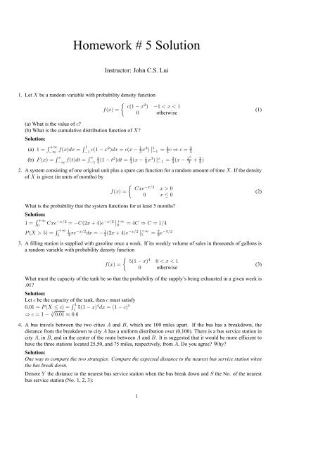
<strong>Homework</strong> # 5 <strong>Solution</strong><br />
Instruc<strong>to</strong>r: John C.S. Lui<br />
1. Let X be a random variable with probability density function<br />
�<br />
2 c(1−x ) −1 < x < 1<br />
f(x) =<br />
0 otherwise<br />
(a) What is the value of c?<br />
(b) What is the cumulative distribution function ofX?<br />
<strong>Solution</strong>:<br />
(a) 1 = � +∞<br />
−∞ f(x)dx = � 1<br />
−1 c(1−x2 )dx = c(x− 1<br />
(b) F(x) = � x<br />
−∞f(t)dt = � x 3<br />
−1 4 (1−t2 )dt = 3<br />
4<br />
3x3 ) � �1<br />
−1 = 4<br />
3<br />
(x− 1<br />
3x3 ) � �x<br />
−1 = 3<br />
4<br />
c ⇒ c = 3<br />
4<br />
(x− x3<br />
3<br />
2. A system consisting of one original unit plus a spare can function for a random amount of timeX. If the density<br />
of X is given (in units of months) by<br />
�<br />
−x/2 Cxe x > 0<br />
f(x) =<br />
(2)<br />
0 x ≤ 0<br />
What is the probability that the system functions for at least 5 months?<br />
<strong>Solution</strong>:<br />
1 = � +∞<br />
0 Cxe−x/2 = −C(2x+4)e −x/2� � +∞<br />
0 = 4C ⇒ C = 1/4<br />
P(X > 5) = � +∞<br />
5<br />
1<br />
4xe−x/2dx = −1 4 (2x+4)e−x/2� � +∞ 7<br />
5 = 2e−5/2 3. A filling station is supplied with gasoline once a week. If its weekly volume of sales in thousands of gallons is<br />
a random variable with probability density function<br />
�<br />
4 5(1−x) 0 < x < 1<br />
f(x) =<br />
(3)<br />
0 otherwise<br />
What must the capacity of the tank be so that the probability of the supply’s being exhausted in a given week is<br />
.01?<br />
<strong>Solution</strong>:<br />
Let c be the capacity of the tank, then c must satisfy<br />
0.01 = P(X ≤ c) = � 1<br />
c 5(1−x)4 dx = (1−c) 5<br />
⇒ c = 1− 5√ 0.01 ≈ 0.6<br />
4. A bus travels between the two cities A and B, which are 100 miles apart. If the bus has a breakdown, the<br />
distance from the breakdown <strong>to</strong> city A has a uniform distribution over (0,100). There is a bus service station in<br />
city A, in B, and in the center of the route between A and B. It is suggested that it would be more efficient <strong>to</strong><br />
have the three stations located 25,50, and 75 miles, respectively, fromA, Do you agree? Why?<br />
<strong>Solution</strong>:<br />
One way <strong>to</strong> compare the two strategies: Compare the expected distance <strong>to</strong> the nearest bus service station when<br />
the bus break down.<br />
Denote Y the distance <strong>to</strong> the nearest bus service station when the bus break down and S the No. of the nearest<br />
bus service station (No. 1, 2, 3):<br />
1<br />
+ 2<br />
3 )<br />
(1)
a) In the original setting that the three bus service stations numbered 1, 2, 3 are 0, 50 and 100 miles away from<br />
A:<br />
E[Y] = E[Y|S = 1]P(S = 1)+E[Y|S = 2]P(S = 2)+E[Y|S = 3]P(S = 3)<br />
� 25<br />
= ( |x−0|dx)·<br />
0<br />
25−0<br />
100 +(<br />
� 75<br />
|x−50|dx)·<br />
25<br />
75−25<br />
100 +(<br />
� 100<br />
|x−100|dx)·<br />
75<br />
100−75<br />
100<br />
= 12.5<br />
b) In the suggested setting that the three bus service stations numbered 1, 2, 3 are 25, 50 and 100 miles away<br />
from A:<br />
E[Y] = E[Y|S = 1]P(S = 1)+E[Y|S = 2]P(S = 2)+E[Y|S = 3]P(S = 3)<br />
� 37.5<br />
= ( |x−25|dx)·<br />
0<br />
37.5−0<br />
100 +(<br />
� 62.5<br />
|x−50|dx)·<br />
37.5<br />
62.5−37.5<br />
� 100<br />
+( |x−75|dx)·<br />
100 62.5<br />
100−75<br />
100<br />
≈ 10<br />
Therefore, the suggested positions are better.<br />
5. LetX be a normal random variable with mean 12 and variance 4. Find the value ofcsuch thatP{X > c} = .10.<br />
<strong>Solution</strong>:<br />
Standard trick: Transfer the normal random viable X <strong>to</strong> standard normal random viable (X −µ)/σ<br />
From textbook table 5.1, we know:<br />
Solve equation<br />
P(X > c) = P((X −12)/2 > (c−12)/2)<br />
= 1−Φ((c−12)/2)<br />
= 0.10<br />
1−Φ(1.28) ≈ 0.10<br />
1.28 = (c−12)/2c<br />
⇒ c = 14.56<br />
6. Suppose that the height, in inches, of a 25-year-old man is a normal random variable with parameters µ = 71<br />
and σ 2 = 6.25. What percentage of 25-year-old man are over 6 feet, 2 inches tall? What percentage of men in<br />
the 6-footer club are over 6 feet, 5 inches?<br />
<strong>Solution</strong>:<br />
Denote X the height of a 25-year-old man.<br />
(a) 1 foot = 12 inches, therefore 6 feet 2 inches = 74 inches<br />
(b) 6 feet = 72 inches, 6 feet 5 inches = 77 inches<br />
P(X > 74) = P((X −71)/2.5 > 1.2)<br />
= 1−Φ(1.2)<br />
= 1−0.8849 (textbook table 5.1)<br />
≈ 11.5%<br />
P(X > 77|X > 72) = P((X −77)/2.5 > 2|(X −72)/2.5 > 0.4)<br />
= (1−Φ(2))/(1−Φ(0.4))<br />
= (1−0.9861)/(1−0.6554) (textbook table 5.1)<br />
≈ 4%<br />
7. A model for the movement of a s<strong>to</strong>ck supposes that if the present price of the s<strong>to</strong>ck is s, then, after one period,<br />
it will be either us with probability p or ds with probability 1 − p. Assuming that successive movements are<br />
independent, approximate the probability that the s<strong>to</strong>ck’s price will be up at least 30 percent after the next 1000<br />
periods ifu = 1.012, d = 0.990, and p = 0.52.<br />
2
<strong>Solution</strong>:<br />
Let s be the initial price of the s<strong>to</strong>ck. Denote X the number of increase periods among the 1000 time periods. Then<br />
the price at the end is<br />
su X d 1000−X<br />
In order for thye price <strong>to</strong> be at least 1.3s, we need<br />
d 1000 ( u<br />
d )X > 1.3<br />
⇒ X > log(1.3)−1000logd<br />
log(u/d)<br />
That is, we need at least 470 increase periods.<br />
Since X is binomial with parameters 1000, 0.52, we have<br />
≈ 469.2<br />
X −1000·0.52<br />
(continuity correction here) P(X > 469.5) = P( √ ><br />
1000·0.52·0.48 469.5−1000·0.52<br />
√ )<br />
1000·0.52·0.48<br />
≈ Φ(−3.196) (The DeMoivre-Laplace limit theorem, textbook p.204)<br />
≈ 0.9993<br />
3