Salman Habib - Los Alamos National Laboratory

1998 2015 

Cosmological Simulations: 

Modeling the Universe 

Salman Habib 

Los Alamos National Laboratory 

SF09, July 10, 2009 

Visualization: Pat McCormick, 

CCS-1, LANL 

SDSS, Katrin First Heitmann, Light Los Alamos in 1998 National Laboratory Deep Lens LBNL, Survey/LSST 

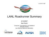
March 12, 2009

Standard Model of Cosmology and Beyond 

• Good idea of the history of the Universe 

• Good idea of the composition: 

‣ ~73% of a mysterious dark energy 

‣ ~23% of an unkown dark matter component 

‣ ~4% of baryons 

• Constraints on ~20 cosmological 

parameters, including optical depth, 

spectral index, Hubble constant, ... 

• Values are known to ~10% 

• For comparison: the parameters of the 

Standard Model of Particle Physics are 

known with 0.1% accuracy! 

• Where do we go from here? 

‣ Precision for the sake of precision not useful, 

want more theory and less phenomenology 

‣ Observations and theory must work together to 

understand the unknowns of the current 

Standard Model 

‣ What is the Dark Energy? What is the Dark 

Matter? Does GR have to be modified? Where 

do the primordial fluctuations come from? How 

can inflation be tested? (More physics and 

less scenarios) 

z~1000 

Katrin Heitmann, Los Alamos National Laboratory LBNL, March 12, 2009 

z~30 

z~2

Progress in Cosmology I: CMB 

• Cosmic microwave background 

measurements started the era of 

“precision cosmology” 

• What made it “precision”? 

‣ Physics “easy” to understand 

‣ In its wavelength band, the CMB 

dominates the sky 

• After CMB, what? 

‣ More CMB (polarization), but much 

messier! 

‣ Large scale structure probes -- but 

now must go beyond linear theory 

2009+ Planck 

Katrin Heitmann, Los Alamos National Laboratory LBNL, March 12, 2009

Progress in Cosmology II: LSS 

Void 

Gregory & Thompson, 1978 

• 1978: Discovery of voids and 

superclusters, theory of hierarchical 

structure formation via gravitational 

instability emerges 

• 2006: SDSS has measured more than 

1,000,000 galaxies, key discoveries such 

as BAO (Eisenstein et al.) cementing the 

current picture of structure formation 

De Lapparent, Geller, Huchra 

CfA 1986 1,100 galaxies 

SDSS 

~1,000,000 galaxies 

M. Blanton 


How is Higher Accuracy Useful? Example: Dark Energy 

• What is the nature of dark energy? 

‣ Cosmological constant (consistent with data, but terrible from theoretical perspective) 

‣ Scalar field (foundational motivation is fuzzy, but good toy models for a dynamical explanation) 

‣ Phase transition of some sort? 

‣ Or perhaps general relativity needs modification at large length scales? 

• All alternatives less than compelling (1000+ papers! No one believes anyone else, 

including themselves. Anyway, how can any sane person test so many models?) 

• Settle, therefore, for a more model-free approach. Try to determine the dark energy 

equation of state, w and its time variation (Cosmological const. has w=-1, dw/dt=0) 

• Ask question such as, can we exclude classes of dark energy models? Can we carry 

out consistency tests to show that GR works as well in cosmology as on sub-galactic 

scales? Rule out more whacky ideas -- 

• CMB provides very useful information, with good control on systematic errors. But to 

move forward need structure formation probes: baryon acoustic oscillations 

(geometry), cluster counts (mass function), supernovae (geometry), weak lensing 

(mass distribution). These are promising, but intrinsically complex! 

• Can even the minimal program be carried out? Observers are confident -- 

• Can theorists afford to be complacent? There’s more to life than forecasts! (See 

Decadal Survey White Papers) Plenty of examples where theory is stuck (foundations 

of turbulence, nonperturbative dynamics of field theories, --) 


Future of Precision Cosmology 

• Current coss-validated Standard Model 

works at better than 10%, so -- 

‣ It’s unlikely that whatever comes next will 

totally overthrow what is currently known. 

For two reasons: (i) What we know is pretty 

solid, and (ii) Mostly we are pushing 

observational boundaries not so much creating 

new windows to observe the Universe (e.g., 

gravitational waves, neutrino telescopes) 

‣ Signatures of new physics will be subtle, 

otherwise they would have been picked up 

already 

‣ Can theoretical predictions be made 

accurately enough? Can systematic errors 

be controlled to the desired levels? 

• How good is analytic theory? 

‣ No natural expansion parameter, breaks 

down catastrophically in nonlinear regime 

‣ Cannot deal with complexity of the problem 

• Are simulations up to the challenge? 

‣ Extreme dynamic range 

‣ All relevant physics hard to include 

Carlson, White, Padmanabhan 2009 

Simulations 

One-loop 

pertbn. theory 

Two-loop 

pertbn. theory 

Linear theory 

Heitmann et al 2009 


What do Simulations do? 

• At large scales, gravity dominates, so 

need to solve the Einstein-Poisson 

equation in the non-relativistic limit 

‣ Note equation is (i) 6-D, and (ii) 

intrinsically nonlinear, cannot solve 

as PDE 

‣ Use N-body methods -- sample 

phase-space PDF with particles and 

evolve system of interacting particles 

‣ Can we understand and predict errors 

well enough? 

• At small scales need to add gas 

physics (hydrodynamics) and 

astrophysical feedback 

‣ Simulations get harder -- 

‣ Gastrophysics too complicated 

(subgrid modeling needed) 

‣ Need to calibrate simulations against 

observations. Is this doable? 

Cosmological Vlasov-Poisson Equation 

Simulated Sky 

Real Sky (SDSS) 


Life with a Gravity-only Cosmology Code (Cartoon) 

• Initial Conditions 

‣ Simulation begins with initial density field well in the linear regime. (i) Pick primordial 

power spectrum; (ii) Multiply by transfer function for chosen cosmology; (iii) Normalize as 

desired (CMB or LSS); (iv) Generate a single realization of the density field in k-space, 

use Poisson equation to solve for gradients of the potential field; (v) use Zel’dovich (or 

some other) approximation to move particles off a grid (quiet start) or off a “glass” initial 

configuration 

• Time-Stepping 

‣ Use symplectic/leap-frog integrator; first “stream” particles, then compute inter-particle 

forces, update velocities, do next “stream” and repeat ad nauseam -- 

‣ More sophistication -- adaptive/individual particle time-steps, particle splitting, etc. 

• Force Computation 

‣ Direct particle-particle force evaluations hopeless, use approximate tricks (tree, PM, 

AMR, --) to reduce order of algorithm to NlogN 

• Tests 

‣ Many sources of error in places you don’t expect; develop suite of tests for robustness of 

simulation results, check everything multiple times -- 

• Analysis 

Katrin ‣ Compute P(k), etc. Make halo catalogs, merger trees -- write papers 

Heitmann, Los Alamos National Laboratory LBNL, March 12, 2009

Large Scale Structure Probes: Some Numbers 

P(k) 

Baryon Wiggles 

k [h/Mpc] 

6Gpc Box 

Vikhlinin et al. 2008, 

ApJ in press 

• Baryon Accoustic Oscillations (BOSS, HETDEX, JDEM, LSST, 

WiggleZ, --) 

‣ Precision requirement: 0.1% measurement of distance scale 

‣ Simulations: Very large box sizes (~3 Gpc) to reduce sampling 

variance and systematics from nonlinear mode coupling 

‣ Gravity-only simulations largely adequate 

• Weak Lensing (Euclid, JDEM, LSST, --) 

‣ Precision requirement: 1% accuracy at k~1-10 h/Mpc 

‣ Large box sizes (~1Gpc) to reduce nonlinear mode coupling 

‣ At scales k > 1 h/Mpc: baryonic physics starts to become important 

• Clusters (eROSITA, LSST, SPT, --) 

‣ Large box sizes (~1Gpc) for good statistics (~40,000 clusters) 

‣ Gas physics and feedback effects important 

‣ Well calibrated mass-observable relations required 


“Great Survey” Size Simulations 

• Workhorse “Billion/Billion” simulation: 

‣ Gigaparsec box, billion particles 

‣ Smallest halos: ~10¹³ M . (100 particles) 

‣ 10 time snapshots: ~250GB of data 

‣ ~30,000 Cpu hours with e.g. Gadget-2, ~5 

days on 256 processors (no waiting time in the 

queue included...) 

‣ Accuracy at k~1h/Mpc: ~1% 

• “Supersimulations” 1-6 Gpc, 300 billion to 

one trillion particles 

‣ Smallest dark matter halos: ~10¹² M . 

(and 

10-100 times smaller --) 

‣ 10 time snapshots: ~75TB (for 300 billion 

particles) 

• Effectively one wants to model the entire 

observable Universe down to galactic 

scales! 

‣ Basic gravity runs must satisfy stringent error 

requirements 

‣ Addition of new physics -- non-Gaussianities, 

modified gravity, self-consistent dark energy, 

dark energy fluctuations, etc. -- must also 

satisfy the same requirements 


Cosmological Simulations: More on Requirements 

I. Techniques: 

N-body treatment of gravity in an 

expanding universe including gas 

dynamics and subgrid physics (star 

formation, supernova feedback, etc.) 

II. Large vs. Small: 

Large simulations cover entire survey 

volumes, smaller simulations target 

physics issues at enhanced resolution 

II. Requirements: 

(1) Memory, (2) Dynamic range in 

space, time, and mass, (3) Accuracy 

and robustness, and (4) Speed 

current “workhorse” 

simulations (billion 

particles) 

Example: SDSS-III, Gravity-only (need many of these) 

Volume = 3 (Gpc)^3, Memory ~ 40 TB (particles + grid) 

Particle mass = 10^10 Solar mass, # of particles, N > 3X10^11 

Force resolution, ∆ = 30 kpc (or less), Spatial dynamic range = 10^5-10^6 

Mass dynamic range = 10^4 -10^5, Time-steps ~ 10^4-10^5 

Example requirement -- galaxy clustering statistics to accuracy of better than 1%

The Coyote Universe: Walking before Running 

Coyote-I: arXiv:0812.1052, Coyote-II: arXiv:0902.0429 (ApJ, to appear), 

Coyote-III, IV: in preparation, and even more to come -- 

• Large simulation suite run on LANL Coyote compute cluster 

‣ 38 cosmological models with different dark energy equations of state 

‣ 1.3 Gpc cubed comoving volume, 1 billion particles each 

‣ 16 medium resolution, 4 higher resolution, and 1 very high resolution simulation for each model 

= 798 simulations, ~60Tb of data 

• Aim: precision predictions at the 1% accuracy level (really) for different 

cosmological statistics 

‣ dark matter power spectrum out to k~1h/Mpc; on smaller scales: hydrodynamics effects 

become important! (White 2004, Zhang & Knox 2004, Jing et al. 2006, Rudd et al. 2008) 

‣ weak lensing shear power spectrum 

‣ halo mass function 

• Three parts to the project: 

‣ Demonstrate 1% accuracy of the dark mattter simulations out to k=1h/Mpc ✓ (arXiv:0812.1052) 

‣ Develop framework which can predict these statistics from a minimal number of simulations ✓ 

(arXiv:09.02.0429) 

‣ Build prediction tools from simulation suite (Coyote III, IV, in progress) 


P(k)[(Mpc/h) 3 ] 

Code Comparison: Are the Basic Techniques Robust? 

Residuals 

10000 

1000 

100 

Heitmann et al., ApJS (2005); Heitmann et al., Comp. Science and Discovery (2008) 

10 

1 

0.1 

0.05 

0 

-0.05 

HOT 

PKDGRAV 

Hydra 

Gadget-2 

TPM 

TreePM 

0.1 1 10 

k[h/Mpc] 

64 Mpc/h 

256³ particles 

Particle 

Nyquist 

• Comparison of ten major 

codes (subset is shown) 

• Each code starts from 

same initial conditions 

• Each simulation is 

analysed in exactly the 

same way 

• Overall, good agreement 

between codes for 

different statistics at the 

5-10% level 


2% 

? 

Flash 

PKDGRAV

Mass Resolution: Technical Issues Matter! 

• How many particles needed? Test 

with different particle loading in 1Gpc 

box 

‣ Run 1024³ particles as reference 

‣ Downsample to 512³ and 256³ particles 

and run forward 

‣ In addition: downsample z=0,1 1024³ 

results to characterize shot noise 

problem 

• For precision answers, interparticle 

spacing has to be small! Previous 

hand-waving arguments and folk 

theorems incorrect 

• Requirement: k < k_Ny/2 (no surprise 

to Shannon) 

• Gigaparsec box requires billion 

particle minimum, thus a factor of 10 

increase in resolution will require a 

trillion particles! 

• Force resolution is not the limiting 

factor, but mass resolution is 

256³ particles k_Ny/2 

512³ particles 


z=1 

z=0 

Downsampled 

to 512³ 

Downsampled 

to 256³

How Many Simulations?: Cosmic Calibration 

Heitmann et al., ApJL (2006); Habib et al., PRD (2007); Schneider et al., PRD (2008), 

Heitmann et al., arXiv:0902.0429 

• Good News: We have simulation accuracy under control at the 1% level out to 

k~1h/Mpc 

‣ Mass resolution, box size, initial start, force resolution, and time step criteria exist! 

• Bad News: For cosmological constraints from e.g. SDSS: 

‣ Run your favorite Markov Chain Monte Carlo code, eg. CosmoMC 

- MCMC: directed random-walk in parameter space 

‣ Need to calculate P(k) ~ 10,000 - 100,000 times for different models 

‣ 30 years of Coyote time (2048 processor Beowulf Cluster), impossible! 

• What we need: framework that allows us to provide, e.g., P(k) for a range of 

cosmological parameters via some form of “interpolation” 

• The Cosmic Calibration Framework (based on several cutting edge 

applications of modern statistics) provides: 

‣ Simulation design, an optimal strategy to choose parameter settings 

‣ Emulation, smart interpolation scheme that will replace the simulator and will generate 

power spectra, mass functions... with controlled errors 

‣ Uncertainty and sensitivity analysis 

‣ Calibration -- combining simulations with observations to determine best-fit cosmology 


P(k) Emulator Performance: Proof of Success 

• Emulator: interpolation scheme, which allows us to predict the power spectrum at 

non-simulated settings in the parameter space under consideration 

• Build emulator from 37 HaloFit runs according to our design 

• Generate 10 additional power spectra within the priors with Halofit and the emulator 

• Emulator predictions are accurate at the sub-percent level! 

• Removes fundamental barrier to precision simulation approach 


1% 

1%

The Next Step: The Roadrunner Universe 

hard to refuse, eh? 

The nuts and bolts, a year and a half later -- 


6GB 

6GB 

100TB total RAM 

Opterons have little compute, 

but half of the memory and 

balanced communication 

Cells dominate the compute 

but communication is poor, 

50-100 times out of balance 

Multi-layer programming 

model 

What is Roadrunner? 

PPU 

4XSPE 

4XSPE 

Bus 

C/SPU 

Intrinsics 

DaCS 

C/C++ 

MPI 

Notional Cell Architecture 

RAM 

I/O

How to make Roadrunner a Cosmic Predictor? 

• Direct N-body O(N^2) 

‣ Accurate, but hopeless -- 100 years on Roadrunner! (too long by a factor of 10,000) 

• Grid-based methods (PIC/PM) O(NlogN) 

‣ Fast, good error controls but memory-limited due to the grid, would require 10-100 PB to 

reach dynamic range target (too big by about a factor of 1000) 

• PIC/PM + Adaptive Mesh Refinement (AMR) 

‣ Too slow, complex, memory problems persist, error controls a worry 

• Tree Methods O(NlogN) 

‣ Efficient, but boundary conditions and error controls troublesome, performance controlled 

by tree-walk 

• Hybrid I: Tree/PM 

‣ Long/medium range force handled by PM, short range forces via tree, involves dealing 

with a complicated data structure, error control still an issue? 

• Hybrid II: P^3M 

‣ Long/medium range force handled by PM, short range forces via direct N^2. Easy to 

code, error control is simple, but can bog down when particle distribution is clustered 


Back of the Envelope MC3 Design I 

Hybrid grid/particle design is good match to RR architecture: 

Grid on Opteron layer, “standard” operations (FFTs, shifts, 

etc.), handle medium-resolution tasks (~40s/10^4 cubed FFT) 

Particles on Cell layer, which handles compute-intensive high 

resolution tasks (similar memory requirements as grid) 

Limited inter-layer BW not a problem as only grid info goes 

back and forth between layers (requires ~1s) and only 

intermittently (need ~100-1000 long time-steps) 

Which hybrid design? 

Opted for P^3M -- clustering problem overcome by brute 

force Cell performance (100 GF/s/CBE ok for 10^5 particles/ 

CBE, worst case, O(secs)) -- applies to large volume cosmology 

simulations (single precision, local coordinates -- whew!), no 

need to load balance (large physical volume/node) 

Conclusion: 

Simple performance estimates argue that base code can run the 

reference simulation problem in a matter of days, provided that 

scaling can be achieved (is this a big if? -- Cell comm BW is poor)

• Use P^3M 

‣ Grid lives on Opteron layer with FFT Poissonsolves 

of up to 10,000^3, uses digital filtering 

and Super-Lanczos differentiation to reduce 

particle-grid interaction 

‣ Particles live in Cell BE and interact on “subgrid 

scales” by fast hand-coded routines 

‣ Only simple grid info flows between Cells and 

Opterons, so thin pipe problem is solved 

• Avoid Particle Communication 

‣ Particle communication between Cells at 

every short-range step would be too slow, 

avoid this using particle caching 

‣ Intermittent nearest neighbor refresh (fast) 

• On the Fly Analysis 

‣ Avoid I/O as much as possible, analysis 

routines must run as a part of the code Overload Zone (particle “cache”) 

Nodal domain contains all particles that will ever cross into its reference volume (30% overhead can be reduced to few %). Particles 

inside reference volume are “active”, i.e., used to compute self-consistent force, others are “passive”, i.e., used only as tracers (their 

“active” self belongs to a different compute node); as they move, particles change their state based on local information. For the PM 

piece, overloading is “exact”, for the N^2 part, error at the domain edge propagates inwards. But it is (i) small, and (ii) can be controlled 

by increasing Katrin Heitmann, the boundary Los Alamos layer National thickness Laboratory or via periodic refreshes. 

LBNL, March 12, 2009

P^3M requires “quiet” force 

at hand-over: 

Spatial filtering (TSC 

etc.) too complex for Cell 

Spectral filtering in Fourier 

domain reduces code “bookkeeping”: 

Use basic CIC deposition 

and interpolation at the 

Cell level 

Apply spectral filtering 

at Opteron (grid) level 

-- as effective as spatial 

filtering 

Avoid real-space 

differentiation by using 

the super-Lanczos 

gradient (see Hamming) 

Not BOE Design MC3 III 

!"#+ 

!"#* 

!"#) 

!"#( 

!"#' 

!"#& 

!"#% 

!"#$ 

!" 

!" !$ !% !& !' !( !) !* !+ 

!(#$ 

!( 

!"#' 

!"#& 

!"#% 

!"#$ 

CIC PM 

1/r^2 

Noisy CIC PM force 

6th-Order sinc-Gaussian 

filtered CIC PM force 

“Quiet” PM 

Ratio to 1/r^2 

!" 

!" !( !$ !) !% !* !& !+ !'

The Roadrunner Universe Project: Status 

Collaboration: S. Habib (PI), J. Ahrens, L. Ankeny, S. Bhattacharya, J. Cohn, 

C.-H. Hsu, D. Daniel, N. Desai, P. Fasel, K. Heitmann, Z. Lukic, G. Mark, A. Pope, M. White 

• First full test code (med. 

resolution) to run anytime now, 

will already be the largest 

cosmology run ever (~100+ 

billion particles) 

• First high resolution runs in a 

month (particle-particle force is 

>50 times faster on the Cells wrt 

the Opterons) 

• Hydro module in the fall 

• Roadrunner Universe Blue 

Book soon(ish) 

• Data will be made public (as 

much as size limitations allow) 


The Roadrunner Universe Project: Science 

• SDSS-III/BOSS baryon acoustic oscillations simulations and mock catalogs 

• SDSS-III Lyman-alpha runs, signature of BAO scale in Lyman-alpha forest 

• JDEM weak lensing 

• High-resolution simulations for dark matter searches 

• LSST simulations for a variety of projects (weak lensing, clusters, BAO) 

• Large-volume cluster simulations and large-scale flows 

• Addition of new physics: 

‣ Self-consistent dark energy models and inclusion of dark energy fluctuations (LSST ISW) 

‣ Nonparametric w(z) simulations 

‣ Calibration of baryonic effects in weak lensing 

‣ New code for modified gravity (cosmological PPN) 

‣ More general primordial fluctuations (running of spectral index, non-Gaussianity, warm/nonthermal dark 

matter) 

‣ Nonlinear clustering of neutrinos 

‣ Your favorite idea here -- 

• Extension of Calibration Framework to address expanded “physics space” and smaller 

errors 


Conclusions 

• Nonlinear regime of structure formation requires simulations 

‣ No error controlled analytic theory exists or is ever likely to exist 

‣ Simulated skies/mock catalogs essential for survey analysis and accurate predictions 

• Simulation requirements are demanding, but (at least some) can be met 

‣ Only a finite number of simulations need be performed (will always be true?) 

‣ Hydro/feedback calibration against data is key, we have a method to do this within the 

CCF 

• Cosmic Calibration Framework 

‣ Accurate emulation of several statistics, matching within code errors 

‣ Allows (very) fast calibration of models vs. data 

• Future simulations 

‣ Very large data sets 

‣ Emphasis on analysis, what should be done 

‣ How should data be made available to the community? (RRU will have a ~PB of data)

Salman Habib - Los Alamos National Laboratory

You also want an ePaper? Increase the reach of your titles

Delete template?

Save as template?