General Schema Theory for Genetic Programming with Subtree ...

General Schema Theory for 

Genetic Programming with 

Subtree-Swapping Crossover: Part II 

Riccardo Poli rpoli@essex.ac.uk 

Department Computer Science, University of Essex, Colchester, CO4 3SQ, UK 

Nicholas Freitag McPhee mcphee@mrs.umn.edu 

Division of Science and Mathematics, University of Minnesota, Morris, Morris, MN, 

USA 

Abstract 

This paper is the second part of a two-part paper which introduces a general schema 

theory for genetic programming (GP) with subtree-swapping crossover (Part I (Poli 

and McPhee, 2003)). Like other recent GP schema theory results, the theory gives an 

exact formulation (rather than a lower bound) for the expected number of instances 

of a schema at the next generation. The theory is based on a Cartesian node reference 

system, introduced in Part I, and on the notion of a variable-arity hyperschema, introduced 

here, which generalises previous definitions of a schema. The theory includes 

two main theorems describing the propagation of GP schemata: a microscopic schema 

theorem and a macroscopic one. The microscopic version is applicable to crossover 

operators which replace a subtree in one parent with a subtree from the other parent 

to produce the offspring. Therefore, this theorem is applicable to Koza’s GP 

crossover with and without uniform selection of the crossover points, as well as onepoint 

crossover, size-fair crossover, strongly-typed GP crossover, context-preserving 

crossover and many others. The macroscopic version is applicable to crossover operators 

in which the probability of selecting any two crossover points in the parents 

depends only on the parents’ size and shape. In the paper we provide examples, we 

show how the theory can be specialised to specific crossover operators and we illustrate 

how it can be used to derive other general results. These include an exact definition 

of effective fitness and a size-evolution equation for GP with subtree-swapping 

crossover. 

Keywords 

Genetic Programming, Schema Theory, Standard Crossover 

1 Introduction 

Genetic algorithms (GAs), genetic programming (GP) and many other evolutionary 

algorithms explore a search space by storing and using at each time step (a generation) 

a set of points from that search space (the current population) which are evaluated and 

then used to produce new points (the next generation). Typically this process is iterated 

for a number of generations. 

If we could visualise the search space, we would often find that initially the population 

looks a bit like a cloud of randomly scattered points, but that, generation after 

generation, this cloud changes shape and moves in the search space following a trajectory 

of some sort. In different runs the population cloud would probably follow 

c 2003 by the Massachusetts Institute of Technology Evolutionary Computation ?(?): ???-???

R. Poli and N. F. McPhee 

slightly (or even widely) different trajectories and would have different shapes, but 

some regularities in the algorithm’s search behaviour would be observable. Different 

combinations of parameter settings, operators, fitness functions, representations and 

algorithms would probably present different regularities in their population dynamics. 

It would then be possible to visually compare behaviours and see which combination 

is most effective at solving a particular problem or class of problems. 

Unfortunately, it is normally impossible to exactly visualise the search space (and 

the population dynamics) due to its high dimensionality (although there are techniques 

which can reduce the dimensionality for the purpose of approximate visualisation, e.g. 

see (Pohlheim, 1999)). So, it is not possible to just use our perceptual abilities to characterise, 

study, predict and compare the behaviour of different evolutionary algorithms. 

Also, even if this was possible, only qualitative or semi-quantitative information could 

be extracted via visual inspection. This is why in order to study and understand the 

behaviour of different evolutionary algorithms in precise terms we need to define and 

then study mathematical models of evolutionary search. 

Schema theories are among the oldest, and probably the most well-known, classes 

of models of evolutionary algorithms. Schema theories provide information about the 

properties of subsets of the population (called schemata) at the next generation in terms 

of quantities measured at the current generation, without having to actually run the 

algorithm. Other models of evolutionary algorithms exist, like for example models 

based on Markov chain theory (e.g. (Nix and Vose, 1992; Davis and Principe, 1993)) or 

on statistical mechanics (e.g. (Prügel-Bennett and Shapiro, 1994)). However, with the 

exception of Altenberg’s approach (Altenberg, 1994) (summarised in Section 2.1), these 

are not currently applicable to genetic programming with subtree crossover. 1 

Like in other models, the quantities used in schema equations can be of two kinds: 

microscopic quantities, when they refer to properties of single strings/programs, or more 

macroscopic quantities, when they refer to properties (such as average fitness, cardinality, 

etc.) of larger sets of individuals. Some schema theories use only macroscopic quantities. 

We will call them macroscopic schema theories. Others are not fully macroscopic in 

that they express macroscopic properties of schemata using only microscopic quantities, 

such as the fitnesses of all the individuals in the population, or a mixture of microscopic 

and macroscopic quantities. We will refer to these as microscopic schema theories 

to differentiate them from the purely macroscopic ones. The distinction is important 

because usually macroscopic schema equations are simpler and easier to analyse than 

microscopic ones. However, in the past, schema equations, like the equations of other 

models, have tended to be only approximate or worst-case-scenario equations, and this 

has limited their predictive power. So, in the following we will characterise different 

schema-based models of GAs and GP on the basis of three properties: a) whether the 

models are approximate or exact, b) the level of coarse graining of the predicted quantities 

(i.e. the left-hand side of a model’s equations), and c) the level of coarse graining 

of the quantities used to make the prediction (i.e. the variables on the right-hand side 

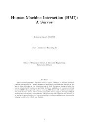
of a model’s equations). Figure 1 shows the space of possible models with a reference 

system defined by the three quantities mentioned above (the entities in this reference 

system will be described in the following paragraphs). 

The theory of schemata in genetic programming has had a difficult child- 

1 The only Markov chain model available for genetic programming and variable-length genetic algorithms 

to date is the one recently developed in (Poli et al., 2001), which, however, is only applicable to homologous 

crossover operators. We hope that by following a similar approach the theory developed in this paper will 

eventually make it possible to construct a usable Markov chain model of GP with subtree crossover. 

2 Evolutionary Computation Volume ?, Number ?

Coarse 

Graining of 

Right-hand 

Side 

Macroscopic 

Degree of 

Approximation 

Microscopic 

Exact Approximate 

Exact Schema Theorems 

for Schemata of Different Order 

Approximate Schema Theorems 

for Schemata of Different Order 

General Schema Theory for GP: Part II 

Microscopic Macroscopic 

Figure 1: Space of GA/GP schema-based models. 

Tracking Schema Behaviour by 

Summing over Properties of 

Each Member of the Population 

Coarse 

Graining of 

Left-hand 

Side 

hood. Some excellent early efforts led to different worst-case-scenario schema theorems 

(Koza, 1992; Altenberg, 1994; O’Reilly and Oppacher, 1995; Whigham, 1995; Poli 

and Langdon, 1997b; Rosca, 1997). In Figure 1, each of these is represented as a collection 

of small dashed circles. 2 Only very recently have the first exact schema theories 

become available (Poli, 2000b; Poli, 2000a; Poli, 2001a) which give exact formulations 

(rather than lower bounds) for the expected number of instances of a schema at the next 

generation. 3 These exact theories are applicable to GP with one-point crossover (Poli 

and Langdon, 1997a; Poli and Langdon, 1997b; Poli and Langdon, 1998). They occupy 

the horizontal plane in Figure 1 and so they have high predictive and explanatory 

powers. Since one-point crossover is not widely used, 4 however, this work has had a 

limited impact. The work in (Poli, 2000a; Poli, 2001a) has remained the only proposal 

of an exact macroscopic schema theory for GP with any GP crossover operator until the 

recent extension of that work to the class of homologous crossovers (Poli and McPhee, 

2001c) and the work described in this paper. As a result the space of models for GP 

with mainstream operators such as standard crossover has remained almost empty for 

many years. 

This paper helps fill this theoretical gap by presenting an exact general schema 

theory for genetic programming which is applicable to standard crossover as well as 

2 Starting from the back of the reference system, the circles represent schema equations for schemata of 

increasing order. Because in those equations the coarse graining (schema order) of the quantity on the l.h.s. 

is the same as that of the quantity on the r.h.s., the circles lie on a vertical plane which includes the origin and 

the vertical axis. 

3 To be precise, one of the models proposed in (Altenberg, 1994) is an exact model. However, as discussed 

in Section 2.1.1, this is a microscopic model of the propagation of program components (subtrees) in GP with 

standard crossover, rather than a theorem about schemata as sets. This model allows one to compute the 

exact proportion of subtrees of a given type in an infinite population in the next generation given information 

about the programs in the current generation. In Figure 1, Altenberg’s model is within the elongated ellipsoid 

at the back of the reference system. 

4 In fact, we are not yet aware of any public domain GP implementations offering one-point crossover as 

an option. 

Evolutionary Computation Volume ?, Number ? 3


many other crossover operators. 5 This is a result that has been sought for a long time 

in the GP community (see Section 2), since the development of a precise schema theory 

seemed the most natural way to give GP a theoretical foundation. Our theory 

includes two main results describing the propagation of GP schemata: a microscopic 

schema theorem and a macroscopic one. These models occupy the horizontal plane 

in Figure 1 and so they have high predictive and explanatory powers, like their predecessors 

for one-point crossover. The microscopic version is applicable to crossover 

operators which replace a subtree in one parent with a subtree from the other parent 

to produce the offspring. So the theorem covers standard GP crossover (Koza, 1992) 

with and without uniform selection of the crossover points, one-point crossover (Poli 

and Langdon, 1997b; Poli and Langdon, 1998), size-fair crossover (Langdon, 1999b; 

Langdon, 2000b), strongly-typed GP crossover (Montana, 1995), context-preserving 

crossover (D’haeseleer, 1994) and many others. In Figure 1, this model is within the 

elongated ellipsoid at the back of the reference system. The macroscopic version is valid 

for a large class of crossover operators in which the probability of selecting any two 

crossover points in the parents depends only on the parents’ size and shape. So, for example, 

it holds for all the above-mentioned crossover operators except strongly typed 

GP crossover. This model is represented by the elongated dotted ellipsoids within the 

triangular dashed spline in the lower part of Figure 1. Both theorems can be applied to 

model most GP systems used in practice. 

This document is the second part of a two-part paper, the first part of which, (Poli 

and McPhee, 2003), introduced the important notion of node reference systems, the 

related concepts of functions and probability distributions over such reference systems, 

and some probabilistic models of different crossover operators, all of which are used in 

Part II. So, the reader should be familiar (or at least should have available) Part I before 

delving into Part II. 

Part II is organised as follows. Firstly, we provide a review of earlier relevant work 

on schemata in Section 2. Then, we show how the machinery introduced in Part I can 

be used to derive a general microscopic schema theorem for GP with subtree-swapping 

crossover in Section 3. We transform this into a macroscopic schema theorem valid for 

a large set of commonly used subtree-swapping crossover operators in Section 4. In 

Section 5 we show how the theory can be specialised to obtain schema theorems for 

specific types of crossover operators, and how it can be used to obtain other general 

results, such as an exact definition of effective fitness and a size-evolution equation for 

GP with subtree-swapping crossover. In Section 6 we provide some examples which, 

together with the discussion on the practicality of the approach and the summary of 

some very recent applications of the theory provided in Section 7, further illustrate its 

explanatory and predictive powers. Some conclusions are drawn in Section 8. 

2 Background 

Schemata are sets of points in the search space sharing some feature. For example, in 

the context of GAs operating on binary strings, a schema (or similarity template) is 

syntactically a string of symbols from the alphabet ¡ 0,1,*¢ , like *10*1. The character * is 

interpreted as a “don’t care” symbol, so that, semantically, a schema represents a set of 

bit strings. For example the schema *10*1 represents a set of four strings: ¡ 01001, 01011, 

11001, 11011¢ . 

5 Early versions of some of this work were presented in (Poli, 2001b) and, to a lesser degree, (Poli and 

McPhee, 2001b). This paper is much more detailed, however, and includes a number of new results and 

examples. 



Typically schema theorems are descriptions of how the number (or the proportion) 

of members of the population belonging to a schema varies over time. As we noted 

in (Poli et al., 1998), for a given schema £ the selection/crossover/mutation process 

can be seen as a Bernoulli trial (a newly created individual either samples or does not 

sample £ ) and, therefore, the number of individuals sampling £ at the next generation, 

¤¦¥ £¨§�©�� , is a binomial stochastic variable. So, if we denote with � ¥ £�§�©�� the success 

probability of each trial (i.e. the probability that a newly created individual samples £ ), 

which we term the total transmission probability of £ , an exact schema theorem is simply 

� where is the population size and �� 

is the expectation operator. Holland’s and 

� 

other worst-case-scenario schema theories (Holland, 1975; Goldberg, 1989b; Whitley, 

1994) normally provide a lower bound � ¥ £¨§�©�� for or, equivalently, for �� £¨§�©�� . ¤�¥ 

One of the difficulties in obtaining schema theory results for GP is that the variable 

size tree structure in GP makes it more difficult to develop a definition of GP schema 

having the necessary power and flexibility. Several alternatives have been proposed in 

the literature, each of which define schemata as composed of one or multiple trees or 

fragments of trees. In some definitions (Koza, 1992; Altenberg, 1994; O’Reilly and Oppacher, 

1995; Whigham, 1995) schema components are non-rooted and a schema is seen 

as a set of subtrees that can be present multiple times within the same program. The 

focus in these theories is to predict how the number or the frequency of such subtrees 

varies over time. In more recent definitions (Poli and Langdon, 1997b; Rosca, 1997) 

schemata are represented by rooted trees or tree fragments. These definitions make 

schema theorem calculations easier and consequently form the basis of this work. 

In the next sub-sections, we will briefly summarise the main features of early GP 

schema theories, and then we will describe the definition introduced in (Poli and Langdon, 

1997b; Poli and Langdon, 1998) which is what is used in the rest of this paper and 

in a number of other recent theoretical developments (Poli, 2000a; Poli, 2000b; Poli and 

McPhee, 2001b; McPhee and Poli, 2001; Poli and McPhee, 2001a; McPhee et al., 2001; 

Poli and McPhee, 2001c; Poli et al., 2001). This will be followed by a description of 

the first two exact schema theorems for rooted GP schemata (Poli, 2000a; Poli, 2000b) 

which have inspired the work in this paper. Then we introduce the concept of effective 

fitness which is closely related to schema theories. We conclude this section with a brief 

discussion on the possible criticisms for schema theories. 

�� ¤¦¥ £�§�©�� ¥ £¨§�©��§ (1) 

2.1 Early Efforts in Developing a Schema Theory for GP 

Steps towards the development of a schema theory for genetic programming started 

as early as 1992. These early attempts concentrated on the propagation of program 

components (often seen as potential building blocks for GP) in the population. Starting 

in 1997, however, some researchers began treating schemata as sets of individuals, and 

focusing on understanding how the number of programs sampling a given schema 

(interpreted as a set) changes over time. (We use this latter approach in this paper.) 

2.1.1 Theories on Positionless Schema Component Propagation 

Koza (Koza, 1992, 116–119) made the first attempt to explain why GP works, producing 

an informal argument showing that Holland’s schema theorem (Holland, 1975) would 

work for GP as well. The argument was based on the idea of defining a schema as the 

subspace of all trees which contain a predefined set of subtrees. According to Koza’s 

definition a schema £ is represented as a set of S-expressions; for example the schema 



=¡ (+ 1 x), (* x y)¢ represents all programs including at least one occurrence 

£ 

of the expression (+ 1 x) and at least one occurrence of (* x y). Koza’s definition 

gives only the defining components of a schema not their position, so the same schema 

can be instantiated (matched) in different ways, and therefore multiple times, in the 

same program. 

Altenberg produced a probabilistic model of genetic programming which led to 

the first mathematical formulation of a schema theorem for GP (Altenberg, 1994). On 

the assumptions that the population is infinitely large, that there is no mutation, and 

that fitness proportionate selection is used, Altenberg obtained an equation which allows 

one to calculate the frequency of a given program in the next generation in terms 

of quantities such as: the fitness and frequency of the programs in the population, 

the average fitness of the programs in the population, the probability that inserting a 

given expression in a parent program will produce a given offspring program, and the 

probability that crossover will pick up a given expression (see (Altenberg, 1994) and 

also (Langdon and Poli, 2002) where a detailed example is provided). This model is 

important because it explicitly considers all ways in which programs can be created. It 

describes the propagation of programs under standard crossover assuming that only 

one offspring is produced as a result of each crossover operation. From this model, 

defining a schema as being a subexpression (or component), Altenberg obtained an expression 

for the average chance of finding a given expression in the population at the 

next generation as a function of a number of microscopic descriptors of the state of the 

current population. This expression can be considered an exact microscopic subtreeschema 

theorem for GP with standard crossover and infinite populations. Altenberg 

did not analyse its components in more detail, but he indicated that a simpler schema 

theorem could be obtained by neglecting the effects of crossover. (Note that Altenberg’s 

notion of schema is that a schema is a subexpression. This is not exactly the same as the 

notion introduced by Koza, where a schema could contain multiple subexpressions.) 

Koza’s notion of schema was formalised and extended by O’Reilly (O’Reilly and 

Oppacher, 1995) who derived a schema theorem for GP in the presence of fitnessproportionate 

selection and crossover. The theorem was based on the idea of defining 

a schema as an unordered collection (a multiset) of subtrees and tree fragments. Tree 

fragments are trees with at least one leaf that is a “don’t care” symbol (’#’) which can 

be matched by any subtree (including subtrees with only one node). For example the 

£ =¡ schema (+ # x), (* x y), (* y)¢ x represents all the programs including 

at least one occurrence of the tree fragment (+ # x) and at least two occurrences of 

(* x y). The tree fragment (+ # x) is present in all programs which include a + 

having x as the second argument. O’Reilly’s definition of schema allowed her to derive 

a worst-case-scenario schema theorem which provided a rather pessimistic lower 

bound for the expected number of instances of a given schema in the population at the 

next generation as a function of macroscopic quantities such as the mean fitness of the 

instances of the schema in the current generation. Like Koza’s definition, O’Reilly’s 

schema definition gives only the defining components of a schema and not their position, 

so the same schema can again be instantiated in different ways, and therefore 

multiple times, in the same program. As a result, her schema theorem describes the 

way in which the components of the representation of a schema propagate from one 

generation to the next, rather than how the number of programs sampling a given 

schema changes over time. 

In the framework of his GP system based on context free grammars (CFG-GP) 

Whigham produced a concept of schema for context-free grammars and a related 



schema theorem (Whigham, 1995; Whigham, 1996). In CFG-GP programs are generated 

by applying a set of rewrite rules taken from a pre-defined grammar to a start 

symbol S. In CFG-GP the individuals in the population are derivation trees whose internal 

nodes are rewrite rules and whose terminals are the functions and terminals used 

in the program. Whigham defines a schema as a partial derivation tree rooted in some 

non-terminal node, i.e. as a collection of rewrite rules organised into a single derivation 

tree. So, a schema represents all the programs that can be obtained by completing the 

schema and all the programs represented by schemata which contain it as a component. 

When the root node of a schema is not S, the schema can occur multiple times in the 

derivation tree of the same program because of the absence of positional information in 

the schema definition. Whigham’s definition of schema led him to derive an interesting 

worst-case-scenario schema theorem which provides a lower bound for the number of 

instances of a schema at the next generation as a function of some macroscopic quantities 

such as the probabilities of disruption of schemata under crossover and mutation, 

and the fitness of the schema. Like in Altenberg and O’Reilly’s cases, this theorem describes 

the way in which the components of the representation of a schema propagate 

from one generation to the next, rather than the way the number of programs sampling 

a given schema changes over time. 

2.1.2 Theories on Positioned Schema Propagation 

In 1997 two schema theories (developed at the same time and independently) were 

proposed (Rosca, 1997; Poli and Langdon, 1997b) in which schemata are represented 

using rooted trees or tree fragments. The rootedness of these schema representations 

is very important as they introduce in the schema definition the positional information 

lacking in previous definitions of schema for GP. As a consequence a schema can be 

instantiated at most once within a program and studying the propagation of the components 

of the schema in the population is equivalent to analysing the way the number 

of programs sampling the schema changes over time. 

Rosca (Rosca, 1997) proposed a definition of schema, called rooted tree-schema, in 

which a schema is a rooted contiguous tree fragment. For example, the rooted treeschema 

£ =(+ # x) represents all the programs whose root node is a + with x as 

its second argument. Rosca derived a microscopic schema theorem for GP with standard 

crossover (when crossover points are selected uniformly) which provided a lower 

bound for the expected number of individuals belonging to a schema in the next generation 

as a function of quantities such as the size of the programs matching the schema, 

their fitness and the order of a schema. 

In (Poli and Langdon, 1997b) we proposed a simple definition of rooted schema 

for GP which allowed us to derive a worst-case-scenario schema theorem for GP; this 

definition has subsequently been used to derive a variety of exact results, including 

those reported in this paper. The definition is as follows: 

Definition 1 (GP Schema) A GP schema is a tree composed of functions from the ��¡�� set 

and terminals from the set ��¡��¢ , where � and � are the function and terminal sets used 

¢ 

in a GP run. 6 The � primitive is a “don’t care” symbol which stands for a single terminal or 

function. The � ¥ £�� order of a GP £ schema is the number non-� of symbols it contains. 

A schema £ represents programs having the same shape as £ and the same la- 

6 In this paper we use the convention that the root node of a program or a schema also has an output link. 

As a result there is always a one-to-one correspondence between nodes and links, and, therefore, we can 

consider crossover points either as nodes or as links. We will also assume that the root node (or its output 

link) can be chosen for crossover. 



Fixed Size and 

Shape Schema 

+ 

x = 

y = 

+ 

x * 

Sample 

Programs 

y x 

x 

+ 

+ 

y x 

Figure 2: Fixed-size-and-shape GP schema and some of its instances. 

bels for the non-� nodes. For example, if � =¡ +, *¢ and � =¡ x, y¢ the schema 

(+ x (= y =)) represents the set containing the four programs (+ x (+ y x)), 

(+ x (+ y y)), (+ x (* y x)) and (+ x (* y y)) (see Figure 2). Note that in 

the other definitions of GP schema mentioned above, schemata divide the space of programs 

into subspaces containing programs of different sizes and shapes. Our schemata, 

on the other hand, partition the program space into subspaces of programs of fixed size 

and shape, and we will therefore refer to them as fixed-size-and-shape schemata. 

In order to derive a GP schema theorem for fixed-size-and-shape schemata in (Poli 

and Langdon, 1997b; Poli and Langdon, 1998) we used non-standard forms of mutation 

and crossover, namely point mutation and one-point crossover. Point mutation is the 

substitution of a node in the tree with another node with the same arity. One-point 

crossover works by selecting a single shared crossover point in the two parent programs 

and then swapping the corresponding subtrees, like standard crossover. To account for 

the possible structural diversity of the two parents, one-point crossover analyses the 

two trees starting from the root nodes and limits the selection of the crossover point 

to the parts of the two trees which have the same topology. 7 The resulting schema 

theorem (see (Poli and Langdon, 1997b; Poli and Langdon, 1998)) is a generalisation of 

a version of Holland’s schema theorem (Whitley, 1994) for variable size structures (as 

discussed in (Poli, 2001a)). Like Holland’s theorem it is a worst-case-scenario model, 

i.e., it provides only a lower bound for � ¥ £¨§�©�� . 

2.2 Exact GP Schema Theory for One-point Crossover 

In (Poli, 2000b; Poli, 2000a) we were able to improve our worst-case-scenario schema 

theorem producing an exact schema theory for GP with one-point crossover, thanks to 

the introduction of a generalisation of the definition of GP schema: the hyperschema. 

Definition 2 (Hyperschema) A GP hyperschema is a rooted tree composed of internal 

nodes from the set ��¡��¢ and leaves from ��¡��§��¢ . The operator = is, as before, a 

“don’t care” symbol which stands for exactly one node, while the operator # stands for any valid 

subtree. 

For example, the hyperschema (* # (= x =)) represents the set of all programs 

with the following characteristics: a) the root node is a product, b) the first argument 

of the root node is any valid subtree, c) the second argument of the root node is any 

function of arity two, d) the first argument of this function is the variable x, e) the 

second argument of the function is any valid node in the terminal set. 

7 This is called the common region, and has been defined formally in Part I (Poli and McPhee, 2003). 



Using hyperschemata, it is possible to obtain the following exact microscopic expression 

for the total transmission probability for a fixed-size-and-shape GP schema £ 

under one-point crossover: 8 

where 

and 

� 

� 

� 

� 

�� 

� 

� 

� 

� 

� 

� xo ¥ £�§�©�� 

¥ £¨§�©�� ¥ �� ¥ £¨§�©��¨�� xo 

¥ £¨§�©�� (2) 

� 

¥�� §�©�� ¥�� §�©�� 

�� 

� 

� § � � � ¥�� 

� �� is the crossover probability; 

¥ £¨§�©�� is the selection probability of the schema £ ; � 9 

¥�� §�©�� is the probability of selecting program � � ; 10 

� � �� ¥��¥ £¨§�� ¥��¨��¥ £¨§�� (3) 

�� 

the first two summations are over all the individuals in the population; 

§ �� is the set of indices of the crossover points in the common region between 

¥�� 

program � � and program � � (see Part I); 

�� ¥�� § �� is the number of nodes in the common region; 

� ¥�� is a function which returns 1 if � is true, 0 otherwise; 

��¥ £¨§�� is the hyperschema obtained by replacing all the nodes in £ on the path 

between crossover point � and the root node with = nodes, and all the subtrees 

connected to those nodes with # nodes (illustrations of this and the following hyperschema 

are given below); 

£¨§�� is the hyperschema obtained by replacing the subtree of £ below crossover 

��¥ 

� point with a # node; 

if a crossover point � is in the common region between two programs but it is 

outside the schema £ , then ��¥ £¨§�� and ��¥ £¨§�� are empty sets. 

The hyperschemata ��¥ £¨§�� and ��¥ £¨§�� are important because, if one crosses over 

any individual in ��¥ £¨§�� at point � with any individual in ��¥ £¨§�� , the resulting offspring 

is always an instance of £ . 11 The converse is also true: if an individual which 

has been created by crossover belongs to a schema £ then there exists at least one � 

such that the parents of the individual belong to ��¥ £¨§�� and ��¥ £�§�� . (One can easily 

verify this by noting that if this was not true, then the theorem which led to Equations 2 

and 3 could not be true.) 

8Equations 2 and 3 are in a slightly different form than the result in (Poli, 2000b). However, the two results 

are equivalent ��¨�� since �� and . 

9In fitness proportionate selection this is given �� 

by , �� where is the number 

�� 

of programs matching the schema � at generation � , �� is the mean fitness of such programs, � 

�� 

mean fitness of the programs in the population, � and is the population size. 

10In fitness selection�� 

proportionate 

�� 

�� 

where �� is the fitness of program � . 

11 The symbol � stands for “lower part of”, while � stands for “upper part of”. 

�� is the 



0 

H L(H,1) 

* 

1 2 

= + 

3 4 

x = 

* 

= + 

= 

x = 

= + 

= 

x = 

= # 

U(H,1) 

* 

= + 

* 

x = 

# + 

x = 

L(H,3) 

* 

= + 

= 

x = 

= = 

= 

x = 

# = 

x # 

U(H,3) 

* 

= + 

* 

x = 

= + 

# = 

Figure 3: Example of schema and some of its potential hyperschema building blocks. 

The crossover points in £ are numbered as shown in the top left. 

Let us consider an example which shows how ��¥ £¨§�� and ��¥ £¨§�� are built. If 

(* = (+ x =)) then, as indicated in the second column of Figure 3, £�� ¥ £¨§�� 

is obtained by first replacing the root node with a = symbol and then replacing the 

right subtree of the root node with a # symbol, obtaining (= = #). The schema 

£¨§�� is obtained by instead replacing the subtree below the crossover point with 

��¥ 

a # symbol obtaining (* # (+ x =)), as illustrated in the third column of Figure 3. 

The fourth and fifth columns of Figure 3 show how ��¥ (= # (= x #)) and 

£¨§�� 

£¨§�� (* = (+ # =)) are obtained. 

��¥ 

In (Poli, 2000a) we transformed Equations 2 and 3 into a macroscopic model in 

which12 � xo ¥ £¨§�©�� 

�� 

� � 

§ � ¥�� 

� 

� 

� 

�� 

� � � ¥��¥ £¨§�� 

�� 

� 

§�©�� ¥��¥ £¨§�� 

� 

§�©��§ (4) 

where the first two summations are over all the possible program shapes �� , �� , �� , 

i.e. all the possible fixed-size-and-shape schemata containing = signs only. The sets 

£¨§�� 

� 

and ��¥ £¨§�� 

� 

are either empty or are (or can be represented by) fixed- 

��¥ 

size-and-shape schemata. So, the result expresses the total transmission probability of 

12 Equation 4 is in a slightly different form than the result in (Poli, 2000a). However, the two results are 

equivalent since ��¨�� and �� . 



only using the selection probabilities of a set of lower- (or same-) order schemata. 

£ 

Section 6.1 gives an example of schema equation for one-point crossover for a population 

of variable length linear structures. 

As discussed in (Poli, 2001a), it is possible to show that, in the absence of mutation, 

Equation 4 generalises and refines not only the GP schema theorem in (Poli and 

Langdon, 1997b; Poli and Langdon, 1998) but also a version of Holland’s (Holland, 

1975; Whitley, 1994) and more modern GA schema theory (Stephens and Waelbroeck, 

1997; Stephens and Waelbroeck, 1999). For a more detailed treatment and a variety of 

examples and comparisons see (Langdon and Poli, 2002, Chapter 5). 

2.3 Effective Fitness 

The idea of effective fitness is associated with the observation that two individuals with 

the same fitness may in fact have very different characteristics in terms of their ability 

to transmit their genetic material to future generations. For example, it is possible that 

the offspring of the first individual produced via crossover and/or mutation tend to be 

fit, while those of the second individual tend not to be so. So, while the former will be 

selected and used for reproduction, the latter will not. As a result, it is as if the first 

individual we considered had a higher effective fitness than the second, although they 

have the same actual fitness. 

Their concept of effective fitness was introduced in GP by Nordin and Banzhaf 

in (Nordin and Banzhaf, 1995; Nordin et al., 1995) to explain the reasons for bloat 

and active-code compression. Fundamentally the idea was to interpret the effects of 

crossover in a GP system by imagining an equivalent GP system in which selection 

only is used, but in which each individual was given an appropriate effective fitness 

(which takes the reproductive success of the individual into account) rather than the 

original fitness. The concept of effective fitness is very similar to the concept of operatoradjusted 

fitness (not to be confused with Koza’s adjusted fitness (Koza, 1992)) introduced 

for GAs a few years earlier by Goldberg in (Goldberg, 1989a, page 155). Nordin and 

Banzhaf’s notion of effective fitness and Goldberg’s notion of operator-adjusted fitness 

are essentially the same, although their mathematical definitions are applicable to different 

representations and operators. Unfortunately, these mathematical definitions 

were based on approximate models of GP and GAs (which neglected the constructive 

effects of the genetic operators), and, therefore, they were unable to fully capture the 

original idea of effective fitness. 

Stephens and Waelbroeck (Stephens and Waelbroeck, 1997; Stephens and Waelbroeck, 

1999) succeeded in this, when they independently rediscovered the notion of 

effective fitness. Their effective fitness of a schema is implicitly defined through the equation 

¤�¥ ¤¦¥ 

¥ 

£¨§�©�� 

£¨§�©�� 

�� 

©�� 

§ 

£¨§�©�� ¥ 

assuming that fitness proportionate selection is used. Noting that �� 

� 

� 

�� 

� � 

� �� 

� 

¥ and � £¨§�©�� 

� � �� 

�� 

� �� 

� �� , we can obtain an explicit form 

�� 

¥ £�§�©�� 

¥ £¨§�©�� 

¥ £¨§�©�� 

� 

� 

¥ £¨§�©��§ (5) 

using � ¥ £¨§�©�� from (Stephens and Waelbroeck, 1997; Stephens and Waelbroeck, 1999). 

Using the exact schema result reported in the previous section (Equations 2 and 4), 

in (Poli, 2000a) we extended the exact notion of effective fitness provided in (Stephens 



and Waelbroeck, 1997; Stephens and Waelbroeck, 1999) to GP with one-point crossover, 

obtaining 

� �� 

¥ £¨§�©�� 

� 

¥ £¨§�©�� 

� 

� � � � 

�� 

� �� 

� � 

� � 

¥��¥ £¨§�� 

� 

§�©�� ¥��¥ £¨§�� 

�� 

� � 

§ � 

� 

¥�� 

(see (Poli, 2000a; Poli, 2001a) for more details). This result gives the exact effective fitness 

for a GP schema under one-point crossover: it is not an approximation or a lower bound. 

2.4 Criticisms to Schema Theories 

� 

§�©�� 

�� ¥ £¨§�©�� 

In the past the usefulness of schemata and the schema theorem has been widely criticised 

(see for example (Chung and Perez, 1994; Altenberg, 1995; Fogel and Ghozeil, 

1997; Fogel and Ghozeil, 1998)). While some criticisms are really not justified (as discussed 

in (Radcliffe, 1997; Poli, 2000d)) others are reasonable, although they apply 

mainly to the old, worst-case-scenario-type schema theories. 

Perhaps the most important criticism of this kind is that worst-case-scenario 

schema theorems only give lower bounds on the expected value of the number of individuals 

sampling a given schema at the next generation, and cannot be used to make 

predictions over multiple generations. Clearly, there is some truth in this. For these 

reasons it has been frequently suggested that schema theorems are nothing more than 

trivial tautologies of no use whatsoever. However, this position regarding schema theorems 

is not justified anymore. Indeed, modern schema theorems, such as the ones presented 

in this paper, provide exact values rather than lower bounds (e.g. see (Stephens 

and Waelbroeck, 1997; Stephens and Waelbroeck, 1999)). 

Clearly, exact schema theorems still suffer from the problem that the quantity on 

the left-hand-side includes an expectation operator. However, this is not a fault in the 

approach: it is simply due to the stochastic nature of evolutionary algorithms. The expectation 

operator can be removed as indicated in (Poli, 1999; Poli, 2000c) by converting 

an exact statement on the expectation into a probabilistic statement over the confidence 

interval of the predicted quantity. As shown in (Poli et al., 2001), once an exact schema 

theorem is available, it is also possible to use it to model and study an evolutionary 

algorithm using Markov chain theory. In (Poli et al., 2001) we did this for GP with 

homologous crossover by extending Vose’s model for fixed length GAs (Nix and Vose, 

1992; Vose, 1999) and using the exact schema equations to calculate the chain’s transition 

matrix. In turn, the availability of Markov chain model allows the calculation 

of the probability distribution over the space of all possible populations at any time in 

the future. So, schema equations can be used to make long term predictions. However, 

whatever the adopted model, we cannot change the fact that we are dealing with 

processes in which randomness is present in a variety of places, and which, therefore, 

do not allow exact predictions over multiple generations (Poli, 2000c). The only exception 

to this is when the population is infinite. In this case the expectation operator 

can be removed from schema theorems, making the analysis considerably easier. For 

example, the schema equations can be integrated to obtain the system’s trajectory for 

any number of generations. (We will use this approach in the examples of Section 6.2.) 

This infinite-propulation trajectory can be considered as a reasonable approximation 

for what happens in finite populations, provided it does not span too many generations 

and the population is sufficiently large. 

12 Evolutionary Computation Volume ?, Number ? 

�

VA Hyperschema Sample Instances 

# 

x + 

= # 

+ 

x + 

2 x 

* 

x + 


x + 

2 x 

IF 

x + 

2 x 

Figure 4: Example of variable-arity hyperschema and some of its instances. 

3 Microscopic Exact GP Schema Theorem for Subtree-swapping 

Crossovers 

* 

x + 

For simplicity in this and the following sections we will use a single index to identify 

nodes in a node reference system unless otherwise stated. We can do this because, as 

indicated in Part I (Poli and McPhee, 2003), there is a one-to-one mapping between 

pairs of coordinates and natural numbers. 

In order to obtain a schema theory valid for subtree-swapping crossovers, we need 

to extend the notion of hyperschema summarised in Section 2.2. We will call this new 

form of hyperschema a Variable Arity Hyperschema or VA hyperschema for brevity. 

Definition 3 (VA Hyperschema) A Variable Arity hyperschema is a rooted tree composed 

of internal nodes from the set ��¨¡��§��¢ and leaves from ��¨¡��§��¢ , where � and � are the 

function and terminal sets. The operator = is a “don’t care” symbol which stands for exactly 

one node, the terminal # stands for any valid subtree, while the function # stands for exactly 

one function of arity not smaller than the number of subtrees connected to it. 

For example, the VA hyperschema (# x (+ = #)) (see Figure 4) represents all the 

programs with the following characteristics: a) the root node is any function in the 

function set with arity 2 or higher, b) the first argument of the root node is the variable 

x, c) the second argument of the root node is +, d) the first argument of the + is any 

terminal, e) the second argument of the + is any valid subtree. If the root node is 

matched by a function of arity greater than 2, the third, fourth, etc. arguments of such 

a function are left unspecified, i.e. they can be any valid subtree. 

VA hyperschemata generalise all previous definitions of rooted schemata in GP. 

For example, they generalise hyperschemata (Poli, 2000b; Poli, 2000a) (which are VA 

hyperschemata without internal # symbols). These in turn generalise the notion of 

fixed-size-and-shape schemata (Poli and Langdon, 1997b; Poli and Langdon, 1998) 

(which are hyperschemata without # symbols) and Rosca’s schemata (Rosca, 1997) 

(which are hyperschemata without = symbols). 

VA hyperschemata are useful because they can express the syntactic features the 

parents need to posses in order for them to produce instances of a specific schema 

of interest for any given pair of crossover points. Figure 5 illustrates how instances 

of the schema (* = (+ x =)) can be created for two different choices of crossover 

points. For example, if the root donating parent matches the VA hyperschema (* # 

(+ x =)) and the crossover point in it is the first argument of the root node, while 

the subtree donating parent matches the VA hyperschema (# # =) and the crossover 



VA Hyperschema 

Containing the 

Subtree-donating 

Parent 

# 

# = 

X 

Crossover 

Points 



Root-donating 

Parent 

* 

# + 

x = 

Fixed-size-and-Shape 

Schema 

* 

= + 

x = 



Subtree-donating 

Parent 

# 

# # 

X 



Root-donating 

Parent 

+ 

x = 

* 

= # 

Crossover 

Points 

Figure 5: Two different ways in which instances of the fixed-size-and-shape schema (* 

= (+ x =)) can be created. 

point in it is the second argument of the root node, then the offspring will necessarily 

match the fixed-size-and-shape schema (* = (+ x =)). 

Thanks to VA hyperschemata and to the models of crossover developed in Part 

I (Poli and McPhee, 2003), it is possible to obtain the following general result: 

Theorem 1 (Microscopic Exact GP Schema Theorem) The total transmission probability 

for a fixed-size-and-shape GP schema £ under a subtree-swapping crossover operator and no 

mutation is given by Equation 2 with 

xo � ¥ �� ¥�� §�©�� ¥�� §�©�� 

�� 

£�§�©�� 

where: 

� 

� 

� 

� 

� 

� 

� 

� 

¥ ��§�� § �� ¥��¥ £¨§�� ¥��¨��¥ £¨§��§�� 

�� 

(6) 

the first two summations are over all the individuals in the population; 

¥�� §�©�� and � ¥�� §�©�� are the selection probabilities of parents � �� and �� , respectively; 

the third summation is over all the crossover points (nodes) in the £ schema ; 

the fourth summation is over all the crossover points in the node reference system; 

¥ ��§�� § �� is the probability of selecting crossover point � in parent � �� and crossover 

� point in parent �� (see Part I); 

��¥ £¨§��§�� is the VA hyperschema obtained by rooting at coordinate � in an empty reference 

system the subschema of £ below crossover point � , then by labelling all the nodes on the 

path between node � and the root node with # function nodes, and finally labelling the 

arguments of those nodes which are to the left of such a path with # terminal nodes (an 

illustration of this hyperschema is given below); 

£¨§�� is the hyperschema obtained by replacing the subtree below crossover point � with 

��¥ 

a # node; 

if crossover point � is outside the schema £ , then ��¥ £¨§��§�� and ��¥ £�§�� are empty sets. 



The meaning of the hyperschema ��¥ £¨§�� is essentially the same as in Section 2.2 

(only the numbering for crossover points adopted there was different). The VA hyperschema 

��¥ £¨§��§�� represents the set of all programs whose subtree rooted at crossover 

point � matches the subtree of £ rooted in node � . The idea behind its definition is 

that, if one crosses over at point � any individual matching ��¥ £�§��§�� and at point � any 

individual matching ��¥ £¨§�� , the resulting offspring is always an instance of £ . 

Before we proceed with the proof of the theorem, let us look at one example of how 

��¥ £¨§��§�� is built (refer to Section 2 and Figure 3 to see how ��¥ £¨§�� is built). Let us consider 

the schema £�� (* = (+ x =)) and a node reference system with �� . As 

indicated in Figure 6, ��¥ £¨§ ¥ ��§��§ ¥ ��§�� is obtained through the following steps. Firstly, 

we root the subschema below crossover point ¥ ��§�� , i.e. the tree (+ x =), at coordinates 

¥ ��§�� in an empty reference system. Note that this is not just a rigid translation: 

while the + is translated to position ¥ ��§�� , its arguments need to be translated more, i.e. 

to positions ¥ ��§�� and ¥ ��§�� , because of the nature of the reference system used. Then, 

we label the nodes at coordinates ¥�� § � � and ¥ ��§�� with # functions since these are on 

the path between node ¥ ��§�� and the root. Finally, we label node (1,0) with a # terminal 

as it is the only argument of a node replaced with # to be to the left of the path between 

¥ ��§�� and the root node. 13 

Once the concept of ��¥ £�§��§�� is available, the theorem can easily be proven. 

Proof: Let � ¥�� § � � §��§��§�©�� be the probability that, at generation © , the selection/crossover 

process will choose parents � � and � � and crossover points � and � . 

Then, let us consider the function 

��¥�� § �� §��§��§�£�� ¥��¥ £¨§�� ¥��¨��¥ £¨§��§�� 

Given two parent programs, � � and � � , and a schema of interest £ , this function returns 

the value 1 if crossing over � � at position � and � � at position � yields an offspring 

in £ . It returns 0 otherwise. This function can be considered as a measurement 

function (see (Altenberg, 1995)) that we want to apply to the probability distribution 

� ¥�� § �� §��§��§�©�� of parents and crossover points at time © . Since �� , �� , � and � 

are stochastic variables with joint probability distribution � ¥�� § �� §��§��§�©�� , the function 

��¥�� § �� §��§��§�£�� can be used to define a stochastic variable �� ¥�� § �� §��§��§�£�� whose 

expected value is: 

�� 

�� 

� 

� � ��¥�� § � � §��§��§�£�� ¥�� § � � §��§��§�©�� (7) 

� Since is a binary stochastic variable, its expected value also represents the probability 

of it taking the value 1, which corresponds to the probability that the offspring of 

and �� be £ in , i.e. �� ¥ £¨§�©�� . �� 

We can write 

¥�� § �� §��§��§�©��¦� ¥ ��§�� § �� ¥�� §�©�� ¥�� §�©��§ (8) 

� 

13One might think �� that is a generalisation of the �� hyperschema defined in Section 2. In 

�� fact, is very similar �� to . However, there are differences between these two hyperschemata. 

�� In the nodes on the path to the root node � in are replaced with = symbols. Each of these stands for a 

function of a fixed arity, which one can determine from the structure � of . �� In the nodes in the path 

�� to are filled with # symbols. Each of these stands for a function of arity not smaller than a value which 

can be determined from the particular column occupied by the node (but obviously not bigger �� than ). 

We will further discuss the relation between the VA �� hyperschema and the �� hyperschema at 

the end of Section 5.3. 

Evolutionary Computation Volume ?, Number ? 15 

� �


0 

1 

2 

Layer 

d 

0 

1 

2 

Layer 

d 

3 

0 

1 

2 

Layer 

d 

3 

* 

= 

+ 

L(H,(1,1),(2,2)) 

0 1 2 3 

x = 

0 1 2 3 

0 1 2 3 

# 

# 

# 

+ 

+ 

Column 

i 

Column 

4 5 i 

x = 

Column 

4 5 i 

x = 

Figure 6: Phases in the constructions of the VA hyperschema building block 

��¥ £¨§ ¥ ��§��§ ¥ ��§��§�� of the schema £�� (* = (+ x =)) within a node coordinate sys- 

tem with �� . 



where � ¥ ��§�� § �� is the conditional probability that crossover points � and � will be 

selected when the parents are �� and �� , while � ¥�� §�©�� and � ¥�� §�©�� are the selection 

probabilities for the parents. Substituting Equation 8 into Equation 7 and remembering 

that if crossover point � is outside the schema £ , then ��¥ £¨§��§�� and ��¥ £¨§�� are empty 

sets, yields 

�� ¥�� §�©�� ¥�� §�©�� 

�� 

�� 

4 Macroscopic Exact GP Schema Theorem 

�� ¥�� § �� §��§��§�£�� ¥ ��§�� § �� (9) 

� 

In order to transform Equation 6 into an exact macroscopic description of schema propagation 

we will need to make one additional assumption on the nature of the subtreeswapping 

crossovers used: that the choice of the crossover points in any two parents, 

�� and �� , depends only on their shapes, ��¥�� and ��¥�� , not on the actual labels 

of their nodes, i.e. that � ¥ ��§�� § �� ¥ ��§�� ¥�� § ��¥�� . We will term such operators 

node-invariant crossovers. Most GP crossover operators used in practice fall in this 

category. 

Theorem 2 (Macroscopic Exact GP Schema Theorem) The total transmission probability 

for a fixed-size-and-shape GP schema £ under a node-invariant subtree-swapping crossover 

operator and no mutation is given by Equation 2 with 

xo 

¥ £¨§�©�� 

�� 

�� ¥ ��§�� § � 

� 

�� ¥��¥ £¨§�� §�©�� ¥��¥ £¨§��§�� §�©��§ (10) 

� 

where the schemata �� , �� , �� are all the possible fixed-size-and-shape schemata of order 0 

(program shapes) and the other symbols have the same meaning as in Theorem 1. 

� 

Proof: The schemata � � � �� , , represent disjoint sets of programs and their 

union represents the whole search space. As a result, for every � , there is exactly 

� one such � ¥�� 

� 

�� that , which allows us to rewrite any expression � � � � � as 

� ¥��¦� 

� 

� � ¥��¦� 

� 

� �� 

� ¥ ��§�� § �� ¥�� 

� 

� . If we set � �� ¥�� §�©�� ¥�� §�©�� 

£¨§�� ¥��¥ £�§��§�� , we can then rewrite Equation 6 as: 

��¥ 

xo 

¥ £�§�©�� (11) 

� 

� � �� 

� � �� ¥�� 

� 

� � � � � � �� ¥�� 

� 

� � 

�� 

� 

� 

� � ¥�� 

� � ¥�� 

� 

� � 

� 

¥�� §�©�� ¥�� §�©�� 

�� ¥ ��§�� § �� ¥��¥ £¨§�� ¥��¥ £¨§��§�� 

� � � 

�� 

� � �� 

�� 

� ¥�� §�©�� ¥�� §�©�� 

�� 

� � � ¥ ��§�� § � � � � ¥�� ¥ £�§�� ¥�� ¥ £¨§��§�� 

� 

� � 

� 

� ¥ ��§�� § �� ¥ ��§�� ¥�� § ��¥�� For node-invariant crossover operators , which substituted 

into the previous equation gives: 

� � � �� 

�� 

�� 

�� 

� �� 

¥�� §�©�� ¥�� §�©�� 

�� 

� 

� 

�� ¥ ��§�� ¥�� § ��¥�� ¥�� ¥ £¨§�� ¥�� ¨��¥ £¨§��§�� 


�


�� 

�� 

� � �� 

�� 

�� 

�� 

� 

�� ¥ ��§�� 

¥�� §�©�� ¥�� §�©�� 

�� 

� 

� � 

§ � 

�� ¥ ��§�� 

�� 

� 

� � 

� 

� 

��¥ £�§��§�� 

and 

� 

§ � 

� 

� ¥�� ¥ £¨§�� ¥�� ¥ £�§��§�� 

� 

� 

�� 

� � � � £¨§�� 

� ¥�� ¥�� §�©�� ¥�� ¥ 

�� 

§�©�� 

� 

� ¥�� ¥ £¨§��§�� 

� 

�� 

� �� 

If non-empty, the sets ��¥ � 

� 

are (or can be represented 

£¨§�� 

by) fixed-size-and-shape schemata. So, the theorem expresses the total transmission 

probability £ of only using the selection probabilities of a set of lower- (or same-) order 

schemata. 

5 Applications and Specialisations 

In this section we show how the theory can be specialised to obtain schema theorems 

for specific crossover operators, and we illustrate how it can be used to obtain other 

general theoretical results, such as an exact definition of effective fitness and a sizeevolution 

equation for GP with subtree-swapping crossover. 

5.1 Macroscopic Exact Schema Theorem for GP with Standard Crossover 

Let us specialise Theorem 2 to standard crossover (Koza, 1992). For simplicity we will 

do this for the case in which the crossover points are selected uniformly at random. 

In order to use the theorem we need to check whether standard crossover is 

node invariant, i.e. whether it is true � ¥ ��§�� § �� ¥ ��§�� ¥�� § ��¥�� that . The 

notion of name function introduced in Part I is applicable to any tree, including 

schemata. If � is an order-0 schema (i.e. a program � ¥�� §��§ � �� shape) exactly when 

§�� is in the schema. It then follows that if ¥�� is a program and ��¥�� is its shape, � 

¥�� §��§ � �� if and only if � ¥�� §��§ ��¥�� . Also, clearly � ¥�� ¥��¥�� . So, using 

� 

and � to represent the coordinates � ¥�� and §�� ¥�� , respectively, the expression of 

§�� 

� ¥�� §�� § �� §�� § �� in Part I can be transformed as follows 

�� 

� �� ¥ ��§�� § � � �� 

So, we can replace � ¥ ��§�� 

� 

§ � 

� 

¥ � ¥ ��§ �� ¥ � ¥ ��§ �� 

� 

¥�� ¥�� 

� ¥��¥�� ¥��¥�� 

� 

�� ¥ ��§�� ¥�� § ��¥�� 

� 

� 

�� 

¥ � ¥ ��§ ��¥�� ¥ � ¥ ��§ ��¥�� 

� 

� in Equation 10 with the expression 

� ¥ � ¥ ��§ � 

obtaining, after appropriate simplification: 

� 

�� ¥ � ¥ ��§ � �� 

¥�� 

� 

�� ¥�� 

� 

� � 

� 

�� 

Theorem 3 (Macroscopic Exact GP Schema Theorem for Standard Crossover) The total 

transmission probability for a fixed-size-and-shape GP schema £ under standard crossover 

with uniform selection of crossover points is given by Equation 2 with 

� xo ¥ £¨§�©�� 

� ¥�� 

� � 

¥�� 

� 

� �� 

�� 

� 

� 

� � 

� 

�� 

� ¥��¥ £¨§�� 

� 

§ 

§�©�� ¥��¥ £¨§��§�� 

� 

� 

� � 

§�©�� (12) 


�


5.2 Exact Schema Theorem for GP with Standard Crossover Acting on Linear 

Structures 

As an example let us further specialise the result in the previous section to the case of 

linear structures. In the case of function sets including only unary functions, programs 

and schemata can be represented as linear sequences of symbols like �� (see also 

Section 6.1), and so: 

� 

� 

� 

� 

The hyperschema ��¥�� §�� . 

The VA hyperschema ��¥�� 

§��§�� ¥ �� 

� 

� � �� , where the notation 

�� 

means �� ¥�� repeated times. This is equivalent to the non-VA hyperschema 

� 

� 

� 

� 

� � �� since, in the case of linear structures, � ’s in function nodes can be 

¥ �� 

� replaced by ’s. 

The set ��¥�� §�� 

The set ��¥�� §��§�� 

� 

�� 

� 

�� for , 

otherwise. 

� 

�� 

� �� ¥ � 

�� 

� 

� 

� 

� � �� if �� , 

�� ¥ 

� 

� otherwise. 

� 

By substituting these quantities into Equation 12 and performing some simplifications 

one obtains the following result 

� xo ¥�� §�©�� 

� 

� 

�� 

�¡ £¢ 

� 

� � � � 

� �� 

� � ¥ � 

�� §�©�� ¥�� 

� 

�� 

� 

� � �� §�©�� ¥�¥ � 

�� 

� (13) 

Equation 13 can be shown to be equivalent to the schema theorem for linear structures 

reported in (Poli and McPhee, 2001b). 

5.3 A Different Form of Macroscopic Schema Theorem for One-point Crossover 

As an additional example, we will derive a GP schema theorem for one-point crossover 

equivalent to the one described in Section 2.2. 

Again, in order to use Theorem 2 we need to first check whether one- 

point crossover is node invariant, i.e. whether it � ¥ ��§�� § �� 

is true that 

��¥�� § ��¥�� . It is easy to see that � ¥ ��§�� 

�� ¥��¥�� § ��¥�� , and that 

¥�� 

� 

§ �� 

§ �� if and only if � � ¥��¥�� § ��¥�� . Therefore, the expression of 

� � ¥�� 

¥�� §�� § �� §�� § �� in Part I can be transformed as follows � 

� �¥¤ � 

� �¦¤ � ¥ ��§�� § � � �� 

So, we can replace � ¥ ��§�� 

�� § �� if �� and � � 

§ ¥�� 

� otherwise, 

§ 

� 

�� ¥��¥�� § ��¥�� if �� and � � 

� � 

otherwise, 

� 

� �¥¤ � ¥ ��§�� ¥�� § ��¥�� 

� 

� 

§ � 

� 

¥�� § �� , 

� in Equation 10 with the expression 

� ¥ � � 

obtaining, after some simplification: 

� 

� 

§ � 

� 

�� ¥ �� ¥�� 

¥�� 

� 

§ � 

� § 

�� 

� 

� 

¥��¥�� § ��¥�� , 



Theorem 4 (Macroscopic Exact GP Schema Theorem for One-point Crossover) The 

total transmission probability for a fixed-size-and-shape GP schema £ under one-point 

crossover is given by Equation 2 with 

� xo ¥ £¨§�©�� 

�� 

� � 

§ � ¥�� 

� 

� 

�� 

� � 

�� 

� � � ¥��¥ £¨§�� 

�� 

� 

§�©�� ¥��¥ £¨§��§�� 

� 

§�©�� (14) 

This result is equivalent to Equation 4. To see this we need to show that summing over 

� 

� £�� ¥�� 

� 

§ � 

� 

� is the same as summing over � � ¥�� 

� 

§ � 

� � 

§�©�� ¥��¥ £¨§��§�� 

� 

§�©�� ¥��¥ £¨§�� 

� 

§�©�� ¥��¥ £¨§�� 

� 

� 

� 

� 

and that � ¥��¥ £¨§�� 

� 

�� £ , then the fact that if ��¥ � 

� � 

� 

£¨§�� ¥ � � � � £¨§�� 

¥�� 

� 

� � § �� £ The second follows from the 

. So, all the terms in 

Equation 4 for which but are zero. 

fact that ��¥ £¨§��§�� and ��¥ £ £¨§�� have exactly the same subtree of at exactly the same 

§�©�� . The first follows from 

position, while all their remaining nodes are “don’t care” symbols (of different kinds). 

So, either ��¥ � 

£¨§�� ¥ £¨§��§�� 

� 

� 

� and are both empty sets, or they are the same 

. 

fixed-size-and-shape schema. In either case ��¥ £�§�� 

5.4 Size-evolution Equation for GP with Subtree-swapping Crossover 

� 

� ��¥ £¨§��§�� 

Let us call any crossover operator for which � ¥ ��§�� § � � �� ¥ ��§�� § � � � a symmetric 

crossover operator. 

Theorem 5 (GP Average Size Evolution Equation) Let ¨ be the mean size of the programs 

in a GP population. Then, the expected value ¨ of at ©�� generation , �� ¥ ©�� , in a GP 

¨ 

system with a symmetric subtree-swapping crossover operator in the absence of mutation can 

equivalently be expressed in microscopic form as 

¨ ¥ ©�� 

�� 

��© 

where � denotes the population, or in macroscopic form as 

� ¥�� ¥�� §�©��§ (15) 

¨ ¥ ©�� ¥�� 

� 

�� ¥�� §�©�� (16) 

�� 

Proof: By definition the expected mean size of the individuals in a population at the 

next generation is given by 

¨ ¥ ©�� 

�� 

�� 

� ¥�� ¥�� §�©��§ 

where the summation is over all possible computer programs in the search space � . By 

substituting Equations 2 and 6 (specialised for £�� ) into this equation, one obtains 14 

¨ ¥ ©�� ¥ �� 

�� 

�� 

� � 

� 

¥�� ¤�¥�� §�©�� ¥�� §�©�� 

� 

� 

�� 

¥�� 

��© 

� 

� � � ¥ ��§�� § � � � � ¥�� ¨��¥�� §�� ¥�� ¨��¥�� §��§��§ 

� � 

��© 

� 

� ¥�� §�©�� ¥�� §�©�� 

where we did not � limit to range only over the crossover points in � because � if 

is outside � , then ��¥�� and §��§�� ¥�� are empty sets and so � ¥�� ¥�� §�� ¥�� 

§�� 

14The selection probability of a �� schema is given by the sum of the selection probabilities of the 

elements of the population in the schema. If one specialises this for a � program , this is also equivalent to 

times the selection probability�� of any specific instance of that program in the population. 

�� 


§��§�� . Because ¤¦¥�� §�©�� 

��¥�� 

� 

��© 

� ¥�� ¥�� §�©�� . Therefore, 

� 

�� 

¥ ©�� ¥ �� 

¨ 

� � 

� 

��© 

� � only for � � � , 

¥�� ¥�� §�©�� 

��© 

� 

� ¥ ��§�� § � � � � � �� 

�� 


�� 

��© 

� 

� � 

�� ¥�� ¤�¥�� §�©�� ¥�� §�©�� 

� ¥�� §�©�� ¥�� §�©�� 

� ¥�� ¥�� ¥�� §�� ¥�� ¨��¥�� §��§�� 

Note � ¥�� ¥�� ¥�� §�� ¥�� ¥�� §��§�� that only when the � program consists 

of the upper part of � � with respect to crossover � point and the lower part of � � with 

respect to crossover � point , which � ¥��¥�� §�� contain � ¥�� ¥ � ¥��¥�� §�� 

and 

nodes, respectively. Therefore, 

¨ ¥ ©�� ¥ �� 

�� 

��© 

�� 

��© 

� 

� � 

� 

�� 

��© 

� 

� ¥�� ¥�� §�©�� 

� ¥�� §�©�� ¥�� §�©�� 

�� ¥ ��§�� § � � � � � ¥��¥�� §�� ¥�� ¥��¥�� §�� 

However, it easy to show that for symmetric crossovers 

�� 

��© 

� 

�� 

��© 

� 

� � � 

��© 

� 

� ¥�� §�©�� ¥�� §�©�� 

� � 

��© 

� 

� ¥�� §�©�� ¥�� §�©�� 

� 

� � � ¥ ��§�� § � � �� ¥��¥�� §�� 

� 

� � � ¥ ��§�� § �� ¥��¥�� §��§ 

by simply reordering the terms in the summations and renaming their indices. So, 

¨ ¥ ©�� ¥ �� 

�� 

��© 

�� 

��© 

� 

¥ �� 

¥ �� 

¥ �� 

� � � 

��© 

�� 

�� 

� � 

� 

� 

� �� ¥�� 

� � 

��© 

� 

��© 

��© 

��© 

� ¥�� ¥�� §�©�� 

© 

� ¥�� ¥�� §�©�� 

� ¥�� §�©�� ¥�� §�©�� ¥�� 

¥�� ¥�� §�©�� 

��© 

� 

¥�� ¥�� §�©��¨� �� 

��© 

� 

¥�� ¥�� §�©�� 

��© 

� 

� ¥�� ¥�� §�©�� 

� � 

�� 

� 

� 

� 

© 

� ¥�� §�©�� 

� 

�� 

� 

� 

� 

�� 

��© 

� 

�� ¥ ��§�� § �� 

� ¥�� §�©�� ¥�� §�©�� ¥�� 

� ¥�� §�©�� ¥�� 

� ¥�� §�©�� ¥�� 

� 

�� 

�� 

��© 

� ¥�� §�©�� 


� 

�


� �� ¥�� 

� 

¥�� 

From this theorem it follows that on a flat landscape 

¨ ¥ ©�� ¥�� 

�� 

(or �� 

� ¥�� ¥�� 

¨ ¥ ©�� 

Corollary 6 On a flat landscape, 

� 

� 

� 

� 

§�©�� 

� � 

§�©�� ¥�� 

� ¤¦¥�� 

� 

¥�� 

� 

�� 

� 

§�©�� 

§�©�� for infinite populations), whereby 

¨ ¥ ©��¨ ¥ ©�� (17) 

�� 

For infinite populations, the expectation operator can be removed from the previous 

theorem and corollary. In (Poli and McPhee, 2001b) we obtained more specific 

versions of these results for one-point crossover and standard crossover acting on linear 

structures. 

The importance of these results is discussed in the next section. 

5.5 Impact of the Size-evolution Equation on Bloat Research 

Over the years a number of different explanations have been proposed for bloat (or its 

absence) in different representations and with different operators (Blickle and Thiele, 

1994; McPhee and Miller, 1995; Nordin and Banzhaf, 1995; Zhang and Mühlenbein, 

1995; Soule, 1998; Langdon et al., 1999; Langdon, 1999a; Langdon and Banzhaf, 2000; 

Langdon, 2000a). Most of these explanations have been qualitative but almost always 

they have been corroborated by convincing experimental results. 

Qualitative explanations are very appealing, because they can be easily communicated 

to and understood by other fellow researchers. Most qualitative explanations of 

bloat are probably correct if seen within the set of assumptions they make. However, 

it appears that none is actually complete, i.e. that captures all aspects of what happens 

or what can happen in a GP system or, more generally, a variable size-and-shape representation 

undergoing evolution. 

Theorem 5 is important because it provides a framework which can help us understand 

the reasons for variations in mean program size, such as those observed in bloat. 

In particular, the theorem indicates that for symmetric subtree-swapping crossover operators 

the mean program size evolves as if selection only was acting on the population. 

This means that if there is a variation in mean size (bloat, for example) it must be the result 

of some form of positive or negative selective pressure on some or all of the shapes 

� 

. So, clearly, any qualitative or quantitative explanation for bloat, if correct, has to 

� 

agree with this result. 

The mean size of the individuals in the population at © time can be written as 

¨ ©�� ¥�� ¥�� §�©�� 

�� ¥ 

� ¥�� 

� 

§�©�� where is the proportion of individuals of size and shape 

(18) 

� 

� 

© 

in the population 

at time . Direct comparison of Equations 16 and 18 tells us that there can be a change 

in mean program length only if 

¨ ¥ ©��¨ ¥ ©�� ¥�� 

�� 

� 

¥ � ¥�� 

� 

� 

� 

¥�� §�©�� 

� 

� � � (19) 

§�©�� 



Obviously, this can only happen if the selection � ¥�� 

� 

§�©�� probability is different from � 

the 

for at least some � . Note that being different does not mean being 

§�©�� 

� ¥�� 

proportion 

bigger. So, it is entirely possible to imagine situations where the expected change in 

mean size �� ¥ ©��¨ ¥ ©�� is negative. 

¨ 

Because � � ¥�� 

have to be some short � 

¥�� §�©�� and also some longer §�©�� 

� 

’s 

for � ¥�� 

� 

§�©�� ¥�� 

� 

§�©�� which (at least on average). (The � ¥�� 

� 

§�©�� ¥�� 

� 

§�©�� condition , 

e.g., implies that there must be some members of � 

� 

which have an above average 

fitness.) So, to be formalised and made rigorous qualitative theories of bloat have to 

state for which � 

� 

’s there is a between� ¥�� 

� 

§�©�� mismatch � ¥�� 

� 

§�©�� and and prove that this 

leads to a positive �� ¥ ©��¨ ¥ ©�� . So, they will have to state mathematically which 

¨ 

members of those � 

� 

’s are of below-average fitness and which are above and why. In 

many cases this cannot be done using Theorem 5 alone, since it requires looking at how 

crossover samples the search space at a finer level of abstraction than that provided by 

the schemata � 

� 

. However, this can be done exactly by applying the schema theory to 

schemata of higher order. So, it is likely that transforming qualitative explanations of 

bloat into rigorous mathematical theories will require some form of schema analysis. 15 

Note, Equation 16 only makes predictions about one generation in the future. If 

one wants to know what will happen over multiple generations, then one really needs 

to consider an appropriate set of exact schema equations (and to assume infinite populations). 

This is because these equations describe exactly the full search bias of the operators, 

unlike Equation 16 which only describes the size bias of one selection-crossover 

application. This is not necessary, however, if one is only interested in controlling bloat, 

not explaining it. In this case, bloat can be controlled very effectively by acting on the 

selection probabilities in Equation 19, as shown in (Poli, 2003) (see also Section 7). 

� 

� and also §�©�� ¥�� 

� � 

’s for � ¥�� 

� 

which 

� 

� , for bloat to happen there will 

� §�©�� 

5.6 Effective Fitness for GP with Subtree-Swapping Crossovers 

Once an exact schema theorem is available, it is easy to extend the notion of effective 

fitness provided in (Stephens and Waelbroeck, 1997; Stephens and Waelbroeck, 1999) 

(see Section 2.3) to GP with subtree-swapping crossovers. Indeed, by using the definition 

in Equation 5 and the value of � ¥ £¨§�©�� obtained from Equations 2 and 10, we obtain 

the following 

Theorem 7 The effective fitness of a fixed-size-and-shape GP schema £ under a node-invariant 

subtree-swapping crossover operator and no mutation is 

¥ £¨§�©�� 

�� 

£¨§�©�� 

� ¥ 

� 

�� 

�� 

�� 

�� ¥ ��§�� 

� 

§ � 

� � ¥��¥ £¨§�� 

� 

� 

¥��¥ � §�©�� 

§�©�� £¨§��§�� 

£¨§�©�� 

� 

¥ � 

This result gives the exact effective fitness for a GP schema under subtree swapping 

crossover; it is not an approximation or a lower bound. 

It is possible to specialise this definition to standard crossover. Again for simplicity 

we will consider the case in which crossover points are selected uniformly at random. 

Here we use Equation 12 to obtain: 

15 In (McPhee and Poli, 2001) we explored some of these ideas for a specific type of landscape (flat but with 

spikes or holes). There we started from Equation 16, and we split the schemata � � into sets of equal fitness, 

which allowed us to simplify the equation because of our assumptions about the landscape. As a result, for 

that landscape, we were able to, rather simply, prove under which conditions one should expect bloat and 

under which conditions one should expect shrinking from one generation to the next. 


�


Corollary 8 The effective fitness of a fixed-size-and-shape GP schema £ under standard 

crossover with uniform selection of crossover points is 

� �� 

¥ £�§�©�� 

� 

¥ £¨§�©�� 

�� 

�� 

�� 

�� 

� 

� 

� 

¥��¥ £�§�� 

� 

§�©�� ¥��¥ £�§��§�� 

� ¥�� 

� 

�� ¥�� 

� 

�� ¥ £¨§�©�� 

� �� 

� 

� 

In future work we intend to compare this definition with the approximate notions 

of effective fitness and operator-adjusted fitness introduced in (Nordin and Banzhaf, 

1995; Nordin et al., 1995; Goldberg, 1989a) and summarised in Section 2.3. For a discussion 

on the utility of the notion of effective fitness and an example of effective fitness 

landscape for linear structures undergoing subtree crossover, see (Langdon and Poli, 

2002, Chapter 6). 

6 Examples 

In this section we provide examples which further illustrate the explanatory and predictive 

powers of the theory. Since the calculations involved in applying the theory 

may become quite lengthy, these examples have purposely been chosen to be simple 

so that the schema equations can be written explicitly (i.e. without summations, hyperschemata, 

etc.) in a few lines of text. 

6.1 Linear Trees 

In this example we will describe how to apply the exact schema theory for standard 

crossover to a specific schema and a specific population of linear structures. 

� 

Let us imagine that we have � � ¡�� §�� 

§ � � � � 

a function set 

only unary functions, and the ��¡�� §�� § §�� ¢ terminal set . So, for example, a 

program in this search space might look like ¥ ¥ � � 

� 

� �� . Since, the arity of all func- 

� � 

tions is 1, we can remove the parentheses from the � � � � 

� 

� 

expression obtaining . In 

addition, since the only terminal in each expression is the rightmost node, we can remove 

the subscripts without generating any �� ambiguity, obtaining . This can � 

be 

done for every member of the search space, which can be seen as the space of variablelength 

strings (as indicated also in Section 5.2) over ¡��§��§ §��¨§ 

� 

¢ the alphabet . So, in 

this example GP with standard crossover is really a type of non-binary variable-length 

GA. 

Let us further �� assume that � ¥ £¨§�©�� so that xo ¥ . Because we £¨§�©�� are 

operating on linear structures we can then use the specialised Equation 13 instead of 

Equation 12. 

Let us now consider the schema AB=. We want to measure its total transmission 

probability under fitness proportionate selection and standard crossover in the population 

Population Fitness 

AB 2 

BCD 2 

ABC 4 

ABCD 6 

� 

§�©�� 

�� 

� 

§�� § 

� � ¢ including 

� 

� � 

§ 

where fitness has been assigned to individuals in a completely arbitrary manner. To do 

that we need to compute the various components of Equation 13 for the case � �� , 

�� AB=. Since the population does not contain any programs with more than 4 


�


nodes � ¥�� 

� 

§�©�� (i.e. �� for ), we can limit ourselves to considering the terms with 

in the equation, obtaining (via Equation 1) 

�� 

¤¦¥ AB=§�©�� 

�� 

� 

�� 

� 

�� 

� 

� 

¥ �� ¥ �� 

� 

� ¥ �� ¥ �� 

� � ¥ �� ¥ �� 

� 

� 

�� 

� ¥ �� ¥ �� 

� � ¥ �� ¥ �� 

� 

� � ¥ �� ¥ �� 

� 

� 

� 

� 

� 

� 

� 

� 

� 

� 

�� 

� 

�� 

¥ �� ¥ �� 

� 

� 

� ¥ �� ¥ �� 

� ¥ �� ¥ �� 

� 

� 

� 

�� 

� ¥ �� ¥ �� 

� ¥ �� ¥ �� 

� 

� 

� ¥ �� ¥ �� 

� 

� 

� 

�� 

� ¥ �� ¥ �� 

� � ¥ �� ¥ �� 

� ¥ �� ¥ �� 

�� ¥ �� ¥ �� 

� 

� � ¥ �� ¥ �� 

� 

� 

� 

� ¥ �� ¥ �� 

¥ �� ¥ �� ¥ �� ¥ �� 

� 

� ¥ � 

�� ¥ � 

§�©�� where for brevity. By calculating the selection probabilities in this equation, 

we obtain �� AB=§�©�� 

� 

. So, under standard crossover the propagation 

¤¦¥ 

of the schema AB= is highly disrupted in this population, its proportion being halved 

despite it being an above-average-fitness schema. Note that this is not necessarily always 

the case. It would, for example, be possible to reduce the disruption by decreasing 

the crossover probability. 

It is interesting to compare these results with those obtained by applying the exact 

macroscopic GP schema theorem for one-point crossover: 

¤¦¥ AB=§�©�� 

�� 

� 

� 

� � ¥ �� ¥ �� 

� 

� 

� 

� 

� 

� 

� 

� ¥ �� ¥ �� 

� ¥ �� ¥ �� 

� 

� 

� ¥ �� ¥ ��§ 

� ¥ �� ¥ �� 

� 

� 

� 

� 

� ¥ �� ¥ �� 

� 

� 

� ¥ �� ¥ �� 

� ¥ �� ¥ �� ¥ �� ¥ �� ¥ �� ¥ �� 

� 

In this case the number of ways in which instances of the schema can be created is considerably 

smaller (9 vs. 21), but the coefficients for each pair of selection probabilities 

are bigger. As a result for the population in question we obtain �� AB=§�©�� 

¤¦¥ 

which, thanks to strong creation effects, is bigger than the value 1.14 obtained when 

�� (i.e., the selection only case). 

� 

6.2 Evolution of size and shape for binary trees 

In this example we will use the schema theory to explore the evolution of size and shape 

for binary trees. To keep the example and its calculations manageable, we will consider 

only the shapes of the trees and not the specifics of their nodes (i.e., all schemata will 

consist solely of ‘=’s). We will also limit our attention to just the five binary trees having 

depth � � , which we will label �� § �� § �� § �� , and �� (see Figure 7). 


� 

�


G 1 

G 2 

= = 

= = 

= 

G 3 

= 

= = 

= 

G 4 

= 

= = 

= = 

= 

= = 

Figure 7: The five smallest shapes for binary trees. 

G 5 

= 

= 

= = 

If we assume we have a population consisting solely of elements of �� through 

�� , we can use Theorem 3 to compute the transmission probabilities for each shape in 

terms of the selection probabilities of those shapes. In particular, if we let � � denote the 

selection probability for shape � � (i.e., � � �� ¥�� ), and we assume that � ¥�� for 

any shape � with depth greater than 2, we then find that: 

� xo ¥�� 

� xo ¥�� 

� xo ¥�� 

� xo ¥�� 

xo 

¥�� 

� 

� 

� � � � 

� 

� 

� � � � � � 

�� 

� 

� 

� 

� 

� 

� 

� 

� 

� 

� 

� 

� 

� � � � 

�� 

�� 

� � � � 

�� 

�� 

� � � 

� � � � � 

� 

� � 

� 

� 

� 

� 

� 

�� 

� 

� 

� 

�� 

� 

� 

� � � � � 

� 

�� 

�� 

�� 

� 

� 

� 

� � � 

� � � � � 

� � � � � 

� 

�� 

� 

� 

� � � 

� � � � � 

� � � � � 

� � � � � 

� 

� 

� � � � � 

� 

� 

� 

�� 

� 

� 

� � � � � 

�� 

�� 

� 

� 

� � � 

� 

� 

� 

� � � � � 

� � � � �¨� � � � � 

� � � � � 

� 

� � � � � 

� 

� 

�� 

� 

� 

� 

�� 

� 

� 

� 

� � � � � 

� � � � � 

� � � � � 

� � � � � 

� � � � � 

�� 

�� 

� 

� 

� � � � � 

� 

�� 

� 

�� 

� 

�� 

� � � � � 

� 

�� 

� 

� 

� 

� 

� � � � � 

� � � � � 

� � � � � 

� � � � � 

�� 

� � � � � 

�� 

� � 

� 

� � � � � 

� � � � � 

� 

�� 

� � � 

� � � � � 

� 

� 

� 

� 

� 

� 

� 

� � � � � 

� � � � � 

� 

� 

� 

�� 

� � � � � 

� � � � 

�� 

�� 

� � � � �� 

� � � � � 

� � � � � 

� � � � � 

� 

� 

�� 

� � � � � 

�� 

�� 

�� 

�� 

� 

� 

� � � � 

� � � 

� � � 

� 

� 

� � � � � 

� � � � 

� 

� 

� � � � 

(20) 

� � � � (21) 

� 

� � � � � 

� 

�� 

� � � � � 

� 

�� 

� 

� 

�� 

� � � � � (24) 

� 

�� 

From direct inspection of these equations one can see how different combinations 

of shapes (chosen as parents) can (and cannot) interact to construct shapes. As a � 

simple 

example, � � the term only appears in one of these equations, namely � that for xo ¥�� 

and its coefficient is 1. This means that if we have a population that consists only of 

instances of shape � � (and � � � � so only ), all we can build is again � � instances of . 

Thus a population consisting solely of instances of � � (i.e., trees that are simply leaves) 

is an absorbing state for evolution. The relationships between programs of different 

shapes are illustrated in Figure 8. 

Further, one can (after making a few more simplifying assumptions) iterate these 

equations to better understand the biases of standard crossover. In particular we will 


(22) 

(23)

= = = = = = = = 

= = 

= = 

= 

= 

= = 

= 

= 

= 

= = 

= 

= = 

= 

= = 

= 

= 

= = 

= 

= 

= 

= = 

= = 

= = 

= = 

= 

= 

= = 

= 

= 

= 

= 

= 

= = = = 

= 

= 

= 

= = 

= 

= 

= 

= = = = 

= 

= = 

= 

= = 

= = 

= 

= = 

= 

= = 

= = 

= 

= = 

= 

= = 

= = 

= 

= = 


= 

= 

= = 

= = 

= 

= 

= 

= 

= = 

= 

= = = = 

= 

= = 

= = 

= 

= 

= 

= 

= 

= = = = 

= = = 

= 

= 

= = = = 

= = = = = = = = 

Figure 8: The interaction of shapes for small binary trees. The top and bottom row show 

all the possible pairs of shapes that can be chosen as parents. The middle row shows 

the possible child shapes, augmented with a “trash bin” on the right which represents 

offspring that have depth greater than 2. An edge connects a pair of parents to a child 

(or the “bin”) if that pair of parents can be used to construct an offspring of the given 

shape using standard crossover. 

� 

� 

Assume that we have infinite population, and 

Assume � ¥�� for all shapes � with depth greater than 2. 

The first assumption converts the expectations represented by � xo into actual quantities, 

which allows us to iterate the equations. At first sight this assumption might look not 

very realistic. However, the infinite population behaviour is the limiting behaviour for 

finite populations as the population size increases. So, if one is interested in iterating 

the schema equations for a finite number of generations, it is always possible to size 

a finite population in such a way to make the deviations from the infinite population 

trajectory as small as required. So far, every time we have used finite populations to 

empirically verify the schema equation predictions obtained for infinite populations, 

the match has been always remarkably good (e.g. in the recent results summarised in 

Section 7). 

The second assumption allows us to ignore all shapes deeper than 2, which allows 

us to iterate the equations without having to track the proportion of deeper trees. While 

this may seem a major assumption, it is in fact simply an instance of the kind of depth 

limits that are common in GP implementations (albeit with a lower limit than normal). 

As an aside it is worth considering the implications of different ways of implementing 

these kinds of limits on unduly large or deep offspring. One common implementation 

(which is also the one assumed here) is to discard the offending offspring, 

choose two new parents, and repeat the recombination process. In the infinite population 

case this is in fact equivalent to just setting the fitness of the offending offspring 

to 0, as in each case the proportion of the population that would have been devoted 


= 

= 

= 

= 

=


to overly big trees is just redistributed proportionally across the remaining legal sizes. 

With finite populations, sampling error means that setting the fitness to 0 is not exactly 

the same as discarding, although with large populations their behaviours will be very 

similar. 

Another common method of implementing this sort of depth or size limit is to discard 

the offending offspring and instead insert a copy of one of the parents. This is 

in fact quite different from the methods just discussed, and can have a number of unfortunate 

side effects. This process tends to increase the effective fitness of trees whose 

size is near the limit by regularly allowing them to make (exact) copies of themselves 

instead of having to enter the (risky) lottery of crossover. Since these kinds of limits are 

typically intended to keep the average size down, this increase in the effective fitness 

of large individuals seems at best unfortunate. In general, copying a parent when a 

recombination operator “fails” will tend to increase the effective fitness of individuals 

that are likely to cause that “failure”, which is typically going to be counterproductive. 

As a result it is usually preferable to either set the fitness of the “failed” offspring to 

0 or restart the selection and recombination process, as these approaches will tend to 

decrease the effective fitness of individuals likely to cause a “failure”. 

Looking at the table in Figure 8 suggests that the shapes � � § � � ,and � � (and to a 

lesser degree � � ) are all going to have their effective fitness reduced if we set the fitness 

of overly big trees to zero, while this will have no effect on the effective fitness 

of � � . The links leading to the “bin” indicate which pairs of parents are capable of 

generating shapes that are “too big” (i.e., have zero selection probability), and we see 

that individuals having shape �� can never produce such unfit offspring. On the other 

hand �� § �� , and �� are almost always capable of producing offspring that are “too 

big” (with the only exception being when they are combined with instances of �� ). 

The quantitative magnitude of this effect will depend on the specific coefficients in 

Equations 20–24 (how likely is this combination to produce an unfit offspring) and the 

selection probabilities (how likely is this combination of parents). As long as the probability 

is non-zero, however, that a shape (or more generally an individual) will generate 

an offspring that is “too big”, then the effective fitness of that shape (or individual) is 

reduced by a non-zero amount. 

As a specific example, consider the case where both parents are instances of 

terms in Equations 20–24 yields �� 

� � � 

, which means that 

�� 

� . Adding up the � � � 

�� ¥� 

� 

�� 

�� 

of the offspring will be unfit when both parents are instances of � � . 

�� 

This would then lead to a substantial drop in effective fitness (from whatever the actual 

fitness was), and a corresponding drop in the proportion of the population sampling 

shape �� . This is in sharp contrast with shape �� , which is incapable of generating offspring 

that are “too big” when combined with itself (or in fact any of the other shapes), 

and consequently its effective fitness is unaffected by this depth limit. 

To quantitatively illustrate these ideas, let us use fitness proportionate selection 

� � 

�� 

and assume the fitness of each shape �� §��§ �� is 1 (so � � � � 

the equations to see (numerically) what the distribution of shapes is over time. The 

results are graphed in Figure 9, and we find that the population appears to be converging 

to a state where it contains only instances of � � (i.e., trees consisting of just a single 

leaf). 16 This suggests that in the absence of any countervailing forces (e.g., fitness), the 

combination of standard crossover and depth limits increases the effective fitness of � � 

§ 

� ). We can then iterate 

16 Given the data it’s possible that the proportion of � � might, for example, converge asymptotically to 

some value below 1. The two-level fitness function analysis in (McPhee and Poli, 2001), however, suggests 

that the proportion of � � will in fact have a limit of 1. 


Proportion in population 

1 

0.8 

0.6 

0.4 

0.2 

Proportion of shapes over time 


0 

1 10 100 1000 

Generations 

Figure 9: The proportion of �� § �� § �� , and �� in the population over 1000 generations 

when each shape has the same fitness (and thus the same selection probability) and 

each shape has the same initial proportion (i.e, 0.2). (Note the log scale for generations.) 

Because of the symmetries, the proportions for � � are the same as those for � � and thus 

aren’t graphed. The proportion of � � and � � both rise initially, but the proportion � � of 

soon begins to drop while the proportion of � � continues to climb. The proportions of 

§ �� , and �� all quickly drop to nearly zero, while the proportion of �� also appears 

�� 

to be dropping to zero, albeit more slowly, leaving �� as far and away the dominant 

shape. 

sufficiently to push the population to small, shallow trees, and eventually to trees that 

are just leaves. 

To see what effect fitness can have we can, for example, set the fitness of �� to twice 

that of the other shapes (i.e., 2). In this situation one might expect that after a certain 

number of generations the population would contain large proportions of programs of 

shape �� . However, if we again start with equal proportions of shapes we find that 

the population converges to the distribution illustrated in Figure 10. Here we see that 

increasing the fitness of � � increases the effective fitness of � � sufficiently to keep its 

proportion (and that of � � ) well above 0. The proportion of � � is, however, still well 

below the proportion of � � which is less fit. 

7 Relevance of the Schema Theory to GP Applications 

Practicioners are often more interested in clear answers to questions regarding how to 

choose optimum operators, parameter settings, representation, fitness function, etc. for 

specific problems than in beautiful theories. So, some of the theoretical work reported 

above may leave the practicioner wondering as to the relevance of schema theory re- 


G1 

G2 

G3 

G5


Proportion in population 

0.35 

0.3 

0.25 

0.2 

0.15 

0.1 

Proportion of shapes over time 

0.05 

0 2 4 6 8 

Generations 

10 12 14 

Figure 10: Similar to Figure 9, but with the fitness of �� set to double that of the other 

shapes (i.e., 2). Increasing the fitness of � � keeps the proportion of both � � and � � up 

well above 0, but still well below that of � � . 

sults in the context of GP applications. 

In this section we will briefly summarise recent applications of the schema theory 

described in this paper which show how theory can in fact meet practice, suggesting 

various recipes, a theoretically well-founded anti-bloat method and even optimum design 

strategies. 

In (Poli and McPhee, 2001b) we derived the version of exact schema theorem 

for GP with standard crossover which is applicable to the case of linear structures 

(Equation 13) and used it to study, both mathematically and numerically, the schema 

equations and their fixed points for infinite populations. In particular, we considered 

the schema equations for schemata of order zero, each of which represents a class of 

strings/programs of a particular length, for an infinite population exploring a flat fitness 

landscape. This situation is of interest since its analysis can reveal the natural 

length biases of the operators in the absence of other evolutionary forces (such as genetic 

drift and the selection bias). The analysis showed that fixed-point distributions of 

lengths exist and that they form the following family of discretised Gamma distribu- 

� 

tions: 

(25) 

§ 

where � � is the schema representing all programs � of �� ¥ § 

¨�� ¥ ¨��¦�� length , and 

is the mean length of the individuals in the population. This result was ¨ corroborated 

both by experiments based on real (finite) GP populations and by numerical simulations 

based on the integration of the schema equations (on the assumption of infinite 

population). 

� ¥�� 

� 

¥ � � 

�� 


G1 

G2 

G3 

G5


This result has important implications for a variety of linear GP systems 

(e.g. (Nordin, 1994; O’Neill and Ryan, 2001)) and variable-length GAs (similar implications 

should also be expected for tree-based GP systems). Firstly, unless the population 

is initialised using a Gamma length distribution, GP crossover will exert a very strong 

bias which will push the population towards a Gamma like distribution within a few 

generations even in the presence of selective pressure. This bias may significantly mask 

the signal coming from the fitness function, and overpower the intended bias exerted 

by selection. So, one practical implication of this observation is that there may be value 

in initialising the population so that the distribution of sizes is at least a rough approximation 

of a Gamma distribution. 

Another implication of this result is that due to this bias of standard crossover, 

shorter than average structures are sampled exponentially more often than longer ones. 

So, in the absence of an explicit bias to bloat, there can be some wasteful resampling 

of short structures and insufficient sampling of long ones. This effect could be reduced 

by setting the mean length of the initial structures high enough to guarantee adequate 

sampling of the range of length classes where interesting (or at least acceptable) solutions 

are believed to be. So, a second practical recipe is to avoid the common practice 

of initialising the population with very small structures assuming they will grow 

as needed, since this may lead to poor sampling of larger solutions in the early, allimportant 

stages of a run (and to a waste of computation due to frequent resampling 

short programs). 

In (Poli et al., 2002) we extended the study of the search biases produced by GP 

subtree crossover when applied to linear representations by focusing on the effects of 

crossover on the distribution of primitives in the representation. In the absence of selection, 

the study naturally led to generalisations of Geiringer’s theorem (Geiringer, 

1944) and of the notion of linkage equilibrium, which, until now, were applicable only 

to fixed-length representations. The study revealed the presence of a diffusion process 

by which, even in the absence of selective pressure and mutation, the primitives in a 

particular individual tend not just to be swapped with those of other individuals in the 

population, but also to diffuse within the representation of each individual. More precisely, 

crossover attempts to push the population towards distributions of primitives 

where each primitive is equally likely to be found in any position in any individual 

(a similar behaviour should also be expected in tree-based GP systems). This diffusive 

bias is very important, because it is expected to interfere with the desired selection bias. 

For example, its presence may completely undo within a few generations the correlations 

built by clever initialisation strategies (such as inoculation). So, a third practical 

suggestion of the theory is to initialise the population making sure each primitive is 

equally likely to be present at each node coordinate. 

Another practical consequence of the diffusive bias of crossover is the difficulty of 

genetic transmission. If at any point during a run a new, better than average solution 

is found, selection will try to promote it and chances are that every time it is selected 

it will be used in a recombination event (expecially if the crossover probability is very 

high, which is almost always the case in GP practice). If this happens the diffusive bias 

will tend to produce offspring where the parent primitives have “diffused away” from 

their original positions in the parents, which will often lead to below average fitness individuals. 

As a consequence, highly fit individuals are not guaranteed to successfully 

transmit their genetic makeup to the future generations, and may even disappear from 

the population alltogether. So, a fourth practical recipe from the theory is to protect 

somehow the better than average individuals. This can be done in various ways in- 



cluding reducing the crossover probability in favour of cloning, using a form of elitism, 

or adopting a steady state model. 

In (McPhee and Poli, 2002) we have started using the schema theory developed in 

this paper in conjunction to the theory for two types of mutation operators to understand 

the complex interactions between operators. In particular we applied the schema 

theory to variable length linear structures and a simple test problem (the one-thenzeros 

problem, where strings starting with a 1 followed by 0s are fit, all other strings 

are not). We then showed how the results of integrating the schema equations for a 

finite number of generations can be used to discover the relative probabilities of application 

of the three operators which optimise certain performance criteria, such as 

finding solutions in the shortest possible time, maximising the proportion of solutions 

by the end of the run, maximising the proportion of solutions while at the same time 

not allowing changes in mean program size, etc.. At this stage, we have applied the 

approach only to one problem, and we have assumed that the population size is sufficiently 

large that finite population effects are negligible for the duration of the runs 

(50 generations). However, the results have been extremely promising and relevant to 

practice (fully agreeing with the results of subsequent empirical validation). 

Finally, in (Poli, 2003) we presented a simple method to control bloat which is a direct 

result of the theoretical research in this paper. The idea is to appropriately modify 

the selection probabilities in Equation 19 so as to discourage growth. We achieve this 

by effectively creating dynamic and stochastic fitness “holes” in the GP fitness landscape, 

corresponding to offspring that have above average length. Since these repel the 

population, bloat is kept under control. 

8 Conclusions 

In this two-part paper a general schema theory for genetic programming has been 

presented. The theory includes two main results describing the propagation of GP 

schemata: a microscopic schema theorem and a macroscopic one. The microscopic version 

is applicable to crossover operators which replace a subtree in one parent with 

a subtree from the other parent to produce the offspring. The macroscopic version is 

valid for subtree-swapping crossover operators in which the probability of selecting 

any two crossover points in the parents depends only on the parents’ size and shape. 

Therefore, these theorems are very general and can be applied to model most GP systems 

used in practice. 

Like other recent schema theory results (Stephens and Waelbroeck, 1997; Stephens 

and Waelbroeck, 1999; Poli, 2000b; Poli, 2000a), our theory gives an exact formulation 

(rather than a lower bound) for the expected number of instances of a schema at the 

next generation. In the paper we have shown how the theory can be specialised to 

obtain schema theorems for specific types of crossover operators. One special case 

of this theory is the exact schema theorem for standard crossover, a result that has 

been sought for many years as indicated by the efforts described in Section 2.1. In 

addition we have shown how the theory can be used to obtain other general results, 

such as an exact definition of effective fitness and a size-evolution equation for GP with 

subtree-swapping crossover. Finally we have provided some examples which further 

illustrate how the theory can be used to compare the behaviour of different crossover 

operators and how, on the assumption of infinite populations, the theory’s equations 

can be numerically iterated so as to give long term predictions of the behaviour of a GP 

system and to understand the biases of the operators. 

Exact schema theories for genetic programming are quite recent developments. 



After the breakthrough obtained with the introduction of hyperschema in (Poli, 2000b; 

Poli, 2000a), our theoretical efforts have been focussed on formulating exact models for 

GP for a variety of operators. This paper is the result of these efforts for the very important 

case of subtree swapping operators, but exact equations for other operators have 

also been obtained (e.g. for different types of subtree mutation and headless chicken 

crossover (Poli and McPhee, 2001a; McPhee et al., 2001) and for the class of homologous 

crossovers (Poli and McPhee, 2001c)). So, from the theoretical point of view, GP 

schema theorems have proven to be a very flexible modelling tool. 

Theory always seems to lag behind practice. The theory described in the paper 

aimed at overcoming this problem by modelling GP systems which are actually used 

in practice. We believe we have achieved this and we have used the resulting models to 

gain a deeper understanding of the biases of GP operators and the dynamics of GP populations. 

The number and scope of these results seem to indicate the theoretical value 

of schema-based approaches. However, the understanding gained through schematheoretic 

studies is not only important for its own sake. It has also a lot to feed back 

into practice, for example by suggesting initialisation strategies, anti-bloat measures 

and, remarkably, even helping choose optimal operator combinations and parameter 

settings for specific problems as discussed in Section 7. In the future we hope many 

more useful results of this kind will follow, hopefully obtained not just by us, but by 

other researchers who will, too, want to embrace the ideas behind schema-theoretic 

approaches. 

Acknowledgements 

The authors would like to thank the Editor-in-Chief (Marc Schoenauer), Jon Rowe, Julian 

Miller, Xin Yao, and W. B. Langdon for useful discussions and comments on various 

parts of the work reported in this paper. Nic thanks The University of Birmingham 

School of Computer Science for graciously hosting him during his sabbatical, and various 

offices and individuals at the University of Minnesota, Morris, for making that 

sabbatical possible. Riccardo would like to thank the members of the NEC (Natural 

and Evolutionary Computation) group at Essex for helpful comments and discussion. 

References 

Altenberg, L. (1994). Emergent phenomena in genetic programming. In Sebald, A. V. 

and Fogel, L. J., editors, Evolutionary Programming — Proceedings of the Third Annual 

Conference, pages 233–241, San Diego, CA, USA. World Scientific Publishing. 

Altenberg, L. (1995). The Schema Theorem and Price’s Theorem. In Whitley, L. D. and 

Vose, M. D., editors, Foundations of Genetic Algorithms 3, pages 23–49, Estes Park, 

Colorado, USA. Morgan Kaufmann. 

Blickle, T. and Thiele, L. (1994). Genetic programming and redundancy. In Hopf, J., editor, 

Genetic Algorithms within the Framework of Evolutionary Computation (Workshop at 

KI-94, Saarbrücken), pages 33–38, Im Stadtwald, Building 44, D-66123 Saarbrücken, 

Germany. Max-Planck-Institut für Informatik (MPI-I-94-241). 

Chung, S. W. and Perez, R. A. (1994). The schema theorem considered insufficient. In 

Proceedings of the Sixth IEEE International Conference on Tools with Artificial Intelligence, 

pages 748–751, New Orleans. 

Davis, T. E. and Principe, J. C. (1993). A Markov chain framework for the simple genetic 

algorithm. Evolutionary Computation, 1(3):269–288. 



D’haeseleer, P. (1994). Context preserving crossover in genetic programming. In Proceedings 

of the 1994 IEEE World Congress on Computational Intelligence, volume 1, 

pages 256–261, Orlando, Florida, USA. IEEE Press. 

Fogel, D. B. and Ghozeil, A. (1997). Schema processing under proportional selection 

in the presence of random effects. IEEE Transactions on Evolutionary Computation, 

1(4):290–293. 

Fogel, D. B. and Ghozeil, A. (1998). The schema theorem and the misallocation of trials 

in the presence of stochastic effects. In Porto, V. W., Saravanan, N., Waagen, D., 

and Eiben, A. E., editors, Evolutionary Programming VII: Proc. of the 7th Ann. Conf. 

on Evolutionary Programming, pages 313–321, Berlin. Springer. 

Geiringer, H. (1944). On the probability theory of linkage in Mendelian heredity. Annals 

of Mathematical Statistics, 15(1):25–57. 

Goldberg, D. E. (1989a). Genetic algorithms and Walsh functions: II. Deception and its 

analysis. Complex Systems, 3(2):153–171. 

Goldberg, D. E. (1989b). Genetic Algorithms in Search, Optimization, and Machine Learning. 

Addison-Wesley, Reading, Massachusetts. 

Holland, J. (1975). Adaptation in Natural and Artificial Systems. University of Michigan 

Press, Ann Arbor, USA. 

Koza, J. R. (1992). Genetic Programming: On the Programming of Computers by Means of 

Natural Selection. MIT Press, Cambridge, MA, USA. 

Langdon, W. B. (1999a). Scaling of program tree fitness spaces. Evolutionary Computation, 

7(4):399–428. 

Langdon, W. B. (1999b). Size fair and homologous tree genetic programming 

crossovers. In Banzhaf, W., Daida, J., Eiben, A. E., Garzon, M. H., Honavar, V., 

Jakiela, M., and Smith, R. E., editors, Proceedings of the Genetic and Evolutionary 

Computation Conference, volume 2, pages 1092–1097, Orlando, Florida, USA. Morgan 

Kaufmann. 

Langdon, W. B. (2000a). Quadratic bloat in genetic programming. In Whitley, D., Goldberg, 

D., Cantu-Paz, E., Spector, L., Parmee, I., and Beyer, H.-G., editors, Proceedings 

of the Genetic and Evolutionary Computation Conference (GECCO-2000), pages 

451–458, Las Vegas, Nevada, USA. Morgan Kaufmann. 

Langdon, W. B. (2000b). Size fair and homologous tree genetic programming 

crossovers. Genetic Programming and Evolvable Machines, 1(1/2):95–119. 

Langdon, W. B. and Banzhaf, W. (2000). Genetic programming bloat without semantics. 

In Schoenauer, M., Deb, K., Rudolph, G., Yao, X., Lutton, E., Merelo, J. J., and 

Schwefel, H.-P., editors, Parallel Problem Solving from Nature - PPSN VI 6th International 

Conference, volume 1917 of LNCS, pages 201–210, Paris, France. Springer 

Verlag. 

Langdon, W. B. and Poli, R. (2002). Foundations of Genetic Programming. Springer-Verlag. 



Langdon, W. B., Soule, T., Poli, R., and Foster, J. A. (1999). The evolution of size and 

shape. In Spector, L., Langdon, W. B., O’Reilly, U.-M., and Angeline, P. J., editors, 

Advances in Genetic Programming 3, chapter 8, pages 163–190. MIT Press, Cambridge, 

MA, USA. 

McPhee, N. F. and Miller, J. D. (1995). Accurate replication in genetic programming. In 

Eshelman, L., editor, Genetic Algorithms: Proceedings of the Sixth International Conference 

(ICGA95), pages 303–309, Pittsburgh, PA, USA. Morgan Kaufmann. 

McPhee, N. F. and Poli, R. (2001). A schema theory analysis of the evolution of size in 

genetic programming with linear representations. In Miller, J. F., Tomassini, M., 

Lanzi, P. L., Ryan, C., Tettamanzi, A. G. B., and Langdon, W. B., editors, Genetic 

Programming, Proceedings of EuroGP’2001, volume 2038 of LNCS, pages 108–125, 

Lake Como, Italy. Springer-Verlag. 

McPhee, N. F. and Poli, R. (2002). Using schema theory to explore interactions of multiple 

operators. In Langdon, W. B., Cantú-Paz, E., Mathias, K., Roy, R., Davis, D., 

Poli, R., Balakrishnan, K., Honavar, V., Rudolph, G., Wegener, J., Bull, L., Potter, 

M. A., Schultz, A. C., Miller, J. F., Burke, E., and Jonoska, N., editors, GECCO 2002: 

Proceedings of the Genetic and Evolutionary Computation Conference, pages 853–860, 

New York. Morgan Kaufmann Publishers. 

McPhee, N. F., Poli, R., and Rowe, J. E. (2001). A schema theory analysis of mutation 

size biases in genetic programming with linear representations. In Proceedings of 

the 2001 Congress on Evolutionary Computation CEC2001, pages 1078–1085, COEX, 

World Trade Center, 159 Samseong-dong, Gangnam-gu, Seoul, Korea. IEEE Press. 

Montana, D. J. (1995). Strongly typed genetic programming. Evolutionary Computation, 

3(2):199–230. 

Nix, A. E. and Vose, M. D. (1992). Modeling genetic algorithms with Markov chains. 

Annals of Mathematics and Artificial Intelligence, 5:79–88. 

Nordin, P. (1994). A compiling genetic programming system that directly manipulates 

the machine code. In Kinnear, Jr., K. E., editor, Advances in Genetic Programming, 

chapter 14, pages 311–331. MIT Press. 

Nordin, P. and Banzhaf, W. (1995). Complexity compression and evolution. In Eshelman, 

L., editor, Genetic Algorithms: Proceedings of the Sixth International Conference 

(ICGA95), pages 310–317, Pittsburgh, PA, USA. Morgan Kaufmann. 

Nordin, P., Francone, F., and Banzhaf, W. (1995). Explicitly defined introns and destructive 

crossover in genetic programming. In Rosca, J. P., editor, Proceedings of 

the Workshop on Genetic Programming: From Theory to Real-World Applications, pages 

6–22, Tahoe City, California, USA. 

O’Neill, M. and Ryan, C. (2001). Grammatical evolution. IEEE Transaction on Evolutionary 

Compuation, 5(4):349–358. 

O’Reilly, U.-M. and Oppacher, F. (1995). The troubling aspects of a building block hypothesis 

for genetic programming. In Whitley, L. D. and Vose, M. D., editors, 

Foundations of Genetic Algorithms 3, pages 73–88, Estes Park, Colorado, USA. Morgan 

Kaufmann. 



Pohlheim, H. (1999). Visualization of evolutionary algorithms - set of standard techniques 

and multidimensional visualization. In Banzhaf, W., Daida, J., Eiben, A. E., 

Garzon, M. H., Honavar, V., Jakiela, M., and Smith, R. E., editors, Proceedings of the 

Genetic and Evolutionary Computation Conference, volume 1, pages 533–540, Orlando, 

Florida, USA. Morgan Kaufmann. 

Poli, R. (1999). Schema theorems without expectations. In Banzhaf, W., Daida, J., Eiben, 

A. E., Garzon, M. H., Honavar, V., Jakiela, M., and Smith, R. E., editors, Proceedings 

of the Genetic and Evolutionary Computation Conference, volume 1, page 806, Orlando, 

Florida, USA. Morgan Kaufmann. 

Poli, R. (2000a). Exact schema theorem and effective fitness for GP with one-point 

crossover. In Whitley, D., Goldberg, D., Cantu-Paz, E., Spector, L., Parmee, I., 

and Beyer, H.-G., editors, Proceedings of the Genetic and Evolutionary Computation 

Conference, pages 469–476, Las Vegas. Morgan Kaufmann. 

Poli, R. (2000b). Hyperschema theory for GP with one-point crossover, building blocks, 

and some new results in GA theory. In Poli, R., Banzhaf, W., Langdon, W. B., 

Miller, J. F., Nordin, P., and Fogarty, T. C., editors, Genetic Programming, Proceedings 

of EuroGP’2000, volume 1802 of LNCS, pages 163–180, Edinburgh. Springer-Verlag. 

Poli, R. (2000c). Recursive conditional schema theorem, convergence and population 

sizing in genetic algorithms. In Spears, W. M. and Martin, W., editors, Proceedings 

of the Foundations of Genetic Algorithms Workshop (FOGA 6), pages 143–163, Charlottesville, 

VA, USA. 

Poli, R. (2000d). Why the schema theorem is correct also in the presence of stochastic 

effects. In Proceedings of the Congress on Evolutionary Computation (CEC 2000), pages 

487–492, San Diego, USA. 

Poli, R. (2001a). Exact schema theory for genetic programming and variable-length 

genetic algorithms with one-point crossover. Genetic Programming and Evolvable 

Machines, 2(2):123–163. 

Poli, R. (2001b). General schema theory for genetic programming with subtreeswapping 

crossover. In Miller, J. F., Tomassini, M., Lanzi, P. L., Ryan, C., Tettamanzi, 

A. G. B., and Langdon, W. B., editors, Genetic Programming, Proceedings of 

EuroGP’2001, volume 2038 of LNCS, pages 143–159, Lake Como, Italy. Springer- 

Verlag. 

Poli, R. (2003). A simple but theoretically-motivated method to control bloat in genetic 

programming. In Ryan, C., Soule, T., Keijzer, M., Tsang, E., Poli, R., and Costa, 

E., editors, Genetic Programming, Proceedings of the 6th European Conference, EuroGP 

2003, LNCS, pages 211–223, Essex, UK. Springer-Verlag. 

Poli, R. and Langdon, W. B. (1997a). Genetic programming with one-point crossover. 

In Chawdhry, P. K., Roy, R., and Pant, R. K., editors, Soft Computing in Engineering 

Design and Manufacturing, pages 180–189. Springer-Verlag London. 

Poli, R. and Langdon, W. B. (1997b). A new schema theory for genetic programming 

with one-point crossover and point mutation. In Koza, J. R., Deb, K., Dorigo, M., 

Fogel, D. B., Garzon, M., Iba, H., and Riolo, R. L., editors, Genetic Programming 

1997: Proceedings of the Second Annual Conference, pages 278–285, Stanford University, 

CA, USA. Morgan Kaufmann. 



Poli, R. and Langdon, W. B. (1998). Schema theory for genetic programming with onepoint 

crossover and point mutation. Evolutionary Computation, 6(3):231–252. 

Poli, R., Langdon, W. B., and O’Reilly, U.-M. (1998). Analysis of schema variance and 

short term extinction likelihoods. In Koza, J. R., Banzhaf, W., Chellapilla, K., Deb, 

K., Dorigo, M., Fogel, D. B., Garzon, M. H., Goldberg, D. E., Iba, H., and Riolo, R., 

editors, Genetic Programming 1998: Proceedings of the Third Annual Conference, pages 

284–292, University of Wisconsin, Madison, Wisconsin, USA. Morgan Kaufmann. 

Poli, R. and McPhee, N. F. (2001a). Exact GP schema theory for headless chicken 

crossover and subtree mutation. In Proceedings of the 2001 Congress on Evolutionary 

Computation CEC2001, pages 1062–1069, COEX, World Trade Center, 159 

Samseong-dong, Gangnam-gu, Seoul, Korea. IEEE Press. 

Poli, R. and McPhee, N. F. (2001b). Exact schema theorems for GP with one-point 

and standard crossover operating on linear structures and their application to the 

study of the evolution of size. In Miller, J. F., Tomassini, M., Lanzi, P. L., Ryan, C., 

Tettamanzi, A. G. B., and Langdon, W. B., editors, Genetic Programming, Proceedings 

of EuroGP’2001, volume 2038 of LNCS, pages 126–142, Lake Como, Italy. Springer- 

Verlag. 

Poli, R. and McPhee, N. F. (2001c). Exact schema theory for GP and variable-length 

GAs with homologous crossover. In Spector, L., Goodman, E. D., Wu, A., Langdon, 

W. B., Voigt, H.-M., Gen, M., Sen, S., Dorigo, M., Pezeshk, S., Garzon, M. H., and 

Burke, E., editors, Proceedings of the Genetic and Evolutionary Computation Conference 

(GECCO-2001), pages 104–111, San Francisco, California, USA. Morgan Kaufmann. 

Poli, R. and McPhee, N. F. (2003). General schema theory for genetic programming 

with subtree-swapping crossover: Part I. Evolutionary Computation, 11(1):53–66. 

Poli, R., Rowe, J. E., and McPhee, N. F. (2001). Markov chain models for GP and 

variable-length GAs with homologous crossover. In Spector, L., Goodman, E. D., 

Wu, A., Langdon, W. B., Voigt, H.-M., Gen, M., Sen, S., Dorigo, M., Pezeshk, S., 

Garzon, M. H., and Burke, E., editors, Proceedings of the Genetic and Evolutionary 

Computation Conference (GECCO-2001), pages 112–119, San Francisco, California, 

USA. Morgan Kaufmann. 

Poli, R., Rowe, J. E., Stephens, C. R., and Wright, A. H. (2002). Allele diffusion in 

linear genetic programming and variable-length genetic algorithms with subtree 

crossover. In Foster, J. A., Lutton, E., Miller, J., Ryan, C., and Tettamanzi, A. G. B., 

editors, Genetic Programming, Proceedings of the 5th European Conference, EuroGP 

2002, volume 2278 of LNCS, pages 212–227, Kinsale, Ireland. Springer-Verlag. 

Prügel-Bennett, A. and Shapiro, J. L. (1994). An analysis of genetic algorithms using 

statistical mechanics. Physical Review Letters, 72:1305–1309. 

Radcliffe, N. J. (1997). Schema processing. In Baeck, T., Fogel, D. B., and Michalewicz, 

Z., editors, Handbook of Evolutionary Computation, pages B2.5–1–10. Oxford University 

Press. 

Rosca, J. P. (1997). Analysis of complexity drift in genetic programming. In Koza, J. R., 

Deb, K., Dorigo, M., Fogel, D. B., Garzon, M., Iba, H., and Riolo, R. L., editors, 

Genetic Programming 1997: Proceedings of the Second Annual Conference, pages 286– 

294, Stanford University, CA, USA. Morgan Kaufmann. 



Soule, T. (1998). Code Growth in Genetic Programming. PhD thesis, University of Idaho, 

Moscow, Idaho, USA. 

Stephens, C. R. and Waelbroeck, H. (1997). Effective degrees of freedom in genetic 

algorithms and the block hypothesis. In Bäck, T., editor, Proceedings of the Seventh 

International Conference on Genetic Algorithms (ICGA97), pages 34–40, East Lansing. 

Morgan Kaufmann. 

Stephens, C. R. and Waelbroeck, H. (1999). Schemata evolution and building blocks. 

Evolutionary Computation, 7(2):109–124. 

Vose, M. D. (1999). The simple genetic algorithm: Foundations and theory. MIT Press, 

Cambridge, MA. 

Whigham, P. A. (1995). A schema theorem for context-free grammars. In 1995 IEEE 

Conference on Evolutionary Computation, volume 1, pages 178–181, Perth, Australia. 

IEEE Press. 

Whigham, P. A. (1996). Search bias, language bias, and genetic programming. In Koza, 

J. R., Goldberg, D. E., Fogel, D. B., and Riolo, R. L., editors, Genetic Programming 

1996: Proceedings of the First Annual Conference, pages 230–237, Stanford University, 

CA, USA. MIT Press. 

Whitley, L. D. (1994). A Genetic Algorithm Tutorial. Statistics and Computing, 4:65–85. 

Zhang, B.-T. and Mühlenbein, H. (1995). Balancing accuracy and parsimony in genetic 

programming. Evolutionary Computation, 3(1):17–38.

General Schema Theory for Genetic Programming with Subtree ...

Create successful ePaper yourself

Delete template?

Save as template?