General Schema Theory for Genetic Programming with Subtree ...

General Schema Theory for GP: Part II
The meaning of the hyperschema ��¥ £¨§���� is essentially the same as in Section 2.2
(only the numbering for crossover points adopted there was different). The VA hyperschema
��¥ £¨§���§���� represents the set of all programs whose subtree rooted at crossover
point � matches the subtree of £ rooted in node � . The idea behind its definition is
that, if one crosses over at point � any individual matching ��¥ £�§���§���� and at point � any
individual matching ��¥ £¨§���� , the resulting offspring is always an instance of £ .
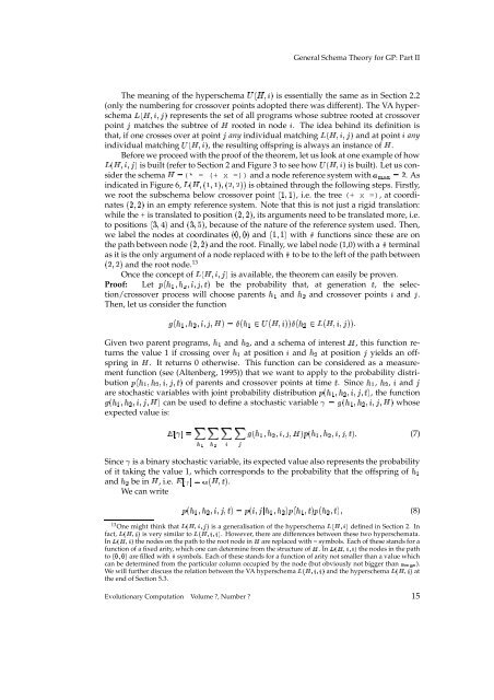
Before we proceed with the proof of the theorem, let us look at one example of how
��¥ £¨§���§���� is built (refer to Section 2 and Figure 3 to see how ��¥ £¨§���� is built). Let us consider
the schema £�� (* = (+ x =)) and a node reference system with ����������� . As
indicated in Figure 6, ��¥ £¨§ ¥ ��§�����§ ¥ ��§������ is obtained through the following steps. Firstly,
we root the subschema below crossover point ¥ ��§���� , i.e. the tree (+ x =), at coordinates
¥ ��§���� in an empty reference system. Note that this is not just a rigid translation:
while the + is translated to position ¥ ��§���� , its arguments need to be translated more, i.e.
to positions ¥ ��§���� and ¥ ��§���� , because of the nature of the reference system used. Then,
we label the nodes at coordinates ¥�� § � � and ¥ ��§���� with # functions since these are on
the path between node ¥ ��§���� and the root. Finally, we label node (1,0) with a # terminal
as it is the only argument of a node replaced with # to be to the left of the path between
¥ ��§���� and the root node. 13
Once the concept of ��¥ £�§���§���� is available, the theorem can easily be proven.
Proof: Let � ¥�� � § � � §���§���§�©�� be the probability that, at generation © , the selection/crossover
process will choose parents � � and � � and crossover points � and � .
Then, let us consider the function
��¥���� § ��� §���§���§�£���� � ¥���������¥ £¨§������ � ¥������¨��¥ £¨§���§��������
Given two parent programs, � � and � � , and a schema of interest £ , this function returns
the value 1 if crossing over � � at position � and � � at position � yields an offspring
in £ . It returns 0 otherwise. This function can be considered as a measurement
function (see (Altenberg, 1995)) that we want to apply to the probability distribution
� ¥���� § ��� §���§���§�©�� of parents and crossover points at time © . Since ��� , ��� , � and �
are stochastic variables with joint probability distribution � ¥���� § ��� §���§���§�©�� , the function
��¥���� § ��� §���§���§�£�� can be used to define a stochastic variable ��� ��¥���� § ��� §���§���§�£�� whose
expected value is:
�������������������
���
�
� � ��¥�� � § � � §���§���§�£���� ¥�� � § � � §���§���§�©���� (7)
� Since is a binary stochastic variable, its expected value also represents the probability
of it taking the value 1, which corresponds to the probability that the offspring of
and ��� be £ in , i.e. ��� ¥ £¨§�©�� . �������
We can write
¥���� § ��� §���§���§�©����¦� ¥ ��§���� ��� § ��� ��� ¥���� §�©���� ¥���� §�©���§ (8)
�
13One might think ��������������� that is a generalisation of the ����������� hyperschema defined in Section 2. In
����������� fact, is very similar ��������������� to . However, there are differences between these two hyperschemata.
����������� In the nodes on the path to the root node � in are replaced with = symbols. Each of these stands for a
function of a fixed arity, which one can determine from the structure � of . ��������������� In the nodes in the path
��������� to are filled with # symbols. Each of these stands for a function of arity not smaller than a value which
can be determined from the particular column occupied by the node (but obviously not bigger ������� than ).
We will further discuss the relation between the VA ��������������� hyperschema and the ����������� hyperschema at
the end of Section 5.3.
Evolutionary Computation Volume ?, Number ? 15
� �