Programación Lineal, una revisión del Simplex desde el Álgebra ...
Programación Lineal, una revisión del Simplex desde el Álgebra ...
Programación Lineal, una revisión del Simplex desde el Álgebra ...

You also want an ePaper? Increase the reach of your titles
YUMPU automatically turns print PDFs into web optimized ePapers that Google loves.
<strong>Programación</strong><br />
<strong>Lineal</strong>, <strong>una</strong><br />
<strong>revisión</strong> <strong>d<strong>el</strong></strong><br />
<strong>Simplex</strong> <strong>desde</strong><br />
<strong>el</strong> <strong>Álgebra</strong><br />
<strong>Lineal</strong><br />
Departamento<br />
de<br />
Matemáticas<br />
Intro<br />
Ejemplo<br />
SB<br />
SBF<br />
Óptimos<br />
<strong>Simplex</strong><br />
Saliente<br />
Optimalidad<br />
<strong>Programación</strong> <strong>Lineal</strong>, <strong>una</strong> <strong>revisión</strong> <strong>d<strong>el</strong></strong><br />
<strong>Simplex</strong> <strong>desde</strong> <strong>el</strong> <strong>Álgebra</strong> <strong>Lineal</strong><br />
Departamento de Matemáticas
<strong>Programación</strong><br />
<strong>Lineal</strong>, <strong>una</strong><br />
<strong>revisión</strong> <strong>d<strong>el</strong></strong><br />
<strong>Simplex</strong> <strong>desde</strong><br />
<strong>el</strong> <strong>Álgebra</strong><br />
<strong>Lineal</strong><br />
Departamento<br />
de<br />
Matemáticas<br />
Intro<br />
Ejemplo<br />
SB<br />
SBF<br />
Óptimos<br />
<strong>Simplex</strong><br />
Saliente<br />
Optimalidad<br />
En esta presentación veremos cómo se resu<strong>el</strong>ve un problema de<br />
programación mediante <strong>el</strong> algoritmo <strong>Simplex</strong> desarrollado por<br />
G. Dantzing. Enfatizaremos los conceptos <strong>d<strong>el</strong></strong> álgebra lineal<br />
cuando revisemos <strong>el</strong> algoritmo.
<strong>Programación</strong><br />
<strong>Lineal</strong>, <strong>una</strong><br />
<strong>revisión</strong> <strong>d<strong>el</strong></strong><br />
<strong>Simplex</strong> <strong>desde</strong><br />
<strong>el</strong> <strong>Álgebra</strong><br />
<strong>Lineal</strong><br />
Departamento<br />
de<br />
Matemáticas<br />
Intro<br />
Ejemplo<br />
SB<br />
SBF<br />
Óptimos<br />
<strong>Simplex</strong><br />
Saliente<br />
Optimalidad<br />
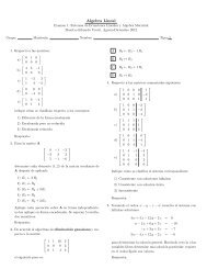
Ejemplo<br />
Consideremos <strong>el</strong> siguiente problema:<br />
Max w = 15 x + 25 y + 19 z<br />
sujeto a las condiciones<br />
x + 2 y + 2 z ≤ 2<br />
2 x + y + z ≤ 2<br />
x + 5 y + z ≤ 3<br />
z ≤ 0.8<br />
con x, y, z ≥ 0.
<strong>Programación</strong><br />
<strong>Lineal</strong>, <strong>una</strong><br />
<strong>revisión</strong> <strong>d<strong>el</strong></strong><br />
<strong>Simplex</strong> <strong>desde</strong><br />
<strong>el</strong> <strong>Álgebra</strong><br />
<strong>Lineal</strong><br />
Departamento<br />
de<br />
Matemáticas<br />
Intro<br />
Ejemplo<br />
SB<br />
SBF<br />
Óptimos<br />
<strong>Simplex</strong><br />
Saliente<br />
Optimalidad<br />
Ejemplo<br />
Consideremos <strong>el</strong> siguiente problema:<br />
Max w = 15 x + 25 y + 19 z<br />
sujeto a las condiciones<br />
x + 2 y + 2 z ≤ 2<br />
2 x + y + z ≤ 2<br />
x + 5 y + z ≤ 3<br />
z ≤ 0.8<br />
con x, y, z ≥ 0. La forma estándar de este problema es:<br />
Max w = 15 x + 25 y + 19 z<br />
sujeto a las condiciones<br />
x + 2 y + 2 z + s1 = 2<br />
2 x + y + z + s2 = 2<br />
x + 5 y + z + s3 = 3<br />
z + s4 = 0.8<br />
con x, y, z, s1, s2, s3, s4 ≥ 0.
<strong>Programación</strong><br />
<strong>Lineal</strong>, <strong>una</strong><br />
<strong>revisión</strong> <strong>d<strong>el</strong></strong><br />
<strong>Simplex</strong> <strong>desde</strong><br />
<strong>el</strong> <strong>Álgebra</strong><br />
<strong>Lineal</strong><br />
Departamento<br />
de<br />
Matemáticas<br />
Intro<br />
Ejemplo<br />
SB<br />
SBF<br />
Óptimos<br />
<strong>Simplex</strong><br />
Saliente<br />
Optimalidad<br />
La forma estándar se puede escribir en forma matricial como:<br />
de manera que<br />
⎡<br />
⎢<br />
⎣<br />
Max w = 15 x + 25 y + 19 z<br />
1 2 2 1 0 0 0<br />
2 1 1 0 1 0 0<br />
1 5 1 0 0 1 0<br />
0 0 1 0 0 0 1<br />
con x, y, z, s1, s2, s3, s4 ≥ 0.<br />
⎛<br />
⎤ ⎜<br />
⎥ ⎜<br />
⎥ ⎜<br />
⎦ ⎜<br />
⎝<br />
x<br />
y<br />
z<br />
s1<br />
s2<br />
s3<br />
s4<br />
⎞<br />
⎟ ⎛ ⎞<br />
⎟<br />
2<br />
⎟ ⎜<br />
⎟ = ⎜ 2 ⎟<br />
⎝<br />
⎟ 3 ⎠<br />
⎟<br />
⎠ 0.8
<strong>Programación</strong><br />
<strong>Lineal</strong>, <strong>una</strong><br />
<strong>revisión</strong> <strong>d<strong>el</strong></strong><br />
<strong>Simplex</strong> <strong>desde</strong><br />
<strong>el</strong> <strong>Álgebra</strong><br />
<strong>Lineal</strong><br />
Departamento<br />
de<br />
Matemáticas<br />
Intro<br />
Ejemplo<br />
SB<br />
SBF<br />
Óptimos<br />
<strong>Simplex</strong><br />
Saliente<br />
Optimalidad<br />
Desde <strong>el</strong> punto de vista <strong>d<strong>el</strong></strong> álgebra lineal, <strong>el</strong> problema consiste<br />
en<br />
Max w = 15 x + 25 y + 19 z + 0 s1 + 0 s2 + 0 s3 + 0 s4<br />
donde las variables son los coeficientes de la combinación lineal:<br />
donde:<br />
x a1 + y a2 + z a3 + s1 a4 + s2 a5 + s3 a6 + s4 a7 = b<br />
[a1 a2 a3 a4 a5 a6 a7 ] =<br />
⎡<br />
⎢<br />
⎣<br />
1 2 2 1 0 0 0<br />
2 1 1 0 1 0 0<br />
1 5 1 0 0 1 0<br />
0 0 1 0 0 0 1<br />
⎤<br />
⎛<br />
⎞<br />
⎥ ⎜<br />
⎥<br />
⎦ , b = ⎜<br />
⎝<br />
2<br />
2<br />
3<br />
0.8<br />
⎟<br />
⎠<br />
con x, y, z, s1, s2, s3, s4 ≥ 0. Es decir, los coeficientes de la<br />
combinación lineal no deben ser negativos.
<strong>Programación</strong><br />
<strong>Lineal</strong>, <strong>una</strong><br />
<strong>revisión</strong> <strong>d<strong>el</strong></strong><br />
<strong>Simplex</strong> <strong>desde</strong><br />
<strong>el</strong> <strong>Álgebra</strong><br />
<strong>Lineal</strong><br />
Departamento<br />
de<br />
Matemáticas<br />
Intro<br />
Ejemplo<br />
SB<br />
SBF<br />
Óptimos<br />
<strong>Simplex</strong><br />
Saliente<br />
Optimalidad<br />
Solución Básica<br />
Trabajemos un poco con sólo las restricciones. Para un sistema<br />
de ecuaciones lineales consistente y con infinitas soluciones<br />
⎛ ⎞<br />
⎜<br />
A x = [a1 · · · an] ⎝<br />
x1<br />
.<br />
xn<br />
⎟<br />
⎠ = b, A ∈ Mm×n<br />
diremos que <strong>una</strong> solución xo =< c1, . . . , cn > es <strong>una</strong> solución<br />
básica, si es posible escoger <strong>d<strong>el</strong></strong> conjunto formado por las<br />
columnas de A<br />
{a1, a2, . . . , an}<br />
<strong>una</strong> base de R m y los coeficientes de la combinación lineal de<br />
<strong>el</strong>la que dan b son los correspondientes valores de xo y los<br />
restantes (los coeficientes de la combinación lineal asociados a<br />
las columnas que no se escogieron para formar la base) son<br />
cero. Concluimos que en <strong>una</strong> solución básica, debe haber por lo<br />
menos n − m variables cero (pues las columnas están en R m ).
<strong>Programación</strong><br />
<strong>Lineal</strong>, <strong>una</strong><br />
<strong>revisión</strong> <strong>d<strong>el</strong></strong><br />
<strong>Simplex</strong> <strong>desde</strong><br />
<strong>el</strong> <strong>Álgebra</strong><br />
<strong>Lineal</strong><br />
Departamento<br />
de<br />
Matemáticas<br />
Intro<br />
Ejemplo<br />
SB<br />
SBF<br />
Óptimos<br />
<strong>Simplex</strong><br />
Saliente<br />
Optimalidad<br />
Siguiendo con nuestro ejemplo, tenemos varias soluciones<br />
básicas:<br />
(x = 0, y = 0, z = 0, s1 = 2, s2 = 2, s3 = 3, s4 = 0.8)<br />
Pues de<br />
⎛<br />
⎜<br />
a1 = ⎜<br />
⎝<br />
1<br />
2<br />
1<br />
0<br />
⎞<br />
⎛<br />
⎟<br />
⎠ a2<br />
⎜<br />
= ⎜<br />
⎝<br />
2<br />
1<br />
5<br />
0<br />
⎞<br />
⎛<br />
⎟<br />
⎠ a3<br />
⎜<br />
= ⎜<br />
⎝<br />
2<br />
1<br />
1<br />
1<br />
⎞<br />
⎛<br />
⎟<br />
⎠ a4<br />
⎜<br />
= ⎜<br />
⎝<br />
1<br />
0<br />
0<br />
0<br />
⎞<br />
⎛<br />
⎟<br />
⎠ a5<br />
⎜<br />
= ⎜<br />
⎝<br />
0<br />
1<br />
0<br />
0<br />
⎞<br />
⎛<br />
⎟<br />
⎠ a6<br />
⎜<br />
= ⎜<br />
⎝<br />
0<br />
0<br />
1<br />
0<br />
⎞<br />
⎛<br />
⎟<br />
⎠ a7<br />
⎜<br />
= ⎜<br />
⎝<br />
El conjunto {a4, a5, a6, a7} es <strong>una</strong> base para R 4 y al resolver<br />
s1a4 + s2 a5 + s3 a6 + s4 a7 = [a4 a5 a6 a7]<br />
se obtiene s1 = 2, s2 = 2, s3 = 3, s4 = 0.8<br />
⎛<br />
⎜<br />
⎝<br />
s1<br />
s2<br />
s3<br />
s4<br />
⎞<br />
⎟<br />
⎠ =<br />
⎛<br />
⎜<br />
⎝<br />
2<br />
2<br />
3<br />
0.8<br />
0<br />
0<br />
0<br />
1<br />
⎞<br />
⎟<br />
⎠<br />
⎞<br />
⎟<br />
⎠
<strong>Programación</strong><br />
<strong>Lineal</strong>, <strong>una</strong><br />
<strong>revisión</strong> <strong>d<strong>el</strong></strong><br />
<strong>Simplex</strong> <strong>desde</strong><br />
<strong>el</strong> <strong>Álgebra</strong><br />
<strong>Lineal</strong><br />
Departamento<br />
de<br />
Matemáticas<br />
Intro<br />
Ejemplo<br />
SB<br />
SBF<br />
Óptimos<br />
<strong>Simplex</strong><br />
Saliente<br />
Optimalidad<br />
(x = 19/45, y = 16/45, z = 4/5, s1 = −11/15, s2 = 0, s3 = 0, s4 = 0)<br />
es <strong>una</strong> solución básica.<br />
Pues <strong>el</strong> conjunto {a1, a2, a3, a4} es <strong>una</strong> base para R4 y al<br />
resolver<br />
⎜<br />
x a1 + y a2 + z a3 + s1 a4 = [a1 a2 a3 a4] ⎜<br />
⎝<br />
⎛<br />
x<br />
y<br />
z<br />
s1<br />
⎞<br />
⎟<br />
⎠ =<br />
⎛<br />
⎜<br />
⎝<br />
se obtiene x = 19/45, y = 16/45, z = 4/5, s1 = −11/15<br />
2<br />
2<br />
3<br />
0.8<br />
⎞<br />
⎟<br />
⎠
<strong>Programación</strong><br />
<strong>Lineal</strong>, <strong>una</strong><br />
<strong>revisión</strong> <strong>d<strong>el</strong></strong><br />
<strong>Simplex</strong> <strong>desde</strong><br />
<strong>el</strong> <strong>Álgebra</strong><br />
<strong>Lineal</strong><br />
Departamento<br />
de<br />
Matemáticas<br />
Intro<br />
Ejemplo<br />
SB<br />
SBF<br />
Óptimos<br />
<strong>Simplex</strong><br />
Saliente<br />
Optimalidad<br />
(x = −4/5, y = 3/5, z = 4/5, s2 = 11/5, s1 = 0, s3 = 0, s4 = 0) es<br />
<strong>una</strong> solución básica.<br />
Pues <strong>el</strong> conjunto {a1, a2, a3, a5} es <strong>una</strong> base para R4 y al<br />
resolver<br />
⎜<br />
x a1 + y a2 + z a3 + s2 a5 = [a1 a2 a3 a5] ⎜<br />
⎝<br />
⎛<br />
x<br />
y<br />
z<br />
s2<br />
⎞<br />
⎟<br />
⎠ =<br />
se obtiene x = −4/5, y = 3/5, z = 4/5, s2 = 11/5<br />
⎛<br />
⎜<br />
⎝<br />
2<br />
2<br />
3<br />
0.8<br />
⎞<br />
⎟<br />
⎠
<strong>Programación</strong><br />
<strong>Lineal</strong>, <strong>una</strong><br />
<strong>revisión</strong> <strong>d<strong>el</strong></strong><br />
<strong>Simplex</strong> <strong>desde</strong><br />
<strong>el</strong> <strong>Álgebra</strong><br />
<strong>Lineal</strong><br />
Departamento<br />
de<br />
Matemáticas<br />
Intro<br />
Ejemplo<br />
SB<br />
SBF<br />
Óptimos<br />
<strong>Simplex</strong><br />
Saliente<br />
Optimalidad<br />
Correspondencia 1<br />
De acuerdo a la definición de solución básica, hay <strong>una</strong><br />
correspondencia entre soluciones básicas de A x = b y<br />
s<strong>el</strong>ecciones de las columnas de A para ser <strong>una</strong> base de R m .<br />
Observe también que no siempre que se s<strong>el</strong>eccionen m<br />
columnas de A tendremos <strong>una</strong> base para R m . Haciendo<br />
cálculos, <strong>el</strong> número de posibles s<strong>el</strong>ecciones de m <strong>el</strong>ementos de<br />
un conjunto con n en total será:<br />
número de posibles bases =<br />
n<br />
m<br />
<br />
=<br />
n!<br />
(n − m)! m!<br />
Por ejemplo, si continuamos con nuestro problema; m = 4, n = 7, <strong>el</strong> número de posibles s<strong>el</strong>ecciones de<br />
bases de R 4 de las columnas de A es 35 y haciendo <strong>una</strong> <strong>revisión</strong> exhaustiva las siguientes s<strong>el</strong>ecciones<br />
no darán <strong>una</strong> base para R 3 :<br />
• {a1, a2, a4, a5}<br />
• {a1, a2, a4, a6}<br />
• {a1, a2, a5, a6}<br />
• {a1, a4, a5, a6}<br />
• {a2, a3, a6, a7}
<strong>Programación</strong><br />
<strong>Lineal</strong>, <strong>una</strong><br />
<strong>revisión</strong> <strong>d<strong>el</strong></strong><br />
<strong>Simplex</strong> <strong>desde</strong><br />
<strong>el</strong> <strong>Álgebra</strong><br />
<strong>Lineal</strong><br />
Departamento<br />
de<br />
Matemáticas<br />
Intro<br />
Ejemplo<br />
SB<br />
SBF<br />
Óptimos<br />
<strong>Simplex</strong><br />
Saliente<br />
Optimalidad<br />
SBF<br />
Si regresamos al problema de programación lineal, donde se<br />
requiere que los coeficientes de la combinación lineal sean no<br />
negativos (≥ 0), no estamos interesados en todas las soluciones<br />
básicas; descartaremos aqu<strong>el</strong>las soluciones básicas que tienen<br />
uno o varios valores negativos. Diremos que <strong>una</strong> solución<br />
básica xo es <strong>una</strong> solución básica factible (SBF) a A x = b, si xo<br />
no tiene componentes negativas.<br />
Si regresamos a nuestro problema; revisando exhaustivamente<br />
de las 30 s<strong>el</strong>ecciones que dan SBs, las únicas SBFs son:<br />
• SBF1(a1, a2, a3, a7): x = 2/3, y = 5/12, z = 1/4, s4 = 11/20, s1 = 0, s2 = 0, s3 = 0<br />
• SBF2(a1, a2, a4, a7):x = 7/9, y = 4/9, s1 = 1/3, s4 = 4/5, z = 0, s2 = 0, s3 = 0<br />
• SBF3(a1, a3, a5, a7):x = 2/5, z = 4/5, s2 = 2/5, s3 = 9/5, y = 0, s1 = 0, s4 = 0<br />
• SBF4(a1, a3, a6, a7):x = 2/3, z = 2/3, s3 = 5/3, s4 = 2/15, y = 0, s1 = 0, s2 = 0<br />
• SBF5(a1, a4, a6, a7):x = 1, s1 = 1, s3 = 2, s4 = 4/5, y = 0, z = 0, s2 = 0<br />
• SBF6(a2, a3, a5, a6):y = 1/5, z = 4/5, s2 = 1, s3 = 6/5, x = 0, s1 = 0, s4 = 0<br />
• SBF7(a2, a3, a5, a7):y = 1/2, z = 1/2, s2 = 1, s4 = 3/10, x = 0, s1 = 0, s3 = 0<br />
• SBF8(a2, a4, a5, a7):y = 3/5, s1 = 4/5, s2 = 7/5, s4 = 4/5, x = 0, z = 0, s3 = 0<br />
• SBF9(a3, a4, a5, a7):z = 4/5, s1 = 2/5, s2 = 6/5, s3 = 11/5, x = 0, y = 0, s4 = 0<br />
• SBF10(a4, a5, a6, a7):s1 = 2, s2 = 2, s3 = 3, s4 = 4/5, x = 0, y = 0, z = 0
<strong>Programación</strong><br />
<strong>Lineal</strong>, <strong>una</strong><br />
<strong>revisión</strong> <strong>d<strong>el</strong></strong><br />
<strong>Simplex</strong> <strong>desde</strong><br />
<strong>el</strong> <strong>Álgebra</strong><br />
<strong>Lineal</strong><br />
Departamento<br />
de<br />
Matemáticas<br />
Intro<br />
Ejemplo<br />
SB<br />
SBF<br />
Óptimos<br />
<strong>Simplex</strong><br />
Saliente<br />
Optimalidad<br />
Si ahora graficamos todos los puntos de R 3 que satisfacen las<br />
restricciones y que tienen componentes no negativas y también<br />
tomamos las soluciones básicas factibles y graficamos de éstas<br />
sólo las componentes x, y y z obtenemos la siguiente gráfica.
<strong>Programación</strong><br />
<strong>Lineal</strong>, <strong>una</strong><br />
<strong>revisión</strong> <strong>d<strong>el</strong></strong><br />
<strong>Simplex</strong> <strong>desde</strong><br />
<strong>el</strong> <strong>Álgebra</strong><br />
<strong>Lineal</strong><br />
Departamento<br />
de<br />
Matemáticas<br />
Intro<br />
Ejemplo<br />
SB<br />
SBF<br />
Óptimos<br />
<strong>Simplex</strong><br />
Saliente<br />
Optimalidad<br />
Correspondencia 2<br />
El ejemplo anterior ilustra un resultado clave en programación<br />
lineal<br />
Existe <strong>una</strong> correspondencia entre las soluciones<br />
básicas factibles y los puntos extremos o esquinas de<br />
la región factible (la totalidad de puntos que cumplen<br />
las restricciones, incluida la no negatividad)
<strong>Programación</strong><br />
<strong>Lineal</strong>, <strong>una</strong><br />
<strong>revisión</strong> <strong>d<strong>el</strong></strong><br />
<strong>Simplex</strong> <strong>desde</strong><br />
<strong>el</strong> <strong>Álgebra</strong><br />
<strong>Lineal</strong><br />
Departamento<br />
de<br />
Matemáticas<br />
Intro<br />
Ejemplo<br />
SB<br />
SBF<br />
Óptimos<br />
<strong>Simplex</strong><br />
Saliente<br />
Optimalidad<br />
Adyacencia<br />
Más aún: si revisamos en la gráfica de la región factible, puntos<br />
extremos que son adyacentes en <strong>el</strong> sentido que los une un lado<br />
<strong>d<strong>el</strong></strong> poliedro, vemos que los puntos extremos están asociados a<br />
bases para R m que tienen prácticamente las mismas columnas<br />
de A difiriendo sólo en 1. Por ejemplo:<br />
• P3(x = 2/5, y = 0, z = 4/5) que proviene de la SBF3<br />
asociada a la base {a1, a3, a5, a7} sí es adyacente a<br />
P4(x = 2/3, y = 0, z = 2/3) que proviene de la SBF4<br />
asociada a la base {a1, a3, a6, a7}.<br />
• P6(x = 0, y = 1/5, z = 4/5) que proviene de la SBF6<br />
asociada a la base {a2, a3, a5, a6} no es adyacente a<br />
P1(x = 2/3, y = 5/12, z = 1/4) que proviene de la SBF1<br />
asociada a la base {a1, a2, a3, a7}.
<strong>Programación</strong><br />
<strong>Lineal</strong>, <strong>una</strong><br />
<strong>revisión</strong> <strong>d<strong>el</strong></strong><br />
<strong>Simplex</strong> <strong>desde</strong><br />
<strong>el</strong> <strong>Álgebra</strong><br />
<strong>Lineal</strong><br />
Departamento<br />
de<br />
Matemáticas<br />
Intro<br />
Ejemplo<br />
SB<br />
SBF<br />
Óptimos<br />
<strong>Simplex</strong><br />
Saliente<br />
Optimalidad<br />
• P1(2/3, 5/12, 1/4) − SBF1 − {a1, a2, a3, a7}<br />
• P2(7/9, 4/9, 0) − SBF2 − {a1, a2, a4, a7}<br />
• P3(2/5, 0, 4/5) − SBF3 − {a1, a3, a5, a7}<br />
• P4(2/3, 0, 2/3)) − SBF4 − {a1, a3, a6, a7}<br />
• P5(1, 0, 0) − SBF5 − {a1, a4, a6, a7}<br />
• P6(0, 1/5, 4/5) − SBF6 − {a2, a3, a5, a6}<br />
• P7(0, 1/2, 1/2) − SBF7 − {a2, a3, a5, a7}<br />
• P8(0, 3/5, 0) − SBF8 − {a2, a4, a5, a7}<br />
• P9(0, 0, 4/5) − SBF9 − {a3, a4, a5, a7}<br />
• P10(0, 0, 0) − SBF10 − {a4, a5, a6, a7}
<strong>Programación</strong><br />
<strong>Lineal</strong>, <strong>una</strong><br />
<strong>revisión</strong> <strong>d<strong>el</strong></strong><br />
<strong>Simplex</strong> <strong>desde</strong><br />
<strong>el</strong> <strong>Álgebra</strong><br />
<strong>Lineal</strong><br />
Departamento<br />
de<br />
Matemáticas<br />
Intro<br />
Ejemplo<br />
SB<br />
SBF<br />
Óptimos<br />
<strong>Simplex</strong><br />
Saliente<br />
Optimalidad<br />
Optimizando<br />
Consideremos a ahora la función lineal. Como en <strong>una</strong> variable,<br />
Toda función lineal definida sobre un segmento de<br />
recta alzanca sus valores óptimos (máximo o mínimo)<br />
en los puntos extremos <strong>d<strong>el</strong></strong> segmento.<br />
El caso más trivial ocurre cuando la función lineal es de valor<br />
constante en <strong>el</strong> segmento de recta. Pero aún en este caso, no<br />
hay contradicción al decir que los óptimos los alcanza en los<br />
extremos (aún cuando también los alcanza en todos los puntos<br />
<strong>d<strong>el</strong></strong> segmento).<br />
Si nos traemos este resultado a programación lineal:<br />
Todo problema de programación lineal que tiene<br />
región factible acotada tendrá su máximo y su<br />
mínimo en un punto extremo (esquina <strong>d<strong>el</strong></strong> poliedro).<br />
Por este resultado, las soluciones básicas factibles serán claves<br />
para resolver un PL.
<strong>Programación</strong><br />
<strong>Lineal</strong>, <strong>una</strong><br />
<strong>revisión</strong> <strong>d<strong>el</strong></strong><br />
<strong>Simplex</strong> <strong>desde</strong><br />
<strong>el</strong> <strong>Álgebra</strong><br />
<strong>Lineal</strong><br />
Departamento<br />
de<br />
Matemáticas<br />
Intro<br />
Ejemplo<br />
SB<br />
SBF<br />
Óptimos<br />
<strong>Simplex</strong><br />
Saliente<br />
Optimalidad<br />
El <strong>Simplex</strong><br />
El Algoritmo <strong>Simplex</strong> desarrollado en en 1947 por George<br />
Bernard Dantzig (8 de noviembre de 1914-13 de mayo de 2005)<br />
es un algoritmo para resolver problemas de programación lineal<br />
y consiste en<br />
Iniciando en <strong>una</strong> esquina <strong>d<strong>el</strong></strong> poliedro (solución<br />
básica factible), <strong>el</strong> algoritmo <strong>Simplex</strong> recorre parte de<br />
las esquinas <strong>d<strong>el</strong></strong> poliedro hasta llegar a la óptima. El<br />
algoritmo pasa de <strong>una</strong> SBF a otra SBF adyacente con<br />
<strong>una</strong> evaluación mejor.<br />
Las claves serán: Dada <strong>una</strong> SBF, ¿cómo escoger otra SBF<br />
adyacente? y ¿cómo cambiar de <strong>una</strong> SBF a otra SBF<br />
eficientemente?
<strong>Programación</strong><br />
<strong>Lineal</strong>, <strong>una</strong><br />
<strong>revisión</strong> <strong>d<strong>el</strong></strong><br />
<strong>Simplex</strong> <strong>desde</strong><br />
<strong>el</strong> <strong>Álgebra</strong><br />
<strong>Lineal</strong><br />
Departamento<br />
de<br />
Matemáticas<br />
Intro<br />
Ejemplo<br />
SB<br />
SBF<br />
Óptimos<br />
<strong>Simplex</strong><br />
Saliente<br />
Optimalidad<br />
variables entrante y saliente<br />
Por conveniencia, indicaremos cuáles son las columnas de A<br />
que forman la base indicando las variables asociadas a <strong>el</strong>la:<br />
En <strong>una</strong> SBF, a las variables que son coeficientes de<br />
las columnas que pertenecen a <strong>una</strong> base de la SBF les<br />
llamaremos variables básicas; a las otras les<br />
llamaremos variables no básicas.<br />
Un poco más de nomenclatura:<br />
Cuando se pasa de <strong>una</strong> SBF a otra SBF adyacente<br />
sólo <strong>una</strong> columna de A cambia en la base: a la<br />
variable asociada a la columna de A que deja la base<br />
se le llama variable básica saliente; a la variable<br />
asociada a la columna de A que ingresa reemplazando<br />
a la saliente se le llama variable básica entrante.
<strong>Programación</strong><br />
<strong>Lineal</strong>, <strong>una</strong><br />
<strong>revisión</strong> <strong>d<strong>el</strong></strong><br />
<strong>Simplex</strong> <strong>desde</strong><br />
<strong>el</strong> <strong>Álgebra</strong><br />
<strong>Lineal</strong><br />
Departamento<br />
de<br />
Matemáticas<br />
Intro<br />
Ejemplo<br />
SB<br />
SBF<br />
Óptimos<br />
<strong>Simplex</strong><br />
Saliente<br />
Optimalidad<br />
Regresemos a nuestro problema inicial. La matriz aumentada<br />
inicial de las restricciones [A|b] (reconociendo que a4, a5, a6 y<br />
a7 constituyen <strong>una</strong> base para R 4 ) puede ser escrita como:<br />
⎡<br />
⎤<br />
x y z s1 s2 s3 s4 rhs vb<br />
⎢<br />
⎥<br />
⎢<br />
⎥<br />
⎢<br />
⎥<br />
⎢<br />
⎥<br />
⎢<br />
⎥<br />
⎣<br />
⎦<br />
1 2 2 1 0 0 0 2 s1<br />
2 1 1 0 1 0 0 2 s2<br />
1 5 1 0 0 1 0 3 s3<br />
0 0 1 0 0 0 1 4/5 s4<br />
La última columna adicional, que no se utiliza en álgebra lineal<br />
en la aumentada, es conveniente en programación lineal por<br />
que ayuda a ubicar la SBF (y por tanto, la base para R m<br />
extraída de las columnas de A). Observe además que<br />
• b = 2 · a4 + 2 a5 + 3 a6 + 4/5 a7<br />
• a1 = 1 · a4 + 2 a5 + 1 a6 + 0 a7<br />
• a2 = 2 · a4 + 1 a5 + 5 a6 + 0 a7<br />
• a3 = 2 · a4 + 1 a5 + 1 a6 + 1 a7
<strong>Programación</strong><br />
<strong>Lineal</strong>, <strong>una</strong><br />
<strong>revisión</strong> <strong>d<strong>el</strong></strong><br />
<strong>Simplex</strong> <strong>desde</strong><br />
<strong>el</strong> <strong>Álgebra</strong><br />
<strong>Lineal</strong><br />
Departamento<br />
de<br />
Matemáticas<br />
Intro<br />
Ejemplo<br />
SB<br />
SBF<br />
Óptimos<br />
<strong>Simplex</strong><br />
Saliente<br />
Optimalidad<br />
Regresando a nuestro problema: En la solución actual x es <strong>una</strong><br />
variable no básica (a1 no está en la base). Supongamos que<br />
queremos aumentar <strong>el</strong> valor de x, es decir, queremos que a1<br />
entre a la base actual. Pivoteando mediante operaciones de<br />
renglón podemos ver a qué SBF nos puede llevar al<br />
intercambiar por las columnas de A que están en la base:
<strong>Programación</strong><br />
<strong>Lineal</strong>, <strong>una</strong><br />
<strong>revisión</strong> <strong>d<strong>el</strong></strong><br />
<strong>Simplex</strong> <strong>desde</strong><br />
<strong>el</strong> <strong>Álgebra</strong><br />
<strong>Lineal</strong><br />
Departamento<br />
de<br />
Matemáticas<br />
Intro<br />
Ejemplo<br />
SB<br />
SBF<br />
Óptimos<br />
<strong>Simplex</strong><br />
Saliente<br />
Optimalidad<br />
⎡<br />
⎣<br />
1) Cambiando a1 por a4 (es decir, x por s1): No da <strong>una</strong> SBF.<br />
Esto equivale a hacer 1 en la posición <strong>d<strong>el</strong></strong> renglón 1 (por s1) y<br />
columna 1 (por x) y posteriormente hacer ceros abajo y arriba)<br />
1. R2 ← R2 − 2 R1<br />
2. R3 ← R3 − 1 R1<br />
Actual Nueva<br />
SBF10<br />
⎤ ⎡<br />
SB<br />
x y z s1 s2 s3 s4 rhs vb<br />
1 2 2 1 0 0 0 2 s1<br />
2 1 1 0 1 0 0 2 s2<br />
1 5 1 0 0 1 0 3 s3<br />
0 0 1 0 0 0 1 4/5 s4<br />
b = 2 · a4 + 2 a5 + 3 a6 + 4/5 a7<br />
a1 = 1 · a4 + 2 a5 + 1 a6 + 0 a7<br />
a2 = 2 · a4 + 1 a5 + 5 a6 + 0 a7<br />
a3 = 2 · a4 + 1 a5 + 1 a6 + 1 a7<br />
⎦<br />
⎣<br />
x y z s1 s2 s3 s4 rhs vb<br />
1 2 2 1 0 0 0 2 x<br />
0 −3 −3 −2 1 0 0 −2 s2<br />
0 3 −1 −1 0 1 0 1 s3<br />
0 0 1 0 0 0 1 4/5 s4<br />
b = 2 · a1 − 2 a5 + 1 a6 + 4/5 a7<br />
a2 = 2 · a1 − 3 a5 + 3 a6 + 0 a7<br />
a3 = 2 · a1 − 3 a5 − 1 a6 + 1 a7<br />
a4 = 1 · a1 − 2 a5 − 1 a6 + 0 a7<br />
⎤<br />
⎦
<strong>Programación</strong><br />
<strong>Lineal</strong>, <strong>una</strong><br />
<strong>revisión</strong> <strong>d<strong>el</strong></strong><br />
<strong>Simplex</strong> <strong>desde</strong><br />
<strong>el</strong> <strong>Álgebra</strong><br />
<strong>Lineal</strong><br />
Departamento<br />
de<br />
Matemáticas<br />
Intro<br />
Ejemplo<br />
SB<br />
SBF<br />
⎡<br />
Óptimos<br />
⎣<br />
2) Cambiando a1 por a5: Sí da <strong>una</strong> SBF<br />
<strong>Simplex</strong><br />
1<br />
2<br />
2<br />
1<br />
2<br />
1<br />
1<br />
0<br />
0<br />
1<br />
0<br />
0<br />
0<br />
0<br />
2<br />
2<br />
s1<br />
s2<br />
Saliente 1 5 1 0 0 1 0 3 s3<br />
0<br />
Optimalidad<br />
0 1 0 0 0 1 4/5 s4<br />
1. R2 ← 1<br />
2 R2<br />
2. R1 ← R1 − 1 R2<br />
3. R3 ← R3 − 1 R2<br />
Actual Nueva<br />
SBF10<br />
x y z s1 s2 s3 s4 rhs vb<br />
b = 2 · a4 + 2 a5 + 3 a6 + 4/5 a7<br />
a1 = 1 · a4 + 2 a5 + 1 a6 + 0 a7<br />
a2 = 2 · a4 + 1 a5 + 5 a6 + 0 a7<br />
a3 = 2 · a4 + 1 a5 + 1 a6 + 1 a7<br />
⎤<br />
⎦<br />
⎡<br />
⎣<br />
SBF5<br />
x y z s1 s2 s3 s4 rhs vb<br />
0 3/2 3/2 1 −1/2 0 0 1 s1<br />
1 1/2 1/2 0 1/2 0 0 1 x<br />
0 9/2 1/2 0 −1/2 1 0 2 s3<br />
0 0 1 0 0 0 1 4/5 s4<br />
b = 2 · a1 − 2 a5 + 1 a6 + 4/5 a7<br />
a2 = 2 · a1 − 3 a5 + 3 a6 + 0 a7<br />
a3 = 2 · a1 − 3 a5 − 1 a6 + 1 a7<br />
a4 = 1 · a1 − 2 a5 − 1 a6 + 0 a7<br />
⎤<br />
⎦
<strong>Programación</strong><br />
<strong>Lineal</strong>, <strong>una</strong><br />
<strong>revisión</strong> <strong>d<strong>el</strong></strong><br />
<strong>Simplex</strong> <strong>desde</strong><br />
<strong>el</strong> <strong>Álgebra</strong><br />
<strong>Lineal</strong><br />
Departamento<br />
de<br />
Matemáticas<br />
Intro<br />
Ejemplo<br />
SB<br />
SBF<br />
Óptimos<br />
<strong>Simplex</strong><br />
Saliente<br />
⎡<br />
⎣<br />
Optimalidad<br />
2) Cambiando a1 por a6:No da <strong>una</strong> SBF<br />
SBF10<br />
x y z s1 s2 s3 s4 rhs vb<br />
1 2 2 1 0 0 0 2 s1<br />
2 1 1 0 1 0 0 2 s2<br />
1 5 1 0 0 1 0 3 s3<br />
0 0 1 0 0 0 1 4/5 s4<br />
b = 2 · a4 + 2 a5 + 3 a6 + 4/5 a7<br />
a1 = 1 · a4 + 2 a5 + 1 a6 + 0 a7<br />
a2 = 2 · a4 + 1 a5 + 5 a6 + 0 a7<br />
a3 = 2 · a4 + 1 a5 + 1 a6 + 1 a7<br />
1. R1 ← R1 − 1 R3<br />
1. R2 ← R2 − 2 R3<br />
⎤<br />
⎦<br />
⎡<br />
⎣<br />
SBF<br />
x y z s1 s2 s3 s4 rhs vb<br />
0 −3 1 1 0 −1 0 −1 s1<br />
0 −9 −1 0 1 −2 0 −4 s2<br />
1 5 1 0 0 1 0 3 x<br />
0 0 1 0 0 0 1 4/5 s4<br />
b = −1 · a1 − 4 a4 + 3 a5 + 4/5 a7<br />
a2 = −3 · a1 − 9 a4 + 5 a5 + 0 a7<br />
a3 = 1 · a1 − 1 a4 + 1 a5 + 1 a7<br />
a6 = −1 · a1 − 2 a5 + 1 a5 + 0 a7<br />
⎤<br />
⎦
<strong>Programación</strong><br />
<strong>Lineal</strong>, <strong>una</strong><br />
<strong>revisión</strong> <strong>d<strong>el</strong></strong><br />
<strong>Simplex</strong> <strong>desde</strong><br />
<strong>el</strong> <strong>Álgebra</strong><br />
<strong>Lineal</strong><br />
Departamento<br />
de<br />
Matemáticas<br />
Intro<br />
Ejemplo<br />
SB<br />
SBF<br />
Óptimos<br />
<strong>Simplex</strong><br />
Saliente<br />
Optimalidad<br />
Habiendo decidido hacer básica <strong>una</strong> variable no básica, ¿Cómo<br />
saber cuál es la variable básica saliente?: determinando su<br />
máximo crecimiento: esto va a ocurrir cuando se haga <strong>el</strong><br />
primer cero en <strong>una</strong> variable básica. Para <strong>el</strong> cálculo, se requiere<br />
la columna de las constantes positiva y se añade <strong>una</strong> columna<br />
extra a la derecha donde se registran los cocientes o razones<br />
entre los lados derechos y los valores correspondientes de la<br />
columna de la variable entrante cuando éstos son estrictamente<br />
positivos: se descartan negativos o valores cero: El menor<br />
cociente da <strong>el</strong> máximo crecimiento sin que <strong>una</strong> variable básica<br />
se haga negativa; esto ubica la variable básica saliente.<br />
⎡<br />
⎤<br />
x y z s1 s2 s3 s4 rhs vb razón<br />
⎢<br />
⎣<br />
1 2 2 1 0 0 0 2 s1 2/1 = 2<br />
2 1 1 0 1 0 0 2 s2 2/2 = 1<br />
1 5 1 0 0 1 0 3 s3 3/1 = 3<br />
0 0 1 0 0 0 1 4/5 s4 −−<br />
⎥<br />
⎦
<strong>Programación</strong><br />
<strong>Lineal</strong>, <strong>una</strong><br />
<strong>revisión</strong> <strong>d<strong>el</strong></strong><br />
<strong>Simplex</strong> <strong>desde</strong><br />
<strong>el</strong> <strong>Álgebra</strong><br />
<strong>Lineal</strong><br />
Departamento<br />
de<br />
Matemáticas<br />
Intro<br />
Ejemplo<br />
SB<br />
SBF<br />
Óptimos<br />
<strong>Simplex</strong><br />
Saliente<br />
Optimalidad<br />
¿Y cómo se determina la variable entrante? Es la variable no<br />
básica que tiene un mayor impacto sobre la variable que<br />
representa la función objetivo. En la versión completa <strong>d<strong>el</strong></strong><br />
<strong>Simplex</strong>, también la función se piensa como <strong>una</strong> ecuación:<br />
⎡<br />
⎤<br />
w x y z s1 s2 s3 s4 rhs vb<br />
⎢ 1 −15 −25 −19 0 0 0 0 0 w<br />
⎥<br />
⎢<br />
⎣<br />
0 1 2 2 1 0 0 0 2 s1<br />
0 2 1 1 0 1 0 0 2 s2<br />
0 1 5 1 0 0 1 0 3 s3<br />
0 0 0 1 0 0 0 1 4/5 s4<br />
La variable entrante es la variable no básica que tiene <strong>el</strong> mayor<br />
(en valor absoluto) coeficiente negativo (Si <strong>el</strong> problema es de<br />
minimización, es la variable no básica con <strong>el</strong> mayor coeficiente<br />
positivo) en <strong>el</strong> renglón de la función objetivo.<br />
⎥<br />
⎦
<strong>Programación</strong><br />
<strong>Lineal</strong>, <strong>una</strong><br />
<strong>revisión</strong> <strong>d<strong>el</strong></strong><br />
<strong>Simplex</strong> <strong>desde</strong><br />
<strong>el</strong> <strong>Álgebra</strong><br />
<strong>Lineal</strong><br />
Departamento<br />
de<br />
Matemáticas<br />
Intro<br />
Ejemplo<br />
SB<br />
SBF<br />
Óptimos<br />
<strong>Simplex</strong><br />
Saliente<br />
Optimalidad<br />
Estamos en SBF10: La entrante y, la saliente s3:<br />
⎡<br />
w<br />
⎢ 1<br />
⎢ 0<br />
⎢<br />
0<br />
⎣ 0<br />
x<br />
−15<br />
1<br />
2<br />
1<br />
y<br />
−25<br />
2<br />
1<br />
5<br />
z<br />
−19<br />
2<br />
1<br />
1<br />
s1<br />
0<br />
1<br />
0<br />
0<br />
s2<br />
0<br />
0<br />
1<br />
0<br />
s3<br />
0<br />
0<br />
0<br />
1<br />
s4<br />
0<br />
0<br />
0<br />
0<br />
rhs<br />
0<br />
2<br />
2<br />
3<br />
vb<br />
w<br />
s1<br />
s2<br />
s3<br />
⎤<br />
cociente<br />
−−<br />
⎥<br />
2/2 = 1 ⎥<br />
2/1 = 2 ⎥<br />
3/5 ⎦<br />
0 0 0 1 0 0 0 1 4/5 s4 −−<br />
Pivoteando en la posición (4, 3): Llegamos a la SBF8<br />
⎡<br />
w<br />
⎢ 1<br />
⎢ 0<br />
⎢<br />
0<br />
⎣ 0<br />
x<br />
−10<br />
3/5<br />
9/5<br />
1/5<br />
y<br />
0<br />
0<br />
0<br />
1<br />
z<br />
−14<br />
8/5<br />
4/5<br />
1/5<br />
s1<br />
0<br />
1<br />
0<br />
0<br />
s2<br />
0<br />
0<br />
1<br />
0<br />
s3<br />
5<br />
−2/5<br />
−1/5<br />
1/5<br />
s4<br />
0<br />
0<br />
0<br />
0<br />
rhs<br />
15<br />
4/5<br />
7/5<br />
3/5<br />
⎤<br />
vb<br />
w<br />
⎥<br />
s1 ⎥<br />
s2 ⎥<br />
y ⎦<br />
0 0 0 1 0 0 0 1 4/5 s4
<strong>Programación</strong><br />
<strong>Lineal</strong>, <strong>una</strong><br />
<strong>revisión</strong> <strong>d<strong>el</strong></strong><br />
<strong>Simplex</strong> <strong>desde</strong><br />
<strong>el</strong> <strong>Álgebra</strong><br />
<strong>Lineal</strong><br />
Departamento<br />
de ⎢<br />
Matemáticas ⎢<br />
Intro<br />
Ejemplo<br />
SB<br />
SBF<br />
Óptimos<br />
<strong>Simplex</strong><br />
Saliente<br />
Optimalidad<br />
⎡<br />
⎢<br />
⎣<br />
Estamos en SBF8: La entrante z, la saliente s1:<br />
w x y z s1 s2 s3 s4 rhs vb cociente<br />
1 −10 0 −14 0 0 5 0 15 w −−<br />
0 3/5 0 8/5 1 0 −2/5 0 4/5 s1 (4/5)/(8/5) = 1/2<br />
0 9/5 0 4/5 0 1 −1/5 0 7/5 s2 (7/5)/(4/5) = 7/4<br />
0 1/5 1 1/5 0 0 1/5 0 3/5 y (3/5)/(1/5) = 3<br />
0 0 0 1 0 0 0 1 4/5 s4 (4/5)/1 = 4/5<br />
Pivoteando en la posición (2, 4): Llegamos a la SBF7<br />
⎡<br />
w<br />
⎢ 1<br />
⎢ 0<br />
⎢<br />
0<br />
⎣ 0<br />
x<br />
−19/4<br />
3/8<br />
3/2<br />
1/8<br />
y<br />
0<br />
0<br />
0<br />
1<br />
z<br />
0<br />
1<br />
0<br />
0<br />
s1<br />
35/4<br />
5/8<br />
−1/2<br />
−1/8<br />
s2<br />
0<br />
0<br />
1<br />
0<br />
s3<br />
3/2<br />
−1/4<br />
0<br />
1/4<br />
s4<br />
0<br />
0<br />
0<br />
0<br />
rhs<br />
22<br />
1/2<br />
1<br />
1/2<br />
⎤<br />
vb<br />
w<br />
⎥<br />
z ⎥<br />
s2 ⎥<br />
y ⎦<br />
0 −3/8 0 0 −5/8 0 1/4 1 3/10 s4<br />
⎤<br />
⎥<br />
⎦
<strong>Programación</strong><br />
<strong>Lineal</strong>, <strong>una</strong><br />
<strong>revisión</strong> <strong>d<strong>el</strong></strong><br />
<strong>Simplex</strong> <strong>desde</strong><br />
<strong>el</strong> <strong>Álgebra</strong><br />
<strong>Lineal</strong><br />
Departamento<br />
de⎢<br />
Matemáticas ⎢<br />
Intro<br />
Ejemplo<br />
SB<br />
SBF<br />
Óptimos<br />
<strong>Simplex</strong><br />
Saliente<br />
Optimalidad<br />
Estamos en SBF7: La entrante x, la saliente s1:<br />
⎡<br />
w x y z s1 s2 s3 s4 rhs vb cociente<br />
⎢<br />
⎣<br />
1<br />
0<br />
0<br />
0<br />
−19/4<br />
3/8<br />
3/2<br />
1/8<br />
0<br />
0<br />
0<br />
1<br />
0<br />
1<br />
0<br />
0<br />
35/4<br />
5/8<br />
−1/2<br />
−1/8<br />
0<br />
0<br />
1<br />
0<br />
3/2<br />
−1/4<br />
0<br />
1/4<br />
0<br />
0<br />
0<br />
0<br />
22<br />
1/2<br />
1<br />
1/2<br />
w<br />
z<br />
s2<br />
y<br />
−−<br />
(1/2)/(3/8) = 4/3<br />
(1)/(3/2) = 2/3<br />
(1/2)/(1/8) = 4<br />
0 −3/8 0 0 −5/8 0 1/4 1 3/10 s4 −−<br />
Pivoteando en la posición (3, 2): Llegamos a la SBF1<br />
⎡<br />
w<br />
⎢ 1<br />
⎢ 0<br />
⎢<br />
0<br />
⎣ 0<br />
x<br />
0<br />
0<br />
1<br />
0<br />
y<br />
0<br />
0<br />
0<br />
1<br />
z<br />
0<br />
1<br />
0<br />
0<br />
s1<br />
43/6<br />
3/4<br />
−1/3<br />
−1/12<br />
s2<br />
19/6<br />
−1/4<br />
2/3<br />
−1/12<br />
s3<br />
3/2<br />
−1/4<br />
0<br />
1/4<br />
s4<br />
0<br />
0<br />
0<br />
0<br />
rhs<br />
151/6<br />
1/4<br />
2/3<br />
5/12<br />
⎤<br />
vb<br />
w<br />
⎥<br />
z ⎥<br />
x ⎥<br />
y ⎦<br />
0 0 0 0 −3/4 1/4 1/4 1 11/20 s4<br />
⎤<br />
⎥<br />
⎦
<strong>Programación</strong><br />
<strong>Lineal</strong>, <strong>una</strong><br />
<strong>revisión</strong> <strong>d<strong>el</strong></strong><br />
<strong>Simplex</strong> <strong>desde</strong><br />
<strong>el</strong> <strong>Álgebra</strong><br />
<strong>Lineal</strong><br />
Departamento<br />
de<br />
Matemáticas<br />
Intro<br />
Ejemplo<br />
SB<br />
SBF<br />
Óptimos<br />
<strong>Simplex</strong><br />
Saliente<br />
Optimalidad<br />
En la SBF actual, las variables no básicas tienen coeficiente<br />
positivo en <strong>el</strong> renglón de la función objetivo. Esto significará<br />
que si alg<strong>una</strong> de <strong>el</strong>las aumenta de valor (pasando de cero a un<br />
valor positivo) <strong>el</strong> valor de la función objetivo disminuirá. Por<br />
tanto, la SBF encontrada es óptima.<br />
⎡<br />
⎤<br />
w x y z s1 s2 s3 s4 rhs vb<br />
⎢ 1 0 0 0 43/6 19/6 3/2 0 151/6 w<br />
⎥<br />
⎢<br />
⎥<br />
⎢ 0 0 0 1 3/4 −1/4 −1/4 0 1/4 z ⎥<br />
⎢<br />
⎥<br />
⎢<br />
0 1 0 0 −1/3 2/3 0 0 2/3 x ⎥<br />
⎣ 0 0 1 0 −1/12 −1/12 1/4 0 5/12 y ⎦<br />
0 0 0 0 −3/4 1/4 1/4 1 11/20 s4<br />
El renglón de la función objetivo representa<br />
ó<br />
w + 43/6 s1 + 19/6 s2 + 3/2 s3 = 151/6<br />
w = 151/6 − 43/6 s1 − 19/6 s2 − 3/2 s3