Cálculo diferencial de una variable. - Universidad Politécnica de ...

Universidad Politécnica de Cartagena
Departamento de Matemática Aplicada y Estadística
Cálculo diferencial de una variable
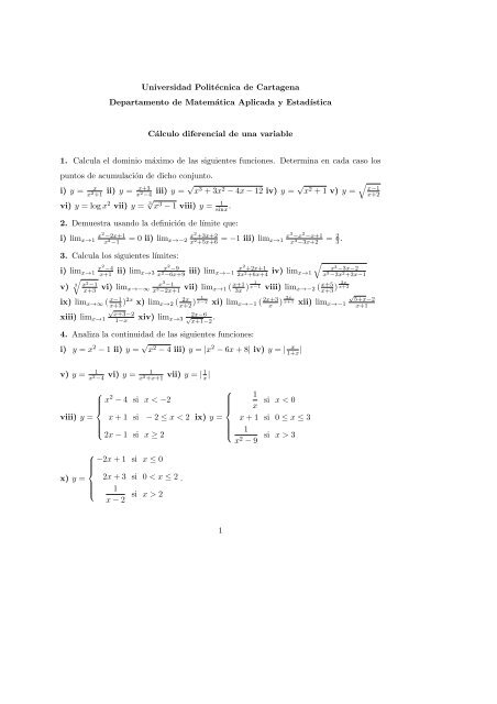
1. Calcula el dominio máximo de las siguientes funciones. Determina en cada caso los
puntos de acumulación de dicho conjunto.
i) y = x
x 2 +1
ii) y = x+3
x 2 −4 iii) y = √ x 3 + 3x 2 − 4x − 12 iv) y = √ x 2 + 1 v) y =
vi) y = log x 2 vii) y = 3√ x 3 − 1 viii) y = 1
sinx .
2. Demuestra usando la definición de límite que:
i) limx→1 x2 −2x+1
x 2 −1
3. Calcula los siguientes límites:
i) limx→1 x2 −4
v) 3
= 0 ii) limx→−2 x2 +3x+2
x2 +5x+6 = −1 iii) limx→1 x3−x 2 −x+1
x3−3x+2 x
x+1 ii) limx→3
2 −9
x2−6x+9 iii) limx→−1 x2 +2x+1
2x2 +6x+4
x2−1 x+3 vi) limx→−∞ x3−1 x3−2x+1 vii) limx→1 ( x+1
1
3x )
ix) limx→∞ ( x−1
xiii) limx→1
x+3 )2x x) limx→2 ( 2x
x+2
√
x+3−2
2x−6
1−x xiv) limx→3 √ .
x+1−2
1
) x−2 xi) limx→−1 ( 2x+3
4. Analiza la continuidad de las siguientes funciones:
iv) limx→1
x−1 viii) limx→−2 ( x+5
i) y = x 2 − 1 ii) y = √ x 2 − 4 iii) y = |x 2 − 6x + 8| iv) y = | x
1+x |
v) y = 1
x 2 −4
vi) y =
1
x 2 +x+1
vii) y = | 1
x |
⎧
x
⎪⎨
viii) y =
⎪⎩
2 − 4 si x < −2
x + 1 si − 2 ≤ x < 2
2x − 1 si x ≥ 2
⎧
−2x + 1 si x ≤ 0
⎪⎨
x) y = 2x + 3 si 0 < x ≤ 2 .
⎪⎩ 1
si x > 2
x − 2
⎧
⎪⎨
1
x
si x < 0
ix) y = x + 1 si 0 ≤ x ≤ 3
⎪⎩
1
x2 si x > 3
− 9
1
x
= 2
3 .
x 3 −3x−2
x 3 −3x 2 +3x−1
x+3
) 2x
x+2
) 2x
x+1 xii) limx→−1
x−1
x+2
√ 5+x−2
x+1

5. Determina a, b ∈ R para los⎧cuales las siguientes funciones son continuas:
ax − 5 si x ≤ −1
⎪⎨
i) f : R −→ R tal que f(x) = −ax + b si − 1 < x < 2
⎪⎩
−2ax + 3b si x ≥ 2
⎧
3x + a si
⎪⎨
− 2 ≤ x < −1
ii) g : [−2, 5[−→ R tal que g(x) = bx + a si − 1 ≤ x < 3
⎪⎩
2x − b si 3 ≤ x < 5
.
6. Demuestra, aplicando el Teorema de Bolzano que las siguientes ecuaciones tienen
solución en los intervalos indicados:
i) x 3 + 2x − 1 = 0 en ]0, 2[. ii) 1 − x = tanx en ]0, π/4[. iii) x = sinx en ] − π/6, π/6[.
iv) x n − 2 = 0 si n ∈ N, n > 1 en ]0, 2[.
7. Indica en cada apartado que hipótesis del Teorema de Bolzano falla y analiza si se
verifica o no la Tesis de dicho Teorema:
x − 1 si 0 ≤ x ≤ 1
i) f : [0, 2] −→ R | f(x) =
x 2 .
− 2 si 1 < x ≤ 2
ii) g : [1, 3] −→ R | g(x) = x 2 + 1.
8. Demuestra que todo polinomio de grado impar tiene por lo menos un raíz real.
9. Justifica que un hilo de alambre con forma circular calentado tiene dos puntos diame-
tralmente opuestos con la misma temperatura.
10. A partir de la definición de derivada, calcula:
i) f ′ (−1) siendo f(x) = x 2 − 5x + 6. ii) g ′ (2) siendo g(x) = x 2 + x + 1.
iii) j ′ (3) siendo j(x) = x+2
x+1 iv) l′ (−1) siendo l(x) = 1
x .
11. Calcula los puntos de la gráfica de la función f(x) cuya recta tangente en dichos
puntos forme un ángulo θ con la parte positiva del eje OX en los siguientes casos:
i) f(x) = x 2 − 4, θ = π
4 ii) y = sinx, recta tangente horizontal. iii) y = ex , θ = π
2 .
2

12. Analiza la continuidad y derivabilidad de las siguientes funciones:
i) f(x) =
x 2 si x ≤ 0
2x si x > 0
ii) f(x) =
2x + 5 si x ≤ −1
x 2 si x > −1
iii) f(x) =
x 2 − 5 si x < 2
3x − 7 si x ≥ 2
⎧
⎨ 1
si x < 0
iv) f(x) = x
⎩
2x 2 ⎧
⎧
⎨ |x|
si x = 0
⎨ |x + 1|
si x = 0
v) f(x) = x vi) f(x) = x
⎩
⎩
si x ≥ 0
1 si x = 0
1 si x = 0
vii) f(x) = |x+3| f(x) = |x2 ⎧
⎨ 1
si x = 0
−2x−3| viii) f(x) = |x|
⎩
1 si x = 0
13. Calcula la derivada de las siguientes funciones:
i) y = x−3
x+1
(x−1)2
ii) y = log x2 iii) y = sin 3 x2 iv) y = arctan3x−sinx 2
x
ix) f(x) = |x 2 −4|.
v) y = arcsin 2 ( x−1
x+2 )
vi) y = cos(cos(cosx)) vii) y = sec 2 x − cosecx 2 viii) y = 5 2sinx − x 4 ix) y = (x) x2
x) y = sinx x xi) y = (cosx) x xii) y = x arctan2 x .
14. Representa gráficamente las siguientes funciones:
i) y = x 3 − 6x 2 + 9x ii) y = −x 4 + x 2 iii) y = x2 −1
x iv) y = 1
x 2 +1
x vi) 1+|x| vii) y = log (x2 − 9) viii y = xe−x ix) y = sinx
x
v) y = x2
x 2 +x−4
x) y = sinxcosx.
15. Calcula las rectas tangentes a la gráfica de f(x) en sus puntos de inflexión en los
siguientes casos:
i) f(x) = 2x 3 − 3x 2 − 12x + 7 ii) f(x) = xe x iii) f(x) = x2
2
16. Demuestra las siguientes desigualdades:
i) tanx ≥ x si 0 ≤ x < π
2 ii) ex > 1
1+x
− logx.
si x > 0 iii) log x < x si x > 1.
17. Calcula las derivadas n-ésimas de las siguientes funciones:
i) y = log kx, k > 0 ii) y = cos kx, k > 0 iii) y = √ x iv) y = xe x .
18. Calcula entre todos los números positivos cuyo producto es 16, aquellos que tienen
suma mínima.
19. Calcula el punto de la parábola y = x 2 de menor distancia al punto P = (1, 2),
3

20. Calcula las dimensiones del triángulo isósceles de área máxima entre los que tienen
de perímetro 30 cm.
21. Calcula la distancia mínima del origen a la curva xy = 1.
22. Calcula las dimensiones del rectángulo de área máxima que tiene sus lados paralelos
a los ejes de coordenadas, inscrito en la elipse 4x 2 + y 2 = 1.
23. Calcula las dimensiones del rectángulo de área máxima inscrito en una circumferencia
de radio 8 cm.
24. Para cada una de las siguientes funciones, analiza si se verifican o no las hipótesis
del Teorema de Rolle. Si es posible, calcula un valor donde se obtenga la tesis.
i) y = x 2 − 4x + 2 en [1, 3]. ii) y = x 3 − 1 en [0, 1]. iii) y = |x − 1| en [0, 2].
25. Para cada una de las siguientes funciones, analiza si se verifican o no las hipótesis del
Teorema del valor medio de Lagrange. Si es posible, calcula un valor donde se obtenga
la tesis.
i) y = |x 2 − 9| en [1, 4]. ii) y = x 2 + 2 en [0, 2]. iii) y = x 2 + x + 1 en [−1, 1].
⎧
⎨ 1
iv) y = 2
⎩
x2 + x + 1 si x ≤ 0
x + 1 si x > 0
en [−1, 2].
26. Calcula los valores de a y b para los cuales las siguientes funciones satisfacen las
hipótesis del Teorema del valor medio de Lagrange en los intervalos indicados. Para
dichos valores, calcula un valor donde se obtenga la tesis.
i) f(x) =
ax 2 + bx + 1 si x ≤ 0
ax + b si x > 0
en [−1, 1]. ii) f(x) =
2x − a si x ≤ 1
ax + b si x > 1
en [−1, 2].
2
ax + 1 si x ≤ −1
2
ax + bx + 1 si x ≤ −1
iii) f(x) =
en [−4, 0]. iv) f(x) =
2x + b si x > −1
2
x − a si x < −1
ax + b si x > −1
2
ax − 1 si x ≤ 1
[−2, 0]. v) f(x) =
en [−2, 3]. vi) f(x) =
bx + 3 si x ≥ −1
2
−ax + 2b si x ≤ 1
2x + b si x > 1
[−1, 3]. vii) f(x) =
en [0, 4].
bx + a + 4 si x > 1
4
en
en

27. Dada la función f(x) = x 2 + 1, ¿Qué teorema afirma que existe x0 ∈] − 2, 1[ tal que
la recta tangente a la gráfica de f(x) en (x0, f(x0)) es paralela a la recta que pasa por
los puntos (−2, 5) y (1, 2). Calcula x0.
28. Analiza si f(x) y g(x) verifican las hipótesis del Teorema del valor medio de Cauchy
en los intervalos indicados. Si es posible, calcula un valor donde se obtenga la tesis.
i) f(x) = x 2 − 1, g(x) = x + 2 en [0, 3]. ii) f(x) = |x| y g(x) = x 2 − 3x + 1 en [1, 2].
iii) f(x) =
x 2 − 4 si x ≤ 2
x − 2 si x ≤ 2
y g(x) = x 2 + 2x + 1 en [0, 3].
29. Calcula los siguientes límites usando el Teorema de L’Hôpital:
i) limx→1 x3 −1
x 2 −1
ii) limx→0 1−cos ax
1−cos bx
v) lim x→0 + cosecx
log x vi) lim x→ π
2 +
ix) lim x→0 + tanx log x x) limx→0 ( 1
sinx
xiii) lim ex +cos x
e x +sinx
xiv) limx→ π
2
siendo a, b ∈ R. iii) limx→ π
4
1−tanx
x− π
4
iv) limx→0 sinx
x
secx
log(x− π
2 ) vii) limx→∞ xe−x viii) limx→0 ex−e sinx
x3 1 − x3 ) xi) limx→∞ x 1
x xii) limx→0 x−sinx
x3 (1 + 2 cos x) 1
cos x xv) limx→1
cos (x−1)−1
(log x) 2
xvi) lim x→0 + (cotanx) x xvii) limx→0 ( 1+tanx
1+sinx )cosecx xviii) limx→0 (cotanx − 1
x )
xix) limx→1
x
log x −
xxii) limx→0 e2x −cos 2 x 2
x 2 −senx
1
sin(x−1) xx) limx→∞ (cos 1
x )x xxi) limx→0 sen2x senx2 xxii) limx→0 tanx2
tan2x xxiv) limx→0
x cos(x+ π
2 )
log(1+x2 )+sin x2 xxv) limx→0 x2−sin 2 x
sinx2 30. Calcula el polinomio de Taylor de grado n de f(x) en x0 en los siguientes casos:
i) y = cos x, x0 = 1, n = 5.
ii) y = xsinx, x0 = 0, n = 6.
iii) y = tan2x, x0 = 0, n = 4.
iv) y = √ x, x0 = 1, n = 4.
v) y = log x, x = 1, n = 4.
vi) y = cosx, x = π
2 , n = 6.
31. Dada la función f(x) = √ 1 + x calcula:
i) Su polinomio de Mc. Laurin de grado 3.
ii) Aproxima √ 1.1 utilizando el polinomio obtenido en el apartado anterior y obtén la
menor posible de las cotas superiores del error cometido.
5
.

32. Dada la función f(x) = log x calcula:
i) Su polinomio de Taylor de grado 3 en x = 1.
ii) Aproxima log 0.9 utilizando el polinomio obtenido en el apartado anterior y obtén la
menor posible de las cotas superiores del error cometido.
33. Dada la función f(x) = √ x calcula:
i) Su polinomio de Taylor de grado 4 en x = 9.
ii) Aproxima √ 10 utilizando el polinomio obtenido en el apartado anterior y obtén la
menor posible de las cotas superiores del error cometido.
34. Obtén aproximaciones decimales con las cifras decimales exactas indicadas usando
el polinomio de Taylor adecuado:
i) 1
√1.1 con 3 decimales exactos.
ii) cos 0.1 con 3 cifras decimales exactas.
iii) e 0.1 con 4 cifras decimales exactas.
iv) √ 84 con 2 cifras decimales exactas.
v) e 0.1 sin0.1 con 3 cifras decimales exactas.
35. Usando el polinomio de Taylor de la función f(x) = 6arcsinx en x = 0, calcula una
aproximación de π con 4 cifras decimales. (Ayuda: π = f( 1
2 ))
36. Demostrar que |sinx − siny| ≤ |x − y| para todo x, y ∈ R.
37. Calcula el polinomio de Taylor de grado 3 de f(x) = e 2x en x = 0, aproxima el
valor de e 0.2 utilizando dicho polinomio y obtén una cota del error cometido con tal
aproximación.
38. Dada la función f(x) = e x calcula su polinomio de Taylor de grado 3 en x = 0,
aproxima 7√ e utilizando el polinomio calculado y obtén la menor posible de las cotas
superiores del error cometido.
39. Dada la función f(x) = sen(−2x), calcula su polinomio de Taylor de grado 3 en
x = 0, aproxima sen(−0.4) utilizando el polinomio calculado y obtén la menor posible de
las cotas superiores del error cometido.
6

40. Dada la función f(x) = cos(−2x), calcula su polinomio de Taylor de grado 2 en
x = 0, aproxima cos(−0.2) utilizando el polinomio calculado y obtén la menor posible de
las cotas superiores del error cometido.
41. Dada la función f(x) = √ x calcula su polinomio de Taylor de grado 2 en x = 81,
aproxima √ 80 utilizando el polinomio calculado y obtén la menor posible de las cotas
superiores del error cometido.
7