4. Integral de Riemann - DIM - Universidad de Chile
4. Integral de Riemann - DIM - Universidad de Chile
4. Integral de Riemann - DIM - Universidad de Chile

Create successful ePaper yourself
Turn your PDF publications into a flip-book with our unique Google optimized e-Paper software.
<strong>4.</strong> <strong>Integral</strong> <strong>de</strong> <strong>Riemann</strong><br />
<strong>4.</strong>1. Introducción<br />
Ingeniería Matemática<br />
FACULTAD DE CIENCIAS<br />
FÍSICAS Y MATEMÁTICAS<br />
UNIVERSIDAD DE CHILE<br />
Cálculo Diferencial e <strong>Integral</strong> 08-2<br />
Ingeniería Matemática<br />
<strong>Universidad</strong> <strong>de</strong> <strong>Chile</strong><br />
SEMANA 7: INTEGRAL DE RIEMANN<br />
La teoría <strong>de</strong> la integral <strong>de</strong> <strong>Riemann</strong> tiene un objetivo simple, que es: formalizar la<br />
noción <strong>de</strong> área mediante una <strong>de</strong>finición que sea compatible con las i<strong>de</strong>as comunes<br />
e intuitivas acerca <strong>de</strong> este concepto.<br />
Surge entonces la pregunta <strong>de</strong> ¿Cuales son estas i<strong>de</strong>as básicas?. Por ejemplo,<br />
una <strong>de</strong> ellas es que el área <strong>de</strong> una superficie cuadrada <strong>de</strong> lado a sea a 2 . Si esto<br />
es verda<strong>de</strong>ro, se <strong>de</strong>be concluir que la superficie <strong>de</strong> un rectángulo <strong>de</strong> lados a y b<br />
es a · b.<br />
<strong>4.</strong>2. Condiciones básicas para una <strong>de</strong>finición <strong>de</strong> área<br />
Sea E un conjunto <strong>de</strong> puntos en el plano OXY . El área <strong>de</strong>l conjunto E será un<br />
número real A(E) que cumple las siguientes condiciones.<br />
(A1) A(E) ≥ 0<br />
(A2) E ⊆ F =⇒ A(E) ≤ A(F)<br />
(A3) Si E ∩ F = ∅ =⇒ A(E ∪ F) = A(E) + A(F)<br />
(A4) El área <strong>de</strong> una región rectangular E <strong>de</strong> lados a y b es A(E) = a · b<br />
Estas 4 condiciones son necesarias y suficientes para tener una buena <strong>de</strong>finición<br />
<strong>de</strong> área. Se verá mas a<strong>de</strong>lante, en el transcurso <strong>de</strong>l curso, que la integral <strong>de</strong><br />
<strong>Riemann</strong> las satisface a<strong>de</strong>cuadamente.<br />
Observación: Las cuatro propieda<strong>de</strong>s elementales anteriores no son in<strong>de</strong>pendientes<br />
entre sí, ya que por ejemplo (A2) es una consecuencia <strong>de</strong> (A1) y (A3)<br />
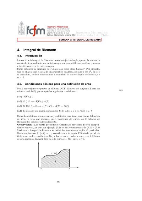
Mediante la integral <strong>de</strong> <strong>Riemann</strong> se <strong>de</strong>finirá el área <strong>de</strong> una región E particular:<br />
Dada una función f : [a,b] → + consi<strong>de</strong>remos la región R limitada por el eje<br />
OX, la curva <strong>de</strong> ecuación y = f(x) y las rectas verticales x = a y x = b. El área<br />
<strong>de</strong> esta región se llamará área bajo la curva y = f(x) entre a y b.<br />
00000000000<br />
11111111111<br />
00000000000<br />
11111111111<br />
00000000000<br />
11111111111<br />
y=f(x)<br />
00000000000<br />
11111111111<br />
00000000000<br />
11111111111<br />
00000000000<br />
11111111111<br />
00000000000<br />
11111111111<br />
00000000000<br />
11111111111<br />
00000000000<br />
11111111111<br />
R<br />
00000000000<br />
11111111111<br />
00000000000<br />
11111111111<br />
00000000000<br />
11111111111<br />
00000000000<br />
11111111111<br />
00000000000<br />
11111111111<br />
a b<br />
66<br />
área
Ingeniería Matemática<br />
<strong>Universidad</strong> <strong>de</strong> <strong>Chile</strong><br />
Mediante un ejemplo se mostrará un método para <strong>de</strong>terminar el área bajo una<br />
curva, que nos indicará el procedimiento a seguir en la <strong>de</strong>finición <strong>de</strong> la integral<br />
<strong>de</strong> <strong>Riemann</strong>.<br />
Ejemplo<br />
Dada la función f(x) = x 2 , se <strong>de</strong>sea calcular el área encerrada entre x = 0 y<br />
x = b > 0 bajo la curva y = f(x).<br />
Etapa 1.<br />
000000000000<br />
111111111111<br />
000000000000<br />
111111111111<br />
000000000000<br />
111111111111<br />
000000000000<br />
111111111111<br />
000000000000<br />
111111111111<br />
000000000000<br />
111111111111<br />
000000000000<br />
111111111111<br />
000000000000<br />
111111111111<br />
000000000000<br />
111111111111<br />
000000000000<br />
111111111111<br />
y=x<br />
000000000000<br />
111111111111<br />
000000000000<br />
111111111111<br />
000000000000<br />
111111111111<br />
000000000000<br />
111111111111<br />
000000000000<br />
111111111111<br />
000000000000<br />
111111111111<br />
2<br />
a b<br />
Dividiremos el intervalo [0,b] en n partes iguales don<strong>de</strong> cada una <strong>de</strong> estas partes<br />
tiene longitud h = b<br />
n . Si llamamos xi a los puntos <strong>de</strong> la división, se tiene que:<br />
xi = i(b/n).<br />
De este modo se ha dividido el intervalo [0,b] en n sub-intervalos Ii = [xi−1,xi]<br />
<strong>de</strong> longitud h cada uno.<br />
Etapa 2.<br />
En cada intervalo Ii se levanta el rectángulo inscrito al sector parabólico<br />
<strong>de</strong> mayor altura posible. Este i-ésimo rectángulo inscrito posee las<br />
siguientes propieda<strong>de</strong>s:<br />
base = h<br />
altura = f(xi−1)<br />
área = h · f(xi−1)<br />
= b<br />
n ·<br />
<br />
(i − 1) b<br />
n<br />
2<br />
67<br />
=<br />
3 b<br />
(i − 1)<br />
n<br />
2<br />
y=x 2<br />
00 11<br />
00 11<br />
00 11<br />
00 11<br />
00 11<br />
a xi-1 xi<br />
b
Etapa 3.<br />
y=x 2<br />
00 11<br />
00 11<br />
00 11<br />
00 11<br />
00 11<br />
00 11<br />
00 11<br />
00 11<br />
00 11<br />
00 11<br />
i-1 i<br />
a x x b<br />
Etapa <strong>4.</strong><br />
Ingeniería Matemática<br />
<strong>Universidad</strong> <strong>de</strong> <strong>Chile</strong><br />
De igual forma en cada intervalo Ii se levanta el rectángulo circunscrito<br />
al sector parabólico <strong>de</strong> menor altura posible. Este i-ésimo<br />
rectángulo circunscrito posee las siguientes propieda<strong>de</strong>s:<br />
base = h<br />
altura = f(xi)<br />
área = h · f(xi)<br />
= b<br />
n ·<br />
<br />
i b<br />
n<br />
Con esta construcción, se ve fácilmente que el área A que se <strong>de</strong>sea calcular<br />
está acotada <strong>de</strong>l modo siguiente<br />
n<br />
i=1<br />
( b<br />
n )3 (i − 1) 2 ≤ A ≤<br />
n<br />
i=1<br />
( b<br />
n )3 i 2 .<br />
Las sumatorias anteriores se calculan fácilmente recordando que<br />
De este modo,<br />
n<br />
i 2 =<br />
i=1<br />
n(n + 1)(2n + 1)<br />
.<br />
6<br />
n<br />
(i − 1) 2 n−1 <br />
= i 2 n−1 <br />
= i 2 =<br />
i=1<br />
i=0<br />
i=1<br />
Así las cotas para el área A buscada son<br />
(n − 1)n(2n − 1)<br />
.<br />
6<br />
b3 (n + 1)(2n − 1)<br />
6 n2 ≤ A ≤ b3 (n + 1)(2n + 1)<br />
6 n2 La <strong>de</strong>sigualdad anterior es válida ∀n ∈ , luego, olvidando el significado geométrico<br />
<strong>de</strong> los números que allá intervienen, se pue<strong>de</strong> pensar en una <strong>de</strong>sigualdad <strong>de</strong><br />
sucesiones reales. Por lo tanto, si tomamos el límite cuando n → ∞ queda:<br />
b 3<br />
3<br />
≤ A ≤ b3<br />
3 ,<br />
<strong>de</strong> don<strong>de</strong> se <strong>de</strong>duce que el área buscada es<br />
A = b3<br />
3 .<br />
68<br />
2<br />
=<br />
3 b<br />
i<br />
n<br />
2<br />
◭ Ejercicio
Ingeniería Matemática<br />
<strong>Universidad</strong> <strong>de</strong> <strong>Chile</strong><br />
Ejercicio <strong>4.</strong>1: Del mismo modo como se ha resuelto este ejercicio, se propone<br />
al lector calcular las áreas encerradas bajo las funciones f(x) = 1,<br />
f(x) = x y f(x) = x 3 . Por cierto en los dos primeros casos los resultados<br />
son bien conocidos, no así en el tercero. Nótese que al resolver estos ejercicios<br />
se observa lo siguiente:<br />
función Area entre 0 y b don<strong>de</strong><br />
f(x) = x0 b · h h = 1<br />
1 f(x) = x<br />
2 f(x) = x<br />
b·h<br />
2<br />
b·h<br />
3<br />
h = b<br />
h = b2 3 f(x) = x b·h h = b3 Se <strong>de</strong>ja también al lector la tarea <strong>de</strong> formular una generalización a estos<br />
resultados a potencias superiores.<br />
69<br />
4
Ingeniería Matemática<br />
<strong>Universidad</strong> <strong>de</strong> <strong>Chile</strong><br />
Ejercicio <strong>4.</strong>2: Como último ejercicio propuesto se plantea calcular el área<br />
encerrada bajo la función sen(x) entre 0 y π/2.<br />
Después <strong>de</strong> estos ejercicios <strong>de</strong> motivación po<strong>de</strong>mos comenzar a <strong>de</strong>finir el concepto<br />
<strong>de</strong> integral <strong>de</strong> <strong>Riemann</strong> <strong>de</strong> una función.<br />
<strong>4.</strong>3. Definiciones<br />
◭ Ejercicio<br />
Definición <strong>4.</strong>1 (Partición <strong>de</strong> un intervalo). Partición<br />
El conjunto P = {x0,x1,...,xn} es una partición <strong>de</strong>l intervalo [a,b] si a = x0 < P = {x0, x1, ..., xn}<br />
x1 < x2 < · · · < xn = b.<br />
Si P es una partición <strong>de</strong> [a,b], se llama norma <strong>de</strong> P y se <strong>de</strong>nota por |P | al real:<br />
|P | = máx{(xi − xi−1) : i = 1,...,n}<br />
Definición <strong>4.</strong>2 (Sumas Superiores e Inferiores). sumas superiores e<br />
inferiores<br />
Sea f una función <strong>de</strong>finida y acotada en [a,b] 1 . Sea P = {x0,x1,...,xn} una<br />
partición <strong>de</strong> [a,b]. Como f es acotada en [a,b], también lo es en cada intervalo<br />
Ii = [xi−1,xi] ∀i = 1,...,n, luego po<strong>de</strong>mos <strong>de</strong>finir:<br />
mi(f) = ínf{f(x) : x ∈ [xi−1,xi]}<br />
Mi(f) = sup{f(x) : x ∈ [xi−1,xi]}<br />
(La existencia <strong>de</strong> mi(f) y Mi(f) está garantizada por ser f acotada en [xi−1,xi]).<br />
Con esto se <strong>de</strong>finen las sumas siguientes:<br />
1) S(f,P) = n<br />
Mi(f)(xi − xi−1) se llama suma superior <strong>de</strong> f correspondiente<br />
i=1<br />
a la partición P<br />
2) s(f,P) = n<br />
i=1<br />
la partición P.<br />
Interpretación Geométrica<br />
mi(f)(xi −xi−1) se llama suma inferior <strong>de</strong> f correspondiente a<br />
Si f(x) ≥ 0 ∀x ∈ [a,b], entonces las sumas superior e inferior <strong>de</strong> f tienen una<br />
interpretación geométrica sencilla. s(f,P) correspon<strong>de</strong> al área <strong>de</strong> los rectángulos<br />
inscritos. S(f,P) es el área <strong>de</strong> los rectángulos circunscritos.<br />
1 Que f sea una función <strong>de</strong>finida y acotada en [a, b] significa que [a, b] ⊆ Dom(f), es <strong>de</strong>cir<br />
f(x) existe ∀x ∈ [a, b] y a<strong>de</strong>más existen las constantes m y M tales que:<br />
m = ínf{f(x) : x ∈ [a, b]}<br />
M = sup{f(x) : x ∈ [a, b]}<br />
70
Propiedad Importante.<br />
Ingeniería Matemática<br />
<strong>Universidad</strong> <strong>de</strong> <strong>Chile</strong><br />
Sea f una función acotada y <strong>de</strong>finida en [a,b]. Sea P = {x0,...,xn} una partición<br />
<strong>de</strong> [a,b], cualquiera. Sean<br />
m = ínf{f(x) : x ∈ [a,b]}<br />
M = sup{f(x) : x ∈ [a,b]}<br />
mi(f) = ínf{f(x) : x ∈ [xi−1,xi]}<br />
Mi(f) = sup{f(x) : x ∈ [xi−1,xi]}<br />
es claro que ∀i = 1,...,n se tiene que: m, M, mi(f), Mi(f)<br />
Luego:<br />
m ≤ mi(f) ≤ Mi(f) ≤ M.<br />
∀i ∈ {1,...,n} m(xi−xi−1) ≤ mi(f)(xi−xi−1) ≤ Mi(f)(xi−xi−1) ≤ M(xi−xi−1).<br />
Sumando <strong>de</strong>s<strong>de</strong> i = 1 hasta i = n se obtiene que:<br />
m(b − a) ≤ s(f,P) ≤ S(f,P) ≤ M(b − a). (<strong>4.</strong>1)<br />
Como P es una partición cualquiera, se concluye que el conjunto <strong>de</strong> las sumas<br />
inferiores <strong>de</strong> f es acotado, así como el conjunto <strong>de</strong> las sumas superiores <strong>de</strong> f.<br />
Esta propiedad da lugar a las dos <strong>de</strong>finiciones siguientes:<br />
Definición <strong>4.</strong>3 (<strong>Integral</strong>es Superiores e Inferiores). integrales superiores e<br />
inferiores<br />
Sea P [a,b] el conjunto <strong>de</strong> todas las particiones <strong>de</strong> [a,b]. Sea f una función <strong>de</strong>finida<br />
y acotada sobre [a,b]. Los números reales<br />
b<br />
a<br />
b<br />
a<br />
f = sup <br />
s(f,P) : P ∈ P [a,b] , y<br />
f = ínf <br />
S(f,P) : P ∈ P [a,b] ,<br />
se llaman integral inferior <strong>de</strong> f en [a,b] e integral superior <strong>de</strong> f en [a,b], respectivamente.<br />
Observación: Por la propiedad <strong>de</strong>mostrada anteriormente, se sabe que el conjunto<br />
<strong>de</strong> las sumas inferiores era acotado, lo mismo que el conjunto <strong>de</strong> las sumas<br />
superiores, luego en virtud <strong>de</strong>l Axioma <strong>de</strong>l supremo, están garantizadas las existencias<br />
<strong>de</strong> b b<br />
f y <strong>de</strong> f. Para que todo esto sea válido es necesario y suficiente,<br />
a a<br />
que f este <strong>de</strong>finida en [a,b] y sea acotada en dicho intervalo.<br />
Definición <strong>4.</strong>4 (Refinamiento <strong>de</strong> una partición o partición más fina).<br />
Sean P y Q dos particiones <strong>de</strong> [a,b], si P ⊆ Q, diremos que Q es un refinamiento<br />
P o una partición más fina que P.<br />
71<br />
b b<br />
f,<br />
a af refinamiento
Ingeniería Matemática<br />
<strong>Universidad</strong> <strong>de</strong> <strong>Chile</strong><br />
Ejemplo <strong>4.</strong>1.<br />
Si P1 y P2 son 2 particiones cualesquiera <strong>de</strong> [a,b], entonces P = P1 ∪ P2 es<br />
un refinamiento <strong>de</strong> P1 y <strong>de</strong> P2.<br />
Proposición <strong>4.</strong>1. Si P ⊆ Q entonces<br />
s(f,P) ≤ s(f,Q), y<br />
S(f,P) ≥ S(f,Q)<br />
Demostración. Si P = Q, la proposición es trivialmente cierta. Por lo tanto<br />
en el resto <strong>de</strong> la <strong>de</strong>mostración trataremos el caso en que P = Q.<br />
Para fijar i<strong>de</strong>as digamos que P = {x0,...,xn}, sea ¯x el primer punto que aparece<br />
en Q y no en P, entonces hay un k ∈ {1,...,n} tal que xk−1 < ¯x < xk.<br />
Sea P1 = {x0,...,xk−1, ¯x,xk,...,xn} y sean<br />
Claramente:<br />
m ′ (f) = ínf{f(x) : x ∈ [xk−1, ¯x]} y<br />
m ′′ (f) = ínf{f(x) : x ∈ [¯x,xk]}.<br />
mk(f) ≤ m ′ (f) y mk(f) ≤ m ′′ (f).<br />
Con esto calculemos las sumas inferiores <strong>de</strong> f para las particiones P y P1:<br />
s(f,P) =<br />
≤<br />
Por lo tanto<br />
n<br />
mi(f)(∆xi)<br />
i=1<br />
<br />
k−1<br />
mi(f)(∆xi) + m ′ (f)(¯x − xk−1) + m ′′ (f)(xk − ¯x) +<br />
i=1<br />
= s(f,P1).<br />
s(f,P) ≤ s(f,P1).<br />
n<br />
i=k+1<br />
mi(f)∆xi<br />
Repitiendo este procedimiento un número finito <strong>de</strong> veces obtenemos que: s(f,P) ≤<br />
s(f,Q).<br />
La <strong>de</strong>sigualdad con sumas superiores se <strong>de</strong>muestra en forma análoga y se <strong>de</strong>ja<br />
propuesta como un ejercicio.<br />
Observación: Como a<strong>de</strong>más s(f,Q) ≤ S(f,Q), se concluye que ∀P,Q ∈ P [a,b].<br />
P ⊆ Q =⇒ s(f,P) ≤ s(f,Q) ≤ S(f,Q) ≤ S(f,P).<br />
Entonces, si P1 y P2 son particiones <strong>de</strong> [a,b], tomando la partición P = P1 ∪ P2<br />
que es un refinamiento <strong>de</strong> P1 y P2, se tiene que<br />
s(f,P1) ≤ s(f,P) ≤ S(f,P) ≤ S(f,P2),<br />
72
es <strong>de</strong>cir,<br />
s(f,P1) ≤ S(f,P2) ∀P1,P2 ∈ P [a,b].<br />
Ingeniería Matemática<br />
<strong>Universidad</strong> <strong>de</strong> <strong>Chile</strong><br />
O sea cualquier suma inferior es cota inferior <strong>de</strong>l conjunto <strong>de</strong> sumas superiores<br />
y recíprocamente.<br />
Proposición <strong>4.</strong>2. Si f está <strong>de</strong>finida y acotada en [a,b], y m ≤ f(x) ≤ M<br />
∀x ∈ [a,b], entonces<br />
m(b − a) ≤<br />
b<br />
a<br />
f ≤<br />
b<br />
a<br />
f ≤ M(b − a)<br />
Demostración. Primeramente, como m(b−a) es una cota inferior <strong>de</strong> <br />
s(f,P) : P ∈ P [a,b] ,<br />
(Ecuación <strong>4.</strong>1 en página 71) y como b<br />
a f = sup <br />
s(f,P) : P ∈ P [a,b] , resulta que<br />
Análogamente:<br />
b<br />
f ≤ M(b − a).<br />
m(b − a) ≤<br />
a<br />
Para probar la <strong>de</strong>sigualdad central, consi<strong>de</strong>remos dos particiones P1 y P2 cua-<br />
lesquiera <strong>de</strong> [a,b]. Como s(f,P1) ≤ S(f,P2) entonces, fijando P1, se tiene que<br />
s(f,P1) es una cota inferior <strong>de</strong>l conjunto <br />
S(f,P) : P ∈ P [a,b] y por lo tanto:<br />
b<br />
s(f,P1) ≤ ínf <br />
S(f,P) : P ∈ P [a,b] =<br />
La <strong>de</strong>sigualdad anterior se cumple ∀P1 ∈ P [a,b] luego el numero<br />
superior <strong>de</strong>l conjunto <br />
s(f,P) : P ∈ P [a,b] y por lo tanto:<br />
b<br />
a<br />
a<br />
f.<br />
f ≥ sup <br />
s(f,P) : P ∈ P [a,b] =<br />
Esta ultima expresión prueba la proposición.<br />
b<br />
b<br />
a<br />
a<br />
f<br />
f.<br />
b<br />
a<br />
f es una cota<br />
Definición <strong>4.</strong>5. Diremos que una función f <strong>de</strong>finida y acotada en [a,b] es integrable<br />
según <strong>Riemann</strong> si se cumple que b b<br />
f = f. En tal caso, el valor común <strong>Riemann</strong> integrable<br />
a a<br />
<strong>de</strong> estas dos integrales se llama simplemente la integral <strong>de</strong> f en [a,b] y se <strong>de</strong>nota<br />
b<br />
b<br />
por f.<br />
f<br />
a<br />
Teorema <strong>4.</strong>1 (Condición <strong>de</strong> <strong>Riemann</strong>). Una función f <strong>de</strong>finida y acotada<br />
en un intervalo [a,b] es <strong>Riemann</strong>-integrable en [a,b] ssi:<br />
(∀ǫ > 0)(∃P ∈ P [a,b]) S(f,P) − s(f,P) < ǫ<br />
73<br />
a
Ingeniería Matemática<br />
<strong>Universidad</strong> <strong>de</strong> <strong>Chile</strong><br />
Demostración. Probemos primeramente que la condición <strong>de</strong> <strong>Riemann</strong> es suficiente,<br />
es <strong>de</strong>cir, si la condición <strong>de</strong> <strong>Riemann</strong> se cumple entonces la función es<br />
integrable.<br />
Sea ǫ > 0. Sabemos que<br />
Pero<br />
entonces,<br />
0 ≤<br />
(∃P ∈ P [a,b]) S(f,P) − s(f,P) < ǫ.<br />
b<br />
a<br />
−<br />
f −<br />
b<br />
a<br />
b<br />
a<br />
b<br />
a<br />
f ≤ S(f,P)<br />
f ≤ −s(f,P)<br />
f ≤ S(f,P) − s(f,P) < ǫ.<br />
Como esta ultima <strong>de</strong>sigualdad es válida ∀ǫ > 0 se concluye que b b<br />
f = f y<br />
a a<br />
por lo tanto f es integrable en [a,b].<br />
Probemos ahora que la condición <strong>de</strong> <strong>Riemann</strong> es necesaria, es <strong>de</strong>cir, que si f es<br />
integrable entonces la condición <strong>de</strong> <strong>Riemann</strong> <strong>de</strong>be cumplirse.<br />
Sabemos que<br />
b<br />
a<br />
f = inf <br />
S(f,P) : P ∈ P [a,b]<br />
= sup <br />
s(f,P) : P ∈ P [a,b]<br />
entonces, dado ǫ > 0, en virtud <strong>de</strong> la caracterización ǫ <strong>de</strong>l supremo y <strong>de</strong>l ínfimo<br />
<strong>de</strong> un conjunto po<strong>de</strong>mos garantizar la existencia <strong>de</strong> particiones P1,P2 <strong>de</strong> [a,b]<br />
tales que<br />
s(f,P1) ><br />
S(f,P2) <<br />
b<br />
a<br />
b<br />
a<br />
f − ǫ<br />
2<br />
f + ǫ<br />
2<br />
Si a<strong>de</strong>más consi<strong>de</strong>ramos la partición P = P1 ∪ P2, (refinamiento <strong>de</strong> P1 y <strong>de</strong> P2)<br />
y recordando que las sumas inferiores crecen y las superiores <strong>de</strong>crecen al tomar<br />
refinamientos, se <strong>de</strong>duce que<br />
s(f,P) ><br />
S(f,P) <<br />
74<br />
b<br />
a<br />
b<br />
a<br />
f − ǫ<br />
2<br />
f + ǫ<br />
2
y por lo tanto<br />
es <strong>de</strong>cir<br />
S(f,P) − ǫ ǫ<br />
< s(f,P) +<br />
2 2<br />
S(f,P) − s(f,P) < ǫ.<br />
Ingeniería Matemática<br />
<strong>Universidad</strong> <strong>de</strong> <strong>Chile</strong><br />
Con esto, dado ǫ > 0 arbitrario, hemos encontrado una partición que verifica la<br />
condición <strong>de</strong> <strong>Riemann</strong>. <br />
Ejemplo <strong>4.</strong>2.<br />
Probar que f(x) = 1<br />
x es integrable en [1,2].<br />
Si P = {x0,...,xn} es una partición <strong>de</strong> [1,2] entonces en cada intervalo Ii se<br />
. Por lo tanto,<br />
tiene que: mi(f) = 1<br />
xi y Mi(f) = 1<br />
xi−1<br />
S(f,P) =<br />
s(f,P) =<br />
n<br />
i=1<br />
n<br />
i=1<br />
( xi − xi−1<br />
xi−1<br />
( xi − xi−1<br />
xi<br />
Notemos que esta sumas no son fáciles <strong>de</strong> calcular para una partición arbitraria.<br />
Sin embargo lo único que se <strong>de</strong>sea aquí, es probar que la función es<br />
integrable y no calcular la integral. Con este objetivo en mente, nos basta con<br />
verificar la condición <strong>de</strong> <strong>Riemann</strong>. Calculemos entonces la diferencia entre las<br />
dos sumas:<br />
S(f,P) − s(f,P) =<br />
Como las variables xi ∈ [1,2] entonces<br />
=<br />
n<br />
i=1<br />
( 1<br />
xi−1<br />
) y<br />
).<br />
n (xi − xi−1) 2<br />
.<br />
i=1<br />
− 1<br />
)(xi − xi−1)<br />
xi<br />
xixi−1<br />
1 1<br />
< < 1,<br />
2 xi<br />
y por lo tanto po<strong>de</strong>mos acotar la diferencia como<br />
n<br />
S(f,P) − s(f,P) ≤ (xi − xi−1) 2 .<br />
Para terminar recordamos que<br />
i=1<br />
xi − xi−1 < |P |,<br />
don<strong>de</strong> |P | es la norma <strong>de</strong> la partición P. Entonces<br />
S(f,P) − s(f,P) < |P | · (2 − 1) = |P |.<br />
En consecuencia para satisfacer la condición <strong>de</strong> <strong>Riemann</strong>, dado ǫ > 0 basta<br />
consi<strong>de</strong>rar una partición P ∈ P [1,2] con norma |P | ≤ ǫ. Es <strong>de</strong>cir<br />
Por lo tanto, f(x) = 1<br />
x<br />
|P | ≤ ǫ =⇒ S(f,P) − s(f,P) < ǫ.<br />
es integrable en [1,2].<br />
75
Ejemplo <strong>4.</strong>3. <br />
1 si x ∈<br />
Probar que f(x) =<br />
0 si x ∈ I<br />
no es integrable en [0,1].<br />
Ingeniería Matemática<br />
<strong>Universidad</strong> <strong>de</strong> <strong>Chile</strong><br />
Sea P = {x0,...,xn} una partición <strong>de</strong> [0,1], claramente en cada intervalo<br />
Ii = [xi−1,xi] se tiene que<br />
mi(f) = 0, y<br />
Mi(f) = 1.<br />
Por lo tanto las sumas <strong>de</strong> <strong>Riemann</strong> son<br />
S(f,P) =<br />
=<br />
s(f,P) =<br />
Claramente se cumple que<br />
n<br />
Mi(f)(xi − xi−1)<br />
i=1<br />
n<br />
xi − xi−1 = b − a = 1, y<br />
i=1<br />
n<br />
mi(f)(xi − xi−1) = 0.<br />
i=1<br />
S(f,P) − s(f,P) = 1 ∀P ∈ P [0,1]<br />
y luego la condición <strong>de</strong> <strong>Riemann</strong> no se cumple. Por lo tanto f no es integrable<br />
en [0,1].<br />
Observación: Este último ejemplo muestra que una función pue<strong>de</strong> estar <strong>de</strong>finida<br />
y ser acotada en un intervalo y sin embargo no ser <strong>Riemann</strong> integrable. Es<br />
<strong>de</strong>cir ser <strong>Riemann</strong> integrable es una propiedad mas fuerte o exigente que sólo<br />
ser <strong>de</strong>finida y acotada.<br />
En este ejemplo también se pue<strong>de</strong> observar que<br />
b<br />
a<br />
1<br />
0<br />
f(x) = 0, y<br />
f(x) = 1.<br />
<strong>4.</strong><strong>4.</strong> Estudio <strong>de</strong> Funciones Integrables<br />
En esta sección nos preocupamos <strong>de</strong> saber bajo que requisitos se pue<strong>de</strong> garantizar<br />
que una función <strong>de</strong>finida y acotada en un intervalo es <strong>Riemann</strong> integrable. Los<br />
resultados más importantes en este sentido son el teorema (<strong>4.</strong>2) que garantiza<br />
que las funciones continuas son integrables y la proposición <strong>4.</strong>3 que hace lo propio<br />
con las funciones monótonas.<br />
A<strong>de</strong>más se verá que en este tipo <strong>de</strong> funciones (las continuas o monótonas) la<br />
condición <strong>de</strong> <strong>Riemann</strong> se cumple en la medida que la norma <strong>de</strong> la partición<br />
sea suficientemente pequeña. Esto último permite enten<strong>de</strong>r la integral como el<br />
76
Ingeniería Matemática<br />
<strong>Universidad</strong> <strong>de</strong> <strong>Chile</strong><br />
límite <strong>de</strong> las sumas inferiores o superiores cuando la norma <strong>de</strong> la partición tien<strong>de</strong><br />
a cero.<br />
Proposición <strong>4.</strong>3. Si f es una función <strong>de</strong>finida, acotada y monótona en [a,b],<br />
entonces es integrable en [a,b].<br />
Demostración. Supongamos que se trata <strong>de</strong> una función creciente (la <strong>de</strong>mostración<br />
en el caso <strong>de</strong> función <strong>de</strong>creciente se propone como ejercicio). Si<br />
P = {x0,...,xn} es una partición <strong>de</strong> [a,b] entonces<br />
y entonces<br />
S(f,P) =<br />
s(f,P) =<br />
S(f,P) − s(f,P) =<br />
≤<br />
n<br />
f(xi)∆xi<br />
i=1<br />
n<br />
f(xi−1)∆xi<br />
i=1<br />
n<br />
[f(xi) − f(xi−1)] ∆xi<br />
i=1<br />
n<br />
[f(xi) − f(xi−1)] |P |<br />
i=1<br />
= |P |[f(b) − f(a)] .<br />
Por lo tanto, dado ǫ > 0 arbitrario, es fácil encontrar particiones con norma |P | ≤<br />
2 con lo cual la condición <strong>de</strong> <strong>Riemann</strong> se cumple satisfactoriamente.<br />
1<br />
f(b)−f(a)+1<br />
Teorema <strong>4.</strong>2. Si f es una función continua en [a,b] entonces es integrable en<br />
[a,b]<br />
Demostración. Es bien sabido que las funciones continuas en un intervalo<br />
cerrado y acotado [a,b] son uniformemente continuas, es <strong>de</strong>cir satisfacen la propiedad<br />
∀ǫ > 0, ∃δ > 0, ∀x1,x2 ∈ [a,b], |x1 − x2| ≤ δ =⇒ |f(x1) − f(x2)| ≤ ǫ .<br />
Con esta proposición no es difícil probar la condición <strong>de</strong> <strong>Riemann</strong>. En efecto,<br />
dado ǫ > 0 arbitrario, la proposición anterior garantiza la existencia <strong>de</strong> δ > 0<br />
tal que si |x1 − x2| ≤ δ entonces<br />
|f(x1) − f(x2)| ≤ ǫ<br />
. (<strong>4.</strong>2)<br />
b − a<br />
2 El 1 en el <strong>de</strong>nominador f(b) − f(a) + 1 se introduce solo para evitar dividir por cero (en<br />
el caso <strong>de</strong> una función constante).<br />
77
Ingeniería Matemática<br />
<strong>Universidad</strong> <strong>de</strong> <strong>Chile</strong><br />
Consi<strong>de</strong>remos una partición P ∈ P [a,b] con norma |P | ≤ δ. Como f es continua<br />
en [a,b], también lo será en cada uno <strong>de</strong> los intervalos Ii = [xi−1,xi] <strong>de</strong>finidos<br />
por la partición y por lo tanto el supremo Mi y el ínfimo mi en dicho intervalo<br />
serán alcanzados como imágenes <strong>de</strong> algún punto. Es <strong>de</strong>cir,<br />
Luego<br />
Pero como |x ′ i<br />
|f(x ′′<br />
i ) − f(x′ i<br />
∃x ′ i ∈ [xi−1,xi], f(x ′ i) = ínf {f(x) : x ∈ [xi−1,xi]}<br />
∃x ′′<br />
i ∈ [xi−1,xi], f(x ′′<br />
i ) = sup {f(x) : x ∈ [xi−1,xi]} .<br />
S(f,P) − s(f,P) =<br />
n<br />
i=1<br />
[f(x ′′<br />
i ) − f(x ′ i)] ∆xi.<br />
− x′′<br />
i | ≤ ∆xi ≤ |P | ≤ δ entonces se cumple (<strong>4.</strong>2), es <strong>de</strong>cir que<br />
)| ≤ ǫ<br />
b−a<br />
. En consecuencia<br />
S(f,P) − s(f,P) ≤<br />
ǫ<br />
b − a<br />
= ǫ.<br />
n<br />
i=1<br />
∆xi.<br />
Notemos que en la <strong>de</strong>mostración anterior solo se requiere que |P | ≤ δ. Esto<br />
permite concluir el siguiente corolario.<br />
Corolario <strong>4.</strong>1. Si f es continua en [a,b] Entonces:<br />
<br />
n<br />
<br />
(∀ǫ > 0)(∃δ > 0)(∀P ∈ P [a,b]) |P | ≤ δ ⇒ f(¯xi)(xi − xi−1) −<br />
<br />
i=1<br />
b<br />
a<br />
<br />
<br />
<br />
f<br />
≤ ǫ ,<br />
<br />
don<strong>de</strong> los valores ¯xi son números arbitrarios en el correspondiente i − ésimo<br />
intervalo [xi−1,xi] <strong>de</strong>finido por la partición P. (por ejemplo ¯xi = xi−1+xi<br />
2 )<br />
Demostración. El teorema anterior dice que<br />
(∀ǫ > 0)(∃δ > 0)(∀P ∈ P [a,b]) {|P | ≤ δ ⇒ S(f,P) − s(f,P) ≤ ǫ} .<br />
A<strong>de</strong>más, si P = {x0,...,xn} es una <strong>de</strong> las particiones anteriores y ¯xi ∈ [xi−1,xi]<br />
entonces<br />
mi(f) ≤ f(¯xi) ≤ Mi(f).<br />
multiplicando por ∆xi y sumando <strong>de</strong> i = 1 hasta i = n se obtiene<br />
n<br />
s(f,P) ≤ f(¯xi)(xi − xi−1) ≤ S(f,P). (<strong>4.</strong>3)<br />
i=1<br />
Por otro lado como la función es integrable se sabe que<br />
s(f,P) ≤<br />
b<br />
a<br />
f ≤ S(f,P). (<strong>4.</strong>4)<br />
Las <strong>de</strong>sigualda<strong>de</strong>s (<strong>4.</strong>3) y (<strong>4.</strong>4) se interpretan como que los números n i=1 f(¯xi)(xi−<br />
xi−1) y b<br />
f pertenecen a un mismo intervalo <strong>de</strong> largo no mayor que ǫ. Por lo<br />
a<br />
tanto, <br />
n<br />
<br />
b <br />
<br />
f(¯xi)(xi − xi−1) − f<br />
≤ ǫ<br />
<br />
i=1<br />
78<br />
a
Ingeniería Matemática<br />
<strong>Universidad</strong> <strong>de</strong> <strong>Chile</strong><br />
Observación: El corolario anterior se pue<strong>de</strong> interpretar como una noción <strong>de</strong><br />
límite cuando |P | → 0, es <strong>de</strong>cir, po<strong>de</strong>mos escribir que cuando una función es<br />
continua su integral es<br />
b<br />
a<br />
f = lím<br />
|P |→0<br />
i=1<br />
n<br />
f(¯xi)∆xi.<br />
La expresión anterior motiva la siguiente notación, <strong>de</strong>nominada notación <strong>de</strong><br />
Leibnitz para integrales<br />
b<br />
a<br />
f =<br />
b<br />
a<br />
f(x)dx.<br />
Observación: Si f es continua en [a,b] también se cumple que<br />
<br />
<br />
b <br />
<br />
(∀ǫ > 0)(∃δ > 0)(∀P ∈ P [a,b]) |P | < δ ⇒ S(f,P)<br />
− f<br />
< ǫ<br />
<br />
y que<br />
<br />
<br />
<br />
(∀ǫ > 0)(∃δ > 0)(∀P ∈ P [a,b]) |P | < δ ⇒ s(f,P)<br />
−<br />
<br />
a<br />
b<br />
a<br />
<br />
<br />
<br />
f<br />
< ǫ .<br />
<br />
Observación: El corolario y la observación (<strong>4.</strong>4) también se cumple si f<br />
monótona.<br />
Luego: si f es continua en [a,b] o bien monótona en [a,b] entonces se pue<strong>de</strong> <strong>de</strong>cir<br />
que:<br />
b<br />
a<br />
f = lím s(f,P) = lím S(f,P) = lím<br />
|P |→0 |P |→0 |P |→0<br />
<strong>4.</strong>5. Propieda<strong>de</strong>s <strong>de</strong> la <strong>Integral</strong><br />
n<br />
f(¯xi)∆xi.<br />
Ya hemos visto cual es la <strong>de</strong>finición <strong>de</strong> la integral <strong>de</strong> una función. Sabemos que<br />
se trata <strong>de</strong> un número real asociado a la función. Sabemos que este real existe<br />
para un conjunto <strong>de</strong> funciones llamadas las funciones <strong>Riemann</strong> integrables, entre<br />
las cuales se encuentran las funciones continuas y las funciones monótonas. En<br />
cuanto al cálculo <strong>de</strong> integrales sólo conocemos la <strong>de</strong>finición y sabemos que en<br />
la medida que las normas <strong>de</strong> las particiones sean pequeñas, las integrales se<br />
aproximan por sumatorias llamadas las sumas <strong>de</strong> <strong>Riemann</strong>. En esta sección nos<br />
interesa estudiar algunas propieda<strong>de</strong>s <strong>de</strong>l operador integral. Los resultados más<br />
atractivos se resumen en el Teorema <strong>4.</strong>3 que dice que este operador es lineal y<br />
monótono. También veremos cómo se pue<strong>de</strong> exten<strong>de</strong>r la noción <strong>de</strong> integral a los<br />
casos a = b y a > b.<br />
<strong>4.</strong>5.1. Lemas Previos (Propieda<strong>de</strong>s Básicas)<br />
Comenzamos por enunciar algunos lemas previos relativos a las integrales inferiores<br />
y superiores.<br />
Lema 1. Si f es una función integrable en [a,b], a < b, y [r,s] ⊆ [a,b], con<br />
r < s, entonces f es integrable en [r,s].<br />
79<br />
i=1<br />
b<br />
a f(x)dx
Ingeniería Matemática<br />
<strong>Universidad</strong> <strong>de</strong> <strong>Chile</strong><br />
Lema 2. Si f está <strong>de</strong>finida y es acotada en [a,b], a < b, y c ∈ (a,b) entonces<br />
b<br />
a<br />
b<br />
a<br />
f ≥<br />
f ≤<br />
c<br />
a<br />
c<br />
a<br />
f +<br />
f +<br />
b<br />
c<br />
b<br />
c<br />
f (<strong>4.</strong>5)<br />
f (<strong>4.</strong>6)<br />
Lema 3. Si f y g son dos funciones <strong>de</strong>finidas y acotadas en [a,b], a < b, entonces:<br />
b<br />
a<br />
b<br />
f +<br />
a<br />
b<br />
a<br />
g ≤<br />
(f + g) ≤<br />
b<br />
a<br />
b<br />
a<br />
(f + g) (<strong>4.</strong>7)<br />
f +<br />
b<br />
a<br />
g (<strong>4.</strong>8)<br />
Demostración. (<strong>de</strong>l lema 1) Como f es integrable en [a,b] ⇒ se cumple la<br />
condición <strong>de</strong> <strong>Riemann</strong> en [a,b], es <strong>de</strong>cir:<br />
(∀ǫ > 0)(∃P ∈ P [a,b]) S(f,P) − s(f,P) ≤ ǫ.<br />
Sea Q = P ∪{r,s}, es claro que como r y s ∈ [a,b], entonces Q es un refinamiento<br />
<strong>de</strong> P, luego S(f,Q) − s(f,Q) ≤ ǫ.<br />
Para fijar i<strong>de</strong>as, digamos que Q = {x0,x1,...,xn} y que r = xk,s = xℓ con<br />
0 ≤ k < ℓ ≤ n.<br />
Sea entonces Q ′ = {xk,xk+1, · · · ,xℓ} = Q ∩ [r,s]. Es claro que Q ′ resulta ser<br />
una partición <strong>de</strong> [r,s] tal que:<br />
S(f,Q ′ )−s(f,Q ′ ) =<br />
ℓ<br />
i=k+1<br />
(Mi−mi)∆xi ≤<br />
n<br />
(Mi−mi)∆xi = s(f,Q)−s(f,Q) < ǫ.<br />
Luego la partición Q ′ muestra que f verifica la condición <strong>de</strong> <strong>Riemann</strong> y por lo<br />
tanto es una función integrable en [r,s].<br />
Demostración. (<strong>de</strong>l Lema 2)<br />
Para <strong>de</strong>mostrar (<strong>4.</strong>5) sean P1 ∈ P [a,c] y P2 ∈ P [c,b] dos particiones arbitrarias <strong>de</strong><br />
[a,c] y [c,b] respectivamente. Formemos la partición P <strong>de</strong> [a,b] como P = P1∪P2.<br />
Claramente<br />
i=1<br />
s(f,P1) + s(f,P2) = s(f,P) ≤<br />
Esta <strong>de</strong>sigualdad se pue<strong>de</strong> escribir así<br />
s(f,P1) ≤<br />
b<br />
a<br />
b<br />
a<br />
f.<br />
f − s(f,P2) ∀P1 ∈ P [a,c].<br />
En consecuencia el real <strong>de</strong> la <strong>de</strong>recha es cota superior <strong>de</strong>l conjunto <strong>de</strong> sumas<br />
inferiores <strong>de</strong> f en [a,c] y por lo tanto<br />
b<br />
a<br />
f − s(f,P2) ≥<br />
80<br />
c<br />
a<br />
f.
Esta expresión se pue<strong>de</strong> también escribir así<br />
b<br />
a<br />
f −<br />
c<br />
a<br />
f ≥ s(f,P2) ∀P2 ∈ P [c,b],<br />
Ingeniería Matemática<br />
<strong>Universidad</strong> <strong>de</strong> <strong>Chile</strong><br />
es <strong>de</strong>cir el número <strong>de</strong> la izquierda es una cota superior <strong>de</strong>l conjunto <strong>de</strong> sumas<br />
inferiores <strong>de</strong> f en [c,b]. Entonces este número es mayor o igual al supremo, es<br />
<strong>de</strong>cir b c b<br />
f − f ≥ f.<br />
La <strong>de</strong>mostración <strong>de</strong> (<strong>4.</strong>6) es análoga y se <strong>de</strong>ja como ejercicio.<br />
a<br />
a<br />
Demostración. (<strong>de</strong>l lema 3)<br />
Como en el caso anterior, sólo <strong>de</strong>mostraremos la fórmula (<strong>4.</strong>7), y <strong>de</strong>jaremos (<strong>4.</strong>8)<br />
como ejercicio. Para probar esta fórmula sean P1 y P2 particiones cualesquiera<br />
<strong>de</strong> [a,b] y sea P = P1 ∪ P2. Claramente<br />
c<br />
s(f,P1) + s(g,P2) ≤ s(f,P) + s(g,P). (<strong>4.</strong>9)<br />
Para fijar i<strong>de</strong>as digamos que P = {x0,...,xn} entonces<br />
s(f,P) =<br />
s(g,P) =<br />
s(f + g,P) =<br />
n<br />
mi(f)∆xi<br />
i=1<br />
n<br />
mi(g)∆xi<br />
i=1<br />
n<br />
mi(f + g)∆xi.<br />
i=1<br />
Recor<strong>de</strong>mos que ∀x ∈ Ii,mi(f) ≤ f(x) ∧ mi(g) ≤ g(x) luego mi(f) + mi(g) ≤<br />
mi(f + g) y entonces<br />
s(f,P) + s(g,P) ≤ s(f + g,P) ≤<br />
b<br />
a<br />
(f + g). (<strong>4.</strong>10)<br />
En la última <strong>de</strong>sigualdad hemos recordado que la integral inferior es una cota<br />
superior <strong>de</strong>l conjunto <strong>de</strong> sumas inferiores <strong>de</strong> una función (aquí la f + g).<br />
Combinando las ecuaciones (<strong>4.</strong>9) y (<strong>4.</strong>10) se tiene que<br />
s(f,P1) + s(g,P2) ≤<br />
b<br />
a<br />
(f + g).<br />
Como esta <strong>de</strong>sigualdad es válida ∀P1,P2 ∈ P [a,b] entonces <strong>de</strong><br />
se <strong>de</strong>duce que<br />
s(f,P1) ≤<br />
b<br />
a<br />
f ≤<br />
b<br />
b<br />
a<br />
a<br />
(f + g) − s(g.P2)<br />
(f + g) − s(g.P2),<br />
81
y luego <strong>de</strong><br />
se <strong>de</strong>duce que<br />
s(g,P2) ≤<br />
b<br />
a<br />
g ≤<br />
es <strong>de</strong>cir b<br />
f +<br />
a<br />
b<br />
b<br />
a<br />
b<br />
a<br />
a<br />
(f + g) −<br />
(f + g) −<br />
g ≤<br />
b<br />
a<br />
b<br />
b<br />
a<br />
a<br />
f,<br />
(f + g).<br />
<strong>4.</strong>5.2. Teorema con las propieda<strong>de</strong>s <strong>de</strong> la integral<br />
f<br />
Ingeniería Matemática<br />
<strong>Universidad</strong> <strong>de</strong> <strong>Chile</strong><br />
Usando los lemas probados en la subsección prece<strong>de</strong>nte se pue<strong>de</strong> <strong>de</strong>mostrar el<br />
siguiente teorema que resume las propieda<strong>de</strong>s más importantes <strong>de</strong> la integral.<br />
Teorema <strong>4.</strong>3 (Propieda<strong>de</strong>s <strong>de</strong> la <strong>Integral</strong>).<br />
1. Si c ∈ , entonces b<br />
c = c(b − a)<br />
a<br />
2. Si f es integrable en [a,b] y c ∈ (a,b), entonces f es integrable en [a,c] y<br />
[c,b], y a<strong>de</strong>más<br />
b<br />
a<br />
f =<br />
c<br />
3. Si f es integrable en [a,c], y en [c,b], entonces f es integrable en [a,b] y<br />
b<br />
a<br />
f =<br />
a<br />
c<br />
<strong>4.</strong> Si f y g son funciones integrables en [a,b] entonces (f + g) es integrable<br />
en [a,b] y<br />
b<br />
a<br />
a<br />
(f + g) =<br />
5. Si f es una función integrable en [a,b] y α ∈ entonces (αf) es integrable<br />
en [a,b] y<br />
b<br />
a<br />
f +<br />
f +<br />
b<br />
a<br />
(αf) = α<br />
b<br />
c<br />
b<br />
c<br />
f +<br />
6. Si f y g son integrables en [a,b] y f(x) ≤ g(x) ∀x ∈ [a,b] entonces<br />
b<br />
a<br />
f ≤<br />
7. Si f es integrable en [a,b], entonces |f| es integrable en [a,b] y<br />
<br />
<br />
<br />
b <br />
<br />
f<br />
≤<br />
b<br />
|f|<br />
a<br />
82<br />
b<br />
a<br />
a<br />
b<br />
a<br />
g<br />
f<br />
f<br />
f<br />
b<br />
a<br />
g
Ingeniería Matemática<br />
<strong>Universidad</strong> <strong>de</strong> <strong>Chile</strong><br />
Demostración. 1. Sea f(x) = c ∀x ∈ [a,b], sea P = {x0,...,xn} una<br />
partición cualquiera <strong>de</strong> [a,b] entonces en cada intervalo [xi−1,xi] se cumple<br />
que<br />
mi(f) = Mi(f) = c<br />
por lo tanto las sumas inferior y superior son<br />
Claramente entonces<br />
Luego,<br />
s(f,p) = S(f,P) = c ∆xi = c(b − a).<br />
b<br />
a<br />
f =<br />
b<br />
a<br />
f = c(b − a) ⇒<br />
b<br />
a<br />
b<br />
a<br />
c = c(b − a).<br />
c = c(b − a)<br />
2. Por lema 1, si f es integrable en [a,b] y c ∈ [a,b], entonces f es integrable<br />
en [a,c] y [c,b] (ambos ⊆ [a,b]) a<strong>de</strong>más por lema 2:<br />
b<br />
a<br />
f ≤<br />
c<br />
<strong>de</strong> don<strong>de</strong> claramente b<br />
f =<br />
a<br />
a<br />
f +<br />
c<br />
3. Si f es integrable en [a,c] y [c,b], entonces está <strong>de</strong>finida y acotada en [a,b].<br />
Por lema 2:<br />
b<br />
a<br />
f ≤<br />
c<br />
a<br />
a<br />
f +<br />
b<br />
c<br />
f +<br />
b<br />
c<br />
f ≤<br />
b<br />
c<br />
f ≤<br />
Pero como la <strong>de</strong>sigualdad contraria siempre es cierta, se <strong>de</strong>duce que f es<br />
integrable en [a,b] y su integral vale<br />
b<br />
a<br />
f =<br />
c<br />
a<br />
f +<br />
<strong>4.</strong> Como f y g son integrables en [a,b] entonces el lema 3 se escribe así:<br />
b<br />
a<br />
(f + g) ≤<br />
b<br />
a<br />
f +<br />
Luego (f + g) es integrable en [a,b] y<br />
b<br />
a<br />
(f + g) ≤<br />
b<br />
a<br />
f +<br />
83<br />
b<br />
a<br />
b<br />
a<br />
b<br />
c<br />
g ≤<br />
g ≤<br />
b<br />
f.<br />
a<br />
b<br />
f.<br />
a<br />
b<br />
a<br />
b<br />
a<br />
f<br />
f.<br />
(f + g).<br />
(f + g).
Ingeniería Matemática<br />
<strong>Universidad</strong> <strong>de</strong> <strong>Chile</strong><br />
5. Sea P = {x0,...,xn} una partición cualquiera <strong>de</strong> [a,b]. Analicemos primeramente<br />
el caso α ≥ 0. En este caso se tiene que<br />
Por lo tanto<br />
Con lo cual<br />
es <strong>de</strong>cir<br />
mi(αf) = αmi(f), y<br />
Mi(αf) = αMi(f).<br />
S(αf,P) = αS(f,P), y<br />
s(αf,P) = αs(f,P).<br />
sup{s(αf,P)} = sup{αs(f,P)} = α sup{s(f,P)}, y<br />
ínf{S(αf,P)} = ínf{αS(f,P)} = α ínf{S(f,P)},<br />
b<br />
a<br />
αf =<br />
b<br />
por lo tanto αf es integrable en [a,b] y<br />
a<br />
αf = α<br />
b<br />
a<br />
b<br />
a<br />
f<br />
αf = α<br />
En las líneas anteriores se ha usado el resultado bien conocido que dice<br />
que si α ≥ 0 y A ⊆ es un conjunto acotado entonces<br />
sup(αA) = α sup(A), y<br />
ínf(αA) = α ínf(A).<br />
b<br />
En el caso en que α < 0 la propiedad anterior se cambia por<br />
por lo tanto ahora tendremos que<br />
<strong>de</strong> don<strong>de</strong><br />
con lo cual<br />
es <strong>de</strong>cir<br />
sup(αA) = α ínf(A), y<br />
ínf(αA) = α sup(A),<br />
mi(αf) = αMi(f), y Mi(αf) = αmi(f)<br />
S(αf,P) = αs(f,P), y s(αf,P) = αS(f,P)<br />
sup{s(αf,P)} = sup{αS(f,P)} = α ínf{S(f,p)}, y<br />
ínf{S(αf,P)} = ínf{αs(f,P)} = α sup{s(f,p)},<br />
b<br />
a<br />
αf =<br />
b<br />
Por lo tanto αf es integrable en [a,b] y<br />
84<br />
a<br />
αf = α<br />
b<br />
a<br />
b<br />
a<br />
f.<br />
αf = α<br />
a<br />
b<br />
a<br />
f.<br />
f.
Ingeniería Matemática<br />
<strong>Universidad</strong> <strong>de</strong> <strong>Chile</strong><br />
6. Sea h = g − f. Como f(x) ≤ g(x)∀x ∈ [a,b] entonces h(x) ≥ 0∀x ∈ [a,b].<br />
A<strong>de</strong>más h = g +(−1)f es integrable en [a,b] y<br />
b<br />
a<br />
h =<br />
b<br />
a<br />
g −<br />
b<br />
a<br />
f. Como<br />
h(x) ≥ 0∀x ∈ [a,b], entonces para cualquier partición <strong>de</strong> [a,b] se tendrá que<br />
mi(h) ≥ 0 luego s(h,P) ≥ 0.<br />
Entonces<br />
0 ≤ s(h,P) ≤<br />
b<br />
a<br />
h =<br />
<strong>de</strong> don<strong>de</strong> b<br />
f ≤<br />
7. Sean<br />
y<br />
f + (x) =<br />
f − <br />
(x) =<br />
a<br />
b<br />
a<br />
b<br />
a<br />
h =<br />
g.<br />
b<br />
a<br />
g −<br />
f(x) si f(x) ≥ 0<br />
0 si f(x) < 0<br />
b<br />
0 si f(x) ≥ 0<br />
−f(x) si f(x) < 0 .<br />
Entonces f = f + − f − y |f| = f + + f − . Para probar que |f| es integrable<br />
probaremos previamente que f + lo es. Si P = {x0,...,xn} es una partición<br />
cualquiera <strong>de</strong> [a,b] entonces como f(x) ≤ f + (x), ∀x ∈ [a,b] entonces<br />
mi(f) ≤ mi(f + ), o sea,<br />
−mi(f + ) ≤ −mi(f). (<strong>4.</strong>11)<br />
A<strong>de</strong>más, si Mi(f) ≥ 0 entonces Mi(f + ) = Mi(f) y entonces sumando con<br />
(<strong>4.</strong>11) se obtiene que<br />
Mi(f + ) − mi(f + ) ≤ Mi(f) − mi(f).<br />
Si por el contrario Mi(f) < 0 entonces f será negativa en el intervalo y<br />
luego f + = 0. Por lo tanto Mi(f + ) = mi(f + ) = 0 <strong>de</strong> don<strong>de</strong> claramente<br />
Mi(f + ) − mi(f + ) = 0 ≤ Mi(f) − mi(f).<br />
En <strong>de</strong>finitiva, en cualquier intervalo <strong>de</strong> la partición se cumple que<br />
Mi(f + ) − mi(f + ) ≤ Mi(f) − mi(f) ∀i = 1,...,n<br />
y por lo tanto sumando<br />
S(f + ,P) − s(f + ,P) ≤ S(f,P) − s(f,P).<br />
Gracias a esta última <strong>de</strong>sigualdad, <strong>de</strong>ducimos que ya que f es integrable<br />
en [a,b], entonces (∀ǫ > 0)(∃P ′ ∈ P [a,b]) tal que<br />
S(f,P ′ ) − s(f,P ′ ) ≤ ǫ<br />
85<br />
a<br />
f,
y por lo tanto<br />
luego f + es integrable en [a,b].<br />
S(f + ,P ′ ) − s(f + ,P ′ ) ≤ ǫ,<br />
Ingeniería Matemática<br />
<strong>Universidad</strong> <strong>de</strong> <strong>Chile</strong><br />
Como f = f + − f − entonces f − = f + − f y en consecuencia f − también<br />
es integrable. Por último como |f| = f + + f − es la suma <strong>de</strong> funciones<br />
integrables, entonces también es integrable en [a,b].<br />
Para <strong>de</strong>mostrar la <strong>de</strong>sigualdad basta con recordar que<br />
y en consecuencia<br />
−|f(x)| ≤ f(x) ≤ |f(x)| ∀x ∈ [a,b]<br />
−<br />
b<br />
es <strong>de</strong>cir, <br />
<strong>4.</strong>5.3. <strong>Integral</strong> <strong>de</strong> a a b con a ≥ b<br />
a<br />
|f| ≤<br />
b<br />
a<br />
b<br />
a<br />
<br />
<br />
<br />
f<br />
≤<br />
Definición <strong>4.</strong>6. Sea f una función integrable en un intervalo [p,q]. Si a,b ∈<br />
[p,q] son tales que a ≥ b entonces se <strong>de</strong>fine la integral <strong>de</strong> a a b <strong>de</strong>l modo siguiente:<br />
b<br />
a<br />
b<br />
a<br />
f = −<br />
a<br />
b<br />
f ≤<br />
b<br />
a<br />
f = 0 si a = b.<br />
b<br />
|f|<br />
a<br />
|f|,<br />
f si a > b, o<br />
con esta <strong>de</strong>finición, las propieda<strong>de</strong>s <strong>de</strong> la integral se pue<strong>de</strong>n enunciar así:<br />
Proposición <strong>4.</strong><strong>4.</strong> Sean f y g integrales en [p,q] y a,b ∈ [p,q] entonces:<br />
1)<br />
2)<br />
3)<br />
b<br />
a b<br />
a b<br />
a b<br />
α = α(b − a), ∀α ∈<br />
f =<br />
c<br />
a<br />
αf = α<br />
f +<br />
b<br />
a<br />
b<br />
b<br />
c<br />
f, ∀c ∈ [p,q]<br />
f, ∀α ∈<br />
b<br />
4) (f + g) = f + g<br />
a<br />
a a <br />
<br />
5) 0 ≤ f(x) ≤ g(x), ∀x ∈ [p,q] ⇒ b<br />
a f<br />
<br />
<br />
≤ b<br />
a g<br />
<br />
<br />
<br />
<br />
<br />
6) b<br />
a f<br />
<br />
<br />
≤ b<br />
a |f|<br />
<br />
<br />
<br />
Demostración. La <strong>de</strong>mostraciones son sencillas y se <strong>de</strong>jan propuestas como<br />
ejercicios. ◭ Ejercicio<br />
86