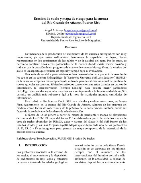
Erosión de suelo y mapa de riesgo para la cuenca del Río Grande ...

Erosión de suelo y mapa de riesgo para la cuenca
del Río Grande de Añasco, Puerto Rico
Ángel A. Anaya (angel.a.anaya@gmail.com)
Edwin J. Colón (edwinjcolon@gmail.com)
Departamento de Ingeniería Civil
Universidad de Puerto Rico Recinto de Mayagüez.
Resumen
Estimaciones de la producción de sedimentos de las cuencas hidrográficas son muy
importantes, ya que estos sedimentos disminuyen la capacidad de lagos, tienen
repercusiones en los ecosistemas de las bahías y de la calidad del agua. Por lo tanto, es
necesario localizar éstas áreas potenciales de la cuenca donde existe mayor erosión y
trabajar con la creación de un programa de manejo de cuencas hidrográficas. La erosión del
suelo es un aspecto que requiere de capital y tiempo para su evaluación.
Una serie de modelos paramétricos se han desarrollado para predecir la erosión de
los suelos en las cuencas hidrográficas, la “Reviewed Universal Soil Loss Equation” (RUSLE)
es la ecuación empírica más ampliamente utilizada para la estimación anual de pérdida de
suelos agrícolas en cuencas. Si bien los métodos convencionales están basados en puntos de
información, la teleobservación (Remote Sensing) hace posible medir parámetros
hidrológicos en escalas espaciales mayores, esta ventaja unida a la funcionalidad de un SIG
permite un análisis más robusto y ágil a la hora de manipular grandes cantidades de
información.
Este trabajo utiliza la ecuación RUSLE para calcular y evaluar estas zonas, en Puerto
Rico, básicamente, en la cuenca del Río Grande de Añasco. Algunos de los insumos del
modelo, como factor de cobertura y de la práctica de la conservación también puede ser
factor de éxito derivado de los datos de teleobservación.
El factor de LS se generó a partir de mapas de pendiente y mapas de elevaciones
derivados de los DEM. El mapa del factor K fue elaborado a partir de la de los mapas de
usos de suelos obtenidos de SURGO, datos y valores del factor K del Soil Survey de los
Estados Unidos y las Islas Vírgenes (1998). Mapas que cubren cada uno de los parámetros
(R, K, LS, C y P) se integraron para generar un mapa compuesto de la intensidad de la
erosión sobre la cuenca.
Palabras clave: Teleobservación, RUSLE, GIS, Erosión De Suelos.
I. INTRODUCCIÓN
Los problemas asociados a la erosión de
los suelos, el movimiento y la deposición
de sedimentos en ríos, lagos y estuarios
persisten a través de las edades geológicas
en casi todas las partes de la tierra. Pero la
situación se ve agravada en los últimos
tiempos con el aumento de las
intervenciones del hombre con el medio
ambiente. En la actualidad, la calidad de
los datos disponibles es extremadamente
1

variada. La planificación del uso de tierras
basada en datos poco fiables puede
conducir a graves y costosos errores. La
erosión del suelo es una investigación
intensidad de capital y tiempo.
Extrapolación global sobre la base de
datos generados por diversos y no
estandarizados métodos pueden dar lugar
a grandes errores y también puede
conducir a errores costosos y crítica sobre
cuestiones de política. En este estudio, la
funcionalidad de los GIS se utiliza
extensamente en la preparación del mapa
de la erosión. La cuenca del Rio Grande de
Añasco está influenciada por el hombre y
el desarrollo de la erosión del suelo y el
transporte de sedimentos al lago
disminución de su capacidad. La
teleobservación proporciona una
conveniente solución para este problema.
Además, el volumen de datos recogidos
con la ayuda de técnicas de
teleobservación son mejor manejados y
utilizados con la ayuda de los Sistemas de
Información Geográfica (GIS).
II.
OBJETIVOS DEL ESTUDIO
• Cuantificar la cantidad de
sedimento generado en la cuenca del
Río Grande de Añasco, correlacionar
estos valores con los datos históricos
y los patrones de sedimentación
actual en la bahía.
• Generar un mapa de riesgo de
erodabilidad a partir de
clasificaciones de los diferentes
parámetros que controlan la física de
este fenómeno.
III.
METODOLOGÍA
La pérdida de suelo se define como la
cantidad de suelo perdido en un plazo de
tiempo determinado, en una superficie
de la tierra que ha sufrido la pérdida de
suelo neto. Se expresa en unidades de
masa por unidad de área (Ton ha ‐ 1 y ‐ 1 )
Este documento utiliza la Ecuación
Universal de Pérdida de Suelos Revisada
(RUSLE) La RUSLE puede expresarse de
la siguiente manera:
A = R*K*LS*C*P (1)
Donde A es el calculado la pérdida de
suelo por unidad de superficie, expresada
en las unidades seleccionadas para K y el
período seleccionado para R.
(R) = Erosividad de la lluvia
(K) = Susceptibilidad de erosión del suelo
(L) = Largo de la pendiente
(S) = Magnitud de la pendiente
(C) = Cubierta y manejo de cultivos
(P) = residuos prácticas de conservación
(A) = Pérdida de suelos promedio por el
período de tiempo representado por R,
generalmente un año.
Figura 1 . Metodología
2

Figura 1, muestra un esquema sobre la
metodología utilizada en este trabajo.
Incluye los diferentes componentes de
obtener y calcular para el último cálculo
de la erosión del suelo en Rio Grande de
Arecibo.
IV.
ÁREA DEL STUDIO
El Rio Grande de Añasco y su cuenca se
encuentra en la costa occidental de
Puerto Rico entre las latitudes 18 ° 20'N y
18 ° 05'N y las longitudes 67 ° 15'W y 66 °
45'W.
El Río Grande de Añasco se origina cerca
de la Cordillera Central, corrientes al
oeste, y desemboca en la Bahía de
Añasco. Tiene su origen de la unión del
Río Blanco y el Río Prieto en el límite del
Barrio Espino y Pesuela del municipio de
Lares. Cruza por los municipios de
Adjuntas, Lares, Las Marías, San
Sebastián, Añasco, Mayagüez. Tiene una
longitud aproximada de 40 millas (64
kilómetros) desde su origen hasta que
desemboca en el Pasaje de Mona al oeste
de Puerto Rico. Tiene de 20 a 60 pies de
ancho y de 2 a 20 pies de profundidad.
La parte alta de la cuenca contienen
cuatro embalses conectados por tuberías;
El Lago Toro, Lago Prieto, Lago Guayo, y
el Lago Yahuecas. El valle aluvial del Río
Grande de Añasco cubre un área de
aproximadamente 18 mi 2 . La cuenca es
delimitada por colinas al norte, este y
sur, y por la Bahía de Añasco, al oeste.
Las dos zonas montañosas lo son las
Cadena de San Francisco, y las montañas
Atalaya al norte, y las Colinas de Uroyán
al sureste. Los afluentes del Río Grande
de Añasco que desembocan aguas abajo
en el l valle son el Río Dagüey y el Río
Cañas. El Caño La Puente y Caño
Boquilla son más pequeños arroyos que
atraviesan el valle.
Figura 2. Mapa de localización y elevación del
área de estudio
Las elevaciones dentro de la cuenca
varían desde el valle aluvial con 30
metros sobre el nivel medio del mar
hasta su mayor altitud que se encuentra
en las montañas situadas en la región en
la Cordillera Central, con el Monte
Guilarte a 3953 metros de altura sobre el
nivel medio del mar.
V. FACTORES PARA LA
ECUACIÓN (RUSLE)
1200
1150
1100
1050
1000
950
900
850
800
750
700
650
600
550
500
450
400
350
300
250
200
150
100
50
0
FACTOR R
Para calcular esta parámetro se utilizo
la formula de Arnoldus, en función de la
precipitación promedio mensual y anual.
3

R= 0.0302 * RI 1.9 (Arnoldus 1980) (2)
Se utilizaron ocho estaciones de lluvia
a usar para generar mapas de
precipitación media mensual y anual
mediante el uso de algoritmos
geostadísticos como Kriggging y la
función de base radial. (figura 3)
ESTACION
ADJUNTAS 1
NW
ADJUNTAS
SUBSTATION
LARES
LO
N
18
10'
18
10'
18
16'
LA
T ESTE NORTE R
66
43' 741491.9 2009931 832.6867
66
48' 732672.9 2009823 765.1255
66
50' 729014.5 2020852 1005.821
FACTOR K
El factor susceptibilidad de erosión del
suelo, es la tasa de pérdida de suelos por
unidad EI para un suelo específico.
Se preparó a partir del mapa de uso de
suelo de la cuenca, obtenido de SSURGO.
Figura 5. (K) susceptibilidad de erosión del
suelo con unidades de Ton*ha*hr*ha ‐1 *MJ*mm ‐1
0.3
0.28
0.26
0.24
0.22
0.2
0.18
0.16
0.14
0.12
0.1
0.08
0.06
0.04
0.02
0
MAYAGUEZ
CITY
MAYAGUEZ
AIRPORT
18
10'
18
15'
67
07' 699164.4 2009451 734.657
67
09' 695544.3 2018639 682.112
FACTOR LS
Para construir el mapa raster de este
factor para la cuenca se procederá de la
siguiente forma:
PUERTO
REAL
SAN
SEBASTIAN 2
WNW
18
04'
18
21'
67
10' 693984.2 1998329 319.2235
67
01' 709525.3 2029856 1027.094
• Se calculó el mapa de pendientes a
partir del mdt.
• Se calculó el mapa LS a partir de la
metodología propuesta por SURGO
UTUADO
18
16'
66
40' 746642.5 2021069 638.485
Figura 3. Estaciones del USGS
Figura 4. (R) Erosividad por lluvia con
unidades de MJ*ha ‐1 *mm*hr ‐1
950
900
850
800
750
700
650
600
550
500
450
400
350
300
250
200
150
100
50
0
LS = f(L, S) (3)
Uso de la DEM (Digital Elevation Model)
con 30 metros de resolución espacial
para la zona de estudio, el factor de L * S
se calculó utilizando:
LS = L/22*(0.065+0.045*S+0.0065*S 2 )
(4)
L = longitud (metros) fija a 30 metros.
S = pendiente (radianes).
4

El mapa del factor de LS fue creado a
partir de los DEM y el cálculo de
pendientes, primero en la obtención de
la red en cada píxel un valor de LS.
Figura 6. (LS) Características de las pendientes
del suelo con unidades de Ton*ha ‐1 *yr ‐1
FACTOR C
El factor cubierta y manejo, es
función del tipo de vegetación, Para
calcular este parámetro se usaran
imágenes satelitales, de sensores MSS,
TM y ETM, a resolución de pixel de 30
metros, y con una ventana temporal de
desde los 70’s hasta imágenes
posteriores al 2000.
20
19
18
17
16
15
14
13
12
11
10
9
8
7
6
5
4
3
2
1
0
Figura 8 . Imagen color verdadero del sensor
TM
Figura 9. Imagen color verdadero del sensor
ETM+
Aplicando una clasificación no
supervisada del tipo K medios utilizando
el programa ENVI 4.3 con 8 clases y 5
iteraciones se obtuvo los siguientes
resultados (figura , , )
Se comenzó creando un “subset” de las
imágenes del “Path”: 005 y “Row”: 047
para que solo incluyera el área deseada
para el estudio. (figuras 7, 8, 9 )
Figura 10. Kmeans de la imagen del MSS
Figura 7. Imagen color falso del sensor MSS
Figura 11 . Kmeans de la imagen del TM
5

Figura 12 . Kmeans de la imagen del ETM+
CATEGORIA
Cuerpos de agua 0
Bosque Denso 0.002
Bosque Medio 0.006
Grama 0.12
Cultivos 0.1
Ciudad 0
Figura 13 .Valores utilizados para C por clase.
Combinando estos valores con el
resultado de la clasificación del K medios
y la máscara de la cuenca se producen los
mapas del factor C para las tres
imágenes. (figuras 14, 15, 16)
MSS
Figura 14 . (C) Cubierta y manejo de cultivos
MSS
C
0.115
0.11
0.105
0.1
0.095
0.09
0.085
0.08
0.075
0.07
0.065
0.06
0.055
0.05
0.045
0.04
0.035
0.03
0.025
0.02
0.015
0.01
0.005
0
TM
Figura 15 . (C) Cubierta y manejo de cultivos
TM
ETM+
VI.
Figura 15 . (C) Cubierta y manejo de cultivos
ETM+
MAPAS DE EROSIÓN
0.115
0.11
0.105
0.1
0.095
0.09
0.085
0.08
0.075
0.07
0.065
0.06
0.055
0.05
0.045
0.04
0.035
0.03
0.025
0.02
0.015
0.01
0.005
0
0.115
0.11
0.105
0.1
0.095
0.09
0.085
0.08
0.075
0.07
0.065
0.06
0.055
0.05
0.045
0.04
0.035
0.03
0.025
0.02
0.015
0.01
0.005
0
Todos los mapas de los valores de R,
K, LS y C fueron integrados en varios
mapas para producir los mapas de
intensidad de erosión para cada
imagen. Las figuras 16‐18 muestran el
resultado final de este proceso para la
cueca del Rio Grande de Añasco.
6

MSS
600
VII.
RESULTADOS
550
500
450
400
INTENSIDAD RANG MSS TM ETM+
O
Muy Baja 0‐5 30.09% 42.16 % 27.25 %
350
300
250
Baja 5‐12 22.38 % 14.93 % 23.00 %
200
Figura 16. Mapa de erosión usando MSS
150
100
50
0
Moderada 12‐25 5.98 % 3.78 % 5.00 %
Alta 25‐60 10.30 % 11.04% 11.63 %
Muy Alta 60‐150 4.69 % 6.70 % 6.12 %
TM
550
Extremadamen
te Alta
> 150 26.56 % 21.39 % 27.00 %
500
450
400
350
300
250
200
150
100
50
Figura 19. Resultados de las mapas generados
(porciento de pixeles)
Las variaciones en los números se deben
a que las imágenes fueron re‐calibradas a
un tamaño de pixel de 30 x 30 y las fotos
no son del mismo año.
Figura 17. Mapa de erosión usando TM
0
ETM+
600
VIII.
CONCLUSIONES
Figura 18. Mapa de erosión usando ETM+
550
500
450
400
350
300
250
200
150
100
50
0
Los valores más críticos de pérdida de
suelo fueron obtenidos usando el mapa
de cobertura generado a partir de la
imagen ETM, con valores máximos de
606 Ton por hectárea ano, además el
producto generado indica que
aproximadamente el 44% de la cuenca
presenta pérdida de suelo categoría altaextremadamente
alta.
Comparando los resultados con “The
Average Annual Soil Erosion by Water on
7

Cultivated Cropland as a Portion of the
Tolerable Rate, 1997.” Que presenta
valores promedio para Puerto Rico entre
2 y 4 ton/ha/año, se observa que la
cuenca del rio grande de Añasco presenta
valores muy superiores a la media con
valores de 0‐12 ton/ha/año.
IX.
REFERENCIAS
Ogawa, S. Saito, G. et al. 1997. Estimation
of Soil erosion using USLE and Landsat TM
in Pakistan. ACRS 1997 Proceedings.
Samad, R., Abdul, N. 1997. Soil Erosion
and Hydrological Study of the Bakun Dam
Catchment Area, Sarawak Using Remote
Sensing and Geographic Information System
(GIS). ACRS 1997 Proceedings.
www.landsat.org
water.usgs.gov
ssurgo.usgs.gov
www.ott.wrcc.osmre.gov
8