Fernando Gilbes1, Vilmaliz Rodriguez, Jose Martinez, and Eidalia ...
Fernando Gilbes1, Vilmaliz Rodriguez, Jose Martinez, and Eidalia ...
Fernando Gilbes1, Vilmaliz Rodriguez, Jose Martinez, and Eidalia ...

Create successful ePaper yourself
Turn your PDF publications into a flip-book with our unique Google optimized e-Paper software.
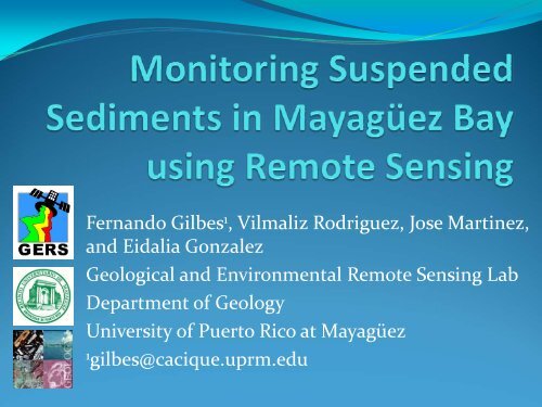
<strong>Fern<strong>and</strong>o</strong> Gilbes 1 , <strong>Vilmaliz</strong> <strong>Rodriguez</strong>, <strong>Jose</strong> <strong>Martinez</strong>,<br />
<strong>and</strong> <strong>Eidalia</strong> Gonzalez<br />
Geological <strong>and</strong> Environmental Remote Sensing Lab<br />
Department of Geology<br />
University of Puerto Rico at Mayagüez<br />
1<br />
gilbes@cacique.uprm.edu
MAYAGUEZ BAY<br />
Deep <strong>and</strong> Clear<br />
Waters<br />
Añasco River<br />
Sewage Outfall<br />
Yaguez River<br />
CLIMATOLOGY OF<br />
AÑASCO RIVER DISCHARGE<br />
(20 years)<br />
Shallow <strong>and</strong> Clear<br />
Waters with<br />
Coral Reefs<br />
Guanajibo River<br />
DRY SEASON<br />
RAINY SEASON
TWO SEASONS IS EQUAL TO<br />
TWO OPTICAL CONDITIONS
MULTI‐SPECTRAL AIRBORNE SENSORS<br />
AOCI<br />
30 m <strong>and</strong> 10 b<strong>and</strong>s<br />
ATLAS<br />
10 m <strong>and</strong> 15 b<strong>and</strong>s
MULTI‐SPECTRAL SATELLITE SENSORS<br />
THEMATIC MAPPER<br />
30 m <strong>and</strong> 7 b<strong>and</strong>s<br />
IKONOS<br />
1 m <strong>and</strong> 4 b<strong>and</strong>s
MOTIVATION FOR OUR WORK<br />
• Can we use remote sensing to measure suspended<br />
sediments in Mayaguez Bay?<br />
• If so, what sensor <strong>and</strong> algorithm are more accurate?<br />
• What are the sources of error in measuring suspended<br />
sediments with remote sensors in Mayaguez Bay?<br />
• Can we develop a continuous monitoring system of<br />
suspended sediments in Mayaguez Bay, <strong>and</strong> therefore<br />
over Puerto Rico?
REMOTE SIGNAL FROM THE OCEAN
SEPARATING THE REMOTE SIGNAL<br />
What we Measure<br />
• Water Optical Properties<br />
• Bottom Reflectance<br />
FromNEMO Overview<br />
Nemo.nrl.navy.gov
REFLECTANCE VS. SEDIMENTS<br />
• Reflectance<br />
• Previous findings<br />
• Increase in SS = Increase in<br />
reflectance<br />
• Red & Near IR wavelengths<br />
show lower slopes in high<br />
SS<br />
• Mayagüez Bay<br />
• Concentration too low to<br />
provide strong response<br />
From Witte et al. (1982)
MAIN OBJECTIVE<br />
To validate the accuracy of several<br />
remote sensors <strong>and</strong> algorithms for<br />
measuring suspended sediments<br />
(SS) in Mayagüez Bay, PuertoRico.
TECHNICAL APPROACH<br />
Field<br />
Work<br />
Testing<br />
MODIS<br />
Testing<br />
AVIRIS<br />
Seasonal<br />
samplings<br />
Testing the<br />
Miller & Mckee<br />
algorithm using<br />
250 m b<strong>and</strong>s<br />
Develop a local<br />
algorithm with<br />
IR b<strong>and</strong>s<br />
Suspended<br />
sediments by<br />
the filter<br />
method<br />
Develop local<br />
algorithm using<br />
250 m b<strong>and</strong>s<br />
Geobio‐optical<br />
Properties
20 SAMPLING DATES<br />
• April 24-26, 2001<br />
• October 2-4, 2001<br />
• February 26-28, 2002<br />
• August 20-22, 2002<br />
• February 25-27, 2003<br />
• October 7-9, 2003<br />
• January 12-14, 2004<br />
• February 12, 2004<br />
• August 19, 2004<br />
• March 10, 2005<br />
• July 19, 2005<br />
• August 17, 2005<br />
• September 20, 2005<br />
• October 19, 2005<br />
• December 6, 2005<br />
• March 8, 2006<br />
• April 21, 2006<br />
• September 26, 2006<br />
• October 26, 2006<br />
• May 1-2, 2007
GRID OF<br />
SAMPLING<br />
STATIONS
Moderate Resolution Imaging<br />
Spectroradiometer (MODIS)<br />
EOS AM<br />
~10:30 AM<br />
LOCAL TIME<br />
EOS PM<br />
~1:30 PM<br />
LOCAL TIME
MODIS SPATIAL RESOLUTION<br />
B<strong>and</strong>s 1-2 = 250 m<br />
B<strong>and</strong>s 3-7 = 500 m<br />
B<strong>and</strong>s 8-36 = 1000 m
MODIS SPECTRAL RESOLUTION<br />
Primary Use B<strong>and</strong> B<strong>and</strong>width<br />
Primary Use B<strong>and</strong> B<strong>and</strong>width<br />
L<strong>and</strong>/Cloud/Aerosols<br />
Boundaries<br />
1 620 - 670<br />
2 841 - 876<br />
SS<br />
Surface/Cloud<br />
Temperature<br />
20 3.660 - 3.840<br />
21 3.929 - 3.989<br />
L<strong>and</strong>/Cloud/Aerosols<br />
Properties<br />
3 459 - 479<br />
4 545 - 565<br />
Chl-a<br />
22 3.929 - 3.989<br />
23 4.020 - 4.080<br />
5 1230 - 1250<br />
6 1628 - 1652<br />
Atmospheric<br />
Temperature<br />
24 4.433 - 4.498<br />
25 4.482 - 4.549<br />
Ocean Color/<br />
Phytoplankton/<br />
Biogeochemistry<br />
7 2105 - 2155<br />
8 405 - 420<br />
9 438 - 448<br />
10 483 - 493<br />
11 526 - 536<br />
12 546 - 556<br />
13 662 - 672<br />
NASA<br />
Chl-a<br />
Cirrus Clouds 26 1.360 - 1.390<br />
Water Vapor<br />
27 6.535 - 6.895<br />
28 7.175 - 7.475<br />
Cloud Properties 29 8.400 - 8.700<br />
Ozone 30 9.580 - 9.880<br />
Surface/Cloud 31 10.780 - 11.280<br />
Temperature<br />
32 11.770 - 12.270<br />
14 673 - 683<br />
15 743 - 753<br />
Cloud Top<br />
Altitude<br />
33 13.185 - 13.485<br />
34 13.485 - 13.785<br />
16 862 - 877<br />
35 13.785 - 14.085<br />
Atmospheric<br />
Water Vapor<br />
17 890 - 920<br />
18 931 - 941<br />
36 14.085 - 14.385<br />
19 915 - 965
SUSPENDED SEDIMENTS<br />
• Miller <strong>and</strong> McKee (2004)<br />
• Study of northern Gulf of<br />
Mexico‐Mississippi Delta<br />
• Linear relationship: in situ<br />
Suspended Matter vs.<br />
MODIS Terra B<strong>and</strong> 1 (620 –<br />
670 nm)<br />
• Provided evidence of<br />
sediment transport<br />
Calibrated images of Mississippi River delta derived<br />
from MODIS Terra B<strong>and</strong> 1 (Miller & McKee, 2004)
Miller <strong>and</strong> McKee (2004) Algorithm
RESULTS IN MAYAGUEZ BAY
2 ND APPROACH‐A NEW ALGORITHM<br />
• Image preprocessing<br />
with ENVI (Environment<br />
for Visualization of<br />
Images)<br />
• Geo‐referencing: UTM 19<br />
(Datum NAD 83)<br />
• 17 GPS points<br />
corroborated<br />
• Atmospheric correction:<br />
• Dark Subtract<br />
GPS points used in geo-reference validation
FIELD SS AND MODIS‐B1 %REFLECTANCE<br />
30<br />
25<br />
Suspended Sediment Concentration (mg/l)<br />
20<br />
15<br />
10<br />
5<br />
y = 105.19x + 2.6373<br />
R 2 = 0.1443<br />
0<br />
0 0.02 0.04 0.06 0.08 0.1 0.12 0.14<br />
MODIS Terra B<strong>and</strong> 1 Reflectance (%)<br />
All Stations: (2001 – 2006)
FIELD SS AND MODIS‐B1 %REFLECTANCE<br />
30<br />
30<br />
25<br />
25<br />
Suspended Sediment Concentration (mg/l)<br />
20<br />
15<br />
10<br />
5<br />
y = 80.703x + 3.614<br />
R 2 = 0.0695<br />
Suspended Sediment Concentration (mg/l)<br />
20<br />
15<br />
10<br />
5<br />
y = 136.58x + 0.8668<br />
R2 = 0.2788<br />
0<br />
0 0.01 0.02 0.03 0.04 0.05 0.06 0.07 0.08 0.09<br />
MODIS B<strong>and</strong> 1 Reflectance (%)<br />
0<br />
0 0.02 0.04 0.06 0.08 0.1 0.12 0.14<br />
MODIS Terra B<strong>and</strong> 1 Reflectance (%)<br />
Dry Season (2001 – 2006) Rainy Season (2001 – 2006)
FIELD SS AND MODIS‐B1 %REFLECTANCE<br />
30<br />
16<br />
14<br />
25<br />
Suspended Sediment Concentration (mg/l)<br />
20<br />
15<br />
10<br />
5<br />
y = 63.781x + 5.962<br />
R 2 = 0.0473<br />
Suspended Sediment Concentration (mg/l)<br />
12<br />
10<br />
8<br />
6<br />
4<br />
2<br />
y = 55.796x + 3.2736<br />
R 2 = 0.0468<br />
0<br />
0<br />
0 0.02 0.04 0.06 0.08 0.1 0.12 0.14 0 0.01 0.02 0.03 0.04 0.05 0.06 0.07 0.08<br />
MODIS Terra B<strong>and</strong> 1 Reflectance (%)<br />
MODIS Terra B<strong>and</strong> 1 Reflectance (%)<br />
In-shore Stations (2001 – 2006) Off-shore Stations (2001 – 2006)
A NOVEL APPROACH<br />
SS = 337.26 *(B<strong>and</strong> 1) + 854.12 *(B<strong>and</strong> 2)<br />
40.00<br />
35.00<br />
30.00<br />
25.00<br />
20.00<br />
15.00<br />
10.00<br />
5.00<br />
0.00<br />
Suspended Sediments conc (mg/l)<br />
A1<br />
A2<br />
G2<br />
A1<br />
A2<br />
AAA1<br />
Y1<br />
G1<br />
G2<br />
A1<br />
A2<br />
AAA1<br />
G2<br />
A1<br />
A2<br />
AAA1<br />
Y1<br />
A1<br />
A2<br />
Y1<br />
G1<br />
G2<br />
A1<br />
A2<br />
AAA1<br />
Y1<br />
G2<br />
A1<br />
A2<br />
AAA1<br />
G2<br />
A1<br />
A2<br />
AAA1<br />
Y1<br />
G1<br />
July 17<br />
05<br />
August 17 05 September<br />
20 05<br />
October 19<br />
05<br />
December 6 05 April 21 06 September<br />
26 06<br />
TSS (Observed)<br />
TSS (Estimated)<br />
October 26 06<br />
30.00<br />
25.00<br />
20.00<br />
15.00<br />
10.00<br />
5.00<br />
0.00<br />
Observed<br />
Estimated<br />
A1<br />
A2<br />
AAA<br />
Y1<br />
G1<br />
G2<br />
S05<br />
S09<br />
S11<br />
S13<br />
S15<br />
S17<br />
S19<br />
S21<br />
S23<br />
S01<br />
S02<br />
S03<br />
S13<br />
S14<br />
S15<br />
S21<br />
S22<br />
S23<br />
S01<br />
S04<br />
S05<br />
S07<br />
S17<br />
S19<br />
S21<br />
S23<br />
Suspended Sediments conc (mg/l)<br />
y = 0.4033 * b<strong>and</strong> 1 – 0.0006<br />
SS (mg/l) = 452.41 * y + 2.9603<br />
Mar-06 Jan-13-04 Jan-14-04 Feb-12-04 Oct-07-03 Feb-27-03
SS WITH NEW ALGORITHM<br />
October 7, 2003 January 14, 2004
AVIRIS<br />
AIRBORNE VISIBLE/INFRARED<br />
IMAGING SPECTROMETER<br />
‣ 224 Spectral B<strong>and</strong>s<br />
‣ Range from 400 to 2500 nm<br />
‣ Strip lines of 11 km wide<br />
‣ Spatial resolution from 4 m to 20 m<br />
(Puerto Rico mission was ~17 m)
AVIRIS MISSION OVER PUERTO RICO<br />
AUGUST 19, 2004
AVIRIS IMAGES USED IN THIS STUDY<br />
TO ESTIMATE SUSPENDED SEDIMENTS
Suspended Sediments measured<br />
during AVIRIS overflight<br />
18<br />
16.7<br />
Suspended Sediments (mg/l)<br />
16<br />
14<br />
12<br />
10<br />
8<br />
6<br />
15.5<br />
7.2<br />
?<br />
5.1<br />
5.5<br />
4<br />
2<br />
1.4<br />
2.4<br />
3.0<br />
1.7<br />
1.1<br />
0<br />
S01 S02 S04 S05 S07 S13 S15 S21 S23 S24<br />
Stations
Anasco River discharge during August 2004
IMAGE PROCESSING<br />
Raw Image<br />
from NASA<br />
Atmospheric<br />
Correction<br />
using ACORN<br />
ENVI<br />
Extraction of<br />
Reflectance<br />
from stations<br />
20 λ’s<br />
Application of<br />
site-specific<br />
algorithm to<br />
the image<br />
Development of<br />
the algorithm<br />
Correlation of image<br />
data with field data<br />
Masking<br />
of<br />
bad pixels<br />
Mosaicking<br />
Final Image<br />
of<br />
Sediments
Relative Reflectance as measured<br />
with AVIRIS<br />
2000<br />
1500<br />
Añasco<br />
1000<br />
Guanajibo<br />
500<br />
Yaguez<br />
0<br />
404.0<br />
432.0<br />
463.0<br />
493.0<br />
524.0<br />
554.0<br />
585.0<br />
616.0<br />
646.0<br />
677.0<br />
707.0<br />
738.0<br />
769.0<br />
797.0<br />
828.0<br />
858.0<br />
889.0<br />
919.0<br />
950.0<br />
981.0
Testing different b<strong>and</strong>s
Suggested Algorithm to estimate suspended<br />
sediments in Mayaguez Bay using AVIRIS<br />
Concentration of Suspended Sediments (mg/l) = a (x) + b<br />
Where, a = 0.0829<br />
x = AVIRIS Reflectance at 777 nm<br />
b = 0.0325
SUSPENDED SEDIMENTS AS DETERMINED WITH AVIRIS
CONCLUSIONS<br />
• Image processing <strong>and</strong> analyses clearly demonstrated that<br />
MODIS is not the most appropriate ocean color sensor for<br />
Mayagüez Bay.<br />
• Another sensor with better temporal, spatial, <strong>and</strong> spectral<br />
resolutions is still needed for the estimation of SS in<br />
tropical coastal waters.<br />
• However, MODIS B<strong>and</strong> 1 gives good qualitative results of SS<br />
when a site‐specific algorithm is applied in Mayagüez Bay.<br />
• Future work with MODIS in this region must include (but<br />
not limited):<br />
• Improve the atmospheric correction<br />
• Consider other sources of error like bottom <strong>and</strong> l<strong>and</strong> signal<br />
• Mineral composition <strong>and</strong> grain characteristics of SS
CONCLUSIONS<br />
• AVIRIS proved to be a good sensor for the estimation of<br />
suspended sediments in Mayaguez Bay.<br />
• The applied techniques produced an algorithm that uses<br />
the 777 nm b<strong>and</strong> with a R 2 of 0.82.<br />
• Some fine tuning is necessary along the image processing<br />
in order to improve the estimations. We are waiting for reprocessed<br />
images (by NASA) in order to repeat the work.<br />
• In order to monitor SS in Mayaguez Bay using remote<br />
sensing we still need to underst<strong>and</strong> their relationship with<br />
the reflectance signal.