Elemento Finito con el paquete IMS

Elemento Finito con el paquete
IMS
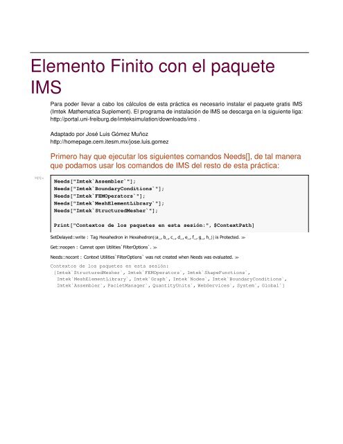
Para poder llevar a cabo los cálculos de esta práctica es necesario instalar el paquete gratis IMS
(Imtek Mathematica Suplement). El programa de instalación de IMS se descarga en la siguiente liga:
http://portal.uni-freiburg.de/imteksimulation/downloads/ims .
Adaptado por José Luis Gómez Muñoz
http://homepage.cem.itesm.mx/jose.luis.gomez
Primero hay que ejecutar los siguientes comandos Needs[], de tal manera
que podamos usar los comandos de IMS del resto de esta práctica:
In[1]:=
Needs@"Imtek`Assembler`"D;
Needs@"Imtek`BoundaryConditions`"D;
Needs@"Imtek`FEMOperators`"D;
Needs@"Imtek`MeshElementLibrary`"D;
Needs@"Imtek`StructuredMesher`"D;
Print@"Contextos de los paquetes en esta sesión:", $ContextPathD
SetDelayed::write : Tag Hexahedron in Hexahedron@8a_, b_, c_, d_, e_, f_, g_, h_

2 FEM0500ims.nb
Se va a calcular una solución aproximada a una ecuación diferencial
ordinaria, lineal e inhomogénea, - d IpHxL d yHxLM + qHxL yHxL = f HxL, con las
dx dx
condiciones de frontera yHaL = y a , yHbL = y b , como se muestra a continuación
:
In[7]:=
Clear@x, y, p, q, f, a, bD;
p@x_D := x 2 ;
q@x_D := 30;
f@x_D := −14x;
a = 0.0;
b = 1.0;
y a = 0.0;
y b = 0.5;
Print@"−∂ x Hp@xD ∂ x y@xDL+q@xD∗y@xDf@xD → ",
−∂ x Hp@xD ∂ x y@xDL +q@xD ∗y@xD f@xDD;
Print@y@aD y a D;
Print@y@bD y b D;
−∂ x Hp@xD ∂ x y@xDL+q@xD∗y@xDf@xD → 30y@xD −2xy ′ @xD −x 2 y ′′ @xD −14x
y@0.D 0.
y@1.D 0.5

FEM0500ims.nb 3
Se usa el comando imsGenerateLinearStructuredMesh[] para generar el
mallado del dominio. El mallado consiste de nodos (puntos en el dominio) y
elementos (en este caso unidimensional, los elementos son intervalos entre
nodo y nodo):
In[18]:=
numElem = 6;
mapeo@x_D := NBa + Hb −aL
Log@3x +4D
Log@numElem +1D F;
malla =
imsGenerateLinearStructuredMesh@numElem, imsCoordinateMapping → mapeoD;
Graphics@
8Orange, imsDrawElements@mallaD,
Purple, imsDrawElementIdText@mallaD,
Red, imsDrawNodeText@mallaD

4 FEM0500ims.nb
Estos son los elementos del mallado:
In[26]:=
elementos = imsGetElements@mallaD;
Print@"Los elementos son: ", elementosD
Los elementos son: 8imsLineLinear1DOF@1, 81, 2

FEM0500ims.nb 5
Hay un vector local de fuerzas, o cargas, por cada elemento. Después ese
vector local será “ensamblado” en el vector global en los renglones que
corresponden a los nodos del elemento:
In[30]:=
cargas = TableBimsMakeElementMatrixBK 0 0 O,
nodosPorElemento@@jDD, nodosPorElemento@@jDDF, 8j, 1, numElem

6 FEM0500ims.nb
Aquí se calcula el efecto de la “función de difusión” (coeficiente pHxL en la
ecuación diferencial ) en las matrices y cargas (en las ecuaciones) de cada
elemento:
In[33]:=
Out[33]=
matricesycargas =
Table@
imsNFEMDiffusion@ 8matrices@@jDD, cargas@@jDD

FEM0500ims.nb 7
El coeficiente qHxL en la ecuación diferencial es la “función de reacción”,
- d IpHxL d yHxLM + qHxL yHxL = f HxL
dx dx
In[36]:=
funcionReaccion@marker_, x_D := q@xD;
Print@"funcionReaccion@marker,xD=", funcionReaccion@marker, xDD
funcionReaccion@marker,xD=30
Aquí se calcula el efecto de la “función de reacción” (coeficiente qHxL en la
ecuación diferencial ) en las matrices y cargas (en las ecuaciones) de cada
elemento:
In[38]:=
Out[38]=
matricesycargas =
Table@
imsNFEMReaction@ 8matrices@@jDD, cargas@@jDD

8 FEM0500ims.nb
Actualizamos la lista de cargas
In[40]:=
Out[40]=
cargas = matricesycargas@@All, 2DD
8imsElementMatrix@880

FEM0500ims.nb 9
Actualizamos la lista de matrices
In[44]:=
Out[44]=
matrices = matricesycargas@@All, 1DD
8imsElementMatrix@883.68081, 1.6623

10 FEM0500ims.nb
A continuación se “ensamblan” las matrices de cada elemento para formar
la matriz global, y los vectores de carga de cada elemento para formar el
vector de carga global:
In[46]:=
matrizGlobal = SparseArray@8

FEM0500ims.nb 11
El siguiente paso es insertar las condiciones de frontera, lo cual modifica a
la matriz global y al vector global de cargas. En este ejemplo
unidimensional, los únicos nodos de frontera son el primero y el último:
In[52]:=
imsDirichlet@8matrizGlobal, vectorCargas

12 FEM0500ims.nb
Estos son los nuevos nodos interiores. Incluyen el valor de la solución:
In[58]:=
Out[58]=
nodosNuevosInterior = nodosNuevos@@imsGetIds@imsGetInteriorNodes@mallaD D DD
8imsNode@2, 80.356207

FEM0500ims.nb 13
A continuación se muestra la gráfica de la solución analítica exacta,
obtenida con el comando DSolve:
In[61]:=
solexacta =
DSolve@8−∂ x Hp@xD ∂ x y@xDL +q@xD ∗y@xD f@xD, y@aD y a , y@bD y b

14 FEM0500ims.nb
http://portal.uni-freiburg.de/imteksimulation/downloads/ims .
Capítulo 6, Sección 6.3 “Finite Element Method” de la Tesis de Doctorado de Oliver Rüebenkönig “Free
Surface Flow and the IMTEK Mathematica Supplement”, Institut für Mikrosystemtechnik (IMTEK),
Albert-Ludwigs-Univesität, Freiburg, Alemania.
ftp://elmo.imtek.uni-freiburg.de/pub/people/ruebenko/writing/dissertation1.1.pdf .
Daryl L. Logan, “A First Course in the Finite Element Method”, Fifth Edition, 2012, Cengage Leraning
Adaptado por José Luis Gómez Muñoz
http://homepage.cem.itesm.mx/jose.luis.gomez