Vol. 2 Núm. 8 - Instituto Nacional de Investigaciones Forestales ...

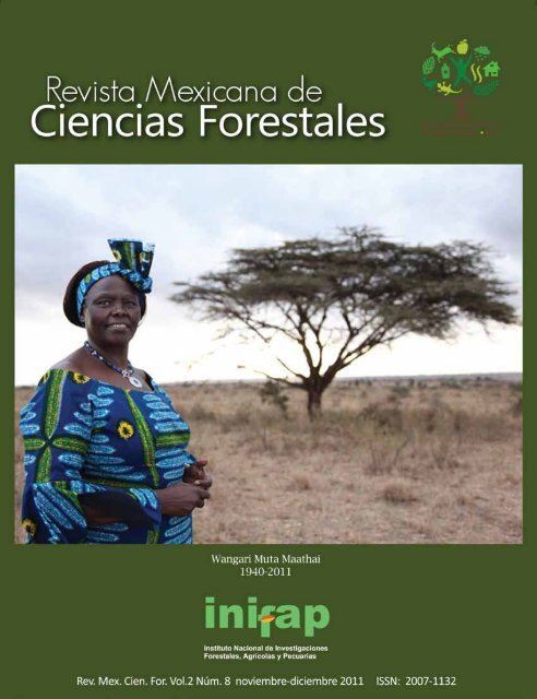
Editorial“Wangari Muta Maathai. Remembranza por su contribución aldesarrollo sostenible, la democracia y la paz”.«Un árbol tiene raíces en el suelo y ramas que rozan el cielo, recordándonos quepara prosperar debemos saber nuestro origen. Al igual que los árboles, por muchoque lleguemos lejos, son nuestras raíces las que nos alimentan»Wangari Muta MaathaiWangari Muta Maathai, ganadora del premio Nobel de la Paz 2004, falleció el domingo 25 de septiembre de 2011, justo cuando enla capital de México se clausuraba la más importante exposición forestal. Ese día lejos de guardarse un minuto de silencio, prevalecióun profundo silencio sobre tan lamentable deceso. Hecho que en general fue compartido en el mundo -si quien hubieramuerto hubiese sido un futbolista millonario o una popular cantante aficionada a las drogas, los medios se hubieran volcadoen la noticia-. Sin embargo, su influencia se ha sentido en todo el orbe, la Revista Time la declaró Héroe del Planeta, al sumar convalentía a su causa a miles de africanos y millones de voluntades. Impulsó la participación colectiva, preponderantemente femenina,en torno a los proyectos de reforestación como un instrumento para mejorar la calidad de vida de las comunidades rurales. Dedicósu vida a defender el bosque, a otras mujeres y a la democracia. Pero sobre todo, ayudó a construir el concepto sostenible,formulado por otra mujer: Norman Brundtland. De hecho su activismo político estuvo ligado a su labor de conservación. En diversosforos preparatorios a la reunión de Johannesburgo, que marcaba los diez años de su similar de Río de Janeiro, seexpresaba la inquietud de no “africanizar” la cumbre. Qué lejos se estaba de imaginar que la solución a la crisis ambiental estaba en elcontinente de donde precisamente surgió el género humano.Michelle Bachelet, Directora Ejecutiva de ONU Mujeres, en homenaje a Wangari Muta Maathai declaró ese domingo25 septiembre: “Nos unimos a muchos en África y en todo el mundo para llorar su fallecimiento y para celebrar su vida como líderexcepcional, primera mujer africana en recibir el Premio Nobel de la Paz. La Profesora Maathai se declaró, con valentía y siendovíctima de acosos y ataques, a favor de la protección del medio ambiente y del progreso de los derechos de las mujeres, de lalucha contra la desertificación, la escasez de agua y el hambre en el medio rural.” Bachelet exaltó sobre todo su figura de líderextraordinaria que a través del impulso de la reforestación empoderó a miles de mujeres y alentó con pasión una nueva manera depensar y actuar, que combina la democracia y el desarrollo sostenible. Líder intrépida, fue donde nadie había osado ir y desafió aautoridades a quienes pocos osaban desafiar. Rehusando ser intimidada, se mantuvo firme sobre la plena participación de las mujeresen la vida cívica y pública: hoy nos deja un legado que permanecerá para siempre con nosotros. Sus ideas innovadoras sobre lacreación de empleo, gracias al restablecimiento medioambiental, forman parte de la agenda mundial de desarrollo en materia detrabajos y de una economía verdes, en el contexto del desarrollo sostenible y de la erradicación de la pobreza. ParaBachelet, la Dra. Maathai inspirará, especialmente, la preparación para la Conferencia de la ONU sobre Desarrollo Sostenibleque se celebrará en Rio de Janeiro en junio de 2012.Madame Wangari fue una pionera desde su época universitaria, cuando obtuvo la licenciatura en Biología en Atchison, Kansas,EE.UU. y al ampliar sus estudios en Pittsburgh, Alemania y en la Universidad de Nairobi, siendo en 1971, la primera mujer deÁfrica Central y Oriental en obtener un doctorado. Nació en Nyeri, Kenia, madre de tres hijos, diputada y ministra adjunta para Medioambiente, Recursos Naturales y Vida Silvestre. También en el ámbito privado, rompió con una sociedad que relega a la mujer. Sumarido, un antiguo parlamentario, se divorció de ella en 1980 con el argumento de que “era demasiada educada, con amplio caráctery éxito para poder controlarla”. Su mayor contribución fue el Movimiento Cinturón Verde de Kenia, un proyecto que impulsó3

en 1977 y que combina la promoción de la biodiversidadcon la del empleo a mujeres. Productos de esta iniciativa son30 millones de árboles plantados en su país y la ocupaciónde 50 mil mujeres pobres en diferentes viveros. Desde 1986,dicho movimiento originó una gran red panafricana que hallevado proyectos similares a países como Tanzaniay Etiopía. “Si uno desea salvar el entorno, primero hay queproteger al pueblo. Si somos incapaces de preservar la especiehumana, ¿qué objeto tiene salvaguardar las especiesvegetales?”, declaró al resumir su filosofía, que expusomás de una vez en la tribuna de la sede de la Organizaciónde las Naciones Unidas (ONU).En su época como directora del Departamento de AnatomíaVeterinaria en Nairobi (1976-1977), empezó su actividaden el Consejo Nacional de Mujeres de Kenia, organizaciónque presidió entre 1981 y 1987. Promotora de cancelarla deuda externa del Tercer Mundo, destacó como decididaopositora al régimen dictatorial de Daniel Arap Moi, porlo cual, durante la década de 1990, se le detuvo y encarceló.En 1997 fue candidata a la presidencia de Kenia, pero supartido retiró su candidatura días antes de las elecciones. Unaño después, lideró la oposición a un proyecto gubernamentalde construcción en la selva lo que desencadenó una revueltapopular que fue duramente reprimida por el gobierno, actoque recibió el repudio nacional e internacional, en respuestaa su convocatoria. Su compromiso se recompensó conuna profusión de premios, como el de Mujeres del Mundode Women Aid (1989), el de la Fundación EcologistaGoldman (1991) –el llamado Nobel de los ecologistas–,el Premio África de Naciones Unidas (1991) o el Petra Kelly(2004). Para el Comité Nobel, la paz en la tierra dependede la capacidad para asegurar el ambiente, y Maathaise sitúa al frente de la lucha en la promoción del desarrolloeconómico, cultural y ecológicamente viable de África,con una visión planetaria de lo sostenible que abraza lademocracia, los derechos humanos y, en particular, los dela mujer.Pensaba de forma global y actuaba en el ámbito local, elmovimiento Cinturón Verde, es un programa que combinaexistencia comunitaria y protección ambiental, al propagar entrecampesinos la idea básica de que plantar árboles mejora susvidas y la de sus hijos. Su quehacer en el mundo subdesarrolladocombinó ciencia, compromiso social y política activa. Protegerbosques a través de la educación, la planificación familiar,la nutrición y la lucha contra la corrupción. Su propuestatambién compete el otorgamiento de la responsabilidad de unproceso de autogestión de las mujeres, que ni derecho a lapropiedad tenían en Kenia. Su lucha contribuyó a generar unasensibilización de la población sobre su derecho a oponerseal abuso del poder. La campaña contra la apropiaciónilegal de terrenos públicos y bosques, para su urbanización, legranjeó la enemistad del presidente Daniel Arap Moi, quien lacalificó de “perturbada y amenaza a la seguridad del país”.Y en otra vertiente, Wangari Muta Maathai es una expresiónde la poesía africana, una oportunidad para apurar en laespiritualidad y la sabiduría de un continente que es, en símismo, erupción milenaria -selva, desierto, ríos- almas que danzany veneran a sus antepasados. Pero también, muy lamentablemente,una tierra ultrajada por la violencia y el racismo. Empero, apesar del intenso dolor y de las heridas continuas subsiste elcanto de sus poetas –y Wangari lo es–, que preservanla belleza, la religiosidad y el nativo que nos vuelve aenseñar a la nueva humanidad. En su misión llevó siempre elmejorar la situación de las mujeres rurales pobres. Creyó enla inmensa fuerza femenina y trabajó duro para movilizar a lasmujeres pobres. Esta creencia idealizada, la experta enciencias ambientales Lalitha la identifica en el poema“Las mujeres se siembran” de Halldis Moren:La mujer es la plantación de un árbol en el mundo.De rodillas, como si alguien en la oración,entre los restos de los muchos árbolesque la tormenta se ha roto.Ella debe intentarlo de nuevo, tal vez uno al finse dejará de crecer en paz.Ella ve las manos extendidas sobre la tierracomo si estuviera tratando de imponer la calmaPor su temor. Oh muerte! La Tierra, estar quieto,Estad quietos, así que mi árbol puede crecer.En su conferencia nobel esta mujer africana, primera enrecibir el Premio, declara que espera animar a mujeres y niñasa levantar la voz y tener más espacio para el liderazgo.Reconoce el trabajo de innumerables personas y grupos entodo el mundo. Quienes trabajan en silencio y, a menudo, sin elmenor reconocimiento, protegiendo el ambiente,promoviendo la democracia, defendiendo los derechoshumanos y garantizando la igualdad, sembrando semillas4

de paz, a todos ellos les obsequia el premio, no solo paraque se sientan representados, sino para que lo utilicen en promoversu misión y cumplir con las expectativas de este mundo,que será suyo. También agradece a sus conciudadanos“…que permanecieron tercamente con la esperanza de quela democracia pudiera hacerse realidad y su entorno gestionadode forma sostenible…” reconociéndose producto de esta lucha.Resalta Wangari en el Comité Nobel un reconocimiento deque la paz pasa obligadamente por el desarrollo sostenible yeste se finca en la democracia, es una idea cuyo momentoha llegado.Recuerda como fue testigo, desde su infancia, de ladevastación de los bosques y la privatización de las tierras,que acaban con la biodiversidad local y sus funcionesecológicas. En 1977, cuando comenzó el Movimiento delCinturón Verde, en parte fue una respuesta a las necesidadesde las mujeres rurales, la falta de leña, agua potable, unaalimentación equilibrada, vivienda y de ingresos. A lo largode África, las mujeres son las cuidadoras primarias, conresponsabilidad significativa para el cultivo de la tierra yalimentar a sus familias. Son las primeras en tomar concienciadel daño ambiental, que vuelve a los recursos escasos yoriginan que no puedan sostener a sus familias. Las respuestascapitalistas, como la introducción de la agricultura comercialy el comercio internacional controlado por el precio de lasexportaciones, no garantizan de forma razonable y justa elingreso de los agricultores a pequeña escala. Narra cómo llegóa entender que cuando el ambiente es destruido o saqueadose socava el futuro de las generaciones venideras.Así, la plantación de árboles se convirtió en una opciónnatural para hacer frente a necesidades básicas inicialesidentificadas por las mujeres. Además, la reforestaciónes simple, asequible y garantiza resultados rápidos y exitososdentro de un plazo razonable. Esto mantiene el interés y elcompromiso. Así que, las mujeres plantaron más de 30 millonesde árboles que proveen de combustible, alimentos, vivienday los ingresos para apoyar la educación de sus hijos y lasnecesidades del hogar. La actividad también generóempleos y mejoró los suelos y las cuencas hidrográficas. Através de su participación, las mujeres adquieren podersobre sus vidas y la de sus familias, especialmente de suposición social y económica.Prosigue en su conferencia, el trabajo era difícil porquehistóricamente el pueblo había sido persuadido de que porsu condición de pobre, no solo carecía de capital, sino delconocimiento y las habilidades para hacer frente asus desafíos; y en cambio, estaba condicionado a creer quelas soluciones a sus problemas debían venir de “afuera”.Sin embargo, las mujeres se percataban de que la soluciónde sus requerimientos depende de que su entorno esté sano ybien gestionado; siendo conscientes –en carne propia- de queun ambiente degradado conduce a una lucha por los recursosescasos, que culmina en la guerra. Incluso intuían las injusticias delos acuerdos económicos internacionales. Con el fin de ayudara las comunidades para entender estas relaciones, la galardonadaexplica como se desarrolló un programa de educaciónciudadana, en el cual las personas identifican sus problemas,las causas y posibles soluciones. Progresivamente, establecenconexiones entre sus propias acciones y los problemas del mediosocial. Se enteran como afrontar problemas: la corrupción, laviolencia contra las mujeres y los niños, la interrupción yruptura de las familias; así como, la desintegración de lasculturas y comunidades. También identifican el abusode drogas y sustancias enervantes, especialmente entre losjóvenes, así como enfermedades devastadoras y que ocurren enproporciones epidémicas, de particular preocupación son el SIDA,el paludismo y la desnutrición. Así mismo, llama la atención sobrela grave afectación humana por la destrucción generalizadade los ecosistemas, empero de manera preponderantepor la inestabilidad climática y la contaminación en los suelosy las aguas que acentúan una atroz pobreza. En el proceso,se descubren parte de las soluciones, descubren su potencialoculto encontrando amplias facultades para superar la inerciay entrar en acción. Llegan a reconocer que los habitantesrurales son los principales guardianes y beneficiarios del medioambiente que los sostienen. Comunidades enteras tambiénllegan a entender que, si bien, es necesario responsabilizar asus gobiernos, es igualmente importante, que en sus relacionescon los demás, ejemplifiquen los valores de liderazgo quedesean ver en sus propios dirigentes, es decir, la justicia, laintegridad y la confianza. Aunque inicialmente las actividadesdel Movimiento del Cinturón Verde no se refirieron alos problemas de la democracia y la paz, pronto quedó claroque el manejo responsable del ambiente era imposible sin unamplio espacio democrático. Por lo tanto, el árbol se convirtióen un símbolo de la lucha democrática en Kenia.5

esperanza y nuestro futuro. El enfoque holístico del desarrollo,como lo demuestra el Movimiento Cinturón Verde, podría seradoptado y replicado en varias partes de África, y más allá.”Y volvió a su niñez cuando bebía agua de los ríos, jugabaentre las hojas de “arrurruz” y trataba de atraparrenacuajos. Ahora ese mundo de sus padres ya no es el de susnietos. Las corrientes se han secado, las mujeres caminanlargas distancias para conseguir agua, no siempre limpia, y losniños nunca sabrán lo que han perdido. “El desafío consiste enrestaurar la casa de los renacuajos y devolver a nuestros hijosun mundo bello y maravilloso”.En una entrevista esta noble científica social declaró: “Es acausa de la conducta inmoral, que hay contaminación en todaspartes; el aire, el agua, la tierra y los alimentos, se han vistogravemente corrompidos debido a una conducta impropia.La contaminación se podría haber evitado. La fuertecaída de las virtudes como el amor, la compasión y latolerancia es directamente responsable de la degradaciónque uno ve hoy en día. De hecho, incluso se podría decir queestos elementos tienen miedo del hombre. La impurezase refleja en la contaminación exterior. La buena conducta debe serla base real para la vida. Sin embargo, el hombre modernocarece totalmente de carácter y virtudes. No es de extrañar lapaz y la felicidad se le escapan.”que los problemas primero se resolvían con la fuerza mental,también creía en la asociación humana y que la felicidad seencontraba en la unión. Una vez le preguntaban a un científicoque la conoció ¿cuál creía que era el secreto de esa fuentede inspiración interminable? Y él respondió: La profesoraMaathai retrata el amor en cada acción suya. El amor erael aliento mismo del nudo de unión natural con la progenieverde. Cada lucha que acometió pone de relieve el amor puroe incondicional y sin mancha que formó la base de sus obrasaltruistas. Su vida y su obra representan la frase “El amor es eldesinterés y el yo es falta de amor ‘.Cuando recibió la llamada, con la que le comunicaron quehabía recibido el premio nobel, Wangari detuvo el automóvilen un hotel que encontró de camino a uno de tantos pueblosque apoyaba con sus proyectos de conservación forestal ypidió permiso para plantar un árbol que celebrara elacontecimiento. Ese árbol fue un Tulipán Africano.Carlos Mallén RiveraEditor en JefeLa Dra.Wangari Maathai promovió iniciativas queincluyeron la protección de los ecosistemas tropicales de lacuenca del Congo, siendo embajadora itinerante deesta región de acceso global para la diversidad biológicay penosamente amenazados por la tala ilegal, la exploraciónminera, la caza furtiva y el comercio de animales silvestres.En la construcción de su cruzada para proteger losbosques, la profesora Maathai se enteró de un plan delgobierno para privatizar grandes áreas de tierra en el bosqueKarura. Ella protestó en contra de un plan de industrializacióndel Congo, como lo hizo por muchos otros proyectos de estetalante, incluso con el visto bueno de gobiernos y sociedad,decía: “No podemos desarrollar nuestros países, si vamosa seguir la corrupción en ambos lados”. Ella tenía notabletolerancia, paciencia y perseverancia, tomó enormesriesgos personales para luchar por la justicia, así como porlos derechos humanos y del medio ambiente. Ella consideróCarlos Galindo (2010) Flor de Tulipan africano.Spathodea campanulata Deauv“The living conditions of the poor must be improved if wereally want to save our environment”Wangari Maathai, Premio Nobel de la Paz 2004.7

Wangari Muta Maathai. Dominio público.8

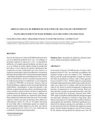
RESUMENMODELOS PARA ESTIMACIÓN Y DISTRIBUCIÓN DE BIOMASA DEAbies religiosa (Kunth) Schltdl. et Cham. EN PROCESO DE DECLINACIÓNBIOMASS ESTIMATION AND DISTRIBUTION MODELS OFAbies religiosa (Kunth) Schltdl. et Cham. IN DECLINEPatricia Flores-Nieves 1 , Miguel Ángel López-López 1 , Gregorio Ángeles–Pérez 1 ,María de Lourdes de la Isla-Serrano 2 y Germán Calva-Vásquez 3Actualmente, el gobierno federal promueve el pago por captura de carbono en los bosques para mitigar el calentamiento global.Por ello, existe la necesidad de estimar la biomasa y tasas de captura de carbono en los bosques de Abies religiosa. En este estudiose generaron modelos para calcular la biomasa de fuste, de madera de ramas y de acículas de árboles completos y de ramas deoyamel en rodales del Cerro Tláloc, Texcoco, Estado de México. Para el caso de árboles completos, la biomasa estuvo en función deldiámetro normal (DN), mientras que para ramas individuales fue una función del diámetro basal (DB). El uso de los modelos generadosa nivel árbol se recomienda para árboles con DN entre 12 y 105 cm, n cambio los modelos a nivel de ramas se recomiendan paradiámetros basales entre 1 y 120 mm. El modelo para fustes fue de tipo potencial y los de madera de ramas y follaje de árbolescompletos de tipo exponencial. Los coeficientes de determinación de los modelos a nivel árbol indican que existe una considerablevariabilidad, principalmente, en las biomasas de ramas, lo que puede ser consecuencia del proceso de declinación en la zonade estudio. La biomasa total de los árboles se distribuye en forma atípica entre los compartimentos aéreos: 97 % en los fustes, 3 % enmadera de ramas y 0.07 % en follaje. Este patrón de distribución de biomasa refleja el efecto del deterioro de los bosquesde A. religiosa.Palabras clave: Fuste, rama, acículas, ecuación alométrica, oyamel, productividad primaria neta.ABSTRACTAt present, the federal government promotes a payment for carbon sequestration by forests to mitigate global change. This is whythere exists a need for estimating biomass and carbon sequestration rates in Abies religiosa forests. In this study stem, branch woodand needle biomass estimation models were generated for whole A. religiosa trees and branches in stands at Cerro Tláloc, Texcoco,Estado de México. For whole trees biomass was a function of breast height diameter (BHD), and for individual branches, biomasswas a function of basal diameter (BD). Use of tree-level models is suitable for trees with BHD within the range of 12 and 105 cm,and branch-level models are recommended for BD within 1 and 120 mm. Stem models were potential while tree-level branchwood and foliage ones were exponential. Determination coefficients for whole-tree models show that there exists a large variability,especially for branch biomass, which is likely to be a result of the decline process taking place in the study area. Total tree biomass isatypically distributed within aboveground tree components: 97 % corresponds to stems, 3 % to branch-wood and 0.07 % to foliage.This biomass distribution pattern may be a reflection of the decline process affecting A. religiosa in the study area.Key words: Stem, branch, needle, allometric equation, Sacred-fir, net primary productivity.Fecha de recepción: 5 de febrero 2010Fecha de aceptación: 25 de julio de 20111Posgrado Forestal, Colegio de Posgraduados. Correo-e: floresnp@colpos.mx2Posgrado de Hidrociencias, Colegio de Posgraduados.3Facultad de Estudios Superiores Zaragoza, UNAM.

Rev. Mex. Cien. For. Vol. 2 Núm. 8INTRODUCCIÓNLa conversión de los bosques maduros en áreas abiertaspara diferentes usos económicos del suelo, como agriculturao ganadería, es un fenómeno que se ha presentado a lolargo de los últimos siglos (Herrera et al., 2001). Los bosquesestán dentro de los ecosistemas naturales con mayorproducción primaria neta. Se calcula que producen de400 a 1,000 g m -2 año -1 de carbono, cantidad dos vecessuperior a la de los pastizales y varias veces mayor que la delos océanos (Waring y Schlesinger, 1985). Una parte de estaproducción se acumula como biomasa y humus, que constituyenla producción primaria neta. La otra parte se destina a procesosde mantenimiento del ecosistema, a través de la respiración(Escandón et al., 1999).Garzuglia y Saket (2003) definen la biomasa aérea comola cantidad total de materia orgánica aérea presente en losárboles, e incluyen hojas, ramas, tronco principal y corteza.Para la estimación de biomasa, el procedimiento más comúnconsiste en el muestreo destructivo de unos cuantos árbolespara después modelar el contenido de biomasa en funciónde variables fáciles de medir, para ello se utilizan métodos deregresión (Díaz et al., 2007).La biomasa se ha convertido en un elemento importante enlos estudios sobre los cambios que ocurren a escala mundial,dado el posible efecto atenuador (sumidero de carbono) quelos bosques pueden tener al secuestrar los excedentes de losgases de efecto invernadero, de un modo temporal (biomasa)y permanente (suelo) y a las consecuencias que se derivan dela modificación de las condiciones climáticas sobre lasalud, estructura y biodiversidad de un sistema forestal(Vidal et al., 2004).Las ecuaciones de biomasa permiten estimar, con bastanteexactitud, el peso de las especies forestales a partir de unnúmero reducido de parámetros de los árboles en pie (Lópezy Keyes, 1987; Castellanos et al., 1996; Rojo et al., 2005). Sinembargo, la disponibilidad de modelos para coníferascomo Abies religiosa (Kunth) Schltdl. et Cham. es reducida. EnMéxico se han desarrollado ecuaciones para Pinus montezumaeLamb. (Garcidueñas, 1987; Manzano et al., 2007; López-Lópezet al., 2009), Pinus cembroides Zucc. (López y Keyes, 1987), Pinuspatula Schltdl. et Cham. (Castellanos et al., 1996), Alnus glabrataFernald, Clethra hartwegii Britt., Rapanea myricoides (Schltdl.)Lundell, Quercus peduncularis Née, Liquidambar macrophyllaOerst e Inga sp. (Acosta et al., 2002), Hevea brasiliensis Müll.Arg. (Rojo et al., 2005) y para Abies religiosa (Avendaño et al., 2009).Los modelos para el cálculo de la biomasa de árbolesestán influenciados por los cambios en la estructura, comoconsecuencia del manejo, presencia de plagas y enfermedades,condiciones climáticas, de suelo o incluso factores genéticos.INTRODUCTIONThe conversion of old forests into open areas for differenteconomic land use such as agriculture or livestock farming hasoccurred during the last centuries (Herrera et al., 2001).Forests are one of the natural ecosystems with highest netprimary production. It has been calculated that they produce from400 to 1,000 g m -2 year -1 C, which is an amount twice higherthan grasslands and several more than that of oceans (Waringand Schlesinger, 1985). One part of production accumulates asbiomass and humus, which constitute the net primary production.The other part is bound to maintenance process of theecosystem, through respiration (Escandón et al., 1999).Garzuglia and Saket (2003) define aerial biomass as thetotal amount of aerial organic matter in trees, including leaves,branches main stem and bark. The most regular procedurefor biomass estimation is destructive sampling of some trees fora later modeling of biomass content in terms of easilymeasurable variables, in which regression methods are used(Díaz et al., 2007).Biomass has become an important element in studiesabout changes that occur world-wide, from the possiblemitigating effect (carbon sink) of forests when they performthe sequestration of the exceeding greenhouse- effect gases,in a temporary (biomass) or permanent (soil) way and to theconsequences of the changing climate conditions upon health,structure and biodiversity of a forest system (Vidal et al., 2004).Biomass equations allow a rather accurate estimationof the weight of forest species from a small number ofstanding-tree parameters (López and Keyes, 1987; Castellanoset al., 1996; Rojo et al., 2005). However, the availability ofmodels for softwoods such as Abies religiosa (Kunth) Schltdl.et Cham. is rather small. Some equations have been developedin Mexico for Pinus montezumae Lamb. (Garcidueñas, 1987; Manzanoet al., 2007; López-López et al., 2009), Pinus cembroides Zucc.(López y Keyes, 1987), Pinus patula Schltdl. et Cham. (Castellanoset al., 1996), Alnus glabrata Fernald, Clethra hartwegii Britt.,Rapanea myricoides (Schltdl.) Lundell, Quercus peduncularisNée, Liquidambar macrophylla Oerst e Inga sp. (Acosta et al.,2002), Hevea brasiliensis Müll. Arg. (Rojo et al., 2005), as wellas for Abies religiosa (Avendaño et al., 2009).Models for tree biomass are influenced by changes instructure, as a consequence of management, plagues anddiseases, climate, soil and even some genetic factors.Forest decline is defined as a multifactor sickness caused bybiotic and abiotic agents that generates a decrease of vigorand survival of trees (Granados et al., 2001 and Vázquez etal., 2004). Ciesla (1989) and Granados et al. (2001) point outthat there are symptoms related to this phenomenon, among10

Flores-Nieves et al., Modelos para estimación y distribución...La declinación forestal se define como una enfermedadmultifactorial causada tanto por agentes abióticos comobióticos, lo que implica la reducción del vigor y supervivenciade los árboles (Granados et al., 2001 y Vázquez et al., 2004).Ciesla (1989) y Granados et al. (2001) y López et al. (2006) señalanque son varios los síntomas relacionados con dicho fenómeno,tales como la reducción del crecimiento, degeneración de lossistemas radicales, clorosis en el follaje, reducción delas reservas fotosintéticas, mortalidad de brotes y ramase incremento de la incidencia de ataques de insectos, que sepresentan de manera secuencial o simultánea. Alvarado et al.(1993) citan que puede alterarse la forma cónica de la copa ygenerarse defoliación severa y muerte de ramas en las partesbajas del árbol. Al momento de modelar las variables delos árboles o ecosistemas sujetos a este proceso de declinación,se espera que todos los síntomas mencionados tengan un efectodirecto en los parámetros de los modelos generados.El objetivo de este estudio fue aportar nuevos modelos parala estimación de biomasa de los componentes aéreosde A. religiosa en bosques afectados por el proceso dedeclinación, como es el caso de algunos bosques cercanos alValle de México. Se pretende que las ecuaciones sirvan comoherramienta para la realización de estudios de productividadprimaria neta, captura de carbono y de distribución debiomasa en bosques que se encuentren en dicha condición.MATERIALES Y MÉTODOSÁrea de estudioEl presente trabajo se llevó a cabo en el Cerro Tláloc, en laregión fisiográfica conocida como Sierra Nevada, que se ubicaal oriente del Estado de México (Figura 1). La elevación delcerro es de 4,120 m y el área de estudio se localiza en lavertiente occidental del mismo, en dónde la especie dominantees A. religiosa.Clima.- A lo largo del declive occidental del Cerro Tláloc sedistinguen tres subtipos climáticos: en las áreas planas máscercanas a los lomeríos el clima es C (w 0) (w) b(i´); templadosubhúmedo con una precipitación media anual de 700 mm, conrégimen de lluvia en verano, temperatura media anual entre12 y 18 °C y con una oscilación térmica de 5 a 7 °C. En la zonade lomeríos, hacia las estribaciones de la Sierra de Río Fríoel clima es C (w 1) (w) b(i´); templado subhúmedo, con unaprecipitación media anual entre 800 y 900 mm, régimen de lluviasen verano, con temperatura media anual entre 12 y 18 °C y conuna oscilación térmica de 5 a 7 °C. En las laderas montañosasel clima es de tipo C(w 2) (w) b(i´); templado subhúmedo, con unaprecipitación media anual entre 900 y 1,200 mm, régimen delluvias en verano, temperatura media anual de 10 y 14 °C, conuna oscilación térmica de 5 a 7 °C. Las fluctuaciones climáticas sedeben a la orografía (Ortíz y Cuanalo, 1977).which are a reduction in growth, degeneration of the rootsystem, foliage chlorosis, diminishment of photosyntheticreserves, shoot and branch mortality and an incrementof insect attack, all of which could act sequentially orsimultaneously. Alvarado et al. (1993) stated that the conic shapeof the crown can change and generate an intensive defoliationand death of the lower branches. At the time of modelingthe tree variables or ecosystems subjected to decline, itis expected that all the aforementioned symptoms have adirect effect on the parameter of the generated models.The aim of this study was to provide new models for biomassestimation of the aerial components of A. religiosa in forests indecline, as some nearby Valle de Mexico are. It is expectedthat these equations might be useful to accomplish net primaryproductivity, carbon sequestration and of biomass distributionstudies in forests that are in this condition.MATERIALS AND METHODSStudy areaThe study here described was carried out in Cerro Tláloc(Tlaloc Hill), in Sierra Nevada that lies at the East of Estado deMéxico (Figure 1). The highest altitude is 4,120 m and the studyarea is located in the western hillside, where A. religiosa is thedominant species.Climate.- Along the western fall of Cerro Tlaloc, three climatesubtypes can be found: in the closest plains to the hills, the type ofweather is C (w 0) (w) b(i´), which is a subhumid temperateclimate with 700 mm of annual mean precipitation,summer rainfall, annual average temperature between12 and 18 °C and a thermic oscilation from 5 to 7 °C. In the hillzone, nearby Río Frio Mountain Range, the weather is C (w 1)(w) b(i´) which is a subhumid temperate climate with 800-900 mmof annual mean precipitation, summer rainfall, annual averagetemperature between 12 and 18 °C and a thermic oscilation from5 to 7 °C. In the hillsides, the weather is of the C(w 2) (w) b(i´) type,which is a subhumid temperate climate with 900 and 1200 mmof annual mean precipitation, summer rainfall, annual averagetemperature between 10 and 18 °C and a thermic oscilationfrom 5 to 7 °C Climatic fluctuations are due to orography (Ortízand Cuanalo, 1977).Soils.- According to Mooser (1975), the edaphic material ofValle de México was the result of the volcanic activityof the Tertiary and Quaternary periods. The formations of themiddle Tertiary (Oligocene and Miocene) are located fromTláloc up to near San Pablo Ixayoc town. Soils are incipient,of coarse texture near the cineritic cone of Tláloc, and in theresting areas, they are black, deep, of medium texture and richin organic matter and with medium texture (migajones o francos).11

Flores-Nieves et al., Modelos para estimación y distribución...Modelos para biomasa de árboles completosPara generar los modelos de biomasa de árboles completosse seleccionaron 10 individuos de diferentes dimensiones, queincluyeron la mayor variabilidad de diámetros presentes enla zona (12 a 105 cm). A los árboles ejemplares, se lesmidió el diámetro normal (DN) con una cinta diamétrica yposteriormente fueron derribados.En seguida se le determinó su altura total con unlongímetro de 50 m, se desramó y el fuste fue seccionadoen trozas de dimensiones comerciales (2.55 m de longitud),con una usando una motosierra marca Truper con espadade 20”. Durante el troceo del fuste se obtuvo una rodaja deaproximadamente cinco centímetros de espesor comomuestra de cada troza. A cada troza se le midieron losdiámetros inferior y superior con una cinta diamétrica marcaForestry Suppliers Metric Fabric Diameter Tape, modelo283D/160 cm, con el objeto de estimar su volumen. Eldiámetro de la base de cada una de las ramas del árbol semidió con un vernier digital marca Mitutoyo.En campo se obtuvo el peso húmedo de cada una de lastrozas (cuando fue posible), mediante una báscula marcaOhaus de 100 kg de capacidad y 50 g de precisión.Cuando estas pesaban más de 100 kg en húmedo, solo sedeterminó su volumen con la fórmula de Smalian:Donde:V = (B + b) / 2*LV = Volumen de la troza (m 3 )B, b = Área de la sección mayor y menor de la troza (m 2 )L = Longitud de la troza (m)Las rodajas del fuste se trasladaron en bolsas depolietileno al laboratorio del Postgrado Forestal del CampusMontecillo del Colegio de Postgraduados, para secarlas a80 °C, hasta alcanzar peso constante en un horno de circulaciónforzada marca Felisa modelo F20. Posteriormente se determinóla relación entre el peso seco y peso húmedo. Esta proporciónse aplicó al peso húmedo total de las trozas previamentepesadas en campo, para determinar su biomasa.Cuando las trozas pesaron más de 100 kg, el cálculo desu biomasa se realizó de manera indirecta, a partir de laestimación de la densidad de la madera. Las rodajas extraídasde cada troza se utilizaron para calcular la densidad de lamadera de la troza correspondiente.En el laboratorio, las rodajas (o muestras de ellas en el casode rodajas muy grandes) se impermeabilizaron con parafinapara obtener su volumen mediante el principio de Arquímedes.Para ello se usaron recipientes con agua de tamaño adecuadopower saw with a 20” blade. During these operations, a 5 cm thickslice from each log was taken as a sample. To each log weremeasured the lower and upper diameters with a diametrictape, in order to estimate its volume. The diameter of the baseof each one of the branches was measured with a Mitutoyodigital vernier.In the field was obtained the fresh weight of each log (when itwas possible), with an Ohaus 100 kg scale and 50 g precision.When their wet weight was over 100 kg, volume was onlydetermined with the Smalian formula:Where:V = (B + b) / 2*LV = Volume of the long (m 3 )B, b = Area of the greatest and smallest section ofthe log (m 2 )L = Length of the log (m)Stem slices were kept into plastic bags and were taken to theForest Graduate Studies Laboratory at Montecillo Campusthat belongs to the Graduate Studies School (Colegio dePostgraduados), where they were dried at 80 °C, until theyreached a constant weight in a forced- circulation kiln marcay modelo. Y por cuánto tiempo Afterwards, the dry weight/wetweight relation was determined. This ratio was applied to thetotal wet weight of the logs previously weighted at the field, inorder to determine biomass.When logs were weighed more than 100 kg, thedetermination of biomass was carried out in an indirect way,from the estimation of wood density. The slices taken fromeach log were used to calculate the wood density of thecorresponding log.In the laboratory, the slices (or samples of them when sliceswere too big) were waterproofed with paraffin in order toget their volume by the Archimedes principle. For that ending,containers with water of a right size for the sample volume, whichwere placed on the 100 kg Ohaus scale of 50 g precision, whenbig samples are involved. When samples were small, a 2 kgOhaus and precision of tenth of gram was used. Once thevolume is had, weight was determined in order to estimate theirdensity by the following formula:Where:δm = m/vδm = Density of wet wood (kg m -3 )m = Mass (kg)v = Volume (m 3 )13

Rev. Mex. Cien. For. Vol. 2 Núm. 8para el volumen de las muestras, se colocaron sobre unabáscula Ohaus de 100 kg de capacidad y 50 g de precisión,en el caso de muestras grandes. En el caso de las muestraspequeñas se utilizó una balanza Ohaus de dos kilogramos decapacidad y un décimo de gramo de precisión. Una vezque se obtuvo el volumen se procedió a determinar su peso,para estimar su densidad mediante la fórmula:Donde:δm = m/vδm = Densidad de la madera en húmedo (kg m -3 )m = Masa (kg)v = Volumen (m 3 )La biomasa de cada muestra o rodaja se determinócolocando las muestras en un horno de secado de circulaciónforzada marca Felisa modelo F20 a 80 °C, para eliminar laparafina. Una vez conocidos la densidad de las rodajas y elvolumen de las trozas correspondientes, se calculó la biomasade las trozas mediante la fórmula:Donde:Bt = δt * vtBt = Biomasa de troza (kg)δt = Densidad (kg m -3 )vt = Volumen de la troza (m 3 )Con los datos de biomasa de fustes se corrió un procedimientode regresión, para generar un modelo de estimación debiomasa de ese compartimento en función del diámetro normal.Donde:Bf = f (DN)Bf = Biomasa de fuste (kg)DN = Diámetro normal (cm)La biomasa de madera de ramas y del follaje se estimó apartir del diámetro basal de la rama, para lo cual se utilizaronmodelos previamente elaborados por el procedimiento que sedescribe a continuación.Modelos para biomasa a nivel de ramasEl modelo para estimar la biomasa de madera de ramasindividuales se elaboró a partir de 35 ramas de diversosdiámetros basales (1 a 120 mm), procedentes de varios árbolesdel área de estudio. A las ramas recolectadas se les determinóThe biomass of every sample or slice was determined byplacing the samples into a marca y modelo dryingforced-circulation kiln at 80 °C in order to remove theparaffin. Once the slice density and the volume of theirlogs were known, the biomass of the logs was calculated by thefollowing formula:Where:Bt = δt * vtBt = Log biomass (kg)δt = Density (kg m -3 )vt = Volume of the log (m 3 )With the stem biomass data a regression was run to generatea biomass estimation model of that compartment in terms ofthe normal diameter:Where:Bf = f (DN)Bf = Stem biomass (kg)DN = Normal diameter (cm)Branch wood and foliage biomass was estimated from thebasal branch diameter; thus, previously made modelswere used by the procedure was described as follows.Models for biomass at a branch levelThe model to estimate wood biomass of individual brancheswas designed from 35 branches of different basaldiameters (1 to 120 mm), taken from several trees of the studyarea. To the collected branches, basal diameter was calculatedwith a Mitutoyo digital vernier caliper, and from them,leaves were pulled apart in the field, and were weighted by aOhaus ES100L scale in wet, wood and foliage separately. Whenbranches surpassed the capacity of the Felisa F20 dryingkiln, slices of wood were taken and several representativesamples, 10 at the most, were weighted in wet. This materialwas taken to the laboratory to be dried at a Felisa F20forced-circulation kiln at 80 y 70 °C, respectively, in orderto determine its moister content by the following equation:Where:CHm = (PHm - PSm) * 100) / PHmCHm =Moisture content of the sample or slice (%)PHm = Wet weight of the sample (g)PSm = Dry weight of the sample (g)14

Flores-Nieves et al., Modelos para estimación y distribución...su diámetro basal con un vernier digital marca Mitutoyo yposteriormente fueron deshojadas en campo y se pesaronen húmedo la madera y el follaje por separado, en unabalanza Ohaus ES100L. De la madera, cuando las ramassuperaron la capacidad del horno de secado marca FelisaF20, se tomaron rodajas, y del follaje se obtuvo un máximo de10 muestras representativas que también fueron pesadas enhúmedo. El material se llevó al laboratorio para su secadoen un horno de circulación forzada marca Felisa F20 a 80y 70 °C, respectivamente, para determinar su contenido dehumedad mediante la ecuación:Donde:CHm = ((PHm - PSm) * 100) / PHmCHm = Contenido de humedad de la muestra orodaja (%)PHm = Peso húmedo de la muestra (g)PSm = Peso seco de la muestra (g)El contenido de humedad se aplicó al total de madera delas ramas y follaje para obtener su peso seco, a partir de supeso húmedo.Donde:Bcr = PHcr – (PHcr * CHcr / 100)Bcr = Biomasa del compartimiento de la rama(madera o follaje, kg)PHcr = Peso húmedo del compartimiento de la rama(madera o follaje, kg)CHcr = Contenido de humedad del compartimientode la rama (madera o follaje, %)Moisture content was applied to the total branch wood andfoliage to get their dry weight from their wet weight.Where:Bcr = PHcr – (PHcr * CHcr / 100)Bcr = Biomass of compartment of the branch (woodor foliage, kg)PHcr = Wet weight of the branch compartment (woodor foliage, kg)CHcr = Moisture content of the branch compartment(wood or foliage, %)By non-linear regression, a model was designed to estimatebranch wood and foliage biomass, which were de dependentestimated variables, in terms of the basal diameter of the branch.Where:Bmr = f (Dbr)Bfr = f (Dbr)Bmr = Single branch wood biomass biomass (kg)Bfr = Branch needle biomass (kg)Dbr = Basal diameter of the branch (mm)RESULTS AND DISCUSIONFigures 2 and 3 show the models to estimate wood biomassof single branches (Bmr) and of branch needles (Bfr) ofAbies religiosa. Biomass prediction is according to the basaldiameter of branches (Dbr). Models are recommended forbranches of 1 to 120 mm in diameter.Mediante el uso de la regresión no lineal se procedió agenerar los modelos para estimar la biomasa de madera deramas y la de follaje, las cuales fueron las variables dependientesestimadas, en función del diámetro basal de la rama.Donde:Bmr = f (Dbr)Bfr = f (Dbr)Bmr = biomasa de madera de ramas individuales (kg)Bfr = biomasa de acículas de ramas (kg)Dbr = diámetro basal de rama (mm)Figura 2. Modelo de estimación de biomasa de madera deramas individuales de Abies religiosaFigure 2. Model to estimate wood biomass of Abies religiosasingle branches.15

Flores-Nieves et al., Modelos para estimación y distribución...hecho explicaría el menor coeficiente de determinación delmodelo para estimar la biomasa foliar.Las figuras 4, 5 y 6 muestran los modelos para estimarbiomasa de fuste, de madera de ramas y de follaje paraárboles completos de A. religiosa. La predicción debiomasa estuvo en función del DN. Los datos de biomasade fuste se ajustaron al modelo potencial:Donde:Bf = 0.0173DN 2.7459Bf = Biomasa de fuste (kg)DN = Diámetro normal (cm)Los modelos de biomasa de madera de ramas y follaje anivel árbol son de tipo exponencial, el de ramas:Donde:Bmra = 1.5842e 0.044DNBmra = Biomasa de madera del conjunto de ramasdel árbol (kg)DN = Diámetro normal (cm)El modelo de biomasa de follaje a nivel árbol:Donde:Bfa = 0.8413e 0.0398DNBfa = Biomasa de follaje a nivel árbol (kg)DN = Diámetro normal (cm)Estas ecuaciones son recomendables para valores de DNen el intervalo de 12 a 106 cm y son confiables para usarse encondiciones similares, en cuanto al grado de declinación.These equations are advisable for DN values between 12 and106 cm and are reliable to be used under similar conditions, interms of decline.The determination coefficients for the biomass estimationmodels were 0.928 for the stem, 0.6176 for branch wood and0.588 for foliage. Even if the R 2 values reported by severalauthors are higher, it would have been good to get highernumbers in this study; however, the high mortality levels at stem,branch and foliage level caused by decline in the area are thereasons why better results were not accomplished, specially inbranch and foliage (figures 5 and 6).In a Pinus patula study, Díaz (2007) reported R 2 values of0.9828 for stem biomass with a normal diameter interval from6.7 to 64.1 cm. This number in higher than that found for A.religiosa; however, the range of sizes of the stem consideredin this study might have helped to reduce the R 2 value in theresearch.For total A. religiosa trees, Avendaño et al. (2009) foundR 2 = 0.99. Geron and Ruark (1988) estimated an R 2 of 0.62 forPinus radiata D. Don needle biomass. Navar et al. (2001) cite0.83 for R 2 of stem biomass, 0.66 for branch wood biomassand 0.38 for needle biomass of Pinus durangensis Ehren. andPinus cooperi Blanco. The determination coefficients of thesestudies for the branch wood and needle biomass are low, ingeneral, and are coincidental to those here documented. In thecase of pines, the low determination coefficients for biomassmodels of branch wood and foliage can respond to the mortalityof branches causes by self-pruning, from the intolerantfeature of this taxonomic group; in regard to A. religiosa, atotally shadow-tolerant species, the scarce self-pruning doesnot explain the low determination coefficients. Thus, it is onlyattributable to branch mortality, as a result of decline to whichthis specie is subject in this study area and in other places of isnatural distribution area (Alvarado-Rosales et al. 2002, López1997, Hernández-et al. 2001).Los coeficientes de determinación para los modelos deestimación de biomasa a nivel árbol fueron 0.928, 0.6176 y0.588 para fuste, madera de ramas y follaje, respectivamente.Aunque los valores de R 2 son superiores a los registrados poralgunos otros autores, hubiera sido deseable lograr valoresmás altos; sin embargo, los altos niveles de mortalidad a nivelfuste, ramas y follaje, estos a su vez causados por el procesode declinación en la zona, posiblemente originaron estosresultados, especialmente en los casos de ramas y follaje(figuras 5 y 6).Díaz (2007) en un estudio con Pinus patula consigna valoresde R 2 = 0.9828 para biomasa de fuste cuyo diámetro normalFigura 4. Modelo para la estimación de biomasa de fustes deAbies religiosa.Figure 4. Biomass estimation model for Abies religiosa stems.17

Rev. Mex. Cien. For. Vol. 2 Núm. 8varió en un intervalo de 6.7 a 64.1 cm. Esta cifra es mayor ala determinada para A. religiosa; sin embargo, el intervalo dedimensiones de fuste cubierto en dicho estudio quizá tambiéncontribuyó a disminuir el valor de R 2 .Biomass distribution in the treeFigure 7 shows the biomass distribution of the aerial partsof the tree. In the stem is the greatest part of biomass (97%),while in branches is only stored 3% of biomass and 0.07% infoliage. This biomass distribution pattern is atypical of theshadow-tolerant species like A. religiosa. In fact, as these speciesare tolerant to shadow even in the lower branches, it is expectedthat they keep a larger proportion of biomass in these organs,compared to intolerant species.Figura 5. Modelo para la estimación de biomasa de maderadel conjunto de ramas de árboles de Abies religiosa.Figure 5. Biomass estimation model for Abies religiosa wood ofthe group of branches.Para árboles completos de A. religiosa, Avendaño et al.(2009) obtuvieron una R 2 = 0.99. Geron y Ruark (1988)estimaron una R 2 de 0.62 para biomasa de acículas en Pinusradiata D. Don. Navar et al. (2001), citan una R 2 de 0.83 parabiomasa de fuste, 0.66 para biomasa de madera de ramasy 0.38 para biomasa de acículas de Pinus durangensis Ehren. yPinus cooperi Blanco. Los coeficientes de determinaciónencontrados en estos estudios para los casos de biomasa demadera de ramas y acículas son bajos, en general, coincidencon los aquí documentados. Para el caso de los pinos,los bajos coeficientes de determinación para modelos debiomasa de madera de ramas y follaje pueden responder ala mortalidad de ramas ocasionada por la autopoda, dado alcarácter intolerante de este grupo taxonómico; en el caso de A.religiosa, especie tolerante a la sombra, la reducida autopodano explica los bajos coeficientes de determinación. Por lo tantosolo es atribuible a la mortalidad de ramas, que resulta delfenómeno de declinación, al que actualmente está sujeta estaespecie en la zona de estudio y en otros sitios del área desu distribución natural (Alvarado-Rosales y Hernández-Tejeda,2002; López, 1997; Hernández et al., 2001).Figura 6. Modelo para la estimación de biomasa de acículasde árboles de Abies religiosa.Figure 6. Biomass estimation model for Abies religiosa needles.Navar et al. (2001) estimated that the stem of Pinusdurangensis gathers 64 % and that of Pinus cooperi 67% ofthe total biomass of the tree, branch wood 22.5 and 22.4 %,and foliage 13.5 y 10.6%, respectively. In both species, biomassdistribution is even more extreme, compared to that obtainedfor A. religiosa.Distribución de biomasa en el árbolLa Figura 7 muestra la distribución de la biomasa en loscomponentes aéreos del árbol. En el fuste está la mayorparte de la biomasa (97%), mientras que en las ramas solo seacumula 3% de la biomasa y en el follaje 0.07%. Este patrónde distribución de biomasa es atípico de especies tolerantesa la sombra como lo es A. religiosa. En efecto, estas especies, porsu tolerancia a la sombra, conservan, incluso ramas bajas, aúnen condiciones de sombra, por lo que la expectativa es queFigura 7. Distribución de biomasa en árboles de Abies religiosadel Cerro Tláloc, Texcoco, Edo. de México.Figure 7. Distribution of biomass of Abies religiosa trees ofTlaloc Hill, Texcoco, Edo. de México.18

Flores-Nieves et al., Modelos para estimación y distribución...tengan una proporción más grande de biomasa en estosórganos, en comparación con las especies intolerantes.Para Pinus durangensis y Pinus cooperi, Navar et al. (2001)estimaron que el fuste contiene 64 y 67% de la biomasa totaldel árbol, la madera de ramas 22.5 y 22.4 % y el follaje 13.5y 10.6%, respectivamente. En ambas especies, la distribuciónde biomasa es todavía más extrema, comparada con la que seobtuvo para A. religiosa.No obstante, son congruentes con la apariencia actualdel arbolado en el área de estudio. Avendaño et al. (2009),mencionan que en los árboles de oyamel 81.3 % de la biomasase acumula en los fustes, 6.9% en ramas y 8.6 % en follaje.El valor de biomasa de ramas es similar al determinado enel presente estudio, pero la proporción de biomasa foliar esclaramente menor. La diferencia en el patrón de distribución debiomasa, probablemente, resulta del efecto del fenómenode declinación.CONCLUSIONESLos modelos desarrollados en el presente estudio son aplicablesa los árboles de Abies religiosa en proceso de declinación.La estructura de copa de los árboles de A. religiosa en dichacondición en el área de interés muestra señales de alteración.Esto aumenta la variabilidad de la biomasa de copas y dificultasu modelación.El patrón de distribución de biomasa en los componentesaéreos de árboles de A. religiosa en el área de estudioes atípico, en comparación con individuos sin declinación, enrespuesta a la alta mortalidad de follaje y ramas.AGRADECIMIENTOSAl CONACYT por la beca otorgada al primer autor para sus estudios deMaestría en Ciencias y por el financiamiento a través del proyecto 61559,2006. A la Línea Prioritaria de Investigación 8 (LPI-8) del Colegio dePostgraduados, por el financiamiento parcial al estudio.REFERENCIASAcosta M., M., J. J. Vargas H., A. Velázquez M. y J. Etchevers B. 2002. Estimaciónde la biomasa aérea mediante el uso de relaciones alométricasen seis especies arbóreas en Oaxaca, México. Agrociencia. 36:725-736.Alvarado R., D., L. I. De Bauer and A. J. Galindo. 1993. Decline of sacred fir(Abies religiosa) in a forest park south of Mexico City. Environ. Pollut.80: 115–121.Alvarado-Rosales, D. and T. Hernández-Tejeda. 2002. Decline of Sacred-firin the Desierto de los Leones Nacional Park. In: Fenn, M. E., L. I.de Bauer, T. Hernández-T. (Eds.) Urban air pollution and forests.Resources at risk in the Mexico City air basin. Springer. NewYork, NY. USA. pp. 243-260.Avendaño H., D., M. Acosta M., F. Carrillo A. y J. Etchevers B. 2009. Estimaciónde biomasa y carbono en un bosque de Abies religiosa. FitotecniaMexicana. 32 (3): 233-238.Castellanos F., J., A. Velázquez M., J. J. Vargas H., C. Rodríguez F. y A. M. FierrosG. 1996. Producción de biomasa en un rodal de Pinus patula Schl.et Cham. Agrociencia. 30: 123-128.19Nevertheless, they are consistent with the present look of thetrees in the study area. Avendaño et al. (2009) reported thatin firs, 81.3 % of biomass is stored in the stem, 6.9% in branchesand 8.6% in foliage. The branch biomass value is similar to thatdetermined in the actual study, but the foliar biomass is clearlylower. The difference in the biomass distribution pattern, isprobably, the result of the effect of decline.CONCLUSIONSThe models here presented are applicable to Abies religiosa indecline. The crown structure of the trees in the study area bearsigns of distortion. This increases the variability of the biomass ofcrowns and makes modeling, difficult.The biomass distribution pattern of the aerial parts ofA. religiosa trees in the study area is atypical, compared toindividuals without decline, as a reaction to the highmortality o foliage and branches.ACKNOWLEDGEMENTSTo CONACYT for the scholarship granted to the first author for his Master inScience studies and for the financial support provided to the 61559, 2006project. To the Priority Research Line No. 8 (LPI-8) of the Graduate StudiesSchool for having partially sponsored this studyEnd of the English versionCiesla, W. M. 1989. Aerial photos for assessment on forest decline. Amultinational overview. Journal of Forestry. 87 (2): 37-41.Díaz F., R., M. Acosta M., F. Carrillo A., E. Buendía R., E. Flores A. y J. EtcheversD. 2007. Determinación de ecuaciones alométricas para estimarbiomasa y carbono en Pinus Patula Schl. et. Cham. Madera yBosques 13(1): 25-34.Escandón C., J., J. B. H. J. de Jong., S. Ochoa O., I. March M. y M. A. Castillo.1999. Evaluación de dos métodos para la estimación de biomasaarbórea a través de datos LANDSAT TM en Jusnajab La Laguna,Chiapas, México: estudio de caso. Boletín del Instituto deGeografia Núm.40: 71-84.Garcidueñas M., A. R. 1987. Producción de biomasa y acumulación denutrientes en un rodal de Pinus montezumae Lamb. Tesis de Maestríaen Ciencias. Colegio de Postgraduados. Texcoco, Edo. de México.México. 243 p.Geron C., D. and G. Ruark A. 1988. Comparison of constant and variableallometric ratios for predicting foliar biomass of various trees ingeneral. Canadian Journal of Forestry Research. 18(10):1298-1304.Garzuglia, M. and M. Saket. 2003. Wood volume and woody biomass: reviewof FRA 2000 estimates. Forest Resources Assessment WP 68. Foodand Agriculture Organization of the United Nations. Rome. Italy.30 p.Granados S., D. y G. F. López R. 2001. Declinación forestal. Revista Chapingo.Ciencias Forestales y del Ambiente 7(1): 5-13.Hernández T., T., R. M. Cox, J. Malcolm, M. L. de la Isla B, J. Vargas H., A.Velázquez M. y D. Alvarado R. 2001 Impacto del ozono sobreel polen de Pinus hartwegii Lindl. Rev. Cien. For. en Mex. 26: 5-18.Herrera A., M. A., I. del Valle J. y O. Alonso S. 2001. Biomasa de la vegetaciónherbácea y leñosa pequeña y necromasa en bosques tropicalesprimarios y secundarios de colombia. In: Memorias delSimposio Internacional Medición y Monitoreo de la Captura deCarbono en Ecosistemas Forestales. Valdivia, Chile.18 p.

Rev. Mex. Cien. For. Vol. 2 Núm. 8López L., M. A. 1997. Efectos del ambiente aéreo y del suelo sobre el desarrollode síntomas de declinación de oyamel. Terra 15: 287-293.López-L., M. A., R. Reich M., C. Aguirre-Bravo. and A. Velázquez M. 2009. Pinegrowth and nutrient status as related to pine/alder ratio in mixedstands. Journal of Biological Sciences. 9(7): 637-647.López-López M.. A., A. Velázquez M., J. Acosta M. y E. Estañol B. 2006. Biomassdistribution in declining sacred-fir seedlings. Interciencia 31(6): 451-455.López R., C. y R. Keyes. 1987. Modelos para estimación de biomasa de Pinuscembroides Zucc. In: Memorias del II Simposio Nacional sobrePinos Piñoneros. México, D. F. México. pp: 211-220.Manzano M., D., M. A. López L., F. Manzano M. y E. Pineda H. 2007.Productividad primaria neta de una plantación de recuperaciónde suelos. In: Memorias del VIII Congreso Mexicano de RecursosForestales. Morelia, Mich., México. 11 p.Mooser, F. 1975. Historia geológica de la Cuenca de México. In: Departamentodel Distrito Federal (Eds). Memorias de las obras del sistema deldrenaje profundo del Distrito Federal. Tomo 1. Talleres Gráficos dela Nación. México, D. F. México. pp. 7-38.Navar , J., N. González. y J. Graciano. 2001. Ecuaciones para estimar componentesde biomasa en plantaciones forestales de Durango. México. In:Memorias del Simposio Internacional Medición y Monitoreo dela Captura de Carbono en Ecosistemas Forestales. Valdivia,Chile. pp. 1– 12.Ortíz S., C. y H. Cuanalo de la Cerda. 1977. Levantamiento fisiográfico del área deinfluencia de Chapingo. Colegio de Postgraduados. Escuela Nacionalde Agricultura, Chapingo, Edo. de Méx., México. 83 p.Palma T., A. 1996. Tipología del uso forestal de la tierra de la región norte de laSierra Nevada y su cartografía. Tesis de Maestría. Colegio dePostgraduados. Montecillo. Edo. de México. México. 103 p.Rojo M., G. E., J. Jasso M., J. J. Vargas H., D. J. Palma L. y A. Velázquez M.2005. Biomasa aérea en plantaciones comerciales de hule(Hevea brasiliensis Müll. Arg.) en el estado de Oaxaca, México.Agrociencia 39: 449-456.Vázquez S., L., J. Tamarit C. y J. Quintanar O. 2004. Caracterización de ladeclinación de bosques de encino en “Sierra de los Lobos”Guanajuato, México. Polibotánica. 17: 1-14.Vidal, A., J. Benítez Y., J. Rodríguez., R. Carlos. y H. Gra. 2004. Estimación dela biomasa de copa para árboles en pie de Pinus caribaea varcaribaea en la E.F.I. La Palma de la provincia de Pinar del Río,Cuba. Quebracho. Revista de Ciencias Forestales (11): 60-66.Waring E., H. and W. H. Schlesinger. 1985. Forest ecosystems. Academic Press.Orlando, FL. USA. 340 p.20

CARACTERÍSTICAS MORFOLÓGICAS DE PLÁNTULAS DE DOS ESPECIESFORESTALES TROPICALES PROPAGADAS EN CONTENEDORES BIODEGRADABLESY CHAROLAS STYROBLOCKMORPHOLOGICAL CHARACTERISTICS OF SEEDLINGS OF TWO TROPICAL FOREST SPECIESPROPAGATED IN BIODEGRADABLE CONTAINERS AND STYROBLOCK TRAYSRESUMENH. Jesús Muñoz Flores 1 , J. Jesús García Magaña 1 , Víctor Manuel Coria Ávalos 1 ,Gabriela Orozco Gutiérrez 1 y Yadira Yolanda Muñoz Vega 2La función de los envases utilizados en la propagación de especies forestales es contener el sustrato que abastece a las raíces de agua,aire, nutrimentos minerales y provee de soporte físico a la planta durante su permanencia en el vivero. El objetivo de este trabajo fueevaluar la factibilidad técnica de utilizar contenedores biodegradables (de fibra de coco), en comparación con charolas Styroblock de 60y 77 cavidades para la producción de Enterolobium cyclocarpum y Tabebuia rosea. Se aplicó un diseño completamente al azar, con seistratamientos y cuatro repeticiones. A los tres meses de estancia en vivero, los individuos de E. cyclocarpum en los contenedores de fibrade coco lograron una altura de 24.8 cm, que fue significativamente superior (Pr > F= F= F = F =

Rev. Mex. Cien. For. Vol. 2 Núm. 8INTRODUCCIÓNPara la propagación de especies forestales en vivero, senecesita contar con información que permita ubicar, dimensionare implementar las acciones contenidas en los planes detrabajo que posibiliten el cumplimiento de los objetivos y metasplanteados. Independientemente del tipo de germoplasmaa propagar, una de las principales decisiones del viverista esla determinación del tipo del envase o contenedor a emplear,el cual se elegirá en función de la especie a propagar, asímismo deberán considerarse algunas características de tipobiológico y económico (Mexal et al.,1993). Las primeras incluyenel tamaño de la semilla o estaquilla, la altura final de la plántulay su calidad, así como, las condiciones ambientales del lugardefinitivo de la plantación. Desde el punto de vista económico,se tomaran en cuenta el costo, la capacidad, posibilidad dereuso, disponibilidad en el mercado, densidad de plantas porunidad de superficie, facilidad de llenado, manejo y transporte(Fisher, 1992; Landis et al., 1994; Ruano, 2002; Toral et al.,2000). También son importantes el tipo y tamaño de envase, yaque si las plantas crecen muy juntas y se entrelaza su follaje sonmás susceptibles a daños por plagas o enfermedades. Esto sepuede solucionar si se conoce el hábito de crecimiento de cadauna de las especies, con la finalidad de manejar la densidadóptima, la cual incide en la lignificación de los tallos (Landis etal., 1994; Peterson y Sutherland, 1989; Timmis y Tanaka, 1976).El tipo y tamaño del contenedor tiene relación directa conla morfología radical y el desarrollo aéreo de las plantasen vivero, esta, a su vez influye enormemente en el éxito de laplantación (Burdett et al., 1983; Landis et al.,1994; Ritchie, 1984;Wenny et al., 1988;); por lo tanto los viveristas se aseguraránde emplear el tipo de contenedor apropiado, en cuanto a diseño,capacidad, espacio entre celdas, durabilidad, costo, dificultad demanejo en el vivero, transporte y operación de la plantación.Además, se integrarán, en la toma de decisiones, de acuerdoa su destino final: plantaciones forestales de conservacióno comerciales (Fisher, 1992).Las propiedades del contenedor ideal se han investigadodesde la década de 1930 en Estados Unidos de América(Strachan, 1974) y aunque pueden ser comparados en distintasformas, la más apropiada es en relación a su funcionalidad.La función primaria de cualquier envase es la de conteneruna cantidad de sustrato, que abastece a las raíces connutrimentos minerales y provee soporte físico a la plantamientras está en el vivero (Mexal et al., 1993). El contenedorideal es el que permite obtener la mejor calidad de plantas, enel menor tiempo posible (Liegel y Venator, 1987).En Estados Unidos de América, los contenedores de mayoruso en los viveros son de poliestireno comprimido (51%del total nacional), plástico rígido 26%, tipo libro o fundaINTRODUCTIONIn order to propagate forest species at the nursery it is necessaryto have the information that allows to locate, measure andimplement the actions in work-plans that make it possible toaccomplish the considered aims and goals. Regardless of the kindof germ plasm that will be propagated, one of the most importantdecisions that the nursery-man will make is to determine thekind of container to use, which will be selected according tothe species to be handled, as well as some biological andeconomic elements (Mexal et al., 1993). The first include thesize of the seed or cutting, the final height of the seedling andtheir quality, as well as the environmental conditions of the finalplantation place. From the economic viewpoint, costs, capacity,reuse possibility, market availability, plant density per area, fillingpossibilities, handling and transportation (Fisher, 1992; Landiset al., 1994; Ruano, 2002; Toral et al., 2000). The kind andsize of the container are important too, since if the plants growvery close to each other and their foliage mixes between them,they are more vulnerable to damages caused by plagues anddiseases. This can be solved if the growth habits of each of thespecies are known, in order to manage the optimal density, whichaffects the lignifications of stems (Landis et al., 1994; Peterson andSutherland, 1989; Timmis and Tanaka, 1976).The kind and size of the container has a direct relation withroot morphology and the aerial development of plants in thenursery, which affects enormously the success of the plantation(Burdett et al., 1983; Landis et al., 1994; Ritchie, 1984; Wennyet al., 1988), as well; thus, the nursery workers will make sureto use the right type of container in terms of design, capacity,space between cells, durability, cost, management difficulty atthe nursery, transportation and operation of the plantation. Inaddition, they will be taken into account for decision making(Fisher, 1992), in regard to their final destination, commercialforest plantations or conservation.The properties of the ideal container have been investigatedsince the 1930’s in the United States of America (Strachan, 1974)and in spite of being compared in many different ways, themost suitable considers its functional qualities.The basic function of any container is to keep some amountof substrate, which provides mineral nutrients to roots andprovides physical support to the plant while it is in the nursery(Mexal et al., 1993). The ideal container favors to get the bestquality of plants in the least time (Liegel and Venator, 1987).In the United States of America, the most regularly usedcontainers at the nursery are made of compressed polystyrene(51% of the total at national scale), 26% rigid plastic, 10% bookor dustjacket type, 10% paper and 3% of different kind(Landis et al., 1994). Those of polystyrene, once their life span hasended, become pollutant and those of rigid or flexible plastic22

Muñoz et al., Características morfológicas de plántulas...10%, de papel 10% y de otros tipos 3% (Landis et al., 1994). Losde poliestireno, una vez terminada su vida útil representanmateriales contaminantes y los de plástico rígido o flexibletardan 100 años o más en degradarse; ante este problema esnecesario explorar otros materiales para su fabricación.Los contenedores elaborados a base de fibra de coco seproponen como una tecnología alternativa, amable con elambiente, cuyas características favorecen la producción deindividuos de alta calidad en el vivero; además no es necesarioeliminarlo durante el trasplante en campo, por lo que estaactividad se realiza en menos tiempo. En sitios donde ocurrentemperaturas extremas y se dispone de escasa humedad,las paredes del contenedor protegen el sistema radical de lasplántulas, lo que aumenta el porcentaje de sobrevivencia enla plantación definitiva.Los envases empleados en la propagación de plantas envivero, en general, se pueden clasificar en dos tipos: los que sedejan al plantar (Paperpot MR , cartón asfaltado Jiffy MR y pellets),y los que se remueven al momento del trasplante, algunos deestos (charolas de poliestireno comprimido, de plástico rígido,tipo libro, y los de polietileno negro) presentan restriccionesdespués de la plantación (Barnett y McGilvray, 1981; Wrightet al., 1999).Los contenedores de papel se usan ampliamente en el centroy este de Canadá, pero en el oeste se dejaron de utilizarporque las raíces tenían problemas para salir una vez que erantrasplantadas las plántulas, especialmente, en localidadesfrías y húmedas (Sims, 1988). Entre las ventajas que ofrecenestos envases es que están hechos de material biodegradable,lo que es importante si se considera que del 60 a 70% de lasoperaciones en el vivero se semi-mecanizan.En zonas de baja precipitación se ha registrado que algunospermanecen casi intactos después de cuatro años de quela plantación se realizó, por lo que es recomendable romperlos almomento del trasplante (Mexal et al., 1993). Las presentacionesvarían en número de cavidades de 84 a 1,400 por metrocuadrado. Una desventaja importante es que no tienen unapared interna que evite el crecimiento de la raíz en espiral,lo que resulta en la formación de un anillo radical que limita eldesarrollo del resto del sistema de soporte y de absorción deagua y nutrimentos.En Canadá se empezó a emplear un nuevo sistema deproducción de plantas de fácil manejo, denominado JiffyPellets, envase y sustrato a la vez, con el cual el uso, la comprao recolección de medios de crecimiento o substratos se haceninnecesarios, así como la adquisición y llenado de envases.En consecuencia, su manipulación y plantación se realizan confacilidad y economía; no obstante, presenta desventajas, talescomo, que una vez humedecidos, por ningún motivo debetake 100 years or more to decompose; in order to face thisproblem, it is necessary to explore other materials fortheir manufacturing.Containers made from coconut fiber are put forwardas an alternative technology, eco-friendly, that favor theproduction of high quality individuals at the nursery; in addition,it is not necessary to destroy them while transplantation iscarried out in the field, which reduces time. In places withextreme temperatures and low moisture, the containerwalls protect the roots of seedlings, which increases survivalper cent in the final plantation.In general, the containers used for the propagation of plantsin the nursery, can be classified in two types: those leftwhile planting (Paperpot [ TM ], Jiffy Asphalted Cardboard [ TM ]and pellets) and those that are removed when transplanting ismade, some of which compressed polystyrene trays, rigid plasticbook-like and of black polyethylene) show some limitations afterplantation (Barnett and McGilvray, 1981; Wright et al., 1999).Paper containers (Paperpot [ TM ]) are widely used in Centraland Eastern Canada, but they stopped to be used at the Westsince the roots had problems to come out once the seedlings weretransplanted, specially in cold and moist locations (Sims, 1988).One advantage is that they are made-up by biodegradablematerial, which is important as 60 to 70% of the operations inthe nursery are semi-mechanical.In low-precipitation places, some keep almost intact afterfour years from the time the plantation was made, whichmakes it necessary to break them when transplanting takesplace (Mexal et al., 1993). Presentations vary in their numberof cavities, from 84 to 1,400 m -2 . A problem with them is thatthey do not have an internal wall that avoids spiral root growth,which provokes the formation of a root ring that limits thedevelopment of the rest of the support system as well as ofwater and nutrient absorption.A new system of plant production, easy to handle, hasstarted to be used in Canada; it is known as Jiffy Pellets [TM] ,which is a container and substrate at the same time, with whichthe use, purchase or collect of growing media or substratebecome unnecessary, as well as buying and filling containers.Consequently, their handling and plantation are easierand cheaper; in spite of it, it has some limitations, such as, thatonce they get damp, they cannot lack water, which suggests agreater water expense; another is that the space to developthe radical system is small; in addition, species of grass habitand wide crown have some health problems and routines toprovide specific nutriments to each taxon must be formulated.The mostly used containers at the nurseries of Mexico areof black polyethylene, although they have been of incorrect23

Rev. Mex. Cien. For. Vol. 2 Núm. 8faltarles el suministro hídrico, lo que hace que se tenga unmayor gasto de agua; otra, es que el espacio para desarrollarel sistema radical es reducido; además, las especies de hábitocespitoso y copa amplia tienen problemas de sanidad y sedeben desarrollar rutinas de aporte de nutrimentos específicospara cada taxón.El tipo de envase que más se emplea en los viveros deMéxico es el de polietileno negro, aunque han sido de dimensionesinapropiadas para la producción de plántulas vigorosas. Engeneral, para la propagación de pinos se recomienda un tamañode bolsa de 7 × 20 cm o 10 × 20 cm y para latifoliadas10 × 23 cm, en ambos casos con fondo (Patiño y Marín, 1983).Entre sus principales desventajas están la dificultad paramecanizar las operaciones y el crecimiento de la raíz en espiraldentro del envase (González, 1995; Liegel y Venator, 1987).Otro tipo de envases individuales son Ray Leach [MR].,para pinos se recomienda el tamaño de 2.5 × 16 cm(1,076 celdas m -2 ) o 3.8 × 20 cm (527 celdas m -2 ). Estos tienenlas siguientes ventajas: los espacios de crecimiento seutilizan eficientemente, se requiere menor cantidad de substrato,son reutilizables y dependiendo del uso y exposición al solduran de 8 a 10 años (Mexal et al., 1993).Los contenedores múltiples de tipo Styroblock [MR] oStyrofoam blocks [MR] son de diversas capacidades. Enfunción del hábito de crecimiento de las plantas a propagarexisten envases con características definidas; por ejemplo, losde diseño que permiten la poda radical (Stuewe, 2006). Parala propagación de coníferas se recomiendan celdas tamaño 3× 22.9 cm (764 celdas m -2 ) y 4.1 × 15.2 cm (441 celdas m -2 ) ypara latifoliadas de 6.1 × 15.2 cm (215 celdas m -2 ) (Mexalet al., 1993).Para Pinus pseudostrobus Lindl., P. douglasiana Martínezy P. herrerae Martínez y en general para las especies queno tienen crecimiento inicial cespitoso se pueden utilizarmayores densidades por metro cuadrado. Por el contrario,para P. michoacana Martínez y P. montezumae Lamb, porsus características de crecimiento inicial, se usan densidadesmenores (García y Muñoz, 1993).La característica principal de las plantas a considerardurante su producción en vivero es el desarrollo del sistemaradical, del que depende la calidad de la planta y, enconsecuencia su capacidad desde su sobrevivenciadespués del trasplante hasta las tasas de crecimiento inicialy de desarrollo subsecuente del árbol (Duryea y McClain,1984; Ruano, 2002; Toral et al., 2000).dimensions for the production of vigorous plants. In general,for the propagation of pines it is advisable a 7 × 20 cm or10 × 20 cm bag and of 10 × 23 cm for broadleaves, in bothcases with bottom (Patiño and Marín, 1983). Among their majorlimitations are the difficulties to make the operations mechanicaland spiral root growth inside the container (González, 1995;Liegel and Venator, 1987).Another type of individual containers are Ray Leach [TM] . Forpines are recommended those of 2.5 × 16 cm (1,076 cells m -2 )or 3.8 × 20 cm (527 cells m -2 ). They are convenient becausetheir spaces are efficiently used, a smaller amount ofsubstrate is necessary, they can be used again, and accordingto the use they have had and their exposure to sunlight, theycan last for 8 to 10 years (Mexal et al., 1993).The Styroblock [TM] o Styrofoam blocks [TM] multiple containershave different capacities. According to growth habits ofplants that will be propagated, there are containers withspecific characteristics; for example, those for radical pruning(Stuewe, 2006). For conifers, 3 x 22.9 cm (764 cells m -2 )and 4.1 x 15.2 cm (441 cells m -2 ) cells are recommended and of6.1 x 15.2 cm (215 cells m -2 ) for broadleaves (Mexal et al., 1993).For Pinus pseudostrobus Lindl., P. douglasiana Martínez andP. herrerae Martínez as well as for species that do not have agrass-like initial growth, greater densities per square meter. Onthe other hand, for P. michoacana Martínez and P. montezumaeLamb, lower densities are used (García and Muñoz, 1993).The main characteristic of plants to take into account duringtheir production at the nursery is the development of theradical system, from which the quality of plant depends and,consequently, their ability to survive after transplanting up to theinitial growth rates and the subsequent development ofthe tree (Duryea and McClain, 1984; Ruano, 2002; Toralet al., 2000).The manufacturers of containers are still working in thedevelopment of new designs in order to improve the morphologyof plants (root and air), reduce efforts both in operationat the nursery as well at the time of transplanting, and at thesame time, to consider the possibilities of reusing the container,costs, and adjustments in the nursery and irrigation, amongother situations (Cuny, 1996).The aim of this study was to assess the technical feasibilityof the use of containers made from coconut-fiber, compared totwo types of expanded polystyrene trays for the propagationof two tropical forest species at the nursery.Los fabricantes de contenedores siguen trabajando enel desarrollo de nuevos diseños, con el propósito de mejorar lamorfología de las plantas (radical y aéreo), reducir24

Muñoz et al., Características morfológicas de plántulas...esfuerzos tanto en la operación en el vivero, como al momentodel trasplante y al mismo tiempo considerar posibilidades dereuso del contenedor, costos, adecuaciones en el viveroe irrigación, entre otros (Cuny, 1996).El objetivo del presente trabajo fue evaluar la factibilidadtécnica del uso de contenedores elaborados a base de fibra decoco, en comparación con dos tipos de charolas de poliestirenoexpandido para la propagación en vivero de dos especiesforestales de clima tropical.MATERIALES Y MÉTODOSEl estudio se llevó a cabo del 15 de abril al 15 de julio de2008 en el vivero forestal del patronato de la EscuelaNacional Forestal de Uruapan, Michoacán A.C. ubicado en lasinstalaciones del Centro de Educación y Capacitación Forestal01-CONAFOR, en la ciudad de Uruapan.Las especies utilizadas fueron Enterolobium cyclocarpum(Jacq.) Griseb (Leguminosae) y Tabebuia rosea (Bertol)DC (Bignoniaceae).Los frutos de E. cyclocarpum y T. rosea se recolectaron enla región de Nuevo Urecho, Mich., de árboles adultos ysanos. El material se secó a la sombra y se le extrajeronlos embriones, mismos que se limpiaron de impurezas yse desinfectaron en una solución compuesta por tres partes dehipoclorito de sodio y siete de agua, en la que se sumergierondurante 10 min; se enjuagaron en agua y se secaron ala sombra. Los embriones cigóticos de E. cyclocarpum seescarificaron manualmente, con el propósito de acelerar lagerminación. La siembra se realizó en almácigos, 1000 semillas,que contenían 50% de turba de musgo de pantano y 50% deagrolita. Del total de semillas germinadas se seleccionaron lasplantas más vigorosas y de tamaño uniforme; se extrajeron einmediatamente se sometieron a un riego abundante.Durante toda la etapa de vivero se aplicó diariamente unalámina de agua de aproximadamente 1 cm, de lunes a sábado.El control de malezas se realizó en forma manual, al ejecutar larevisión diaria de las plantas. No se presentaron daños porplagas o enfermedades.El sustrato consistió de una mezcla de 50 % de Peat moss(turba de musgo de pantano) + 25 % de Agrolita + 25 % deVermiculita, complementada con fertilizante sólido de liberaciónlenta: Osmocote (18-6-12) a razón de 5 kg por metro cúbico desustrato (Mexal et al., 1993).Se utilizaron tres tipos de contenedores: a) contenedoreselaborados con 65% de fibra del fruto de la palmeraCocus nucifera L., y 35% de látex natural de savia deHevea brasiliensis (Willd. Ex A.Juss.) Müll. Arg. (árbol del hule),MATERIALS AND METHODSThe study was carried out from April 15 th to July 15 th , 2008at the forest nursery of the National Forest School board ofUruapan, Michoacán State located in the Education and ForestTraining Center Number 1 of CONAFOR at Uruapan city.The species that were tested were Enterolobium cyclocarpum(Jacq.) Griseb (Leguminosae) and Tabebuia rosea (Bertol)DC (Bignoniaceae).The fruits of these species were collected in the Nuevo Urechoregion, Michoacán State, from healthy adult trees. The materialwas dried under shadow and the embryos were extractedfrom them, to which all impurities were removed and weredisinfected with a compound solution of three parts of sodiumhypochlorite by seven of water, in which they were immersedfor 10 min; they were rinsed with water and were put to dryunder shadow. The zygotic embryos of E. cyclocarpum werescarified by hand in order to make germination faster. Sowingof 1,000 seeds was made in a mixture of 50% Peat moss +50% agrolite. Of the total germinated seeds were selected themost vigorous and uniform -size plants; they were extractedand immediately were given abundant watering.During the whole stage at the nursery, about a 1 cm waterplate was applied every day, from Monday to Saturday.Weed control was hand-made, and was carried out while thedaily review of plants was made. No damages were foundfrom plagues or disease.Substrate was a mixture of 50 % Peat moss + 25 % Agrolite+ 25 % Vermiculite completed by a solid fertilizer with slowliberation: Osmocote (18-6-12) at a rate of 5 kg/m 3 of substrate(Mexal et al., 1993).Three types of containers were used: a) Containers madefrom 65% of fiber of Cocus nucifera L. palm and 35% of naturallatex from Hevea brasiliensis (Willd. Ex A. Juss.) Müll. Arg. (rubbertree), with 314 cm 3 and 205 plants m -2 ; b) 60 × 35 cmStyroblock (polystyrene) trays with 60 pots of 220 cm 3 and284 m -2 cells (5.1 cm diameter and 12 cm deep; and c) 60× 35 cm Styroblock (polystyrene) trays with 77 pots of 175 cm 3and 364 m -2 cells (4.2 cm diameter and 11.7 cm long).Treatments were allocated in a completely at randomdesign with four replications; each unit was formed by 77plants and consisted of a matrix species-type of container;they were the following: 1) E. cyclocarpum in cococut fibercontainer; 2) T. rosea in 77- pot tray; 3) T. rosea in 60 -pot tray;4) E. cyclocarpum in –pot tray; 5) T. rosea in cococut fibercontainer and 6) E. cyclocarpum in 60 -pot tray. The statisticalmodel to analyze the resulting information was proposed byMartínez (1988).25

Rev. Mex. Cien. For. Vol. 2 Núm. 8con una capacidad de 314 cm 3 y densidad de 205 plantasm -2 ; b) charolas Styroblock (poliestireno) con dimensionesde 60 x 35 cm, con 60 cavidades de 220 cm 3 y unacapacidad de 284 celdas m -2 , (5.1 cm de diámetro y 12 cm deprofundidad); y c) charola de Styroblock (poliestireno) condimensiones de 60 x 35 cm, con 77 cavidades de 175 cm 3y una capacidad de 364 celdas m -2 , (4.2 cm de diámetro y11.7 cm de longitud).Los tratamientos se distribuyeron en un diseño completamenteal azar con cuatro repeticiones, cada unidad estuvo compuestapor 77 plantas, y consistieron en una matriz especie-tipode contenedor; fueron los siguientes: 1) E. cyclocarpum encontenedor de fibra de coco, 2) T. rosea en charola de77 cavidades, 3) T. rosea en charola de 60 cavidades,4) E. cyclocarpum en charola de 77 cavidades, 5) T. rosea encontenedor de fibra de coco y 6) E. cyclocarpum en charolade 60 cavidades.El modelo estadístico para el análisis de la información fue elpropuesto por Martínez (1988).Donde:Y ij= µ + T i+ Є ijY ij= Variable respuestaµ = Promedio general que considera las diferentesfuentes de variaciónT i= Efecto del i-ésimo tratamientoЄ ij= Error aleatorio ijSe hizo un análisis de varianza con el paquete StatisticalAnalysis System (SAS, 2004) mediante el procedimiento PROCGLM. Cuando se observaron diferencias entre tratamientos(p

Muñoz et al., Características morfológicas de plántulas...HDT-27, durante 72 h a 70 °C hasta obtener un pesoconstante, en gramos con una aproximación de una centésima.Biomasa seca aérea. La parte aérea de la planta, desde layema terminal hasta el cuello donde se une con la raíz,se colocó en una estufa de secado MAPSA HDT-27, durante72 h a 70 °C, hasta obtener un peso constante, en gramos ycon una aproximación de una centésima.Biomasa seca radical. La raíz se llevó a peso constante enuna estufa de secado MAPSA HDT-27, durante 72 h a 70 °C,las unidades fueron en gramos con una aproximación de unacentésima.Número de raíces primarias. Se contabilizaron aquéllas quepresentaron un diámetro mayor a 0.5 mm.Estimador del volumen. Se empleó la expresión d 2 h comoestimador del volumen de las plantas en los seis tratamientos.Esta es una variable combinada que resulta de elevar alcuadrado el valor del diámetro del cuello de la raíz en cm (d 2 )y dicho valor se multiplica por la altura en cm (h).La toma de datos se llevo a cabo en 308 plantas portratamiento: la altura se determinó cada quince días durantelos tres meses de cultivo; el diámetro de cuello, la materia secaaérea total, aérea y radical, la variable volumen y el númerode raíces primarias se evaluaron al final de la etapa decultivo en el vivero.the number of primary roots were assessed at the end of thecultivation stage at the nursery.RESULTS AND DISCUSSIONThe results of the experiment are in Table 1.Survival. After three month in the nursery, survival in both specieswas 100%, which means that this variable was not affectedeither by the type of container or the roughness of theselected species. Similar results were quoted by Fisher (1992)and Topic et al. (2006). The loss of plants at the nursery isgenerally related to the quality of seed, the lack of watersupply, the overheating of containers, low temperatures(under 0 o C), hail, the drying wind, the lack or excess ofminerals and the attack of plagues and diseases (Alvaradoet al., 2004; Barnett and McGilvray, 1997; James et al., 1995;Mexal et al., 1993; Ruano, 2002; Toral et al., 2000) and in theactual study, seedlings were not exposed to adverse conditionsduring production.Total height. One of the indicators of plant quality is height,which is correlated with the amount of foliage, whichprovides photosynthetic potential and transpiration area. Thetallest plants have some advantages upon the vegetationwith which they compete, but are in disadvantage in places with lowmoisture, since they are unbalanced individuals, difficult to plantand susceptible to wind damage (Haase, 2006). The heightreaches by E. cyclocarpum and T. rosea in the nursery stage,RESULTADOS Y DISCUSIÓNLos resultados del experimento se resumen en el Cuadro 1.Cuadro 1. Resultados de la evaluación de las variables consideradas y prueba de separación de medias de Tukey.Table 1. Results of the assessments of variables and Tukey’s mean separation test.Tratamiento/VariableSupervivencia(%)Altura(cm)Diámetrodelcuello(mm)Estimadordelvolumen(cc)Númerode raícesprimariasMateriasecaradical(g)Materiasecaradical(g)Materiasecaradical(g)1. Fibra de coco- Enterolobium 100 24.8 a 5.5 a 7.5 a 15.7 b 3.76 a 0.93 b 4.69 a2. (77) Cavidades-Tabebuia 100 16.1 b 2.9 b 1.3 c 5.7 d 105 d 0.23 c 1.28 d3. (60) Cavidades-Tabebuia 100 11.4 b 3.3 b 1.3 c 5.0 d 1.28 d 0.59 b 1.87 d4. (77) Cavidades-Enterolobium 100 15.2 b 2.7 b 1.1 c 6.5 d 1.80 c 0.31 c 2.11 c5. Fibra de coco-Tabebuia 100 12.0 b 6.2 a 4.7 b 18.7 a 2.17 b 1.49 a 3.66 b6. (60) Cavidades-Enterolobium 100 14.9 b 3.2 b 1.5 c 8.7 c 1.74 c 0.28 c 2.02 cEn la separación de medias con la prueba de Tukey, los valores sin letras en común en las columnas difieren significativamente a un α = 0.05.In Tukey’s mean separation test, values without common letters in the columns are significantly different at with α = 0.05.27

Rev. Mex. Cien. For. Vol. 2 Núm. 8Supervivencia. Después de tres meses en el vivero, la supervivencia enambas especies fue del 100%, lo que indica que esta variableno fue afectada por el tipo de contenedor, ni por la rusticidadde las especies estudiadas. Resultados similares fueron citados porFisher (1992) y Topic et al. (2006). La pérdida de plántulasen vivero generalmente se relaciona con la calidad de lasemilla, la falta de suministro hídrico, el sobrecalentamientode los contenedores, las bajas temperaturas (por abajo decero grados), las granizadas, el viento desecante, la falta oel exceso de minerales y el ataque de plagas y enfermedades(Alvarado et al., 2004; Barnett y McGilvray, 1997;James et al.,1995; Mexal et al.,1993; Ruano, 2002; Toral et al.,2000) y en el presente estudio las plántulas no estuvieronexpuestas a condiciones adversas de producción.Altura total. Uno de los indicadores de calidad de planta esla altura, que se correlaciona con la cantidad de follaje, elcual provee una capacidad fotosintética y es el área detranspiración. Las plantas más altas tienen ventajassobre la vegetación con la que compiten, pero estánen desventaja en sitios con baja humedad, ya queson individuos desbalanceados, difíciles de plantar y sujetosa daños por el viento (Haase, 2006). La altura alcanzada porE. cyclocarpum y T. rosea en la fase de vivero les permite sercompetitivas al ser trasplantadas al lugar definitivo, dondela vegetación es agresiva, si se trata de plantaciones deconservación. Durante el periodo en el vivero, las especies E.cyclocarpum y T. rosea mostraron diferente altura por efectodel envase (Cuadro 1). Así en el contenedor de fibra de cocola de E. cyclocarpum fue mayor que la de T. rosea (Figura 1);así mismo, resultó significativamente superior (Pr > F= F= F=

Muñoz et al., Características morfológicas de plántulas...Figura 1. Altura de Enterolobium cyclocarpum y Tabebuia rosea durante tres meses en condiciones de vivero.Figure 1. Height of Enterolobium cyclocarpum and Tabebuia rosea during three months at the nursery.producen más sombra (Landis et al., 1994). Esta competencia por luzfavorece una mayor altura, en relación directa con la densidady afecta la morfología y peso de las plantas, comolo citan Timmis y Tanaka (1976). Al final del periodo deevaluación este comportamiento se observó en Tabebuia,pero no en E. cyclocarpum.Diámetro del cuello de la raíz. Este se considera la mejorcaracterística para predecir la supervivencia y el crecimientode las plantas, una vez que se establecen en campo; mientrasmás grande sea el diámetro del tallo, la cantidad deraíces también aumenta (Haase, 2006). En este estudio lasplantas de E. cyclocarpum y T. rosea en los envases de fibra decoco presentaron valores dentro de los estándares de calidad(Cuadro 1). Se cita que a menor densidad, el diámetro delcuello es mayor; dicho efecto quedó demostrado en ambasespecies (205, 284 y 364 plantas m -2 ) (Timmis y Tanaka, 1976).Al final de los tres meses en el vivero, los valores de diámetrodel cuello tuvieron diferencias significativas (Pr>F= F=

Rev. Mex. Cien. For. Vol. 2 Núm. 842% y 51% mayor que el de las plantas producidas en charolasde 60 y 77 cavidades. Para T. rosea fueron de 59% y 47% superior,respecto a los obtenidos con la misma especie en las charolasde poliestireno de 77 y 60 cavidades. En algunos estudios seregistra que las plantas que crecen en espacios másgrandes, el diámetro de tallo y la cantidad de biomasason mayores (Landis et al., 1994; Scarrat, 1972). En el presenteestudio, se comprobó este comportamiento, ya que lasplantas desarrolladas en los envases de fibra de cocotuvieron diámetros de tallo más grandes, como respuesta auna mayor disponibilidad de espacio lateral.El espaciamiento entre contenedores, además de influir en eldiámetro del cuello de la raíz tiene otras implicaciones sobreel crecimiento de la planta. Se ha observado que aquéllasque crecen a bajas densidades reciben 10 veces más radiaciónen la parte baja de sus copas y muestran un potencial hídricomás bajo, en relación a las que se desarrollan en densidadesaltas (Timmis y Tanaka, 1976); así mismo, la densidad afectala lignificación de los tallos como consecuencia de recibirmenos radiación solar. Cuando la densidad aumentalas plantas presentan más daños en el cambium por las bajastemperaturas, y es más difícil que penetre el agua de riego enlos manchones de follaje.Estimador del volumen aéreo de las plantas (d 2 h). Elanálisis estadístico de los datos mostró diferencias significativasentre los valores medios de los seis tratamientos (Pr>F= F= F= F=

Muñoz et al., Características morfológicas de plántulas...T. rosea tuvo resultados similares en todos los casos; mientrasque E. cyclocarpum presentó un mejor comportamiento encontenedores de 60 cavidades, pero la diferencia no fuesignificativa respecto a los observados en las charolas de 77cavidades (Cuadro 1).Biomasa seca aérea, radical y total. Estas variables sehan relacionado positivamente con la supervivencia enel campo y el crecimiento subsecuente (Haase, 2006).En los tres tipos de contenedores se obtuvieron diferenciassignificativas (Pr>F=

Rev. Mex. Cien. For. Vol. 2 Núm. 8CONCLUSIONESEnterolobium cyclocarpum y Tabebuia rosea mostrarondiferente ritmo de crecimiento, Enterolobium presentó mayoraltura y Tabebuia rosea un diámetro del cuello de laraíz superior.En contenedores de fibra de coco se obtuvieron los mejorescrecimientos en altura para Enterolobium cyclocarpum yen diámetro del cuello de la raíz, para T. rosea. Ambos fueronsignificativamente superiores a los obtenidos en charolas depoliestireno de 60 y 77 cavidades. Las dos especies tambiénregistraron los valores de biomasa significativamente másgrandes a los de las charolas de poliestireno.Por los materiales empleados en su fabricación, su estructuray la densidad de planta por metro cuadrado, los contenedoresde fibra de coco permiten obtener plantas de alta calidadmorfológica (sistemas radicales más abundantes y sanos) encomparación con los de las plantas propagadas en charolasde poliestireno expandido de 60 y 77 cavidades.Los envases de fibra de coco mantienen su estructuradurante la etapa de vivero, característica deseablepara la producción de planta de calidad. Además las raícesde las plantas penetran por las paredes del contenedor lo quepromueve mayor fibrosidad, que a su vez garantiza un mejoranclaje de las plantas en campo.AGRADECIMIENTOSSe agradece a la Empresa ARTIFIBRAS S.A de C.V. por el apoyo económicopara la realización del presente estudio, así como al Centro de Educación yCapacitación Forestal 01-CONAFOR Uruapan, Michoacán, por permitirnosllevar a cabo el estudio en vivero forestal a su cargo.REFERENCIASAlvarado R., D., S. Castro., C. Cigarrero C., R. Álvarez R. y L. de L. SaavedraR. 2004. Manual de detección y manejo de enfermedades bajoel sistema de contenedor. Caso Vivero San Luis Tlaxialtemalco.CONAFOR. México, D. F. México. 74 p.Barnett, P. and J. M. McGilvray. 1981. Container planting systems forthe South. Southern Forest Experimental Station. USDA ForestService. New Orleans, LA. USA. 18 p.Barnett, P. and J. M. McGilvray. 1997. Practical guidelines for producinglongleaf pine seedlings in containers. General Technical ReportSRS-14. Southern Research Station. USDA Forest Service.Asheville, NC. USA. 28 p.Burdett, A. N., D. G. Simpson; and C. F. Thompson. 1983. Root developmentand plantation establishment success. Plant and Soil 71(1-3):103-110.Cuny, H. 1996. The container evolution. American Association ofNurserymen. Nursery Management & Production 12(8): 56-61.Duryea, M. L. and K. L. McClain. 1984. Altering seedling physiology toimprove reforestation success. In: Duryea, M. L. and G. N.Brown (Eds.). Seedling physiology and reforestation success.In: Proceedings of the Physiology Working Group, TechnicalSession: Society American Foresters National Convention,Portland. OR USA October 16 th -20 th , 1983. Martinus NijhoffPublishers. Dordrecht, The Netherlands. 114 p.Fisher, J. T. 1992. Container plant propagation. Forest nursery trainingcourse. New Mexico State University. Las Cruces, NM. USA. 210 p.García M., J. J. y H. J. Muñoz F. 1993. Guía para la producción de plantaforestal en envases. Guía Técnica Núm. 3. CIRPAC. INIFAP.Uruapan, Mich. 47 p.González K., V. 1995. Viveros forestales. Centro Nacional de InvestigaciónDisciplinaria en Conservación y Mejoramiento de EcosistemasForestales. INIFAP. México, D.F. México. Publicación EspecialNo.3. pp. 3-7.Haase, D. L. 2006. Morphological and physiological evaluations of seedlingquality. In: Riley, L. E., R. K. Dumroese, T. D., Landis (Coords.).2007. National Proceedings: Forest and Conservation NurseryAssociations. 2006. RMRS-P-50. USDA, Forest Service.Rocky Mountain Research Station. Fort Collins, CO. USA. pp: 3-8.http://www.rngr.net/nurseries/publicatons/proceedings (22 dejunio de 2008).James, R. L., R. K. Dumroese and D. L. Wenny. 1995. Botrytis cinerea carriedby adult fungus gnat (Diptera: Sciaridae) in container nurseries.Tree Panters Notes, Winter, 48(2): 53.Landis, T. D., R. W; Tinus., S. E. McDonald and J. P., Barnett. 1994. TheContainer Tree Nursery Manual. Agricultural Handbook 674.U.S.D.A. Forest Service. Washington, DC. USA. Vol. 2. 88 p.Liegel, L. H. and C. R. Venator. 1987. A technical guide for forest nurserymanagement in the Caribbean and Latin America. G.T.R.SO-67. Southern Forest Experimental Station. USDA ForestService. New Orleans, LA. USA. 156 p.Martínez G., A. 1988. Diseños experimentales. Editorial Trillas. México,D. F. México. pp. 118-160.Mexal, J. G., R. W. Newman, J. T. Fisher, R. Phillips, T. Sammis and T. D.Landis. 1993. Forest nurseries: planning, establishment andseedling growth. USDA, Forest Service, New Mexico StateUniversity. International training course. 73 p.Patiño, V. F. y J. Marín Ch. 1983. Viveros forestales. Planeación,establecimiento y producción de planta. Libro Técnico. SARH. CIRSureste INIFAP.Mérida, Yuc. México. 159 p.Peterson, M. and J. R. Sutherland. 1989. Grey mould control by seedlingcanopy humidity reduction through under-bench ventilationand Styroblock aeration. FRDA Rep. 077. Forestry Canada,Pacific Forestry Centre. Victoria, BC. Canada. 16 p.Ritchie, G. A. 1984. Root growth potential. Principles procedures, andpredictive ability. In: Duryea, M. L. (Ed.).Proceedings. Evaluatingseedling quality: principles, procedures and predictive abilitiesof major tests. Forest Research Laboratory, Oregon StateCorvallis University, OR. USA. p. 93-105.Ruano M., J. R. 2002. Viveros forestales. Manual de cultivo y proyectos.Mundi Prensa. México, D. F. México, 281 p.Ruter, M. R. 1995. Growth of coreopsis and plumbago in plastic and Cu(OH) 2impregnated fiber containers. Hort Technology 5(4):300-302.Ruter, J. M. 2000. Cross-country containers. American Nurseryman 191(3): 26-30.Scarrat, J. B.1972. Effect of tube diameter and spacing of tubed seedlingplanting stock. Rep. O-X-170. Great Lakes Forest ResearchCentre. Canadian Forest Service. Sault St. Marie, OntarioCanada. 16 p.Statistical Analysis System Institute.2004. SAS / ETS ® 9.1. Users Guide. SASInstitute Inc. Cary. NC.USA. 2170 p.Sims, J. 1988. Shifting from paperpots to ecopots. Silviculture Magazine3(2): 10-12.32

Muñoz et al., Características morfológicas de plántulas...Strachan, M. D. 1974. Tar paper containers: Engineering the container.Great Plains Agricultural Council Publication No.68. In: Tinus, R.W., W. I. Stein and W. E. Balmer. (Eds.). Proceedings of the NorthAmerican Containerized Forest Tree Seedling Symposium.Denver, CO. USA. pp. 209-210.Stuewe, E. 2006. Trends in container types. In: Riley, L. E., R. K. Dumroeseand T. D. Landis. (Coords.). National Proceedings: Forest andConservation Nursery Associations-2005. RMRS-P-43- RockyMountain Research Station. USDA. Forest Service.Fort Collins,CO. USA. 160 p. http://www.rngr.net/nurseries/publications/proceedings. (15 de julio de 2008).Timmis, R. and Y. Tanaka. 1976. Effects of container density and plant waterstress on growth and cold hardiness of Douglas-Fir seedlings.Forest Science 22(2): 167-172.Topic, V., L. Butorac, G. Jelic and S. Peric. 2006. Influence of containertype on growth and development of holm oak (Quercus ilex L.)seedlings in a nursery. Periodicum Biologorum 108(6): 643-648.Toral I., F. M., D. Campos R., A. Fratti B. y R. Varela O. 2000. Manual deproducción de plantas forestales en contenedores. PRODEFO.Documento Técnico 25. Guadalajara, Jal., México. 219 p.Wenny, D. L., Y. Liu, R. K. Dumroese and H. L. Osborne. 1988. First year fieldgrowth of chemically root pruned containerized seedlings. NewForests 2(2): 111-118.Wright, J. A., J. Escobar and G. Henderson. 1999. Utilization of Jiffy pelletsin the production of pine and eucalyptus seedlings, pinerooted cuttings and native species propagation. Nursery andField Comparisons. In: Landis, T. D., and J. P Barnett. (Coords.).National Proceedings: Forest and Conservation NurseryAssociation. Gen. Tech. Rep. SRS-25. Forest Service, SouthernResearch Station. USDA. Department of Agriculture. Asheville,NC. USA. p. 54-56.33

Rev. Mex. Cien. For. Vol. 2 Núm. 8Wangari Muta Maathai. Dominio público.34

HONGOS OPHIOSTOMATOIDES DE GALERIAS DE Dendroctonus adjunctus Blandford ENPinus hartwegii Lindl.RESUMENOPHIOSTOMATOID FUNGI OF GALLERIES OF Dendroctonus adjunctus Blandford INPinus hartwegii Lindl.Omar Alejandro Pérez Vera 1 , Dionicio Alvarado Rosales 1 , David Cibrián Tovar 2 ,Armando Equihua Martínez 3 y Elizabeth Cárdenas Soriano 1Los descortezadores (Coleoptera: Curculionidae: Scolytinae) son vectores del hongo Ophiostoma spp., causante del manchado azulde la madera que contribuye a la muerte de árboles en coníferas y angiospermas. En México, Dendroctonus adjunctus es una delas principales plagas de los bosques de pino, pero se desconocen los hongos simbiontes que introduce en sus galerías. El objetivodel presente estudio fue identificar los hongos ophiostomatoides asociados al pino de las alturas (Pinus hartwegii). Se colectaron20 muestras de corteza con galerías del insecto en la Estación Forestal Experimental Zoquiapan (EFEZ) de la Universidad AutónomaChapingo, Estado de México. Las muestras se desinfestaron con hipoclorito de sodio, se colocaron en cámaras con alta humedadrelativa e incubaron a 25 ± 2 °C en oscuridad durante 30 días, para el desarrollo de estructuras reproductivas. Los hongos fueronaislados en extracto-malta-agar al 2%; se hizo su caracterización morfológica y molecular, esta mediante la amplificación de laregión intergénica (ITS) de los genes ribosomales rADN, con la técnica de la reacción en cadena de la polimerasa (PCR). Se registraroncinco hongos: Leptographium guttulatum, Ophiostoma angusticollis, O. nigrocarpum, O. olivaceapini y Pesotum sp., con la presencia delteleomorfo y del anamorfo en el medio de cultivo. Los análisis moleculares corroboraron las identificaciones, sin embargo, O. nigrocarpumy O.angusticollis mostraron una homología con el género Sporothrix (anamorfo) en un 99% y Pesotum un 98% con Ophiostoma (teleomorfo).Las secuencias se depositaron en el Banco de Genes del NCBI.Palabras clave: Descortezador, Leptographium guttulatum M.J. Wingf. & K. Jacobs, Ophiostoma angusticollis (E.F. Wright & H.D.Griffin) M. Villarreal, Ophiostoma nigrocarpum (R.W. Davidson) de Hoog, Ophiostoma olivaceapini (R.W. Davidson) Seifert & G.Okada, Pesotum J.L. Crane & Schokn.ABSTRACTBark beetles (Coleoptera: Curculionidae: Scolytinae) are vectors of Ophiostoma fungi species which cause the blue-stained wooddisease and contribute to the death of conifer and angiosperm trees. In Mexico, Dendroctonus adjunctus is one of the major pestsof pine forests; however, most of the symbiotic fungi introduced into its galleries are unknown. The main objective of the present studywas to identify and characterize ophiostomatoid fungi associated with hartwegii pine (Pinus hartwegii). Twelve bark beetle galleries werecollected in the Zoquiapan Experimental Forest Station (EFEZ by its acronym in Spanish) from the Universidad Autonoma Chapingoin Zoquiapan, State of Mexico. Samples were disinfected with sodium hypochlorite, placed in chambers with high relative humidityand incubated at 25 ± 2 °C in darkness during 30 days for the development of reproductive structures. Fungi were isolated on2% agar-malt extract; its identification was done using morphological characters and were molecularly characterized by means ofamplification of the internal transcribes spacer (ITS) region of the ribosomal rDNA genes using the Polymerase chain reaction (PCR)technique. Five fungi were identified: Leptographium guttulatum, Ophiostoma nigrocarpum, O. angusticollis O. olivaceapinii and Pesotumsp. The molecular analysis confirmed that O. nigrocarpum and O.angusticollis showed 99% homology levels with the genus Sporothrix(anamorph), whereas Pesotum had 98% homology levels with Ophiostoma (teleomorph). The sequences were deposited in the GeneBank of the NCBI.Key words: Bark beetle, Leptographium guttulatum M.J. Wingf. & K. Jacobs, Ophiostoma angusticollis (E.F. Wright & H.D. Griffin) M. Villarreal,Ophiostoma nigrocarpum (R.W. Davidson) de Hoog, Ophiostoma olivaceapini (R.W. Davidson) Seifert & G. Okada, Pesotum J.L. Crane & Schokn.Fecha de recepción: 20 de agosto de 2010.Fecha de aceptación: 23 de diciembre de 2011.1Programa de Fitopatología. Colegio de Postgraduados. Campus Montecillo. Correo-e: oalejandrovera@gmail.com.2División de Ciencias Forestales (DICIFO), Universidad Autónoma Chapingo.3Programa de Entomología y Acarología. Colegio de Postgraduados, Campus Montecillo.

Rev. Mex. Cien. For. Vol. 2 Núm. 8INTRODUCCIÓNCeratocystis sensu lato Ellis & Halst. pertenecen al grupode los ophiostomatoides e incluyen más de 110 especies deascomicetes que presentan características morfológicas similares yestán adaptados a dispersarse por artrópodos, como losinsectos del género Dendroctonus (Upadhyay, 1993; Mallochy Blackwell, 1993). Varios taxa de ophiostomatoides sonpatógenos importantes de coníferas y angiospermas (Wingfield,1993; Jacobs y Wingfield, 2001), otros pueden causar unmanchado en troncos y en la madera recién cortada (Wingfield, 1993)o afectar cultivos como algodón, camote, cacao, café, caña deazúcar, guayaba, mango, piña, plátano, tabaco y zanahoria(Kile, 1993).Las esporas de estos hongos se producen en las galerías deinsectos y son transportadas en el exoesqueleto, micangios oaparato digestivo del descortezador (Coleoptera: Curculionidae:Scolytinae); dicho grupo fúngico tiene un efecto nutricionalmutualista o antagonista, o bien ninguno sobre el insecto(Paine et al., 1997; Ayres et al., 2000). Se ha consignado queayudan a matar al árbol, por la reducción de agua, azúcaresy acumulación de monoterpenoides potencialmente tóxicos enel floema y xilema (Popp et al., 1995; Croisé et al., 2001).En América del Norte y Europa se tiene identificado aOphiostoma ulmi (Buisman) Nannf. y O. novo-ulmi Brasier comoresponsables de la enfermedad del olmo Holandés(Wingfield, 1993). Leptographium wageneri var. wageneri (W. B.Kendr). M. J. Wingf. se han observado en pinos piñoneros(Pinus monophylla Torr. & Frém. y P. edulis Engelm), L. wageneri (W.B.Kendr) M. J. Wingf. var. pseudotsugae T. C. Harr. & F. W. Cobben Pseudotsuga menziesii (Mirb) Franco y L. wageneri (T. C.Harr. & F. W. Cobb) var. ponderosum T.C. Harr. & F.W. Cobben pinos duros (P. ponderosa Laws., P. contorta (Balf) Critchfieldy P. jeffreyi Murr). Además son los agentes causales de laenfermedad del teñido oscuro de raíces, en Estados Unidosy Canadá (Harrington, 1988; Wingfield y Knox- Davies, 1980).En México se han registrado 17 hongos ophiostomatoidesasociados con insectos que se alimentan del floema y cambiumvascular: Conophthorus cembroides Woods, Dendroctonusadjunctus Blandford, D. mexicanus Hopkins, D. valens LeConte,Ips calligraphus Germar y Pseudohylesinus spp. Blandford(Marmolejo, 1991; Marmolejo y Butin, 1993; Zhou et al., 2004;Cibrián et al., 2007; Pérez et al., 2009).Los taxa más frecuentes que provocan manchado en lamadera son Ophiostoma piliferum (Fr.) Syd. & P. Syd. y O. ips(Rumbold) Nannf. (Marmolejo y Butin, 1993; Marmolejo, 1991;Pérez et al., 2009). Ceratocystis fimbriata Ellis & Halst. se citacomo un hongo vascular en Hevea brasiliensis Muell. Arg.,cuya presencia induce la muerte del árbol, o manchados enla madera recién cortada y reduce la cosecha de goma enINTRODUCTIONCeratocystis sensu lato Ellis & Halst. belong to the ophiostomatoidgroup and include more than 110 species of ascomycetes thathave similar morphological features and are adapted fordispersion by arthropods, such as the Dendroctonus insects(Upadhyay, 1993; Malloch and Blackwell, 1993). Several taxaof ophiostomatoides are important softwood and hardwoodpathogens (Wingfield, 1993; Jacobs and Wingfield,2001), and others can cause staining of logs or wood recentlycut (Wingfield, 1993) or damage crops such as cotton, sweetpotato, cacao, coffee, sugar cane, mango, pineapple, banana,tobacco and carrot (Kile, 1993).The spores of these fungi are produced in the galleries ofinsects and are transporte in the exoskeleton, mycangia ordigestive system of the barkbeetle (Coleoptera: Curculionidae:Scolytinae); such fungi group has a nutritional mutualistic oranthagonistic effect, or non over the insect (Paine et al., 1997;Ayres et al., 2000). It has been put in the record that they helpto kill a tree as they shorten the availability of water, sugar andmonotherpenoid accumulation potentially toxic for the phloemand xylem (Popp et al., 1995; Croisé et al., 2001).In North America and Europe Ophiostoma ulmi (Buisman) Nannf.and O. novo-ulmi Brasier have been detected as responsible forthe Dutch elm disease (DED) (Wingfield, 1993). Leptographiumwageneri var. wageneri (W. B. Kendr.) M. J. Wingf. has beenobserved in Pinus monophylla Torr. & Frém. and P. edulis Engelm.);L. wageneri (W. B. Kendr.) M. J. Wingf. var. pseudotsugaeT. C. Harr. & F.W. Cobb in Pseudotsuga menziesii (Mirb.) Francoand L. wageneri (T. C. Harr. & F. W. Cobb) var. ponderosumT. C. Harr. & F. W. Cobb in P. ponderosa Laws., P. contorta(Balf.) Critchfield and P. jeffreyi Murr. Also, they are the causingagents of the black stain root disease in the United States ofAmerica and Canada (Harrington, 1988; Wingfield andKnox- Davies, 1980).In Mexico, 17 ophiostomatoid fungi associated with Conophthoruscembroides Woods, Dendroctonus adjunctus Blandford, D.mexicanus Hopkins, D. valens LeConte, Ips calligraphus Germarand Pseudohylesinus spp. Blandford, which are insects thatfeed from the phloem and vascular cambium, have beenreported by Marmolejo, 1991; Marmolejo and Butin, 1993;Zhou et al., 2004; Cibrián et al., 2007 and Pérez et al., 2009.The most common taxa that cause wood staining areOphiostoma piliferum (Fr.) Syd. & P. Syd. and O. ips (Rumbold)Nannf. (Marmolejo and Butin, 1993; Marmolejo, 1991; Pérezet al., 2009). Ceratocystis fimbriata Ellis & Halst. has beenquoted as the vascular fungus of Hevea brasiliensis Muell. Arg.,and its presence leads to the death of the tree, or recently cutwood staining and lowers gum harvest in forest plantations(Cibrián et al., 2007). The three species have been reported36

Pérez et al., Hongos ophiostomastoides de...plantaciones forestales (Cibrián et al., 2007). Las tres especieshan sido registradas como patógenas en muchas partes del mundo(Seifert,1993). Se han aislado de insectos y de sus galerías ysu identificación se ha hecho con base en sus característicasmorfológicas aunque, la ausencia del estado sexual dificulta suseparación taxonómica (Zhou et al., 2001).Las secuencias de las regiones ITS de los genes ribosomales (rADN)se han usado con éxito para determinar las relaciones filogenéticasentre los hongos ophiostomatoides, ya que la morfologíade sus ascosporas es un carácter taxonómico no confiable(Hausner et al., 1993; Wingfield et al., 1994). Zhou et al. (2001)amplificaron las regiones internas ITS de los genes rRNA y conese método identificaron a Ophiostoma pulvinisporum X. D. Zhou& M. J. Wingf. y Sporothrix sp. Hektoen & C. F. Perkins) enMéxico. El objetivo del presente trabajo fue identificar hongosophiostomatoides asociados a Pinus hartwegii Lindl.MATERIALES Y MÉTODOSMuestreo en campoSe colectaron 20 muestras de corteza de Pinus hartwegii congalerías del insecto descortezador Dendroctonus adjunctusen la Estación Forestal Experimental Zoquiapan (EFEZ) dela Universidad Autónoma Chapingo, Estado de México.El material se etiquetó, colocó en bolsas de polipapel y setrasladó al Laboratorio de Patología Forestal del Colegiode Postgraduados, Campus Montecillo-Texcoco, Estado deMéxico, donde se conservaron a 4 °C hasta su posterior análisis.Aislamiento del hongoLas muestras se lavaron con agua destilada, se desinfestaroncon hipoclorito de sodio comercial al 1.5% durante 2 min, selavaron tres veces con agua destilada estéril, se secaron conpapel estéril y finalmente se colocaron en cámaras húmedas.Estas se incubaron a 25 ± 2 °C en oscuridad durante 30 días parainducir la formación de estructuras sexuales o asexuales. Lasmasas de ascosporas o conidios presentes en el ápice delas estructuras reproductivas se transfirieron con una agujade disección estéril a cajas de Petri con extracto-malta-agaral 2% (EMA), cicloeximida (0.1g) y sulfato de estreptomicina(0.02g) e incubaron a 25 ± 2 °C en luz natural durante 20 días.Se transfirieron fragmentos del hongo desarrollado a cajasPetri con EMA (2%) e incubaron en las mismas condiciones delaislamiento. Los cultivos monoconidiales o monoascospóricos serealizaron en cajas Petri con agar-agua (AA) y se incubaron a25 ± 2 °C durante 24 h. Las conidias y ascosporas germinadasse colocaron, individualmente, en cajas de Petri con EMA (2%)y se incubaron hasta que se formara la estructura sexual oasexual. Todos los aislamientos se conservaron en tubos deensayo inclinados con EMA (2%) y cubiertos con aceite mineral.as pathogens in many parts of the world (Seifert, 1993).They have been isolated from insects and their galleries andtheir identification has been based on their morphologicalcharacteristics, even though the absence of a sexual stagemakes it difficult for taxonomic endings (Zhou et al., 2001).The ITS sequences of the ribosomal genes (rDNA) have beensuccessfully used to determine the phylogenetic relations amongophiostomatoid fung, since the morphology o their ascospores is anon-reliable taxonomic feature (Hausner et al., 1993; Wingfieldet al., 1994). Zhou et al. (2001) increased the internal ITSregions of the rRNA genes and with that method identifiedOphiostoma pulvinisporum X. D. Zhou & M. J. Wingf.and Sporothrix sp. Hektoen & C. F. Perkins) in México. The aimof this study was to identify ophiostomatoid fungi associatedwith Pinus hartwegii Lindl.MATERIALS AND METHODSSampling in the field20 Pinus hartwegii bark samples with insect galleries ofDendroctonus adjunctus were collected at the ZoquiapanForest Experimental Station (EFEZ) that belongs to UniversidadAutónoma Chapingo, at Mexico State. The material waslabeled and placed into polypaper bags and was taken to theForest Pathology Laboratory off the Graduate Studies College,Montecillo-Texcoco, where they were preserved at 4C for itsfurther analysis.Fungus isolationSamples were washed with distilled water, disinfected with 1.5%commercial sodium hypochloride for 2 min; they were rinsed thricewith sterile distilled water, were dried on sterile paperand finally were put into moist chambers. They were incubated at25 ± 2 °C in darkness for 30 days in order to induce sexualor asexual structure formation. Ascospore masses or conidiapresent on the apex of reproductive structures were transferredwith a sterile dissection needle to Petri boxes with 2% MAE(malt-agar-extract), 0.1g cycloheximide and 0.02 g streptomycinsulfate and incubated at 25 ± 2 °C under natural light for20 days. Then, fragments of the fungus developed in Petriboxes with 2% MAE were transferred and incubated under thesame isolation conditions. Monoconidial or monoascosporicculture were made in Petri boxes with water-agar and wereincubated at 25 ± 2 °C for 24 h. Germinated conidia andascospores were individually put into Petri boxes with 2%MAE and were incubated until the sexual or asexual structurewas formed. All of the isolations were preserved in leaningassay tubes with 2% MAE and covered with mineral oil.37

Rev. Mex. Cien. For. Vol. 2 Núm. 8Identificación morfológicaA partir de 10 cultivos puros (monoconidiales o monoascopóricos)en EMA (2%) a 25 ± 2 °C e incubados durante 40 días seidentificaron los hongos a nivel de género con las clavestaxonómicas de Barnett y Hunter (1972) y Hanlin (2001), y paralas especies se emplearon las de Upadhyay (1981) y Jacobs yWingfield (2001). Además, se observó la forma de crecimiento,color de la colonia, tipo de micelio, formación de estructurasreproductivas, tipo y forma de conidios o ascosporas, enlas que se midieron en micras 200 ascosporas y conidios y 30peritecios o sinemas. El seguimiento al desarrollo de conidios ytipo de ascosporas se hizo con microscopía de barrido; paraello se tomaron discos con crecimiento fungal de 5 mm dediámetro. Las muestras se fijaron en glutaraldehído al 3% conamortiguador de fosfatos Sorensen 0.1M, pH 7.2, durante24 h. Posteriormente, se lavaron tres veces con el amortiguadorde fosfatos Sorensen por un minuto y se deshidrataron en unaserie de soluciones de etanol (30, 40, 50, 60, 70, 80, 90 y100%, las últimas tres soluciones se usaron dos veces) por 15 min.en cada cambio. Los discos se colocaron en una secadorade punto crítico de CO 2Samdri-780A ® (TOUSIMIS ResearchCorporation, Rockville, EUA) a 31.1 °C y 1073 psi; enseguida,los discos se pegaron en un portamuestras de latón de 9 mmde diámetro con cinta adhesiva-conductiva de cobre y serecubrieron con oro durante 4 min en una ionizadoraJFC-1100 ® (JEOL LTD, Tokio, Japón). Las muestras se revisaronen un microscopio electrónico de barrido JSM-35C ® (JEOLLTD, Tokio, Japón) operado a 15 Kv en el laboratorio deMicroscopia Electrónica del Colegio de Postgraduados.Caracterización molecularLos 10 aislamientos de hongos puros utilizados para extraer elADN se cultivaron en matraces con 50 mL de medio líquidode extracto de malta (EM: 20 g de extracto de malta,1,000 mL de agua destilada estéril), a una temperaturade 25 °C y oscuridad por 25 días. La extracción del ADN sehizo de acuerdo al método AP (Sambrook y Russell, 2001).Su calidad se evaluó por electroforesis en gel de agarosa al1%. La amplificación de las regiones internas ITS1 e ITS2 delos genes ribosomales (rADN), localizados entre la subunidadpequeña 18S.5.8S y la subunidad larga 5.8S-28S se realizómediante la técnica de PCR con los iniciadores universalesITS1-F (5´-CTTGGTCATTTAGAGGGAAGTAA-3´) e ITS4(5´-TCC TCCGCTTATTGATATGC-3´).La mezcla de reacción de PCR estuvo compuesta de: 12.5 µLagua libre de nucleasas, 2.5 µL solución amortiguadora Buffer1X, 2.5 µL de MgCl 2a 2.5 mM, 0.5 µL de dNTPs a 10 mM,0.5 µL de cada oligonucleótido, 2 U de Taq-DNA polimerasa(Invitrogen) y 2 µL de DNA (10 ng), con un volumen final de 25 µL.Se utilizó un termociclador Applied Biosystems MR (Mod. TermalCycler 2720) con el siguiente programa: desnaturalizaciónMorpholgic identificationFrom the 10 pure cultures (monoconidial or monoascoporic) in2% MAE at 25 ± 2 °C and incubated for 40 days, at a genuslevel, fungi were determined by following the taxonomic keys ofBarnett and Hunter (1972) and Hanlin (2001), and for speciesthose of Upadhyay (1981) and Jacobs and Wingfield (2001).Also, the way they grew, the color of the colony, the typeof mycelium, reproductive structure formation, type and form ofconidia and ascospores were observed, in which 200 ascosporesand conidia and 30 peritecia or synnemas were measured inmicrons. The follow-up of the development of conidia andtype of ascospores was made by electron microscopy; for thatending, fungal growth discs of 5 mm in diameter were taken.Samples were fixed in 3% glutaraldehyde with 0.1M Sorensenphoshate buffer, pH 7.2 or 24 h. Afterwards, they were rinsedthrice with the Sorensen fosfate buffer for one minute and weredehydrated with a series of ethanol solutions (30, 40, 50,60, 70, 80, 90 and 100%; the three last were used twice) for15 min in every change.. The discs were placed into aSamdri-780A ® (TOUSIMIS Research Corporation, Rockville, USA)kiln at the critical point of CO 2at 31.1 °C and 1073 psi; rightaway, the discs were fixed on a 9 mm diameter brass samplerwith a copper conductive-adhesive tape and were covered withgold during 4 min in a JFC-1100 ® (JEOL LTD, Tokio, Japanioniziner). Samples were reviewed with a JSM-35C ®(JEOL LTD, Tokio, Japan) electron microscope operated at15 Kv in the Electronic Microscopy laboratory of the GraduateStudies College.Molecular DescriptionThe ten pure fungi isolations used to extract DNA were cultivatedin 50 mL flacks of liquid medium of malt extract (ME: 20 gof malt extract + 1,000 mL of sterile distilled water) at25 o C in darkness for 25 days. DNA extraction was madeaccording to the AP method (Sambrook and Russell, 2001).Its quality was assessed by electrophoresis in agrose gel at1%. The amplification of the ITS1 and ITS2 internal regions of therhibozomal (rDNA) genes, located between the 18S.5.8S smallsubunit and the 5.8S-28S long subunit was made by the PCRtechnique with ITS1-F (5´-CTTGGTCATTTAGAGGGAAGTAA-3´)and ITS4 (5´-TCC TCCGCTTATTGATATGC-3´) universal initiators.The reaction mixture of PCR was made up by 12.5 µL waterfree of nucleases, 2.5 µL Buffer solution of 1X, 2.5 µL deMgCl 2at 2.5 mM, 0.5 µL of dNTPs at 10 mM, 0.5 µL of eacholigonucleotide, 2 U of Taq-DNA polymerase (Invitrogen) and 2µL of DNA (10 ng), with a final volume of 25 µL. An AppliedBiosystems TM (Thermal Cycler 2720 model) thermal cycler wasused with the following program: initial desnaturalization at95 °C for 3 min; 35 desnaturalization cycles of 94 °C for 59 sec;alignment at 55 °C for 59 sec and extension at 72 °C for1 min and a final extension of 72 °C for 8 min (Zhou et al., 2004).38

Pérez et al., Hongos ophiostomastoides de...inicial a 95 °C por 3 min; 35 ciclos de desnaturalización a 94 °Cpor 59 seg; alineamiento a 55 °C por 59 seg y extensióna 72 °C por 1 min, y una extensión final de 72 °C por 8 min.(Zhou et al., 2004).Los productos amplificados se analizaron por electroforesisen gel de agarosa al 1.0%, se tiñeron con bromuro de etidio ylas bandas se visualizaron en un fotodocumentador (Bio-ImagenSystems Mini Bis Pro). Los productos de la PCR fueron tomadosdirectamente del gel y purificados con Wizard SV (Promega, USA).Estos últimos fueron secuenciados en ambas direcciones(5’ a 3’ y 3’ a 5’) con los mismos iniciadores ITS, en el Institutode Fisiología Celular de la Universidad Nacional Autónoma deMéxico con un secuenciador Genetic Analizer 3100(Applied Biosystem Corp). Las secuencias se compararonpor alineamiento con la información disponible en la base dedatos del GenBank (NCBI: National Center for BiotechnologyInformation), mediante el método BLAST (http://www.ncbi.nlm.nih.gov/BLAST/).RESULTADOS Y DISCUSIÓNAislamientos e identificaciónSe obtuvieron 10 aislamientos de galerías del insectodescortezador Dendroctonus adjunctus de Pinus hartwegii.Se identificaron cuatro hongos a nivel especie: Leptographiumguttulatum M.J. Wingf. & K. Jacobs, Ophiostoma angusticollis(E.F. Wright & H.D. Griffin) M. Villarreal, O. nigrocarpum(R.W. Davidson) de Hoog y O. olivaceapini (R.W. Davidson)Seifert & G. Okada y una del género Pesotum J. L. Crane& Schokn.Leptographium guttulatum tuvo un crecimiento de 80 mm a los10 - 12 días en EMA (2%), a una temperatura de 26 ± 1 °C, encondiciones de laboratorio; coloración de color café claro a caféoliváceo y al reverso de la caja tonalidad café oscuro. El miceliodel hongo inmerso en el medio de cultivo fue de colorcafé claro a café oliváceo y micelio aéreo hialino, cuando joven(Figura 1A). Conidióforos simples de color café oliváceode (210-) 500.33 (-815.60) µm de longitud y sin rizoidesemergiendo del medio de cultivo. Estípite café oliváceo,cilíndrico con siete septas de (115.20-) 270.40 (-650.60) µmde longitud y 5.5 a 11 µm de ancho. Células apical y basalno hinchadas. Aparato conidiogénico de (62.55-) 150(-195.80) µm de longitud con ramificación tipo B con 2 a 4 ramas(Figura 1B). Células conidiogénicas de proliferación percurrente,cilíndricas de 2 a 3, con el ápice ligeramente angosto yredondeado. Conidias hialinas, aseptadas, oblongas aovoides con gútulas prominentes de (5.59-) 6.74 (-11.62) ×2.0-3.0 µm, de apariencia simpodial en la base de las célulasconidiogénicas (Figura 1C). Las conidias están contenidas en unagota mucilaginosa y transparente que cubre todo el aparatoThe amplified products were analyzed by agarose gelelectrophoresis at 1%; they were stained with ethidium bromideand bands were visualized in a photo-documenter (Bio-ImagenSystems Mini Bis Pro). The PCR products were directlytaken from gel and purified with SV Wizard (Promega).The latter were sequenced in both directions (5’ to 3’ and3’ to 5’) with the same ITS initiators at the Cell PhysiologyInstitute of the National University of Mexico (UNAM) with aGenetic Analizer 3100 (Applied Biosystem Corp) sequencer.Sequences were compared by alignment with availableinformation in the data base of GenBank (NCBI: NationalCenter for Biotechnology Information) by the BLAST method(http://www.ncbi.nlm.nih.gov/BLAST/).RESULTS AND DISCUSSIONIsolation and identificationTen isolations of insect galleries of Dendroctonus adjunctus bark-beetleof Pinus hartwegii were obtained. At the species level four fungiwere identified: Leptographium guttulatum M.J. Wingf. &K. Jacobs, Ophiostoma angusticollis (E. F. Wright & H. D. Griffin)M. Villarreal, O. nigrocarpum (R. W. Davidson) de Hoog andO. olivaceapini (R. W. Davidson) Seifert & G. Okada and oneof the Pesotum J. L. Crane & Schokn genus.Leptographium guttulatum grew 80 mm after 10 to 12days in 2% MAE at 26 ± 1 °C, in laboratory conditions; fromlight brown to olive brown and at the other side of the box, darkbrown. The mycelium of the fungi immersed in the culture medium,light brown to olive- brown and hyaline aerial mycelium, whenyoung (Figure 1A). Olive-brown simple conidiophores (210-)500.33 (-815.60) µm long and without rhizoids emerging fromthe culture medium. Olive- brown stipe, cylinder shaped, withseven septa (115.20-) 270.40 (-650.60) µm long and 5.5 to11 µm wide. Non-swollen apical and basal cells. Conidiogenicapparatus of (62.55-) 150 (-195.80) µm long with B typeramification of 2 to 4 branches (Figure 1B) of percurrentproliferation, cylinder shaped from 2 to 3, with the apex slightlynarrow and rounded. Hyaline conidia, asepted, oblong to ovoidwith (5.59-) 6.74 (-11.62) × 2.0-3.0 µm prominent guttules, ofsympodial aspect at the base of the conidiogenic cells(Figure 1C). Conidias are contained in a mucilaginous andtransparent drop that covers all the conidiogenic apparatus,in young isolations of 10 to 20 days and in isolations elder than30 days, the mucilaginous drops become cream color.These morphologic characteristics agree with the descriptionsof Jacobs et al. (2001) and Jacobs and Wingfield (2001).Barras and Perry (1971) isolated Leptographium sp. (Lagerb andMelin Svenska) from the micangio of Dendroctonus adjunctus.From their morphology, Six and Paine (1996) determined mtDNAsequencies and RFLP of the micangial fungus Leptographium39

Rev. Mex. Cien. For. Vol. 2 Núm. 8conidiogénico, en aislamientos jóvenes de 10 a 20 días y enaislamientos mayores de 30 días las gotas mucilaginosas setornan de color crema.Estas características morfológicas correspondieron a lasdescripciones de Jacobs et al. (2001) y Jacobs y Wingfield (2001).Barras y Perry (1971) aislaron del micangio de Dendroctonusadjunctus a Leptographium sp. (Lagerb y Melin Svenska). Sixy Paine (1996) identificaron por características morfológicas,secuencias de ADNmt y RFLP al hongo micangial Leptographiumpyrinum R.W. Davidson asociado a D. adjunctus. L. pyrinum puededistinguirse de otras especies de Leptographium por laconidia ovoide y la presencia de material granular sobre lashifas (Jacobs y Wingfield, 2001).Ophiostoma angusticollis registró un crecimiento radial de 26 mmde diámetro a los 15 días, a una temperatura de 26 ± 1 °C, enmedio de cultivo EMA (2%); coloración blanca cremosa y alreverso de la caja de Petri, blanca (Figura 1D). Los peritecioscrecen superficiales o ligeramente inmersos en el medio de cultivoa los 15 o 20 días. Su base es globosa, oscura, de (84.60-)96.30 (-115.20) μm de diámetro. El cuello del peritecio es caféoscuro a negro, de 225 a 507 μm de largo y (12.00-) 15.60(-21.30) μm de ancho de la base. El ápice del cuello romo,más claro, de (1.85-) 3.24 (-6.30) μm de ancho e hifas ostiolaresausentes (Figura 1E). Las ascas son evanescentes. Ascosporashialinas, unicelulares, reniformes de (2.00-) 3.50 (-4.70) × (1.0-)1.6 (-2.0) μm (Figura 1F). La masa de ascosporas está contenidaen un mucílago blanco cremoso, en el ápice del cuello delperitecio (Figura 1G). La descripción anterior concuerda conlas de Olchowecki y Reid (1974), Upadhyay (1981) y Aghayevaet al. (2004).En el micelio de O. angusticollis se observó un tipo de célulaconidiogénica de apariencia denticulada, similar a su anamorfoSporothrix y con conidios hialinos, unicelulares, ovoides, de (2.0-)3.5 (-7.0) × (1.0-) 1.2 (-2.0) μm, con desarrollo simpodial(Upadhyay, 1981). Morfológicamente Ophiostoma angusticollis (E.F.Wright & H.D. Griffin) M. Villarreal M. Villarreal, Arenal, V. Rubio& De Troya son muy parecidos. Sin embargo, el anamorfo deO. sejunctum es Hyalorhinocladiella H.P. Upadhyay & W.B.Kendrick (Villarreal et al., 2005); además, O. angusticolliscontiene la masa de ascosporas en un mucílago, adiferencia de O. sejunctum (Olchowecki y Reid, 1974).Se ha aislado O. angusticollis y otros Ceratocystis sensulato de la cámara pupal de un cerambícido asociado conBursaphelenchus xylophilus Steiner et Buhrer; así como, delnemátodo de la madera del pino en Pinus resinosa Aiton yP. banksiana Lamb. (Wingfield, 1987).Ophiostoma nigrocarpum presentó un crecimientoradial en medio de cultivo EMA (2%) y alcanzó undiámetro de 30 mm, a los 15 días. La coloración de la coloniafue de blanca a gris oscuro, en función la edad del cultivopyrinum R.W. Davidson associated to D. adjunctus. L. pyrinumcan be distinguished from other Leptographium species for theovoid conidia and granular matter over hyphae (Jacobs andWingfield, 2001).Ophiostoma angusticollis had a radial growth of 26 mm ofdiameter after 15 days at 26 ± 1 °C in MAE at 2%; creamywhite color and on the other side of Petri boxes, white color(Figure 1D). Perithecia have a superficial growth or lightlyimmerse in the culture medium after 15 to 20 days. Its base isglobose, dark, (84.60-) 96.30 (-115.20) μm in diameter. Theneck of the perithecium is dark brown to black, 225 to 507 μmlong and (12.00-) 15.60 (-21.30) μm wide at the base. The apexof the neck is blunt, lighter in color, (1.85-) 3.24 (-6.30) μm wideand absent ostiolary hyphae (Figure 1E). Ascae are evanescent.Hyaline ascospores, unicelular, reniform, (2.00-) 3.50 (-4.70) ×(1.0-) 1.6 (-2.0) μm (Figure 1F). The ascospore mass is containedin a creamy white mucilage in the apex of the neck of theperithecium (Figure 1G). The previous description agrees withthose of Olchowecki and Reid (1974), Upadhyay (1981) andAghayeva et al. (2004).In the mycelium of O. angusticollis it was observed a typeof conidiogenic cell of denticulate appearance, similar to itsanamorphic Sporothrix and with hyaline conidia, one-cell,ovoid, (2.0-) 3.5 (-7.0) × (1.0-) 1.2 (-2.0) μm with sympodialdevelopment (Upadhyay, 1981). Morphologically, Ophiostomaangusticollis (E. F. Wright & H. D. Griffin) M. Villarreal M. Villarreal, Arenal,V. Rubio & De Troya are very similar. However, the anamorphicof O. sejunctum is Hyalorhinocladiella H.P. Upadhyay & W.B.Kendrick (Villarreal et al., 2005); also, O. angusticollis hasthe ascospore mass in a mucilage, in contrast to O. sejunctum(Olchowecki and Reid, 1974). O. angusticollis and otherCeratocystis sensu lato have been isolated from the pupalchamber of a cerambycidae associated with Bursaphelenchusxylophilus Steiner et Buhrer, as well as from the nematodeof the wood of Pinus resinosa Aiton and P. banksiana Lamb.(Wingfield, 1987).Ophiostoma nigrocarpum showed a radial growth in 2%MAE and reached a 30 mm diameter after 15 days. Thecolony was white to dark grey, depending on the age ofthe culture (Figure 1H). One-cell conidia, ovoid, ellipsoidalor cylindric, (2.0-) 3.5 (-7.0) × (1.0-) 1.2 (-2.0) μm and ina white mycelium, similar to the Sporothrix genus (Figure 1I).Perithecia grew on the surface or lightly immersed in the cultureand develop after 10 to 15 days (Figure 1). Globose darkbase, (188-) 107.82 (-84.6) μm diameter (Figure 1K). Peritheciumneck dark brown to black, 180 to 210 μm long and (18-) 22(-36) μm wide at the base; apex is lighter, (15-) 13 (-21) μmwide and ostiolary hyphae, asepted, light brown, (1.5-) 3.2(-3.8) μm wide. Ascae are evanescent. Hyaline ascosporeas,unicelular, moon-shape, (2.90-) 3.50 (-4.90) × (1.0-) 1.6 (-2.0) μm(Figure 1K and L). The ascospore mass is contained in a creamy40

Pérez et al., Hongos ophiostomastoides de...(Figura 1H). Conidios unicelulares, ovoides, elipsoides a cilíndricosde (2.0-) 3.5 (-7.0) × (1.0-) 1.2 (-2.0) μm y contenidos en micelioblanco, similar al del género Sporothrix (Figura 1I). Los peritecioscrecen superficiales o ligeramente inmersos en el medio de cultivo,desarrollándose a los 10 - 15 días (Figura 1J). Su base esglobosa, oscura, de (188-) 107.82 (-84.6) μm de diámetro(Figura 1K). Cuello del peritecio café oscuro a negro, de180 a 210 μm de largo y (18-) 22 (-36) μm de ancho de labase; el ápice es más claro, de (15-) 13 (-21) μm de ancho ehifas ostiolares, aceptadas, de color café claro de (1.5-) 3.2(-3.8) μm de ancho. Ascas de tipo evanescente. Ascosporashialinas, unicelulares, de forma lunada, de (2.90-) 3.50 (-4.90)× (1.0-) 1.6 (-2.0) μm (Figura 1K y L). La masa de ascosporasestá contenida en un mucilago blanco cremoso en el ápice delcuello del peritecio. Esta descripción morfológica coincide conlas de Upadhyay (1981) y Aghayeva et al. (2004)En Ophiostoma olivaceapinii se registró un crecimiento radialen medio EMA (2%), con un diámetro de 45 mm, a los 15 díasy a una temperatura de 26 ± 1 °C. La coloración de la coloniafue café claro, café oscuro en cultivos jóvenes y café grisáceoa los 30 días. El micelio inmerso de color café (Figura 2A).Conidióforos sinematosos café a café oscuro, de 480 a 560 μmde largo incluyendo el aparato conidiogénico. Sinemas solitarioso agrupados (2 a 6), de color café a café oscuro, a los 10 o12 días (Figura 2B). Células conidiogénicas aparentemente conproliferación percurrente y anelaciones de apariencia simpodial,cilíndrica y hialina. Conidios hialinos, unicelulares, elipsoidesa ovoides, de (7.64-) 4.82 (-1.97) × (5.33-) 2.65 (-1.37) μm. Lamasa de conidios contenida en un mucílago hialino a grisáceo enel ápice del sinema, dependiendo de la edad del cultivo.Los peritecios crecen superficiales o ligeramente inmersos en elmedio de cultivo y se desarrollan a los 25 días, solitarios oagrupados (Figura 2C); base globosa, oscuros, de 190 a200 μm de diámetro. El cuello del peritecio café oscuroa negro de 250 a 618 μm de largo sin incluir hifas ostiolares, de(20-) 26 (-38) μm de ancho de la base, de (13-) 16 (-21) μmde ancho del ápice y ápice del cuello ligeramente curvo. Hifashialinas, de 20 a 25 μm de largo y de (1-) 1.5 (-2.0) μm deancho. Las ascas son de tipo evanescentes. Ascosporas hialinas,reniformes (Figura 2D). Estas características concuerdan conlas descripciones de Barnett y Hunter (1972); Upadhyay (1981)y Mouton et al. (1993).Pesotum sp. (sinónimo de Graphium corda creció 80 mm en15 días en EMA (2%), a una temperatura de 26 ± 1 °C; sucoloración fue café, café olivo a gris a los 70 días, al reversode la caja es café oscuro (Figura 2E). Micelio inmerso café ymicelio aéreo hialino. Sinemas café oscuro a negro oscurode (450.16-) 236.99 (-150.40) × (37.60-) 22.65 (-9.40) μm(Figura 1F). Célula conidiogénica percurrente, anélida, cilíndricay hialina. Conidia holoblástica, hialina, unicelular, elipsoidea ovoide de (7.64-) 4.82 (-1.97) × (6.33-) 2.65 (-1.37) μm y lamasa de conidias se acumula en el ápice del sinema (Figura 1G). Ladescripción anterior coincide con las descripciones de Barnetty Hunter (1972) y Upadhyay (1981).white mucilage in the apex of the neck of the perithecium. Thismorphologic description is consistent with that of Upadhyay(1981) and Aghayeva et al. (2004).Ophiostoma olivaceapinii had a radial growth on 2% MAE,media with a diameter of 45 mm, after 15 days at 26± 1 °C. The colony was light brown, dark brown in youngcultures and greyish brown after 30 days. Immersed mycelium,brown (Figure 2A). Synnematous conidiaphore brown todark brown, of 480 to 560 μm long including the conidiogenicapparatus. Single and clumped synnemas (2 to 6), brown todark brown, after 10 to 12 days (Figure 2B). Conidiogeniccells apparently with percurrent proliferation and annellides ofsympodial, barrel-shaped and hyaline look. (7.64-) 4.82 (-1.97)× (5.33-) 2.65 (-1.37) μm hyaline, one-celled, ellipsoidal orovoid conidia. Conidia mass in a hyaline or greyish mucilage atthe apex of the synnema, according to the age of the culture.Perithecia grow at the surface or lightly immersed intothe culture medium and develop after 25 days, single orclumped (Figure 2C); globose base, dark, 190 a 200 μm ofdiameter. Neck of the perithecium, dark brown to black, 250to 618 μm long, without ostiolary hyphae (20-) 26 (-38) μmwide at the base, (13-) 16 (-21) μm wide at the apex andapex of the neck lightly curved. Hyaline hyphae, 20 to 25 μmlong and (1-) 1.5 (-2.0) μm wide. Ascae are evanescent. Hyalineascospores, reniform (Figura 2D). These descriptions agree withthose of Barnett and Hunter (1972), Upadhyay (1981) andMouton et al. (1993).Pesotum sp. (Graphium corda synonym ) grew 80 mm after 15days in 2% MAE, at 26 ± 1 °C; brown, olive-brown to grey after70 days, and at the back of the box, dark brown (Figure 2E).Immersed mycelium, brown and aerial mycelium, hyaline. Darkbrown to dark black synnema, (450.16-) 236.99 (-150.40) ×(37.60-) 22.65 (-9.40) μm (Figure 1F). Percurrent conidiogeniccell, annelid, cylindric and hyaline. Holoblastic conidia, hyaline,unicelular, ellipsoid to ovoid, (7.64-) 4.82 (-1.97) × (6.33-) 2.65(-1.37) μm and the condidia mass clumped at the apex of thesynnema (Figure 1G). The former description agrees withthose of Barnett and Hunter (1972) and Upadhyay (1981).Molecular descriptionThe PCR product of the ITS1 e ITS2 internal regions of the(rADN) rhibozomal genes was 700 pb (pair bases). The ZOQ2y ZOQ8 sequences of Leptographium guttulatum; ZOQ5,ZOQ15, ZOQ17 of Ophiostoma olivaceapini; ZOQ9 andZOQ16 of O. angusticollis aligned with the sequences of thesame species at the NCBI Gene Bank (Table 1), with a 98 to100% homology, except for the Pesotum (ZOQ6) genus thataligned with Ophiostoma sp. (Access number: AY649781), witha 98% homology, considering its teleomorph (Harringtonet al., 2001).41

Rev. Mex. Cien. For. Vol. 2 Núm. 8Figura 1. Características morfológicas de los hongos en cultivo y microscópicas de Leptographium guttulatum,Ophiostoma angusticollis y O. nigrocarpum en EMA al 2%. A) Colonia de L. guttulatum de color caféclaro a café oliváceo a los 12 días. B) Conidióforos solitarios. C) Conidias unicelulares. D) Coloniablanco cremoso de O. angusticollis a los 15 días. E) Peritecio. F) Ascosporas reniformes. G) Masas deascosporas en una matriz gelatinosa. H) Colonia blanco cremoso con peritecios de O. nigrocarpum. I)Conidias elipsoides a cilíndricas. J y K) Peritecios y corte de la base. L) Ascosporas reniformes.Figure 1. Morphologic and microscopic characteristics of the fungi cultures of Leptographium guttulatum, Ophiostomaangusticollis and O. nigrocarpum in MAE at 2%. A) L. guttulatum colony, from light brown to olivebrown after 12 days. B) Lonely conidiophores. C) One-cell conidia. D) Creamy white colony ofO. angusticollis after 15 days. E) Perithecium. F) Reniform ascospores. G) Ascospore masses in a gellymatrix. H) Creamy white colony with perithecia of O. nigrocarpum. I) Ellypsoid to cylindric conidia. J and K)Perithecia and cutting at the base. L) Reniform ascospores.42

Pérez et al., Hongos ophiostomastoides de...Figura 2. Características morfológicas de los hongos en cultivo y microscópicas de Ophiostoma olivaceapini yPesotum sp. en EMA al 2%. A) Colonia café claro, café oscuro a grisáceo de O. olivaceapinii a los 15 días.B) Sinema. C) Peritecios con hifas ostiolares. D) Ascosporas reniformes. E) Colonia café, café olivo a gris dePesotum sp. a los 15 días. F) Sinema G) Conidias elipsoides a ovoides.Figure 2. Morphologic and microscopic characteristics of fungi cultures of Ophiostoma olivaceapini and Pesotum sp.in MAE AT 2%. A) Light brown, dark brown to greyish O olivceapinii colony after 15 days. B) Sinema. C)Peritecia with ostiolary hifas. D) Renifor ascaspores. E) Brown, olive-brown to greyish Pesotum sp. colony after15 days. F) Sinema. G) Ellipsoid to avoid conidia.Caracterización molecularEl producto de PCR de las regiones internas ITS1 e ITS2de los genes ribosomales (rADN) fue de 700 pb (pares debases). Las secuencias de ZOQ2 y ZOQ8 de Leptographiumguttulatum; ZOQ5, ZOQ15, ZOQ17 de Ophiostomaolivaceapini; ZOQ9 y ZOQ16 de O. angusticollis se alinearoncon las secuencias de estas mismas especies depositadasen el Banco de Genes del NCBI (Cuadro 1), con unahomología de 98 a 100%. A excepción del género Pesotum(ZOQ6) que se alineó con Ophiostoma sp. (Número de acceso:AY649781), con una homología de 98%, considerado suteleomorfo (Harrington et al., 2001). Ophiostoma nigrocarpum(ZOQ12) mostró una homología de 99% con el géneroSporothrix (número de acceso AY546722). Con base en susOphiostoma nigrocarpum (ZOQ12) showed a 99% homologywith the Sporothrix genus (Access number: AY546722). Startingfrom its morphologic characteristics, O. nigrocarpum is similar tothe O. stenoceras (Robak) Nannf. complex; however, they canbe divided by comparing DNA sequences (Aghayeva et al.,2004; Zhou et al., 2004). O. abietinum (Marm. & Butin) isolatedfrom Abies vejari (Mart.) Liu and described by Marmolejoand Butin (1993) is considered an in-between form ofO. stenoceras and O. nigrocarpum, from the morphology of theperithecium (De Beer et al., 2003). O. angusticollis (ZOQ13)alkigned with Sporothrix (Access number: AY546722), with a99% homology; this genus is quoted as the asexual state ofO. angusticollis and O. nigrocarpum (Upadhyay, 1981).43

Rev. Mex. Cien. For. Vol. 2 Núm. 8características morfológicas O. nigrocarpum es similar al complejo deO. stenoceras (Robak) Nannf.; sin embargo, se pueden separarpor comparación de secuencias de ADN (Aghayeva et al.,2004; Zhou et al., 2004). O. abietinum (Marm. & Butin) aisladode Abies vejari (Mart.) Liu y descrito por Marmolejo y Butin(1993) se considera una forma intermedia entre O. stenoceras yO. nigrocarpum, a partir de la morfología del peritecio (De Beeret al., 2003). O. angusticollis (ZOQ13) se alineó con Sporothrix(Número de acceso: AY546722), con una homología de 99%;este género se cita como el estado asexual para O. angusticollis yO. nigrocarpum (Upadhyay, 1981).The nucletoid sequencies of the isolations were placedinto the NCBI Gene Bank with the following access numbers:L. guttulatum (HM236498 y HM236499); O. olivaceapini(HM236500, EU109670 and EU109669), Pesotum sp.(HM236501), O. angusticollis (EU109668, EU109672 andEU109671) and O. nigrocarpum (EU109667).Cuadro 1. Comparación de secuencias intergénicas (ITS ) de los genes rADN de los hongos ophiostomatoides aislados de Pinushartwegii con las del banco de genes.Table 1. Intergenic sequence comparison (ITS ) of the rADN genes of the ophiostomatoid fungi isolated from Pinus hartwegii with thoseof the gene bank.Aislamiento Identificación morfológica Número †(NCBI)Número de nucleótidos(pb)Especiealineada(NCBI)IS Valor dealineamientoZOQ2 Leptographium guttulatum HM236498 695 L. guttulatum 98 1094ZOQ5 Ophiostoma olivaceapini HM236500 637 O. olivaceapini 98 114 0ZOQ6 Pesotum sp. HM236501 613Ophiostomasp.98 1040ZOQ8 L. guttulatum HM236499 696 L. guttulatum 98 1099ZOQ9 Ophiostoma angusticollis EU109672 503 O. angusticollis 100 865ZOQ12 O. nigrocarpum EU109667 474 Sporothrix sp. 99 857ZOQ13 O.angusticollis EU109668 474 Sporothrix sp. 99 859ZOQ15 O. olivaceapini EU109670 526 O. olivaceapini 98 928ZOQ16 O. angusticollis EU109671 652 O. angusticollis 99 1042ZOQ17 O. olivaceapini EU109669 625 O. olivaceapini 98 1110Internal Transcribed Spacer (siglas en inglés); † NCBI (National Center for Biotechnology Information); Índice de similaridad.Internal Transcribed Spacer †NCBI (National Center for Biotechnology Information); Similarity index.Las secuencias de nucleótidos de los aislamientos sedepositaron en el Banco de Genes del NCBI con los siguientesnúmeros de acceso L. guttulatum (HM236498 y HM236499);O. olivaceapini (HM236500, EU109670 y EU109669); Pesotumsp. (HM236501); O. angusticollis (EU109668, EU109672 yEU109671) y O. nigrocarpum (EU109667).CONCLUSIONESEn las galerías de Dendroctonus adjunctus en la corteza dePinus hartwegii se aislaron e identificaron morfológicamenteCONCLUSIONSFrom the galleries of Dendroctonus adjunctus in the Pinushartwegii bark were isolated and identified, morphologicallyand by molecular analysis, the following ophiostomatoid fungi:Leptographium guttulatum, Ophiostoma angusticollis, O. olivaceapinii,O. nigrocarpum and Pesotum sp. The presence of the teleomorphand anamorph or of both was detected in the culturemedium. However, O. nigrocarpum and O. angusticollis showeda 99% homology with the Sporothrix (anamorph) genus and 98%Pesotum with Ophiostoma (teleomorph).44

Pérez et al., Hongos ophiostomastoides de...y por análisis molecular los hongos ophiostomatoidesLeptographium guttulatum, Ophiostoma angusticollis,O. olivaceapinii, O. nigrocarpum y Pesotum sp. Se registró lapresencia del teleomorfo y anamorfo o ambos en el mediode cultivo. Sin embargo, O. nigrocarpum y O. angusticollismostraron una homología con el género Sporothrix (anamorfo)en 99% y Pesotum en 98% con Ophiostoma (teleomorfo).REFERENCIASAghayeva, D. N., Z. W. De Beer and T. Kirisitis. 2004. Two new Ophiostomaspecies with Sporothrix anamorphs from Austri and Azerbaijan.Mycologia 96 (4): 866-828.Ayres, M. P., R. T. Wilkens, J. J. Ruel, M. J. Lombardero, and E. Vallery. 2000.Nitrogen budgets of phloem-feeding bark beetles with and withoutsymbiotic fungi (Coleoptera: Scolytidae). Ecology 81 (8): 2198-2210.Barnett, H. L. and B. B. Hunter, 1972. Illustrated genera of imperfect fungi. Thirdedition. Burgess Publishing Company. Minnesota, MN. USA. 241 p.Barras S., J. and T. Perry. 1971. Gland cells and fungi associated with prothoracicmycangium of Dendroctonus adjunctus (Coleoptera: Scolytidae). AnnalsEntomological Society of America 64 (1): 123-126.Cibrián T., D., D. A. Rosales and S. E. G. Díaz. 2007. Enfermedades forestalesen México/Forest diseases in Mexico. Universidad Autónoma Chapingo;CONAFOR-SEMARNAT, México; Forest Service USDA, EUA; NRCANForest Service, Canadá y Comisión Forestal de América del Norte,COFAN, FAO. Chapingo, Edo. de México., México. 587 p.Croisé, L., F. Lieutier, H. Cochard and E. Dreyer. 2001. Effect of drought stressand high density stem inoculations with Leptographium wingfieldii onhydraulic properties of young Scots pine trees. Tree Physiology 21 (7):427-436.De Beer, Z. W., T. C. Harrington, H. F. Vismer, B. D. Wingfield and M. J. Wingfield.2003. Phylogeny of the Ophiostoma stenoceras-Sporothrix schenckiicomplex. Mycologia 95 (3): 434-441.Hanlin, R. T. 2001. Illustrated genera of ascomycetes. Volume II. The AmericanPhytopathological Society, St. Paul, MN. USA. 113 p.Harrington, T. C., D. McNew, J. Steimel, D. Hofstra and R. Farrel. 2001.Phylogeny and taxonomy of the Ophiostoma piceae complex and theDutch elm disease fungi. Mycologia 93 (1): 111-136.Harrington, T. C. 1988. Leptographium species, their distributions, hosts andinsect vectors. In: Harrington, T. C. and F. W. Cobb. (Eds.). Leptographiumroot diseases on conifers. The American Phytopathological SocietyPress. St. Paul, MN. USA. pp: 1-39.Hausner, G., J. Reid and G. R. Klassen. 1993. On the subdivision of Ceratocystiss.l., based on partial ribosomal DNA sequences. Canadian Journal ofBotany 71 (1): 52-63.Jacobs, K. and M. J. Wingfield. 2001. Leptographium species. Treepathogens, insect associates, and agents of blue-stain. The AmericanPhytopathological Society. St. Paul, MN. USA. 207 p.Jacobs, K., M. J. Wingfield, C. Coetsee, T. Kirisitis and B. D. Wingfield. 2001.Leptographium guttulatum sp. nov., a new species from spruce and pinein Europe. Mycologia 93 (2): 380-388.Kile, G. A. 1993. Plant diseases caused by species of Ceratocystis sensu strictoand Chalara. In: Wingfield, M. J., K. A. Seifert and J. F. Webber (Eds.).Ceratocystis and Ophiostoma: Taxonomy, ecology and pathogenicity.The American Phytopathological Society. St. Paul, MN USA. pp: 173-184.Malloch, D. and M. Blackwell. 1993. Dispersal biology of the ophiostomatoidfungi. In: Wingfield, M. J., K. A. Seifert, J. F. Webber (Eds.). Ceratocystisand Ophiostoma: Taxonomy, ecology and pathogenicity. The AmericanPhytopathological Society. St. Paul, MN. USA. pp: 173-184.Marmolejo J., G. 1991. El manchado azul de la Madera en Nuevo León.Reporte científico No. 27. Facultad de Ciencias Forestales. UniversidadAutónoma de Nuevo León. Linares, N. L. México. 59 p.Marmolejo J., G. y H. Butin. 1993. Las especies de Ophiostoma yCeratocystiopsis (Ascomycetes, Microascales) conocidas de NuevoLeón, México. Reporte científico especial No. 13. Facultad de CienciasForestales. Universidad Autónoma de Nuevo León. Linares, N. L. México.pp: 155-170.Mouton, M., M. J. Wingfield and P. S. Van-Wyk. 1993. Conidium developmentin the synnematous anamorphs of Ophiostoma. Mycotaxon 40 (6):371-379.Olchowecki, A. and J. Reid. 1974. Taxonomy of the genus Ceratocystis inManitoba. Canadian Journal of Botany 52 (7): 1675-1711.Paine, T. D., K. F. Raffa and T. C. Harrington. 1997. Interactions among scolytidbark beetles, their associated fungi, and live host conifers. AnnualReview of Entomology 42: 179-206.Pérez V., O. A., D. Alvarado R., E. Cárdenas S., A. Equihua M., D. Cibrián, T.,J. G. Álvarez M., D. Mejía S. y T. C. Harrington. 2009. Ophiostomaips asociado al insecto descortezador (Dendroctonus adjunctus) delpino de las alturas (Pinus hartwegii). Revista Mexicana de Micología30: 9-18.Popp, M. P., J. D. Johnson and M. S. Lesney. 1995. Characterization of theinduced response of slash pine to inoculation with bark beetle vectoredfungi. Tree Physiology 15 (9): 619-623.Sambrook, J. and D. W. Russell. 2001. Molecular cloning. A laboratory manual.Third edition. 1:1.32-1.34. Cold Spring Harbour Laboratory Press. NewYork, NY. USA. 2344 p.Seifert, K. A. 1993. Sapstain of commercial lumber by species of Ophiostomaand Ceratocystis. In: Wingfield, M. J., K. A. Seifert and J. F. Webber (Eds.).Ceratocystis and Ophiostoma. Taxonomy, Ecology, and Pathogenicity.The American Phytopathological Society. St. Paul, MN. USA. pp: 141-151.Six, D. and T. D. Paine. 1996. Leptographium pyrinum is a mycangial fungus ofDendroctonus adjunctus. Mycologia 88 (5): 739-744.Upadhyay, H. P. 1981. A monograph of Ceratocystis and Ceratocystiopsis.University of Georgia Press. Athens, GA. USA. 176 p.Upadhyay, H. P. 1993. Classification of the ophiostomatoid fungi. In: Wingfield,M. J., K. A. Seifert and J. F. Webber (Eds). Ceratocystis and Ophiostoma:Taxonomy, ecology and pathogenicity. The American PhytopathologicalSociety. St. Paul, MN. USA. pp: 7-13.Villarreal, M., V. Rubio, M. T. De Troya and F. Arenal. 2005. A new Ophiostomaspecies isolated from Pinus pinaster in the Iberian Peninsula. Mycotaxon92: 259-268.Wingfield, B. D., W. S. Grant, J. F. Wolfaardt and M. J. Wingfield. 1994.Ribosomal RNA sequence phylogeny is not congruent with ascosporemorphology among species in Ceratocystis sensu stricto. MolecularBiology and Evolution 11 (3): 376-383.Wingfield, M. J. 1987. Fungi associated with the pine wood nematode,Bursaphelenchus xylophilus, and cerambycid beetles. Mycologia 79 (2):325-328.Wingfield, M. J. 1993. Leptographium species as anamorphs of Ophiostoma:progress in establishing acceptable generic and species concepts. In:Wingfield, M. J., K. A. Seifert and J. F. Webber (Eds). Ceratocystis andOphiostoma: Taxonomy, ecology and pathogenicity. The AmericanPhytopathological Society. St. Paul, MN. USA. pp: 43-51.Wingfield, M. J. and P. S. Knox-Davies. 1980. Root disease, associated withVerticicladiella alacris, of pines in South Africa. Plant Disease 64 (6):569-571.Zhou, X. D., W. Z. De Beer, B. D. Wingfield and M.J. Wingfield, 2001.Ophiostomatoid fungi associated with three pine-infesting bark beetlesin South Africa. Sydowia 53 (2): 290-300.Zhou, X. D., Z. W. De Beer, D. C. Tovar, B. D. Wingfield and M. J. Wingfield.2004 Characterisation of Ophiostoma species associated withpine bark beetles from Mexico, including O. pulvinisporum sp. nov.Mycological Research 108 (6): 690-645

Rev. Mex. Cien. For. Vol. 2 Núm. 8Wangari Muta Maathai. Dominio público.46

Rev. Mex. Cien. For. Vol. 2 Núm. 8INTRODUCCIÓNLas características químicas del carbono (C) le confieren unagran versatilidad para la construcción de moléculas queforman los componentes básicos de los seres vivos.El ciclo del carbono es uno de los pilares del equilibriobiogeoquímico en cualquier ecosistema y, junto con elciclo hidrológico, es responsable del mantenimiento ecológicoy de las interacciones atmósfera-hidrosfera-litosfera-biosfera(Post et al., 1990; Osnaya, 2003).El contenido de CO 2de la atmósfera se aumentó de 270a 290 ppm durante el siglo XIX, de 315 ppm en 1956 a335 ppm en 1976 y hasta 379 ppm en 2005 (De la Cruz,1986; Bravo, 2007). Esta tendencia continúa a una tasa de1 ppm por año. El balance de carbono (C) es uno de los másimportantes en la naturaleza, puesto que determina los flujos demateria orgánica (MO) y, también en gran parte, el de otrosbioelementos, como por ejemplo N, P y S. Por lo tanto a partirde ellos es posible controlar el contenido de CO 2atmosférico(Gallardo y González, 2004). En el Panel Intergubernamentalde las Naciones Unidas sobre el Cambio Climático (IPCC, porsus siglas en inglés) se ha indicado que el almacenamiento deC por las plantas (también llamado secuestro de C) es unaalternativa de bajo costo para reducir el contenido deCO 2atmosférico.La información acerca de la captura de C atmosféricomediante la fotosíntesis y el incremento de la productividadprimaria en biomasa está, primordialmente, dirigida aecosistemas forestales y agroforestales. Sin embargo, poco setiene documentado sobre la eficiencia de dicho proceso enmanglares y de su manejo forestal, los cuales representanuna oportunidad para el almacenamiento de C. Los suelos demanglar tienen promedios de descomposición de MO bajosy su potencial de almacenamiento de C es alto, por lo quepueden ser una alternativa para tal fin (Ponce-Hernández,1999; UNFCCC, 2000; Moreno et al., 2002a).Casi tres cuartas partes del C en los ecosistemas seconcentran en el suelo como biomasa de raíces o en formasestables de compuestos orgánicos humificados (Rosenzweig yHillel, 2000; Gleason y Ewel, 2002; Mitra et al., 2005). Pesea que su estimación no es fácil, es necesaria para entendermejor la distribución e importancia relativa de los depósitos aéreosy subterráneos de C en los ecosistemas terrestres (Acosta et al., 2001;Etchevers et al., 2002).Según Armentano (1981), desde principios de la décadade los años 80 ya se reconocía a los humedales comouna fuente importante de C y su contribución clave en elciclo del mismo. El secuestro de este elemento en los suelosde cenagales es removido regularmente de circulación de laatmósfera por largos periodos, hasta de miles de años. Por ello,este autor ha sugerido que la función de las ciénagas comoINTRODUCTIONThe chemical characteristics of carbon (C) give it a greatversatility to form molecules for the basis components of livingbeings. Carbon cycle is one of the mainstays of the biochemicalequilibrium of any ecosystem and, in addition to the hydrologiccycle, is responsible of the ecologic maintenance and of theatmosphere-lithosphere-biosphere interactions (Post et al., 1990;Osnaya, 2003).The CO 2content of the atmosphere increased from 270 to290 ppm during the XIX century, from 315 ppm in 1956 from335 ppm in 1976 and up to 379 ppm in 2005 (De la Cruz, 1986;Bravo, 2007). This tendency keeps a rate of 1 ppm peryear. The carbon balance (C) is one the most important innature, since it determines the organic matter flows (MO) andalso, in a great proportion, that of other bioelements such asN, P and S. Thus, taking them as a starting point, it is possible tocontrol the atmospheric CO 2content (Gallardo and González,2004). In the United Nations Intergovernmental Panel onClimate Change (IPCC) it has been underlined that the storageof C by plants (also named “carbon sequestration”) in a lowcost option to reduce O 2content.The information about atmospheric C capture throughphotosynthesis and the increment of primary production inbiomass is, mainly, bound to forest and agroforest ecosystems.However, little is documented about the efficiency of suchprocess in mangroves and their forest management, which arean opportunity to store C. Mangrove soils have very low OMdecomposition average numbers and its C storage potentialis high, which makes them an option for such ending(Ponce-Hernández, 1999; UNFCCC, 2000; Moreno et al., 2002a).Almost ¾ of C in ecosystems is concentrated in soil as rootbiomass or in stable forms of humusified organic compounds(Rosenzweig and Hillel, 2000; Gleason and Ewel, 2002; Mitraet al., 2005). In spite of the fact that their estimation is noteasy, it is necessary to better understand the distribution andrelative importance of the aerial and underground C depositsin terrestrial ecosystems (Acosta et al., 2001; Etchevers et al., 2002).According to Armentano (1981), since the beginning of the80’s humid lands were already acknowledged as an importantC source and their contribution as crucial in its cycle. Thesequestration of this element in the soil of marshes is regularlyremoved from the atmospheric circulation for long periods, eventhousands of years. Thus, this scientist has suggested that therole of these ecosystems as natural deposits of C helped inthe last centuries, to balance the loss of such element, as itwas dispersed in the atmosphere, which had their origin in thereduction of the forest mass, as a consequence of humanactivities over time. Even though these formations do not covermore than 3% of the Earth, they gather great amounts of C that48

Valdés et al., Evaluación del carbono orgánico en suelos de los Manglares de Nayaritalmacenes naturales de C contribuyó en los últimos siglos abalancear las pérdidas de dicho elemento, por su liberacióna la atmósfera, las cuales tuvieron su origen en la reducción dela masa forestal, a consecuencia de las actividades antrópicasa lo largo de la historia. Aunque dichas formaciones noocupan más del 3% de la extensión total del planeta, contienengrandes cantidades de C que aportarían más que otrossistemas a los intercambios del ciclo global del C(Armentano, 1981).Los manglares son un recurso ecológico y económicomuy valioso, pues ofrecen sitios para la reproducciónde varias especies acuáticas y de alimento para aves,peces, crustáceos, reptiles y mamíferos; representan una fuenterenovable de madera y son lugares de acumulación de C,nutrimentos, sedimentos y contaminantes; además de, queson una barrera protectora contra la erosión costera(Alongi, 2002; Moreno et al., 2002b).Los bosques de mangles están sujetos a disturbios, directa eindirectamente. El efecto indirecto es quizás el más generalizadoy se debe a la urbanización e infraestructura hotelera, asícomo a las granjas camaroneras. A estas causas se agreganlas políticas económicas orientadas hacia la obtención deganancias a corto plazo, la modificación de la hidrología pordesviaciones de los cauces fluviales con fines agrícolasy la sustitución de áreas de manglar por obras de acuacultura(López y Ezcurra, 2002; Valdez, 2002).A principios de los años 80, Armentano (1981) determinóque 230, 000 ha de manglares en los trópicos habíansido convertidos en estanques piscícolas. Con esa tasa dedestrucción, calculó que 86’ 250,000 t de C se liberarían en losaños subsiguientes, como consecuencia de la exposición delos suelos y el restablecimiento del equilibrio natural. Se estimaque después de 10 a 20 años esos depósitos habrían liberadoa la atmósfera de cuatro a nueve millones de toneladas de C.La tasa de liberación de CO 2de los manglares, y de loshumedales, en general, es posible cuantificarla con precisión,si se tienen disponibles los siguientes datos:a) El área de humedales o el volumen del sustrato orgánicoalterado, drenado o excavado.b) La densidad aparente del suelo orgánico.c) Las concentraciones de C orgánico del material desustrato.d) La tasa de oxidación de MO por combustión odescomposición natural.would provide more than other systems to the interchange ofthe global C cycle.Mangroves are very valuable ecological and economicresources as they offer convenient spaces for the reproductionof several aquatic species as well as to feed birds, fish,crustaceans, reptiles and mammals; they are a renewable sourceif wood and are deposits for C accumulation, nutriments, sedimentsand pollutants; also, they act as a protection wall against coasterosion (Alongi, 2002; Moreno et al., 2002b).Mangrove forests are subject to disturb, directly or indirectly.The indirect effect is the most extended and it is a result ofurbanization and hotel infrastructure, as well as shrimp farms. Tothese causes are added the economic policies bound to obtainshort-term profits, the modification of hydrology from river bankdeviations with agriculture purposes and the conversion ofmangroves into aquaculture works (López and Ezcurra, 2002;Valdez, 2002).At the beginning of the 80’s, Armentano (1981) determined that230, 000 ha of mangroves in the tropics had been transformedinto fish ponds. With that destruction rate, he made a calculationof 86’ 250,000 C t would be lost in the following years, as aconsequence of the exposure of soils and the re establishmentof natural balance. It is presumed that after 10 to 20 years,these deposits would have dispersed to the atmosphere from 4to 9 million tons of C ((Armentano, 1981).It is possible to quantify the CO 2liberation rate of mangroves,and of humid lands, in general, with precision, if the followingdata are available:a) The humid land area or the altered, drained orexcavated volume of organic substrate.b) The apparent density of organic soil.c) The organic C concentrations of the substrate matter.d) The OM oxidation rate for combustion or naturaldecomposition.Additionally, it is necessary to know the amount of vegetationcover that has been removed or diminished to establish the netC flow in a specific mangrove site (De la Cruz, 1986).The aim of the actual study was to determine the organic Ccontent in the first -20 cm of soil in the mangroves of MarismasNacionales, Nayarit State, by mangrove association andgeoform class.Adicionalmente, se requiere conocer la cantidad de coberturavegetal removida o reducida para establecer el flujo neto de Cen un sitio de manglar dado (De la Cruz, 1986).49

Rev. Mex. Cien. For. Vol. 2 Núm. 8El objetivo del presente estudio fue determinar el contenido deC orgánico en los primeros -20 cm del suelo en los manglaresde Marismas Nacionales, Nayarit, por asociación de manglary clase de geoforma.MATERIALES Y MÉTODOSÁrea de estudioSe localiza en la planicie costera del Pacífico, hacia la parteNO del estado de Nayarit, entre los 21° 56’ y 22° 15’ N, ylos 105° 19’ y 105° 39’ O y ocupa gran parte de la regiónconocida como Marismas Nacionales (Figura 1). El área deestudio muestreada (23,596 ha) forma parte de los municipiosde Rosamorada, Santiago Ixcuintla, Tecuala y Tuxpan; el tipode clima predominante es Aw 1(w)(i’): cálido subhúmedo contemperatura media anual mayor a 22 °C y precipitación mediaanual de 1,000 y 1,500 mm (García, 2004).La región de Marismas Nacionales posee suelos pocoevolucionados, de aporte coluvial-marino no consolidado,con erosionabilidad moderada, salinización o sodificación (IUSSWorking Group WRB, 2006). Bojórquez et al. (2008) identificaronen esta región como principales suelos a los Cambisoles, Fluvisoles,Feozems, Gleysoles, Regosoles, Arenosoles y Solonchaks y parala llanura de inundación mareal, en las barras paralelas, playasy dunas costeras son los Solonchaks, Regosoles y Arenosoles. ElIUSS Working Group WRB (2006) confirmó que los suelos quese distribuyen más ampliamente en la zona Cambisol crómico(72%) y Feozem háplico (28%), con más del 15% de saturaciónde sodio en alguna porción situada a menos de -125 cm deprofundidad y una clase textural fina en los -30 cm superficiales(INEGI, 2002).El tipo de vegetación dominante corresponde al manglar, queestá conformado por las especies: Avicennia germinans L. Stearn,conocido como “puyeque”, árbol de hasta 25 m de alturacuya madera se aprovecha localmente en la construcción decasas (soleras, colgados); Laguncularia racemosa (L.) Gaertn.f. o “mangle”, que supera los 30 m de altura, su madera seutiliza con fines comerciales en la fabricación de galeras parael secado de tabaco y Rhizophora mangle L. o “candelón”, quealcanza 25 m de altura y su madera se usa en la región paraconstruir casas (soleras, cadenas) (Valdez, 2002; Valdez, 2004).Obtención y preparación de muestrasDe julio a agosto de 2004 se establecieron 88 unidades demuestreo (UM) de 300 m 2 (30 × 10 m), cada una de ellas contres subunidades de muestreo (SUM) de 100 m 2 (10 × 10 m)(Valdez, 2002). En el centro de las SUM se sacó una muestrade suelo, a una profundidad de 0 a 20 cm, para un total de264 (Acosta et al., 2001).MATERIALS AND METHODSStudy areaIt is found in the coastal plains of the Pacific Ocean, to thenorthwest of Nayarit State, between 21° 56’ and 22° 15’ N,and 105° 19’ and 105° 39’ W and covers great part of theregion know as Marismas Nacionales (Figure 1). The studyarea that was sampled (23, 596 ha) belongs to Rosamorada,Santiago Ixcuintla, Tecuala and Tuxpan municipalities; thekind of climate that prevails is Aw 1(w)(i’): warm sub-humid withannual average temperature over 22 °C and annual averageprecipitation of 1,000 and 1,500 mm (García, 2004).Marismas Nacionales region has a few poorly evolvedsoils, of semi- consolidated coluvial-marine supplywith mediumerodability, salinisation or sodification (IUSS Working GroupWRB, 2006). Bojórquez et al. (2008) found Cambisols, Fluvisols,Feozems, Gleysols, Regosols, Arenosols and Solonchaksas the main types of soils in this region and for the marinefloods moorland, parallel bars, beaches and coastal dunes,Solonchanks, Regosols and Arenosols. The IUSS WorkingGroup WRB (2006) confirmed that the soils that are distributedat great extent are chromic Cambisol (72%) and haplic Feozem(28%), with more than 15% of sodium saturation in some fractionlocated at -125 cm deep and a fine texture class in the -30 cm(INEGI, 2002).The type of dominant vegetation is mangrove, that is themade up by Avicennia germinans L. Stearn, known as “puyeque”,tree up to 25 m high; its wood is locally used in house building(“soleras”, “colgados”); Laguncularia racemosa (L.) Gaertn.f. or “mangle”, tree over 30 m tall; its wood is used withcommercial purposes in making the structures to dry tobaccoand Rhizophora mangle L. or “candelón”, that can measure 25 mhigh and its wood is used in the region as building material(“soleras”, chains) (Valdez, 2002; Valdez, 2004).Procurement and sample preparationFrom July to August, 2004, 88 sampling units were established(UM) of 300 m 2 (30 × 10 m), with three sampling subunits (SUM)of 100 m 2 (10 × 10 m) each (Valdez, 2002). At the center ofevery SUM, a soil sample was taken from 0 to 20 cm deep,with a total number of 264 (Acosta et al., 2001).Also, apparent density (Da) was determined by a cylindricdrill at 0 to 20 cm deep (Porta et al., 2003).To quantify edaphic C, the 264 samples taken from the soilwere dried at room temperature and weighed; afterwards,slow combustion of OM by heat at 750 °C (USDA, 1973)was applied to be weighed once more. That is, the amount ofOM of the soil (MOS) was obtained; to calculate the organic50

Valdés et al., Evaluación del carbono orgánico en suelos de los Manglares de NayaritFuente: RHARAP, 2008.Source: RHARAP, 2008.Figura 1. Área de estudio con los sitios de muestreo en Marismas Nacionales, Nayarit.Figure 1. Study area with the sampling sites at Marismas Nacionales, Nayarit State.Además, se determinó la densidad aparente (Da) medianteuna barrena cilíndrica a una profundidad de 0 a 20 cm(Porta et al., 2003).Para cuantificar el C edáfico, las 264 muestras de sueloextraídas fueron secadas a temperatura ambiente y pesadas;a continuación se aplicó una combustión lenta de la MO porcalentamiento a 750 °C (USDA, 1973) y se volvieron a pesar.Es decir, se obtuvo la cantidad de MO del suelo (MOS); paracalcular el contenido de carbono orgánico del suelo (COS) esevalor se dividió entre 1.74. Por último se hizo la conversión atoneladas de carbono por hectárea.Todos los datos procedieron de la misma profundidaddel suelo (0 a 20 cm) y se analizaron considerando las 10asociaciones de manglar y nueve clases de geoformaexistentes en los sitios de muestreo.Las asociaciones de manglar son combinaciones de las tresespecies antes citadas (Valdez, 2004), y se hace referencia aellas de la siguiente manera: A =A. germinans, L = L. racemosacarbon content in soil (COS) that value was divided into1.74. Finally, a transformation of carbon tons per hectare was made.All of the data came from the same soil depth (0 to 20 cm)and were analyzed considering the 10 mangrove associations andnine geoform classes present in the sampling site.Mangrove associations are combinations of the threepreviously quoted species (Valdez, 2004), and are referredto as: A =A. germinans, L = L. racemosa and R = R. mangleif they are dominant; with the same letters but small (a, l, r),when they are not. For example, a “Lra” key means prevalenceof L. racemosa over R. mangle, and of the latter overA. germinans.Geoform classes are different coastal landscape morphologieswith mangrove (Bird, 2003) and the following were detected:Bra = Loamy bar, Bar = Sandy bar, Cnp = Non-marsh basin,Cpt = Marsh basin, Isa = Island, Ise = Islet, Orc = Channeledge, Orl = Lagoon edge, Orr = River bank (Figure 2).51

Rev. Mex. Cien. For. Vol. 2 Núm. 8y R = R. mangle, si son dominantes; se indican con las mismasletras, pero en minúsculas (a, l, r), cuando no lo son. Por ejemplo,una clave “Lra” significará predominancia de L. racemosa sobreR. mangle y de esta última sobre A. germinans.Las clases de geoforma son distintas morfologías del paisajecostero con presencia de manglar (Bird, 2003) y se identificaronlas siguientes: Bra = Barra arcillosa, Bar = Barra arenosa,Cnp = Cuenca no pantanosa, Cpt = Cuenca pantanosa,Isa = Isla, Ise = Islote, Orc = Orilla de canal, Orl = Orilla delaguna, Orr = Orilla de río (Figura 2).Con la finalidad de reconocer otras relaciones estadísticassignificativas, se formaron combinaciones de clases degeoforma: Barras (“B”), Cuencas (“C”), Islas (“I”) y Orillas(“O”); así como, combinaciones de asociaciones de manglar:manglares con predominancia del género Avicennia (“A”), deLaguncularia (“L”) y de Rhizophora (“R”).In order to find different statistical relations, combinations ofgeoforms were formed: Bars (“B”), Basins (“C”), Islands (“I”) andEdges (“O”), as well as combinations of mangrove associations:mangroves where Avicennia genus prevailed (“A”), whereLaguncularia (“L”) prevailed or Rhizophora (“R”) did.Statistical AnalysisThe identification of geoform classes and mangrove associationswas made by polygons with the 3.2 ArcView GIS program(ESRI, 1999); to detect textures and grey tones, 1:20,000 digitalorthophotos of the study area were used (INEGI, 2005) (Figure 2).Análisis estadísticoLa identificación de las clases de geoformas y asociaciones demanglar se hizo mediante polígonos con el programa ArcViewGIS versión 3.2 (ESRI, 1999); además, para distinguir texturas ytonos de grises se usaron ortofotos digitales escala 1:20,000(INEGI, 2005) del área de estudio (Figura 2).Los análisis estadísticos y los datos de laboratorio y gabinetese llevaron a cabo con los programas Minitab 14 (MINITAB,2003) y SAS (SAS, 1999) e incluyeron los que se enlistan acontinuación (Rebolledo, 1999; Infante y Zárate, 2003):a) Pruebas de normalidad para identificar el gradode heterogeneidad u homogeneidad de los datos,mediante el uso sistemático de la pruebade residuales.b) Análisis de varianza (ANOVA) con niveles designificancia < 0.05 o mejores.c) Pruebas de medias (Tukey) para identificar posiblesdiferencias significativas entre grupos (clases degeoforma y asociaciones de manglar).En principio se obtuvieron 264 datos, de los que se eliminaron 10atípicos que, según la prueba de residuales, no contribuyeronde forma significativa al modelo analizado (p > 0.05).RESULTADOS Y DISCUSIÓNLas nueve clases de geoforma y las 10 asociaciones demanglar se muestran en el Cuadro 1, y en el Cuadro 2se agrupan las cuatro clases principales de geoforma y tresasociaciones de manglar.El potencial para el secuestro de carbono (C) en lostrópicos húmedos radica en la biomasa aérea, no enel suelo (Palm et al., 2000; Van Noordwijk et al., 1997). Sin52Fuente: INEGI, 2005).Source: INEGI, 2005.Figura 2. Ejemplo de delimitación de clases de geoforma(polígonos color claro) y asociaciones de manglar(polígonos color oscuro).Figure 2. Example of the geoform classes demarcation (lightcolor polygons) and mangrove associationsStatistical analysis and laboratory and office data werecarried out with the following programs Minitab 14 (MINITAB,2003) and SAS (SAS, 1999), which included the following(Rebolledo, 1999; Infante and Zárate, 2003):a) Normality tests to identify the heterogeneity orhomogeneity degree of the data by the systematicuse of residuals test.b) Analysis of variance (ANOVA) with < 0.05 significancelevels or better.c) Mean tests (Tukey) to identify the possible significantdifferences among groups (geoform classes andmangrove associations).

Valdés et al., Evaluación del carbono orgánico en suelos de los Manglares de Nayaritembargo, en el caso de los humedales, y en particularde los manglares, el C edáfico almacenado es de grantrascendencia, si se considera la enorme cantidad que selibera cuando son destruidos por cambio de uso. De laCruz (1986) afirma que esta cifra puede ser de alrededorde 375 t C ha -1 de la capa edáfica de un manglar, cuandoes deforestado y excavado para construir estanques acuícolas.Cuadro 1. Contenido promedio de carbono orgánico del suelo(COS) (t ha -1 ) por clase de geoforma y asociaciónde manglar (año 2004).Table 1. Average organic soil carbon content (COS) (t ha -1 ) bygeoform class and mangrove association (2004 year).Clase de geoforma 1Descripción Clave COS N(t ha -1 )Barra arenosa Bar 61.1 (c) 6Barra arcillosa Bra 54.6 (c) 6Orilla de laguna Orl 85.3 (abc) 59Orilla de río Orr 97.9 (abc) 84Orilla de canal Orc 75.3 (bc) 29Isla Isa 117.6 (ab) 6Islote Ise 128.5 (a) 6Cuenca pantanosa Cpt 85.7 (abc) 27Cuenca no pantanosa Cnp 91.8 (abc) 31Asociación de manglar 2Descripción Clave COS N(t ha -1 )A. germinans con L. racemosaA. germinans con L. racemosaAlAlr80.0 (a) 46y R. mangle85.4 (a) 27L. racemosa L 100.3 (a) 7L. racemosa con A. germinans La 94.4 (a) 47L. racemosa con A. germinans Lary R. mangle89.5 (a) 33L. racemosa con R. mangleL. racemosa con R. mangle yLrLra106.7 (a) 19A. germinans102.7 (a) 30R. mangle con A. germinans yL. racemosaRal94.4 (a) 6R. mangle y L. racemosaR. mangle con L. racemosa yRlRla85.3 (a) 13A. germinans73.7 (a) 26Las clases de geoforma están ordenadas mar-tierra adentro.2Las asociaciones de manglar están ordenados alfabéticamente.N = Cantidad de muestrasMedias seguidas con letras distintas indican diferencias significativas(Tukey, p < 0.05) entre hileras.1Geoform clases are ordered in a sea-inland distribution2Mangrove associations follow an alphabetical order.N = Sample numberMeans followed by different letters show significant differences (Tukey, p < 0.05)between row53At first, 264 data were obtained, from which 10 were eliminated,since, according to the residuals test, made no significantcontribution to the analyzed model (p > 0.05).RESULTS AND DISCUSSIONThe nine geoform classes and the 10 mangrove classes areshown in Table 1 and in Table 2 are grouped the four maingeoform classes and three mangrove associations.The potential for carbon sequestration (C) in the humidtropics lies in aerial biomass, not in the soil (Palm et al., 2000;Van Noordwijk et al., 1997). However, in the case ofwetlands, and particularly mangroves, the stored edaphic C isvery important, if it is taken into account the great amount thatis released when they are destructed by land use change. Dela Cruz (1986) states that that number may be around 375 t C ha -1of the edaphic layer of a mangrove, when it is deforested anddug out to build fish-tanks.The Islote geoform class (Ise) has a significantly higher COScontent (F = 4.02, gl = 8, p < 0.05) than the Sandy bar (Bar)and Loamy bar (Bra) classes, but from the statistical view point,it was the same (p > 0.05) than the Island (Isa) class (Table 1,Figure 3).The geoform classes grouped into Islands were significant(F = 2.26, df = 4, p < 0.05) in regard to the higher average COScontents than the Edges, Basins and Bar groups (Table 2).Cuadro 2. Contenido promedio de carbono orgánico del suelo(t ha -1 ) por combinación de clase de geoforma yasociación de manglar.Table 2. Average organic soil carbon content (COS) (t ha -1 )by a combination of geoform class and mangroveassociation.Clase de geoforma (combinada) 1Descripción Clave COS (t ha -1 ) NBarra B 57.9 c 12Orilla O 91.0 b 172Isla I 125.9ª 12Cuenca C 85.7 b 58Asociación de manglar (combinado) 2Especie ClavepredominanteCOS (t ha -1 ) NA. germinans A 81.4 b 73L. racemosa L 96.6ª 136R. mangle R 81.5 b 451Las clases de geoforma están ordenadas mar-tierra adentro.2Las asociaciones de manglar están ordenados alfabéticamente.N = Cantidad de muestras.Medias seguidas con letras distintas indican diferencias significativas(Tukey, p < 0.05) entre hileras.1Geoform clases are ordered in a sea-inland distribution2Mangrove associations follow an alphabetical order.N = Sample numberMeans followed by different letters show significant differences (Tukey, p < 0.05)between rows.

Rev. Mex. Cien. For. Vol. 2 Núm. 8La clase de geoforma “Islote” (Ise) tuvo un contenidode COS significativamente (F = 4.02, gl = 8, p < 0.05) mayorque las clases “Barra arenosa” (Bar) y “Barra arcillosa” (Bra),pero desde el punto de vista estadístico igual (p > 0.05) que laclase “Isla” (Isa) (Cuadro 1, Figura 3).Las clases de geoforma agrupadas en “Islas” tuvieronsignificancia (F = 2.26, gl = 4, p < 0.05) respecto a los mayorescontenidos promedio de COS, que los grupos “Orillas”,“Cuencas” y “Barras” (Cuadro 2).Para las asociaciones de manglar Laguncularia racemosa –Rhizophora mangle (Lr.) se observó un contenido promediode COS con significancia (F = 2.28, gl = 9, p < 0.0204) mayorque las asociaciones Avicennia germinans – L. racemosa (Al.) yR. mangle – L. racemosa – A. germinans (Rla.), (Lra.) y L. racemosa(L.) (Figura 4).En los manglares de Nayarit, los contenidos más altos enpromedio de COS estuvieron en las geoformas Isla e Islote(117.6 y 128.5 t C ha -1 , respectivamente), en respuesta al altocontenido arcilloso del suelo y a la acumulación importantede MO procedente de las hojas de R. mangle, en mayormedida, especie predominante en orillas de ríos y lagunas yque posee menor tasa de descomposición de la hojarasca, encomparación con otros taxa de mangle (Yáñez-Araceiba et al.,1998). Fujimoto (2000) determinó que los bosques deR. mangle son mejores para capturar C, que los bosques condiferente composición.La clase de geoforma está relacionada también con elmayor contenido de COS, pues al tratarse de una superficiede tamaño moderado, rodeada de canales por un lado yde la laguna o el estero por el otro, es influenciada por unahidrología que favorece el acarreo y acumulación de MO. Poolet al. (1975) reconocieron que los manglares más productivosson los de estuarios mejor protegidos y alimentados enforma más regular por corrientes suaves, en oposición a losde la costa en los que se presentan corrientes de aguamás fuertes y sedimentos más inestables. Fujimoto (2000)confirmó concentraciones superiores de C (39 y 49 kg m -2 ) engeoformas de deltas pequeños y estuarios que en mega deltaso cuencas (27 y 33 kg m -2 ). Existen muchas condiciones quepueden controlar o determinar la productividad y diversidaden estas asociaciones vegetales, entre ellas el clima, lageomorfología, rango de mareas, entrada de agua dulce yotros factores (Pool et al., 1975). Por lo tanto, es sorprendenteque las características edáficas de las mismas hayan recibido,relativamente, poca atención de los investigadores hastael momento.En el presente trabajo, las geoformas orilla y cuenca notuvieron los valores más altos de COS, pero su importanciaradica en que son las zonas con aprovechamiento forestal másintenso en la región y están amenazadas por el cambio de usodel suelo para infraestructura turística o acuicultura.Las líneas en las barras indican el error estándar.The lines in the bars refer to standard error.Figura 3. Contenido promedio de carbono orgánico del suelopor clase de geoforma.Figure 3. Average organic soil carbon content by geoform classFort the Laguncularia racemosa – Rhizophora mangle (Lr.)was observed a higher significant average organic soil carboncontent (COS) (F = 2.28, gl = 9, p < 0.0204) than that ofthe Avicennia germinans – L. racemosa (Al.) and R. mangle– L. racemosa – A. germinans (Rla.) associations, but inthe statistical scope, it is the same (p > 0.05) as that ofL. racemosa – R. mangle – A. germinans (Lra.) and L. racemosa (L.)(Figure 4).In the mangroves of Nayarit State, the higher average COScontents were in the Island and Islet geoforms (117.6and 128.5 t C ha -1 , respectively), as a response to the highloam content in soils and the important accumulationof OM that comes, mainly, from R. mangle leaves, which isthe dominant species at river banks and lagoons, and thathave the least decomposition rate of litter, compared to othermangrove taxa (Yáñez-Araceiba et al., 1998). Fujimoto (2000)determined that R. mangle forests are better to capture C thanforests with different composition.Geoform class is related, as well, with the greatest COScontent, since it is affected by hydrology that favors OMdragging and accumulation, as it is a medium size areasurrounded by channels and lagoons or estuaries. Pool et al. (1975)acknowledged that the most productive mangroves are thebest protected estuaries and more regularly fed by soft currents,in contrast to those of the coast in which stronger currents occurand sediments are more unstable. Fujimoto (2000) confirmedhigher C concentrations (39 and 49 kg m -2 ) in geoforms ofsmall deltas and estuaries that in mega deltas or basins(27 and 33 kg m -2 ). There are many conditions that may controlor determine productivity and diversity of vegetal associations,such as climate, geomorphology, tide range, fresh water andother factors (Pool et al., 1975). Thus, it is surprising that theiredaphic characteristics have received a rather poor attentionfrom scientific researchers up to now.54

Valdés et al., Evaluación del carbono orgánico en suelos de los Manglares de NayaritEn particular, la clase de geoforma “Orilla de río” (Orr) estádestinada a la protección de cauces (Valdez, 2004), lo cualseñala su papel ecológico en la retención de C en el suelo.El contenido promedio de COS, en general, fue más altoen manglares con predominio de L. racemosa (Figura 4), queparece contradecir lo planteado por Betoulle et al., (2001),quienes determinaron mayor contenido de CO en mantillo deA. germinans y R. mangle, que en L. racemosa. Probablemente,el contenido más grande de COS en las asociacionesde manglar donde dominaba L. racemosa se deba a queestas se ubicaron, por lo regular, en las geoformasde orillas, posición que se favoreció por el régimen hidrológico decorrientes suaves (Pool et al., 1975).Los manglares con predominancia de L. racemosa, en especialaquellos con presencia de A. germinans, y que tuvieronlos más altos contenidos de COS son los más amenazadospor futuros cambios en uso de suelo para la región deMarismas Nacionales. Por ello, es necesario continuar con laelaboración de planes de manejo a escala local que permitanunaprovechamiento sustentable de los recursos naturales(Valdez, 2004).Los manglares de Nayarit tuvieron un contenido de COSde 89,7 t C ha -1 superior a lo que se conoce en manglarestemplados de Japón, que fue de 57 t C ha -1 (Khan et al., 2007)en una profundidad similar de muestreo, pero menor contenidoque en otros de tipo tropical de México y del mundo, como enTabasco, con 132 t C ha -1 (Moreno et al., 2002a), Micronesiacon 97 t C ha -1 (Fujimoto et a.l, 1999) y Senegal con 91 t C ha -1(Woomer et al., 2004).In the actual work, Edge and Basin geoforms did notget the highest COS values, but they are important asthey are the most intense harvested forest zones of the regionand they are threatened by land use change for tourism oraquaculture infrastructure. The River bank geform class (Orr) inparticular, is intended to protect the river beds (Valdez, 2004),which appoints an ecological role in soil C retention.Average COS content, in general, was higher in mangroveswhere L. racemosa prevails (Figure 4), which seems to becontrary to Betoulle et al. (2001), who determined ahigher CO content in the litter of A. germinans and R. mangleover L. racemosa. Probably, the great COS content inthe mangrove associations where L. racemosa dominatedis due to the place where they were located, as they were regularlyin the Edge geoforms, which were favored by the light currentsregime (Pool et al., 1975).Mangroves where L. racemosa prevails, especially thosewith A. germinans, and that had the highest COS contents,are the most threatened by future changes inland use for the Marismas Nacionales regions. Thus, it isnecessary to continue with local management plans that allowthe sustainable use of natural resource (Valdez, 2004).The mangroves of Nayarit had a COS content of 89,7 t C ha -1 whichis over the records of Japan, 57 t C ha -1 (Khan et al., 2007) ata similar sampling depth, but lower that in other tropical soils ofMexico as Tabasco with 132 t C ha -1 (Moreno et al., 2002a);and other parts of the world, like Micronesia with 97 t C ha -1(Fujimoto et al., 1999) and Senegal with 91 t C ha -1 (Woomeret al., 2004).In terms of per cent, in the mangrove forests of Nayarit,more COS (7%) was estimated than what Fujimoto (2000)determined in Vietnam (3%), Sukardjo (1994) in Indonesia(4%) and Van Noordwijk et al. (1997) in wetlands ofSumatra (6%); but lower than those described by Botoand Wellington (1984) in mangrove of Northern Australia(8%), Betoulle et al. (2001) in the French Guyana (33%) andKhan et al. (2007) in Japan (47%).Las líneas en las barras indican el error estándar.The lines in the bars refer to standard error.Figura 4. Carbono orgánico del suelo por asociaciónde manglar.Figure 4. Soil organic carbon by mangrove associationWith the same sampling depth (0 a 20 cm) and comparedto other natural tropical systems, in the studied mangroves wasfound a lower amount of COS than what Callo-Concha et al.(2001) determined in a primary forest of the Peruvian Amazonia(99 t C ha -1 ), and in a grassland of the same region (93 t C ha -1 ).When the studied mangroves of Nayarit State were measuredagainst the natural subtropical forest of the alluvial plains ofBajo Paraná, Argentina, Aceñolaza et al. (2008) determinedhigh COS concentrations in Salix humboldtiana Willd. forests(93 t C ha -1 ), but lower than 34 t C ha -1 in Tessaria integrifoliaRuiz & Pavón forests and 33 t C ha -1 in Albizia inundata (Mart.)Barneby & J. W. Grimes forests.55

Rev. Mex. Cien. For. Vol. 2 Núm. 8En porcentaje, en los bosques nayaritas de mangle se estimómás COS (7%) que lo calculado por Fujimoto (2000) en Vietnam(3%), Sukardjo (1994) en Indonesia (4%), y Van Noordwijk et al. (1997)en humedales de Sumatra (6%); pero menor que lo descrito porBoto y Wellington (1984) en manglares del norte de Australia(8%), Betoulle et al. (2001) en Guyana Francesa (33%) yKhan et al. (2007) en Japón (47%).Con la misma profundidad de muestreo (0 a 20 cm) y encomparación con otros sistemas naturales tropicales, en losmanglares estudiados se obtuvo menor cantidad de COSque lo determinado por Callo-Concha et al. (2001) en un bosqueprimario de la Amazonia Peruana, con 99 t C ha -1 y en un pastizalde la misma región, con 93 t C ha -1 . Al confrontar los manglares deNayarit con los bosques naturales subtropicales de la llanuraaluvial de Bajo Paraná en Argentina, Aceñolaza et al. (2008)cuantificaron concentraciones altas de COS, con 93 t C ha -1en bosques de sauce (Salix humboldtiana Willd.), pero menora 34 t C ha -1 en bosques de aliso del río (Tessariaintegrifolia Ruiz & Pavón) y en bosques de timbó blanco(Albizia inundata (Mart.) Barneby & J. W. Grimes) con 33 t C ha -1 .A partir del intervalo promedio de contenido de COS surgidode este trabajo, así como la superficie total de la región deMarismas Nacionales en el estado de Nayarit (3,876,873 ha)(CONABIO, 2008) se estimaron de 81.8 a 89.7 t C ha -1 totalesen los primeros 20 cm del suelo. Por lo tanto, es evidente quelos suelos de los manglares de Nayarit contienen cantidadesnotables de COS, lo cual representa un gran valor natural yjuega un rol significativo en el ciclo del C a escala local.A pesar de que la biomasa aérea de cualquier bosque poseemayor potencial para la captura de C, el suelo ejerce un papelclave en la regulación de su balance y ciclo. La trascendenciade lo anterior se acentúa en el caso de los humedales, enparticular de los manglares, donde las condiciones deanaerobiosis por efecto de la inundación parcial o total,permanente o intermitente retardan la descomposición de laMO, que a su vez evita la liberación del C a la atmósfera ylo conserva atrapado en el suelo, incluso por milenios. Es porello, que la deforestación de un manglar por cambio de uso desuelo con fines, por ejemplo, turísticos o de producción acuícolacomercial, libera grandes cantidades de C a la atmósfera.CONCLUSIONESLos suelos en las clases de geoforma combinadas de Islatuvieron valores superiores de COS con 125.9 t ha -1 , seguidosde los suelos en las geoformas de Cuencas y Orillas con 85.7y 91.0 t ha -1 , respectivamente; mientras que, en las geoformasde Barras se estimaron los contenidos menores (57.9 t ha -1 ).Sin embargo, debe centrarse la mayor atención enlas clases de geoformas de Orilla, dado que son las másvulnerables por estar en contacto directo con los cambios deregímenes hidrológicos diarios (intermareales) y estacionalesFrom the COS average content interval from this work aswell as the total area of the Marismas Nacionales region inNayarit State (3,876,873 ha) (CONABIO, 2008), 81.8 to89.7 t C ha -1 were calculated for the first 20 cm of soil depth.Therefore, it is evident that the soils of the mangroves of Nayarithave remarkable amounts of COS, which has a great naturalvalue and plays a significant role in the C cycle at a local scale.In spite of the fact that the aerial biomass of any forest hasa greater potential for C sequestration, soil plays a crucialrole in its balance and cycle regulation. The relevance of theformer statement is emphasized in wetlands, mangroves inparticular, where anaerobic conditions from the partialor total flooding, permanent or intermittent, delay OMdecomposition, which avoid C release to the atmosphere andkeeps it trapped in the soils, even for millennia. Thus, mangrovedeforestation from land use change with tourism or commercialfish production, for example, releases great C amountsto the atmosphere.CONCLUSIONSThe soils in the geoform classes with the Island combinationreported COS 125.9 t ha -1 followed by the soils in theBasins (85.7 t ha -1 ) and Edges (91.0 t ha -1 ) geoforms,while in the Bars geoforms contents were lower(57.9 t ha -1 ). However, the greatest attention must be focusedon the Edge geoforms, since they are the most vulnerable asthey are in direct contact with daily (intertidal) or seasonable(rains and droughts) hydrologic changes as well as for beingwhere the most intense activities of wood harvest take place.In regard to the mangrove associations, the highestCOS content was confirmed in the Laguncularia racemosa –Rhizophora mangle (106.7 t ha -1 ) combination, and the lowestin R. mangle –L. racemosa –A. germinans (73.7 t ha -1 ). In general, inthe concentrated mangrove associations where L. racemosaprevails, the maximal COS contents (96.6 t ha -1 ) were found.Since this mangrove association is more frequent in the Edgegeoforms, it is concluded than in the management andconservation plans for mangroves of Marismas Nacionales,the conservation of the Edge geoforms, in particular where thisspecies dominates, must be considered a priority.Compared to other mangroves of Mexico and the world,the soils of Marismas Nacionales confirmed to be essentialas COS storage, with values near to those of Histosols. Themangroves of Nayarit rank as one of the richest of planet Earthin terms of their CO regulatory function in nature, as they havea greater ability to store huge volumes of C in the soil, thanother world-famous ecosystems for their OM content, such asgrasslands and tropical forests.56

Rev. Mex. Cien. For. Vol. 2 Núm. 8Gleason, S. M. and K. C. Ewel. 2002. Organic matter dynamics on the forestfloor of a Micronesian mangrove forest: an investigation of speciescomposition shifts. Biotropica 34(2):190-198.Instituto Nacional de Estadística, Geografía e Informática (INEGI). 2002. Síntesisde información geográfica del estado de Nayarit. Aguascalientes,Ags. México. 140 p.Instituto Nacional de Estadística, Geografía e Informática (INEGI). 2005.Ortofotos digitales de la región de Marismas Nacionales, Nayarit,esc. 1:20 000 F13A88(E), F13C18(E). México.Infante G., S. y G. P. Zárate de Lara. 2003. Métodos estadísticos; un enfoqueinterdisciplinario. 2 ed. Ed. Trillas. México, D. F. México. 643 p.International Union of Soil Science (IUSS) Working Group World Reference Base(WRB). 2006. World reference base for soil resources 2006. 2 ed.World Soil Resources Reports No. 103. FAO, Rome. 128 p.Khan, M., S. Suwa and A. Hagihara. 2007. Carbon and nitrogen pools in amangrove stand of Kandelia obovata (S. L.) Yong: distribution in thesoil and vegetation system. Wetlands Ecology and Management15(2): 141-153.López P., J. y E. Ezcurra. 2002. Los manglares de México: una revisión. Maderay Bosques Número Especial 1:25-51.MINITAB. 2003. Minitab Release 14 (Version 14.10). StatisticalSoftware. USA. s/p.Mitra, S.; R. Wassmann and P. L. G. Vlek. 2005. An appraisal of global wetlandarea and its organic carbon stock. Current Science 88(1):25-35.Moreno C., E., A. Guerrero, M. C. Gutiérrez C., C. A. Ortiz S. y D. J. Palma.2002a. Los manglares de Tabasco: una reserva natural decarbono. Madera y Bosques. Número especial 1:115-128.Moreno C., P., J. L. Rojas, D. Zárate, M. A. Ortiz, A. L. Lara, y T. Saavedra. 2002b.Diagnóstico de los manglares de Veracruz; distribución, vínculocon los recursos pesqueros y su problemática. Madera y Bosques.Número especial 1:61-88.Osnaya, P. 2003. Avances de México en materia de cambio climático2001-2002. Osnaya, P. (Comp.), Fernández, A. y J. Martínez(Coord.). Instituto Nacional de Ecología-Semarnat. México. 104 p.Palm, C. A., P. L. Woomer, J. Alegre, L. Arévalo, C. Castilla, D. G.Cordeiro, B. Feigl, K. Hairiah, J. Kotto-Same, A. Mendes,A. Moukam, D. Murdiyarso, R. Njomgang, W. J. Parton, A. Ricse,V. Rodrigues, S. M. Sitompul and M. Van Noordwijk. 2000.Carbon sequestration and trace emissions in slash and burn andalternative land uses in the humid tropics. ASB Climatic ChangeWorking Group Report. Final Report, Phase 2. Nairobi, Kenya. 25 p.Ponce-H.,R. 1999. Assessing the carbon stock and carbon sequestrationpotential of current and potential land use systems andthe economic rationality of land use conversions. In:Food and Agriculture Organization (FAO) (Comp). Preventionof land degradation, enhancement of carbon sequestration andconservation of biodiversity thorough land use change and sustainableland management wit focus in Latin America and the Caribbean.FAO World Soil Resources Reports 86. pp:79-94.Porta, J., M. López A. y C. Roquero. 2003. Edafología para la Agricultura yel Medio Ambiente. 3 Ed. Mundi-Prensa. Madrid, España. 917 p.Post, W. M., T. H. Peng, W. R. Emanuel, A. W. King, V. H. Dale, and D. L. De Angelis.1990. The global carbon cycle. American Scientist 78:310–326.Pool, D. J., A. E. Lugo and S. C. Snedeker. 1975. Litter production in mangroveforests of Southern Florida and Puerto Rico. In: Walsh, G. E., S. C.Snedeker and H. J. Teas. (Comp.) Proccedings of theInternational Symposium of Biology an Managementof Mangroves. Institute of Food and Agriculture Sciences,University of Florida, Gainesville, FL, USA. pp. 213 - 237.Rebolledo H., H. 1999. Statistical Analysis System SAS en microcomputadora;Análisis estadístico de datos experimentales. Departamento deSuelos. Universidad Autónoma Chapingo. Chapingo, Edo. de Méx.México. 176 p.Red Hemisférica de Reservas para Aves Playeras (RHARAP). 2008. Mapa deMarismas Nacionales. Galería de Fotos. http://www.whsrn.org/data/Unsorted/mapa_grande-21919-1.jpg. (1 de diciembre de 2008).Rosenzweig, C. and D. Hillel. 2000. Soils and global climate change: Challengesand opportunities. Soil Science, 165(1):47-56.SAS - Institute. 1999. The SAS System. (Versión 5.1 para Windows). Cary,NC, EUA. s/p.Sukardjo, S. 1994. Soils in the mangrove forests of the Apar Nature Reserve,Tanah Grogot, East Kalimantan, Indonesia. Southeast Asian Studies.32(3):385-398.United Nations Framework Convention on Climate Change (UNFCCC). 2000.Sexto periodo de sesiones de la conferencia de las partes enla convención marco de las Naciones Unidas sobre el cambioclimático. In: Carpeta de prensa. Convención - Marco sobre elCambio Climático. ONU. La Haya. Países Bajos. 14 p.United States Departament of Agriculture (USDA). 1973. Investigación de suelos;métodos de laboratorio y procedimientos para recoger muestras.Trad. por A. Contín. Soil Conservation Service. U. S. Departamentof Agriculture. Ed. Trillas. México, D .F., México. pp. 41-45.Valdez-H., J. L. 2002. Aprovechamiento forestal de manglares en el estado deNayarit, costa Pacífica de México. Madera y Bosques. NúmeroEspecial 1:129-145.Valdez-H., J. L. 2004. Manejo forestal de un manglar al sur de MarismasNacionales, Nayarit. Madera y Bosques Número Especial2:93-104.Van Noordwijk, M., C. Cerri, P.L. Woomer, K. Nugroho and M. Bemoux. 1997.Soil carbon dynamics in the humid tropical forest zone. Geoderma79:187-225.Woomer, P. L., L.L.Tieszen, G. Tappan, A. Touré and M. Sall. 2004. Land usechange and terrestrial carbon stocks in Senegal. Journal of AridEnvironments 59(3):625-642.Yáñez-Araceiba, A., R. R. Twillwy y A. L. Lara-Domínguez. 1998. Los ecosistemasde manglar frente al Cambio Climático Global. Madera yBosques 4(2):3-19.58

NOTA DE INVESTIGACIÓNGerminación de especies de cactáceas en categoría de riesgo deldesierto chihuahuenseGerminaTiOn OF cactI species UNDER RISK STATUSOF THE chihuahuAn desertRESUMENJoel Flores 1 y Enrique Jurado 2Se presenta una síntesis de los principales resultados sobre germinación de semillas de 28 cactáceas con estatus de conservacióny cuatro sin estatus, nativas del desierto chihuahuense. Se incluye la información referente a la presencia de latencia y la forma deromperla, requerimientos de luz, impacto del tiempo de almacenamiento, competencia entre semillas y el efecto del tamañode las semillas en la germinación. En tres de 17 taxa del género Turbinicarpus se documenta la existencia de latencia y en dos deellas su pérdida con el paso del tiempo; algo similar se observa en dos especies de Opuntia, pero en combinación con laayuda de hongos que escarifican la cubierta de las semillas. Entre los taxa con estatus, 17 tienen latencia (germinación≤ 70%) y las restantes fueron fotoblásticas positivas, con semillas pequeñas cuyo peso fue menor de 1 mg. De dos cactáceascolumnares endémicas de México, Isolatocereus dumortieri mostró menor porcentaje de germinación con el aumento dela densidad de semillas; mientras que la germinación de Myrtillocactus geometrizans no fue afectada por este factor. Las semillaspequeñas de cuatro años de edad de Astrophytum myriostigma registraron valores de germinación mayores y esta fue más rápidaque en las grandes. Se discuten futuras líneas de investigación que contribuyan a entender la dinámica de las semillas de cactáceasen condiciones ambientales actuales y futuras para fomentar su conservación.Palabras clave: Cactaceae, escarificación, germinación, latencia, plantas desérticas, semillas.ABSTRACTA synthesis of the main results of seed germination of 28 cacti under risk status and 4 without risk from the Chihuahuan Desert ispresented here. The effect on germination of dormancy, light, seed age, seed competition and seed size were assessed. Threeout of 17 taxa of the genus Turbinicarpus showed dormancy and two of them lost dormancy with age. Two Opuntia species alsolost dormancy with age, aided by the presence of fungus that scarified the seed coat. From 28 cacti species at risk, 17 were dormant(germination ≤ 70%); and 11 non-dormant species were positive photoblastic that had small seeds (

Rev. Mex. Cien. For. Vol. 2 Núm. 8En el Desierto Chihuahuense existe una gran riquezade especies forestales no maderables, como las cactáceas,muchas de ellas clasificadas en diversas categorías deriesgo debido, entre otras causas, a la recolecta ilegal a laque están sujetas (Hernández y Godínez, 1994; Hernández yBárcenas, 1995, 1996; Gómez-Hinostrosa y Hernández, 2000;Hernández et al., 2001). Se ha sugerido que su propagaciónex situ puede ser un medio para reducir su extracción ilegal(Hernández y Bárcenas, 1995; Rojas-Aréchiga y Vázquez-Yanes, 2000;Boyle y Anderson, 2002; Robbins, 2003). Sin embargo, a pesar de laimportancia de la biología de la germinación de semillas enla reproducción de las cactáceas, los estudios pioneros sobreeste tema datan de 1959 (Rojas-Aréchiga y Vázquez-Yanes,2000; Godínez-Álvarez et al., 2003).El presente trabajo es una síntesis de los principales resultadosobtenidos sobre la germinación de especies de la familiaCactaceae clasificada en alguna categoría de riesgo y que sedistribuyen en el Desierto Chihuahuense. Se consideran comofactores fundamentales la presencia de latencia en las semillasy la forma de romperla, el requerimiento de luz, la competenciaentre semillas, el efecto del tiempo de almacenamiento,para germinar y del tamaño de las semillas.Latencia de semillas y formas de romperlaLa latencia de las semillas es una estrategia adaptativade las plantas muy común en ambientes hostiles e impredecibles,tales como los áridos y semiáridos (Jurado y Moles, 2003;Jurado y Flores 2005). Varias cactáceas la presentan, y sehan usado muchos tratamientos para tratar de romperla; porejemplo, la inmersión en ácido para simular el paso de lassemillas por el tracto digestivo de vertebrados, el lavado delas semillas para diluir o remover compuestos químicos existentesen la testa y que inhiben la germinación, la escarificaciónmecánica (parecida a la abrasión natural) y los períodosde estratificación (over-wintering) y postmaduración (after-ripening)(Rojas-Aréchiga y Vázquez-Yanes, 2000).En diversas experiencias se evaluó la germinación de 17 taxadel género Turbinicarpus, el cual se caracteriza por tenertodas sus especies con alguna categoría de riesgo e incluidas enel Apéndice I de la Convención sobre el Comercio Internacionalde Especies Amenazas de Flora y Fauna Silvestres (CITES). Lassemillas se pusieron a germinar a 25 °C con fotoperiodo de12 horas luz por 12 horas de oscuridad; el material consistióen semillas de todos los taxa recolectadas en los 10 mesesprevios al experimento y semillas almacenadas porvarios años para cinco especies. Las semillas se depositaronen cajas Petri con arena estéril; el sustrato se escogiócon base en pruebas preliminares en las cuales sedemostró que retiene mayor humedad que el papel filtro.Se tuvieron cinco repeticiones, con 20 semillas en cada unay sin pre-tratamientos promotores de la germinación.The Chihuahuan Desert gathers a great richness ofnon-wood forest species such as cacti, many of whichhave been classified into several risk categories as a resultof the illegal collection to which they are subjected (Hernándezand Godínez, 1994; Hernández and Bárcenas, 1995, 1996;Gómez-Hinostrosa and Hernández, 2000; Hernándezet al., 2001). It has been proposed that its ex situ propagationmay be an option to reduce its illegal extraction (Hernándezand Bárcenas, 1995; Rojas-Aréchiga and Vázquez-Yanes,2000; Boyle and Anderson, 2002; Robbins, 2003). However, inspite of the importance of the biology of the germinationof seeds in cacti reproduction, the first studies in this regardare dated in 1959 (Rojas-Aréchiga and Vázquez-Yanes, 2000;Godínez-Álvarez et al., 2003).The actual study is a synthesis of the main results obtainedabout the germination of the species of the Cactaceae familythat are classified in some of the risk categories and that growin the Chihuahuan Desert. Seed dormancy and the way tobeak it, light demand, competition among seeds, and storagetime are considered basic factors that affect germination.Seed dormancy and the way to beak itSeed dormancy is an adaptive strategy of plants veryfrequent in hostile and unpredictable environments, such as aridand semi-arid (Jurado and Moles, 2003; Jurado and Flores,2005). Several cacti have them and many treatments havebeen tested to break it, such as, acid immersion to simulate theirpass through the digestive tube in vertebrates; seed washingto dilute or remove chemical compounds present at the testand that inhibit germination; mechanical scarification (similarto natural abrasion) and stratification periods (over-wintering)and after ripening (Rojas-Aréchiga and Vázquez-Yanes, 2000).Through several experimental studies the germination of 17taxa of the Turbinicarpus genus in a risk category at least, andincluded in the Appendix I of the Convention on InternationalTrade in Endangered Species of Wild Fauna and Flora (CITES)was assessed. Seeds were put to germinate at 25 o C with a12 h light x 12 h darkness photoperiod; the material consistedon seeds collected during the previous 10 months and for fivespecies, others stored during some years. They were placed inPetri boxes with sterile sand; the substrate was selected frompreliminary tests in which it was probed that it keeps moisturebetter that filter paper. Five replications with 20 seeds eachand without germination promotion treatments were tested.Only T. pseudopectinatus (Backeberg) Glass et Foster,T. lophophoroides (Werdermann) Buxbaum et Backebergy T. jauernigii Frank showed dormancy (Table 1). As time wentby, three germination patterns were found: a) seeds loose theirviability after one year; b) seeds keep viable and germinatein a similar way for two years and c) as dormancy breaks,germination increases in seeds of 1 to 2 years old(Flores et al., 2005). Recent studies of Opuntia leucotricha DC.60

Flores y Jurado. Germinación de Especies de Cactáceas en Categoría de riesgo...Solamente T. pseudopectinatus (Backeberg) Glass et Foster,T. lophophoroides (Werdermann) Buxbaum et Backebergy T. jauernigii Frank (Cuadro 1) presentaron latencia. Conel paso del tiempo se determinaron tres patrones degerminación (Cuadro 2): a) las semillas pierden viabilidadal año, b) las semillas permanecen viables y germinan demanera similar hasta por dos años y c) la germinaciónaumenta en semillas de 1 y 2 años de edad, al romperseand O. streptacantha Lem. (with no conservation status) showedthat dormancy is broken with time combined with fungi thatscarify seed cover (Delgado-Sánchez et al., 2010, 2011). In aridand semi-arid environments, these organisms are not relevant(Porras-Alfaro et al., 2008), but considering the previousresults, they should be taken into account. Thus, it would beimportant to carry out studies in this regard, with different taxaof the Cactacea family.Cuadro 1. Porcentaje de germinación de las semillas (media ± desviación estándar) de especies del género Turbinicarpus.Table 1. Seed germination per cent (mean ± standard deviation) of Turbinicarpus species.Especie (%)T. pseudopectinatus (Backeberg) Glass & Foster 8 ± 5.70T. lophophoroides (Werdermann) Buxbaum & Backeberg 12 ± 2.73T. jauernigii Frank 38 ± 6.70T. swobodae Diers 67 ± 5.70T. laui Glass & Foster 71±11.40T. knuthianus (Boedecker) John & Riha 72±18.50T. vierecki subsp. major (Glass & Foster) Glass 84 ± 4.18T. schmiedickeanus subsp. flaviflorus (Frank & Lau) Glass 86 ± 6.51T. alonsoi Glass & Arias 86 ± 7.40T. rioverdensis (Frank) X T. schmiedickeanus subsp. klinkerianus (Backeber & Jacobsen)Taylor89 ± 6.51T. gielsdorfianus (Werdermann) John & Riha 91 ± 6.51T. macrochele var. polaskii Lechner y Jantschgi 92 ± 4.47T. macrochele subsp. frailensis Lechner & Jantschgi 93 ± 5.70T. valdezianus (H. Moeller) Glass & Foster 94 ± 4.18T. schmiedickeanus subsp. macrochele (Werdermann) Taylor 95 ± 3.53T. schmiedickeanus subsp. klinkerianus (Backeber & Jacobsen) Taylor 96 ± 4.18T. schmiedickeanus subsp. schwarzii (Shurly) Taylor 97 ± 2.73Fuente: Flores et al., 2005.Source: Flores et al., 2005.su latencia (Flores et al., 2005). En estudios recientes conOpuntia leucotricha DC. y O. streptacantha Lem. (sin status deconservación), se determinó que la latencia se rompe con elpaso del tiempo en combinación con hongos que escarificanla cubierta de las semillas (Delgado-Sánchez et al., 2010, 2011).En ambientes áridos y semiáridos no se considera que estosorganismos sean relevantes (Porras-Alfaro et al., 2008),pero a partir de los resultados anteriores debiesen tomarse encuenta. Por lo tanto, sería importante realizar estudios sobre eltema, con otros taxa de la familia Cactaceae.Así mismo, se han aplicado putrescinas en Turbinicarpus,policationes de bajo peso molecular usados como promotores de lagerminación, sin resultados positivos; sin embargo se corroboróque la latencia de T. pseudopectinatus y de T. lophophoroidesse rompe con el paso del tiempo (Flores et al., 2008).Fotoblastismo en cactáceasExisten tres posibles respuestas de germinación por efecto dela luz (Baskin y Baskin, 1998): a) especies con requerimientoAlso, putresceines were added to Turbinicarpus, whichare polycations of low molecular weight used as germinationpromoters, without positive results; however, it was confirmedthat the dormancy of T. pseudopectinatus and T. lophophoroidesis broken with time (Flores et al., 2008).Photoblastism in cactiThere are three possible germination reactions to light (Baskiny Baskin, 1998): a) species with absolute light demand (positivephotoblastism), b) those that germinate in a similar way tolight and to darkness (neutral photoblastism); c) those withan absolute darkness demand (negative photoblastism).The following essay describes the effect of light upon thegermination of 28 cacti species in risk status. Seeds were putto germinate at 25 o C with two treatments: a) 14 light h/10darkness h photoperiod and b) germination undertotal darkness. The material was displayed in Petri boxeswith sterile sand. For the darkness treatment, Petri boxes werecovered by a two layer aluminum foil; five replications with20 seeds each were tested, with a green light for darkness.Watering was applied every day.61

Rev. Mex. Cien. For. Vol. 2 Núm. 8absoluto de luz (fotoblastismo positivo), b) las que germinande manera similar en luz y en oscuridad (fotoblastismo neutro)y c) las que tienen un requerimiento absoluto de oscuridad(fotoblastismo negativo). A continuación se describeun ensayo en el cual se evaluó el efecto de la luz en lagerminación de 28 especies de cactáceas en categorías deriesgo. Las semillas se pusieron a germinar a 25 °C condos tratamientos: a) fotoperíodo de 14 horas luz/ 10 horasoscuridad y b) germinación en oscuridad total. El materialse dispuso en cajas Petri con arena estéril. Para el tratamientode oscuridad, las cajas Petri fueron cubiertas con una doblecapa de papel aluminio, se consideraron cinco repeticiones, con20 semillas en cada una de ellas. Se aplicó riego diario; parael tratamiento de oscuridad se utilizó luz verde.Con el fin de explorar las diferencias en germinación (%) entretratamientos de luz, se realizó un ANOVA de dos vías, conel taxón y la luz como factores principales. Este análisisse hizo solo en las 11 especies carentes de latencia; aunquelos resultados sugieren que todos los taxa requierende luz para germinar. De las 28 especies estudiadas, 17presentaron latencia ó germinación ≤ 70% (Cuadro 3). Las oncerestantes sin latencia fueron fotoblásticas positivas y con semillaspequeñas con pesos menores a 1 mg (Flores et al., 2006). Loanterior coincide con registros recientes en cactáceas, en losque se cita su necesidad de luz para germinar, cuando sonsemillas pequeñas (Flores et al., 2011). El fotoblastismo positivoes una estrategia evolutiva importante, ya que es una de lascaracterísticas ecofisiológicas que favorecen la formación debancos de semillas en el suelo (Bowers, 2000; Rojas-Aréchigay Batis 2001), los cuales también se relacionan con el tamañode las semillas (Thompson et al., 1993, 2001; Hodkinson et al.,1998). Por lo tanto, es posible que las especies de cactáceasque son fotoblásticas positivas de semillas pequeñas formenbancos de semillas persistentes en el suelo (Rojas-Aréchiga yBatis, 2001), como ocurren en otras familias botánicas (Baskiny Baskin, 1989; Pons, 1991). Sin embargo, existen muy pocosestudios sobre el particular (De Viana, 1999; Bowers 2000,2005; Montiel y Montaña, 2003), lo que resulta en una líneade investigación interesante para este diverso grupo vegetal.De las especies sin latencia, 10 no germinaron en condicionesde oscuridad, y una presentó muy bajo porcentaje(7%). De las 11 especies con germinación menor al 70%en luz, solamente tres tuvieron valores altos cuando fuerontransferidas de la oscuridad a la luz (Flores et al., 2006).Resultados similares han sido documentados para otrascactáceas (Romero-Schmidt et al., 1992; Maiti et al., 1994).Las otras ocho especies registraron porcentajes mayoresde germinación en el tratamiento de luz inicial, que cuandofueron transferidas de la oscuridad a la luz. Baskin y Baskin(1998) sugieren que las semillas fotoblásticas positivas dealgunos taxa pueden entrar en latencia secundaria durantela imbibición en oscuridad por períodos extendidos, fenómenoal cual denominan “skotolatencia”. Así, es posible que elCuadro 2. Porcentaje de germinación entre años decinco especies de Turbinicarpus del DesiertoChihuahuense.Table 2. Germination per cent among years of five Turbinicarpusspecies of the Chihuahuan Desert.Especies 2000 2001 2002T. knuthianus 76 ± 4.00 58 ± 4.06aa72 ± 7.84 aT. lophophoroides 46 ± 3.67 a 36 ± 4.00 a 12 ± 1.22 bT. pseudopectinatus73 ± 3.000a15 ± 1.58 bT. swobodae15 ± 1.580a67 ± 4.63 bT. valdezianus 39 ± 7.31 a 60 ± 7.24 b 94 ± 1.87 cFuente: (Flores et al., 2005).Source: (Flores et al., 2005).Se muestra el promedio (± desviación estándar) de cinco repeticiones paracada especie. Letras diferentes indican diferencias significativas dentro decada especie (P < 0.01).Average (± standard deviation) of five replications for each species is shown.Different letters refer to significant differences within each species (P < 0.01).In order to explore the differences in germination (%) amonglight treatments, a two way ANOVA was applied, with the taxonand light as the main factors. This analysis was made only withthe 11 species without dormancy, even if results suggest thatall taxa demand light to germinate. Of the 28 speciesthat were studied, 17 showed dormancy or germination ≤ 70%(Table 3). The rest, 11, were positive photoblastic and with smallseeds with weights below 1 mg (Flores et al., 2006). This iscoincidental with the recent records of cacti, in which it is statedtheir need of light to germinate, when they have smallseeds (Flores et al., 2011). Positive photoblastism is an importantevolution strategy, since it is one of the ecophysiologicalfeatures that favors seed bank formation in the soil(Bowers, 2000; Rojas-Aréchiga and Batis, 2001), which are alsorelated to seed-size (Thompson et al., 1993, 2001; Hodkinsonet al., 1998). Thus, it is possible that positive photoblastic cactispecies of small seeds form persistent seed-banks (Rojas-Aréchigaand Batis, 2001) as other botanical families do (Baskin andBaskin, 1989; Pons, 1991). However, there are only a fewstudies in this regard (De Viana, 1999; Bowers, 2000, 2005;Montiel and Montaña, 2003), which makes it an interestingresearch field for this vegetal group.10 out of the species without dormancy did not germinateunder darkness and another showed a very low per cent(7%). Of the 11 species with germination lower than 70%under light, only three showed high values when theywere transferred from darkness to light (Flores et al., 2006).Similar results have been documented for other cacti(Romero-Schmidt et al., 1992; Maiti et al., 1994). The othereight species recorded higher per cents over the germinationof the initial light treatment, than when they were transferredfrom darkness to light. Baskin and Baskin (1998) suggest thatthe positive photoblastic seeds of some taxa may get into a62

Flores y Jurado. Germinación de Especies de Cactáceas en Categoría de riesgo...tratamiento de oscuridad haya provocado la pérdida defotosensibilidad en las semillas bajo estudio.Cuadro 3. Porcentaje de germinación de semillas de especies de cactus bajo tratamientos de luz.Table 3. Seed germination per cent of cacti species under light treatments.Especie Luz OscuridadLuz después deobscuridadTurbinicarpus schmiedickeanus subsp. macrochele (Werdermann) Taylor* 98.00 a 7.00 b 11.80 bMammillaria crinita DC. * 97.00 a 0.00 b 94.00 aAriocarpus retusus subsp. trigonus (Weber) Anderson & Maurice* 94.00 a 0.00 b 57.00 cTurbinicarpus schmiedickeanus subsp. flaviflorus (Frank & Lau) Glass* 86.00 a 0.00 b 6.00 bTurbinicarpus schmiedickeanus subsp. schwarzii (Shurly) Taylor* 84.00 a 0.00 b 38.00 cMammillaria bocasana Poselg.* 83.00 a 0.00 b 41.00 cTurbinicarpus schmiedickeanus subsp. klinkerianus (Backeber & Jacobsen)Taylor*80.00 a 0.00 b 8.00 bMammillaria longimamma DC.* 75.00 a 0.00 b 35.00 cPelecyphora strobiliformis (Werderm.) Fric & Schelle * 74.00 a 0.00 b 84.00 aThelocactus conothelos subsp. flavus (Mosco & Zanovelo)* 74.00 a 0.00 b 78.00 aTurbinicarpus macrochele subsp. frailensis Lechner & Jantschgi* 74.00 a 0.00 b 1.00 bTurbinicarpus schmiedickeanus subsp. machrochele (Werd.) Taylor var.rubriflorus (Frank) Zachar69.00 0.00 0.00Mammillaria orcuttii Boed. 68.00 0.00 34.00Turbinicarpus gielsdorfianus (Werdermann) John & Riha 68.00 0.00 2.00Ariocarpus fissuratus subsp. bravoanus (Hernández & Anderson) 66.00 0.00 45.00Ariocarpus kotschoubeyanus (Lem.) Schum. 56.00 1.00 1.00Ariocarpus retusus subsp. retusus (Scheidw.) 53.00 0.00 10.00Mammillaria plumosa F.A.C. Weber 51.00 0.00 1.00Turbinicarpus laui Glass & Foster 48.00 0.00 3.00Mammilloydia candida (Scheidw.) Buxb. 46.00 0.00 21.00Mammillaria aureilanata Backeberg 42.00 0.00 6.00Obregonia denegrii Fric, Zivot & Prírode 41.00 0.00 4.00Turbinicarpus alonsoi Frank 41.00 0.00 25.00Turbinicarpus jauernigii Frank 37.00 0.00 0.00Ariocarpus fissuratus subsp. hintonii (Stuppy & Taylor) Halda 36.00 5.00 31.00Epithelantha micromeris (Engelm.) Weber ex Britton & Rose 33.00 0.00 4.00Turbinicarpus lophophoroides (Werdermann) Buxbaum & Backeberg 8.00 0.00 1.00Turbinicarpus pseudopectinatus (Backeberg) Glass & Foster 5.00 5.00 5.40Fuente: Flores et al., 2006.Source: Flores et al., 2006.Letras diferentes muestran diferencias significativas entre tratamientos (P < 0.0001) para las 11 especies que no presentaron latencia (indicadas con asterisco). Lasespecies marcadas con asterisco se consideran “skotolatentes”.Different letters refer to significant differences within each species (P < 0.0001) for 11 species that did not show dormancy (*); species with * are considered “skotodormant”Competencia entre semillassecondary dormancy during the imbibition in darkness forlong period, which is known as “skotodormancy”. Thus, itis possible that the darkness treatment has caused the loss ofphotosensibility in the studied seeds.Competition among seedsLa densidad de semillas en el suelo depende de su formade dispersión; por ejemplo, los frutos que poseen pulpa sonconsumidos principalmente por vertebrados frugívoros,quienes dispersan las semillas en grupos al regurgitar o aldefecar (Traveset, 1998). La ingesta de semillas promuevela germinación en muchas plantas (Traveset, 1998; Verdú yTraveset, 2004) entre ellas algunas cactáceas (Cortés-FigueiraSeed density in soil depends on its dispersal; for example, fruitswith pulp are eaten, mainly, by frugivore vertebrates, whichdisperse seeds in groups or by regurgitation or defecation(Traveset, 1998). Seed consumption promotes germination inmany plants (Traveset, 1998; Verdú y Traveset, 2004), someof which are cacti (Cortés-Figueira et al., 1994; Pedroni andSánchez, 1997; Godínez-Álvarez and Valiente-Banuet, 1998;63

Rev. Mex. Cien. For. Vol. 2 Núm. 8et al., 1994; Pedroni y Sánchez, 1997; Godínez-Álvarez y Valiente-Banuet, 1998; Naranjo et al., 2003). A pesar de que en lasexcretas las semillas se presentan en grupos, no se han realizadoestudios sobre del efecto de la competencia en su germinación,sino solamente en semillas individuales.Isolatocereus dumortieri (Scheidw.) Backeb. yMyrtillocactus geometrizans (Mart. ex Pfeiff.) Console soncactáceas columnares endémicas de México (Bravo-Hollisy Sánchez-Mejorada, 1978), sin estatus de conservación ycuyas semillas son dispersadas después de pasar por eltracto digestivo de animales, principalmente mamíferos yaves (Bregman 1988; Pérez-González, 1999; Jiménez-Sierray Figueroa-Jiménez, 2004). Para evaluar si la densidad desemillas afecta su germinación, se realizó un experimento en elque se utilizaron cinco densidades (1, 5, 10, 20 y 50 semillas)con cinco repeticiones. El material de estudio se colocó en cajasPetri con arena estéril. Las cinco cajas por especie fueronpuestas en una cámara de germinación Lumistell ICP-19d-c/ivcon un fotoperiodo de 12 horas luz/12 horas oscuridad y a unatemperatura constante de 25 °C. En Isolatocereus dumortierise observó un menor porcentaje de germinación con elaumento de la densidad; mientras que en M. geometrizans nohubo efecto alguno (Figura 1).Naranjo et al., 2003). In spite of the fact that seeds are ingroups when found in faeces, there are no studies about theeffect of competition in their germination, but only onindividual seeds.Isolatocereus dumortieri (Scheidw.) Backeb. y Myrtillocactusgeometrizans (Mart. ex Pfeiff.) Console are column cacti endemicof Mexico (Bravo-Hollis and Sánchez-Mejorada, 1978), withoutconservation status; their seeds are dispersed after theygo through the digestive tube of animals, mainly mammalsand birds (Bregman 1988; Pérez-González, 1999;Jiménez-Sierra and Figueroa-Jiménez, 2004). In order toassess if density affects seed germination, an experimentwas carried out in which five densities (1, 5, 10, 20 y 50 seeds)with five replications were used. The material was placed intoPetri boxes with sterile sand. The five boxes per species wereplaced into a Lumistell ICP-19d-c/iv germination chamber witha 12 h light/12 h darkness photoperiod at a constanttemperature of 25 o C. A lower germination per cent wasobserved in Isolatocereus dumortieri as density increased, whilethere was no effect upon M. geometrizans (Figure 1).Los valores de germinación son el promedio de cinco repeticiones. Las barras indican la desviación estándar. Distintasletras muestran diferencias significativas (P < 0.01) entre tratamientos de densidad para cada especie.Germination values are the average of five replications. Bars refer to standard deviation. Different letters showsignificant differences (P < 0.01) among density treatments for each species.Fuente: Flores y Jurado, 2009.Source: Flores and Jurado, 2009.Figura 1. Efecto de la densidad de semillas en la germinación de Isolatocereus dumortieri (gris)y Myrtillocactus geometrizans (claro).Figure 1. Seed density effect upon germination of Isolatocereus dumortieri (grey) andMyrtillocactus geometrizans (clear).64

Flores y Jurado. Germinación de Especies de Cactáceas en Categoría de riesgo...Estos resultados sugieren que las plántulas deI. dumortieri estarían compitiendo por recursos, o bienrelacionarse con el tamaño de los frutos, pues en cactáceaslos más grandes suelen incluir un mayor número desemillas (Ayala-Cordero et al., 2004). En ese casolos de M. geometrizans son pequeños (1 a 2 cm dediámetro) en comparación con los de I. dumortieri (de 3 a3.5 cm de diámetro) (Bravo-Hollis y Sánchez-Mejorada,1978). Sin embargo, un animal dispersor podría consumir soloporciones de un fruto grande o muchos pequeños, y con ello seneutralizaría el efecto del número de semillas por fruto.Es probable que las especies estudiadas tengan diferentesagentes dispersores, por lo que una de ellas enfrente mayorriesgo de competencia con plántulas hermanas. Se esperaríaque las semillas de M. geometrizans se dispersen demanera solitaria o en baja densidad, o bien que tenganun agente dispersor secundario (por ejemplo hormigas) quesepare las semillas originalmente agregadas en las heces;mientras que las de I. dumortieri sean dispersadas de maneraagregada con más frecuencia (clump dispersal). No obstante,para entender mejor las implicaciones de la densidad desemillas en la germinación se requiere de investigacionesdetalladas sobre su dispersión de las semillas deestas especies (Flores y Jurado, 2009).También es posible interpretar las diferencias en el efectode la densidad de semillas en la germinación desdeel punto de vista de la capacidad competitiva (Silvertown yCharlesworth, 2001). Tal vez I. dumortieri presentebaja capacidad competitiva (selección r) al disminuir sugerminación conforme aumenta la densidad de semillas; encambio M. geometrizans es más favorecida (selección k) al nopresentar un efecto de la densidad de semillas enla germinación.Efecto del tamaño de semillas en la germinaciónEn la literatura se consigna que las variaciones en peso entresemillas de una misma especie reflejan capacidades biológicasdiferentes. Por ejemplo, las semillas grandes tienenuna capacidad superior para germinar que laspequeñas, cuando están enterradas y posteriormenteemergen del suelo (Brown et al., 2003), ya que tienenmayor reserva de nutrimentos (Leishman et al., 2000).Diferencias de 1 mg implican variaciones en la capacidadgerminativa (Baloch et al., 2001).Astrophytum myriostigma Lem. es una cactácea amenazaday endémica del Desierto Chihuahuense, que se distribuyeen distintas localidades de dicha región, entre ellas la sierra“El Sarnoso” en el municipio Lerdo, Durango (Sánchez-Salasy Romero-Méndez, 2003). Los individuos de A. myriostigmason extraídos para su uso como plantas de ornato, lo que haThese results suggest that I. dumortieri seedlings wouldcompete for resources, or they might be relating to the sizeof fruits, since in cacti they usually include a greaternumber of seeds (Ayala-Cordero et al., 2004). Those ofM. geometrizans are small (1 - 2 cm diameter) if compared tothose of I. dumortieri (3-3.5 cm diameter) (Bravo-Hollisand Sánchez-Mejorada, 1978). However, a dispersal animalcould eat only pieces of a big fruit or many small ones, and thus, theeffect of the number of seeds per fruit would be neutralized.Probably the former species have different dispersalagents, which puts one of them at a greater risk ofcompetition with its siblings. It would be expected that theseeds of M. geometrizans would disperse in a single way or inlow density, or that it may have a secondary dispersal agent(ants, for example) that removes seeds from those originallygrouped in the faeces, while those of I. dumortieri are morefrequently disseminate as clump dispersal. Nevertheless, tohave a better understanding of the implications of seed densityon germination, it is necessary to implement detailed researchabout seed dispersal of these species (Flores and Jurado, 2009).It is also possible to explain the differences of the effectsof seed density upon germimation from the view point of thecompetitive capacity (Silvertown and Charlesworth, 2001).I. dumortieri might show a low competition ability (r selection)as its germination diminishes as seed density increases;on the other hand, M. geometrizans has a greateradvantage (k selection) as it does not show an effect of seeddensity on germination.Effect of seed size on germinationLiterature reports that variations on seed weight of the samespecies reveal different biological abilities. For example,big seeds has a greater ability to germinate than the smallones, when they are buried and later emerge from the ground(Brown et al., 2003), since they have a greater nutrimentreservoir (Leishman et al., 2000). Differences of 1 mg implyvariations of germination capacity (Baloch et al., 2001).Astrophytum myriostigma Lem. is an endmic threatened cactiof the Chihuahuan Desert, that grows in different locations ofthat region; one of them is “El Sarnoso” mountain range inLerdo municipio, Durango State (Sánchez-Salas andRomero-Méndez, 2003). A. myriostigma individuals areextracted to be used as ornamental plants, which has favoredthe thinning of their populations and even the total eliminationof some populations, which suffered the loss of their habitatfrom unrestricted collection, in addition to mining. In 2001 therewere around 100 individuals with 55% and their germinationper cent for seeds immersed in water for 24 h and of 42.5%for seeds with no treatment (Rioja-Paradela andRomero-Méndez, 2002); thus, it can be inferred that thespecies has seed dormancy as has been recorded for other65

Rev. Mex. Cien. For. Vol. 2 Núm. 8originado la disminución de las poblaciones e incluso la pérdidade una población entera, cuyo hábitat desapareció por larecolecta indiscriminada, además de las actividades mineras. Enel 2001, existían alrededor de 100 individuos y su porcentajede germinación era de 55% para semillas sumergidas enagua por 24h y de 42.5% para semillas sin tratamiento (Rioja-Paradela y Romero-Méndez, 2002); por lo que se infiere quela especie posee latencia de semillas como la registradapara otras especies de la familia Cactaceae (Rojas-Aréchiga yVázquez-Yanes 2000; Flores et al., 2005, 2006).A partir de un banco de semillas que se conservó exsitu se obtuvo material de A. myriostigma de cuatro añosde almacenamiento; se le sometió a distintos tratamientospromotores de la germinación para conocer su mejor respuestay determinar así su capacidad de conservar el germoplasmade esta forma.Lamb (1959), en una clasificación que realizó sobre eltamaño de semillas de distintas especies de cactáceas consignóque A. myriostigma posee dos tamaños de semilla,por lo que se decidió evaluar su impacto en la germinación.En varios taxa, incluso algunos de la familia Cactaceae, se hadocumentado dicho efecto tanto entre especies (Bowers yPierson, 2001), como dentro de un mismo taxón (Ayala-Corderoet al., 2004).Las semillas frescas de A. myriostigma germinan bajo distintostratamientos de manera similar o menor que sin tratamientoalguno (De La Rosa-Ibarra y García, 1994; Arredondo-Gómezy Camacho-Morfín, 1995; Rioja-Paradela y Romero-Méndez,2002). Sin embargo, no se había evaluado la germinación desemillas “viejas”. El material se sembró en cajas de Petriy se colocó en una germinadora automática LumistellICP-19d-c/iv con fotoperiodo de 12 h luz/ 12 h oscuridad ytemperatura de 25 °C. Se utilizó una mezcla de vermiculita degrano medio (60%) y arena esterilizada (40%). Se evaluaronel porcentaje y la velocidad de germinación en semillas dedos clases de tamaño, significativamente distintas en longitud(P = 0.003) y peso seco (P < 0.0001), pero no en diámetro. Seaplicaron cinco tratamientos para romper la posible latenciatanto en semillas grandes, como en semillas pequeñas; concinco repeticiones y 30 semillas por repetición, de tal maneraque el total de semillas para cada tamaño fue de 750. Lostratamientos consistieron en: 1) inmersión en H 2SO 4100%, por5min; 2) inmersión en agua destilada por 24h; 3) escarificaciónmecánica, en cuyo caso se retiró con pinzas la testadel embrión, sin dañarlo; 4) enfriamiento, las semillas semantuvieron a 5 °C por 12 h antes de la siembra y 5) untratamiento control o testigo, en el cual las semillas seusaron sin ningún tratamiento promotor de la germinación.En el porcentaje de germinación incidieron los tratamientos,el tamaño de las semillas y la interacción tratamiento x tamañode semilla. Los mejores tratamientos fueron agua destiladaspecies of cacti (Rojas-Aréchiga and Vázquez-Yanes 2000;Flores et al., 2005, 2006).From the seed bank of A. myriostigma that was kept in situ,seeds were taken after four years of storage; they were testedby several germination treatments in order to know their bestresponse and determine its ability to preserve germ plasm inthis way.In the classification Lamb (1959) made of seed size of severalcacti species, he found that those of A. myriostigma havetwo sizes, and so he assessed the impact of that feature ongermination. In several taxa, even some of Cactaceae, it hasbeen documented that effect among species as well as in thesame taxon (Ayala-Cordero et al., 2004).Fresh seeds of A. myriostigma germinate in differenttreatments in a similar way or less than with no treatment at all(De la Rosa-Ibarra and García, 1994; Arredondo-Gómez andCamacho-Morfín, 1995; Rioja-Paradela and Romero-Méndez,2002). However, germination of “old” seeds had not beenassessed. They were sowed in Petri boxes and were placedin an Lumistell ICP-19d-c/iv automatic germination chamberwith a 12 h light/12 h darkness photoperiod, at 25 °C. Amedium grain vermiculite (60%) and sterilized sand (40%) mixturewas used as substrate. Per cent and speed of germination ofseeds of two sizes with a significant difference in length (P = 0.003)and dry weight (P < 0.0001), but not in diameter. Fivetreatments were tested to break the possible dormancy in bigand small seeds, with five replications and 30 seeds perreplication, in such a way that the total number of seedsfor each size was 750. There were the following treatments: 1)a 5 min immersion into 100% H 2SO 4; 2) a 24 h immersion intodistilled water; 3) mechanical scarification, where the test ofthe embryo was removed by tweezers without harming it; 4)cooling, seeds were kept at 5 °C by 12 h previous to sowingand 5) a control treatment, in which seeds were used with nogermination promotion treatment.Treatments, seed size and the treatment x seed sizeinteraction affected germination per cent. The best treatmentswere distilled water and cooling. Small seeds showed agreater germination, in regard to control in all cases, exceptfor scarification, in which a low germination was obtained,regardless of size (Table 4).Size and the treatment x seed size interaction influencedgermination speed. Small seeds germinated faster(3.8 seeds day -1 ) than big ones (1.7 seeds day -1 ). With theH 2SO 4treatment, germination speed in small seeds was higherand with scarification it was higher in the bigger ones (Table 4).The result of small seeds is coincidental with what Kikuzawaand Koyama (1999) found, as they studied the necessaryscaling of water absorption for the germination of 14 species ofdifferent seed size. These scientists reported that the small ones66

Flores y Jurado. Germinación de Especies de Cactáceas en Categoría de riesgo...y enfriamiento. Las semillas pequeñas mostraron mayorgerminación, con respecto al testigo en todos los casos, exceptola escarificación, en el que se obtuvo baja germinación,independientemente del tamaño (Cuadro 4).absorbed water faster than the big ones and that get into smallcracks on the soil surface, which lets them get to a micrositewhere moisture is kept and prevents from loosing water.Cuadro 4. Promedio del porcentaje y tiempo medio ó velocidad germinación (± desviación estándar) de semillas grandes y pequeñasde A. myriostigma bajo diferentes tratamientos.Table 4. Per cent average and mean time or germination speed (±standard deviation) of big and small A. myriostigma seeds underdifferent treatments.Tratamiento Semillas grandes Semillas pequeñasGerminación (%) Velocidad (días) Germinación (%) Velocidad (días)H 2SO 420.67 a ± 5.67 0.78 a ± 0.42 92.00 b ± 4.29 4.80 b ± 0.28Agua destilada 42.67 a ± 3.55 1.77 a ± 0.29 96.00 b ± 2.44 4.39 a ±0.42Escarificación mecánica 22.00 a ± 4.78 3.14 a ± 0.71 12.67 a ± 5.61 0.81 b ±0.33Escarificación 43.33 a ± 3.80 1.32 a ± 0.28 92.67 b ± 3.55 4.29 a ±0.39Testigo 58.00 a ± 0.81 1.25 a ± 0.06 90.00 b ± 2.78 4.60 a ± 0.20Fuente: (Sánchez-Salas et al., 2006).Source: (Sánchez-Salas et al., 2006).Diferentes letras dentro de cada tratamiento significan diferencias significativas (P < 0.0001) entre tamaño de semillas.Different letters show significant differences (P < 0.0001) among density treatments for each species among seed size.El tamaño y la interacción tratamiento × tamaño de semillaafectó la velocidad de germinación. Las semillaspequeñas germinaron más rápido (3.8 semillas día -1 ) quelas grandes (1.7 semillas día -1 ). Con el tratamiento de H 2SO 4lavelocidad de germinación en semillas pequeñas fue más alta y conla escarificación, fue mayor en las semillas grandes(Cuadro 4). El resultado de las semillas pequeñas coincide con elconsignado por Kikuzawa y Koyama (1999), quienes estudiaronel escalamiento en la absorción de agua necesario para lagerminación de 14 especies con distintos tamaños desemilla. Estos investigadores registraron que las pequeñasabsorbieron agua más rápidamente que las grandes y quepenetran a través de pequeñas grietas en la superficie delsuelo, lo que les permite acceder a un micrositio en donde semantiene la humedad y previene la pérdida de agua.Las semillas grandes de A. myriostigma, de 4 años de edad,presentaron un porcentaje de germinación parecido al delmaterial de recolecta reciente de la misma población, aunquede tamaño no especificado (Rioja-Paradela y Romero-Méndez,2002). Sin embargo, las pequeñas de 4 años mostraron unagerminación mayor. Así, es probable que algunas de estastengan embriones inmaduros, cuando jóvenes y que alcancensu madurez con el paso del tiempo. También se ha observadoen algunas cactáceas mayor germinación en semillas de 1año o más, que en semillas recién obtenidas; así mismo hayotras cuya capacidad germinativa es semejante a la de semillasfrescas y con semillas de 1 o 2 años de edad (Flores et al.,2005; 2008), esto sugiere que pueden formar bancosde semillas en el suelo. En conclusión, en las semillas pequeñas decuatro años de edad se determinaron porcentajes y velocidadesde germinación superiores en comparación conlas más grandes, lo que podría estar relacionado con sucapacidad para absorber agua más rápidamente, o bientratarse de una estrategia para permanecer en el banco desemillas del suelo por varios años.A. myriostigma big seeds of four-years old showed a percent of germination similar to the material of recent collectionfrom the same population, even if size was not specified(Rioja-Paradela and Romero-Méndez, 2002). However, thesmall ones of four years showed a higher germination. Thus,probably some of these have immature embryos when they areyoung and that reach their maturity with time. It has also beenobserved in some cacti of 1 year old or elder than in seedsrecently collected; also, there are others whose germinationability is similar to that of fresh ones or with 1 to 2 year-oldseeds (Flores et al., 2005; 2008), which suggests that theymight form seed banks in the soil. Finally, in small four year-oldseeds germination per cents and speeds were determined ashigher than those of big seeds, a fact that might be related totheir ability to absorb water faster, or as a strategy to stayin the seed bank of the soil for several years.CONCLUSIONSThree out of the 17 taxa of the Turbinicarpus have dormancy.Seeds of two Opuntia species lose their dormancy with time,combined with fungi that scarify their cover.In 17 out of the 28 species with conservation status ofthe Ariocarpus, Epithelantha, Mammillaria, Mammilloydia,Obregonia, Pelecyphora, Thelocactus and Turbinicarpus genusdormancy was found (germination ≤ 70%), and the rest (11)were positive photoblastic and with small seeds (< 1 mg), thatmost probably form a natural germ plasm bank.Three germination patterns were defined as time went by:a) seeds that loose their viability after the first year; b) seedskeep viable and germinate in a similar way for two years and c)germination increases in 1 to 2 year-old seeds when dormancyis broken.67

Rev. Mex. Cien. For. Vol. 2 Núm. 8CONCLUSIONESTres de 17 taxa del género Turbinicarpus tienen latencia.Las semillas de dos especies de Opuntia pierden latenciacon el paso del tiempo, en combinación con la presencia dehongos que escarifican su cubierta.De 28 especies con estatus de conservación de losgéneros Ariocarpus, Epithelantha, Mammillaria, Mammilloydia,Obregonia, Pelecyphora, Thelocactus y Turbinicarpus en 17se observó latencia (germinación ≤ 70%), y las once restantesfueron fotoblásticas positivas y de semillas pequeñas, con pesomenor a 1 mg, que muy probablemente forman un banco degermoplasma natural.Se determinaron tres patrones de germinación con el pasodel tiempo: a) las semillas pierden viabilidad al año, b) lassemillas permanecen viables y germinan de manera similarhasta por dos años y c) la germinación aumenta en semillas de1 y 2 años de edad al romperse la latencia.Isolatocereus dumortieri mostró menor porcentajede germinación con el aumento de la densidad; mientrasque el de M. geometrizans no fue afectado por la densidadde semillas.Las semillas pequeñas de cuatro años de edad deAstrophytum myriostigma, cactácea amenazada de extinción,tuvieron porcentajes y velocidades de germinación mayores encomparación con las grandes.AGRADECIMIENTOSEsta investigación fue financiada por CONAFOR 9769 y por apoyoscomplementarios que se obtuvieron entre los que destacan: PAICYT (de laUANL); PIFI en estancias de investigación, Millenium Seed Bank (organismoperteneciente a Kew Botanical Gardens) y SEMARNAT 2006-23818.Estudiantes, colegas y personal de apoyo facilitaron esta investigación coninvaluables contribuciones de trabajo en campo y laboratorio.REFERENCIASArredondo-Gómez, A. y F. Camacho-Morfín. 1995. Germinación deAstrophytum myriostigma (Lemaire) en relación con la procedenciade las semillas y la temperatura de incubación. Cactáceas ySuculentas Mexicanas 40: 34-38.Ayala-Cordero, G., T. Terrazas, L. López-Mata y C. Trejo. 2004. Variaciónen el tamaño y peso de la semilla y su relación con la germinaciónen una población de Stenocereus beneckei. Interciencia 29: 692-697.Baloch, H. A, A. DiTomasso and A. K. Watson. 2001. Intrapopulation variationin Abutilon theophrasti seed mass and its relationship to seedgerminability. Seed Science Research 11: 335-343.Baskin, J. M. and C. C. Baskin. 1989. Physiology of dormancy and germinationin relation to seed bank ecology. In: M. A. Leck, V. T. Parker and R.L. Simpson (Eds.). Ecology of Soil Seed Banks. Academic Press. SanDiego, CA. USA. pp: 53-66.Baskin, J. M. and C. C. Baskin. 1998. Seeds: Ecology, Biogeography, andEvolution of Dormancy and Germination. Academic Press. SanDiego, CA. USA. 666 p.Isolatocereus dumortieri showed a lower germination percent as density increased, while was not affected byseed density.Four-year old small seeds of Astrophytum myriostigma, athreatened cactus, had higher germination per cents andspeeds than those that are bigger in size.AKNOWLEDGEMENTSThis investigation was sponsored by CONAFOR Project No. 9769 andby complementary supports such as PAICYT (of the UANL); research stay inPIFI, Millenium Seed Bank (organization of the Kew Botanical Gardens) andSEMARNAT 2006-23818. Students, colleagues, and support personnel helpedto accomplish this study by providing their invaluable help in field andlaboratory work.End of the English versionBoyle, T. H. and E. F. Anderson. 2002. Biodiversity and conservation. In: NobelP. S. (Ed.). Cacti: Biology and Uses. University of California Press.Berkeley, CA. USA. pp. 125-141.Bowers, J. E. 2005. New evidence for persistent or transient seed banks inthree Sonoran Desert cacti. Southwestern Naturalist 50: 482-487.Bowers, J. E. and E. A. Pierson. 2001. Implications of seed size for seedlingsurvival in Carnegiea gigantea and Ferocactus wislizeni(Cactaceae). Southwestern Naturalist 46: 272-281.Bravo-Hollis, H. y H. Sánchez-Mejorada. 1978. Las cactáceas de México, Vol.I. Universidad Nacional Autónoma de México. México, D.F.México. 743 p.Bregman, R. 1988. Forms of seed dispersal in Cactaceae. Acta BotanicaNeerlandica 37: 395-402.Brown, J., N. J. Enright and B. P. Miller. 2003. Seed production and germinationin two rare and three common co-occurring Acacia speciesfrom southeast Australia. Austral Ecology 28: 271-280.Cortés-Figueira, J. E., J. Vasconcellos-Neto, M. A. García and A. L. Teixeira deSouza. 1994. Saurocory in Melocactus violaceus (Cactaceae).Biotropica 26: 295-301.De la Rosa-Ibarra, M. y H. García. 1994. Estimulación de la germinación decinco especies de cactáceas consideradas en peligro de extinción.Phyton-International Journal of Experimental Botany 56: 147-150.Delgado-Sánchez, P., M. A. Ortega-Amaro, J. F. Jimenez-Bremont andJ. Flores. 2011. Are fungi important for breaking seed dormancy indesert species? Experimental evidence in Opuntia streptacantha(Cactaceae). Plant Biology 13: 154-159.Delgado-Sánchez, P., M. A. Ortega-Amaro, A. A. Rodríguez-Hernández,J. F. Jiménez-Bremont and J. Flores. 2010. Further evidence fromthe effect of fungi on breaking Opuntia seed dormancy. PlantSignaling & Behavior 5(10): 1229-1230.De Viana, M. L. 1999. Seed production and seed bank of Trichocereuspasacana (Cactaceae) in northwestern Argentina. Tropical Ecology40: 79-84.Flores, J., A. Arredondo and E. Jurado. 2005. Comparative seed germinationin species of Turbinicarpus: An endangered cacti genus. NaturalAreas Journal 25: 183-187.Flores, J., E. Jurado and A. Arredondo. 2006. Effect of light on germination ofseeds of Cactaceae from the Chihuahuan Desert, México. SeedScience Research 16: 149-155.Flores, J., E. Jurado and J. F. Jiménez-Bremont. 2008. Breaking seed dormancy inspecially protected Turbinicarpus lophophoroides and Turbinicarpuspseudopectinatus (Cactaceae). Plant Species Biology 23: 44-47.Flores, J. y E. Jurado. 2009. Efecto de la densidad de semillas en la germinaciónde Isolatocereus dumortieri y Myrtillocactus geometrizans,cactáceas columnares endémicas de México. Revista Mexicana deBiodiversidad 80: 141-144.68

Flores y Jurado. Germinación de Especies de Cactáceas en Categoría de riesgo...Flores, J., E. Jurado, L. Chapa-Vargas, A. Ceroni-Stuva, P. Dávila-Aranda,G. Galíndez, D. Gurvich, P. León-Lobos, C. Ordóñez,P. Ortega-Baes, N. Ramírez-Bullón, A. Sandoval, C.E. Seal, T. Ulianand H.W. Pritchard. 2011. Seeds photoblastism and its relationshipwith some plant traits in 136 cacti species. Environmental andExperimental Botany 71: 79-88.Godínez-Álvarez, H., T. Valverde and P. Ortega-Baes. 2003. Demographictrends in the Cactaceae. Botanical Review 69, 173-203.Gómez-Hinostrosa, C. and H. M. Hernández. 2000. Diversity, geographicdistribution, and conservation of Cactaceae in the Mier y Noriegaregion, Mexico. Biodiversity & Conservation 9: 403-418.Hernández, H. M., C. Gómez-Hinostrosa and R. T. Bárcenas. 2001. Diversity,spatial arrangement, and endemism of Cactaceae in the Huizachearea, a hot spot in the Chihuahuan Desert. Biodiversity &Conservation 10: 1097-1112.Hernández, H. M. and R. T. Bárcenas.1995. Endangered cacti in the ChihuahuanDesert. I. Distribution patterns. Conservation Biology 9: 1176-1188.Hernández, H. M. and R. T. Bárcenas. 1996. Endangered cacti in the ChihuahuanDesert. II. Biogeography and conservation. Conservation Biology10: 1200-1209.Hernández, H. M. y H. Godínez. 1994. Contribución al conocimiento de lascactáceas mexicanas amenazadas. Acta Botánica Mexicana26: 33-52.Hodkinson, D. J., A. P. Askew, K. Thompson, J. G. Hodgson, J. P. Bakker and R. M.Bakker. 1998. Ecological correlates of seed size in the British flora.Functional Ecology 12: 762-766.Jiménez-Sierra, C. y L. Figueroa-Jiménez. 2004. Isolatocereus dumortieri(Scheidw.) Backeb. (Stenocereus dumortieri). Cactáceas y SuculentasMexicanas 49: 96.Jurado, E. and J. Flores. 2005. Is seed dormancy under environmental control orbound to plant traits? Journal of Vegetation Science 16: 559-564.Jurado, E. and A. Moles. 2003. Germination deferment strategies. In: Nicolas,G., N. K. J. Bradford, D. Come, and H. W. Pritchard (Eds.). TheBiology of Seeds: Recent Research Advances. CAB International.Wallingford, UK. pp: 381-388.Kikuzawa, K. and H. Koyama. 1999. Scaling of soil water absorption byseeds: an experiment using seed analogues. Seed ScienceResearch 9: 171-178.Lamb, E. 1959. Cacti from seed - the easy way. Bradford Press. London,UK. 64 p.Leishman, M. R., I. J. Wright, A.T. Moles, and M. Westoby. 2000. The EvolutionaryEcology of Seed Size. In: Fenner, M. (Ed.). Seeds: The Ecology ofRegeneration in Plant Communities, 2nd ed. Cabi. Wallingford, UK.pp. 31-57.Maiti,R. K., J. L. Hernández-Piñero and M. Valdés-Marroquín. 1994. Seedultrastructure and germination of some species of Cactaceae.Phyton - International Journal of Experimental Botany 55: 97-105.Montiel, S. and C. Montaña. 2003. Seed bank dynamics of the desert cactusOpuntia rastrera in two habitats from the Chihuahuan Desert. PlantEcology 166: 241-248.Naranjo, M. E., C. Rengifo and P. J. Soriano. 2003. Effect of ingestion bybats and birds on seed germination of Stenocereus griseus andSubpilocereus repandus (Cactaceae). Journal of Tropical Ecology19: 19-25.Pedroni, F. and M. Sánchez. 1997. Seed dispersal of Pereskia aculeata Muller(Cactaceae) in a forest fragment in southeast Brazil. RevistaBrasileira do Biologia 57: 479-486.Pérez-G., S. 1999. Estudio etnobotánico, ecológico y de usos potencialesdel garambullo (Myrtillocactus geometrizans) como base parasu domesticación y cultivo. Cuaderno de Trabajo, Sistema deInvestigación Miguel Hidalgo, CONACYT. Querétaro, Qro.México. 31 p.Pons, T. L. 1991. Induction of dark dormancy in seeds: its importance for the seedbank in the soil. Functional Ecology 5: 669-675.Porras-A., A., J. Herrera, R. L. Sinsabaugh, K. J. Odenbach, T. Lowrey and D.O. Natvig. 2008. Novel root fungal consortium associated with adominant desert grass. Applied and Environmental Microbiology74: 2805-2813.Rioja-P. T. M. y U. Romero-M. 2002. Efecto del remojo sobre el potencialreproductivo sexual de Astrophytum myriostigma Lem. (Cactaceae)en condiciones controladas. Nakari 13: 21-34.Robbins, C. S. 2003. Prickly trade: trade and conservation of Chihuahuan desertcacti, In: Robbins, C. S. and R. T. Bárcenas-Luna (Eds.). TRAFFIC NorthAmerica. World Wildlife Fund. Washington, DC., USA. pp: 1-48.Rojas-A., M. y A. Batis. 2001. Las semillas de cactáceas ¿Forman bancos en elsuelo? Cactáceas y Suculentas Mexicanas 46: 76-82.Rojas-A., M. and C. Vázquez-Y. 2000. Cactus seed germination: a review.Journal of Arid Environments 44: 85-104.Romero-S., H. L., F. Vega-V., H. Nolasco and C. Montaño. 1992. The effect ofdarkness, freezing, acidity and salinity on seed germination ofFerocactus peninsulae (Cactaceae). Journal of Arid Environments23: 389-395.Sánchez-S., J. y U. Romero-M. 2003. Listado de la flora cactológica de la SierraEl Sarnoso, Durango, México. Nakari 14: 27-36.Sánchez-S., J., J. Flores y E. Martínez-G. 2006. Efecto del tamaño de semilla enla germinación de Astrophytum myriostigma Lemaire. (Cactaceae),especie amenazada de extinción. Interciencia 31: 371-375.Silvertown and Charlesworth, 2001. p. 7Thompson, K., S. R. Band and J. G. Hodgson. 1993. Seed size and shapepredict persistence in soil. Functional Ecology 7: 236-241.Thompson, K., A. Jalili, J. G. Hodgson, B. Hamzeh’ee, Y. Asri, S. Shaw, A. Shirvany,S. Yazdani, M. Khoshnevis, F. Zarrinkamar, M. Ghahramani and R.Safavi. 2001. Seed size, shape and persistence in the soil in anIranian flora. Seed Science Research 11: 345-355.Traveset, A. 1998. Effect of seed passage through vertebrate frugivores´gutson germination: a review. Perspectives in Plant Ecology, Evolutionand Systematics 1(2): 151-190.Verdú, M. and A. Traveset. 2004. Bridging meta-analysis and the comparativemethod: a test of seed size effect on germination after frugivores’gut passage. Oecologia 138: 414-418.69

Rev. Mex. Cien. For. Vol. 2 Núm. 8Wangari Muta Maathai. Dominio público.70

NOTA DE INVESTIGACIÓNLOS SUELOS DEL ESTADO DE MÉXICO Y SU ACTUALIZACIÓN A LA BASE REFERENCIALMUNDIAL DEL RECURSO SUELO 2006THE SOILS OF MEXICO STATE AND THEIR UPDATE TO THE WORLD REFERENCE BASEFOR SOIL RESOURCES 2006Erasto Domingo Sotelo Ruíz 1 , Antonio González Hernández 2 , Gustavo Cruz Bello 3 , Francisco MorenoSánchez 2 y Gustavo Cruz Cárdenas 4RESUMENEl suelo es uno de los principales recursos naturales, en el cual se sustentan los bosques y la producción de alimentos para unapoblación que crece cada día. Contar con información actualizada sobre este recurso y su distribución facilita la planeación yclasificación de las actividades agropecuarias y de manejo de los bosques. La clasificación de suelos de la Organización de lasNaciones Unidas para la Agricultura y la Alimentación (FAO) denominada Base Referencial Mundial del Recurso Suelo (WRB), ha sidomejorada con ello se aumentó su precisión. Los objetivos de esta investigación fueron actualizar la clasificación de la cartografía delInstituto Nacional de Estadística y Geografía escala 1:50,000 de los suelos del Estado de México de la clasificación FAO 1970, ala versión de suelos de la WRB 2006; además de cuantificar la superficie de las Unidades y Subunidades de sus suelos y delimitar sudistribución. Los suelos dominantes en el estado son los Andosoles con 4,799.08 km 2 , Feozems con 4,727.18, Regosolescon 2,656.83, Vertisoles con 2,414.85 y Cambisoles con 1,960.47 km 2 . Se agregaron los Leptosoles que agruparon alos Rankers, Rendzinas y Litosoles; estos suelos se denominan como Leptosoles Líticos (LPli), los cuales cubren 1,749.68 km 2 y tienenuna profundidad menor a 10 cm. Con ello se reduce el área para la producción de cultivos.Palabras clave: Andosoles, cartografía de suelos, Leptosoles, planeación agropecuaria y forestal, recursos naturales,unidades de suelo.ABSTRACTSoil is one of the main natural resources, in which support forests and food production for an ever growing population.To have present-day information about this resource and its distribution help to plan and classify agricultural and game activitiesas well as forest management. The United Nations Food and Agriculture Organization (FAO) soil classification known as WorldReference Base for Soil Resources (WRB) has been improved, and thus, it has increased its precision. The aim of this research was toupdate the FAO 1970 1:50,000 cartography of the National Statistics and Geography Institute of Mexico State to the WRB 2006version, as well as to quantify the area of the Units and Subunits of its soils and to fix the boundaries of its distribution. Thedominant soils in the State are Andosols with 4,799.08 km 2 , Feozems with 4,727.18, Regosols with 2,656.83, Vertisols with 2,414.85and Cambisols with 1,960.47 km 2 . Leptosols were added, which included Rankers, Rendzinas and Litosols, and were named as LipticLeptosols (LPli), which cover 1,749.68 km 2 and are less than 10 cm deep. With this support, the area for crop production is reduced.Key words: Andosols, soil cartography, Leptosols, agriculture and livestock planning, natural resources, soil units.Fecha de recepción: 30 de abril de 2009.Fecha de aceptación: 23 de diciembre de 2011.1Campo Experimental Toluca, CIR.- Centro, INIFAP. Correo-e: sotelo.erasto@inifap.gob.mx2Centro Nacional de Investigación Disciplinaria en Conservación y Mejoramiento de Ecosistemas Forestales, INIFAP.3ExInvestigador del CENID-COMEF, INIFAP4Génesis y Clasificación de Suelos, Colegio de Postgraduados.

Rev. Mex. Cien. For. Vol. 2 Núm. 8El suelo es uno de los recursos naturales más significativosen la vida del hombre por su relación directa con eldesarrollo de los bosques, la producción de alimentosy fibras (Ortiz et al., 1990; Ortiz y Gutiérrez, 1999).Los estudios de los recursos naturales se facilitan medianteel almacenamiento, el análisis y la reproducción de datoscomputarizados. Este sistema ofrece ventajas cuandoel país o la organización que realiza la evaluación poseenequipo de cómputo necesario para el almacenamientode datos (FAO, 1985).Existen diferentes definiciones de los suelos, en función delenfoque, basadas en diversas propiedades: físicas, químicas,de nutrición, microbiológicas, de fertilidad, de génesis y declasificación. En el presente trabajo, se toman en cuenta lagénesis y la clasificación de suelos. Así, entre ellas se puedencitar aquellas que considera al suelo como el continuo deespacio-tiempo que forma la parte superior de la cortezaterrestre, con un espesor de pocos centímetros y dondese desarrollan las raíces de las plantas (Fitzpatrick, 1987;Fitzpatrick, 1996). Para Boul et al. (2004) son cuerpos naturalesque exhiben sus características en forma tridimensional; entanto que, para Brady y Weil (1999) el suelo es un cuerponatural tridimensional en el mismo sentido que es una montaña,lago o valle.Las siguientes definiciones son más completas y tienen elpropósito de clasificar a los suelos según la Taxonomía desuelos y la Organización de las Naciones Unidas parala Agricultura y la Alimentación (FAO) o la Base ReferencialMundial del Recurso Suelo (WRB). El Soil Survey Staff(1992; 1994) establecen que el suelo es una colección decuerpos naturales, formados a partir de materiales mineralesy orgánicos, que cubren gran parte de la superficie terrestre,contienen materia viva y pueden soportar vegetación enforma natural y, en algunos lugares, han sido transformadospor la actividad humana. La palabra Suelo, como otras, tienendiversos significados. En sentido tradicional “es el medio naturalpara el crecimiento de las plantas, puede tener o nohorizontes discernibles”.El suelo es un cuerpo natural integrado por sólidos (mineralesy materia orgánica), líquidos y gases que ocurren sobre lasuperficie de la tierra, ocupan un lugar en el espacio y secaracterizan por tener horizontes o capas, que se distinguendel material inicial por ser el resultado de adiciones,pérdidas, transferencias y transformación de energía ymateria; además poseen la habilidad de soportar raíces deplantas en un ambiente natural (Soil Survey Staff, 1998; SoilSurvey Staff, 1999; Soil Survey Staff, 2003; Soil Survey Staff,2006; Wilding, 2000).La Clasificación de la FAO-WRB define a los suelos comola combinación vertical de horizontes presentes dentro de unaprofundidad específica y por la organización lateralSoil is one of the most important natural resources for manbecause of the direct relation with the development of forests,food production and fibers (Ortiz et al., 1990; Ortiz andGutiérrez, 1999). Natural resources studies facilitate throughstoring, analysis and reproduction of computerized data. Thissystem is good when the country or the organization thatcarries out the assessment have the right computationequipment to keep data (FAO, 1985).There are different definitions of soils, according to theirapproach, based upon several properties: physical,chemical, nutritional, microbiological, of fertility, genesis andclassification. In the actual work are taken into accountgenesis and classification of soils. Thus, among them can bequoted those that consider soil as the continuum of spaceand time that make up part of the terrestrial cortex, with thethickness of a few centimeters and where the roots ofplants develop (FitzPatrick, 1987, 1996). For Boul et al.(2004), they are natural bodies that show their characteristics ina three-dimensional way, while for Brady and Weil (1999), soil is anatural three-dimensional body in the same sense as a mountain,a lake or a valley.The following definitions are more complete and have the aimof classifying soils according to the Taxonomy of Soils and theUnited Nations Food and Agriculture Organization (FAO)or the World Reference Base for Soil Resources (WRB). TheSoil Survey Staff (1992; 1994) states that soil is a collection ofnatural bodies, formed from mineral and organic materials,that cover great part of the terrestrial surface, have live materand can support vegetation in a natural way and, in someplaces, have been transformed by human activities. The word“Soil”, as many others, has different meanings. In a traditionalcontext, “it is the natural means for plant growth, and it mayhave or not, discernible horizons”.Soil is a natural body formed by solids (minerals and organicmatter), liquids and gases that occur over the surface of theEarth, that have a place in space and that have horizons orlayer, that are distinguished from the original material as theyresult from additions, losses, transferences and transformationof energy and matter; also, they have the ability to supportplant roots in a natural environment (Soil Survey Staff,1998; Soil Survey Staff, 1999; Soil Survey Staff, 2003; Soil SurveyStaff, 2006; Wilding, 2000).FAO-WRB Classification defines soils the vertical combinationof the present horizons in a specific depth and bythe lateral organization (sequence) of horizons or by theirabsence at a scale that is at a scale that reflects in relief or thatconceptualize it as a continuous natural body which has threespecial and temporal dimensions. The three most importantproperties of soil are: 1) they are formed by minerals andorganic elements and include a solid, liquid and gaseousphase; 2) materials are organized into specific structures in the72

Sotelo et al., Los suelos del Estado de México y su actualización a la base referencial...(secuencia) de horizontes o por su ausencia, a una escalaque se refleja en el relieve o lo conceptualizan como un cuerponatural continuo, el cual tiene tres dimensiones espaciales yuna temporal. Las tres principales propiedades de un sueloson: 1) están formados por minerales y elementos orgánicos eincluye las fases sólida, líquida y gaseosa; 2) los materiales estánorganizados en estructuras específicas en el medio pedológico.Estas forman el aspecto morfológico de la cobertura delsuelo, equivalente a la anatomía de un ser vivo. Su estudiofacilita el entendimiento de las propiedades físicas, químicas ybiológicas, que, a su vez, permite explicar el pasado, presentey futuro del suelo y 3) el suelo está en constante evolución,tiene una cuarta dimensión: el tiempo.Por consiguiente, los objetivos de la clasificación WRB sonidentificar y clasificar cualquier material, hasta una profundidadde 2 m de la superficie de la tierra, que está en contacto con laatmósfera, a excepción de los organismos vivos, las áreas conhielos continuos no cubiertos por otro material y los cuerpos deagua más profundos de 2 m. La definición incluye roca continua,suelos con pavimento urbano, suelos de áreas industriales, decuevas, así como los suelos subaquicos (IUSS Working GroupWRB, 2006).Clasificación de suelosLos principales sistemas de clasificación que se utilizan en elmundo son la Taxonomía (Soil Survey Staff, 2006) y el Sistemade la FAO-WRB (IUSS Working Group WRB, 2006), cuyoscriterios son:1) Contenido de materia orgánica y arcilla2) Horizontes superficiales o epipedones3) Horizontes subsuperficiales4) Otras características de diagnóstico5) Régimen de humedad del suelo6) Régimen de temperatura del suelo.Estos determinan el nombre de los suelos a nivel de Suborden,hacia las demás categorías inferiores en la Taxonomía y aNivel de Subunidad en la WRB (IUSS Working Group WRB,2006; Soil Survey Staff, 2006). Sin embargo, la WRB (2006)no contempla el clima para la clasificación de las unidadesedáficas, esto es, no incluye los puntos cinco y seis.Taxonomía de suelos. Es un sistema de clasificaciónmorfogenético, que consiste en claves para clasificar a lossuelos del mundo; su primera versión la publicó el Departamentode Agricultura de los Estados Unidos en 1960. Consta de seiscategorías de mayor a menor jerarquía: Orden, Suborden,Gran grupo, Subgrupo, Familia y Serie (Soil Survey Staff, 1999;Soil Survey Staff, 2006).Sistema FAO-WRB. Consta de dos categorías: Unidady Subunidad. Este sistema se inicia en 1974, con la publicaciónpedologic media. They form the morphology aspect of soil cover,which is equivalent to the anatomy of a living organism. Theirstudy makes it easier to understand the physical, chemical andbiological properties which lets to know the past, presentand future of soil, and 3) soil is continuously evolving, asit has a fourth dimension: time.Thus, the aims of the WRB classification are to identifyand classify any material up to 2 m deep at the surface ofearth, that is in contact with the atmosphere, except for livingorganisms, areas with permanent cover of ice not coveredby other material and water bodies deeper than 2 m. Thedefinition includes continuous rock, soils with urban pavement,soils of industrial areas, of caves, as well as underwater soils(IUSS Working Group WRB, 2006).Soil ClassificationThe main classification systems that are used in the worldare Taxonomy (Soil Survey Staff, 2006) and the FAO-WRBSystem (IUSS Working Group WRB, 2006), with thefollowing criteria:1) Organic matter and loam content2) Superficial horizons or epipedons3) Subsuperficial horizons4) Other diagnosis characteristics5) Soil moisture regime6) Soil temperature regimeThey determine the name of the soils at the Suborder level,towards the rest of the lower Taxonomy categories andat the Subunit Level of WRB (IUSS Working Group WRB, 2006;Soil Survey Staff, 2006). +However, WRB (2006) does notconsider the weather for the classification of the edaphic units,that is, it does not include points 5 and 6.Soil Taxonomy. It is a morphogenetic classification system, withkeys to classify the soils of the world; the first editionwas published in 1960 by the United States Department ofAgriculture. It includes 6 categories from a major to a minorhierarchy: Order, Suborder, Great group, Subgroup, Familyand Series (Soil Survey Staff, 1999; Soil Survey Staff, 2006).FAO-WRB System. It has two categories: Unit and Subunit.This system was started in 1974, with the FAO/UNESCO (1974)Legend of the Soil Maps of the World and their units do notmach exactly with the categories of other systems, but ingeneral, they are comparable in “great groups” with the soiltaxonomy of the Soil Survey Staff.WRB aim is to develop an international system goodenough to describe soil, which can link and relate with nationalclassifications by FAO Reviewed Legend as a basic structure;to provide a solid scientific base to this structure to be used73

Rev. Mex. Cien. For. Vol. 2 Núm. 8de la Leyenda del Mapa de suelos del Mundo (FAO/UNESCO,1974) y sus unidades no corresponden exactamentecon las categorías de otros sistemas, pero en general soncomparables, en “grandes grupos” con la taxonomía desuelos del Soil Survey Staff.La WRB tiene como objetivos desarrollar un sistemainternacional aceptable para describir al suelo, elcual pueda vincularse y relacionarse con las clasificacionesnacionales, mediante la Leyenda Revisada de FAOcomo estructura básica; proporcionar una base científicasólida a esta estructura, para su uso en diferentes áreas: manejo debosques, agricultura, geología, hidrología y ecología; reconocerdentro de la estructura importantes relaciones espaciales desuelos y horizontes edáficos, los cuales tienen topo ycronosecuencia; además de enfatizar la caracterizaciónmorfológica de los suelos, sobre la aproximación analíticabasada en el análisis de laboratorio (FAO-ISRIC y SICS, 1999;ISSS-ISRIC-FAO, 1994; IUSS Working Group WRB, 2006).La WRB está diseñada como un medio de comunicaciónsencillo entre científicos del suelo para identificar, caracterizary nombrar tipos principales de suelos, finalmente es unaherramienta para identificar estructuras pedológicas y susignificado (FAO-ISRIC y SICS, 1999; IUSS Working GroupWRB, 2006).La cartografía de México se integra en seis cartasescala 1:1,000,000, todas ellas incluyen el aspecto edafológico;122 cartas escala 1:250,000, de las cuales 49 son edafológicasy cubren 1,148,989 km 2 , que representa 59.4% del territorionacional y 2,313 cartas a 1:50,000, 754 de las cuales sonedafológicas, que comprenden 725, 725 km 2 y que equivalen a37.5% de la superficie total del país. Las cartas edáficas seelaboraron en 1970, por lo que es necesario actualizarlas auna escala 1:50,000 que permita conocer, ubicar y cuantificarlos suelos y así definir el manejo adecuado para cada uno deellos (INEGI, 2005).Los objetivos de esta investigación consistieron en actualizarla clasificación de la cartografía de INEGI escala 1:50,000de los suelos del Estado de México, de la clasificación FAO1970 a la versión de suelos de la WRB 2006, cuantificarla superficie de las Unidades y Subunidades edafológicas ydelimitar su distribución.Localización de la zona de estudioEl Estado de México tiene 22,499.95 km 2 , que representan 1.1%del territorio nacional. Se localiza entre los paralelos 18° 21’ 15’’y 20° 17’ 00’’ N y los meridianos 98° 35’ 30’’ y 100° 37’ 00’’ O.Colinda al norte con los estados de Querétaro e Hidalgo, aleste con Puebla y Tlaxcala, al sur con Morelos y Guerrero,in different areas: forest management, agriculture, geology,hydrology and ecology; to recognize within the structure, importantspace relations of soils and edaphic horizons, whichhave topo and chronosequence; in addition, to emphasizethe morphologic composition of soils upon the analytic approachbased on laboratory analysis (FAO-ISRIC and SICS, 1999;ISSS-ISRIC-FAO, 1994; IUSS Working Group WRB, 2006).WRB is designed a simple communication media amongscientists of soil to identify, describe and name maintypes of soils and at the end, it is a tool to identify pedologicstructures and their meaning (FAO-ISRIC y SICS, 1999; IUSSWorking Group WRB, 2006).The cartography of Mexico is made up by 6 1:1,000,000maps, which refer to edaphology; 122 1:250,000 maps, fromwhich 49 are edaphologic and cover 1,148,989 km 2 which isequivalent to 59.4% of the total national territory and2,313 1:50,000 maps, 754 of which are edaphologic and cover725, 725 km 2 , which is 37.5% of the total national territory. Theedaphic maps were made in 1970, which makes it necessaryto update them at a 1:50,000 scale making it possible toknow, locate and quantify soils and thus, to define the rightmanagement for each one of them (INEGI, 2005).The aims of this research study were to update thecartographic classification of INEGI at 1:50,000 of the soils ofMexico State, from FAO 1970 classification to the WRB (2006)version; to quantify the area of the edaphic Units and Subunitsand to put the boundaries to their distribution.The study areaMexico State covers 22,499.95 km 2 , which are 1.1% of thenational territory. It is located between 18° 21’ 15’’ and20° 17’ 00’’ N and 98° 35’ 30’’ and 100° 37’ 00’’ W. To thenorth are Querétaro and Hidalgo States, to the al east, Pueblaand Tlaxcala States, to the south, Morelos and Guerrero States,to the west, Michoacán State and it engulfs Distrito Federal(INEGI, 1999; INEGI, 2001) (Figure 1).According to Köppen and adjusted by García (1988), themain climates that prevail in the high valleys of the north, centerand east of the State are mild; semi-cold is the nextone because of its importance and extent, which is present at thecenter and east, mainly over Valle de Toluca. In a smallerproportion, there are warm and semi-warm climates, whichare at the extreme south of the State, where it neighborsGuerrero, Morelos and Michoacan States. Cold weatherdominates small zones of the higher parts such as Nevado deToluca and Popocatepetl volcano (INEGI, 1999; INEGI, 2001).74

Sotelo et al., Los suelos del Estado de México y su actualización a la base referencial...al oeste con Michoacán y envuelve al Distrito Federal (INEGI,1999; INEGI, 2001) (Figura 1).Annual mean temperatures vary from 6 °C to 28 °C. Annualprecipitation, from 600 to 1,800 mm. Height over sea level,Fuente: INEGI (2005).Source: INEGI (2005).Figura 1. Localización del Estado de México.Figure 1. Location of Mexico StateLos principales climas, de acuerdo con Köppen y modificadospor García (1988), son el templado que predomina enlos valles altos de la parte norte, centro y este de laentidad. Le sigue en importancia y extensión el clima semifrío,que se distribuye en regiones del centro y este, principalmenteen el Valle de Toluca. En menor proporción están los climascálidos y semicálidos, los cuales se ubican en el extremo surdel estado, en los límites con Guerrero, Morelos y Michoacán.El clima frío impera en pequeñas zonas de las partes máselevadas como el Nevado de Toluca y el volcán Popocatépetl(INEGI, 1999; INEGI, 2001).Las temperaturas medias anuales van de 6 °C a 28 °C. Laprecipitación anual oscila entre 600 y 1,800 mm. La altura sobreel nivel del mar va de 340 a 5,100 m. Los suelos predominantesson: Feozem háplico (PHh), Andosol úmbrico (ANu), Vertisoleútrico (VRe), Regosol eútrico (RGe) y Arenosol háplico (ARh)(INEGI, 2001; FAO-ISRIC y SICS, 1999; SEMARNAP, 1999).En primera instancia se realizó el acopio de la cartografíaedafológica escala 1:50 000 del Instituto Nacional deEstadística, Geografía e Informática que cubre al Estadofrom 340 to 5,100 m. The dominant soils are: haplic Feozemo (PHh), umbric Andosol (ANu), eutric Vertisol (VRe), eutricRegosol (RGe) and haplic Arenosol (ARh) (INEGI, 2001;FAO-ISRIC y SICS, 1999; SEMARNAP, 1999).The first instancewas to gather the edaphologic cartography 1:50 000of the National Institute of Statistics, Geography andInformatics that covers Mexico State (INEGI, 1974).The edaphic inventory was achieved by the digitalization of43 state maps of the 6.0 version of the ARC/INFO program(ESRI, 1992) (Table 1).The cartographic information of soils belongs to the1974-1985 period (FAO/UNESCO, 1974; SHR, 1974). The database that was generated was classified and updated toFAO soil version (1988), FAO-ISRIC and SICS (1999) and IUSSWorking Group WRB (2006).Once they were digitalized, they were reviewed andinconsistencies between adjoining maps were corrected. Later,the data base of each map was made with the followingentries: primary and secondary soil units, texture and physical75

Rev. Mex. Cien. For. Vol. 2 Núm. 8de México (INEGI, 1974). El inventario edáfico se creómediante la digitalización de las 43 cartas estatales enel programa ARC/INFO versión 6.0 (ESRI, 1992) (Cuadro 1).and chemical phases. The digital archives of the 43 maps wereimported to the geographic information system ARCGIS 9.0version (ESRI, 2006) in shape format, which were put togetherinto one single edaphologic map (Figure 2).Cuadro 1. Cartas Edafológicas que cubren al Estado de México, escala 1:50,000.Table 1. 1:50,000 Soil maps for Mexico State.Número Clave Nombre Número Clave Nombre1 F14C77 San Juan del Río 23 E14A49 Milpa Alta2 F14C86 Amealco 24 E14A55 Bejucos3 F14C87 Polotitlán 25 E14A56 Tejupilco4 F14C88 Tula 26 E14A57 Ixtapán de la Sal5 F14C89 Mixquihuala 27 E14A58 Tenancingo6 F14D81 Pachuca 28 E14A59 Cuernavaca7 E14A16 El oro 29 E14A65 Palmar Chico8 E14A17 Atlacomulco 30 E14A66 Amatepec9 E14A18 Tepeji 31 E14A67 Pilcaya10 E14A19 Zumpango 32 E14A68 Taxco11 E14A26 Agangueo 33 E14A75 Ciudad Altamirano12 E14A27 Ixtlahuaca 34 E14A76 Arcelia13 E14A28 Villa del Carbón 35 E14 B11 Tizayuca14 E14A29 Cuautitlán 36 E14B12 Ciudad Sahagún15 E14A36 Villa de Allende 37 E14B21 Texcoco16 E14A37 Zinacantepec 38 E14B22 Apan17 E14A38 Toluca 39 E14B31 Chalco18 E14A39 Ciudad de México 40 E14B32 Mariano Arista19 E14A45 Tuzantla 41 E14B41 Amecameca20 E14A46 Valle de Bravo 42 E14B42 Huejotzingo21 E14A47 Nevado de Toluca 43 E14B51 Cuautla22 E14A48 TenangoLa información cartográfica de los suelos corresponde alperiodo 1974 a 1985 (FAO/UNESCO, 1974; SHR, 1974). Labase de datos generada se clasificó y actualizó a la versiónde suelos de la FAO (1988), FAO-ISRIC y SICS (1999) y IUSSWorking Group WRB (2006).Una vez digitalizadas las cartas, se revisaron y corrigieronlas inconsistencias entre cartas contiguas. Posteriormente seelaboró la base de datos de cada carta con los campos unidadde suelo primario y secundario, textura y las fases físicas yquímicas. Los archivos digitales de las 43 cartas se importaronal sistema de información geográfica ARCGIS versión 9.0(ESRI, 2006) en formato shape, las cuales se unieron en un solomapa edafológico (Figura 2).By means of ARCGIS the data base of the soil units ofFAO-UNESCO 1970 classification were changed to the FAO1988 and WRB 2006 classification. Three new entries wereadded to have the three classifications 1988, 1999 and 2006)in the same map. Next, Mexico State was cut in ARCGIS andthe area for each one of the Units was calculated. Finally, inARGIS maps with Soil Units update to WRB (IUSS WorkingGroup WRB, 2006) were designed.Keys to classify and identify soils in FAO-WRB. To describeand define the Soil Units for FAO and WRB, characteristics,properties and horizons were used, which were combinedto define soils and their relations (FAO/UNESCO, 1974; IUSSWorking Group WRB, 2006; SRH, 1974) (Table 2).En ARCGIS se cambió la base de datos de las unidades desuelo de la clasificación FAO-UNESCO 1970 a la clasificaciónFAO 1988 y WRB 2006. Se adicionaron tres nuevos campospara tener las tres clasificaciones (1988,1999 y 2006) en elmismo mapa. A continuación se procedió a recortar el Estado76

Sotelo et al., Los suelos del Estado de México y su actualización a la base referencial...Figura 2. Cartografía edafológica escala 1:50,000 que cubre al Estado de México.Figure 2. 1:50,000 Soil cartography for Mexico State.de México en ARCGIS, y se calculó la superficie para cadauna de las Unidades. Finalmente, se diseñaron los mapas enARGIS con las Unidades de suelos actualizadas a la WRB (IUSSWorking Group WRB, 2006).Claves para clasificar e identificar los suelos en la FAO-WRB.Para describir y definir las Unidades de suelos de la FAOy la WRB se usaron las características, propiedades yhorizontes, que se combinaron para definir a los suelos y susrelaciones (FAO/UNESCO, 1974; IUSS Working Group WRB,2006; SRH, 1974). (Cuadro 2).Los resultados de las Unidades y Subunidades de suelos de laclasificación de la FAO/UNESCO de 1974 a la versión de laWRB de 2006 se presentan en cuadros y la distribución decada Unidad se muestra en un mapa.The results of the Units and Subunits of soils of the FAO/UNESCO(1974) classification to the WRB (2006) version are in tables andtheir distribution of each Unit in a map.In Table 3 are shown the different Units and Subunits, while inTable 4, are the Units and the areas that they cover in the State(Figure 3). The dominant soils are Los suelos Andosols with4,799.08 km 2 , Feozems with 4,727.18, Regosols with 2,656.83,Vertisols with 2,414.85 and Cambisols with 1,960.47 km 2In regard to the total area, there is a difference of 179.64 km 2compared to what is in the record for Mexico State which at theend sums up 22, 499.95 km 2 . It is worth-noticing that the boundariesthat were used in this study were taken from INEGI (1999), whichexplains that difference.77

Rev. Mex. Cien. For. Vol. 2 Núm. 8Cuadro 2. Unidades de suelos y su simbología de las diferentes versiones de la clasificación FAO-WRB.Table 2. Soil units and symbols of the different versions of the FAO-WRB classification.Unidades de sueloFAO 1970 FAO 1988 WRB 1999 WRB 2006Acrisoles (A) Acrisoles (AC) Acrisoles (AC) Acrisoles (AC)Albeluvisoles (AB)Albeluvisoles (AB)Alisoles (AL) Alisoles (AL) Alisoles(AL)Andosoles (T) Andosoles (AN) Andosoles (AN) Andosoles (AN)Antrosoles (AT) Antrosoles (AT) Antrosoles (AT)Arenosoles (Q) Arenosoles (AR) Arenosoles (AR) Arenosoles (AR)Calcisoles (CL) Calcisoles (CL) Calcisoles (CL)Cambisoles (B) Cambisoles (CM) Cambisoles (CM) Cambisoles (CM)Chernozems (C) Chernozem (CH) Chernozem (CH) Chernozem (CH)Criosoles (CR)Criosoles (CR)Durisoles (DU)Durisoles (DU)Feozems (H) Feozems (PH) Feozems (PH) Feozems (PH)Ferrasoles (F) Ferrasoles (FR) Ferrasoles (FR) Ferrasoles (FR)Fluvisioles (J) Fluvisioles (FL) Fluvisoles (FL) Fluvisoles (FL)Gleysoles (G) Gleysoles (GL) Gleysoles (GL) Gleysoles (GL)Greyzems (M)Greyzems (GR)Gipsisoles (GY) Gipsisoles (GY) Gipsisoles (GY)Histosoles (O) Histosoles (HS) Histosoles (HS) Histosoles (HS)Kastañozems (K) Kastañozems (KS) Kastañozems (KS) Kastañozems (KS)Litosoles (I) Leptosoles (LP) Leptosoles (LP) Leptosoles (LP)Rendzinas (E)Rankers (U)Lixisoles (LX) Lixisoles (LX) Lixisoles (LX)Luvisoles (L) Luvisoles (LV) Luvisoles (LV) Luvisoles (LV)Nitisoles (N) Nitisoles (NT) Nitisoles (NT) Nitisoles (NT)Planosoles (W) Planosoles (PL) Planosoles (PL) Planosoles (PL)Plintosoles (PT) Plintosoles (PT) Plintosoles (PT)Podzoles (P) Podzoles (PZ) Podzoles (PZ) Podzoles (PZ)Podzoluvisoles (D)Podzoluvisoles (PD)Regosoles (R) Regosoles (RG) Regosoles (RG) Regosoles (RG)Solonchaks (Z) Solonchaks (SC) Solonchaks (SC) Solonchaks (SC)Solonetz (S) Solonetz (SN) Solonetz (SZ) Solonetz (SN)Estagnosoles (ST)Tecnosoles (TC)Umbrisoles (UM)Umbrisoles (UM)Vertisoles (V) Vertisoles (VR) Vertisoles (VR) Vertisoles (VR)Xerosoles (X)Yermosoles (Y)En el Cuadro 3 se consignan las diferentes Unidadesy Subunidades, mientras que en el Cuadro 4 las Unidades yla superficie que cubren del estado (Figura 3). Los suelosdominantes son los Andosoles con 4,799.08 km 2 , Feozems con4,727.18, Regosoles con 2,656.83, Vertisoles con 2,414.85 yCambisoles con 1,960.47 km 2 .Con respecto a la superficie total, hay una diferencia en laque se registra para el Estado de México 179.64 km 2 , queal final da un total de 22, 499.95 km 2 . Cabe aclarar que loslímites que se utilizaron para este trabajo fueron los que citaINEGI (1999), lo que justifica dicha diferencia.In tables 5 and 6 are the areas of the phases and texture ofsoils. In figures 4 and 5 their distribution is shown.The prevailing soils in Mexico State are Andosols, Feozems,Regosols, Vertisols, Cambisols and Leptosols (Figure 3). Andosolsare at the center: center-west, center-east, and southeast. Inthese zones, height above sea level is 2,800 m.Feozems are located at the north, with some small areasin the southeast section. Regosols dominate the south of theTejupilco zone towards the limits of Guerrero and MichoacanState. Vertisols are in Ixtlahuaca-Atlacomulco valley (to the north),Jilotepec and in Texcoco zone. Cambisols prevail in the south, afterAndosols, at altitudes beneath 1,800 m, but before Regosols.78

Sotelo et al., Los suelos del Estado de México y su actualización a la base referencial...Cuadro 3. Unidades y Subunidades de suelos en el Estado de México.Table 3. Units and subunits of Mexico State soils.Tipo de suelos WRB 2006 Simbología Superficie (km 2 )Acrisol Húmico AChu 45.08Acrisol Háplico ACha 424.59Andosol Úmbrico ANum 3,166.38Andosol Mólico ANmo 448.56Andosol Háplico ANha 1,184.14Cambisol Crómico CMcr 546.20Cambisol Dístrico CMdy 339.53Cambisol Eútrico CMeu 790.59Cambisol Ferrálico CMfl 66.58Cambisol Húmico CMhu 12.30Cambisol Háplico CMha 107.37Cambisol Calcárico CMca 58.39Cambisol Vértico CMvr 39.51Feozems Calcárico PHca 339.47Feozem Gléyico PHgl 48.02Feozem Háplico PHha 3,734.39Feozem Lúvico PHlv 605.30Fluvisol Dístrico FLdy 76.44Fluvisol Eútrico FLeu 174.88Fluvisol Calcárico FLca 0.84Gleysol Eútrico GLeu 0.29Gleysol Úmbrico GLum 1.08Gleysol Mólico GLmo 19.06Gleysol Háplico GLha 4.99Gleysol Vértico GLvr 2.24Histosol Eútrico HSeu 40.50Leptosol Lítico LPli 1,476.85Leptosol Réndzico LPrz 263.22Leptosol Úmbrico LPum 9.62Luvisol Cálcico LVcc 0.88Luvisol Crómico LVcr 1,346.94Luvisol Férrico LVfr 78.72Luvisol Háplico LVha 31.85Luvisol Vértico LVvr 10.66Planosol Eútrico PLeu 125.35Planosol Úmbrico PLum 71.38Planosol Mólico PLmo 563.45Regosol Calcárico RGca 27.50Regosol Dístrico RGdy 107.73Regosol Eútrico RGeu 2,520.04Regosol Gélico RGge 1.56Solonchak Gléyico SCgl 228.60Solonchak Mólico SCmo 104.61Solonchak Háplico SCha 59.69Vertisol CrómicoVertisol PélicoVRcrVRpe137.202,277.6479

Rev. Mex. Cien. For. Vol. 2 Núm. 8Cuadro 4. Unidades de suelos presentes en el Estado de México.Table 4. Soil units of Mexico State.Tipos de suelos WRB 2006 Simbología Superficie (km 2 )Andosoles AN 4,799.08Feozems PH 4,727.18Regosoles RG 2,656.83Vertisoles VR 2,414.85Cambisoles CM 1,960.47Leptosoles LP 1,749.68Luvisoles LV 1,469.05Planosoles PL 760.18Acrisoles AC 469.68Solonchaks SC 392.90Fluvisoles FL 252.16Histosoles HS 40.50GleysolesSuperficie totalGL 27.6521,719.62En los cuadros 5 y 6 se proporcionan la superficie de lasfases y las texturas de los suelos. En las figuras 4 y 5 se observasu distribución.Cuadro 5. Superficie de las diferentes texturas de los suelos enel Estado de México.Table 5. Area of the different soil textures in Mexico State.Texturas Superficie (km 2 )Fina 3,560.72Media 17,209.25Gruesa 951.31Cuadro 6. Superficie de las fases físicas y químicas de suelos enel Estado de México.Table 6. Area of the physical and chemical phases of the soilsof Mexico State.Fases físicas y químicas Superficie (km 2 )Dúrica 1,574.59Dúrica profunda 1,275.57Lítica 4,671.79Lítica profunda 2,936.39Pedregosa 605.25Gravosa 702.69Petrocálcica 9.80Ligeramente salino 65.19Moderadamente salino 5.04Sódica 464.01Sin fases 9,409.30Los suelos que predominan en el Estado de Méxicoson los Andosoles, Feozems, Regosoles, Vertisoles, Cambisolesy Leptosoles (Figura 3). Los Andosoles se presentan en la partecentral del estado: centro- oeste, centro- este y sureste. En estaszonas, la altura sobre el nivel del mar es superior a 2,800 m.Los Feozems se sitúan en la parte norte, con unas pequeñasáreas en la porción suroeste. Los Regosoles dominan el sur de lazona de Tejupilco hacia los límites con Guerrero y Michoacán.Los Vertisoles se ubican en el valle de Ixtlahuaca-Atlacomulco(hacia el norte de la entidad), Jilotepec y en la zona deFigura 3. Unidades de suelos FAO-WRB presentes en el Estadode México.Figure 3. FAO-WRB soil units at Mexico State.Leptosols are observed in the south in the limits with MorelosState, south of the Rural Development District of Texcoco in theboundaries of Guerrero State, in the Coatepec Harinas Districtand in the west adjacent with Michoacan State in Valle de80

Sotelo et al., Los suelos del Estado de México y su actualización a la base referencial...Figura 4. Texturas de suelos según FAO-WRB presentes en elEstado de México.Figure 4. Soil textures in Mexico State according to FAO-WRB.Texcoco. Los Cambisoles dominan en la parte sur, después delos Andosoles, en alturas inferiores a 1,800 msnm y están antesde los Regosoles.Los Leptosoles se observan en el sur en los límtes conMorelos, sur del Distrito de Desarrollo Rural de Texcoco en loslímites con Guerrero, en el Distrito de Coatepec Harinas y enel oeste en colindancia con Michoacán en el Distrito de Vallede Bravo. Son suelos que cambiaron de nombre, ya que antesse denominaban Litosoles (FAO/UNESCO, 1974). La mayorsuperficie agrícola del Estado de México se localiza en el Vallede Toluca, donde los suelos dominantes son los Feozems, elValle de Ixtlahuaca-Atlacomulco y la zona de Jilotepec,donde dominan los Vertisoles y Feozems (SAGARPA, 2007).Los suelos con texturas medias ocupan la mayor superficiecon 17,209.25 km 2 , seguidos por los de textura fina con3,560.72 km 2 y por los de textura gruesa con 951.31 km 2(Figura 4). Las fases de los suelos, las cuales son una limitantepara el desarrollo de los cultivos, son: lítica que cubren unasuperficie de 4,671.79 km 2 , lítica profunda con 2,936.39 km 2 ,Figura 5. Fases físicas y químicas de suelos según FAO-WRB enel Estado de México.Figure 5. Physical and chemical phases of the soils of MexicoState according to FAO-WRB.Bravo District. These soils changed their name, since theywere known as Litosols (FAO/UNESCO, 1974). The largestagriculture area of Mexico State is located in Valle de Toluca,where the dominant soils are Feozems; Vertisols and Feozemsare in the Ixtlahuaca-Atlacomulco valley and in Jilotepec(SAGARPA, 2007).Soils with medium texture cover the greatest area, 17,209.25 km 2 ,followed by those of fine texture, 3,560.72 km 2 and by thoseof coarse texture, 951.31 km 2 (Figure 4). The soil phases, whichare a limitation for crops, are: lytic, which covers 4,671.79 km 2 ,deep lytic, 2,936.39 km 2 , duric 1,574.59 km 2 and deep duric1,275.57 km 2 . The Lytic phase prevails in the southern part andin the highlands with a severe slope (Figure 5).Finally, the studies that involve updating of FAO classificationsoil Units were made by Ortiz et al. (1994) and SEMARNAP(1996), in which they establish the foundations and they madean adjustment of Soil Units of the 1974 FAO/UNESCO versionof 1988.81

Rev. Mex. Cien. For. Vol. 2 Núm. 8dúrica con 1,574.59 km 2 y dúrica profunda con 1,275.57 km 2 .La fase lítica predomina en la parte sur y en las partes altas delestado con mucha pendiente (Figura 5).Finalmente, los trabajos que se han realizado sobreactualizaciones de las Unidades de suelos de la clasificaciónFAO, los realizaron Ortiz et al. (1994) y la SEMARNAP(1996), en los cuales establecen los fundamentos y hacen unaadecuación de las Unidades de suelos de la versiónFAO/UNESCO de 1974 a la FAO/UNESCO de 1988.CONCLUSIONESLos suelos dominantes son los Andosoles con 4,799.08 km 2 , Feozemscon 4,727.18 km 2 , Regosoles con 2,656.83 km 2 , Vertisoles con2,414.85 km 2 y Cambisoles con 1,960.47 km 2 . Los Leptosolesson suelos que cambiaron de nombre, antes eran los Litosoles, queocupan 1,749.68 km 2 , lo que reduce la superficie para laproducción de cultivos.Los mejores suelos para las actividades agropecuariasson los Feozems y Verisoles que dominan en el Valle deToluca, Ixtlahuaca-Atlacomulco, Jilotepec y Texcoco, que esdonde existe la mayor superficie dedicada a la agricultura.Los Andosoles y Cambisoles dominan en toda la franja centraldel Estado que es la parte alta y en estos suelos la actividadforestal es el uso del suelo más importante.Contar con cartografía digital de suelos con una clasificaciónactualizada facilita la aplicación de modelos edafológicose hidrológicos recientes que la utilizan y son la base parala planeación e instrumentación de las acciones de manejoy conservación de los ecosistemas forestales, la producciónagrícola y la ubicación de infraestructura humana.REFERENCIASBrady, N. C. and R. R. Weil. 1999. The nature and properties of soils. 12th Ed.Prentice Hall. Upper Saddle River, NJ. USA. 881 p.Boul, S. W., F. D. Hole and R. J. McCracken. 2004. Génesis y clasificación desuelos. Ed. Trillas, S. A. 4ª. reimpresión. México, D. F. México. 417 p.Environmental Systems Research Institute (ESRI). 1992. ARC/INFO. User’s Guide.Vertion 6.0. New York, NY. USA. 125 p.Environmental Systems Research Institute (ESRI). 2006. ArcGis 9.0. New York,NY. USA. 276 p.Food and Agriculture Organization of the United Nations (FAO). 2000. DigitalSoil Map of the World (www.fao.org/catalog/New/products). Rome,Italy. s/p.Food and Agriculture Organization of the United Nations/United NationsEducational, Cientific and Cultural Organization (FAO/UNESCO). 1974.Soil Map of the World 1:1 000 000. Vol. I. Legend. Paris, France. 59 p.Food and Agriculture Organization of the United Nations/United NationsEducational, Cientific and Cultural Organization (FAO/UNESCO). 1988.Soil Map of the World. Revised Legend. World Soil Resources Report 60.Rome, Italy. 136 p.Fitzpatrick, E. A. 1987. Suelos. Su formación, clasificación y distribución.Compañía Editorial Contiental, S. A. de C. V. México, D. F. México. pp.229-345.Fitzpatrick, E. A. 1996. Introducción a la ciencia de los suelos. Editorial trillas.México, D. F. México. pp. 179-247.CONCLUSIONSAndosols with 4,799.08 km 2 , Feozems with 4,727.18 km 2 ,Regosols with 2,656.83 km 2 , Vertisoles with 2,414.85 km 2 andCambisols with 1,960.47 km 2 are the dominant types of soil.Leptosols are soils that changed their name, since theywere the Litosols before, which cover 1,749.68 km 2 , a fact thatreduces the area for crops.The best soils for agriculture and livestock activities areFeozems and Vertisols in Valle de Toluca, Ixtlahuaca-Atlacomulco,Jilotepec and Texcoco, where the greatest area for agricultureis found. Andosols and Cambisols prevail in the whole centralline of the State which is the high part, and in those soils forestactivity is the most important land use.To count with soil digital cartography with an updatedclassification favors the application of edaphologicand hydrologic recent models that use them and is the basis forplanning and implementation of management and conservationactions for forest ecosystems, agriculture production andlocation of human infrastructure.End of the English versionGarcía M., E. 1988. Modificaciones al Sistema de Clasificación Climática deKöppen para adaptarlo a las condiciones de la República Mexicana.México, D. F. México.185 p.Instituto Nacional de Estadística Geografía e Informática (INEGI). 1999. AnuarioEstadístico del Estado de México. Aguascalientes, Ags., México. 596 p.Instituto Nacional de Estadística, Geografía e Informática (INEGI). 2001. Avancecartográfico edafológico 1:50, 000. Aguascalientes, Ags., México. s/p.Instituto Nacional de Estadística, Geografía e Informática (INEGI). 2005. MarcoGeoestadístico Municipal 2005 (MGM2005). Aguascalientes, Ags.,México. s/p.Instituto Nacional de Estadística, Geografía e Informática (INEGI). 2001. Síntesisde Información Geográfica del Estado de México. Nomenclatura yAnexo Cartográfico. Aguascalientes, Ags., México. 139 p.Instituto Nacional de Estadística, Geografía e Informática (INEGI). Serie I. Cartatemática edaológica escala 1:50 000. Estado de México, Edo. de Méx.México, s/p.International Society of Soil Science - Society International of Sciences of Soil- Food and Agriculture Organization of the United Nations(ISSS-ISRIC-FAO). 1994. World Reference Base for Soil Resources. Rome,Italy. 161 p.International Union of Soil Science - International Soil Reference and InformationCentre and Food and Agriculture Organization of the United Nations(IUSS Working Group WRB. IUSS-ISRIC and FAO). 2006. World referencebase for soil resources. A framework for international classification,correlation and communication. 2nd edition. World Soil Resources ReportsNo. 103. Rome, Italy. 114 pOrganización de las Naciones Unidas para la Agricultura y la Alimentación(FAO). 1985. Directivas: evaluación de tierras para la agricultura ensecano. Boletín de Suelos de la FAO No. 52. Roma, Italia. 228 p.Organización de las Naciones Unidas para la Agricultura y la Alimentación -Centro Internacional de Referencia e Información en Suelos y SociedadInternacional de las Ciencias del Suelo (FAO-ISRIC y SICS). 1999. BaseReferencial Mundial del Recurso Suelo. Reporte No. 84. Roma, Italia. 93 p.Ortiz S., C., D. Pájaro H. y V. Ordaz C. 1990. Manual para la cartografíade las clases de tierras campesinas. Centro de Edafología. Colegio dePostgraduados. Montecillo, Edo. de Méx., México. 62 p.82

Sotelo et al., Los suelos del Estado de México y su actualización a la base referencial...Ortiz S., C., D. Pájaro H. y Ma. del C. Gutiérrez C. 1994. Introducción a laleyenda del mapa mundial de suelos FAO/UNESCO, versión 1988.Instituto de Recursos Naturales. Programa de Edafología. Colegio dePostgraduados. Montecillo, Edo. de Méx., México. 40 p.Ortiz S. C., y Ma. del C. Gutiérrez C. 1999. Fundamentos de pedología.Especialidad de Edafología. Instituto de Recursos Naturales. Colegio dePostgraduados. Montecillo, Texcoco, Edo., de Méx., México. 104 p.Secretaria de Agricultura, Ganadería, Desarrollo Rural, Pesca y Alimentación(SAGARPA). 2007. Estadísticas Estatales de la SAGARPA. Toluca, Edo. deMéxico. s/p.Secretaria de Medio Ambiente, Recursos Naturales y Pesca (SEMARNAP).1999. Fundamentos para la actualización de la cartografía Edafológicade la Republica Mexicana, con el Sistema de clasificación FAO/UNESCO(1988). México, D. F. México. 22 p.Soil Survey Staff. 1992. Keys to soil taxonomy. SMSS Technical Monograph No.19, 5th ed. Pocahontas Press, Inc. Blacksburg, VI. USA. 541 p.Soil Survey Staff. 1994. Keys to soil taxonomy. 6th ed. USDA-SCS. U. S.Government Priting Office. Washington, DC. USA. 306 p.Soil Survey Staff. 1998. Soil taxonomy. A basic system of soil classificationfor making and interpreting soil surveys. Second edition. United StatesDepartment of Agriculture. Natural Resources Consrvation Service.Washington, DC. USA. 326 p.Soil Survey Staff. 1999. Soil taxonomy. A basic system of soil classification formaking and interpreting soil surveys. 2nd ed. United States Departmentof Agriculture. Natural Resources Consrvation Service. Washington, DC.USA. 865 p.Soil Survey Staff. 2003. Keys to soil taxonomy. 9th ed. Department of AgricultureUnited States. Washington, DC. USA. 332 p.Soil Survey Staff, 2006. Keys to soil taxonomy. 10th ed. United States Departmentof Agriculture. Natural Resources Conservation Service. Washington, DC.USA. 341 p.Secretaría de Recursos Hidráulicos (SRH). 1974. Clave de unidades de suelospara el mapa de suelos del mundo. Dirección General de Estudios.Dirección de Agrología. México, D. F., México. 29 p.Wilding, L. P. 2000. Classification of soil. In: M. E. Sumner (Ed.). Handbook of SoilScience. New York, NY. USA. pp. E175-E392.83

Rev. Mex. Cien. For. Vol. 2 Núm. 8Wangari Muta Maathai. Dominio público.84

CONSEJO ARBITRAL INTERNACIONALArgentinaInstituto Nacional de Tecnología Agropecuaria.- M.Sc. Leonel HarrandMuseo Argentino de Ciencias Naturales.- Dra. Ana María FaggiCanadáUniversitè Laval, Québec.- Ph. D. Roger Hernández.CubaInstituto de Investigaciones Fundamentales en Agricultura Tropical.- Dra. Amelia Capote RodríguezUnión Nacional de Escritores y Artistas de Cuba.- Dra. Raquel Carreras RiveryChileUniversidad del Bío Bío.- Dr. Rubén Andrés Ananias AbuterEspañaCIFOR-INIA.- Dr. Eduardo López Senespleda, Dr. Gregorio Montero González, Dr. Sven Mutke RegneriFundación CEAM.- Dra. María José Sánz SánchezUniversidad de Oviedo.- Dr. Elías Afif KhouriUniversidad Politécnica de Madrid.- Dr. Alfredo Blanco Andray, Dr. Luis Gil Sánchez, Dr. Alfonso San Miguel-Ayanz,Dr. Eduardo Tolosana, Dr. Santiago Vignote PeñaEstados Unidos de AméricaNew Mexico State University.- Ph.D. John G. MexalNorthern Arizona University .- Ph.D. Peter Z. FuléUniversity of Colorado at Denver.- Ph.D. Rafael Moreno SánchezUniversity of Florida.- Ph.D. Francisco Javier Escobedo MontoyaUnited States Department of Agriculture, Forest Service.- Dr. Mark E. Fenn, Dr. Carlos Rodriguez FrancoItaliaInternational Plant Genetic Resources Institute.- Dra. Laura K. SnookCONSEJO ARBITRAL NACIONAL.Asociación Mexicana de Arboricultura.- Dr. Daniel Rivas Torres.Benemérita Universidad Autónoma de Puebla.- Dr. José F. Conrado Parraguirre Lezama.Centro de Investigación y Docencia Económicas, A. C. (CIDE).- Dr. Alejandro José López-FeldmanCENTROGEO / CONACYT.- Dra. Alejandra López Caloca.Colegio de Postgraduados.- Dr. Arnulfo Aldrete, Dr. Dionicio Alvarado Rosales, Dr. Víctor M. Cetina Alcalá,Dra. Ma. de Lourdes de la Isla de Bauer, Dr. Héctor M. de los Santos Posadas, Dr. Armando Equihua Martínez,Dr. Ronald Ferrara-Cerrato, Dr. Edmundo García Moya, Dr. Jesús Jasso Mata, Dr. Lauro López Mata, Dr. Javier López Upton,Dr. Martín Alfonso Mendoza Briseño, Dr. Antonio Trinidad Santos, Dr. Juan Ignacio Valdés Hernández,Dr. José René Valdez Lazalde, Dr. J. Jesús Vargas Hernández, Dra. Heike Dora M. Vibrans LindemannEl Colegio de la Frontera Sur.- Dr. Bernardus H. J. de Jong, Dr. Mario González Espinosa, Ph.D. Jorge E. Macías Sámano,Dr. Neptalí Ramírez Marcial, Dr. Cristian Tovilla Hernández, Dr. Henricus Franciscus M. VesterEl Colegio de México.- Dra. María PerevochtchikovaEl Colegio de Tlaxcala, A. C.- M.C. Noé Santacruz García85

Rev. Mex. Cien. For. Vol. 2 Núm. 8Instituto de Ecología, A. C..- Dr. Pedro Guillermo Ángeles Álvarez, Dr. Ismael Raúl López MorenoInstituto Politécnico Nacional.- Dr. Alejandro Daniel Camacho Vera, Ph.D. José de Jesús Návar Cháidez,M.C. D. Leonor Quiroz GarcíaPRONATURA.- Dr. José A. Benjamín Ordoñez DíazUniversidad Autónoma Agraria Antonio Narro.- Dr. Eladio Heriberto Cornejo Oviedo, M.C. Salvador Valencia ManzoUniversidad Autónoma Chapingo.- Dr. Leonardo Sánchez Rojas, Dr. Enrique Serrano Gálvez,Dra. Ernestina Valadez Moctezuma, M.C. Beatriz Cecilia Aguilar Valdez, M.C. Baldemar Arteaga Martínez,M.C. Emma Estrada Martínez, M.C. Mario Fuentes Salinas, M.C. Enrique Guízar Nolazco,Dr. Hugo Ramírez Maldonado, Dr. Dante Arturo Rodríguez TrejoUniversidad Autónoma de Baja California Sur.- Dr. José Antonio Martínez de la TorreUniversidad Autónoma de Chihuahua.- Ph.D. Concepción Luján Álvarez, Ph.D. Jesús Miguel Olivas GarcíaUniversidad Autónoma de Guadalajara.- Dr. Mauricio Alcocer RuthlingUniversidad Autónoma de Nuevo León .- Dr. Glafiro J. Alanís Flores, Dr. Enrique Jurado Ybarra,Dr. José Guadalupe Marmolejo MonsiváisUniversidad Autónoma de Querétaro.- Dr. Luis Gerardo Hernández SandovalUniversidad Autónoma de San Luis Potosí.- M.C. Carlos Arturo Aguirre SaladoUniversidad Autónoma del Estado de Hidalgo.- Dra. Ana Laura López Escamilla, Dr. Ángel Moreno FuentesUniversidad Autónoma del Estado de México.- Dr. Darío Ibarra ZavalaUniversidad Autónoma Indígena de México.- Dra. Hilda Susana Azpiroz RiveroUniversidad Autónoma Metropolitana.- Dr. Héctor Castillo Juárez, Dra. Carmen de la Paz Pérez OlveraDr. Luis Ramón Bravo García, Dr. Ezequiel Delgado Fourné, M.C. Francisco Javier Fuentes Talavera,Universidad de Guadalajara.- M.C. María Guadalupe Lomelí Ramírez, M.C. Roberto Novelo González,Dr. Rubén Sanjuán DueñasUniversidad del Mar.- M.C. Verónica Ortega BarandaUniversidad Juárez Autónoma de Tabasco.- Dr. Miguel Alberto Magaña AlejandroDr. Javier Leonardo Bretado Velázquez, Dr. Hermes Alejandro Castellanos Bocaz, Dr. José Javier Corral Rivas,Universidad Juárez del Estado de Durango.- Ph.D. José Ciro Hernández Díaz, Dr. Marín Pompa GarcíaDr. José Cruz de León, M.C. Marco Antonio Herrera Ferreyra, Dr. Alejandro Martínez Palacios,Universidad Michoacana de San Nicolás de Hidalgo.- Dr. José Guadalupe Rutiaga Quiñones, Dr. David Zavala ZavalaUniversidad Nacional Autónoma de México.- Dra. María del Consuelo Bonfil Sanders, Dr. Humberto Bravo Álvarez,Dra. Eliane Ceccón, Dr. Joaquín Cifuentes Blanco,Dr. Abisaí Josué García Mendoza, Dr. Roberto Garibay Orijel, Dr. Julio Alberto Lemos Espinal, Dr. Daniel Piñero Dalmau,Dr. Américo Saldívar Valdés, Dra. Teresa Terrazas SalgadoUniversidad Veracruzana.- Dr. Carlos H. Ávila Bello, Dr. Lázaro Rafael Sánchez VelásquezInstituto Nacional de Investigaciones Forestales, Agrícolas y Pecuarias.- Dr. Miguel Acosta Mireles,Dr. Víctor Javier Arriola Padilla, Dr. Francisco Becerra Luna, Dr. Juan de Dios Benavides Solorio,Dr. Fernando Carrillo Anzures, Dr. Carlos Román Castillo Martínez, M.C. Alfonso de la Rosa Vázquez,Dr. José Germán Flores Garnica, M.C. Antonio González Hernández, Dr. Vidal Guerra de la Cruz,Dr. José Amador Honorato Salazar, Dr. Fabián Islas Gutiérrez, M.C. Juan Islas Gutiérrez, Dr. Emiliano Loeza Kuk,M.C. José Francisco López Toledo, Dr. Martín Martínez Salvador, Dra. Aixchel Maya Martínez,Dr. José Isidro Melchor Marroquín, M.C. Francisco Moreno Sánchez, Dr. Ramiro Pérez Miranda, Dr. José Ángel Prieto Ruíz,M.C. Fabiola Rojas García, Dr. Guillermo Sánchez Martínez, Dr. Erasto Domingo Sotelo Ruiz,Dr. Arturo Gerardo Valles Gándara, Dr. José Villanueva Díaz, M.C. Eulalia Edith Villavicencio GutiérrezConsultores Privados.- M.Sc. Rosalía A. Cuevas Rangel , Dra. Teresita del Niño Jesús Marín Hernández, Dr. Gustavo Cruz Bello.CONSEJO EDITORIALInstituto Nacional de Investigaciones Forestales, Agrícolas y Pecuarias.-Dr. Francisco Becerra Luna,M.C. Andrés Flores García, M.C. Georgel Moctezuma López, M.C. Francisco Moreno Sánchez,M.C. Santa Ana Ríos Ruíz, M.C. Juan Carlos Tamarit Urias,Universidad Nacional Autónoma de México.- M.C. Verónica del Pilar Reyero Hernández86

Carlos Galindo, (2011). Flor de Tulipan africano.87

Wangari Muta Maathai. Dominio público.

A partir del Volumen 2, Número 3, enero-febrero 2011, se deberá cubrir una cuota de $350.00 (TRESCIENTOS CINCUENTA PESOS,00/100 M.N.) por página completa publicada (traducción y gastos de edición).El pago de suscripciones y publicación de artículos se realizará por medio de un depósito a nombre del INIFAP/CENID-COMEF, en la cuenta No. 0657617851, Clabe Interbancaria 072 180 00657617851 2, del Grupo FinancieroBANORTE, Sucursal No. 2037. En el caso de suscripciones internacionales, la Clave SWIFTT correspondiente es:MENOMXMT. Se deberá enviar copia del depósito por fax o correo electrónico. Si el pago es con cheque, se requiereexpedirlo a nombre del INIFAP/CENID-COMEF.Precios de suscripción (incluye envío)Nacional: $ 600.00 Institucional / IndividualExtranjero $ 90.00 USD Institucional / IndividualToda correspondencia relacionada con la revista, favor de dirigirla a:Editor en Jefe de la Revista Mexicana de Ciencias ForestalesAv. Progreso No. 5Barrio de Santa CatarinaDelegación CoyoacánC.P. 04010 México, D. F. México.Correo-e: ciencia.forestal@inifap.gob.mxTeléfono y Fax: (+52-55) 3626-8697Conmutador: (+52-55) 3626-8700 ext. 112Producción: Carlos Mallén RiveraCuidado de la Edición: Marisela C. Zamora MartínezDiseño y formación: Silvia Onodera HamanoGestión, seguimiento y galeras: Margarita Muñoz Morgado,Lourdes Velázquez Fragoso y Laura Gabriela Herrerías MierImpresión, encuadernación y terminado:Graphx, S.A. de C.V.Volumen2, Número 8de la Revista Mexicanade Ciencias Forestales, seterminó de imprimir en noviembrede 2011, “Año Internacional delos Bosques”, por: Graphx, S.A.de C.V., Tacuba 40-205, Col.Centro Histórico, C.P. 06010México, D.F. Tiraje: 1,000ejemplares.El

Rev. Mex. Cien. For. Vol. 2 Núm. 890