Reconstruction de formes 3D usinées par stéréocorrélation d ...
Reconstruction de formes 3D usinées par stéréocorrélation d ...
Reconstruction de formes 3D usinées par stéréocorrélation d ...

You also want an ePaper? Increase the reach of your titles
YUMPU automatically turns print PDFs into web optimized ePapers that Google loves.
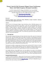
<strong>Reconstruction</strong> <strong>de</strong> <strong>formes</strong> <strong>3D</strong> usinées<br />
<strong>par</strong> stéréocorrélation d’images<br />
à <strong>par</strong>tir d’un modèle CAO<br />
Présentation <strong>de</strong> stage<br />
John-Eric Dufour<br />
Encadré <strong>par</strong> : F. Hild<br />
28 juin 2012
J.-E. Dufour <strong>Reconstruction</strong> <strong>3D</strong> <strong>par</strong> stéréocorrélation 2<br />
Sommaire<br />
1 Motivation <strong>de</strong> l’étu<strong>de</strong><br />
2 Mesure <strong>de</strong>s distorsions optiques<br />
3 <strong>Reconstruction</strong>s <strong>de</strong> forme <strong>3D</strong><br />
4 Conclusion
J.-E. Dufour <strong>Reconstruction</strong> <strong>3D</strong> <strong>par</strong> stéréocorrélation 3<br />
Motivation<br />
Plan<br />
1 Motivation <strong>de</strong> l’étu<strong>de</strong><br />
Rappels <strong>de</strong> corrélation d’images<br />
Algorithme utilisé<br />
2 Mesure <strong>de</strong>s distorsions optiques<br />
Métho<strong>de</strong><br />
Modèle Spline<br />
3 <strong>Reconstruction</strong>s <strong>de</strong> forme <strong>3D</strong><br />
Carreau<br />
Pièce Cylindrique<br />
4 Conclusion
J.-E. Dufour <strong>Reconstruction</strong> <strong>3D</strong> <strong>par</strong> stéréocorrélation 4<br />
Motivation<br />
Contexte<br />
Les techniques <strong>de</strong> corrélation <strong>3D</strong> surfaciques sont <strong>de</strong> plus<br />
en plus développées :<br />
Mesures sans contact<br />
Mise en oeuvre plus rapi<strong>de</strong><br />
Métho<strong>de</strong> autorisant <strong>de</strong>s mesures in situ <strong>de</strong> gran<strong>de</strong>s<br />
pièces<br />
Exemples <strong>de</strong> pièces complexes à mesurer.
J.-E. Dufour <strong>Reconstruction</strong> <strong>3D</strong> <strong>par</strong> stéréocorrélation 5<br />
Motivation<br />
Caractéristiques<br />
(a) Carreau théorique<br />
(b) Carreau réel<br />
Carreau <strong>de</strong> Bézier utilisé comme cas test
J.-E. Dufour <strong>Reconstruction</strong> <strong>3D</strong> <strong>par</strong> stéréocorrélation 6<br />
Motivation Rappels Corrélation<br />
La corrélation d’images consiste à trouver le champ <strong>de</strong><br />
déplacement u qui permet <strong>de</strong> passer d’une image f à une<br />
image g.<br />
On cherche à minimiser la fonction suivante<br />
∫<br />
η 2 = [f(x) − g(x + u(x))] 2 dx (1)<br />
Ω<br />
ce qui revient à résoudre le problème suivant<br />
Ma = b (2)<br />
avec M = ∫ Ω [∂u ∂a ∇f]2 et b = ∫ Ω [∂u ∇f · (g(x) − f(x))]<br />
∂a
J.-E. Dufour <strong>Reconstruction</strong> <strong>3D</strong> <strong>par</strong> stéréocorrélation 7<br />
Motivation Algorithme utilisé CORRELI_ETAL<br />
Étalonnage <strong>de</strong>s matrices <strong>de</strong> passage<br />
Surface fixe<br />
M g<br />
M d<br />
Corrélation<br />
dM g dM d<br />
Auto-étalonnage
J.-E. Dufour <strong>Reconstruction</strong> <strong>3D</strong> <strong>par</strong> stéréocorrélation 8<br />
Motivation Algorithme utilisé CAD_CORRELI_ETAL<br />
Mg fixe<br />
Md fixe<br />
Corrélation<br />
dPij<br />
<strong>Reconstruction</strong> <strong>de</strong> forme
J.-E. Dufour <strong>Reconstruction</strong> <strong>3D</strong> <strong>par</strong> stéréocorrélation 9<br />
Motivation Algorithme utilisé Image distordue<br />
0<br />
200<br />
400<br />
600<br />
800<br />
Residuals scale = 1 Iteration = 1<br />
3<br />
2<br />
1<br />
0<br />
−1<br />
−2<br />
−3<br />
0 200 400 600 800<br />
Résidus <strong>de</strong>s images non corrigées
J.-E. Dufour <strong>Reconstruction</strong> <strong>3D</strong> <strong>par</strong> stéréocorrélation 10<br />
Distorsions<br />
Plan<br />
1 Motivation <strong>de</strong> l’étu<strong>de</strong><br />
Rappels <strong>de</strong> corrélation d’images<br />
Algorithme utilisé<br />
2 Mesure <strong>de</strong>s distorsions optiques<br />
Métho<strong>de</strong><br />
Modèle Spline<br />
3 <strong>Reconstruction</strong>s <strong>de</strong> forme <strong>3D</strong><br />
Carreau<br />
Pièce Cylindrique<br />
4 Conclusion
J.-E. Dufour <strong>Reconstruction</strong> <strong>3D</strong> <strong>par</strong> stéréocorrélation 11<br />
Distorsions Métho<strong>de</strong> Définition<br />
"Définition"<br />
Artefacts optiques dus à l’imperfection <strong>de</strong>s moyens utilisés.<br />
→ décalage systématique <strong>de</strong>s pixels observés.<br />
(a) Radiale (b) Décentrage (c) Prismatique<br />
Exemples <strong>de</strong> distorsions
J.-E. Dufour <strong>Reconstruction</strong> <strong>3D</strong> <strong>par</strong> stéréocorrélation 12<br />
Distorsions Métho<strong>de</strong> Objectifs<br />
Objectif :<br />
Quantifier les distorsions optiques pour un réglage d’ap<strong>par</strong>eil<br />
photo donné<br />
Outils :<br />
On utilise pour cela la corrélation d’images numériques.<br />
Plusieurs solutions :<br />
Utiliser une base riche (Q4,...) puis projeter le résultat<br />
sur les champs <strong>de</strong> distorsions.
J.-E. Dufour <strong>Reconstruction</strong> <strong>3D</strong> <strong>par</strong> stéréocorrélation 13<br />
Distorsions Métho<strong>de</strong> Objectifs<br />
Objectif :<br />
Quantifier les distorsions optiques pour un réglage d’ap<strong>par</strong>eil<br />
photo donné<br />
Outils :<br />
On utilise pour cela la corrélation d’images numériques.<br />
Plusieurs solutions :<br />
Utiliser une base riche (Q4,...) puis projeter le résultat<br />
sur les champs <strong>de</strong> distorsions.<br />
Utiliser directement la base <strong>de</strong>s distorsions pour<br />
effectuer la corrélation.
J.-E. Dufour <strong>Reconstruction</strong> <strong>3D</strong> <strong>par</strong> stéréocorrélation 14<br />
Distorsions Métho<strong>de</strong> Caractéristiques<br />
On utilise une mire pour mesurer les distorsions :<br />
Motif aléatoire mais connu<br />
Com<strong>par</strong>aison entre une photo et la mire numérique<br />
Mires numérique et réelle utilisées pour les mesures
J.-E. Dufour <strong>Reconstruction</strong> <strong>3D</strong> <strong>par</strong> stéréocorrélation 15<br />
Distorsions Métho<strong>de</strong> Base modifiée<br />
Si l’on prend en compte le décalage (X 0 , Y 0 ) <strong>de</strong> l’axe <strong>de</strong>s<br />
distorsions la base <strong>de</strong>s distorsions <strong>de</strong>vient :<br />
axe x<br />
axe y<br />
1 0<br />
0 1<br />
X 0<br />
0 X<br />
Y 0<br />
0 Y<br />
(X − X 0 )((X − X 0 ) 2 + (Y − Y 0 ) 2 ) (Y − Y 0 )((X − X 0 ) 2 + (Y − Y 0 ) 2 )<br />
2(X − X 0 )(Y − Y 0 ) (X − X 0 ) 2 + 3(Y − Y 0 ) 2<br />
3(X − X 0 ) 2 + (Y − Y 0 ) 2 2(X − X 0 )(Y − Y 0 )<br />
(X − X 0 ) 2 + (Y − Y 0 ) 2 0<br />
0 (X − X 0 ) 2 + (Y − Y 0 ) 2<br />
Base <strong>de</strong> fonctions <strong>de</strong> forme modifiée
J.-E. Dufour <strong>Reconstruction</strong> <strong>3D</strong> <strong>par</strong> stéréocorrélation 16<br />
Distorsions Modèle Spline Résultats<br />
On peut également utiliser une décomposition spline pour<br />
écrire les distorsions.<br />
X ( p i x e l )<br />
100<br />
200<br />
300<br />
400<br />
500<br />
600<br />
U x ( p i x e l )<br />
1<br />
0<br />
−1<br />
−2<br />
X ( p i x e l )<br />
100<br />
200<br />
300<br />
400<br />
500<br />
600<br />
U x ( p i x e l )<br />
2<br />
1<br />
0<br />
−1<br />
−2<br />
700<br />
800<br />
900<br />
200 400 600 800<br />
Y ( p i x e l )<br />
−3<br />
−4<br />
700<br />
800<br />
900<br />
200 400 600 800<br />
Y ( p i x e l )<br />
−3<br />
−4<br />
(a) Métho<strong>de</strong> intégrée<br />
(b) Métho<strong>de</strong> spline<br />
Champs <strong>de</strong> déplacements dans la direction X avec <strong>de</strong>ux métho<strong>de</strong>s<br />
différentes.
J.-E. Dufour <strong>Reconstruction</strong> <strong>3D</strong> <strong>par</strong> stéréocorrélation 17<br />
Distorsions Modèle Spline Com<strong>par</strong>atif<br />
X ( p i x e l )<br />
100<br />
200<br />
300<br />
400<br />
500<br />
600<br />
700<br />
800<br />
900<br />
R e s i d u s ( n i v e a u d e g r i s )<br />
250<br />
100<br />
200 200<br />
150<br />
100<br />
50<br />
200 400 600 800<br />
0<br />
Y ( p i x e l )<br />
(a) Métho<strong>de</strong> intégrée<br />
X ( p i x e l )<br />
300<br />
400<br />
500<br />
600<br />
700<br />
800<br />
900<br />
R e s i d u s ( n i v e a u d e g r i s )<br />
250<br />
200<br />
150<br />
100<br />
50<br />
200 400 600 800<br />
0<br />
Y ( p i x e l )<br />
(b) Métho<strong>de</strong> spline<br />
Résidus <strong>de</strong> corrélation pour <strong>de</strong>ux métho<strong>de</strong>s différentes.
J.-E. Dufour <strong>Reconstruction</strong> <strong>3D</strong> <strong>par</strong> stéréocorrélation 18<br />
<strong>Reconstruction</strong> <strong>3D</strong><br />
Plan<br />
1 Motivation <strong>de</strong> l’étu<strong>de</strong><br />
Rappels <strong>de</strong> corrélation d’images<br />
Algorithme utilisé<br />
2 Mesure <strong>de</strong>s distorsions optiques<br />
Métho<strong>de</strong><br />
Modèle Spline<br />
3 <strong>Reconstruction</strong>s <strong>de</strong> forme <strong>3D</strong><br />
Carreau<br />
Pièce Cylindrique<br />
4 Conclusion
J.-E. Dufour <strong>Reconstruction</strong> <strong>3D</strong> <strong>par</strong> stéréocorrélation 19<br />
<strong>Reconstruction</strong> <strong>3D</strong> Carreau Image distordue<br />
0<br />
200<br />
400<br />
600<br />
800<br />
Residuals scale = 1 Iteration = 1<br />
3<br />
2<br />
1<br />
0<br />
−1<br />
−2<br />
−3<br />
0 200 400 600 800<br />
Résidus <strong>de</strong>s images non corrigées
J.-E. Dufour <strong>Reconstruction</strong> <strong>3D</strong> <strong>par</strong> stéréocorrélation 20<br />
<strong>Reconstruction</strong> <strong>3D</strong> Carreau Image corrigée<br />
0<br />
100<br />
200<br />
300<br />
400<br />
500<br />
600<br />
Residuals scale = 1 Iteration = 1<br />
3<br />
2<br />
1<br />
0<br />
−1<br />
700<br />
−2<br />
800<br />
900 −3<br />
0 200 400 600 800<br />
Résidus <strong>de</strong>s images corrigées
J.-E. Dufour <strong>Reconstruction</strong> <strong>3D</strong> <strong>par</strong> stéréocorrélation 21<br />
<strong>Reconstruction</strong> <strong>3D</strong> Carreau Com<strong>par</strong>aison MMT/Stéréo<br />
40<br />
35<br />
30<br />
25<br />
20<br />
15<br />
10<br />
5<br />
10 20 30<br />
(a) Ecart <strong>par</strong> MMT.<br />
RMS = 0.011 mm.<br />
Temps <strong>de</strong> mesure : 4h.<br />
0.045<br />
0.04<br />
0.035<br />
0.03<br />
0.025<br />
0.02<br />
0.015<br />
0.01<br />
0.005<br />
0<br />
80<br />
60<br />
(b) Ecart <strong>par</strong> stéréocorrélation.<br />
RMS = 0.012 mm.<br />
Temps <strong>de</strong> mesure : 2h.<br />
40<br />
20<br />
90<br />
80<br />
70<br />
60<br />
50<br />
40<br />
30<br />
20<br />
10<br />
0.045<br />
0.04<br />
0.035<br />
0.03<br />
0.025<br />
0.02<br />
0.015<br />
0.01<br />
0.005<br />
0<br />
Ecarts mesurés avec les différentes métho<strong>de</strong>s.
J.-E. Dufour <strong>Reconstruction</strong> <strong>3D</strong> <strong>par</strong> stéréocorrélation 22<br />
<strong>Reconstruction</strong> <strong>3D</strong> Pièce Cylindrique Essais sur pièce complexe<br />
Des essais ont été réalisés sur une pièce <strong>de</strong> train<br />
d’atterrissage actuellement développée <strong>par</strong><br />
Messier-Bugatti-Dowty.<br />
Pièce fournie <strong>par</strong> Messier-Bugatti-Dowty.<br />
Sa hauteur est d’environ 500 mm.
<strong>Reconstruction</strong> <strong>3D</strong> Pièce Cylindrique Forme<br />
120<br />
100<br />
80<br />
60<br />
40<br />
20<br />
0<br />
−20<br />
250<br />
200<br />
150<br />
(a) Ecarts à la surface théorique.<br />
RMS = 0.07 mm<br />
100<br />
50<br />
200<br />
150<br />
100<br />
50<br />
1000<br />
2000<br />
3000<br />
4000<br />
Residuals<br />
5000 −45<br />
1000 2000 3000 4000 5000<br />
(b) Résidus <strong>de</strong> corrélation.<br />
Résidu global = 2.98%<br />
Résultats concernant la reconstruction d’un cylindre<br />
30<br />
15<br />
0<br />
−15<br />
−30<br />
Écarts cohérents avec le procédé d’après l’industriel.<br />
J.-E. Dufour <strong>Reconstruction</strong> <strong>3D</strong> <strong>par</strong> stéréocorrélation 23
J.-E. Dufour <strong>Reconstruction</strong> <strong>3D</strong> <strong>par</strong> stéréocorrélation 24<br />
Conclusion<br />
Plan<br />
1 Motivation <strong>de</strong> l’étu<strong>de</strong><br />
Rappels <strong>de</strong> corrélation d’images<br />
Algorithme utilisé<br />
2 Mesure <strong>de</strong>s distorsions optiques<br />
Métho<strong>de</strong><br />
Modèle Spline<br />
3 <strong>Reconstruction</strong>s <strong>de</strong> forme <strong>3D</strong><br />
Carreau<br />
Pièce Cylindrique<br />
4 Conclusion
J.-E. Dufour <strong>Reconstruction</strong> <strong>3D</strong> <strong>par</strong> stéréocorrélation 25<br />
Conclusion<br />
Conclusion<br />
Nous avons développé une nouvelle métho<strong>de</strong> d’étalonnage<br />
<strong>de</strong>s systèmes <strong>de</strong> stéréocorrélation.<br />
Auto-étalonnage à <strong>par</strong>tir <strong>de</strong> la forme théorique observée<br />
<strong>Reconstruction</strong> <strong>de</strong> la forme réelle à <strong>par</strong>tir <strong>de</strong>s images<br />
observées<br />
Nous avons observé les influences <strong>de</strong>s distorsions optiques<br />
sur la reconstruction <strong>de</strong> forme.
J.-E. Dufour <strong>Reconstruction</strong> <strong>3D</strong> <strong>par</strong> stéréocorrélation 26<br />
Conclusion<br />
Perspectives<br />
Mesure <strong>de</strong> <strong>formes</strong> <strong>de</strong> gran<strong>de</strong> taille<br />
Mesure <strong>de</strong> <strong>formes</strong> <strong>3D</strong> <strong>de</strong>s pièces complexes<br />
Pièce complexe difficile à mesurer
J.-E. Dufour <strong>Reconstruction</strong> <strong>3D</strong> <strong>par</strong> stéréocorrélation 27<br />
Conclusion Merci Questions ?<br />
Merci <strong>de</strong> votre attention.<br />
Questions ?
J.-E. Dufour <strong>Reconstruction</strong> <strong>3D</strong> <strong>par</strong> stéréocorrélation 28<br />
Conclusion Merci Paramètres d’usinage<br />
plan <strong>par</strong>allèles<br />
outil boule D20mm<br />
Discrétisation <strong>par</strong> interpolation linéaire<br />
le long d’une passe : tolérance <strong>de</strong> 0.001 mm<br />
entre passe : hauteur <strong>de</strong> crête : 0.001 mm<br />
suivi <strong>de</strong> la trajectoire : Option CN approximation <strong>de</strong>s<br />
segments <strong>par</strong> courbe BSpline <strong>de</strong> <strong>de</strong>gré 3<br />
tolérance <strong>de</strong> suivi <strong>de</strong>s axes <strong>de</strong> 0.05 mm<br />
Repère <strong>de</strong> dégauchissage sur les 4 faces
J.-E. Dufour <strong>Reconstruction</strong> <strong>3D</strong> <strong>par</strong> stéréocorrélation 29<br />
Conclusion Merci Com<strong>par</strong>atif<br />
5.5<br />
Residus en %<br />
5<br />
4.5<br />
Residus Q4<br />
Residus <strong>de</strong> projection<br />
Residus distorsions<br />
4<br />
0 10 20 30 40 50 60 70<br />
Taille d elements<br />
Com<strong>par</strong>aison entre les différentes métho<strong>de</strong>s <strong>de</strong> calcul.
J.-E. Dufour <strong>Reconstruction</strong> <strong>3D</strong> <strong>par</strong> stéréocorrélation 30<br />
Conclusion Merci Com<strong>par</strong>atif<br />
R e s i d u s ( n i v e a u d e g r i s )<br />
100<br />
X ( p i x e l )<br />
200<br />
300<br />
400<br />
500<br />
600<br />
700<br />
50<br />
0<br />
−50<br />
800<br />
900<br />
200 400 600 800<br />
Y ( p i x e l )<br />
−100<br />
Différence entre les résidus <strong>de</strong> corrélation
J.-E. Dufour <strong>Reconstruction</strong> <strong>3D</strong> <strong>par</strong> stéréocorrélation 31<br />
Conclusion Merci Position<br />
Pour bien tenir compte <strong>de</strong> l’axe <strong>de</strong>s distorsions on doit<br />
déterminer sa position.<br />
On remarque que les dérivées <strong>de</strong>s fonctions <strong>de</strong> forme<br />
radiales sont les fonctions <strong>de</strong> forme <strong>de</strong> décentrage. Ainsi on<br />
a :<br />
∂Φ(x,y) ∂Φ(x,y)<br />
u(x −d 1 ,y −d 2 ) = k 1 Φ(x,y)−k 1 d 1 −k 1 d 2<br />
∂x<br />
∂y<br />
(3)<br />
or les expressions <strong>de</strong>s dérivées <strong>de</strong> Φ étant celles <strong>de</strong>s<br />
fonctions <strong>de</strong> forme <strong>de</strong> décentrage. Alors on a :<br />
−k 1 d i = p i (4)
J.-E. Dufour <strong>Reconstruction</strong> <strong>3D</strong> <strong>par</strong> stéréocorrélation 32<br />
Conclusion Merci NURBS<br />
Le formalisme utilisé pour décrire la surface est <strong>de</strong> type<br />
NURBS.<br />
avec<br />
et<br />
N i,m (u) =<br />
S(u,v) = ∑m i=1 ∑ n j=1 N i,m(u)N j,n (v)ω ij P ij<br />
∑ m i=1 ∑ n j=1 N i,m(u)N j,n (v)ω ij<br />
(5)<br />
∀u ∈ [0,1],N i,0 (u) =<br />
{<br />
1 si u i ≤ u ≤ u i+1<br />
0 sinon<br />
(6)<br />
u − u i<br />
N i,m−1 (u) +<br />
u i+m+1 − u<br />
N i+1,m−1 (u)<br />
u i+m − u i u i+m+1 − u i+1<br />
(7)
J.-E. Dufour <strong>Reconstruction</strong> <strong>3D</strong> <strong>par</strong> stéréocorrélation 33<br />
Conclusion Merci Résultats actuels<br />
Concernant la convergence :<br />
0.052<br />
0.051<br />
0.05<br />
0.049<br />
0.048<br />
0.047<br />
0.046<br />
0.045<br />
0.044<br />
0 1000 2000 3000 4000 5000 6000 7000<br />
Com<strong>par</strong>aison d’itérations nécessaires dans divers configurations
J.-E. Dufour <strong>Reconstruction</strong> <strong>3D</strong> <strong>par</strong> stéréocorrélation 34<br />
Conclusion Merci Corps <strong>de</strong> pièce<br />
En reconstruisant le corps <strong>de</strong> la pièce :<br />
reconstruction du corps <strong>de</strong> la pièce.
J.-E. Dufour <strong>Reconstruction</strong> <strong>3D</strong> <strong>par</strong> stéréocorrélation 35<br />
Conclusion Merci Corps <strong>de</strong> pièce<br />
Residuals scale = 1 Iteration = 2<br />
x 10 4<br />
6<br />
100<br />
200<br />
4<br />
300<br />
2<br />
400<br />
500<br />
0<br />
600<br />
−2<br />
700<br />
−4<br />
800<br />
900<br />
100 200 300 400 500 600 700 800 900<br />
Résidus <strong>de</strong> corrélation sur le corps <strong>de</strong> la pièce. Le résidu global<br />
est <strong>de</strong> 13%
J.-E. Dufour <strong>Reconstruction</strong> <strong>3D</strong> <strong>par</strong> stéréocorrélation 36<br />
Conclusion Merci Déplacements <strong>3D</strong><br />
t<br />
M g<br />
M d<br />
Corrélation<br />
dP i j<br />
t+dt<br />
Métho<strong>de</strong> <strong>de</strong> mesure <strong>de</strong>s champs <strong>de</strong> déplacements <strong>3D</strong>