Rivista Italiana di Agrometeorologia Italian Journal of ...

ISSN 1824-8705
Rivista Italiana di
Agrometeorologia
Rivista Italiana di
Agrometeorologia
anno 9 - n. 1 – Ottobre 2004
Periodico quadrimestrale edito
dall’AIAM
Autorizzazione Tribunale di Firenze n.
5221 del 4/12/2002
Poste Italiane s.p.a. - Spedizione in
Abbonamento Postale -
70% - DCB UDINE.
Italian Journal of Agrometeorology
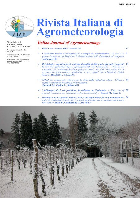
• Aiam News - Notizie dalla Associazione 3
• A Jackknife-derived visual approach for sample size determination - Un approccio
grafico derivato dal jackknife per la determinazione delle dimensioni del campione.
Confalonieri R.
• Metodologie e algoritmi per il controllo di qualità di dati orari e giornalieri acquisiti
da una rete agrometeorologica: applicazioni alle rete lucana SAL - Methods and
algorithms for evaluating the data quality at hourly and daily time scales for an
agrometeorological network: application to the regional net of Basilicata (Italy).
Rana G., Rinaldi M., Introna M.
9
14
• GSRad, un componente software per la stima della radiazione solare - GSRad, a
software component to estimate solar radiation.
Donatelli M., Carlini L., Bellocchi G.
• I fabbisogni idrici del pomodoro da industria in Capitanata - Water use of
processing tomato in the Capitanata region (Southern Italy). Rinaldi M., Rana G.
• Remotely sensed vegetation indices: theory and applications for crop management -
Indici di vegetazione telerilevati: teoria ed applicazioni per la gestione agronomica
delle colture. Basso B., Cammarano D., De Vita P.
24
31
36

Rivista Italiana di Agrometeorologia
Italian Journal of Agrometeorology
Anno 9 - n. 1 – Ottobre 2004
Rivista Italiana di Agrometeorologia
Periodico quadrimestrale edito dall’AIAM
www.agrometeorologia.it
ISSN 1824-8705
EDITORE:
AIAM Associazione Italiana di Agrometeorologia
Presidente: Luigi Mariani
Consiglieri: Maurizio Borin, Andrea Cicogna, Antonino
Drago, Vittorio Marletto, Simone Orlandini, Miriam
Rosini, Emanuele Scalcione.
Revisori dei conti: Federico Spanna, Maria Carmen
Beltrano, Luigi Pasotti
Sede legale - via Caproni 8, 50144 Firenze.
Sede tecnica - via Modigliani 4, 20144 Milano
Direttore responsabile:
Marco Gani - e-mail: marco.gani@csa.fvg.it
Responsabile scientifico (Editor in Chief) :
Maurizio Borin, Dipartimento Di Agronomia Ambientale
e Produzioni Vegetali, Viale dell’Università 16, 35020
Legnaro (Pd), Italy Tel. +39 049 8272838,
e-mail: maurizio.borin@unipd.it
Segretaria di redazione: Roberto Confalonieri
Dipartimento di Produzione Vegetale, Università degli
Studi di Milano, Via Celoria 2, 20133 Milano, Italy
e-mail: roberto.confalonieri@unimi.it
Redazione a cura di: Andrea Cicogna
e-mail: andrea.cicogna@csa.fvg.it
Abbonamenti
La rivista è spedita gratuitamente ai soci Aiam. La quota
associativa all’AIAM per il 2005 è fissata in € 50 per i
soci singoli ed in € 300 per gli enti. I versamenti possono
essere effettuati sul CC postale n. 43686203 intestato ad
Associazione Italiana di Agrometeorologia.
In alternativa il costo dell’abbonamento alla sola rivista è
di € 60 da versare sul medesimo CC postale.
Obiettivi
La Rivista Italiana di Agrometeorologia si propone di
pubblicare contributi scientifici originali, in lingua italiana
ed in lingua inglese, riguardanti l'agrometerologia,
intesa come scienza che studia le interazioni dei fattori
meteorologici ed idrologici con l'ecosistema agricoloforestale
e con l'agricoltura intesa nel suo senso più ampio
e le differenti aree tematiche specifiche di interesse
della disciplina, quali ecofisiologia delle piante erbacee e
arboree, fenologia delle piante coltivate, fitopatologia,
entomologia, fisica del terreno e idrologia, micrometeorologia,
modellistica di simulazione, telerilevamento,
pianificazione territoriale, sistemi informativi geografici
e tecniche di spazializzazione, strumentazione di misura
di grandezze fisiche e biologiche, tecniche di validazione
di dati, agroclimatologia, divulgazione in agricoltura e
servizi di supporto per gli operatori agricoli.
La Rivista si avvale di un Comitato scientifico, che è il
garante della qualità delle pubblicazioni e che per tale
scopo può avvalersi di referee esterni.
Aims
The Rivista Italiana di Agrometeorologia publishes English
or Italian-written original papers about agrometeorology,
that is the science which studies the interactions
between meteorological, hydrological factors and the
agro-forest ecosystem and with agriculture, including all
the related themes: herbaceous and arboreal species ecophysiology,
crop phenology, phytopathology, entomology,
soil physics and hydrology, micrometeorology, crop
modelling, remote-sensing, landscape planning, geographical
information system and spatialization techniques,
instrumentation for physical and biological
measurements, data validation techniques, agroclimatology,
diffusion of information and support services for
farmers.
Submitted articles are reviewed by two independent
members of the Editorial Board or by other appropriate
referees.
Comitato dei referee
(Editorial Board)
M. Acutis, Milano G. Maracchi, Firenze
A. Alvino, Campobasso V. Marletto, Bologna
F. Benincasa, Sassari M. Menenti, Ercolano
M. Bindi, Firenze F. Morari, Padova
S. Bocchi, Milano S. Orlandini, Firenze
M. Borin, Padova A. Pitacco, Padova
A. Brunetti, Roma F. Rossi, Bologna
S. Dietrich, Roma P. Rossi Pisa, Bologna
M. Donatelli, Bologna D. Spano, Sassari
G. Genovese, Ispra
2

Aiam News
Notizie dall’Associazione
E’ NATA RIAm: AUGURI !
Marco Gani – Direttore responsabile
marco.gani@csa.fvg.it
Luigi Mariani – Presidente Aiam
meteomar@libero.it
Non capita tutti i giorni di fondare una
rivista scientifica, intervenendo così
nella genesi di quello che da Galileo in
avanti si è imposto come uno degli ingranaggi
fondamentali della trasmissione
del sapere scientifico. Anche per
questo si deve festeggiare la nascita
della Rivista Italiana di Agrometeorologia
(RIAm), ultimo segno della vitalità
di un’associazione di amici che a
sette anni dalla fondazione mostra di
non aver esaurito la propria spinta propulsiva.
RIAm raccoglie l’eredità di Aiam
News, testata sociale attiva dal 1998 al
2003, ed è il risultato di un progetto in
discussione da circa un biennio e sui
cui obiettivi lasciamo giustamente la
parola al presidente del Comitato
Scientifico prof. Maurizio Borin. Vogliamo
solo rammentare che la rivista
dovrà essere nei prossimi anni uno degli
strumenti chiave per affermare
l’agrometeorologia come disciplina
ponte fra discipline fisiche e biologiche
in una visione complessiva di tipo
agro – ecosistemico.
Il giusto equilibrio fra diverse esigenze
ed aspettative sarà fondamentale per
il futuro del progetto RIAm; pensiamo
in particolare all’equilibrio fra articoli
di ricerca ed articoli a taglio divulgativo
e più legati all’esperienza operativa
dei servizi agrometeorologici. E poiché
tutte le cose viaggiano con le
gambe degli uomini, vogliamo lanciare
un appello perché sia la rivista scientifica
vera e propria (quella per intenderci
sotto la supervisione del Comitato
Scientifico), sia il notiziario non sottoposto
a referaggio siano debitamente
riforniti da parte dei colleghi di articoli
ed informazioni provenienti dal mondo
dei servizi agrometeorologici e dal
mondo della ricerca.
E’ necessario a questo punto sviluppare
qualche considerazione di tipo economico.
La produzione di 250 copie di
una rivista scientifica non è uno scherzo
per i considerevoli costi che comporta.
Per tale ragione il Consiglio Direttivo
ha deciso di aprire la rivista alla
pubblicità e di aumentare le quote sociali
portandole a 50 Euro/anno a partire
dal 2005. Speriamo che queste scelte
siano condivise dai soci e consentano
alla RIAm di prosperare in un quadro
economico di stabilità.
Infine un ringraziamento a tutti coloro
che hanno animato il dibattito che ha
preceduto la genesi di RIAm, al comitato
scientifico ed al suo presidente
Maurizio Borin, agli autori degli articoli
ed infine a chi garantisce
l’indispensabile attività di segreteria
della rivista (Andrea Cicogna e Roberto
Confalonieri).
RIAm: PRIMO NUMERO
Maurizio Borin - Responsabile scientifico
maurizio.borin@unipd.it
Rivista Italiana di Agrometeorologia
nasce con molte ambizioni.
La prima, ovvia, direi istituzionale, è
quella di offrire un’occasione di incontro
e di dialogo fra coloro che, a diverso
titolo, sono attivi in questa affascinante
disciplina: accademici, insegnanti
e ricercatori, tecnici che lavorano nei
servizi, imprese private operanti nella
produzione di tecnologie e nell’ erogazione
di servizi, studi professionali e
consulenti, associazioni di agricoltori e
singoli imprenditori agricoli, organizzazioni
interessate alla gestione ambientale,
studenti, appassionati di vario
genere e quanti altri ancora rivolgano i
loro interessi alle interazioni fra le vicende
atmosferiche e il mondo biologico.
La seconda grande aspirazione è di realizzare
una Rivista veramente multidisciplinare,
che sappia cogliere appieno
lo spirito dell’agrometeorologia.
Anche questo è un obiettivo ambizio-
Preistoria dell’AIAM. Questa foto fu scattata in occasione del primo incontro preliminare alla costituzione dell’associazione, tenutosi a
Milano presso l’Ersal nel febbraio 1996, su invito di Luigi Mariani. In piedi, da sinistra, si riconoscono: Albino Libè, Andrea Pitacco,
Paolo Lega, Sandro Gentilini , Marco Gani, Simone Orlandini, , Marco Bindi, Ezio Bongioni, Massimo De Marziis, Loredana Albano,
Paolo Parati, Umberto Gualteroni, Marina Anelli, Michele Gioletta, Luigi Mariani, Graziano Lazzaroni e Vittorio Marletto. A sedere, da
sinistra, Fernando Antenucci, , Andrea Cicogna, Gaetano Zipoli, Susanna Lessi, Lucio Botarelli, Laura Brazzoli.
3

so, in quanto, in Italia, attualmente,
non tutti i settori scientifici che potrebbero
contribuire al progredire della
materia sono egualmente partecipi ed
attivi. Diviene quindi strategico il
coinvolgimento di esperti e di aree tematiche
che finora sono rimaste un po’
ai margini dell’agrometeorologia, accanto,
ovviamente al rafforzamento dei
contributi provenienti dai settori tradizionali.
Altro traguardo cui ambisce RIAm è di
risultare appetibile sia per ricercatori
che per tecnici. Spesso, infatti, i primi
sono poco interessati a pubblicare in
riviste di carattere divulgativo, mentre
i secondi trovano difficoltà ad apprezzare
i contributi di maggior contenuto
scientifico. L’impostazione data alla
nostra Rivista mira a superare queste
barriere, offrendo una sezione referizzata
a chi vuol vedere validato il proprio
lavoro da un Comitato Scientifico,
ed una di carattere tecnico che dia spazio
ai contributi di carattere prevalentemente
applicativo che rappresentano
comunque un patrimonio imprescindibile
della nostra materia.
Ancora: RIAm ospita lavori sia in italiano
che in inglese e, in tal modo, si
propone anche di richiamare contributi
da oltre confine. Si tratta di una scelta
impegnativa, a mio avviso di grande
rilevanza strategica. La posizione geografica
e politica del nostro Paese offre
grandi potenzialità affinché l’agrometeorologia
italiana divenga un punto di
Il Sito dell’AIAM : www.agrometeorologia.it
riferimento sia per i Paesi del Bacino
Mediterraneo sia per quelli dell’Est
Europeo. In entrambi i casi si tratta di
mondi in grande fermento, che potrebbero
offrire anche notevoli opportunità
di lavoro ed interscambio.
Non va trascurato un altro fondamentale
elemento che vorremmo caratterizzasse
la Rivista: la velocità di pubblicazione.
La dinamicità con cui le
novità scientifiche e tecniche vengono
conseguite, nonché le giuste aspirazioni
di coloro che propongono i loro
contributi, ci spingono ad impegnarci
in un lavoro di revisione serio ma rapido,
in modo da ridurre il più possibile
il tempo che intercorre fra l’invio e
la pubblicazione del lavoro. Proprio in
funzione di questo, RIAm si è data un
Comitato Scientifico di esperti che
hanno aderito entusiasticamente alla
proposta e agli obiettivi: a loro va il
mio sentito grazie.
Ci sarebbero ancora molte altre ambizioni
da ricordare; fra tutte, la piccola
“follia” di uscire in tempi in cui storiche
riviste tecnico-scientifiche del settore
agricolo sono state chiuse o versano
in condizioni di grande difficoltà e
in cui vi è un crescente sviluppo delle
testate pubblicate in internet che competono
con le tradizionali su carta. Anzi,
a tal proposito, ci proponiamo di
sviluppare sinergie fra RIAm e il sito
AIAM (www.agrometeorologia.it).
Questo primo numero nasce come e-
sempio di ciò che si vorrebbe realizzare:
una consistente rassegna bibliografica
su un tema di notevole attualità e
di grande interesse scientifico, quattro
articoli referizzati, svariati contributi
tecnici e segnalazioni di iniziative
dell’Associazione. Un numero vivo,
che ospita già due lavori in inglese,
nello spirito di aprirsi verso tutte le
direzioni.
Mi auguro che la proposta susciti interesse
e che i numeri che seguiranno
siano ancora più ricchi ed accattivanti.
Rivista Italiana di Agrometeorologia
(Italian Journal of Agrometeorology)
is an international journal with the
aim of publishing original articles and
reviews on the inter-relationship between
meteorology and the fields of
plant, animal and soil sciences, environmental
biophysics, ecology, and
biogeochemistry.
This journal has been thought to address
many objectives.
The first, obvious and institutional, is
to offer the chance of meeting and
conversing among all who are actively
involved in this fascinating subject,
each for different reasons: academic
scientists, teachers and researchers,
technicians who work for extension
services, private firms involved in the
production of technologies and supply
of services, professional studies and
consultants, farmers associations and
individual farmers, organizations interested
in environment management,
students, all who are fond of the subject
and all who are interested in the
interactions between the atmospheric
events and the biological world.
The second big aim is to create a truly
multidisciplinary journal, able to fully
catch the spirit of agrometeorology.
This is also an ambitious objective,
because in Italy at this time not all
scientific sectors which could
contribute to the advancement of the
subject are equally present and active.
The involvement of experts and
research areas which have been left at
the margins of agrometeorology is
then crucial, together with the
reinforcement of the contributions
coming from the traditional areas.
Another goal of RIAm (IJAm) is to be
appealing to both researchers and technicians.
Researchers are often not
very interested in publishing on extension
journals, while technicians may
4

find it difficult to appreciate the most
interesting scientific contributions.
Our journal is structured to overcome
these barriers, offering a refereed section
to all who want to see their work
validated by a Scientific Committee,
and a technical section where mostly
applicative and extensions contributions
- that cannot be set aside in our
subject - are welcome.
Moreover, RIAm (IJAm) welcomes papers
both written in Italian and in English,
to draw attention from abroad.
It is a demanding choice, of great strategic
importance in my opinion. The
geographic and political position of
our country offers a great potential for
the Italian agrometeorology to become
a reference point both for the Mediterranean
countries and of the Eastern
Europe countries. Both are worlds
characterized by a great ferment,
which might offer interesting work and
exchange opportunities.
Another fundamental element that will
characterize the journal should not be
neglected: the publishing velocity. The
dynamicity with which scientific news
and techniques are achieved, and the
right aspirations of all who submit
their contributions force ourselves to
commit to a serious but quick revision
work, to reduce as much as possible
the time between the submission and
the publication of the paper. To achieve
this objective RIAm (IJAm) has selected
a Scientific Committee of e-
xperts who have enthusiastically accepted
the invitation and the objectives:
I am deeply thankful to all of
them.
There would still be many other goals
to mention; among all the little “insanity”
to appear at a time when historical
technical-scientific journals of the
agricultural area have been closed or
are going through a critical period
and there is a great development of
journals published on the web, which
compete with the traditional paper
journals. In this regard, we intend to
develop original synergies between
RIAm and the website of the Associazione
Italiana di Agrometeorologia
(www.agrometeorologia.it).
This first number is an example of
what we would like to carry out: a
substantial bibliographic review on a
subject of actual and great scientific
interest, four refereed papers, several
technical contributions and the mention
of all the activities of the Association.
A live number, with two papers in
English, in the spirit of being open to
all directions.
I wish this proposal may be of interest
and that the next numbers will be as
rich and appealing.
CONVEGNO AIAM 2004
Emanuele Scalcione
escalcione@alsia.it
La pressione antropica e le esigenze
legate allo sviluppo economico sottopongono
il territorio e le risorse naturali
ad una pressione e che spesso supera
il limite di sostenibilità dando
luogo a grandi problemi ambientali
che stanno assumendo il carattere della
“globalità” e che rappresentano, nelle
società attuali, gli elementi critici per
lo sviluppo futuro.
Tra questi grandi problemi assumono
rilevanza straordinaria quelli del cambiamento
climatico, della desertificazione
e della biodiversità; si tratta di
temi solo apparentemente separati,
trattandosi, di fatto, di problemi che
richiamano uno stesso argomento di
fondo: lo sviluppo sostenibile delle
popolazioni del pianeta.
E’ in questo contesto che si è inserito
l’appuntamento annuale dell’AIAM a
Matera.
Ovviamente, lo scenario dei Sassi e le
bellissime giornate primaverili hanno
fatto da splendida cornice alle due
giornate di lavoro, risultate assai ricche
di contenuto tecnico e scientifico e che
hanno visto la partecipazione di oltre
un centinaio di persone, per buona parte
provenienti da fuori regione.
Senza dubbio, il tema dell’incontro
“Gli agroecosistemi nel cambiamento
climatico” ha rappresentato un forte
richiamo per la Comunità scientifica e
per i Servizi regionali, in virtù del contributo
che l’agrometeorologia può dare
all’agricoltura su un tema di così
forte attualità.
Le giornate di lavoro hanno dato una
conferma del crescente interesse che
l’AIAM ha creato intorno a sé, rafforzando
il progetto di dar vita, nel prossimo
autunno, alla Rivista Italiana di
Agrometeorologia.
La stessa partecipazione di autorità regionali,
fra gli altri del Presidente della
Giunta Regionale ed il Sindaco di Matera
oltre ad amministratori
dell’ALSIA, ha mostrato l’interesse
che la comunità della Basilicata nutre
nei confronti dell’agrometeorologia e
delle applicazioni di questa disciplina.
A conclusione dei lavori è emerso che
l’agrometeorologia può dare un contributo
di assoluto rilievo allo studio dei
fenomeni in atto con evidenti riflessi
Un momento significativo del convegno: la signora Gabriella Conte ricorda la figura del
marito Michele a cui quest’anno è stato dedicato il premio Aiam per tesi di Laurea in A-
grometeorologia. A fianco della signora il Presidente della Giunta della regione Basilicata
Filippo Bubbico, il Presidente dell’AIAM Luigi Mariani e il Direttore dell'ALSIA Michele
Taranto
5

extra agricoli, visto che l’agricoltura
sta assumendo sempre più un ruolo di
gestione e di conservazione del territorio
e delle risorse naturali.
Infine, un particolare ringraziamento a
tutti coloro che hanno partecipato al
convegno di Matera e quanti hanno
collaborato per la buona riuscita
dell’evento.
IL BOLLETTINO DEL
CENTRO EUROPEO FA 100
Vittorio Merletto
vmarletto@smr.arpa.emr.it
Ogni trimestre, da 25 anni, il Centro
Meteorologico Europeo di Reading,
UK, pubblica il bollettino ECMWF
Newsletter. Come si legge nel numero
100, pubblicato la scorsa primavera, il
bollettino è nato nel 1980, quando il
Centro entrò in piena operatività, cinque
anni dopo la sua fondazione. Si
tratta di un agile fascicolo a colori, ottenibile
gratuitamente scrivendo un
messaggio all’editor Peter White
(P.White@ecmwf.int). Il numero 100
contiene tre articoli tecnico-divulgativi
e numerose notizie. L’articolo più rilevante,
a cura di Frederic Vitart, è intitolato
“Previsioni mensili” e descrive
il sistema sperimentale di previsione
numerica a dieci-trenta giorni realizzato
al Centro europeo per colmare la
lacuna esistente tra il sistema di previsione
a dieci giorni e quello delle previsioni
stagionali, entrambi operativi
presso il Centro. Le previsioni mensili
vengono eseguite due volte al mese e
girano per 32 giorni, con 51 membri,
di cui uno di controllo. Si tratta quindi
di previsioni stocastiche, eseguite con
la tecnica dell’ensemble, in cui il modello
accoppiato oceano-atmosfera,
viene avviato perturbando opportunamente
le condizioni iniziali.
La parte atmosferica consiste nel modello
dell’ ECMWF con risoluzione
orizzontale di circa un grado e 40 livelli
verticali, mentre la parte oceanica
è costituita dal modello HOPE (Hamburg
Ocean Primitive Equation) sviluppato
in Germania.
L’interfaccia tra oceano e atmosfera è
gestita dal sistema OASIS (Ocean,
Atmosphere, Sea-Ice, Soil) di origine
francese. Come scrive suggestivamente
l’autore: “Ogni ora i flussi atmosferici
di quantità di moto, calore e
acqua dolce vengono trasferiti
all’oceano e, in cambio, all’atmosfera
viene passata la temperatura superficiale
dell’oceano”. Questa frequenza
di accoppiamento è ritenuta sufficiente
per seguire lo sviluppo di alcuni sistemi
a scala sinottica, come i cicloni tropicali.
Mentre i dati atmosferici necessari
ad inizializzare la previsione (le
cosiddette “analisi”) sono prontamente
disponibili presso il Centro, i dati oceanici
arrivino con ben dodici giorni di
ritardo, di conseguenza è stato necessario
costruire un sistema per “prevedere”
le condizioni iniziali oceaniche,
integrando il modello del mare a partire
dall’ultima analisi disponibile,
“forzandolo” con dati dalle analisi atmosferiche
disponibili.
L’autore descrive anche la tecnica utilizzata
per contenere la deriva del modello,
che diventa rilevante a partire
dalla seconda settimana di integrazione.
Il sistema di previsione mensile
funziona regolarmente dalla primavera
del 2002 e le sue prestazioni sono interessanti,
almeno fino alla seconda/terza
settimana. Per esempio
l’eccezionale anomalia termica
dell’estate 2003 sull’ Europa centrale,
in particolare i 10 gradi oltre la norma
registrati sulla Francia tra il 3 e il 9
agosto, risultava prevista, anche se
meno intensamente di quanto poi registrato,
almeno da alcuni membri dell’
ensemble, già venti giorni prima
dell’evento stesso. Gli altri articoli si
occupano degli errori sistematici nel
modello del Centro Europeo e della
previsione di onde anomale. Auguri al
bollettino ECMWF per i prossimi 100
numeri.
EMMANUEL LE ROY
LADURIE – HISTOIRE
HUMAINE ET COMPAREE
DU CLIMAT. CANICULES
ET GLACIERS,
XIIIE-XVIIIE SIECLE
(Fayard, pagine 740, 25 euro)
L.Mariani meteomar@libero.it
Con questo suo libro, che vuole essere
il primo tomo di una più ampia storia
umana e comparata del clima, Emmanuel
Le Roy Ladurie attira ancora una
volta l’attenzione del vasto pubblico
sullo stretto legame esistente fra
evoluzione del clima e vita delle società
umane.
Professore al Collège de France, amministratore
generale della Biblioteca
Nazionale (1987-1994), membro
dell’Académie des sciences morales et
politiques, Emmanuel Le Roy Ladurie
è uno fra i maggiori storici francesi
viventi ed è stato fra i primi a parlare
di “storia del clima” con il suo fondamentale
testo del 1967 intitolato Histoire
du climat depuis l'an mil, che ha
avuto una vasta notorietà in Italia nella
traduzione pubblicata da Einaudi
con il titolo Tempo di
festa, tempo di carestia. Storia
del clima dall'anno Mille.
“Je m’en fous comme de l’an
quarante” (me ne frego come
dell’anno quaranta) è
un’espressione idiomatica
francese che trae con ogni
probabilità
origine
dall’inverno 1739-1740. Fu
quello un inverno, racconta
Leroy Ladurie, privo di neve e
marcato da tre mesi di gelate
ininterrotte. All’inverno seguirono
poi una primavera e
un’estate assai piovose che
rovinarono il raccolto dei cereali
dando anche luogo a funeste
inondazioni in gran parte
d’Europa. La stessa vendemmia
fu disastrosa, il che è
un fatto assai meno trascurabile
che oggi, poiché allora il
vino era un genere di prima
6

necessità per un’umanità oppressa dal
lavoro manuale.
Una vera catastrofe dunque, che in
Francia si tradusse in circa 200.000
morti e che bloccò la crescita demografica
francese per almeno un decennio.
Duecentomila morti sono tanti ma senza
dubbio assai meno dei 600.000
morti della grande carestia del 1709 e
del milione di morti provocato dalla
grande carestia del 1693, merito delle
misure di mitigazione basate sull’approvvigionamento
delle zone più
colpite con cereali provenienti da zone
dell’est e dell’ovest della Francia,
meno interessate dal maltempo.
Anche il caldo fu responsabile in passato
di molte vittime: ad esempio le
due estati canicolari del 1718 e 1719
fecero in Francia un totale di 450.000
morti, uccisi dalla disidratazione e dalla
dissenteria.
E che dire poi del legame fra i roghi
delle streghe e il cattivo tempo In
Europa il picco nell’uccisione di
streghe si ha proprio nel periodo compreso
fra 1540 e 1600, proprio nel
culmine della piccola era glaciale. I
roghi interessarono varie parti
d’Europa fra cui Germania, Borgogna,
Inghilterra e Svizzera. Cosa vi è infatti
di più satanico del far cader dal cielo
del ghiaccio in piena estate E così i
roghi per “crimini gelivi” diventavano
rimedi contro grandine o nevicate fuori
stagione. E qui potremmo dire che le
nostre “madonne della neve” hanno
donne della neve” hanno quanto meno
avuto il merito di volgere in positivo
fatti che erano tutt’altro che apprezzati
da popolazioni sempre sull’orlo della
catastrofe alimentare.
E’ evidente, secondo Leroy Ladurie,
che fame ed epidemie derivanti da
cause climatiche sono una chiave di
interpretazione per molte vicende storiche
del passato. Occorre tuttavia procedere
ad un equilibrato dosaggio delle
cause. Se infatti nel XVI secolo le
guerre di religione non hanno in alcun
modo il clima fra le loro cause primarie,
la Lega cattolica non esitò ad imputare
ai politici i cattivi raccolti frutto
di cause climatiche. Si può invece ritrovare
una causa meteorologica primaria
per la Fronda, fenomeno tutto
francese che ebbe origine dai dissesti
finanziari seguiti alla guerra dei
trent’anni ma che trasse forza dai magri
raccolti delle fredde primavere del
triennio 1648-1650.
Da non scordare infine il fatto curioso
per cui il regno del Re Sole fu paradossalmente
marcato da un minimo
d’attività solare, il cosiddetto minimo
di Mounder, che secondo diversi studiosi
è all’origine della piccola era
glaciale.
Approfondimenti
Intervista a Leroy Ladurie di Fabien Gruhier dal
titolo Du climat et des hommes, pubblicata sul
Nouvel Observateur dell’8-14 luglio 2004
(http://www.nouvelobs.com/articles/p2070/a245
630.html)
ULISSE, NELLA RETE
DELLA SCIENZA
Una divulgazione scientifica corretta
ed onesta è merce rara e più che mai
necessaria per affermare le idee di
progresso scientifico ed umano.
Per tale ragione è utile segnalare che è
da tempo attiva su Internet una testa
elettronica con scopi di divulgazione
scientifica e tecnologica; il suo nome è
ULISSE, NELLA RETE DELLA
SCIENZA ed è gestita dalla Scuola
Internazionale Superiore di Studi A-
vanzati (SISSA) di Trieste.
Ulisse pubblica un proprio notiziario
settimanale con approfondimenti su
temi di rilevanza scientifica ed inoltre
risponde alle domande più disparate
che provengono da un pubblico affezionato.
Le risposte sono affidate a e-
sperti nelle più svariate discipline, inseriti
in questo contesto di rete e che
operano a titolo volontario. L’esperto
riceve la domanda e nel caso abbia
tempo e cognizioni sufficienti per rispondere
provvede in tal senso; in caso
contrario passa la palla a qualcun altro.
Fra gli esperti “caduti nella rete” e che
hanno finora contribuito all’attività di
Ulisse con risposte in ambito meteo
climatico ed agrometeorologico ricordiamo
fra gli altri Andrea Cicogna,
Marco Gani, Luigi Mariani e Fulvio
Stel. Ulisse è consultabile all’indirizzo
http://ulisse.sissa.it/
Agrometeorologia, risorse naturali e sistemi di gestione del territorio
8° convegno annuale dell’AIAM
primo annuncio
L’edizione 2005 del Convegno Nazionale dell’Associazione Italiana di Agrometeorologia, dal titolo
“Agrometeorologia, risorse naturali e sistemi di gestione del territorio” si svolgerà in Abruzzo;
l’iniziativa rientra nel programma di Assistenza tecnica dell’ARSSA.
La manifestazione si svolgerà nei giorni 3, 4 e 5 Maggio 2005, e sarà articolata nelle seguenti tre
sessioni:
· Riduzione dell’impatto ambientale
· Sistemi informativi territoriali
· Aree protette
Il Convegno si svolgerà a Vasto nei primi due giorni (3-4 maggio), mentre l’ultima giornata (5 maggio),
dedicata alle aree protette, avrà luogo a S. Eufemia a Maiella, presso la sala Convegni dell’Orto
Botanico del Parco Nazionale della Maiella.
L’organizzazione a livello locale sarà curata dai colleghi Ferdinando Antenucci e Bruno Di Lena.
Per maggiori informazioni è possibile consultare il sito dell’aiam (www.agrometeorologia.it) ovvero
contattare: Bruno Di Lena (bruno.dilena@meteoarssa.abruzzo.it) o Andrea Cicogna (andrea.cicogna@csa.fvg.it)
7

R. Confalonieri - Rivista Italiana di Agrometeorologia 9-13 (1) 2004
Pubblicità sulla Rivista Italiana di Agrometeorologia
In questa Rivista può trovare spazio pubblicità relativa al settore Agrometoerologico.
Condizioni economiche:
- pagina intera 4° di copertina 500 €
- pagina intera – interna 200 €
- modulo minimo: mezza pagina.
- sconto per soci sostenitori dell'AIAM: 10%.
Poichè la ragione sociale dell'Associazione impedisce attività commerciale i fondi saranno introitati a titolo di contributo
e saranno finalizzati alla copertura delle spese di pubblicazione della rivista. Si precisa inoltre che il contributo non è deducibile
dalla dichiarazione IRPEF in quanto AIAM non è una ONLUS.
Le richieste devono essere inviate al presidente dell'Aiam dott. Luigi Mariani (all'indirizzo info@agrometeorologia.it o al
numero telefonico 329/7027077) che è disponibile per ogni ulteriore dettaglio.
Si precisa infine che le richieste che perverranno saranno soddisfatte in ordine di priorità di ricevimento.
8

R. Confalonieri - Rivista Italiana di Agrometeorologia 9-13 (1) 2004
A JACKKNIFE-DERIVED VISUAL APPROACH FOR SAMPLE SIZE
DETERMINATION
UN APPROCCIO GRAFICO DERIVATO DAL JACKKNIFE PER LA DETERMINAZIONE
DELLE DIMENSIONI DEL CAMPIONE
Roberto Confalonieri
Department of Crop Science, Section of Agronomy, University of Milano, Via Celoria 2, 20133 Milano, Italy.
Abstract
The determination of the sample size is one of the most important topics in field research and preliminary sampling sessions
should be carried out to determine the size of the sample before the collection of real data. A new method for sample
size determination is proposed, based on a jackknife visual evolution. The method has been tested to determine (i) the sample
size in a rice field in order to collect aboveground biomass data and (ii) the minimum number of time domain reflectometry
(TDR) data acquisitions necessary to get a reliable estimation of soil water content in a maize field. The 18-plants
sample size determined for rice aboveground biomass with the proposed method is coherent with the 20-plants samples traditionally
harvested for field experiments with rice; while the 8 acquisitions indicated for soil water content take into
account both the effort required for collecting data and the measurement accuracy.
The method does not care if the sample units are normally distributed or not and takes into account both the variation of
accuracy for increasing sample sizes and, indirectly, the effort required for getting the measurements.
Keywords: Monte Carlo, rice, Oryza sativa L., resampling, statistical inference, number of plants, aboveground biomass,
soil water content, TDR
Riassunto
La determinazione delle dimensioni del campione è uno degli aspetti più importanti nella ricerca di campo: sessioni di
campionamento preliminari mirate alla sua valutazione dovrebbero sempre essere condotte prima della raccolta dei dati
veri e propri. In questo lavoro viene proposto un nuovo metodo per la determinazione delle dimensioni del campione, basato
su un evoluzione grafica del jackknife. Il metodo è stato testato (i) per la raccolta di dati di biomassa per la coltura del
riso e (ii) per la determinazione del numero minimo di letture al TDR (time domain reflectometer) necessarie per una stima
affidabile del contenuto idrico del terreno in un campo di mais. La dimensione del campione di 18 piante indicata dal metodo
proposto è coerente con il campione di 20 piante tradizionalmente raccomandato per esperimenti di campo in risaia.
Le 8 acquisizioni al TDR indicate per il contenuto idrico del terreno tengono in considerazione sia lo sforzo necessario per
la raccolta del dato che l’affidabilità della misura.
Il metodo funziona sia per campioni distribuiti normalmente che non e, indirettamente, tiene conto dello sforzo necessario
per ottenere il dato sperimentale.
Parole chiave: Monte Carlo, riso, Oryza sativa L., ricampionamento, inferenza statistica, numero di piante, biomassa,
contenuto idrico del terreno, TDR
Introduction
The determination of the sample size is one of the most
important topics for the collection of reliable measurements
of variables describing plant growth (e.g. aboveground
biomass (AGB), leaf area index) and, in general,
for all the aspects of field research.
In many cases, the classical inferential methods based on
the t distribution for determining the sample size cannot
be used: the characteristics of the population (µ and σ)
are unknown. They varies according to many factors
(e.g. homogeneity of the incorporation of residues, of
Corresponding author. tel. +39 02 5031 6592
fax +39 02 5031 6575
e-mail address: roberto.confalonieri@unimi.it (R.Confalonieri).
sowing, of germination, of emergence, etc.). For these
reasons, it is impossible to have a presumptive knowledge
of the sampling error that can be accepted for the
calculation of the sample size: it could change from an
experimental field (or situation) to another. For this reason,
it is better to analyze the trend of the relative variability
inside the same field when the sample size increases
rather than assuming absolute criterions for the acceptance
of a specific variability for the determination of
the sample size. In this way, the effort required for
processing a sample can be easily taken into account too.
Moreover, a reliable evaluation of the fact that the population
is normally distributed is often not possible because,
above all for time-consuming or costly methods, only

R. Confalonieri - Rivista Italiana di Agrometeorologia 9-13 (1) 2004
few observations can be determined in the preliminary
study carried out for determining the sample size.
It is possible to find in the Literature examples of alternative
methods for sample size determination. Wolkowski
et al. (1988), in an experiment aiming at comparing
field plot techniques for corn grain and dry matter yield
estimation, determined the sample size by harvesting all
the plants belonging to a row and determining AGB on
1, 5, 10, 15, 20, 25, all plants of the row randomly e-
xtracted from the whole harvested plants and calculating
the coefficient of variation [CV = standard deviation (average
value) -1 ] of each sample. They found that the coefficient
of variation minimizes for 10 and 15 – plants
samples. The samples extracted from the same row can
not be considered completely independent. Moreover,
the Authors don’t specify if the plants belonging to a
sample had been used to determine the AGB of other
samples.
It’s possible to find in the Literature studies for rice sample
size (= number of plants) determination, although
they were not directly related to AGB determination. For
example, Tirol Padre et al. (1988), in an experiment a-
bout acetylene reduction activity in different rice varieties,
noticed that the average CV (computed from the different
varieties CV, obtained from many measurement
replicates) decreased from 33% with 1 plants to 11% for
6 plants. The Authors discussed that, for some samples,
the variances were correlated to the means (nothomoscedastic)
and for others not (homoscedastic). For
these reason, probably the CV is not the better parameter
for sample size determination: it should be more correct
the separated analysis of means and standard deviations.
A different approach, based on the different components
of the effort required for the whole process to determine
an experimental value, was proposed by Yonezawa
(1985) to determine the minimum number of plants required
for the conservation of plant genetic resources.
The Author concluded that (i) a sample size as small as
10 plants per site or population is reasonable to cover a
large target area and (ii) it is more important to analyze a
wide number of site or population. This conclusion could
be extendable to an experimental field by considering,
for example, the sites corresponding to the plots per
treatment. In this way, it’s possible to conclude that, for
the same available effort, it’s better to harvest few plants
per plot but dispose of more plots for each treatment.
From the 60s resampling methods are increasingly diffused
in biological and environmental sciences. They conceptually
derive from the “Monte Carlo” methods, for
the first time applied to a physical process by Barker
(1965) but they are based on the repeated use of the data
from the same sample (the only one sample which has
been collected). Efron and Tibshirani (1991) underline
the enormous potentiality of these techniques, which widely
use the calculation capability of computers, for the
research on inferential statistics. The bootstrap (Efron,
1979; Efron and Tibshirani, 1993) and the jackknife
(Quenouille, 1949; Tukey, 1958) are particularly important,
both because they are increasingly used and because
of the number of studies and developments they generated.
Therefore, the objectives of this study are (i) the development
of an alternative method for sample size determination
based on an evolution of the jackknife; (ii) its evaluation
for determining the sample size for aboveground
biomass in a rice field and for soil water content in a
maize field. In the first case the sample size will be determined
as number of plants and, in the second, as number
of TDR (Time Domain Reflectometer) measurements.
Materials and methods
Experimental data
Experimental data were collected in 2 experiments. The
first was carried out in Besate (northern Italy, latitude
45° 18’ N, longitude 8° 58’ E) during 2003. Rice (Oryza
sativa L; cv. Volano) was sown in April 28 and grown
under flooded conditions. No water stresses were observed
during the crop cycle and the management has
allowed to prevent the presence of weed and pests. During
this experiment, the studied variable was aboveground
biomass. The samples were collected when the
plants were young (3 leaves) and the dry weight of each
plant was very low. For this reason, we have chosen to
use a group of 3 plants as sampling unit instead of a single
plant in order to avoid errors due to the measurement
of very small quantities of biomass.
The second experiment was carried out in Lodi Vecchio
(northern Italy, latitude 45° 19’ N, longitude 9° 26’ E)
during 2004. Maize (Zea mais L) was grown under optimal
water and nutrients availability. The soil is a Ultic
Haplustalfs fine silty, mixed, mesic (Soil Survey Staff,
1999), subacid, with medium organic matter content, sufficient
available phosphorous and medium potassium
content. The studied variable was soil water content. In
this case, the sampling unit was a single TDR (Time
Domain Reflectometer) measurement event.
A visual jackknife evolution for determining
the sample size
The proposed method can be considered a modification
of the jackknife, developed by Tukey (1958) at the end
of the 50s on the basis of an idea of Quenouille (1949;
1956) of some years before and reviewed, with its recent
developments, by Hinkley (1983).
According to this technique, the original sample of N
elements is divided into groups of k elements. If N is
low, k may be equal to 1. N!
virtual samples
( N − k) ! k!
(combinations without repetitions) of (N-k) elements are
generated by eliminating N!
times k different values
from the original sample. Mean, standard deviation,
( N − k) ! k!
etc. can be calculated for all the generated virtual samples.
In the presented method, different values of k are used.
The process of generation of the N!
virtual samples
is repeated (N-1) times with k assuming values
( N − k )!
k !
from
10

R. Confalonieri - Rivista Italiana di Agrometeorologia 9-13 (1) 2004
1 to (N-2), for a total of
N ! different virtual
N
∑ − 2
k = 1 ( N − k )!
k!
samples.
Mean and standard deviation are computed for all the
generated samples and plotted on two charts, with the
values of (N-k) on the X-axis (Figures 1 and 2) and the
means (or standard deviations) on the Y-axis, in order to
get a visual representation of how the means and the
standard deviations of the generated samples vary with
increasing sample size.
Analyzing the trends of the means and the standard deviations
for increasing values of (N-k), the sample size is
considered equal to the (N-k) value for which the variability
among the means and the standard deviations
computed for almost all the generated samples changes
its decreasing rate, assuming a slow – asymptotic trend
for increasing (N-k) values. This change of rate can be
determined by the observation of how the variability
among means and standard deviations evolves for increasing
(N-k) values or by using an automatic algorithm.
In the second case, the following procedure is
adopted:
1. select a (N-k) value (N-k)’ higher than 2 and lower
than N-2;
2. for i from 2 to (N-k)’, calculate mean and standard
deviation of the 5% highest means (respectively Y i and
s i );
3. compute a linear regression weighted on the standard
deviations assuming as independent variable the
(N-k) values and as dependent one the Y i values and
computing the R 2 of the regression (R 2 _1);
4. repeat the steps [2] and [3] for the 5% lowest means,
determining R 2 _2;
5. for i from (N-k)’ to N-1, repeat the steps from [2] to
[4] to compute R 2 _3 and R 2 _4, imposing that the slope
of the regression is 0;
6. calculate SR 2 by adding R 2 _1, R 2 _2, R 2 _3 and R 2 _4;
7. repeat the steps from [2] to [6] for each of the (N-k)’
values higher than 2 and lower than N-2;
8. the automatically determined sample size based on
the means (AM) is the (N-k)’ value corresponding to
the lower SR 2 .
The same procedure is used to determine the sample size
basing on the standard deviations (ASD). The highest
between AM and ASD is the automatic sample size.
Two important features of the presented method for the
sample size determination are: (i) the initial sample may
be constituted both by independent and not-independent
data and (ii) the data may be both normally or notnormally
distributed. Moreover, it supplies a visual,
easy-to-analyze representation of a particular sample size
directly related to its variability and to the variability of
bigger and smaller samples sizes. In this way, it is easier
to consider the problem of sample size determination
both from the statistical point of view and from the point
of view of the available effort for carrying out the experimentation.
Application of the proposed method for determining the
sample size
For the first experiment, AGB of 12 3-plants samples (36
plants; aggregated sample of 3 sub-samples) was measured.
250 dispositions without repetitions were generated
through a randomization process using the 12 samples.
Only 250 dispositions were randomized because, when
the initial sample is not numerous, an increase of the resamplings
number does not correspond to an effective
improvement of the estimation (Manly, 1991). The obtained
values were collected in a matrix (Matrix O; 12
rows; 250 columns) with the dispositions in the columns
and the values of each disposition in the rows. A new
matrix was created (Matrix M; 11 rows; 250 columns)
and, for each of its columns, the mean value computed
on the first 2 elements of correspondent column of the
Matrix O was stored in the first row; the mean value
computed on the first 3 elements in the second rows and
so on. The same procedure used to create the Matrix M
was followed to create a Matrix SD, containing the standard
deviations of the values stored in the Matrix O.
Therefore, the elements of Matrix M and Matrix SD are
computed by using the following equations.
n
∑ MatrixOij
i=
MatrixM
nj
= 1
n
n
2
⎛
⎞
⎜
MatrixO
n ∑
ij
⎟
⎜
i=
1
∑ MatrixOij
−
⎟
⎜
i=
n ⎟
1
⎜
⎟
MatrixSD
⎝
⎠
nj
=
n
where j indicates the dispositions and n is equal to (N-k).
The elements of Matrix M and Matrix SD were plotted
separately with the 250 series corresponding to the columns
of the two matrixes (Figure 1 and 2).
The same procedure was followed for determining the
sample size (number of TDR measurement events) for
soil water content determination (second experiment).
The only two differences are that the sampling unit was a
single TDR data acquisition instead of an aggregated
sample of 3 plants and that N was, in this case, 18 instead
of 12 (Figure 3 and 4).
Jack: a software for sample size determination using the
visual jackknife
A software was created for the application of the proposed
method (Figure 5). It generates the virtual samples
and the matrixes of the means and of the standard deviations.
It produces the relative diagrams, draws the 4 regression
lines used by the automatic method for sample
size determination and compute the CV obtainable with
the automatic method. It gives to the user the possibility
of choosing different sample sizes allowing him to compare
the CVs obtainable with the two methods (automatic
or not). The software is free downloadable at the
web site:
http://users.unimi.it/agroecol/confalonieri.php.
11

R. Confalonieri - Rivista Italiana di Agrometeorologia 9-13 (1) 2004
12.80
12.20
11.60
11.00
10.40
9.80
2 3 4 5 6 7 8 9 10 11
Sample size
Fig. 1 – Aboveground biomass (rice) - Means of the generated
populations when the jackknife is applied for different k
values. (N-k) values on the X-axis, with k from (N-2) to
1. More details in the text. k is the number of observations
not used by the jackknife; N is the total number of
observations
Fig. 1 - Biomassa aerea (riso) - Medie delle popolazioni generate
applicando il jackknife per differenti valori di k.
Sull’asse delle X i valori (N-k), con k da (N-2) a 1.
Maggiori dettagli nel testo. k è il numero di osservazioni
non utilizzate nel jackknife; N è il numero totale di osservazioni
25.00
23.80
22.60
21.40
20.20
19.00
2 3 4 5 6 7 8 9 10 11 12 13 14 15 16 17
Sample size
Fig. 3 – Soil water content - Means of the generated populations
when the jackknife is applied for different k values.
(N-k) values on the X-axis, with k from (N-2) to 1. More
details in the text. k is the number of observations not u-
sed by the jackknife; N is the total number of observations.
Fig. 3 - Contenuto idrico del terreno - Medie delle popolazioni
generate applicando il jackknife per differenti valori di k.
Sull’asse delle X i valori (N-k), con k da (N-2) a 1. Maggiori
dettagli nel testo. k è il numero di osservazioni non
utilizzate nel jackknife; N è il numero totale di osservazioni
2.60
2.08
1.56
1.04
0.52
4.50
3.60
2.70
1.80
0.90
0.00
2 3 4 5 6 7 8 9 10 11
Sample size (3-plants groups)
0.00
2 3 4 5 6 7 8 9 10 11 12 13 14 15 16 17
Sample size
Fig. 2 – Aboveground biomass (rice) - Standard deviations of
the generated populations when the jackknife is applied
for different k values. (N-k) values on the X-axis, with k
from (N-2) to 1. More details in the text. k is the number
of observations not used by the jackknife; N is the total
number of observations
Fig. 2 - Biomassa aerea (riso) - Deviazioni standard delle popolazioni
generate applicando il jackknife per differenti
valori di k. Sull’asse delle X i valori (N-k), con k da (N-2)
a 1. Maggiori dettagli nel testo. k è il numero di osservazioni
non utilizzate nel jackknife; N è il numero totale di
osservazioni
Fig. 4 – Soil water content - Standard deviations of the generated
populations when the jackknife is applied for different
k values. (N-k) values on the X-axis, with k from (N-
2) to 1. More details in the text. k is the number of observations
not used by the jackknife; N is the total number
of observations.
Fig. 4 - Contenuto idrico del terreno - Deviazioni standard delle
popolazioni generate applicando il jackknife per differenti
valori di k. Sull’asse delle X i valori (N-k), con k da
(N-2) a 1. Maggiori dettagli nel testo. k è il numero di osservazioni
non utilizzate nel jackknife; N è il numero totale
di osservazioni
Fig. 5 – Jack: a software for the visual-jackknife application (http://users.unimi.it/agroecol/confalonieri.php). User’s interface
Fig 5 - Jack: un software per l’applicazione del visual-jackknife (http://users.unimi.it/agroecol/confalonieri.php). Interfaccia utente
12

R. Confalonieri - Rivista Italiana di Agrometeorologia 9-13 (1) 2004
Results and discussion
Aboveground biomass
Figure 1 shows that the differences between the means of
the generated populations, obtained with the proposed
method, decrease for sample size equal to (6×3) plants.
These differences continue to slightly decrease with
higher sample sizes but 6 groups of three plants can be
considered a satisfactory compromise between the effort
to get the measure and its reliability. In fact, although the
differences between the average values decrease also for
sample sizes higher than the indicated one, there is a
clear change in the height of the region of the plot engaged
by the 250 series.
The same considerations can be discussed for Figure 2
(standard deviations of the generated populations). It’s
possible to notice that the height of the region of the plot
engaged by the 250 series is almost constant for sample
sizes higher than 6 group of 3 plants, while higher difference
in standard deviations can be observed considering
less than 18 plants. In practice, a higher number of plants
would increase the effort required by the measurement
without a comparable increase in the accuracy.
In this example, the sample size was determined by
graphically analyzing the two diagrams. This “visual”
procedure allows to determine sample sizes which take
into account the effort required to get data and the experimenter’s
judgement.
Soil water content
For the determination of the number of TDR measurement
events required to get a reliable soil water content
estimation, the automatic procedure was used (see the
section “Materials and methods”).
Figure 3 and 4 show, respectively, the means and the
standard deviations of the generated populations. The
grey straight lines represent the linear regressions on
which the R 2 are computed. The intersection between the
oblique lines and the horizontal ones represents the
automatically computed samples size, also indicated by
the vertical series of dots. It is possible to notice that the
automatically computed sample size is 7 in Figure 3
(means) and 8 in Figure 4 (standard deviations). In this
kind of cases, the proposed algorithm advise to chose the
highest.
The used algorithm has been planned to reproduce the
behavior of an experimenter in selecting a sample size
and it is particularly useful when the area of the diagrams
engaged by the generated series decreases, for increasing
sample sizes, too regularly to allow the experimenter to
confidently notice discontinuities.
Conclusions
When parametric modelling and theoretical analysis are
difficult, the bootstrap (Efron, 1979; Efron and Tibshirani,
1993) and the jackknife (Quenouille, 1949; Tukey,
1958) are good alternatives for analyzing the characteristics
of a population (Park and Willemain, 1999).
The proposed method, based on a visual evolution of the
jackknife has shown to be reliable for sample size determination,
determining sample sizes of (i) 18 plants (6
aggregated samples of 3 plants) for rice aboveground
biomass determination and (ii) 8 TDR measurement e-
vents for soil water content estimation in a maize field.
The first value is coherent with the 20 plants per plot recommended
to be harvested by Gomez (1972) in his manual
about field experiments with rice and traditionally
used in field experiments.
Future studies will evaluate the applicability of the proposed
method to other variables (e.g. leaf area index, soil
nitrogen content, etc).
References
Barker, A.A., 1965. Monte Carlo calculations of the radial distribution
functions for a proton-electron plasma. Australian
Journal of Physics, 18, 119-133.
Efron, B., 1979. Bootstrap methods: another look at the jackknife.
Annals of statistics, 7, 1-26.
Efron, B., Tibshirani, R., 1991. Statistical data analysis in the
computer age. Science, 253, 390-395.
Efron, B., Tibshirani, R., 1993. An introduction to the bootstrap.
Chapman & Hall, New York.
Gomez, K.A., 1972. Techniques for field experiments with rice:
layout, sampling, sources of error. International Rice Research
Institute, Los Baños, Philippines, pp. 46.
Hinkley, D.V., 1983. Jackknife methods. Encyclopedia of Statistical
Science, 4, 280-287.
Manly, B.F.J., 1991. Randomization and Monte Carlo Methods
in Biology. Chapman and Hall, London, New York, USA, pp.
281.
Park, D., Willemain, T.R., 1999. The threshold bootstrap and
threshold jackknife. Computational Statistics & Data Analysis,
31, 187-202.
Quenouille, M.H., 1949. Approximate tests of correlation in
time series. Journal of The Royal Statistical Society, Series B,
11, 68-84.
Quenouille, M.H., 1956. Notes on bias in estimation. Biometrika,
43, 353-360.
Soil Survey Staff, 1999. Soil Taxonomy, 2nd edition. Agric.
Handbook n. 436, USDA-NRCS, 869 pp.
Tirol Padre, A., Ladha, J.K., Punzalan, G.C., Watanabe, I.,
1988. A plant sampling procedure for acetylene reduction assay
to detect rice varietal differences in ability to stimulate
N2 fixation. Soil Biology and Biochemistry, 20, 175-183.
Tukey, J.W., 1958. Bias and confidence in not quite large samples
(Abstract). Annals of Mathematical Statistics, 29, 614.
Wolkowski, R.P., Reisdorf, T.A., Bundy, L.G., 1988. Field plot
technique comparison for estimating corn grain and dry matter
yield. Agronomy Journal, 80, 278-280.
Yonezawa, K., 1985. A definition of the optimal allocation of
effort in conservation of plants genetic resources with application
to sample size determination for field collection. Euphytica,
34, 345-354.
13

G. Rana et al.- Rivista Italiana di Agrometeorologia 14-23 (1) 2004
METODOLOGIE E ALGORITMI PER IL CONTROLLO DI QUALITÀ DI DATI
ORARI E GIORNALIERI ACQUISITI DA UNA RETE AGROMETEOROLOGICA:
APPLICAZIONI ALLE RETE LUCANA SAL
METHODS AND ALGORITHMS FOR EVALUATING THE DATA QUALITY AT HOURLY AND DAILY TIME
SCALES FOR AN AGROMETEOROLOGICAL NETWORK: APPLICATION TO
THE REGIONAL NET OF BASILICATA (ITALY)
Gianfranco Rana*, Michele Rinaldi, Michele Introna
Istituto Sperimentale Agronomico, Via C. Ulpiani, 5 70125 Bari Italy
Riassunto
In questo lavoro sono esaminate le tecniche che si dovrebbero utilizzare per effettuare un controllo di qualità di grandezze
agrometeorologiche acquisite in campo da stazioni standard. Primo passo necessario è calibrare periodicamente i sensori,
per calcolarne i moltiplicatori. Qui, inoltre, sono stati descritti i metodi e gli algoritmi che si utilizzano per i controlli fisici e
formali che hanno come obiettivo quello di determinare se un dato è accettabile; poi si è descritto brevemente il metodo da
utilizzare per costruire l’algoritmo necessario a ristabilire l'integrità dei dati quando uno di essi è stato dichiarato inaccettabile.
I metodi descritti sono stati applicati ad un caso reale: una serie di dati acquisiti dalla rete agrometeorologica della regione
Basilicata. I risultati mostrano che, se viene effettuata periodicamente una calibrazione corretta, i valori non risultano
affetti da un errore significativo e risultano di qualità accettabile per le applicazioni pratiche.
Parole chiave: controlli fisici, controlli statistici, rete agrometeorologica, calibrazione dei sensori, errore.
Abstract
In this paper the techniques to be used for the quality control of standard agrometeorological measurements are studied.
First, it is necessary to calibrate periodically the sensors, in order to compute the conversion coefficients. Furthermore, the
methods and algorithms used for the physical and statistical controls are detailed here, in order to determine if the data
are correct; moreover, a short discussion on the subject of replacing incorrect data by a suitable value is carried out. The
methods described have been applied to a series of data acquired by the local agrometeorological network of Basilicata
(Southern Italy). The results showed that if a correct periodical calibration has been made periodically, the errors affecting
the data are small, at least for practical applications.
Keywords: physical controls, statistical controls, agrometeorological network, sensor calibration, error.
Introduzione
Partiamo dal presupposto che: è meglio non prendere in
considerazione un cattivo dato che tenerne conto in ogni
caso. Infatti, se si prende per buono un dato che buono
non è, si commette senz'altro un errore molto maggiore
di quello che si commetterebbe considerando un dato
"medio", magari ricavato dalla serie storica (anche limitata
nel tempo) della stazione. Per cui, prima di utilizzare
un valore misurato da un sensore, è necessario controllarne
l'integrità e la correttezza, in altre parole è necessario
effettuare un controllo sulla sua qualità (WMO,
1983a).
Se poi un dato climatico affetto da errore sistematico
viene utilizzato in un modello matematico, ciò può portare
ad errori, anche molto consistenti, sul risultato finale
del modello. Per dare un’idea dell'ordine di grandezza
*Corresponding author. tel. +39 080 5475011
fax +39 080 5475023
e-mail: g_rana@libero.it (G.Rana).
14
degli errori che si possono commettere facciamo un e-
sempio: supponiamo di dover calcolare l'evapotraspirazione
di riferimento (ET 0 ) con il modello di Penman-
Monteith (Allen et al., 1998); questo modello richiede
misure di temperatura e umidità dell'aria, velocità del
vento e radiazione solare globale. Se si suppone di commettere
un errore sistematico di +2 °C sulla temperatura
l'errore finale sull’ET 0 nel periodo irriguo estivo (giugno,
luglio e agosto) è di ben 40 mm, ovvero di 400 m 3 /ha di
acqua. I dettagli relativi a questo esempio sono riportati
in Tabella 1; nella stessa tabella è anche presentato
l’effetto sull’ET 0 di un errore sistematico di 10 punti percentuali
nell’umidità relativa dell’aria.
Se il dato dovesse risultare errato anche dopo i controlli
descritti nel seguito, sarà necessario sostituirlo con un
valore appropriato, perché la serie storica resti integra e/o
perché possano essere effettuate tutte le operazioni previste
con quel dato.

G. Rana et al.- Rivista Italiana di Agrometeorologia 14-23 (1) 2004
Si presuppone ovviamente che il valore misurato provenga
da un sensore opportunamente calibrato secondo i
procedimenti indicati in WMO (1981; 1983b). Le modalità
di calibrazione sono descritte in un paragrafo successivo.
Il controllo di qualità dei dati agrometeorologici va fatto
in due momenti distinti (SIAN, 1990): prima si effettuano
dei controlli formali o fisici (controllo sulla accettabilità
generale del dato), poi si eseguono dei controlli
statistici, basati sia sull'analisi delle serie storiche sia sul
controllo dei dati provenienti da stazioni limitrofe.
Dal punto di vista operativo, si procede per i seguenti
due passi:
1) Controlli fisici e formali per determinare se un dato
è accettabile;
2) Adozione di un opportuno algoritmo per ristabilire
l'integrità del dato quando esso è stato dichiarato i-
naccettabile.
I controlli statistici, dettagliati in successivi paragrafi,
devono far riferimento sia al clima della zona interessata,
sia ai dati misurati nei giorni precedenti, sia alle misure
effettuate dalle stazioni limitrofe. In sintesi, si effettuano
i seguenti controlli (SIAN, 1990):
a) controllo sulla variabilità interannuale (clima);
b) controllo sulla persistenza temporale (dati rilevati
nei giorni precedenti);
c) controllo sulla coerenza spaziale (dati rilevati nelle
stazioni limitrofe).
Un discorso a parte merita il problema della standardizzazione
dei dati agrometeorologici, ovvero il controllo
della uniformità dei sensori utilizzati e delle condizioni
ambientali in cui la misura è stata effettuata, ovvero la
valutazione del sito in cui il dato è stato rilevato.
La calibrazione dei sensori per confronto
Per la calibrazione dei sensori e la verifica della loro
funzionalità si seguono le indicazioni dell'Organizzazione
Meteorologica Mondiale (OMM), in particolare, le
procedure standard indicate nei documenti ufficiali
WMO-no. 49 (1988 e successive modifiche e integrazioni),
WMO-no. 134 (1981 e successive modifiche e
integrazioni) e WMO-no. 8 (1983).
La calibrazione di routine viene effettuata per confronto,
ovvero mettendo in relazione i dati provenienti dalla stazione
sotto controllo con quelli acquisiti da una stazione
dotata di sensori di classe di precisione superiore
(Schwerdtfeger, 1976). Nel caso della rete del Servizio
Agrometeorologico Lucano (SAL) sono stati calibrati i
sensori relativi alle seguenti grandezze: radiazione solare
globale, temperatura dell'aria, umidità relativa, velocità
del vento, bagnatura fogliare. Le misure sono state effettuate
con le stesse modalità di acquisizione della rete
SAL.
Da una breve analisi di serie storiche di dati agrometeorologici
relative ad alcune località della regione Basilicata
(vedi Tab. 2), é risultato che il periodo di confronto
ottimale tra stazione di calibrazione e stazione in osservazione
è di circa una settimana. In alcuni casi, dopo
l'immediata analisi dei dati, si è proceduto a prolungare
la calibrazione per confronto fino ad una ulteriore settimana.
La calibrazione per confronto fornisce i due coefficienti
(s e i), rappresentanti la pendenza e l'intercetta della regressione
lineare:
M rif
= s ⋅ M + i
(1)
dove M rif rappresenta la misura effettuata dal sensore di
riferimento e M la misura effettuata con il sensore della
stazione. I due coefficienti vanno poi utilizzati per correggere
i dati provenienti dalle stazioni.
Tab. 1 - Errori totali commessi sull'evapotraspirazione di riferimento
mensile calcolata con il modello di Penman-
Monteith, supponendo di commettere errori sistematici
sulla misura della temperatura dell'aria (T) e dell'umidità
relativa dell'aria (UR).
Tab. 1 - Total errors on the reference evapotranspiration
computed by the Penman-Monteith model, supposing
that constant errors have been made on the measurements
of air temperature (T) and relative humidity (UR).
Errore giugno luglio agosto Totale
2 °C (T) 10 mm 20 mm 10 mm 40 mm
10% (UR) 15 mm 25 mm 15 mm 55 mm
Applicazioni alla rete SAL
Nel periodo maggio 2000-ottobre 2001 sono state calibrate
le 39 stazioni SAL riportate in Tabella II (tra parentesi
la sigla di codifica della stazione).
I sensori presenti nelle stazioni SAL sono di tipo standard,
di differenti case costruttrici e modello, alcuni non
largamente commercializzati. Vista, dunque, la loro
grande varietà si preferisce fornire solo l’intervallo di
precisione in cui cadono tutti i sensori analizzati, per o-
gni grandezza fisica considerata.
- Radiazione solare globale, ±1% - ±3% del fondo
scala.
- Temperatura dell'aria, ±0.5 °C.
- Umidità relativa, ±5 - ±10% del fondo scala.
- Velocità del vento, ±5% del fondo scala, minimo 0.5
m s -1 soglia di avvio.
- Bagnatura fogliare, precisione ±7 - ±10 % del fondo
scala.
Le caratteristiche metrologiche dei sensori utilizzati per
la calibrazione sono qui di seguito riportate.
- Radiazione solare globale, sensore Eppley PSP di
classe I (Fritschen e Gay, 1979), linearità ±0.5% del
valore di fondo scala, tempo di risposta 1 s, sensibilità
9 µV W -1 m 2 .
- Temperatura dell'aria, sensore Rotronic MP 101,
precisione ±0.3 °C, tempo di risposta 15 s.
- Umidità relativa, sensore Rotronic MP101, precisione
±1% del fondo scala, stabilità

G. Rana et al.- Rivista Italiana di Agrometeorologia 14-23 (1) 2004
- Velocità del vento, sensore Met One 010C, precisione
±1% del fondo scala,soglia di avvio,0.27 m s -1 .
- Bagnatura fogliare, sensore Campbell Sci. Mod.
237, precisione ±5% del fondo scala.
In Tabella 3 sono indicati i giudizi complessivi dati alle
stazioni, seguendo i suggerimenti dell’OMM, il significato
del giudizio sintetico è il seguente:
A - sito rappresentativo, stazione in buona posizione
(standard), sensori opportunamente disposti;
B - sito rappresentativo, stazione in posizione accettabile
ma migliorabile (quasi standard), posizione dei sensori
da ottimizzare;
C - sito non rappresentativo, stazione in posizione non
standard, consigliabile lo spostamento.
Per illustrare i risultati e presentare i principali problemi
incontrati, i dati del confronto (tra sensori da calibrare e
sensori di riferimento (rif)) sono illustrati per alcuni sensori
nelle Figure 1-10. Qui di seguito è riportato il commento
e le osservazioni alle figure.
Tab. 2 - Elenco delle stazioni della rete SAL calibrate e loro
ubicazione; in parentesi le sigle.
Tab 2 - List of the calibrated stations of the SAL network and
them site; in brackets the short name.
Tab. 3 - Giudizio complessivo (vedi testo per i significati).
Tab. 3 - Evaluation of each station (see text for the meaning
of the score).
Numero
stazione
Denominazione e sigla
Stazione
Giudizio
1 Policoro - C.da Troyli (PO1)
2 Tursi - C.da Marone (MO6)
3 Pisticci - C.da Castelluccio (PI1)
4 Pisticci Scalo - C.da Paolona (PI3)
5 Policoro - Loc. Pantano Sottano (PO3)
6 Grassano Scalo (GR1)
7 Villa d'Agri - AASD Bosco Galdo (BG1)
8 Metaponto - AASD Pantanello (PAN)
9 S. Giorgio Lucano - P. delle Rose (SGL)
10 Stigliano - C.da Torre (STI)
11 Nova Siri - Az. La Collinetta (NS3)
12 Montescaglioso-Az.Fortunato,C.da Fiumicello (MTS)
13 Grottole - C.da Castellana (GRD)
14 Grottole - C.da Serre (GRU)
15 Campomagiore - C.da Montescristo (CMP)
16 Brindisi di Montagna - Serra del Ponte (BRM)
17 Laurenzana - Loc. Abetina (LAU)
18 Ferrandina - C.da Follia (FER)
19 San Mauro Forte - C.da S. Chiara (SMF)
20 Montalbano - CC Del Fico (MO4)
21 Guardia Perticara - C.da Lupara (GUP)
22 Nemoli - Loc. Ventrona (NEM)
23 Viggianello - Loc. Pedali (VIG)
24 Rotonda - Loc. Piana Incoronata (ROT)
25 Rotonda - Loc. Lori (ROS)
26 Castelsaraceno - Loc. Fusci (CSR)
27 Sarconi - C.da Trutolo (SAR)
28 Stariano di Lucania - C.da S. Lucia (SAT)
29 Acerenza - Villaggio Taor (ACE)
30 Aliano - Az. Baderita della M. (ALI)
31 Senise - Piano delle Maniche (SEN)
32 Genzano - C.da Ripa d'Api (GE1)
33 Santa Maria d'Irsi (SMI)
34 Lavello - AASD Gaudiano (LAV)
35 Matera - C-da Matinelle (MTP)
36 Matera - C.da Due Gravine (MTQ)
37 Craco Peschiera (CRP)
38 Bernalda - C.da San Marco (ME3)
39 Metaponto - Agrobios (AGR)
MO6
PI1
PI3
PO3
GR1
BG1
PAN
SGL
ST1
NS3
PO1
MTS
GRD
GRU
CMP
BRM
LAU
FER
SMF
MO4
GUP
NEM
VIG
ROT
ROS
CSR
SAR
SAT
ACE
ALI
SEN
GE1
SMI
LAV
MTP
MTQ
CRP
ME3
AGR
A
B
A
B
A
A
A
B
A
A
C
B
A
B
A
C
C
A
A
B
A
A
B
A
A
A
A
B
C
A
A
A
A
A
C
C
A
B
A
16

G. Rana et al.- Rivista Italiana di Agrometeorologia 14-23 (1) 2004
1:1
Radiazione solare globale
La Figura 1 mostra il confronto tra la radiazione globale
oraria misurata dal sensore di riferimento e quella misurata
dal sensore da calibrare per la stazione di Grassano
Scalo (GR1), nel periodo 27 giugno - 4 luglio 2000. Visto
che i due andamenti si sovrappongono, è evidente che
i due sensori danno valori molto prossimi per tutto il periodo
di osservazione e in tutte le ore della giornata. Il
risultato della calibrazione è il seguente:
riferimento
sensore da calibrare
R 1.0074⋅
R 8.5853
(r 2 =0.9935)
g, rif
=
g
−
(2)
Fig. 1 - Confronto tra la radiazione globale misurata dal sensore
sotto osservazione e la radiazione di riferimento, per la
stazione di Grassano Scalo (GR1).
Fig.1 - Comparison between global radiation measured by the
sensor under calibration and the reference radiation, in
the station of Grassano Scalo (GR1).
1:1
riferimento
sensore da calibrare
radiazione teorica
Fig. 2- Confronto tra la radiazione globale misurata dal sensore
sotto osservazione, la radiazione di riferimento e la
radiazione teorica, per la stazione di Policoro - C.da Troyli
(P01).
Fig. 2- Comparison between global radiation of the sensor under
calibration, reference radiation and theoretical radiation,
for the station of Policoro – C.da Tryli (PO1).
Come si può vedere, in questo caso, il valore della pendenza
è quasi identico all'unità, mentre il valore dell'intercetta
(in W m -2 ) non è significativamente diverso da 0.
Tale constatazione è confermata anche dai test statistici
effettuati tramite il pacchetto STAT del SAS. Dai risultati
di questa calibrazione si può affermare che il sensore
di radiazione globale della stazione di Grassano Scalo è
in ottime condizioni e non ha bisogno di nessuna correzione.
In Figura 2 è riportato il risultato del confronto della radiazione
globale, nella stazione di Policoro - C.da Troyli
(P01) tra il 5 e il 12 maggio 2000. Per i due giorni più
sereni (il quarto e il quinto), nelle ore centrali della giornata,
il sensore in osservazione dà delle radiazioni molto
elevate, ben oltre i 1000 W m -2 , non riscontrabili dal sensore
di riferimento. Per valutare tale comportamento, seguendo
Allen (1996), abbiamo calcolato la radiazione
teorica per il sito in oggetto e riportato questi valori in
Figura 2 (linea punteggiata). Si può osservare che la radiazione
solare misurata dal sensore di riferimento è
sempre al di sotto della radiazione teorica, si può dunque
concludere che è il sensore della stazione SAL a non
funzionare correttamente per questi particolari giorni. Per
il resto sembra procedere tutto regolarmente.
E' evidente che per questo sensore non vi è alcuna possibilità
di correzione del dato prima di aver compreso esattamente
il suo comportamento e aver analizzato una serie
di dati sufficientemente congrua (alcuni giorni di seguito
per ciascuna stagione). Particolare attenzione va rivolta
alla posizione del sensore all'interno del recinto della stazione
in quanto la misura può essere notevolmente influenzata
dalla presenza di pali o altre superfici riflettenti
poste nelle vicinanze dell'apparecchio.
Temperatura dell'aria
In Figura 3 è illustrato il confronto tra la temperatura misurata
con il sensore in osservazione e quella misurata
con il sensore di riferimento, per la stazione di Pantanello,
tra il 20 e il 27 giugno 2000. Si può chiaramente
osservare che il sensore della stazione SAL funziona bene,
infatti la regressione lineare dà il seguente risul-tato:
T rif
= 1.0296⋅T
− 0.1273
(r 2 =0.9979)
(3)
con una pendenza leggermente superiore a 1 e un'intercetta
appena superiore al decimo di grado.
17

1 :1
1 :1
G. Rana et al.- Rivista Italiana di Agrometeorologia 14-23 (1) 2004
1:1
L’errore di sovrastima (ca. 3%) può essre considerato
trascurabile agli effetti pratici.
In Figura 4 è mostrato il confronto delle temperature per
la stazione di Grassano Scalo (GR1), nel periodo 27 giugno
- 4 luglio 2000. In questo caso il sensore della stazione
sottostima notevolmente, infatti il risultato della
regressione lineare dà:
riferimento
sensore da calibrare
T rif
= 1 .0365⋅T
+ 1.1304 (r 2 =0.9957) (4)
con un'intercetta piuttosto elevata, pari a 1.1 °C circa.
Poiché l'andamento nel periodo di osservazione è sostanzialmente
corretto, sembrerebbe che sia presente uno
scarto sistematico negativo, probabilmente dovuto all'errore
di ripetibilità del sensore (errore sistematico relativo
all’intercambiabilità del sensore), ed eliminabile via
programma.
Umidità dell'aria
In Figura 5 è illustrato il confronto tra l’umidità relativa
misurata con il sensore in osservazione e quella misurata
con il sensore di riferimento per la stazione di Pantanello,
tra il 20 e il 27 giugno 2000.
Fig. 3 - Confronto tra temperatura misurata dal sensore sotto
osservazione e la temperatura di riferimento, per la stazione
di Metaponto -AASD Pantanello (PAN).
Fig. 3- Comparison between temperature of the sensor under
calibration and reference temperature, for the station of
Metaponto –AASD Pantanello (PAN).
riferimento
sensore da calibrare
riferimento
sensore da calibrare
Fig. 5 - Confronto tra umidità relativa dal sensore sotto osservazione
e l'umidità relativa di riferimento, per la stazione
di Metaponto - AASD Pantanello (Pan).
Fig. 5 - Comparison between the relative humidity measured by
the sensor under calibration and the reference relative
humidity, for the station of Metaponto –AASD Pantanello(Pan).
Fig. 4 - Confronto tra temperatura misurata dal sensore sotto
osservazione e la temperatura di riferimento, per la stazione
di Grassano Scalo (GR1).
Fig. 4 - Comparison between temperature measured by the
sensor under calibration and the reference temperature,
for the station of Grassano Scalo, (GR1).
Anche in questo caso, si può chiaramente osservare che
il sensore della stazione SAL funziona bene, infatti la
statistica dà il seguente risultato:
RH rif
= 1.0183⋅
RH − 2.1485 (r 2 =0.9984) (5)
con una pendenza leggermente superiore 1 e un'intercetta
molto bassa, intorno ai 2 punti percentuali.
18

1 :1
1 :1
G. Rana et al.- Rivista Italiana di Agrometeorologia 14-23 (1) 2004
riferimento
sensore da calibrare
riferimento
sensore da calibrare
Fig. 6 - Confronto tra umidità relativa dal sensore sotto osservazione
e umidità relativa di riferimento, per la stazione
di Tursi - C.da Marone (MO6).
Fig. 6 - Comparison between relative humidity measured by the
sensor under calibration and the reference humidity,
for the station of Tursi – C.da Marone (MO6).
In Figura 6 è mostrato il confronto delle temperature per
la stazione di Tursi - C.da Marone (MO6), tra il 30 maggio
e il 3 giugno 2000. In questo caso il sensore della
stazione sottostima notevolmente, infatti il risultato della
regressione lineare dà:
Fig. 7 - Confronto tra velocità del vento del sensore sotto osservazione
e velocità del vento di riferimento, per la stazione
di Metaponto - AASD Pantanello (Pan).
Fig. 7 - Comparison between the wind speed measured by the
sensor under calibration and reference wind speed, for
the station of Metaponto –AASD Pantanello (Pan).
1:1
RH rif
= 0 .974⋅
RH + 19.019
(r 2 =0.9732)
(6)
con un'intercetta piuttosto elevata pari a 20 punti percentuali.
Inoltre, i dati del giorno 2 giugno, dalle 11:00
alle 23:00 sono completamente errati. L'impressione, in
questo caso, è che il sensore debba essere sostituito e che
i dati in archivio siano comunque recuperabili applicando
la (6).
riferimento
sensore da calibrare
Velocità del vento
In Figura 7 è illustrato il confronto tra velocità del vento
misurata con il sensore in osservazione e quella misurata
con il sensore di riferimento per la stazione di Pantanello,
tra il 20 e il 27 giugno 2000. Ancora una volta si
può osservare che il sensore della stazione SAL ha delle
ottime prestazioni, e a conferma di ciò la statistica dà il
seguente risultato:
V rif
= 0.9719⋅V
− 0.0156
(r 2 =0.9974)
(7)
con una pendenza leggermente inferiore 1 e un'intercetta
trascurabile.
Fig. 8 - Confronto tra velocità del vento del sensore sotto osservazione
e velocità del vento di riferimento, per la stazione
di Policoro - C.da Troyli (PO1).
Fig. 8 - Comparison between wind speed measured by the sensor
under calibration and reference wind speed, for the
station of Policoro – C.da Tryli (PO1).
19

G. Rana et al.- Rivista Italiana di Agrometeorologia 14-23 (1) 2004
In Figura 8 è mostrato il confronto delle velocità del vento
per la stazione di Policoro - C.da Troyli (PO1), nel periodo
10 maggio - 16 maggio 2000. In questo caso il sensore
della stazione sottostima, infatti il risultato della regressione
lineare dà:
10% a un valore sostanzialmente identico a quello misurato
dal sensore di riferimento (Figura 10).
V rif
= 0 .9114⋅V
+ 0.5265 (r 2 =0.9015) (8)
con un'intercetta piuttosto elevata, pari a 0.5 m s -1 . Molti
anemometri degli anemometri SAL analizzati hanno presentato
questo problema, cioè una intercetta piuttosto alta,
segno che i sensori devono essere lubrificati più spesso.
Bagnatura fogliare
Il confronto tra il sensore della stazione e quello di riferimento
ha mostrato che questa grandezza è misurata in
maniera sostanzialmente corretta. C'è comunque da sottolineare
che la misura dipende molto dalla corretta posizione
del sensore (che va curata anche al centimetro) e
dal modello di apparecchio utilizzato, per cui in questo
caso si è trattato di un test di funzionalità piuttosto che di
una calibrazione vera e propria.
sensore da calibrare
riferimento
c o rre z ione
Fig. 9 - Confronto tra umidità relativa del sensore sotto osservazione
e umidità di riferimento, per la stazione di Policoro
- C.da Troyli (PO1), prima e dopo la correzione dei
moltiplicatori.
Fig. 9 - Comparison between relative humidity measured by the
sensor under calibration and reference humidity, for the
station of Policoro – C.da Troyli (PO1), before and after
the correction of the sensor coefficients.
Efficacia della calibrazione per confronto
Per valutare l'efficacia e la validità del metodo di calibrazione
da noi adottato, ricorriamo al confronto effettuato
sull'igrometro della stazione di Policoro - Troyli
(PO1). Dal confronto effettuato tra il 7 e il 10 maggio
2000 (Figura 9), risulta che:
RH 0.95⋅
RH − 3.11
(9)
rif
=
sensore
con un r 2 =0.84. Applicando i coefficienti della (9) ai dati
acquisiti nei giorni 11 - 13 maggio 2000 otteniamo l'umidità
relativa riportata nella coda del grafico in Figura
9. Come si vede si passa da una sottostima di circa il
correzione
Fig. 10 - Effetto della calibrazione sulla misura di umidità relativa,
per la stazione di Policoro - C.da Troyli (PO1).
Fig. 10 - Effect of the calibration, on the measurement of relative
humidity for the station of Poliporo - C.da Troyli
(PO1)
Calcolo dell’intervallo di variabilità dei dati
agrometeorologici
Prenderemo in considerazione le seguenti variabili a-
grometeorologiche: la radiazione solare (globale), la
temperatura dell'aria, l'umidità dell'aria, la velocità del
vento, la direzione del vento. Per ognuna di esse proporremo
un intervallo di variabilità, basandoci su considerazioni
fisiche e sul metodo di misura adottato per rilevare
la variabile. Si prenderanno in considerazione sia i dati
rilevati su scala temporale oraria che giornaliera, specificando
di volta in volta il tipo di controllo.
La radiazione solare (globale)
Il flusso di radiazione solare (R s ) misurato da un solarimetro
in una data località per un certo intervallo di tempo,
deve essere inferiore o uguale a quello misurato in
una giornata limpida e serena per lo steso intervallo di
tempo (R s0 )
Rs ≤ R s0
(10)
Una stima accurata della radiazione solare che raggiunge
la superficie terrestre R s0 , può essere fatta utilizzando la
radiazione solare extraterrestre R a e la trasmittanza atmosferica,
rappresentabile tramite l'indice di trasparenza
(K T , adimensionale)
R
s
= K
T
⋅ R
(11)
0 a
L'indice di trasparenza può essere stimato (Allen et al.,
1994; Monteith e Unsworth, 1990) dalla relazione:
K T
5
−
= 0.75 + 2 z
(12)
con z (m) altezza sul livello del mare del sito in oggetto.
Questa relazione è stata ricavata per un angolo solare
medio di 45° sull'orizzonte. La relazione (12) è stata
scelta dopo un'accurata sperimentazione e per la sua
semplicità, vi è però la possibilità di migliorare le stime
di K T nel caso di siti particolarmente inquinati o in cui
20

G. Rana et al.- Rivista Italiana di Agrometeorologia 14-23 (1) 2004
l'umidità dell'aria è, normalmente, molto più elevata della
media dell'area in esame (si veda Allen, 1996).
Nella (11) rimane da calcolare la radiazione extraterrestre
R a .
Controllo sulla radiazione solare a scala giornaliera
In questo caso R a , per una data località, è funzione della
latitudine e del giorno dell'anno ed è data dalla relazione
(Brutsaert, 1982):
R
a
24 ⋅ 3600 G
=
10 π
( ω senϕsenδ
cosϕ
cosδsenω
)
SC
d
6 r s
+
s
(13)
con G sc costante solare (1367 W m -2 ); d r è la distanza relativa
terra-sole, ϕ è la latitudine in radianti, δ è la declinazione
solare e ω s è l'angolo solare. Qui di seguito
sono illustrate, separatamente, le relazioni da utilizzare
per determinare queste ultime grandezze.
d r è data dalla relazione:
⎛ 2π ⎞
d r
= 1+
0.033⋅
cos⎜
J ⎟
(14)
⎝ 365 ⎠
con J giorno dell'anno (1- 365).
La conversione della latitudine ϕ da a gradi (°), b primi
(') e c secondi (") a radianti si effettua secondo la seguente
relazione:
b c
ϕ = π ⋅ ( a + + )
(15)
180 60 3600
La declinazione solare δ è data da:
( 284 J )
⎡ + ⎤
δ = 0.4093⋅
sen
⎢
2π
(16)
⎣ 365 ⎥
⎦
L'angolo solare ω s in radianti può essere calcolato come:
[ ( ϕ ) tan( δ )]
ω
s
= arccos − tan
(17)
Controllo sulla radiazione solare a scala oraria
Per intervalli di tempo di un'ora, o più brevi, la radiazione
solare extraterrestre media nel periodo considerato
(R ah , in Wm -2 ) è data dalla relazione (Allen, 1996)
12
Rah
= Gscd
r
[( ω2 − ω1
) senϕsenδ
+ cosϕ
cosδ
( senω2
− senω1
)]
∆tπ
(18)
con ω 1 e ω 2 rispettivamente l'angolo solare all'inizio e
alla fine del periodo considerato in radianti:
π∆t
ω
1
= ω −
(19)
24
π∆t
ω
2
= ω +
(20)
24
con ω angolo solare all'istante centrale del periodo considerato
∆t (lunghezza del periodo in ore) in radianti, dato
dalla relazione:
π
ω = {[ t + 0.06667( Lz
− Lm
) + Sc
] −12}
(21)
12
con:
t, ora standard all'istante centrale del periodo considerato
in ore (per esempio, per l'intervallo tra le 9:00 e le 10:00
è t=9.5; per l'intervallo tra le 14:00 e le 15:00 è t=14.5);
L z è la longitudine della località geografica in cui per
convenzione viene misurata l'ora standard, in gradi Ovest
da Greenwich ( per esempio, per Greenwich è L z =0°, nel
nostro caso l'ora standard è misurata nel fuso orario di
Parigi, per cui è L z =345°);
L m è la longitudine del sito di misura, in gradi Ovest da
Greenwich.
S c è una grandezza per correggere l'ora solare stagionale
in ore:
= 0.1645sin(2b)
− 0.1255cos( b)
− 0.025sin( b)
(22)
S c
con b:
( J )
2π
− 81
b =
364
(23)
Nota bene che è possibile che la misura istantanea della
radiazione solare R s possa superare il valore "teorico" R s0
in giornate parzialmente nuvolose. Questo fenomeno è
causato dalla riflessione di raggi solari diretti da nubi vicine;
ciò si verifica comunemente in montagna se il solarimetro
è situato in una valle. In ogni caso, tali valori non
possono superare la radiazione teorica per più del 20-
30%, per cui ne va valutata la reale esistenza e portata
tramite un confronto con i dati rilevati in istanti precedenti
e/o da stazioni limitrofe.
Temperatura dell'aria
L’intervallo di variazione della temperatura dell'aria varia,
ovviamente, da stazione a stazione. Esso va, dunque,
ricavato dall'analisi delle serie storiche; dall'analisi dei
dati lucani in nostro possesso risulta che un valore di
temperatura può essere ritenuto teoricamente "accettabile"
se varia tra -10°C e +50°C. Nel caso un valore misurato
cada al di là di questi limiti è necessario effettuare
i controlli formali descritti nei paragrafi successivi (variabilità
interannuale, persistenza temporale e coerenza
spaziale).
Umidità dell'aria
Poiché la pressione di vapore è difficile da misurare si
ricorre spesso a sensori elettronici per la misura diretta
dell'umidità relativa in percentuale (UR). Tali sensori
presentano, normalmente, difetti insiti nel processo costruttivo
(isteresi, non linearità, coefficiente di calibrazione
non accurato). Altri errori possono essere legati
all'esposizione all’aperto del sensore, dunque a polvere,
insetti, sostanze inquinanti, usura.
Se il dato di umidità relativa dell'aria è di fondamentale
importanza, per il servizio che la rete agrometeorologica
deve fornire, l'unico mezzo sicuro per il controllo di qualità
del dato è la duplicazione del sensore. Ovvero bisogna
porre due sensori identici a pochi centimetri di distanza
l'uno dall'altro (WMO, 1983b; Allen, 1996), e il
dato dell'uno sarà confermato o confutato dalla misura
effettuata con l'altro.
Purtroppo questa è una tecnica costosa e quasi sempre
impossibile da attuare nelle stazioni standard, per cui vediamo
come effettuare altri controlli automatici su questa
21

G. Rana et al.- Rivista Italiana di Agrometeorologia 14-23 (1) 2004
grandezza. Un primo controllo da effettuare sull'UR riguarda
la tendenza: normalmente, durante la giornata,
l'umidità ha un andamento opposto a quello della temperatura,
ovvero quando T aumenta UR diminuisce e viceversa.
Un altro controllo va fatto sulla temperatura di rugiada T d
(°C), variabile legata alla pressione parziale di vapore
dell'aria (e). Partiamo dalla considerazione che e è e-
sprimibile tramite l'umidità relativa (UR) e la pressione
di vapor saturo alla temperatura, e s (T) (kPa), come:
UR
e = e ( T )
(24)
s
100
La relazione tra e e la temperatura di rugiada T d (temperatura
alla quale l’aria diventerebbe satura se venisse raffreddata
senza che intervenga una variazione di pressione)
è la seguente (Tetens, 1930):
T d
⋅ ln()
e
() e
116.91+
237
= (25)
16.78 − ln
Mentre l'UR varia considerabilmente durante l'arco delle
24 ore e, come si è detto, in maniera opposta alla temperatura,
T d ed e sono relativamente stabili nella giornata,
se non vi è avvezione (trasporto di vapore e/o calore dalle
zone limitrofe alla stazione), presentando un debole
andamento a "campana", nelle giornate serene, conforme
all'andamento della temperatura. A meno che non vi sia
un fronte umido (da valutare con altri mezzi, per esempio
la pressione atmosferica) le variazioni massime di T d
da un'ora all'altra non devono superare il 20%, se ciò avviene
questo può essere sintomo di malfunzionamento
dell'igrometro.
Un ulteriore controllo sulla T d va fatto anche in relazione
alla temperatura minima dell'aria (T min ), infatti, per la
maggior parte dei giorni la differenza tra T d e T min non
supera i 2°C. Solo eccezionalmente, in giornate particolarmente
secche e in ambienti aridi e semi-aridi in presenza
di avvezione, tale differenza può raggiungere i 3°C
(Allen et al., 1998), valore che dunque può ritenersi un
limite da non superare.
In presenza di rugiada mattutina T d rimane molto vicina a
T min e in questo caso l'UR è vicina al 100%. Tali considerazioni
sono valide anche in caso di pioggia.
Se un sensore elettronico di umidità relativa supera il valore
massimo (100%) di più del 5% (ovvero sia >105%)
vi è necessità di ricalibrazione e di riaggiustamento dei
dati raccolti.
Velocità del vento
L’intervallo di funzionamento di un anemometro può essere
posto tra 0.5 e 50 ms -1 (WMO, 1983b).
Anche in questo caso, per stazioni di particolare importanza
e se il dato di velocità del vento (v) è fondamentale,
l'ideale sarebbe duplicare il sensore.
Particolare importanza va data alla soglia dello strumento,
ovvero a quel valore minimo di v ( normalmente
presente nei programmi di gestione della stazione) che
vince l'attrito del rotore sul corpo dell'anemometro. E' un
valore dato dal costruttore, ma vanno verificati continuamente
i periodi di calma (velocità del vento inferiore
a 0.5 ms -1 ) nell'arco dell'intera giornata (che normalmente
sono abbastanza rari), in quanto la velocità di soglia
di un anemometro è fortemente dipendente dall'usura
e dall'esposizione. In pratica, se la calma è misurata
per più di un'ora durante il giorno, il sensore va tenuto
sotto controllo. Durante le ore notturne è possibile che i
periodi di calma siano più lunghi di un'ora.
Un altro controllo necessario per la velocità del vento in
una rete agrometeorologica consiste nell'effettuare il cosiddetto
"bilancio di massa" per il quale è necessario
mettere in relazione i valori cumulati giornalieri delle v
misurate in due stazioni limitrofe. La pendenza negli andamenti
di questi due cumulati non dovrebbe cambiare
sensibilmente nel tempo (Allen, 1996).
Direzione del vento
L’intervallo di funzionamento va ovviamente tra 0° e
360°. Se il territorio non è omogeneo la direzione del
vento (dir) può variare sensibilmente da stazione a stazione.
Un controllo può essere fatto tra dati provenienti
da stazioni limitrofe, se si è in possesso di una adeguata
serie storica di misure di dir. Normalmente, l'orografia
del territorio rende quasi sempre costante la differenza
tra le dir misurate in stazioni limitrofe.
Controlli statistici
Dopo aver effettuato i controlli di tipo fisico sopra descritti,
sia su scala oraria che, nel caso della radiazione,
su scala giornaliera vanno eseguiti i controlli formali che
convalidano definitivamente il dato proveniente dalla
stazione (WMO, 1983a; 1983c). Si farà riferimento ai
soli dati giornalieri.
Controllo sulla variabilità interannuale
Per ogni stazione, a partire da una serie storica dei dati,
viene definita la "climatologia" di ogni giorno dell'anno
(SIAN, 1990), come la media temporale, su tutti gli anni
a disposizione, dei valori osservati nell'intervallo di 31
giorni centrato nel giorno in esame. Per esempio, la climatologia
delle temperature medie di una data stazione,
per il giorno 16 marzo, è la media delle osservazioni rilevate
dal 1 al 31 marzo di tutti gli anni a disposizione.
Dal punto di vista formale, si tratta, per la stazione x i , di
prendere la media mobile della variabile z, su n anni (a
disposizione nella serie storica), di 31 giorni centrati sul
giorno τ:
z
n τ + 15
1
z,
= ∑∑z sat
m a=
1 t=
τ −15
τ
(26)
con z sat valore misurato dalla stazione s nell’anno a (con
a=1, …,m) e giorno dell’anno t (con t=τ-15, …,τ+15).
Si definisce "anomalia" della variabile z misurata nella
stazione x i nel giorno t a , la differenza tra la climatologia
e il valore misurato z(x i ,τ a )=z sat :
y
sat
= z s τ
, − z
(27)
Per ogni stazione e per ogni giorno-tipo viene calcolata
la deviazione standard delle anomalie, ovvero delle dif-
sat
22

G. Rana et al.- Rivista Italiana di Agrometeorologia 14-23 (1) 2004
ferenze tra il valore misurato e la climatologia di stazione:
n τ + 15
1 2
s,
τ
= ∑∑y sat
m a=
1 t=
τ −15
σ (28)
Il valore misurato z(x i ,t a ) viene considerato sospetto se
fuoriesce da un intervallo di 3 deviazioni standard, σ(x i ,t)
dalla climatologia di stazione. In altre parole il valore
misurato è valido se è verificata la seguente relazione:
sat
3σ s,τ
y ≤ (29)
Controllo sulla persistenza temporale
L'analisi dell'autocorrelazione temporale del segnale mostra
che il 95% della varianza viene perso dopo circa 15
giorni, e il coefficiente autoregressivo (ovvero la percentuale
di varianza temporale spiegata dalla covarianza
tra il giorno t e il giorno t+1 in ciascuna stazione x i ) è di
circa il 70% d'inverno e leggermente inferiore d'estate:
ciò indica una buona correlazione tra misure rilevate in
giorni successivi. Per cui, generalmente, brusche variazioni
nei valori osservati vengono considerate sospette,
anche se nella realtà questa evenienza può verificarsi.
Viene dunque calcolata la deviazione standard, σ(k,k-1),
degli incrementi tra un giorno e il giorno precedente (che
viene definita "tendenza") per tutte le sequenze di dati
validi a disposizione. Si considerano sospetti quei valori
la cui differenza in valore assoluto δ tra il valore della
variabile al giorno k e quello nel giorno precedente k-1
supera di 3 volte la deviazione standard delle tendenze:
δ = z − z
−
≤ 3σ
k,
k 1
(30)
( )
sat, k sat,
k 1
−
Controllo sulla coerenza spaziale
Il primo e il secondo controllo statistico danno indicazioni
sulla coerenza climatologica e temporale (tra anni
successivi e giorni successivi) in una singola stazione.
Tuttavia, un valore ritenuto sospetto dopo questi due
controlli, può essere causato da una re-ale anomalia meteorologica
e pertanto ogni dato segna-lato come sospetto
deve essere confrontato con i dati ri-levati nello stesso
giorno dalle stazioni limitrofe (test della coerenza spaziale),
in un intorno definito dal inter-vallo di correlazione
spaziale e con un intervallo fidu-ciale definito dalla deviazione
standard delle differenze di misura tra stazioni.
Anche in questo caso la devia-zione standard delle differenze
tra la stazione x i e le sta-zioni limitrofe x j :
d
ij
= z − z
(31)
sati
satj
viene calcolata con una media mobile su 31 giorni e mediata
sulle j stazioni limitrofe.
Se un dato viene confermato da almeno una stazione limitrofa,
ovvero se la differenza con il dato rilevato nella
stazione limitrofa è compresa nell'intervallo fiduciale definito
in precedenza, allora esso viene considerato corretto,
altrimenti viene ritenuto definitivamente errato.
Questo procedimento può essere applicato tranquillamente
alla verifica di tutte le variabili agroclimatiche
precedentemente elencate, mentre va applicato con precauzione
nel caso della pioggia, in quanto possono realmente
verificarsi forti differenze tra le precipitazioni effettivamente
cadute in stazioni limitrofe. Sono comunque
da considerarsi sospetti i dati di precipitazione nulla
quando nell’intorno piove.
Risultato del controllo e sostituzione dati
mancanti
Se, dopo i controlli descritti in precedenza, il valore in
esame dovesse risultare errato, si procede all’accensione
di un segnale di dato non corretto e all’aggiunta di un
valore sostitutivo opportunamente calcolato in un altro
campo.
Dovendo sostituire dei valori ritenuti errati, si utilizzerà
un metodo basato sull'interpolazione del dato mancante a
partire dai dati presi dalle stazioni limitrofe. Si dovrà
dunque tener conto del grado di correlazione del valore
misurato in una stazione con quelli acquisiti nelle stazioni
vicine. Vi è dunque le necessità di uno studio ad
hoc sulla rete agrometeorologica lucana.
Ringraziamenti
Gli autori ringraziano Nicola Cardinale, Domenico Fiorino
e Giovanni Lazzari di Metapontum Agrobios per la
stretta collaborazione nella raccolta dei dati e gestione
della rete SAL e Pasquale Introna per suo prezioso contributo
nella calibrazione dei sensori in campo.
Bibliografia
Allen, R.G., Smith, M., Pereira, L.S., Perrier, A., 1994. An u-
pdate for the calculation of reference evapotranspiration.
ICID Bull., 4(2), 35-94.
Allen, R.G., Pereira, L.S., Raes, D., Smith, M., 1998. Crop e-
vapotranspiration. Guidelines for computing crop water requirements.
FAO Irr. Drain Paper no. 56, Rome, 299 pp.
Allen, R.G., 1996. Assessing integrity of weather data for reference
evapotranspiration estimation. J. Irr. Drain. Eng.,
122(2), 97-106.
Fritschen, L.J., Gay, L.W., 1979. Environmental instrumentation.
Springer-Verlag, New York, 215 pp.
Brutsaert, W., 1982. Evaporation into atmosphere. D. Reidel
Pub. Co., Dordrecht, Holland.
Monteith, J.L., Unsworth, M.H., 1990. Principles of environmental
physics, 2nd ed., Edward Arnold, London, UK.
Schwerdtfeger, P., 1976. Physical principles of micrometeorological
measurement. Elsevier Sci. Pub. Co, Amsterdam,
116 pp.
SIAN (Sistema Informativo Agricolo Nazionale), 1990. Analisi
climatologica e progettazione della rete agrometeorologica
nazionale. Ministero dell'Agricoltura e delle Foreste, Direzione
Generale della Produzione Agricola), aprile 1990.
Tetens, O. 1930. Uber einige meteorologische. Begriffe. Z. Geophys.
6 : 297-309.
WMO, 1981. Guide to agricultural meteorological practices,
no. 134. Geneva, Switzerland.
WMO, 1983a. Document no. 8. Guide to meteorological instruments
and methods of observation. Secretariat of World
Meteorlogical Prectices, Geneva, Switzerland.
WMO, 1983b. Document no. 49. Technical regulation Volume
I, General meteorological standards and recommended
practices. Secretariat of World Meteorlogical Organisation,
Geneva, Switzerland.
WMO, 1983c. Document no. 100, Guide to climatological
practices. Secretariat of World Meteorlogical Prectices, Geneva,
Switzerland.
23

M. Donatelli et al. - Rivista Italiana di Agrometeorologia 24-30 (1) 2004
GSRAD, UN COMPONENTE SOFTWARE PER LA STIMA
DELLA RADIAZIONE SOLARE
GSRAD, A SOFTWARE COMPONENT TO ESTIMATE SOLAR RADIATION
Marcello Donatelli*, Laura Carlini, Gianni Bellocchi
Istituto Sperimentale per le Colture Industriali (ISCI), via di Corticella 133, 40128 Bologna
Riassunto
GSRad è un componente software utilizzabile in applicazioni che richiedano la stima della radiazione solare in ambiente
Windows, indipendentemente dal linguaggio di programmazione usato purché compatibile con la piattaforma .NET o il
modello COM. Il componente contiene metodi per il calcolo dei valori giornalieri della radiazione potenziale e per la stima,
su base giornaliera e oraria, della radiazione globale al suolo. Per le stime al suolo sono disponibili modelli a base fisica il
cui input è rappresentato dalla temperatura dell’aria o dalle ore di insolazione. In aggiunta, è disponibile un metodo per la
generazione della radiazione utilizzando parametri statistici. Il componente implementa inoltre un metodo per il calcolo dei
valori di inclinazione e orientamento delle superfici captanti non orizzontali a partire dai valori di altimetria circostanti la
superficie in esame.
Parole chiave: radiazione solare, slope, aspect, .NET, componenti software
Abstract
GSRad is a cross-language, COM and .NET compatible, software component to be used into Windows-based applications
for estimating global solar radiation. The component implements methods to calculate values of both extra-terrestrial and
ground-level solar radiation. Daily and hourly data of solar radiation over horizontal or sloped surfaces are estimated according
to equations relating atmospheric radiation to either air temperature or sunshine duration. A statistical based approach
is also offered as an option to generate global solar radiation at ground level Finally, a method is implemented to
compute slope and aspect parameters of non-horizontal surfaces using a digital elevation model as a basis.
Keywords solar radiation, slope, aspect, .NET, software components
Introduzione
Lo sviluppo di componenti software per la realizzazione
di applicazioni nel settore della modellistica agrometeorologica
costituisce una delle principali attività
scientifiche in corso presso la sezione di Tecniche Colturali
dell’ISCI di Bologna (Fila et al., 2002), per corrispondere
ai moderni paradigmi di sviluppo software.
Anche nell’ambito della modellazione agro-ambientale le
architetture software di applicazioni stanno infatti evolvendo
verso una implementazione che utilizza componenti,
cioè verso entità discrete di software progettate per
essere sostituibili senza dover modificare l’a-pplicazione
che le utilizza, e riutilizzabili in altri software (Szyperski,
2002). In questo contesto è stato affrontato lo sviluppo
di un componente per la stima della radiazione solare
giornaliera a partire da variabili meteorologiche facilmente
reperibili. La radiazione solare, infatti, costituendo
la sorgente energetica per la fotosintesi e
l’evapotraspirazione, rappresenta un input basilare per i
modelli di simulazione della crescita delle colture. A
*Corresponding author: tel.. +39 051 6316843
e-mail: m.donatelli@isci.it (M.Donatelli).
fronte di tale importanza, risulta ancora limitato il numero
delle stazioni che rilevano questa variabile climatica,
in rapporto a quelle che registrano temperatura aerea e
piovosità (Thornton e Running, 1999; Rivington et al.,
2002). Inoltre, le stazioni abilitate alla registrazione della
radiazione solare frequentemente manifestano irregolarità
nel funzionamento. Tali condizioni costituiscono una
grave limitazione per molti studi agronomici e ambientali
e impongono la necessità di stime accurate di radiazione
solare laddove le misure siano assenti o di scarsa qualità.
L’utilizzo di immagini da satellite per la stima della radiazione
al suolo rimane ancora una possibilità limitata,
dati i vincoli tecnici e le risorse economiche richieste
(e.g., Iehlé et al., 1997). Oltre agli approcci usati per generare
la radiazione solare su base statistica (e.g., Richardson,
1981; 1982), la ricerca ha prodotto e valutato
numerosi modelli per la stima della radiazione solare che
utilizzano relazioni fisiche tra questa e altre variabili meteorologiche
(e.g. Bristow and Campbell, 1984; Donatelli
and Bellocchi, 2001; Weiss et al., 2001; Ball et al.,
2004). In particolare, i modelli che utilizzano dati di
temperatura aerea o il numero di ore di luce assicurano
stime di radiazione sufficientemente accurate (e.g., Ri-
24

M. Donatelli et al. - Rivista Italiana di Agrometeorologia 24-30 (1) 2004
vington et al., 2002). Sebbene l’implementazione di tali
modelli in software non commerciali (e.g., RadEst, Donatelli
et al., 2003) abbia permesso di supportare studi di
modellazione a livello di sistemi colturali (e.g.
Mavromatis et al., 2002; Bellocchi et al. 2003; Ferrari et
al. 2003; Lyon et al., 2003), lo sviluppo di un
componente software specifico (GSRad, Global Solar
Radiation) intende mettere a disposizione degli utenti
una libreria di funzioni per la stima della radiazione
solare, riutilizzabili entro nuove applicazioni. Scopo
dell’articolo è la presentazione delle funzionalità e della
struttura del componente in rapporto alle potenzialità
d’uso in software dedicato.
Stima della radiazione solare
Il componente consente, per ciascuna latitudine e per o-
gni giorno dell’anno, di calcolare la radiazione solare potenziale
(radiazione solare al di fuori dell’atmosfera terrestre)
e di eseguire stime della radiazione alla superficie
del suolo. Funzionalità sono inoltre previste per il calcolo
dei parametri di orientamento (γ) e inclinazione (α) della
superficie captante a partire da modelli digitali di elevazione
(digital elevation model o digital terrain model).
Radiazione solare potenziale Il calcolo della radiazione
potenziale giornaliera incidente su superfici orizzontali,
RadP i (MJ m -2 d -1 ), è derivato da routine basate sui concetti
generali della geometria solare (costante solare, declinazione
solare, durata del giorno) (Spitters et al.,
1986; Pickering et al., 1994). Una generalizzazione per
superfici non orizzontali, RadP i (α,γ), è stata realizzata
introducendo la dipendenza dall’orientamento e
dall’inclinazione della superficie captante (Stine e Harrigan,
1985):
RadP
( α,
γ ) RadP ⋅cos( α ) + ⋅sin( α )
i
=
i
i
Per i dettagli vedere Tab. 1 e Tab. 2.
cRadP (1)
Radiazione solare al suolo
Metodi alternativi sono disponibili per la stima al suolo
della radiazione solare, Rad i (α,γ), (MJ m -2 d -1 ), basati
sull’eliofania o sull’escursione termica giornaliera (dettagli
in Tab. 1 e Tab. 2). La stima in funzione delle ore di
luce deriva da una implementazione (Rivington et al.,
2002) del modello di Johnson-Woodward (Johnson et al.,
1995; Woodward et al., 2001):
Rad i
( α,
γ )
RadP
RadD
i
= SSDi
⋅ RadSi
+ Hi
⋅ ⋅
i
⋅
blue
1
RadPi
( α , γ )
( f ⋅( −c
) + f ⋅c
)
i
cloud
(2)
Stime al suolo in funzione della temperatura aerea sono
derivate dal prodotto della radiazione potenziale per un
coefficiente di trasmissività dell’atmosfera (tt i ):
Rad i (α,γ ) = RadP i (α,γ ) tt i (3)
Il coefficiente di trasmissività è stimato dai valori termici
i
giornalieri utilizzando tre modelli alternativi (dettagli in
Tab. 1 e Tab. 2):
- modello Bristow-Campbell (Bristow e Campbell,
1984)
2
⎡ ⎛ − b ⋅∆Ti
tt = ⋅ ⎢ − ⎜
i
τ 1 exp
⎢⎣
⎝ ∆Tm
- modello Campbell-Donatelli (Donatelli e Campbell,
1998)
⎞⎤
⎟
⎥
⎠⎥⎦
(4)
2
tt = τ ⋅[1
− exp( −b
⋅ f(Tavg) ⋅ ∆T ⋅ f(Tmin))] (5)
i
- Donatelli-Bellocchi (Donatelli e Bellocchi, 2001).
⎡ ⎛ ⎛
tti
= τ ⋅ ⎢1
+ c1⋅⎜
sin⎜ir
⋅
⎣ ⎝ ⎝
π
180
⎞ ⎛
⋅ c2⎟ + cos⎜ir
⋅
⎠ ⎝
π
180
i
⎤ ⎡ ⎛ 2
⎞⎞
⎞⎤
⎢ ⎜
− b ⋅ ∆T
⎟
i
⋅ f(c2) ⎟ ⎥ ⋅ 1 − exp ⎟⎥
⎠⎠⎦
⎢ ⎜ ⎟
⎣ ⎝
∆Tw
⎠⎥
⎦
La radiazione solare può essere generata in base
all’approccio di Richardson (1981), per cui i valori giornalieri
di temperatura aerea massima e minima e di radiazione
solare sono determinati come parte di un processo
stocastico multivariato. La dipendenza tra le tre
variabili è descritta in Richardson (1982).
La stima oraria dei valori di radiazione, Rad i (α,γ)-hr, è
fatta ridistribuendo il dato giornaliero in base alla variazione
oraria dell’angolo zenitale espresso in radianti
(Ψ hr ):
(7)
cos( ψ hr )
Radi ( α,
γ ) − hr = Rad i ( α,
γ ) ⋅
hr( ssi
)
∑ cos( ψ hr )
hr( sr )
I termini sr i e ss i rappresentano l’ora dell’alba e del tramonto
rispettivamente. Il coseno dell’angolo zenitale è
ricavato dalle formule della geometria solare da cui è derivata
la radiazione potenziale.
Calcolo dei parametri di inclinazione e orientamento La
quantità di radiazione incidente su una superficie non o-
rizzontale è influenzata dalle caratteristiche del pendio.
L’angolo di incidenza è definito dalla pendenza, mentre
l’orientamento della superficie e la latitudine determinano
l’insolazione. Il componente implementa routine
per il calcolo dei parametri di inclinazione e orientamento
della superficie captante, derivate dall’approccio
ESRI (http://www.esri.com) e basate sull’utilizzo di dati
di elevazione (z i,j ) da un grid 3x3 di celle equidistanti
(Z i,j ):
Z
i, j
⎛ z
⎜
= ⎜z
⎜
⎝z
1,1
2,1
3,1
z
z
z
Tale approccio permette il calcolo dei parametri α e
γ per un punto tenendo conto dei dati degli otto punti più
vicini (Tab. 3).
Tutte le metodologie di calcolo sono descritte in dettaglio
nel file di help del componente.
1,2
2,2
3,2
i
z
z
z
1,3
2,3
3,3
⎞
⎟
⎟
⎟
⎠
(6)
(8)
25

M. Donatelli et al. - Rivista Italiana di Agrometeorologia 24-30 (1) 2004
Calcolo dei parametri di inclinazione
e orientamento di una superficie
captante non orizzontale da
un modello digitale di elevazione.
Fig. 1 – Diagramma UML dei casi d’uso.
Fig. 1 – UML use cases diagram.
Calcolo della radiazione
solare potenziale.
Calcolo della radiazione
solare al suolo.
Calcolo degli input di temperatura aerea per i
modelli della trasmissività.
Architettura del componente
Il componente è stato sviluppato nei linguaggi di programmazione
Visual Basic 6 e C#, seguendo il paradigma
della programmazione orientata ad oggetti (OOP: O-
bject-Oriented Programming), facendo riferimento alle
specifiche della programmazione orientata a componenti
(Löwy, 2003), e utilizzando la notazione standard UML
(Unified Modeling Language) per sviluppare e documentarne
l’architettura. Inoltre, l’approccio design by contract
è stato adottato per spiegare l’insieme delle richieste
e delle aspettative del componente
Diagrammi UML
Lo sforzo di progettazione è illustrato mediante i diagrammi
UML dei casi d’uso (Use Cases) (Fig. 1) e delle
attività (Activity) (Fig. 2).
Il diagramma Use Cases mostra l’utente del componente,
ovvero l’applicazione, e l’insieme delle connessioni con
le funzionalità che il componente dovrà realizzare
all’interno dell’applicazione. Il diagramma Activity mostra
il flusso di attività svolte dal componente per il calcolo
della radiazione globale al suolo. Nel diagramma si
ritrovano gli elementi decisionali e condizionali del
componente. Ad esempio, il calcolo dei parametri di o-
rientamento e inclinazione di una superficie captante generica
costituisce una attività opzionale. La radiazione al
suolo può essere stimata con il modello JW che fa uso
dell’eliofania (SSD: sunshine duration), con i modelli
della trasmissività BC, CD, DB, o con il metodo di Richardson.
Tutti i modelli a base fisica richiedono il calcolo
della radiazione potenziale. È possibile utilizzare i
tre metodi pubblici del componente per la stima degli
input, dipendenti dalla temperatura aerea, dei modelli
BC, CD e DB. Le classi accessibili dalle applicazioni che
usano il componente sono distinte in due tipologie fondamentali:
tipi dati (RadData e RadDataTemp) e
classi che contengono i metodi pubblici (GSRad e
info). GSRad è l’interfaccia del componente e contiene
quindi i metodi pubblici per il calcolo dei parametri di
orientamento e inclinazione di superfici non orizzontali,
SlopeAspect(RadData), della radiazione potenziale,
PotentialRadiation(RadData), e della
radiazione globale al suolo, GroundRadiation
(RadData), usando uno dei modelli previsti (quattro a
base fisica e uno a base statistica). La chiamata dei metodi
avviene passando un riferimento a un oggetto, che è
un’istanza della classe RadData. L’oggetto RadData
contiene sia gli input che gli output scritti dal metodo
una volta eseguito. L’interfaccia implementa inoltre tre
metodi pubblici per il calcolo dei valori di input dei modelli
in cui sono richiesti i dati di temperatura aerea:
media mensile, MonthlyMeans (RadTempData);
media mobile su un periodo di sette giorni, MobileWeekMeans
(RadTempData); escursione termica giornaliera,
DailyDeltaT (RadTempData). Questi
metodi possono essere ignorati nel caso in cui si disponga
di questi valori. Esempi di uso in C# e Visual Basic 6
sono commentati nel file di help e resi disponibili come
esempi di applicazioni (applicazioni in C# ed Excel).
Design by contract
Il componente segue l’approccio design by contract
(Meyer, 1997), per cui l’integrità degli oggetti viene regolarmente
esercitata tramite la verifica di pre-condizioni
e post-condizioni. Queste garanzie pubbliche rendono
trasparente l’uso degli oggetti, chiarendo i limiti di applicazione.
Nei metodi sono specificate le condizioni da
soddisfare prima dell’esecuzione del metodo, garantite le
quali sono specificate anche quelle che seguono
l’esecuzione. Il mancato rispetto delle pre-condizioni
rende imprevedibile il comportamento del componente.
Pertanto, l’applicazione che utilizza il componente deve
esercitare una verifica affinché i dati in input necessari
all’esecuzione di ciascun metodo rispettino le precondizioni.
Le pre-condizioni e le post-condizioni sono
riportate nel manuale d’uso del componente.
Conclusioni
I componenti riutilizzabili, oltre a favorire la tra-sparenza
del know-how inerente agli applicativi sviluppati, accrescono
sensibilmente le capacità di lavoro dei modellisti,
favorendone la finalizzazione al problem solving e limitando
i notevoli sforzi tradizionalmente riservati alla fase
di programmazione. Il componente per il calcolo dei valori
potenziali e al suolo della radiazione solare è uno
strumento utile a supportare collaborazioni tra diversi
ricercatori impegnati nella creazione di modelli per
l’agronomia e l’agrometeorologia entro il paradigma o-
bject-oriented. In particolare, GSRad è parte di una vasta
azione scientifica (progetto SIPEAA, sito
http://www.sipeaa.it) indirizzata verso la realizzazione di
una architettura a componenti e lo sviluppo di applicazioni
in cui le funzioni, l’ambiente di esecuzione e la
rappresentazione dei dati sono mantenuti separati. Le
tecnologie COM e .NET su cui è basato offre agli sviluppatori
ampie possibilità di utilizzo del componente in
applicazioni scritte con diversi linguaggi (e.g., Delphi,
C++, VB.NET, C#). Una versione scritta in linguaggio
Java, utilizzabile anche su sistemi operativi Linux è in
fase di sviluppo. Questo componente sarà utilizzato nella
nuova versione del software RadEst, e come sub-
26

M. Donatelli et al. - Rivista Italiana di Agrometeorologia 24-30 (1) 2004
componente dei componenti CLIMA e RadMap, tutti in
sviluppo presso ISCI. Il package per l’installazione, che
comprende il manuale d’uso ed esempi di applicazione
del componente all’interno dell’editor VBA di MS Excel
e in C#, è distribuito gratuitamente per scopi non commerciali
tramite il sito http://www.sipeaa.it/tools.
Fig. 2 – Diagramma UML delle attività.
Fig. 2 – UML activity diagram.
Ringraziamenti
Ricerca svolta nell’ambito del Progetto SIPEAA (Strumenti
Informatici per la Pianificazione Eco-compatibile
delle Aziende Agrarie) finanziato dal Ministero delle Politiche
Agricole e Forestali, pubblicazione n. 26.
Bibliografia
Ball, R.A., Purcell, L.C., Carey, S.K., 2004. Evaluation of solar
radiation prediction models in North America. Agron. J., 96,
391-397.
Bellocchi, G., Donatelli, M., Fila, G., 2003. Calculating reference
evapotranspiration and crop biomass using estimated
radiation inputs. Ital J. Agron. , 7, 95-102.
Bristow, K.L., Campbell, G.S., 1984. On the relationship between
incoming solar radiation and daily maximum and
minimum temperature. Agr. Forest Meteorol., 31, 159-166.
Donatelli, M., Bellocchi, G., 2001. Estimates of daily global
solar radiation: new developments in the software
RadEst3.00. Proc. 2nd Int. Symp. Modelling Cropping Syst.,
16-18 July, Florence, Italy, 213-214.
Donatelli, M., Bellocchi, G., Fontana, F., 2003. RadEst3.00:
software to estimate daily radiation data from commonly
available meteorological variables. Eur. J. Agron., 18, 369-
372.
Donatelli, M., Campbell, G.S., 1998. A simple model to estimate
global solar radiation. Proc. 5th Eur. Soc. for Agron.
Congr., 28 June-2 July, Nitra, Slovak Republic, 2, 133-134.
Ferrari, F., Trevisan, M., Capri, E., 2003. Predicting and
measuring environmental concentration of pesticides in air
after soil application. J. Environ. Qual., 32, 1623-1633.
Fila, G., Donatelli, M., Bellocchi, G., 2002. Developing dynamic
link libraries for agrometeorology and agricultural
modelling. Proc. 7th Eur. Soc. for Agron. Congr., 15-18
July, Cordoba, Spain, 285-286.
Iehlé, A., Lefèvre, M., Bauer, O., Martinoli, M., Wald, L., 1997.
Meteosat: a valuable tool for agro-meteorology. Study report,
Space Applications Institute, Joint Research Centre of
the European Commission, Ispra, Italy.
Johnson, I.R., Riha, S.J., and D.S. Wilks. 1995. Modelling daily
net canopy photosynthesis and its adaptation to irradiance
and atmospheric CO2 concentration. Agric. Syst., 50, 1-35.
Lyon, D.J., Hammer, G.L., McLean, G.B., Blumenthal, J.M.,
2003. Simulation supplements field studies to determine notill
dryland corn population recommendations for semiarid
Western Nebraska. Agron. J., 95, 884-891.
Löwy, J., 2003. Programming .NET components. O’Reilly &
Associates, California, CA, USA.
Mavromatis, T., Jagtap, S.S., Jones, J.W., 2002. El Niño-
Southern Oscillation effects on peanut yield and nitrogen
leaching. Climate Res., 22, 129-140.
Meyer, B., 1997 Object-oriented software construction (2nd
ed.). Prentice Hall, Upper Saddle River, NJ, USA.
Pickering, N.B., Hansen, J.W., Jones, J.V., Wells, C.M., Chen,
V.K., Godwin, D.C., 1994. WeatherMan: A utility for
managing and generating daily weather data. Agron. J., 86,
332-337.
Richardson, C.W., 1981. Stochastic simulation of daily precipitation,
temperature, and solar radiation. Water Resour. Res.,
17, 182-190.
Richardson, C.W., 1982. Dependence structure of daily temperature
and solar radiation. Trans. of ASAE, 25, 735-739.
Rivington, M., Matthews, K.B., Buchan, K., 2002. A comparison
of methods for providing solar radiation data to crop
models and decision support systems. Proc. 1st biennial
meeting of the Int. Environ. Modell. and Software Soc., 24-
27 June, Lugano, Switzerland, 3, 193-198.
Spitters, C.J.T., Toussaint, H.A.J.M., Goudriaan, J., 1986.
Separating the diffuse and direct component of global radiation
and its implications for modeling canopy photosynthesis.
Part I. Components of incoming radiation. Agric. For.
Meteorol., 38, 217-229.
Stine, W.B., Harrigan, R.W., 1985. Solar energy systems design.
John Wiley and Sons, Inc., New York, USA.
Szyperski, C., 2002. Component software (2nd ed.), Addison-
Wesley, UK, 589 pp.
Thornton, P.E., Running, S.W., 1999. An improved algorithm
for estimating incident daily solar radiation from measurements
of temperature, humidity, and precipitation. Agr. Forest
Meteorol., 93, 211-228.
Weiss, A., Hays, C.J., Hu, Q., Easterling, W.E., 2001. Incorporating
bias error in calculating solar irradiance: implications
for crop yield simulations. Agron. J., 83, 1321-1326.
Woodward, S.J.R., Barker, D.J., and R.F. Zyskowski. 2001. A
practical model for predicting soil water deficit in New Zealand
pastures. New Zeal. J. Agr. Res., 44, 91-109.
27

M. Donatelli et al. - Rivista Italiana di Agrometeorologia 24-30 (1) 2004
Tab. 1 - Variabili di input e output del componente. Per ciascun input, un numero identificativo (ID output) elenca gli output calcolati
usando quello specifico input.
Tab. 1 - Input and output variables of GSRad. For each input, the outputs calculated using that specific input are listed as ID output.
Variabile Unità Modello§ Output
Output calcolato (ID)
Input
i, giorno giuliano - BC, CD, DB, JW 1, 2, 5, 6, 7
λ', latitudine ° BC, CD, DB, JW 1, 2
τ, trasmissività del cielo sereno - BC, CD, DB, JW 2
α', inclinazione della superficie captante ° BC, CD, DB, JW 1, 2
γ', orientamento in senso orario rispetto al sud della superficie
captante
° BC, CD, DB, JW 1, 2
Tmax i , massima temperatura aerea giornaliera °C BC, CD, DB 2, 5, 6, 7
Tmin i , minima temperatura aerea giornaliera °C BC, CD, DB 2, 5, 6, 7
∆T i , intervallo giornaliero delle temperature aeree§§ °C BC, CD, DB 2
∆T m , media mensile dei ∆T ’ i (media fissa)§§§ °C BC 2
∆T w,i , media settimanale dei ∆T ’ i (media mobile)§§§§ °C DB 2
Tavg i , media delle temperature aeree giornaliere °C CD 2
Tnc, fattore delle temperature notturne estive - CD 2
i r , opzione di reverse (i or (361-i) - DB 2
c1, primo parametro di stagionalità - DB 2
c2, secondo parametro di stagionalità - DB 2
b, parametro radiazione-temperatura - BC, CD, DB 2
SSD i , eliofania giornaliera h JW 2
FF, fattore di ripartizione della intensità luminosa - JW 2
Z i,j , matrice delle altitudini da un modello digitale di elevazione§§§§§
m BC, CD, DB, JW 1, 2, 3, 4
s, dimensione delle celle della matrice Z i,j m BC, CD, DB, JW 1, 2, 3, 4
A, matrice di funzioni di correlazione 3x3 tra i residui di radiazione
- R 2
e temperatura aerea massima e minima
B, matrice di funzioni di correlazione 3x3, ritardata di un giorno,
tra i residui di radiazione e temperatura aerea massima e minima
- R 2
ID output
Output
RadP i (α,γ), radiazione potenziale giornaliera MJ m -2 d -1 1
Rad i (α,γ), radiazione solare giornaliera al suolo MJ m -2 d -1 2
α', inclinazione della superficie captante (da un modello digitale
di elevazione)
° 3
γ', orientamento della superficie captante (da un modello digitale
di elevazione)
° 4
∆T i , intervallo giornaliero delle temperature aeree °C 5
∆T m , media mensile dei ∆T ’ i (media fissa) °C 6
∆T w,i , media settimanale dei ∆T ’ i (media mobile) °C 7
§ BC, modello Bristow-Campbell della trasmissività; CD, modello Campbell-Donatelli della trasmissività; DB, modello Donatelli-
Bellocchi della trasmissività; JW, modello Johnson-Woodward della radiazione solare al suolo; R, modello Richardson della generazione
stocastica di radiazione solare al suolo.
§§ ∆T i =Tmax i -0.5ּ(Tmin i +Tmin i+1 )
i f,m '
§§§ ∆Ti
∆T =
, dove m è un mese dell’anno, 0 è il giorno iniziale del mese, f è il giorno finale del mese, ∆T
m ∑
’ i =Tmax i -Tmin i
i +
i=
i f,m - i0,
m 1
0,m
i
§§§§
∑ + 3 '
∆Ti
(j)
∆T = , dove j è un indice del periodo di 7 giorni
w,i
7
j=
i−3
⎛ z
⎞
§§§§§ ⎜ 1,1 z1,2
z1,3
⎟
Zi,
j = ⎜ z2,1
z2,2
z
, dove z
2,3 ⎟ i,j sono i valori di altitudine sopra il livello del mare (m)
⎜
⎟
⎝ z3,1
z3,2
z3,3
⎠
28

M. Donatelli et al. - Rivista Italiana di Agrometeorologia 24-30 (1) 2004
Tab. 2 - Componenti per il calcolo della radiazione solare giornaliera, Rad i (α,γ) (MJ m -2 d -1 ), per una superficie captante generica. Gli
input richiesti sono riportati in Tab. 1.
Tab. 2 – Components of the solar radiation equations for a generic surface. See Tab.1 for the inputs required.
Variabile Unità Formulazione
RadP i , radiazione potenziale giornaliera incidente
su una superficie orizzontale
⎝
π
⎠
MJ m 2 d -1 ⎛
24 2 0.5 ⎞
RadPi
= C ⋅ di
⋅⎜
ssi
⋅ H i + cci
⋅ ⋅ ( 1−
x2
) ⎟
C, costante solare MJ m -2 h -1 4.921
d i , valore inverso della distanza relativa terra-sole
d 1 0.00334 cos(0.01721 i 0.0552)
-
i = + ⋅
⋅ −
ss i , prodotto giornaliero seno declinazioneseno
latitudine
s s = sin( δ ) ⋅sin( λ)
-
i i
δ i , declinazione solare giornaliera rad
180 ⎛ 2π
⎞
δ i = 0.4093⋅
⋅ sin⎜
⋅ ( 284 + i)⎟ π ⎝ 365 ⎠
λ, latitudine rad λ=λ’ ּ(π/180)
H i , durata del giorno h
24
H i = 12 + arcsin( x2)
⋅
π
x2 = min max x1, − 1 , 1
x2, secondo fattore della durata del giorno - ( ( ) )
ssi
x1 =
cci
cc i = cos δi
x1, primo fattore della durata del giorno -
cc i , prodotto giornaliero coseno declinazione-coseno
latitudine
-
cRadP i , componente della radiazione potenziale
dovuta all’orientamento della superficie
captante
α inclinazione della superficie captante rad α=α’ ּ(π/180)
γ orientamento della superficie captante rad γ=γ’ ּ(π/180)
asc i , componente giornaliera del seno
dell’orientamento della superficie captante
acc i , componente giornaliera del coseno
dell’orientamento della superficie captante
RadS i , componente diretta della radiazione
solare giornaliera
h i , altezza del sole sull’orizzonte a mezzogiorno
RadD i , componente diffusa della radiazione
solare giornaliera
fblue, intensità relativa della radiazione per
cielo sereno
fcloud, intensità relativa della radiazione per
cielo coperto
c i , frazione giornaliera della copertura nuvolosa
f(Tavg), funzione della media giornaliera
delle temperature aeree
f(Tmin), funzione della temperatura minima
giornaliera
f(c2), funzione del secondo parametro di
stagionalità
§ Il parametro c3 è pari alla parte decimale di c2
( ) ⋅ cos( λ)
24
π
( ( ) ( ))
MJ m 2 d -1 cRadP i = C ⋅ ⋅ di
⋅ asci
⋅sin
γ −π
+ acci
⋅ cos γ −π
⎛ π ⎞
- asc i = − cos( δ i ) ⋅ sin⎜
⋅ H i ⎟
⎝ 24 ⎠
π
- acci
= sin( δ i ) ⋅ cos( λ) ⋅ ⋅ Hi
24
MJ m 2 d -1 2
1/sin
( ( h
RadS
) i
i = C ⋅ ⋅ sin(hi
) ⋅ τ )
π
h arcsin sin δ sin λ cos δ
rad
i =
i ⋅ + i
( ( ) ( ) ( ) ⋅ cos( λ)
)
( )
MJ m 2 d -1 1
1/sin ( h
RadD ) i
i = C ⋅ ⋅ sin(hi
) ⋅ 1+
τ
π
1/ sin( hi
1−τ
)
- f blue =
1/ sin( hi
1+
τ
)
f = FF ⋅ f
- cloud
blue
-
-
-
-
ci
= 1 −
SSDi
H i
f(Tavg): 0.017 ּexp[exp(-0.053 ּ Tavg i )]
f(Tmin)=exp(Tmin i /Tnc)
f(c2)=1-1.90 ּ c3+3.83 ּc3 2 §
29

M. Donatelli et al. - Rivista Italiana di Agrometeorologia 24-30 (1) 2004
Tab. 3 - Componenti per il calcolo dei parametri di inclinazione (α) e orientamento (γ) della superficie captante. Gli input richiesti sono
riportati in Tab. 1.
Tab. 3 – Components of the slope (α) and aspect (β) equations. See Tab. 1 for the inputs required.
Variabile Unità Formulazione
α, inclinazione della superficie captante
rispetto a una superficie orizzontale
rad α = arctan
2 2
fx + fy
fx, primo fattore dell’inclinazione -
⎧ z2,1
− z2,3
⎪
if z1,1
= z1,3
= z3,1
= z3,3
= 0
fx 2 ⋅ s
⎨
z + 2 ⋅ z + z − z − 2 ⋅ z − z
⎪ 1,1 2,1 3,1 1,3 2,3 3,3
⎩
8 ⋅ s
fy, secondo fattore dell’inclinazione -
⎧ z3,2
− z1,2
⎪
if z1,1
= z1,3
= z3,1
= z3,3
= 0
fy 2 ⋅ s
⎨
z + 2 ⋅ z + z - z - 2 ⋅ z − z
⎪ 3,1 2,3 3,3 1,1 1,2 1,3
⎩
8 ⋅ s
if α ≠ 0
π
+ ca
if fx < 0
2
3
γ N , orientamento in senso orario rispetto al
⋅π
+ ca
if fx > 0
rad γ 2
nord della superficie captante
N =
π if fy > 0 and fx = 0
0 if fy < 0 and fx = 0
γ, orientamento in senso orario rispetto al
sud della superficie captante
rad
if
γN
− π
γ =
γN
+ π
α = 0
⎛ fy
c a , coefficiente dei fattori di inclinazione - ⎟ ⎞
c a = − arctan
⎜
⎝ fx ⎠
0
if
if
γN
γN
≥ π
< π
30

M. Rinaldi e G. Rana - Rivista Italiana di Agrometeorologia 31-35 (1) 2004
I FABBISOGNI IDRICI DEL POMODORO DA INDUSTRIA IN CAPITANATA
WATER USE OF PROCESSING TOMATO IN THE CAPITANATA REGION (SOUTHERN ITALY)
Michele Rinaldi* e Gianfranco Rana
Istituto Sperimentale Agronomico - via C. Ulpiani, 5 70125 Bari Tel +39 080 5475016 Fax: +39 080 5475023
Riassunto
Il pomodoro da industria (Lycopersicon esculentum Mill.) è un’importante coltura irrigua del Sud Italia e della Capitanata
in particolare. Gli elevati volumi stagionali di adacquamento impongono una razionalizzazione della pratica irrigua, che
passa anche attraverso una verifica ed una più attenta stima dei coefficienti colturali (Kc = ETm/ETo). Nella presente ricerca,
tale verifica è stata attuata misurando l’evapotraspirazione massima (ETm) con il metodo dell’”Eddy covariance”,
utilizzando, tra l’altro, un anemometro sonico per la misura del flusso di calore sensibile. Le prove sono state condotte su
pomodoro nel 2000 (varietà a bacca lunga, da pelato) e nel 2001 (varietà a bacca tonda, da concentrato), su ampi appezzamenti
omogenei nella provincia di Foggia. L’evapotraspirazione di riferimento (ETo) è stata stimata con la formula di
Penman-Monteith e, in alternativa, con quella di Hargreaves che richiede solo le temperature massima e minima, previa una
sua calibrazione locale.
I Kc ottenuti, confrontati con quelli suggeriti dalla FAO, evidenziano valori maggiori nella fase intermedia (+0.13), specie
nel pomodoro a bacca lunga. La calibrazione locale della formula di Hargreaves ha consentito di migliorare molto la stima
dell’ETo. I fabbisogni idrici così determinati (500 e 550 mm, rispettivamente nelle due annate) sono stati in accordo con
l’acqua effettivamente erogata dagli agricoltori, con efficienze del metodo irriguo (a microportata) variabili tra l’83 e
l’85%.
Parole chiave: Coefficienti colturali, evapotraspirazione, Hargreaves, anemometro sonico, Eddy covariance.
Abstract
Processing tomato (Lycopersicon esculentum Mill.) is an important irrigated crop in Southern Italy and, mainly, in the Capitanata
plain. High values of seasonal irrigation water force the farmer to a more rational water management, that can be
obtained by means of a more precise estimation and evaluation of crop coefficients (Kc = ETm/ETo).
In this research Kc estimation was carried out by measuring maximum evapotranspiration (ETm) with ”Eddy covariance”
method using, among the others, a sonic anemometer to measure sensible heat flux. The field experiments were carried out
with “square shape” tomato (for peeled) in 2000 and “deep globe shape” tomato (for paste) in 2001, placing the instruments
in the center of large homogenous fields (> 10 ha) in the Foggia plain (Capitanata).
Reference evapotranspiration (ETo) was estimated by means of the Penman-Monteith formula and, in addition, with Hargreaves
equation requiring maximum and minimum daily temperatures only and a local calibration.
Experimentally measured and FAO suggested crop coefficients were compared: peeled tomato, in the intermediate phase,
showed Kc greater of 0.13 than that reported by FAO.
Local calibration of Hargreaves equation allowed a significant improvement of ETo estimation. Seasonal water use was
estimated (500 and 550 mm, in 2000 and in 2001, respectively) and resulted in accordance to the actual farmer irrigation
supply, taking into account an irrigation efficiency of drip irrigation of about 83-85%.
Keywords: crop coefficient, evapotranspiration, Hargreaves, sonic anemometer, Eddy covariance.
Introduzione
La Capitanata (provincia di Foggia) è una delle aree più
vocate all'agricoltura di qualità e alla coltivazione del
pomodoro in particolare, con circa 28.000 ha investiti
mediamente ogni anno nel periodo 1998-2003. I fabbisogni
idrici di questa coltura altamente produttiva sono e-
levati e, considerando gli scarsi apporti di pioggia, essi
devono essere soddisfatti quasi completamente con l'irrigazione:
500-600 mm di acqua sono forniti, in media,
*Corresponding author. tel. +39 080 5475046
fax. +39 080 5475023
e-mail: michele_rinaldi@libero.it (M.Rinaldi).
per l'irrigazione di questa coltura con punte di 800 mm in
funzione dell'annata e della varietà. Attualmente, pertanto,
risulta di particolare interesse pratico lo studio e la
determinazione accurata e puntuale dei consumi idrici
del pomodoro in aree meridionali a scarsa disponibilità
idrica, per una gestione, il più razionale possibile, dell'acqua
per irrigazione.
In quest’articolo sono presentati i risultati sperimentali di
una prova svolta in Capitanata dai ricercatori dell'Istituto
Sperimentale Agronomico di Bari, con l'obiettivo di determinare
i consumi idrici stagionali del pomodoro da
industria.

M. Rinaldi e G. Rana - Rivista Italiana di Agrometeorologia 31-35 (1) 2004
Un altro obiettivo dell'esperimento è quello di studiare il
metodo più idoneo per la stima dell'evapotraspirazione
reale della coltura (ETc) da utilizzare nella gestione dell'acqua
d'irrigazione nell'area in oggetto, sia a livello a-
ziendale che comprensoriale.
Per scopi pratici legati alla gestione efficiente
dell’irrigazione, la determinazione dei fabbisogni irrigui
di una coltura necessita di misure meteorologiche e avviene
in due fasi successive: innanzitutto si determina il
potere evaporativo dell'ambiente calcolando l'ET di riferimento
(ETo); tale valore si moltiplica quindi per un coefficiente
colturale empirico (Kc) che tiene conto delle
caratteristiche della pianta, ottenendo così l'evapotraspirazione
effettiva della coltura (Doorenbos e Pruitt, 1977),
che coincide con l’evapotraspirazione massima della coltura
(ETm) nel caso di condizioni idriche non limitanti.
Questi coefficienti sono stati determinati oltre 20 anni fa
(con tecniche di coltivazione e varietà anche diverse dalle
attuali) e spesso in zone differenti da quelle in cui
vengono applicati; da qui ne discende la necessità di una
loro verifica, anche in considerazione del fatto che possono
portare a situazioni di stress idrico, se sono stati
sottostimati, e a sprechi di acqua se, invece, sono stati
sovrastimati. Con queste informazioni, sarà possibile razionalizzare
la pratica irrigua del pomodoro da industria,
le cui produzioni, sia dal punto di vista qualitativo che
quantitativo, possono essere limitate sia da deficit che
eccessi irrigui.
Materiali e Metodi
Le prove sperimentali
Sono state eseguite due prove: una nel 2000 su pomodoro
a bacca allungata (da pelato) e una nel 2001 su pomodoro
a bacca rotonda (da concentrato).
Nel primo anno la prova si è svolta presso l'azienda agricola
dei f.lli Zerillo, in agro di Manfredonia (FG) località
Cutino, il cui terreno è di medio impasto tendente al limoso.
Il pomodoro da industria a bacca allungata (cv
Pull) è stato trapiantato tra il 14 e il 22 aprile 2000, a file
binate distanti tra loro 50 cm e 180 cm tra le bine, con un
investimento di circa 2.5 piante m -2 . Il metodo irriguo a
microportata prevedeva ali gocciolanti lungo la bina, con
gocciolatori autocompensanti da 4 L ora -1 ; l'acqua prelevata
da un serbatoio attiguo era distribuita ad ogni settore
con cadenza bisettimanale, con quantitativi variabili da
20 a 30 mm, secondo i consumi calcolati con l’equazione
di Penman-Monteith. A questi regimi idrici la coltura era
nello stato idrico ottimale per cui l’ETc può essere considerata
l’evapotraspirazione massima. La raccolta meccanica
del pomodoro è iniziata il 20 luglio e la produzione
finale si è attestata sulle 100 t ha -1 di bacche commercializzabili.
Nel 2001 la prova si è svolta presso l'azienda agricola del
Dr. Vincenzo Fratta, in agro di Foggia, località Cunicella.
Il terreno aveva le stesse caratteristiche medie del terreno
precedentemente descritto. Il pomodoro da industria
a bacca rotonda (ibrido PS 1296) è stato trapiantato tra il
2 e il 9 maggio 2001. Il sesto d'impianto e le modalità
d'irrigazione erano identiche a quelle della prova precedente
e riflettono, in media, il comportamento degli agricoltori
della Capitanata nei riguardi del pomodoro da industria.
In questo caso la raccolta meccanica del pomodoro
è iniziata il 27 luglio ed ha reso circa 110 t ha -1 di
bacche.
I volumi irrigui sono stati misurati con un contatore posto
all’ingresso del campo.
I metodi di misura dei consumi idrici
L'ETc della coltura è stata misurata con un metodo micrometeorologico
d'avanguardia, il cosiddetto metodo
“Eddy covariance” (Kaimal et al., 1972; Tanner et al.,
1985), come
Rn
− G − H
ETm = ETc =
(1)
λ
dove R n (W m -2 ) è la radiazione netta misurata direttamente
con un net-radiometro tipo Fritschen (REBS Q*6,
USA), G (W m -2 ) è il flusso di calore nel suolo misurato
direttamente con tre piastre di flusso (Campbell Scientific,
USA) poste a 3 cm nel terreno, H (W m -2 ) è il flusso
di calore sensibile misurato direttamente con un anemometro
sonico (USA-1 Metek, Germany). ET è in mm con
λ calore latente di evaporazione dell'acqua in J kg -1 . I
sensori sono stati installati al centro del campo, di dimensione
superiore ai 10 ettari in entrambi gli anni, il
giorno dopo la fine della fase di trapianto della coltura. I
dati che presentiamo sono, dunque, relativi all'intera stagione
colturale.
Il metodo della “Eddy covariance” necessita, come si
vede, di sensori complessi e difficili da gestire, per cui è
un metodo di misura dell'evapotraspirazione reale ancora
ristretto all'ambito della ricerca. Per applicazioni pratiche,
il metodo più idoneo per stimare l'evapotraspirazione
reale è quello consigliato dalla FAO (Allen et al.,
1998), in cui l'ETm si calcola come:
ETm = Kc ⋅ ET 0
(2)
con Kc coefficiente colturale ed ETo evapotraspirazione
di riferimento giornaliera, in mm. Il metodo ideale per la
stima di quest'ultima grandezza è il modello di Penman-
Monteith (Allen et al., 1998):
ET
0
0.408 ⋅
=
900
( Rn
− G) + γ ⋅ ⋅ u ⋅ ( es
− ea
)
T + 273
∆ + γ ⋅ ( 1 + 0.34 ⋅ u)
dove ∆ è la pendenza della curva pressione vapore (kPa
°C -1 ), γ è la costante psicrometrica (kPa °C -1 ), T è la
temperatura dell'aria (°C), u è la velocità del vento a 2 m
di altezza dal suolo (m s -1 ), e s è la pressione di vapore
saturo dell'aria (kPa), e a è la pressione di vapore reale
dell'aria (kPa). Nel nostro caso i parametri in input al
modello sono stati prelevati nel 2000 dalla stazione a-
grometeorologica di Tavernola, a 3 km dal sito sperimentale
(rete agrometeorologica del Consorzio di Bonifica
della Capitanata) e nel 2001 dalla stazione agrometeorologica
curata della Syngenta S.p.A. e sita nell'azienda
stessa.
(3)
32

M. Rinaldi e G. Rana - Rivista Italiana di Agrometeorologia 31-35 (1) 2004
Il coefficiente colturale
Dalla descrizione precedente sui metodi di stima dell'ETc
risulta evidente il ruolo chiave del coefficiente colturale
Kc. Infatti, mentre l'evapotraspirazione di riferimento,
dipendendo esclusivamente da parametri climatici,
rappresenta la domanda evapotraspirativa dell'atmosfera,
il Kc è un coefficiente empirico che deve tenere
conto sia delle caratteristiche colturali (architettura della
pianta, comportamento idrico) ma che dipende anche dal
pedoclima locale (Rana e Katerji, 2000).
Il Kc si trova tabulato in letteratura (p. es. Allen et al.,
1998) e può anche essere corretto per il clima locale (Kc
“single”). In questo lavoro abbiamo voluto confrontare il
Kc “single” dato dalla letteratura per il pomodoro coltivato
in ambiente mediterraneo e il Kc realmente misurato
in campo come:
ETm
Kc = (4)
ET 0
Alternative alla Penman-Monteith
Poiché il modello di Penman-Monteith (3) ha bisogno di
numerosi parametri in input, dal punto di vista pratico
riveste particolare importanza il poter avere a disposizione
una formula alternativa a questa, più semplice ed
operativa. Seguendo sempre i suggerimenti di Allen et
al. (1998) qui si propone di analizzare le performance del
modello di Hargreaves e Samani (1985). Tale modello
necessita della sola temperatura minima e massima giornaliera:
c
( Tmedia
+ b) ⋅ ( Tmax
− Tmin
) Ra
ET0 = a ⋅
(5)
con R a radiazione solare massima teorica per il giorno in
questione, funzione della sola latitudine del luogo, tabulata
o ricavabile dall'equazione (21) sul quaderno 56 della
FAO (Allen et al., 1998). Nella formulazione originale
i coefficienti “a”, “b” e “c” valgono rispettivamente
0.0023, 17.8 e 0.5, ma è consigliata una ricalibrazione
per tener conto delle caratteristiche pedoclimatiche locali.
Noi abbiamo ricalcolato questi coefficienti.
Risultati
In figura 1 sono mostrati gli andamenti giornalieri di e-
vapotraspirazione reale del pomodoro per l’anno 2000
(pomodoro a bacca allungata).
Si può osservare che durante il primo periodo, quello di
crescita attiva delle piante (da 25 a 30 giorni dal trapianto)
l'ETc rappresenta il 70% circa della radiazione disponibile
in quanto la coltura copre il suolo solo per il 50% circa
(LAI inferiore a 1). A fioritura avvenuta (da 30 a 60 giorni
dal trapianto), in presenza di un LAI compreso tra 1 e 2,
l'ETc rappresenta circa il 90% della radiazione disponibile.
Nella fase finale l'ETc è circa il 50 % della radiazione,
segno che la pianta inizia a chiudere gli stomi e ad invecchiare.
Analogo comportamento ha mostrato nell’anno
successivo il pomodoro a bacca rotonda.
mm/giorno
8
6
4
2
0
radiazione disponibile
evapotraspirazione reale
9 apr 29 apr 19 m ag 8 giu 28 giu 1 8 lug 7 ago
Fig. 1 - Evapotraspirazione reale e radiazione disponibile giornaliere
durante il ciclo colturale del pomodoro a bacca
lunga nel 2000.
Fig. 1 - Daily crop evapotranspiration and available radiation
during “square shape” tomato crop cycle in 2000.
Kc=(ETm/ET0)
1.5
1.0
0.5
Kc sperimentale medio
Kc teorico (FAO 56)
Kc sperimentale
9 m ag 29 m ag 18 giu 8 lug 28 lug 17 ago 7 set
Fig. 2 - Valori del coefficiente colturale (Kc) del pomodoro a
bacca lunga nel 2000.
Fig. 2 - Daily crop coefficients (Kc) of “square shape” tomato crop in 2000.
Kc=ETm/ET0
1.5
1.0
Kc sperimentale medio
Kc teorico (FAO 56)
Kc sperimentale
0.5
29 apr 19 m ag 8 giu 28 giu 18 lu g 7 a g o
Fig. 3 - Valori del coefficiente colturale (Kc) del pomodoro a
bacca tonda nel 2001.
Fig. 3 - Daily crop coefficients (Kc) of “deep globe shape” tomato crop in
2001.
33

M. Rinaldi e G. Rana - Rivista Italiana di Agrometeorologia 31-35 (1) 2004
Nelle Figure successive, sono riportati i valori di Kc per
il pomodoro a bacca allungata (Fig. 2) e per il pomodoro
a bacca rotonda (Fig. 3). Sono rinvenibili (i) alcuni valori
giornalieri del Kc sperimentale ottenuto con la rela-
Tab. 1 - Valori dell’evapotraspirazione (mm) e dei volumi stagionali
irrigui del pomodoro nei due anni di prova.
zione (3), (ii) i valori medi del coefficiente calcolati con
delle interpolazioni lineari dei dati e (iii) i valori del Kc
teorico così come suggeriti del quaderno 56 della FAO
nella modalità “single crop coefficient”.
Come si vede dalle figure 2 e 3, i valori di Kc trovati
sperimentalmente sono differenti da quelli teorici tabulati:
nella fase intermedia sono superiori di 0.13 per il
pomodoro a bacca allungata e di 0.03 per il pomodoro a
bacca rotonda. Quest’osservazione evidenzia come il
pomodoro a bacca allungata consumi mediamente il 10-
15% più del pomodoro a bacca rotonda.
Se si utilizza il metodo di Hargreaves per la stima dell'evapotraspirazione
di riferimento si constata una sovrastima
(del 150%) se vengono utilizzati i coeffcienti
“a”, “b” e “c” standard, sia per il 2000 che per il 2001.
Una ricalibrazione della formula di Hargreaves fornisce i
seguenti risultati:
Agro di Manfredonia (anno 2000):
0.45
( Tmedia
+ ) ⋅( Tmax
Tmn
) Ra
ET0 = 0.002⋅
14 −
(6)
Agro di Foggia (anno 2001):
ET
0
.0018 ⋅ 8
0.31
( Tmedia
+ ) ⋅ ( Tmax
Tmn
) Ra
= 0 −
(7)
I risultati complessivi della prova sono riportati in Tabella
1: nella prima colonna (acqua data dall'agricoltore)
è riportata la quantità d'acqua fornita realmente alla coltura;
nella seconda colonna (ET misurata) è riportato il
valore di evapotraspirazione reale, misurata con il metodo
"Eddy covariance"; nella terza colonna viene calcolata
l'efficienza irrigua (rapporto tra evapotraspirazione
reale della coltura e acqua fornita) e nella quarta vi
è il valore teorico stimato dalla relazione ETm=Kc*ETo,
con Kc tabulato nel quaderno 56 della FAO (metodo
“single crop coefficient”) ed ETo stimato con la Penman-
Monteith.
Tab. 1 - Valori dell’evapotraspirazione (mm) e dei volumi stagionali
irrigui del pomodoro nei due anni di prova.
Tab. 1 - Evapotranspiration values (mm) and seasonal irrigation
depths of tomato in the two years of experiment.
Anno
Acqua
data
dall'
agricoltore
ET misurata
(Eddy
covariance)
Efficienza
irrigua
(%)
ETm
(FAO-56)
Single crop
coefficient
method
ETm con
ETo da
Hargreaves
calibrata
localmente
2000 600 500 83.3 442 475
2001 650 551 84.8 500 550
E’ interessante notare come il metodo ETm “single crop
coefficient” sottostima di circa 58 mm i consumi idrici
del pomodoro.
Dai dati riportati si rileva che l'efficienza dell'irrigazione
è di circa l'83% per il 2000 e 85% per il 2001, un valore
vicino al massimo teorico (90%) possibile con il sistema
d'irrigazione a microportata di erogazione (Jensen et al.,
1990).
Se si calibra il modello di Hargreaves, dando un valore
locale ad hoc ai coefficienti “a”, “b” e “c” (eq. 6 e 7) si
ottiene un miglioramento notevole delle prestazioni, con
un' ET reale molto più vicina a quella misurata (Tabella
1).
Conclusioni
Queste due campagne di misura ci hanno permesso di
applicare i risultati della ricerca sviluppata negli ultimi
decenni nel campo della stima dei consumi idrici di una
coltura. Abbiamo dimostrato che se si adotta un coefficiente
colturale appropriato, avendo a disposizione i dati
meteorologici rilevati in siti vicini a quello in oggetto, si
riesce ad ottenere un valore di consumo idrico del pomodoro
molto vicino a quello reale. Tale dato di evapotraspirazione
potenziale è indispensabile al calcolo del
fabbisogno idrico finalizzato ad una gestione razionale
dell'acqua d'irrigazione.
In realtà il Kc adottato qui per ottenere i migliori risultati
è quello calibrato in campo, a partire da dati sperimentali
piuttosto difficili da ottenere di routine. Vi è però un metodo,
descritto esaurientemente da Allen et al. (1998) e
da Allen (2000), per ricavare un Kc secondo una modalità
chiamata "dual crop coefficient", in cui si calcola
separatamente l'acqua evaporata dal suolo e l’acqua traspirata
e che migliora notevolmente la stima dell'ET reale,
senza dover ricorrere ad una calibrazione locale del
coefficiente colturale. Nel nostro caso l'adottare tale Kc
porta ad una stima dell'ET reale di un valore di appena
10 mm lontano da quello realmente misurato, sia per il
pomodoro a bacca allungata (2000) che per quello a bacca
rotonda (2001). Questa strada è dunque molto promettente
e va senz'altro perseguita e analizzata in ricerche
applicate del prossimo futuro.
L’importanza di avere i dati giornalieri di temperatura
minima e massima, scaturisce dalla possibilità di adottare
formule per la stima dell’ETo che si avvicinano con
buona approssimazione a quelle di Penman-Monteith,
universalmente riconosciuta come la più affidabile, ma
che richiede altri parametri non sempre disponibili (radiazione
solare, umidità dell’aria, velocità del vento).
Con la formula di Hargreaves, utilizzando opportuni coefficienti
(previa calibrazione) come calcolati in que-sto
lavoro (formule 6 e 7), è possibile avere un’adeguata
stima dell’ETo e di conseguenza dell’ETc.
Va posto l’accento come in questo studio le quantità di
acqua fornite con l'irrigazione si sono avvicinate molto ai
fabbisogni irrigui calcolati con le diverse formule: questo
dipende, a nostro avviso, da almeno due ragioni. Innanzitutto,
l'esperienza tecnica degli imprenditori della Capitanata
nella gestione dell'irrigazione a microportata del
pomodoro, coltura da oltre 20 anni entrata a pieno titolo
negli ordinamenti irrigui della zona e sistema irriguo or-
34

M. Rinaldi e G. Rana - Rivista Italiana di Agrometeorologia 31-35 (1) 2004
mai largamente diffuso anche per la possibilità di effettuare
la fertirrigazione. In secondo luogo, il costo dell'acqua,
sia nelle aree servite dal Consorzio per la Bonifica
della Capitanata di Foggia (la tariffazione non è
solo funzione della superficie servita, come in altre realtà,
ma prevalentemente in base ai consumi reali e con
tariffe crescenti con i consumi), che per quelle in cui
l'acqua deve essere sollevata da falde freatiche e spinta in
pressione nell'impianto irriguo: questo costo, che oscilla
tra i 9 e i 24 centesimi di € per m 3 , porta ad un utilizzo
più razionale di questa risorsa, sempre più preziosa, specie
negli ambienti meridionali.
Ringraziamenti
Questo lavoro è stato interamente finanziato dal POM
B19 (Coordinatore Prof. Luigi Postiglione). Si ringraziano
i f.lli Zerillo e il Dr. Fratta per aver ospitato la prova.
I rilievi sperimentali di campo sono stati cura dal Sig.
Michele Introna dell'Istituto Sperimentale Agronomico
di Bari. Si ringraziano, inoltre il Consorzio di Bonifica
della Capitanata e la Syngenta S.p.A. per aver fornito i
dati agrometeorologici per il calcolo dell'evapotraspirazione
di riferimento.
Bibliografia
Allen, R.G., 2000. Using the FAO-56 dual crop coefficient method
over an irrigated region as part of an evapotranspiration
intercomparison study. J. Hydrol., 229, 27-41.
Allen, R.G., Pereira, L.S., Raes, D., Smith, M., 1998. Crop evapotranspiration.
Guidelines for computing crop water requirements.
Irrigation and Drainage Paper 56, Food and
Agric. Organization of the United Nations, Rome, Italy,
300 pp.
Doorenbos, J., and W. O. Pruitt. 1977. Crop water requirements.
Irrigation and Drainage Paper 24, Food and Agric.
Organization of the United Nations, Rome, Italy, 144 pp.
Hargreaves, G. H., Samani, Z. A., 1985. Reference crop evapotranspiration
from temperature. Applied Engign. In Agric.,
1 (2), 96-99.
Jensen, M.E., Burman, R.D. and Allen, R.G. (eds), 1990. Evapotranspiration
and Irrigation Water Requirements. Manuals
and Reports on Engineering. Practice No. 70, ASCE,
New York, NY, 332 pp.
Kaimal, J.C., Wyngaard, J.C., Izumi, Y., Coté. O.R., 1972.
Spectral characteristics of surface layer turbulence. Q. J.
Roy. Metereol. Soc., 98, 563-589.
Rana, G., Katerji, N., 2000. Measurement and estimation of
actual evapotranspiration in he field under mediterranean
climate. A review. Eur. J. Agron., 13, 125-153.
Tanner, B.D., Tanner, M.S., Dugas, W.A., Campbell, E.C.,
Blad, B.L., 1985. Evaluation of an operational eddy correlation
system for evapotranspiration measurements. In:
Advance in Evapotranspiration, December 16-17, ASAE,
Chicago, IL, 87-99.
35

B. Basso et al. - Rivista Italiana di Agrometeorologia 36-53 (1) 2004
REMOTELY SENSED VEGETATION INDICES: THEORY AND APPLICATIONS
FOR CROP MANAGEMENT
INDICI DI VEGETAZIONE TELERILEVATI: TEORIA ED APPLICAZIONI PER LA GESTIONE
AGRONOMICA DELLE COLTURE
Bruno Basso* 1 , Davide Cammarano 1 , Pasquale De Vita 2
1 Department of Cropping Systems, Forestry and Environmental Sciences. University of Basilicata, Via Ateneo Lucano,
10. Potenza 85100. Italy
2 ENEA C.R. Trisaia. S.S. 106 Jonica Km 419,5 75026 Rotondella (MT)
Abstract
Remote sensing of soil and crop can be an attractive alternative to the traditional methods of field scouting because of the
capability of covering large areas rapidly and repeatedly providing spatial and temporal information necessary for a sustainable
soil and crop management. The potential of remote sensing in agriculture is very high because it is able to infer about
soil and vegetation amount as a non-destructive mean. Numerous spectral vegetation indices (VIs) have been developed to
characterize vegetation canopies. Plant canopy reflectance factors and derived multispectral VIs are receiving increased attention
in agricultural research as robust surrogates for traditional agronomic parameters. Spectral reflectance and thermal
emittance properties of soils and crops have been used extensively to predict ecological variables, such as percent vegetation
cover, plant biomass, green leaf area index and other biophysical characteristics. VIs are strongly modulated by interactions
of solar radiation with photosynthetically active plant tissues and thus also are indicative of dynamic biophysical
properties related to productivity and surface energy balance.
Recent advances on the resolution and availability of remote sensing imagery, coupled with a decrease in its associated
costs, have allowed the collection of timely information on soil and crop variability by examining spatial and temporal patterns
of vegetation indices. Precision agriculture applications rely on some form of VIs to quantify spatial variability within
a field. The objective of this paper is to describe the biophysical principles of vegetation indices and to present a review of
remote sensing applications for crop management. The paper first describes the techniques and capabilities of remote sensing
then presents a series of novel and practical applications of different types of vegetation indices in agricultural research.
The future challenges and opportunities section highlights the benefits and limitations of vegetation indices and remote
sensing application in agriculture as well as the integration with decision support system and management-based crop
simulation models.
Keywords: remote sensing, vegetation indices, crop management, spatial variability
Riassunto
Il telerilevamento viene utilizzato in agricoltura come mezzo non distruttivo per la stima delle condizioni delle colture nello
spazio e nel tempo. Dallo studio della riflettanza spettrale della vegetazione sono state definite delle relazioni quantitative
tra la fenologia della coltura ed i dati telerilevati elaborate in indici di vegetazione (IV). Numerosi studi condotti in questi
ultimi anni hanno evidenziato la possibilità di utilizzare il telerilevamento per la stima di parametri agronomici tradizionali
come ad esempio l’indicie di area fogliare (LAI), la percentuale di copertura vegetale, la biomassa ed altri parametri
biofisici. Gli IV risultano particolarmente sensibili a tre fattori esterni: l’effetto del sole; il background del suolo e gli effetti
atmosferici. Il recente progresso scientifico e tecnologico associato ad una riduzione dei costi, consente di ottenere
informazioni tempestive sulle colture mediante un’analisi spazio-temporale degli indici di vegetazione. L’uso degli indici di
vegetazione rivesta un’importanza notevole nel contesto di applicazioni di agricoltura di precisione per la determinazione
della variabilità spaziale delle produzioni.
Il presente lavoro descrive i principi biofisici degli indici di vegetazione e riporta una sostanziale rassegna bibliografica
sulle applicazioni del telerilevamento per gestione ottimale del suolo e delle colture. L’articolo, prima analizza le tecniche
e le potenzialità del telerilevamento, poi prosegue con la descrizione di una serie di approcci innovativi di indici di vegetazioni
in agricoltura. La sezione delle prospettive future evidenzia i benefici ed i limiti delle applicazioni degli indici di vegetazione
e descrive l’integrazione del telerilavamento con i modelli di simulazione ed i sistemi di supporto alle decisioni.
Parole chiave: telerilevamento, indici di vegetazione, gestione agronomica, variabilità spaziale
*Corresponding author tel. + 39 0971205386
fax. +39 0971205378
e-mail: basso@unibas.it (B. Basso).

B. Basso et al. - Rivista Italiana di Agrometeorologia 36-53 (1) 2004
Introduction
Agricultural practices determine the level of food
production and, to a great extent, the state of the global
environment. Agriculture production strategies have
changed significantly over the last few years because of
economic decisions to reduce inputs and maximize profits
and by environmental guidelines to achieve a better a
safer and more efficient use of agricultural chemicals.
Current technologies available to farmers allow them to
select the most profitable management strategy spanning
from timing of planting (anticipated or delayed planting
based on El Nino or La Nina years to cultivar selections
(GMOs), from adopting conservation practices for selling
carbon credits to industry to a variable rate applications
through precision agriculture.
Agricultural production systems are inherently variable
due to spatial variation in soil properties, topography,
and climate are spatially variable. To achieve the ultimate
goal of sustainable cropping systems, variability must
be considered both in space and time because the factors
influencing crop yield have different spatial and temporal
behavior. Advances in technologies such as Global
Positioning Systems (GPS), Geographic Information
Systems (GIS) and remote sensing have created the possibility
to assess the spatial variability present in the field
and manage it with appropriate site-specific practices.
Remote imagery, an old technology that has recently become
widely available through small commercial vendors
and advances in satellite capabilities, also confirms
large differences in canopy development patterns that
lead to yield variability. Thus, producers and researchers
alike are inundated with evidence of yield variability.
However, evidence of producers developing innovative
management strategies that capitalize on variability has
been limited.
The objective of this paper is to describe the biophysical
principles of vegetation indices and to present a review
of remote sensing applications for crop management.
The paper first describes the techniques and capabilities
of remote sensing then presents a series of novel and
practical applications of different types of vegetation indices
in agricultural research. The discussion highlights
the benefits and limitation of vegetation indices and remote
sensing application in agriculture as well as the integration
with decision support system and simulation
models.
Remote Sensing Techniques
and Capabilities
Remote sensing is the science and art of obtaining information
about an object through the analysis of data
acquired by a device that is not in contact with the object
(Lillesand and Keifer, 1994). Remotely sensed data can
be of many forms, including variations in force distribution,
acoustic wave distribution or electromagnetic e-
nergy distributions and can be obtained from a variety of
platforms, including satellite, airplanes, remotely pilot
vehicles, handheld radiometers or even bucket trucks.
They may be gathered by different devices, including
sensors, film camera, digital cameras, video recorders.
Our eyes acquire data on variations in electromagnetic
radiations. Instruments capable of measuring electromagnetic
radiation are called sensors. Sensors can be differntiated
in :
Passive sensors: without their own source of radiation.
They are sensitive only to radiation from a natural origin.
Active sensors: which have a built in source of radiation.
Examples are Radar (Radio dection and ranging) and Lidar
( Light detection and ranging).
This can be analogue (photography) or digital (multispectral
scanning, thermography, radar). The elements of
a digital image are called resolution cells (during the data
acquisition) or pixels (after the image creation).
The implementation of remote sensing data by the user
requires some knowledge about the technical capabilities
of the various sensor systems. The technical capabilities
of the sensor systems can be listed in three resolutions:
• Spatial resolution: concerns the size of the resolution
cell on the ground in the direction of the flight and a-
cross. The size of the pixel determines the smallest detectable
terrain feature.
• Spectral resolution: concerns the number, location in
the electromagnetic spectrum and bandwidth of the
specific wavelength bands or spectral bands. This resolution
differs from sensor to sensor and largely determines
the potential use of the sensor system.
• Temporal resolution: concerns the time lapse between
two successive images of the same area. This primarily
determned by the platform used, and secondly by the
atmospheric conditions.
Fig. 1 - Spectral signature of soil (wet and dry) and wheat crop
Fig. 1 – Firma spettrale di un suolo (umido e asciutto) e di una
coltura di frumento
Biophysical principles of remote sensing in
agriculture
The potential of remote sensing in agriculture is very
high because multispectral reflectance and temperatures
of the crop canopies are related to two important physiological
processes: photosynthesis and evapotranspiration.
Much research has been carried out with the goal of inferring
vegetation amount from remote sensing.
Chlorophyll pigment absorbs mainly in the Blue and Red
part of the electromagnetic spectrum and reflects the
green (Chappelle et al., 1992). Near-infrared (NIR) radiation
is reflected from the structure of the spongy
37

B. Basso et al. - Rivista Italiana di Agrometeorologia 36-53 (1) 2004
Fig. 3 - Primary absorption bands and factors responsible for changes in the spectral reflectance curve.
Fig. 3 – Bande primarie di assorbimento e fattori responsabili dei cambi della curva di riflettanza spettrale
mesophyll tissue and cavities within the leaf. Therefore
the percentage of radiation reflected from the leaf will be
higher in the NIR than in the Green (Gausman et al.,
1969, Gausman, et al., 1971). This spectral behaviour is
useful to assess plant vigour and to separate canopy from
bare soil (Fig.1, Fig.2 pag 48). Furthermore the discrimination
of vegetation classes is possible using NIR reflectance
due to the different NIR reflectance among plant
species (Fig.3). The spectral behaviour of the leaf
changes during senescence and in plants subjected to
stress (e.g disease, pest, N shortage) by reflecting more
Red light and absorbing more NIR. Opposite behaviour
is shown in healthy plants with high values of reflectance
in the NIR region and low values in Red portion (Gausman
et al, 1977a; Gausman, 1981; Pinter et al., 2003).
Soil reflects low in the blue, and its reflectance properties
increase monotonically in the visible and NIR regions
of the spectrum (Price, 1990; Rondeaux et al.
1996) .
Spectral properties of the soil, however, depends by soil
constituents such as soil organic matter, iron oxides and
soil water, and soil roughness such as particle and aggregate
size (Rondeaux et al. 1996). High soil water and
high organic matter contents show lower reflectance
while soils with low water content and smooth surface
tend to be brighter (Daughtry, 2001). In the presence of
iron oxides soil reflectance is higher in the red portion of
the spectrum. Crop residues on soil surface also causes
variation in reflectance compared to bare soil and partial
canopy cover (Daughtry et al., 1996; Nagler et al., 2000;
Barnes et al., 2003).
For a given type of soil variability, the soil reflectance
(ρ) at one wavelength is often functionally related to the
reflectance in another wavelength (Jasinki and Eagleson,
1989; Rondeaux et al. 1996). So the relationship between
two wavelength (λ 1 , λ 2 ) can be expressed as follow:
ρ(λ 2 ) = a ρ(λ 1 ) + b (1)
The slope a and intercept b are dependent on the both
wavelength and the type of variability. The relationship
shown above yield a line called soil line, defined as an
hypothetical line in spectral space that describes the
variation in the spectrum of bare soil in the image. Other
lines that are important in the developed VIs are Vegetation
isoline and index isoline. Vegetation isoline are
formed by a set of reflectance points representing the
same optical and structural properties of the canopy, so
that have constant leaf reflectance, leaf transmittance,
38

B. Basso et al. - Rivista Italiana di Agrometeorologia 36-53 (1) 2004
Reflectance (%)
50
45
40
35
30
25
20
15
10
5
0
400 550 700 850 1000 1150 1300 1450 1600
Wavelength (nm )
Barley full cover No Weeds Durum Wheat Low Weeds Durum Wheat No Weeds
Durum wheat High Weeds Durum Wheat Mid-Weeds
Fig. 5 – Spectral reflectance of barley, durum wheat and different
level of pappy infestation in Puglia, Italy.
Fig.5 – Riflettanza spettrale di orzo, frumento duro e diversi livelli
di infestazione di papavero
LAI and percentage of green cover, but different brightness
conditions. An index isoline, shows any point on the
line with the same index value (Yoshioka et al., 2000).
Huete and Jackson (1988) have studied the variation of
VIs against variation in canopy background brightness.
In fact if the noise effect is low the assessment of VIs
will permit to improve estimation of vegetation parameters.
Therefore Qi et al., (1994) have used vegetation
isoline to reduce noise effect. Yoshioka et al. (2000) noticed
that the use of vegetation isolines is essential because
VIs should yield constant values of all reflectance
points on the same vegetation isoline, constant vegetation
isoline with different backgrounds. Three important
properties are useful in the use of vegetation isoline to
design VIs:
• The intersection between soil line and vegetation
isoline (as a function of LAI)
• The isoline slope
• The intercept (NIR-intercept)
Baret and Guyot (1991), Qi et al.(1994) and Huete
(1990) pointed out that the slope of a vegetation isoline
tends to increase exponentially with LAI; the intercept
shows the inverse behaviour of the slope and the intersection
between the two lines occur generally in the third
quadrant and tend to reach the first quadrant as the LAI
increase. Not all soils are alike. Different soils have different
reflectance spectra. As discussed above, all of the
vegetation indices assume that there is a soil line, where
there is a single slope in Red-NIR space. Normally the
assumption is that some VIs are obtained by the convergence
of the two lines at the origin or that isoline and soil
line are parallel. Soils show different Red-NIR slopes in
a single image, thus the assumption proposed above is
not exactly right and changes in soil conditions will give
incorrect information in vegetation index. Soil noise is
highly significant when vegetation cover is low.
The spectral signature of crop canopies in the field are
more complex and often quite different from those of
single green leaves measured under controlled light conditions
(Pinter et al., 2003). Although the leaf reflectance
signature may be the same during the season, the dynamic
proportion of canopy/soil affects the final values of
canopy spectral reflectance.
Estimation of Vegetation Properties
Use of remote sensing in agricultural management has
been indirect for many years, beginning with mapping
the soil resource on aerial photographs as early as 1929
(Bauer, 1975 ). Soils delineated according to landscape
patterns shown on aerial photographs had properties that
caused differences in productivity and agricultural inputs
requirements. Aerial photographs filtered at critical wavelengths
showed tone patterns related to stress in crop
plants (Colwell 1974; Bauer, 1975). When the satellite
technology became available, analysis of remotely sensed
data was, and still is, the objective of many multidisciplinary
research programs around the world. Examples
of an airborne false color composite imagery is
shown in Fig. 4 (pag.48) .
Vegetation monitoring is usually accomplished by simple
regression approach, modeling approach using remote
sensing data and by computing vegetation indices
(VIs).
Simple Regression Approach
A simple regression approach can be applied because the
reflectance in the red spectral region decreases while that
in the near-infrared (NIR) region increases when the vegetation
density (LAI) increases. The relation between
LAI and spectral reflectance can be obtained by simply
regress ground measured LAI and the surface reflectance.
This approach has the advantage to be simple but has
several limitations. The first limitation is that to get this
relationship ground truth LAI measurements are necessary
at the same site and time as the spectral reflectances
are collected. The second limitation is that the relationship
between LAI and spectral reflectance is crop type
dependent. This approach is also vulnerable to noise
from soil background, atmospheric effect, and especially
bidirectional properties of the vegetation. Soil influences
on incomplete canopy spectra are due to the soil
background signal on the optical properties of the overlying
canopy (Jackson et al., 1980; Huete, 1988). Differences
in Red and NIR flux transfers through a canopy
result in a complex soil-vegetation interaction, which
makes it difficult to subtract for soil background influences
(Kimes et al., 1985; Sellers, 1985; Choudhury,
1987). The influences are dependent on the reflectance
properties of the soil. Soil background effect is considered
significant at intermediate canopy covers (Huete et
al., 1985). A vegetated canopy will scatter and transmit
NIR flux toward the soil as well as in between individual
plants. The soil reflects part of the scattered and transmitted
flux back to the sensor. The upper leaves absorb
the red light, and the irradiance at the soil surface is only
the one received directly from the sun and sky through
canopy gaps.
39

B. Basso et al. - Rivista Italiana di Agrometeorologia 36-53 (1) 2004
Modeling Approach
This approach includes radiative transfer and empirical
models. The empirical models have the advantage of
being simple but when inverted they infer little information
on the vegetation. The radiative transfer model approach
characterize light interaction with vegetation canopies
and predicts the bidirectional reflectance distribution
function (BRDF) as function of the observation
geometry (Verhoef, 1984; Deering et al., 1990; Pinty et
al., 1992; Strahler, 1994). Verhoef (1984) developed the
SAIL (Scattering by Arbitrarily Inclined Leaves) model
as function of solar position and sensor’s viewing geometry.
The SAIL model assumes that the leaves are
randomly oriented and uniformly distributed in a single
layer. The model requires reflectance of the soil underneath,
LAI, leaf reflectance and leaf transmittance as
inputs. Inverting the model with remote sensing data,
LAI can be estimated. There are several other models
more complicated due to parameters that are difficult or
impossible to measure in the field.
The first two approaches to estimate vegetation with remote
sensing have the advantage to be simple but the technology
transfer behind these approaches is limited due
to the ground truth measurements necessary, and for the
sensitivity to birectional effect. The advantage of the
modeling approach is that most radiative transfer models
are based on the birectional properties of the natural land
surface, therefore, by inverting them surface physical
properties can be more objectively inferred (Qi et al.,
1995). The other advantage of the models is that the optical
properties of leaves are characterized by parameters
(leaf reflectance, transmittance, absorptance, LAI etc.)
required by the model thus BRDF models can predict the
bidirectional reflectance in different viewing directions
and illumination conditions. This modeling approach has
great potential for application with multidirectional measurements.
One major limitation, though, is the limited
availability of multidirectional measurements. They cannot
be obtained from a single sensor and this consequently
limits the direct application of the model for vegetation
assessment. Qi et al., 1995 applied a model-to
model approach to overcome this limitation. The approached
consisted in using a series of models inverted to o-
btain the parameters required for the simulation of bidirectional
reflectances. Remote sensing data were collected
using a Modular Multi-band Radiometer (MMR).
They found satisfactory results, but the accuracy of predicting
LAI with this approach is dependent on the accuracy
of the models and on the atmospheric corrections.
Vegetation indices
Several vegetation indices have been developed by linear
combination or ratios of red, green and near-infrared
spectral bands. Vegetation indices are more sensitive
than individual bands to vegetation parameters (Baret
and Guyot, 1991; Qi et al., 1993). Plant canopy reflectance
factors and derived multispectral VIs are receiving
increased attention in agricultural research as robust surrogates
for traditional agronomic parameters (e.g. leaf
area index (LAI), fraction of green cover, fraction of absorbed
photosynthetically active radiation (fAPAR) etc.
Often viewed simply as measures of plant biomass or
green leaf area index, VIs are strongly modulated by interactions
of solar radiation with photosynthetically active
plant tissues and thus also are indicative of dynamic
biophysical properties related to productivity and surface
energy balance. Vegetation indices (VIs) have been designed
to find a functional relationship between crop
characteristics and remote spatial observation (Wiegand
et al., 1990). VIs tend to reach a saturation level asymptotically
for values of LAI between 3 to 6, based on the
type of index used and type of plant (Carlson, et al.,
1997; Aparicio et al., 2000).
Another application is the use of VIs as a mapping device.
In this case VIs are use in image classification, to
separate vegetated from non-vegetated areas, to distinguish
between different types and densities of vegetation,
to monitor seasonal variations in vegetative vigor,
abundance and distribution (Campbell, 1996; Barnes et
al., 2003).
VIs are influenced by external and internal factors (Yoshioka
et al. 2000; Huete, 1989; Huete and Jackson,
1988; Baret and Guyot, 1998). External factor such as
sensor calibration, sun and view angle and atmospheric
condition, internal factors, instead, are variation in canopy
and leaf optical properties and canopy background.
To understand how VIs are designed, it is essential to
know some concepts related to influence of soil and the
use of the soil line and vegetation isoline. At this point is
useful to introduce the different kind of VIs that have
developed over the years. Some of the indices have developed
considering that all vegetation isoline converge
at a single point. These indices are called “ratio-based”
and measure the slope of the line between the point of
convergence and the soil line. The indices are: Normalized
Difference Vegetative Index (NDVI), Soil Adjusted
Vegetative Index (SAVI) and Ratio Vegetative Index
(RVI). When the vegetation isoline are considered parallel
to soil line, and the distance is measured perpendicular
to the soil line, the indices are called “perpendicular”
vegetation indices. These indices are: Perpendicular
Vegetative Index (PVI), Weighted Difference Vegetative
Index (WDVI), Three Dimensional Greenness Index
(GVI3) and Difference Vegetative Index (DVI).
Daughtry et al. (2000) classified VIs into two categories:
Intrinsic indices, that include ratios of two or more
bands in the visible and NIR wavelengths (NIR/Red;
NIR/Green; NDVI; Green Normalized Difference Vegetative
Index). These indices are sensitive to background
reflectance properties and are often difficult to interpret
at low LAI (Daughtry et al.,2000; Rondeaux et al.,
1996); Soil-line vegetation indices, use the information
of soil line in NIR-Red reflectance to reduce the effect of
the soil on canopy reflectance (SAVI; Optimized Soil
Adjusted Vegetative Index (OSAVI); Transformed Soil
Adjusted Vegetative Index (TSAVI)).
Baret and Guyot (1991) have classified VIs into two
categories: Indices characterized by “slope”: RVI;
NDVI; SAVI; TSAVI. Indices characterized by “distance”:
PVI; WDVI; GVI.
40

B. Basso et al. - Rivista Italiana di Agrometeorologia 36-53 (1) 2004
Theory of Vegetation Indices
RVI is the Ratio Vegetation Index (Jordan, 1969; Pearson
and Miller, 1972). A common practice in remote
sensing is the use of band ratios to eliminate various albedo
effects. In this case the vegetation isoline converge
at origin. Soil line has slope of 1 and passes through origin,
it range from 0 to infinity. And it is calculated as follow:
RVI = ρ NIR/ ρ red (2)
NDVI is the Normalized Difference Vegetation Index
(Kriegler, 1969; Rouse et al., 1973) and it is the common
vegetation index referring to. This index vary between -
1 and 1. In this case vegetation isoline are considered to
be convergent at origin and soil line slope is 1 and
passed through origin. It is calculated as:
NDVI = ρ NIR- ρ red / ρ NIR- ρ red (3)
VIs assume that external noise (soil background, atmosphere,
sun and view angle effect) is normalized, but this
assumptions is not always true. The relative percentage
of sunlit, shaded soil and plants components is highly
dependent upon the view angle. Qi et al. (1995) studied
the effect of multidirectional spectral measurements on
the biophysical parameter estimation using a modeling
approach. When the bidirectional effect is transformed
from reflectance domain into vegetation index domain, it
could be reduced (Jackson et al., 1990; Huete et al.,
1992) or increased (Kimes et al., 1985; Qi et al., 1994b),
depending on the vegetation types and solar zenith angles.
Qi (1995) suggested that when bidirectional effect
is a major concern (NDVI/NDVIo > 1) it is better to use
NIR rather than NDVI, and that bidirectional effect on
vegetation indices must be quantified before a quantitative
VI-LAI relationship can be used.
The Green Normalized Vegetative Index (GNDVI) is a
modification of the NDVI where the Red portion is substituted
by the reflectance in the Green band (Gitelson et
al., 1996).
DVI is the Difference Vegetation Index, (Richardson and
Everitt (1992), but appears as VI in Lillesand and Kiefer
(1994). Vegetation isolines are parallel to soil line. Soil
line has arbitrary slope, passes through origin, and index
range is infinite.
DVI = ρ NIR- ρ red (4)
PVI is the Perpendicular Vegetation Index (Crippen,
1990), and it is sensitive to atmospheric variation. In this
case vegetation isolines are parallel to soil line. Soil line
has arbitrary slope, passes through origin and the index
range from -1 to 1.
PVI = 1/√a 2 +1 (ρ NIR - aρ red -b) (5)
Where a and b are the coefficient derived from the soil
line: NIR soil = a RED soil + b.
WDVI is the Weighted Different Vegetation Index
(Clevers, 1988) and like PVI is sensitive to atmospheric
variation (Qi et al., 1994). Vegetation isolines are parallel
to soil line. Soil line has arbritary slope and passes
through origin, vegetation index range is inifinite.
WDVI = ρ NIR - aρ red (6)
Where a is the slope of the soil line.
Huete (1988) proposed a Soil Adjusted Vegetation Index
(SAVI) to account for the optical soil properties on the
plant canopy reflectance. SAVI involves a constant L to
the NDVI equation. The index range is from -1 to +1.
SAVI = ρ NIR - ρ red / (ρ NIR+ ρ red +L) (1+L) (7)
The constant L is introduced in order to minimize soilbrightness
influences and to produce vegetation isolines
independent of the soil background (Baret and Guyot,
1991). This factor vary from 0 to infinity and the range
depends on the canopy density. For L=0 SAVI is equal
to NDVI, for L tends to infinity, SAVI is equal to PVI.
However for intermediate density L was found equal to
0.5. Huete (1988) suggested that there maybe two or
three optimal adjustment factor (L) depending on the
vegetation density (L=1 for low vegetation; L=0.5 for
intermediate vegetation densities; L=0.25 for higher
density).
TSAVI is the Transformed Adjusted Vegetation Index
(Baret et al., 1989), and it is a measure of the angle between
the soil line and the vegetation isoline. The soil
line has arbitrary slope and intercept. The interception
between soil line and vegetation isoline occur somewhere
in the third quadrant. Baret and Guyot (1991) have
proposed an improving of the initial equation as follow:
TSAVI = a(ρ NIR - aρ red –b) / [aρ NIR + ρ red – a b + χ (1 + a 2 )]
(8)
Where a and b are soil line parameters (slope and intercept
of the soil line) and χ has been adjusted so as minimize
background effect, and its value is 0.08. TSAVI
values ranging from 0 for bare soil and is close to 0.70
for very dense canopies as reported from Baret and
Guyot (1991).
At 40% green cover, the noise level of the NDVI is 4 times
the WDVI and almost 10 times the SAVI, corresponding
to a vegetation estimation error of +/- 23% for
the NDVI, +/- 7% cover for the WDVI, and +/- 2.5% for
the SAVI. Therefore the SAVI is a more representative
vegetation indicator than the other Vis, but an optimization
of the L factor will further increase his value (Qi et
al., 1994).
41

B. Basso et al. - Rivista Italiana di Agrometeorologia 36-53 (1) 2004
Qi et al. (1994) developed a Modified Soil Vegetation
Index (MSAVI). This index provide a variable correction
factor L. Geometrically vegetation isolines don’t converge
to a fixed point as SAVI, and soil line has not
fixed slope and passes through origin. Correction factor
is based on calculation of NDVI and WDVI as shown by
equations 9 and 10:
42
MSAVI = ρ NIR - ρ red / (ρ NIR+ ρ red +L) (1+L) (9)
where L is calculated as follow:
L = 1 – 2 a * NDVI * WDVI (10)
This term is computed to explain the variation of L
among different types of soils, moreover L varies with
canopy cover, and it’s range varies from 0 for very
sparse canopy to 1 for very dense canopy. To further minimize
the soil effect Qi et al. (1994) use an L function
with boundary condition of 0 and 1 (L n = 1-MSAVI n-1 )
and an MSAVI equal to:
MSAVI n =[(ρ NIR - ρ red )/ρ NIR + ρ red +1– MSAVI n-1]*(2-MSAVI n-1)
(11)
The final solution for MSAVI is:
MSAVI = 2 ρ NIR + 1 – [(2 ρ NIR + 1) 2 –8(ρ NIR - ρ red) ] 0.5 / 2
(12)
OSAVI is the Optimized Soil Adjusted Vegetation Index.
This index has the same formulation of the SAVI
family indices, but the value L or X as refered by Rondeaux
et al. (1996) is the optimum value that minimizing
the standard deviations over the full range of cover.
OSAVI = ρ NIR - ρ red / (ρ NIR+ ρ red +0.16) (1+0.16) (13)
GESAVI is the Generalized Soil Adjusted Vegetation
Index. This index is based on an angular distance between
the soil line and the vegetation isolines. GESAVI
is not normalized and vary from 0 to 1 (from bare soil to
dense canopies). Vegetation isolines are neither parallel
nor convergent at the origin.Vegetation isolines intercept
the soil line at any point depending on the vegetation
amount.
GESAVI = ρ NIR - ρ red b - a / ρ red + Z (14)
Z is the soil adjustment coefficient, and its based on the
assumption that vegetation isolines intercept soil line at
any point in the third quadrant. Z decrease when vegetation
cover increase. However, practically, Z consider
vegetation isolines convergent in a point. At least this
hypotesis may be limited for dense canopies (Gilabert et
al., 2002). To normalize soil effects Z value is found at
0.35.
Indices that include the Mid-InfraRed Band (MIR) are:
Stress related Vegetation Index (STVI) (Gardener,
1983):
STVI = ρ MIR * ρ red / ρ NIR (15)
Cubed ratio index (CRVI) (Thenkabail et al.,1994):
CRVI = (ρ NIR / ρ MIR ) 3 (16)
The VIs that account for soil effect, do not consider atmospheric
conditions, sensor viewing angle, solar illumination
conditions. Kaufman and Tanré (1992) developed
the Atmospherically Resistant Vegetation Index
(ARVI) and the Soil and Atmospherically Resistant Vegetation
Index (SARVI and SARVI2) where the reflectances
are corrected for molecular scattering and ozone
absorption. Liu and Huete (1995) incorporated a soil a-
djustment and atmospheric resistance concepts into a
Modified Normalized Vegetation Index (MNDVI).
SARVI2 as well as ARVI, SARVI are able to remove
smoke effect and cirrus clouds from images (Huete et al.,
1996).
Remote sensing application for
evapotranspiration estimation
All objects on the Earth’s surface emit radiation in the
thermal-infrared (TIR) part of the spectrum (~ 8 to 14
µm). This emitted energy has proven useful in assessing
crop water stress because the temperature of most plant
leaves are mediated by soil water availability and its effect
on crop evaporation (Jackson, 1982; Hatfield et al.,
1983; Moran et al., 1989b; Pinter et al., 2003). In recent
years, there has been much progress in the remote sensing
of some of the parameters that can contribute to the
estimation of evapotranspiration (ET). These include
surface temperature, surface soil moisture, vegetative
cover and incoming solar radiation. The surface temperature
can be estimated from measurements at the thermal
infrared wavelengths of the emitted radiant flux,
that is the 10.5 and 12.5 µm. The microwave emission
and reflection or backscatter from soil, primarily for
wavelengths between 5 and 21 cm, are dependent on the
dielectric properties of the soil, which are strong functions
of the soil moisture content. Thus, measurements
of these microwave properties can be used to obtain e-
stimates of the surface soil moisture.
Crop stress, due to water deficiency, crop diseases, is
often shown with a decrease in the transpiration rate of
the crop. Several studies have been carried on estimating
ET with remote sensing data (Reginato, 1985; Jackson
et al., 1987; Moran, et al., 1992, 1994, 1995; Maas,
1992,1993a, 1993b; Carlson et al., 1995, Hunsaker
et al., 2003). A combination of remote sensing data and
soil-plant-atmosphere models is commonly seen in the
literature for ET estimation. The location of the “red
edge” obtained with hyperspectral measurements shows
potential for early detection of water stress (Shibayama
et al., 1993). “Stress-Degree-Day” (SDD; Idso et al.,
1977b), “Crop Water Stress Index” (CWSI; Idso et al.,
1981; Jackson et al., 1981), “Non-water-stressed baseli-

B. Basso et al. - Rivista Italiana di Agrometeorologia 36-53 (1) 2004
ne (Idso et al., 1982), “Thermal Kinetic Window”
(TKW; Mahan and Upchurch, 1988), and “Water Deficit
Index” (WDI, Moran et al., 1994) are indices that
measure plant stress induced by water stress. These indices
have been used in research on more than 40 different
crop species (Gardner et al., 1992a; Gardner et al.,
1992b). Most studies have shown that the thermal infrared
is more sensitive to water stress than is reflectance
in visible or NIR. However, the reflective portion of the
spectrum and VIs also respond to plant water stress status
when the canopy changes architecture through the
leaf rolling or wilting (Moran et al., 1989a) or alters the
senescence rate (Pinter et al.,1981). Thermal plan water
stress indices provide valuable information and adequate
lead time to schedule irrigations.
Thermal indices can overestimate water stress when canopy
cover is full and the sensors view a combination of
cool plant and warm soil temperatures. The WDI a
combination of VI and TIR (Moran et al., 1994; Clarke,
1997 and Clarke et al, 2001) seems to have overcome
this problem since it accounts for the amount of plant
cover through the VI part of the index
A cost benefit study by Moran (1994) shows that irrigation
scheduling with thermal infrared sensors on aircraft
is both practical and affordable if growers join together
to purchase the images. Hatfield (1984c) found that spatial
variation of surface temperature in wheat changed
with the degree of water availability. One alternative
tool for a spatially variable irrigation can be to mount
infrared sensors on irrigation booms to provide the capability
to vary irrigation amounts as the unit travels
across the field.
VIs can be then used as surrogates for crop coefficients
(K cb ). Crop coefficients are usually obtained from curves
or tables and they lack flexibility to account for spatial
and temporal crop water needs caused by uneven
plant population, unusual weather patterns, non uniform
water application, nutrient stress or pest pressures
(Bausch and Neale, 1987; Choudhry et al., 1994; Pinter
et al., 2003).
Soil Salinity
Remote sensing can also be used to map areas of soils
that have been contaminated by salt. The principles
behind this applications is that salt in the soil produces
an unusually high surface reflectance. Salted areas can
also be identified by detecting areas with reduces biomass
or changes in spectral properties of plant growing
in affected areas (Barnes et al., 2003).
Leone et al. (2001) evaluated the impact of soil salinity
induced through irrigation with saline water on plant
characteristics and assessed the relationships between
these characteristics and spectral indices. They showed
that soil salinity had a clear impact on plant characteristics
and significant relationships between chlorophyll
content, biomass, NDVI and red edge peak.
Studies have also shown an increase in canopy temperature
of plants exposed to excessive salts in irrigation
water (Howell et al., 1984a; Wang et al, 2002b), suggesting
the possibility of previsual detection of stress
which can manage with the appropriate measure of leaching
or irrigation with good quality water.
Remote Sensing in Precision Agriculture
Direct Application
The past research efforts on remote sensing have provided
a rich background of potential application to sitespecific
management of agricultural crops. In spite of
the extensive scientific knowledge, there few examples
of direct application of remote sensing techniques to precision
agriculture in the literature. The reasons are
mainly due to the difficulty and expense of acquisition of
satellite images or aerial photography in timely fashion.
With the progress in GPS and sensor technology direct
application of remote sensed data is increasing. Now an
image can be displayed on the computer screen with real-time
position superimposed on it. This allows for navigation
in the field to predetermined points of interest
on the photograph. Blackmer et al.(1995) proposed a
system for N application to corn based on photometric
sensors mounted on the applicator machine. They showed
that corn canopy reflectance changed with N rate
within hybrids, and the yield was correlated with the reflected
light. Aerial photographs were used to show areas
across the field that did not have sufficient N. The machine
reads canopy colors directly and applies the appropriate
N rate based on the canopy color of the control
(well fertilized) plots (Blackmer and Schepers, 1996;
Schepers et al., 1996).
Sensor technology has seen many innovations, but it is
currently behind other technologies and their availability
has been cited as the most critical factor preventing the
wider implementation of precision agriculture.
Management zones can be extracted using VIs maps and
with the use of a geographic information system (GIS)
can be viewed over the a remotely sensed image. The
computer monitor displayed the image along with the
current position as the applicator machine moved on the
field. When interfaced with variable rate sprayer equipment,
real time canopy sensors could supply sitespecific
application requirements improving nutrient use
efficiency and minimizing contamination of groundwater
(Schepers and Francis, 1998).
Indirect Applications
The most common indirect use of remote sensing images
is as a base map on which other information is layered in
a GIS. Other indirect applications include use of remotely
measured soil and plant parameters to improve soil
sampling strategies, remote sensed vegetation parameters
in crop simulation models, and use in understanding causes
and location of crop stress such as weeds, insect, and
diseases.
Satellite based images have limited use in precision agriculture
due the cost related to the image acquisition and
to the restricted spectral resolution, coarse spatial resolution
and the inadequate temporal resolution of the images.
Moran et al. (1997) in their excellent review on opportunities
and limitations for image-based remote sensing in
43

B. Basso et al. - Rivista Italiana di Agrometeorologia 36-53 (1) 2004
precision agriculture, classify the information required
for site specific management in information on seasonally
stable conditions, information on seasonally variable
conditions, and information to find the causes for
yield spatial variability and to develop a management
strategy. The first class of information includes condition
that do not vary during the season (soil properties) and
only need to be determined at the beginning of the
season. Seasonally variable conditions, instead, are those
that are dynamic within the season (soil moisture, weeds
or insect infestation, crop diseases) and thus need to be
monitored throughout the entire season for proper
management. The third category is comprehensive of the
previous two to determine the causes of the variability.
Remote sensing can be useful in all three types of information
required for a successful precision agriculture
implementation. Muller and James (1994) suggested a
set of multitemporal images to overcome the uncertainity
in mapping soil texture due to differences in soil moisture
and soil roughness. Moran et al. (1997) also suggested
that multispectral images of bare soil could be used to
map soil types across a field.
Crop growth and intercepted radiation
Remote sensing techniques have also been applied to
monitor seasonally variable soil and crop conditions.
Knowledge of crop phenology is important for
management strategies. Information on the stage of the
crop could be detected with seasonal shifts in the “red
edge” (Railyan and Korobov, 1993), bidirectional reflectance
measurements (Zipoli and Grifoni, 1994), and
temporal analysis of NDVI (Boissard et al., 1993).
Moreover Wiegand et al. (1991) consider them as a
measure of vegetation density, LAI, biomass, photosynthetically
active biomass, green leaf density, photosynthesis
rate, amount of photosynthetically active tissue
and photosynthetic size of canopies.
Aparicio et al. (2000) using three VIs (NDVI; Simple
Ratio; Photochemical Reflectance Index) to estimate
changes in biomass, green area and yield in durum
wheat. They results suggest that under adequate growing
conditions, NDVI may be useful in the later crop stage,
as grain filling, where LAI values are around 2. SR, under
rainfed condition, correlated better with crop growth
(total biomass or photosynthetic area) and grain yield
than NDVI. This fact is supported by the nature of relationship
between these two indices and LAI. SR and LAI
show a linear relationship, compared to the exponential
relationship between LAI and NDVI. However the utility
of both indices, as suggested by the authors, for predicting
green area and grain yield is limited to environments
or crop stages in which the LAI values are < 3. They
found that in rainfed conditions, the VIs measured at any
stage were positively correlated (P < 0.05) with LAI and
yield. Under irrigation, correlations were only significant
during the second half of the grain filling. The integration
of either NDVI, SR, or PRI from heading to maturity
explained 52, 59 and 39% of the variability in yield
within twenty-five genotypes in rainfed conditions and
39, 28 and 26% under irrigation.
Shanahan et al. (2001) use three different kinds of VIs
(NDVI, TSAVI, GNDVI) to asses canopy variation and
its resultant impact on corn (Zea mays L.) grain yield.
Their results suggest that GNDVI values acquired during
grain filling were highly correlated with grain yield, correlations
were 0.7 in 1997 and 0.92 in 1998. Moreover
they found that normalizing GNDVI and grain yield
variability, within treatments of four hybrids and five N
rates, improved the correlations in the two year of experiment
(1997 and 1998). Correlation, however, increases
with a net rate in 1997 from 0.7 to 0.82 rather
than in 1998 (0.92 to 0.95). Therefore, the authors suggest
that the use of GNDVI, especially acquiring measurements
during grain filling is useful to produce relative
yield maps that show the spatial variability in field, offering
an alternative to use of combine yield monitor.
Raun et al. (2001) determined the capability of the prediction
potential grain yield of winter wheat (Triticum
aestivum L.) using in-season spectral measurements collected
between January and March. NDVI was computed
in January and March and the estimated yield was computed
using the sum of the two postdormancy NDVI
measurements divided by the Cumulative Growing Degree
Days from the first to the second reading. Significant
relationships were observed between grain yield and
estimated yield, with R 2 = 0.50 and P > 0.0001 across
two years experiment and different (nine) locations. In
some sites the estimation of potential grain yield, made
in March and measured grain yield made in mid-July differed
due to some factors that affected yield.
The capability of VIs to estimate physiological parameters,
as fAPAR, is studied on other crops, faba bean (Vicia
faba L.) and semileafless pea (Pisum sativum L.) that
grows under different water condition, as an experiment
followed by Ridao et al. (1998) where crops see above
grew both under irrigated and rainfed conditions. They
have computed several indices (RVI, NDVI, SAVI2,
TSAVI, RDVI, PVI) and linear, exponential and power
relationship between VI and fAPAR were constructed to
assess fAPAR from VIs measurements. During the pre-
LAImax phase, in both species, all VIs correlated highly
with fAPAR, however R 2 at this stage did not differ significantly
between indices that consider soil line (SAVI2
and TSAVI) and those that did not consider it (NDVI,
RVI, RDVI). In post-LAImax phase the same behaviour
was observed. All VIs are affected by the hour of measurement
at solar angles grater than 45°. Authors conclude
that simple indices as RVI and NDVI, can be used
to accurately assess canopy development in both crops,
allowing good and fast estimation of fAPAR and LAI.
Nutrient Management
Appropriate management of nutrients is one of the main
challenges of agriculture productions and at the same environmental
impact. Remote sensing is able to provide
valuable diagnostic methods that allow for the detection
44

B. Basso et al. - Rivista Italiana di Agrometeorologia 36-53 (1) 2004
of nutrient deficiency and remedy it with the proper application.
Several studies have been carried out with the objective
of using remote sensing and vegetation indices to determine
crop nutrient requirements (Schepers et al., 1992;
Blackmer et al., 1993; Blackmer et al., 1994; Blackmer
et al., 1996a; Blackmer et al., 1994b; Blackmer and
Schepers 1996; Daughtry et al. (2000). Results from these
studied concluded that remote sensing imagery can be
a better and quicker method compared to traditional
method for managing nitrogen efficiently.
Bausch and Duke (1996) developed a N reflectance index
(NRI) from green and NIR reflectance of an irrigated
corn crop. The NRI was highly correlated to with an N
sufficiency index calculated from SPAD chlorophyll meter
data. Because the index is based on plant canopy as
opposed to the individual leaf measurements obtained
with SPAD readings, it has great potential for larger
scale applications and direct input into a variable rate
application of fertilizer.
Ma et al. (1996) studied the possibility to evaluate if
canopy reflectance and greenness can measure changes
in Maize yield response to N fertility. They have derived
NDVI at three growing stage: preanthesis, anthesis and
postanthesis. NDVI is well correlated with leaf area and
greenness. At preanthesis NDVI showed high correlation
with field greenness. At anthesis correlation coefficient
of NDVI with the interaction between leaf area and chlorophyll
content was not significant with yield. Ma et al.
(1996) summarized that reflectance measurements took
prior to anthesis predict grain yield and may provide inseason
indications of N deficiency.
Gitelson et al. (1996) pointed out that in some conditions,
as variation in leaf chlorophyll concentration,
GNDVI is more sensitive than NDVI. In particular is the
green band, used in the computing GNDVI that is more
sensitive than the red band used in NDVI. This changes
occurs when some biophysical parameters as LAI or leaf
chlorophyll concentration reach moderate to high values.
Fertility levels, water stress and temperature can affect
the rate of senescence during maturation of crops. In particular
Adamsen et al. (1999) used three different methods
to measure greenness during senescence on spring
wheat (Triticum aestivum L.): digital camera, SPAD,
hand-held radiometer. They derived G/R (green to red)
from digital camera, NDVI from an hand-held radiometer
and SPAD readings was obtained from randomly selected
flag leaves. All three methods showed the similar
temporal behaviour. Relationship between G/R and
NDVI showed significant coefficient of determination
and their relationship were described by a third order
polynomial equation (R 2 = 0.96; P < 0.001). Relation is
linear until G/R > 1, when canopy approach to maturity
(G/R < 1) NDVI is still sensitive to the continued decline
in senescence than did G/R. This fact suggest that the use
of the visible band is limited in such conditions. However
authors found that G/R is more sensitive than SPAD
measurements.
Daughtry et al. (2000) have studied the wavelengths sensitive
to leaf chlorophyll concentration in Maize (Zea
mays L.). VIs as NIR/Red, NDVI, SAVI and OSAVI,
have shown LAI as the main variable, accounting for >
98% of the variation. Chlorophyll, LAI, and their interaction
accounted for > 93% of the variation in indices
that compute the green band. Background effect accounted
for less than 1% of the variation of each index ,
except for GNDVI, which was 2.5%.
Serrano et al. (2000) studied the relationship between
VIs and canopy variables (aboveground biomass, LAI
canopy chlorophyll A content and the fraction of intercepted
photosynthetic active radiation (fIPAR) for a
wheat crop growing under different N supplies. The
VIs-LAI relationships varied among N treatments. The
authors also showed that VI were robust indicators of
fIPAR independently of N treatments and phenology.
Li et al. (2001) studied spectral and agronomic responses
to irrigation and N fertilization on cotton (Gossypium
hirsutum L.) to determine simple and cross correlation
among cotton reflectance, plant growth, N uptake, lint
yield, site elevation, soil water and texuture. NIR reflectance
was positively correlated with plant growth, N uptake.
Red and middle-infrared reflectance increased with
site elevation. Li et al. (2001) found that soil in depression
areas contains more sand on the surface than on upslope
areas. This behaviour modified reflectance patterns.
As a result, a dependence on sand content was
shown by NDVI with higher values in the depression areas
and lower values in areas where the soil had more
clay. In addition cotton NIR reflectance, NDVI, soil water,
N uptake and lint yield were significantly affected by
irrigation (P < 0.0012). The N treatment had no effect on
spectral parameters, and interaction between irrigation
and N fertilizer was significant on NIR reflectance ( P <
0.0027). Red and NIR reflectance and NDVI were crosscorrelated
with soil water, sand, clay and site elevation
across a distance of 60 to 80 meters. Cross-correlation
analysis of spectral reflectance, soil texture and site elevation
could be useful for an in-season adjustment in water
and N fertilizer application. Moreover authors pointed
out on the possibility to use cross-correlation distance
between NDVI and site elevation as a distance of variable
N application over heterogeneous fields.
Wright (2003) investigated the spectral signatures of
wheat under different N rates, and the response to a midseason
application at heading. VIs were computed (RVI,
NDVI, DVI, GNDVI) and spectral data were compared
with pre-anthesis tissue samples and post-harvest grain
quality. The author found that imagery and tissue samples
were significantly correlated with pre-anthesis tissue
samples and post-harvest grain quality. The second application
of N at heading improved protein only marginally.
GNDVI was significantly correlated with nitrogen
content of plants. VIs used in the study, whether from
satellite or aircraft correlated well with preseason N and
plant tissue analysis, but had lower correlation with protein.
Osborne et al. (2002a; 2002b) demonstrated that hyperspectral
data in distinguishing difference in N and P at
the leaf and canopy level, but the relationship were not
constant over all plant growth stages. Adams et al.
(2000) have detected Fe, Mn, Zn and Cu deficiency in
soybean using hyperspectral reflectance techniques and
proposing a Yellowness Index (Adam et al., 1999) that
45

B. Basso et al. - Rivista Italiana di Agrometeorologia 36-53 (1) 2004
evaluated leaf chlorosis based on the shape of the reflectance
spectrum between 570 nm and 670 nm.
Pest Management
Remote sensing has also shown great potential for detecting
and identifying crop diseases (Hatfield and Pinter,
1993) and weeds. Visible and NIR bands can be useful
for detecting healthy plants versus infected plants because
diseased plant react with changes in LAI, or canopy
structure. Malthus and Madeira (1993) using hyperspectral
information in visible and NIR bands, were able to
detect changes in remotely sensed reflectance before disease
symptoms were visible to the human eye.
Weed management represent an important agronomic
practice to growers. Weeds compete for water, nutrient,
light and often reduce crop yield and quality. Decisions
concerning their control must be made early in the crop
growth cycle. Inappropriate herbicide application can
also have the undesirable effect on the environment and
a side effect to the crop. With the advent of precision a-
griculture, there has been a chance from uniform application
to the adoption of herbice-ready crop and to apply
herbicide only when and where needed. This kind of approach
is economically efficient and environmentally
sound but site-specific herbicide management requires
spatial information on the weeds. The discrimination between
crops and weeds is usually accomplished based on
the differences in the visible/NIR spectral signatures of
crops and specific weeds (Gausman et al., 1981; Brown
et al., 1994) or by acquiring images when weed coloring
is particularly distinctive. Richardson et al. (1985) demonstrated
that multispectral aerial video images could
be used to distinguish uniform plot of Johnsongrass and
pigweed from sorghum, cotton and cantaloupe plots. Several
other authors have utilized spectral imagery to separate
crops from weeds based on spectral signatures of
species and bare soil (Hanks and Beck, 1998) or based
on the leaf shape determine by the machine vision technology
(Franz et al., 1995; Tian et al., 1999).
Basso et al. 2004 (unpublished data) used the handheld
radiometer CropScan to determine if a wheat field with
various level of pappy (Papever Rhoeas) infestation
could be detected by the multispectral radiometer . The
study showed that the reflectance in the Red and NIR of
the highly infested areas with pappy of the durum wheat
field was significantly different from the no infestations
of lower levels of weed presence (Figure 5).
Remote sensing can also be used to determine herbicide
injury to the crop for insurance purposes (Hickman et al.,
1991; Donald, 1998a, Donald 1999b). To improve application
efficiency of herbicides, Sudduth and Hummel
(1993) developed a portable NIR spectrophotometer for
use in estimating soil organic matter as part of the estimation
procedure for the amount of herbicide to be sprayed.
Several studies have also been carried out using remote
sensing for identifying and managing insects, mite and
nematode populations. Such studies have been able to
demonstrate that remote sensing is able to detect actual
changes in plant pigments caused by pest presence, damages
by pest and to identify areas susceptible to infestation.
Riedell and Blackmer (1999) infested wheat seedlings
with aphids and after 3 weeks they measured the
reflectance properties of individual leaves. The leaves of
the infected plants had lower chlorophyll concentration
and displayed significant changes in reflectance spectra
at certain wavelengths (500 to 525, 625 to 635 and 680
to 695 nm). This study in combination with others (Cook
et al., 1999; Elliot et al., 1999; Willers et al., 1999) suggests
the potential usefulness of canopy spectra for identifying
outbreaks in actual field situations and to guide
field scouts to specific areas for directed sampling. Site
specific pesticide application can reduce the impact of
toxic chemicals on the environment by 40 percent (Dupont
et al., 2000).
Roots may sense difficult condition in the soil and thence
send inhibitory signals to the shoots which harden the
plants against the consequences of a deteriorating or restriction
environment, especially if the water supply is at
risk. TIR can provide early, sometimes previsual,
detection of diseases that interfere with flow of water
from the soil through the plant to the atmosphere. Pinter
et al (1979) found that a cotton plant whose roots were
infected with the soil-borne fungus Pythium displayed
sunlit leaf temperature that were 3 to 5° C warmer than
adjacent healthy plants. TIR was also used for detecting
root diseases in red clover under irrigated conditions (Oliva
et al., 1994).
Plant Population
Plant population is an important variable that influences
the final yield (Ritchie and Wei, 2000). Plant stands are
affected by soil parameters, weather, field slope, aspect,
seedling diseases, tillage etc. Remote sensing imagery
taken after emergence at the proper spatial resolutions
can be used to determine plant populations. Basso et al.
(2001) through NDVI were able to identify 3
management zones were plant population of soybean
was highly different due to the different position in the
landscape. Moran et al. (2003) stated that development
of new sensitive sensors that remove soil background is
on the way and accurate assessment of plant density
should improve.
Selection of growth traits
The use of morphological and physiological traits as indirect
selection criteria for grain yield is an alternative to
breeding approach. Future wheat yield improvements
may be gained by increasing total dry matter production
(TDM). VIs have been proposed as an appropriate and
nondestructive method to assess total dry matter and
LAI. Aparacio et al., (2000) and (2002) investigated
whether VIs could accurately identify TDM and LAI in
durum wheat and serve as indirect selection criteria in
breeding programs. They found that the best growth stages
for growth traits appraisal were stages 65 and 75 of
the Zadock scale. VIs accurately tracked changes in LAI
when data were analyzed across a broad range of different
growth stages, environment and genotypes. Since
46

B. Basso et al. - Rivista Italiana di Agrometeorologia 36-53 (1) 2004
VIs lack of predictive ability for specific environment/growth
stages combinations, their value as indirect
genotypes selection criteria for TDM or LAI was limited.
Ma et al., (2001) showed that canopy reflectance measured
between R4 and R5 stages in soybean adequately discriminates
high from low yielding genotypes and providing
a reliable and fast indicator for screening and
ranking soybean genotypes based on the relationship between
NDVI and grain yield.
Yield Estimation
Remote sensing can provide valuable information of
yield assessment and show spatial variation across the
field. There are two approaches for yield estimation, the
first is a direct method in which predicitions are derived
directly from remote sensing measurements (Figure 6).
The second method is an indirect one, where remotely
sensed data are incorporated into simulation model for
crop growth and development either as within season calibration
checks of model output (LAI, biomass) or in a
feedback loop used to adjust model starting conditions
(Maas, 1988).
The direct method for prediction yield using remote sensing
can be based on reflectance or thermal-based. Both
methods have been applied with case of successes on various
crops like corn, soybean, wheat, alfalfa (Tucker et
al, 1979; Tucker et al., 1981; Idso et al., 1977; Pinter et
al., 1981). Hatfield (1981) in his survey of 82 different
varieties of wheat was not able to find a consistent relationship
between spectral indices and yield.
Hatfield (1983b) coupled frequent spectral reflectance
and thermal observation in a more physiological method
to predict yields in wheat and sorghum. This method requires
TIR daily measurements during grain filling period
to estimate crop stress.
Shanahan et al. (2001) demonstrated that the time of
corn pollination was not a good growth stage to estimate
yield because of the various that can cause tassel emergence
dates to vary. Yang et al. (2000) found similar
results, concluding that images from images taken at
grain filling can provide good relationships between VIs
and yield. Reliability of imagery for use in yield estimation
decreases as the time before harvest increases because
there is more opportunities for factors like various
nature of stresses to influence yield.
Aase and Siddoway (1981) had cautioned that the relationships
of spectral indices to yield were depedent upon
normal grain-filling conditions for the crop. Similar results
were found by Basso et al. (2004) (personal communication,
unpublished data) where the NDVI images
on a rainfed durum wheat field showed different correlation
to yield depending on the time of the image selected
(Fig.7). In this specific case, spatial variability of soil
texture and soil water uptake by plants affected by
drought varied at anthesis presenting different scenarios
from the one predicted by the NDVI estimation.
Yield (kg ha -1 )
4000
3500
3000
2500
2000
1500
R 2 = 0.94
1000
0 0.1 0.2 0.3 0.4 0.5 0.6 0.7 0.8
NDVI
Fig. 6 – Correlation between NDVI derived from an image
taken at flowering and yield for a soybean crop in Michigan
USA.
Fig. 6 – Correlazione tra NDVI in fioritura e produzione per
una coltura di soia nello stato del Michigan, USA
Combining remote sensing
with crop modeling
Crop models provide the ability to simulate different
management options under different weather conditions,
while remote sensing allows for identification of spatial
patterns. Remote sensing data can directly be used for
within season model calibration (Maas, 1993), model validation
(Fisher, 1994). Once information on stable and
dynamic variable are collected, remote sensing in combination
with crop growth model can be used to quantify
the spatial and temporal crop variability (Fig. 7 pag. 48).
Clearly, the goal of crop simulation is to explain the spatial
variability of crop performance mapped with grain
yield monitoring systems and to help guide in
management decisions related to the site-specific
management of crop inputs. It is also clear that crop simulations
cannot be performed everywhere given that
the cost and the availability of detailed inputs would be
prohibitive. A more balanced approach to spatial application
of crop simulation models would be to delineate zones
within the field representing areas of similar crop
performance. One approach may be to obtain vegetation
indexes derived from remote sensed imagery during critical
times during the growing season, classify the images
for target sampling, delineate spatial patterns and use
the results of the target sampling as inputs for the models.
Model validation can be then be performed at selected
sites within these delineated management zones.
Such an approach would facilitate the challenge of using
crop models in precision farming by obtaining spatial
inputs to simulate variations of crop yields across the
field, as well as to decide where to use field averages for
some factors along with spatially variable inputs for o-
thers. Basso et al. (2001) conducted a study to examine a
new procedure for spatial validation of crop models for
use in precision farming. This procedure used the CRO-
PGRO-Soybean model to validate management zones
across the field that were delineated using a NDVI classification
procedure. Airborne false color composite i-
mages in the blue, red, green and NIR portion of the
spectrum were taken at selected time during the season at
47

B. Basso et al. - Rivista Italiana di Agrometeorologia 36-53 (1) 2004
1 meter pixel resolution. The images provided spatial information
about the condition of the crop throughout the
season. Each image was used to generate NDVI maps of
the field and to identify spatial patterns across the field.
The false color composite image taken on July 18 was
selected for quantifying areas with similar reflectance by
grouping areas into classes of similar NDVI values using
supervised classification technique. Pixels of similar reflectance
were queried across the field after trying various
ranges of values able to reproduce the spatial patterns
visible in the original false-color composite image.
The reclassified NDVI map from 18 July image clearly
showed spatial variability in soybean performance. Classification
of the NDVI image indicated three classes of
importance in this field. The model performance indicated
that the NDVI reclassification procedure was appropriate
and with multi-year simulation should allow for
the characterization of management zones for this field.
The use of site specific model inputs obtained with the
NDVI-reclassification procedure has a major advantage
since the power and application of simulation models in
precision farming has been limited by data requirements
at the sub-field scale. The site-specific inputs approach is
scale-independent because the scale is controlled by the
observed variation in the field and that is the scale at
which the model is applied.
temporal resolution imagery will increase. Remote sensing
application in precision agriculture can be direct,
but most likely, is indirect. Rapid response is required to
provide information about the condition of the current
crop in time to make management input corrections to
accomplish maximum yield. Images only show the spatial
variability of plant condition, thus suggestions can
only be made if the causes of the variability are understood.
The current limitation for image-based applications
is due to sensors attributes. Crop spatial variability
is usually observed at a scale that only is too fine for the
sensors currently available on the orbiting satellites. Airborne
images are already limiting this problem but the
temporal and spectral aspects still need to be improved.
The success of remote sensing in agriculture will be measured
by the type of information that is provided to the
farmer, how quickly the information is delivered and the
fee that is charged for the information. Because the potential
market for remote sensing is great, competition in
farming business should help make the success a reality.
The future brings tremendous prospects for remote sensing
applications especially if integrated with crop simulation
models.
Future challenges and Opportunities
VIs are often used as synonymous of plant vigour. This
is not necessarily correct because broad wave band VIs
do not have the capability for identifying the factor responsible
for a specific type of stress. Narrow band indices
such as the Photochemical Reflectance Index
(PRI), Water Band Index (WBI), and the Normalized
Pigment Chlorophyll Ratio Index (NPCI) are examples
of reflectance indices correlated with physiological
stresses such as nutrient and water deficts (Penuelas et al,
1994). A step forward was taken by the Environmental
and Plant Dynamic Unit of Soil and Water Conservation
Laboratory of the USDA-ARS in Phoenix Az, with the
work conducted by Clarke et al., (2001), Pinter et al.,
(2003) Moran et al., (2003) on the Canopy Chlorophyll
Content Index (CCCI) based on a VI plus the reflectance
in a narrow red edge band (~720 nm) to distinguish nutrient
stress from other causes of reduced green biomass
in cotton.
Yield monitor and remote sensing images at harvest
should display similar pattern but in many cases due to
errors in yield monitor system this match does not occur.
Shanahan et al. (2001) and Pinter et al. (2003) suggested
that VIs can be used as an alternative to yield monitor
systems. New ideas for commercialization are the combinations
of pre-harvest remote sensing image and yield
map to display the actual and realistic spatial variability
of yield across the field.
A major research challenge is to develop stress detection
algorithms that are universal and perfom well over space,
throughout the seasons and between years. Remote sensing
technology will improve as spatial, spectral and
Acknowledgements
Thank Dr. Iannetta Massimo of C.R.ENEA-Casaccia,
Rome for his support and Dr. Cafiero Giovanni for the
technical assistance.
48

B. Basso et al. - Rivista Italiana di Agrometeorologia 36-53 (1) 2004
Fig. 2 - Example of false color composite images of a corn crop
in Michigan USA.
Fig. 2 – Esempio di immagini a colori falsi composti di un campo
di mais nello stato del Michigan USA
Fig. 4 – Spectral reflectance envelopes for deciduous (broadleaved)
and coniferous (needle-bearing) trees (Adopted by
Kalensky and Wilson, 1975).
Fig.4 – Curva di riflettanza spettrale di alberi cedui (a foglia
larga) e conifere (ad aghi). (Da Kalensky e Wilson, 1975)
9050
9000
8950
8900
8850
8800
8750
6000 6050 6100
Fig. 7 – Examples of a NDVI map of a durum wheat crop in Puglia, Italy, to illustrate spatial variability within the field as affected
by landscape position and soil properties.
Fig. 7 – Esempio di una mappa di NDVI di frumento duro per illustrare la variabilità spaziale in funzione della topografia e proprietà
del suolo.
49

B. Basso et al. - Rivista Italiana di Agrometeorologia 36-53 (1) 2004
References
Aase, J.K., Siddoway, F.H., 1981. Spring wheat yield estimates
from spectral reflectance measurements, IEEE Transactions
on Geoscience and Remote Sensing, 19(2): 78-84.
Adamsen, F.J., Pinter, P.J. Jr., Barnes, E.M., LaMorte, R.L.,
Wall, G.W., Leavitt, S.W. Kimball, B.A. 1999. Measuring
Wheat Senescence with a digital camera, Crop Science,
39(3): 719-724.
Aparicio, N., Villegas, D., Casadeus, J., L. Araus, J., Royo, C.
2000. Spectral Vegetation Indices as Nondestructive Tools
for Determining Durum Wheat Yield. Agron. J. 92: 83-91.
Aparicio, N., Villegas, D., J.L. Araus, J., Casadeus, J.Royo, C.
2002. Relationship between Growth Traits and Spectral
Vegetation Indices in Durum Wheat. Crop Sci. 42-1547-
1555.
Baret, F., Guyot, G., and Major, D. J., 1989. TSAVI: a vegetation
index which minimizes soil brightness effects on LAI
and APAR estimation, in Proceedings of the 12th Canadian
Symposium on Remote Sensing, IGARRS ’90, Vanouver,
BC, Canada, 10-14 July, Vol. 3, pp. 1355-1358.
Baret, F., Guyot, G. 1991. Potential and Limits of Vegetation
Indicies for LAI and APAR Assesment. Remote Sens. Environ.
35 : 161-173.
Barnes, E. .M., Sudduth,K.A., Hummel,J.W., Lesch,S.M., Corwin,D.L.,
Yang,C., Daughtry,C.S.T., and Bausch,W.C.
2003. Remote- and ground-based sensor techniques to map
soil properties." Photogrammetric Engineering and Remote
Sensing 69(6): 619-630
Basso, B., Ritchie, J.T., Pierce, F. J., Braga, R.P., Jones, J.W.
2001. Spatial Validation of Crop Models for Precision A-
griculture. Agric. Syst. 68: 97-112.
Batchelor, W.D., B. Basso, J.O. Paz. 2002. Examples of strategies
to analyze spatial and temporal yield variability using
crop models. European Journal Of Agronomy Vol. 18, pp.
141-158.
Bauer, M.E. 1975. The role of remote sensing in determining
the distribution and yield of crops, Advances in Agronomy,
27:271-304.
Bausch W,C. 1995. Remote sensing of crop coefficients for improving
the irrigation scheduling of corn. Agric Water Manage
27:55–68
Bausch W.C., Neale C.M.U. 1987. Crop coefficients derived
from reflected canopy radiation: a concept. Trans ASAE
30(3):703–709
Bausch, W.C., Duke, H.R. 1996. Remote sensing of plant nitrogen
status in corn, Transactions of the ASAE, 39(5):1869-
1875.
Blackmer, A. M., White, S. E. 1998. Using Precision Farming
Tecnologies to Improbe Management of Soil and Fertiliser
Nitrogen. Austr. J. Agric. Res. 49: 555-564.
Blackmer, T. M., Schepers, J. S. 1995. Use of a chlorophyll meter
to monitor N status and schedule fertigation of corn. J.
Production Agriculture 8, 56-60.
Blackmer, T.M., Schepers, J.S. 1994. Techniques for monitoring
crop nitrogen status in corn. Commun. Soil Sci. Plant
Anal. 25:1791–1800
Blackmer, T.M., Schepers, J.S., Meyer, G.E. 1996a. Analysis of
aerial photography for nitrogen stress within corn fields,
Agronomy Journal, 88(5):729-733.
Blackmer, T.M., Schepers, J.S. Varvel, G.E., alter-Shea,
E.A.1996. Nitrogen deficiency detection capabilities of
light reflection from irrigated corn canopies. Agron. J.
88:1–5.
Boissard, P., Pointel, J. G., Huet, P., 1993. Reflectance, green
leaf area index and ear hydric status of wheat from anthesis
until maturity. Int. J. Remote Sens. 14, 2713-2729.
Boote, K.J. 2000. Physiology and modeling kernel set in maize.
CSSA Spec. Publ. 29. CSSA and ASA, Madison, WI.
Brown, R. B., Steckler, J. P. G. A., Amderson, G. W., 1994.
Remote sensing for identification of weeds in no-till corn.
Trans. ASAE. 37, 297-302.
Campbell, J. B. 1996. Introduction to Remote Sensing, second
edition. The Guilford Press. New York.
Carlson, T. N., Ripley, D. A. 1997. On the Relation between
NDVI, Fractional Vegetation Cover, and Leaf Area Index.
Remote Sens. Environ. 62: 241-252.
Carlson, T.N., Taconet, O. Vidal, A. Gilles, R.R. Olioso, A.
Humes, K. 1995. An overview of the workshop on thermal
remote-sensing held at La-Londe-Les-Maures, France,
September 20-24, 1993, Agricultural and Forest Meteorology,
77(3-4):141-151.
Chappelle, E.W., Kim, M.S. McMurtrey, J.E. 1992. Ratio analysis
of reflectance spectra (RARS) – An algorithm for the
remote estimation of the concentrations of Chlorophyll-a,
clorophyll-b, and carotenoids in soybean leaves, Remote
Sens. Environ. 39(3):239-247.
Choudhury, B. J., 1987. Relationships between vegetation indices,
radiation absorption and net photosynthesis evaluated
by a sensitivity analysis. Remote Sens. Environ.. 22, 209-
233.
Choudhury BJ, Amhed NU, Idso SB, Reginato RJ, Daughtry CS
(1994) Relations between evaporation coefficients and vegetation
indices studied by model simulations. Remote Sens
Environ 50:1-17
Clarke,T.R. 1997. An empirical approach for detecting crop
water stress using multispectral airborne sensors. Hortechnology
7(1) 9-16
Clarke, T.R., Moran, M.S., Barnes, E.M. Pinter, P.J,Jr., Qi, J.
2001. Planar domain Indices: A method for measuring a
quality of a single component in two-component pixels,
Proceedings IEEE International Geoscience and Remote
Sensing Symposium, 09-13 July, Sydney, Australia, unpaginated
CD-ROM.
Clevers, J. G. P. W. 1988. The derivation of a simplified reflectance
model for the estimation of leaf area index, Remote
Sensing of Environment, vol 35., pp. 53-70.
Clevers, J.G.P.W. 1997. A simplified approach for yield prediction
of sugar beet based on optical remote sensing data.
Remote Sens. Environ. 61:221–228
Colwell, J.E. 1974. Vegetation canopy reflectance. Remote
Sens. Environ. 3:175–183.
Cook, C.G., Escobar, D.E., Everitt, J.H. Cavazos, I., Robinson,
A.F. Davis, M.R.1999. Utilizing airborne video imagery in
Kenaf management and production, Industrial Crops and
Products, 9:205-210.
Crippen, R. E. 1990.Calculating the Vegetation Index Faster.
Remote Sens.Environ.34: 71-73. Cropscan Inc. 2000. U-
ser’s Manual. Rochester MN.
Daughtry,C.S.T., Kustas,W.P., Moran, M.S., Pinter Jr.,P.J.,
Jackson,R.D., Nichols,W.D.,Brown,P.W., and Gay,L.W.
1990. Spectral estimates of net radiation and soil heat
flux." Remote Sens. Environ 32:111-124
Daughtry, C. S. T., Gallo, K. P., Goward, S. N., Prince, S. D.,
Kurstas, W. P. 1992. Spectral
Estimates of Absorbed Radiation and Phytomass Production in
Corn and Soybean Canopies. Remote Sens. Environ. 39:
141-152.
Daughtry, C.S.T., McMurtrey, J.E., Chappelle, E.W., Hunter,
W.J., Steiner, J.L. 1996. Measuring crop residue cover u-
sing remote sensing techniques, Theoretical and Applied
Climatology, 54(1-2):17-26.
50

B. Basso et al. - Rivista Italiana di Agrometeorologia 36-53 (1) 2004
Daughtry, C. S. T., Walthall, C. L., Kim, M. S., de Colstoun, E.
B., McMurtrey III, J. E. 2000. Estimating Corn Leaf Chlorophyll
Concentration from Leaf and Canopy Reflectance.
Remote Sens. Environ. 74 : 229-239.
Daughtry, C.S.T., 2001. Discriminating crop residues from soil
by shortwave infrared reflectance, Agronomy Journal,
93(1):125-131.
Deering D. W., Eck, T. F., Otterman, J. 1990. Bidirectional
reflectances of selected desert surfaces and their threeparameter
soil characterization. Agri. Forest Meteor., 52.
71-93
Demetriades-Shah, T.H., Steven, M.D., Clark J.A. 1990. High
resolution derivative spectra in remote sensing. Remote
Sens. Environ. 33:55-64.
Donald, W.W., 1998a. Estimated soybean (Glicine max) yield
loss from herbicide damage using ground cover or rated
stunting, Weed Science, 46:454-458.
Donald, W.W., 1998b. Estimating relative crop yield loss resulting
from herbicide damage using crop ground cover or rated
stunting, with maize and sethoxydim as a case study,
Weed Research, 38:425-431.
Dupont, J.K., Campenella, R. , Seal, M.R., Willers, J.L., Hood,
K.B. 2000. Spatially variable insecticide applications
through remote sensing, Proceedings Beltwide Cotton Conferences,
04-08 January, San Antonio, Texas (National
Cotton Council of America and The Cotton Foundation),
1:426-429.
Elliot, N.C., Kieckhefer, R.W., Lee, J.H., French, B.W. 1999.
Influence of within-field and landscape factors on aphid
predator populations in wheat. Landscape Ecology 14:239-
252.
Frannz, E., Gebhardt, M.R. Unklesby, K.B. 1991. The use of
local spectral properties of leaves as an aid for identifying
weed seedlings in digital images, Transactions of the ASA-
E, 34(2):682-687.
Frannz, E., Gebhardt, M.R. Unklesby, K.B. 1995. Algorithms
for extracting leaf boundary information from digital images
of plant foliage, Transactions of the ASAE, 38(2):625-
633.
Gardner, B.R., Nielsen, D.C. Shock, C.C., 1992a. Infrared
thermometry and the crop water-stress index: 1. History,
theory, and base-lines, Journal of Production Agriculture,
5(4):462-466.
Gardner, B.R., Nielsen, D.C. Shock, C.C., 1992b. Infrared
thermometry and the crop water-stress index: 2. Sampling
procedures and interpretation, Journal of Production Agriculture,
5(4):466-475.
Gausman, H. W. 1985. Plant leaf optical parameters in visible
and near-infrared light. Graduate studies. Texas Tech U-
niv. No. 29. Texas Tech Press, Lubbock, Tex. 78 p.
Gausman, H. W., Allen, W. A., Cardenas, R. (1969), Reflectance
of cotton leaves and their structure. Remote
Sens.Environ. 1:19–22.
Gausman, H. W., Allen, W. A., Escobar, D. E., Rodrigues,Z. Z.,
and Carenas, R. (1971), Age effects of cotton leaves on
light reflectance, transmittance, and absorptance and on
water content and thickness. Agron. J. 63:465–469.
Gausman, H. W., Everitt, J. H., Gerbermann, A. H. Bowen, R.
L. 1977a. Canopy reflectance and film image relations a-
mong three south Texas rangeland plants. J. Range Manage.
30:449-450.
Gausman, H. W., Menges, R. M., Escobar, D. E. Everitt, J. H.
Bowen R. L. 1977b. Pubescence affects spectra and imagery
of silverleaf sunflower (Helianthus argophyllus). Weed
Sci. 25:437-440.
Gausman, H.W., Menges, R.M., Richardson, A.J, Walter, H.R.
Rodriguez, R., Tamez, S. 1981. Optical-parameters of leaves
of 7 weed species, Weed Science, 29(1):24-26.
Gilabert, M. A., Gonzàles-Piqueras, J., Garcìa-Haro, F. J.,
Melià, J. 2002. A Generalized soil-adjusted vegetation index.
Remote Sens. Environ.. 82, 303-310.
Gitelson, A.A., Kaufman, Y.J. Merzlyak, M.N.. 1996. Use of
green channel in remote sensing of global vegetation from
EOS-MODIS. Remote Sens. Environ 58:289–298
Hanks, J. E.. Beck J. L. 1998. Sensor-controlled hooded sprayer
for row crops. Weed Technol. 12:308-314.
Hatfield, J.L., 1981. Spectral behaviour of wheat yield variety
trials, Photogrammetric Engineering & Remote Sensing,
47:1487-1491.
Hatfield, J.L., Vauclin, M., Vieira, S.R., Bernard, R. 1984c.
Surface temperature variability patterns within irrigated
fields, Agricultural Water Management, 8:429-437.
Hatfield,J.L., Pinter Jr.,P.J. Remote sensing for crop protection.
Crop Protection 12(6):403 414 (1993).
Hatfield,J.L., Perrier,A., Jackson,R.D. Estimation of evapotranspiration
at one time-of-day using remotely sensed surface
temperatures. Agricultural Water Management 7(1-
3):341-350
Hatfield,J.L., Pinter Jr.,P.J., Cumpton,M.C.,Webb,W.M. 1998.
Data collection routines on the polycorder for use with infrared
thermometers and multiband radiometers. Computers
and Electronics in Agriculture 2:317-322
Hickman, M.V., Everitt, J.H., Escobar, D.E., Richardson, A.J.
1991. Aerial-photography and videography for detecting
and mapping Dicamba injury patterns. Weed Technology,
5(4):700-706.
Howell, T.A., Hatfield, J.L..Yamada, H Davis, K.R. 1984a.
Evaluation of cotton canopy temperature to detect crop water
stress, Transactions of the ASAE, 27(1):84:88.
Huete, A.R., Jackson, R.D., Post. D.F. 1985. Spectral response
of a plant canopy with different soil backgrounds. Remote
Sens. Environ. 17:37–53
Huete, A.R. 1987. Soil-dependent spectral response in a developing
plant canopy. Agron. J. 79:61 68
Huete, A. R. 1988. A Soil-Adjusted Vegetation Index (SAVI).
Remote Sens. Environ. 25 : 295-309.
Huete, A. R., 1989. Soil influences in remotely sensed vegetation-canopy
spectra. In: Asrar, G. (Ed.), Theory and Application
of Optical Remote Sensing. Wiley Series in Remote
Sensing, Wiley New York, pp. 107-141.
Huete, A. R., Jackson, R. D., 1988. Soil and Atmosphere influences
on the spectra of partial canopies. Remote Sens.
Environ.. 25, 89-105.
Huete, A. R., Hua, G., Qu, J., Chebouni, A., Leeuwen, W. J. O.
G., 1992. Normalization of multidirectional red and NIR
reflectances with the SAVI. Remote Sens. Environ.. 40, 1-
20.
Hunsaker,D.J., Pinter Jr.,P.J., Barnes,E.M., Kimball,B.A. E-
stimating cotton evapotranspiration crop coefficients with
a multispectral vegetation index. Irrigation Science 22:95-
104 (2003)
Idso, S.B., 1982. Non-water-stressed baselines – A Key to measuring
and interpreting plant water-stress, Agricultural
Meteorology,27 (1-2):59-70.
Idso, S.B., Jakson, R.D., Reginato, R.J. 1977a. Remote-sensing
for agicultural water management and crop yield
production, Agricultural Water Management, 1(4):299-
310.
Idso, S.B., Jakson, R.D. Reginato, R.J. 1977b. Remote-sensing
of crop yields. Science, 196(4285):19-25.
Idso, S.B., Jakson, R.D. Pinter, P.J. Jr., Reginato R.J., Hatfield,
J.L. 1981. Normalizing the stress-degree-day parameter
foe environmental variability, Agricultural Meteorology,
24(1):45-55.
Idso,S.B., Hatfield,J.L., Jackson,R.D., Reginato,R.J. 1979.
Grain yield prediction: Extending the stress degree day
51

B. Basso et al. - Rivista Italiana di Agrometeorologia 36-53 (1) 2004
approach to accommodate climatic variability. Remote
Sensing Environ 8(3):267-272.
Idso,S.B., Hatfield,J.L., Reginato,R.J., Jackson,R.D. 1978.
Wheat yield estimation by albedo measurement. Remote
Sensing Environ 7:273-276
Idso,S.B., Pinter Jr.,P.J., Hatfield,J.L., Jackson,R.D., Reginato,R.J.
1979. A remote sensing model for the prediction of
wheat yields prior to harvest. Journal of Theoretical Biology
77:217-228
Idso, S.B., Reginato ,R.J., Hatfield, J.L., Walker,G.K., Jackson,
R.D., and Pinter Jr.,P.J. A generalization of the stressdegree-day
concept of yield prediction to accommodate a
diversity of crops. Agricultural Meteorology 21:205-211
Jackson, R. D. 1983. Spectral indices in n-space. Remote Sens.
Environ. 13 : 409-421.
Jackson, R. D., Teillet, P. M., Slater, P. M., Fedosejevs, G.,
Jasinski, M. F., Aase, J. K., Moran, M. S., 1990. Bidirectional
measurements of surface reflectance for view angle
corrections of oblique imagery. Remote Sensing. Environ..
32, 189-202.
Jackson, R.D., 1982. Canopy temperature and crop water
stress, Advances in irrigation, Volume 1 (D.I. Hillel,
editor). Academic Press, New York, N.Y., pp. 43-85.
Jackson, R.D., M.S. Moran, L.W. Gay, and L.H. Raymond,
1987. Evaluating evaporation from field crops using airborne
radiometry and ground-based meteorological data,
Irrigation Science, 8(2):81-90.
Jackson, R.D., Idso, S.B. Reginato, R.J, Pinter, P.J. Jr. 1980.
Remotely sensed crop temperatures and reflectances as inputs
to irrigation scheduling, Proceedings ASCE Irrigation
and Drainage Division Specialty Conferences, 23-25 July,
Boise, Idaho, pp. 390-397.
Jackson, R.D., Kustas, W.P. Choundhury, B.J. 1988. A reexamination
of the crop water-stress index, Irrigation
Science, 9(4):309-317.
Janiski, M. F., Eagleson, P. S., 1989. The structure of redinfrared
scattergrams of semivegetated landscapes, IEEE
Trans. Geosci. Remote Sens.. 27, 441-451.
Jordan, C.F. 1969. Derivation of leaf area index from quality
measurements of light on the forest floor. Ecology, 50,
663-666.
Kaufman, Y. J., Tantrè, D. 1992. Atmospherically resistant vegetation
index (ARVI) for EOS-MODIs, IEEE Trans. Geosci.
Remote Sens.. 30 (2), 261-270.
Kimes, D. S., Newcomb, W. W., Tucker, C. J. 1985. Directional
reflectance factor distributions for cover types of Northern
Africa. Remote Sens. Environ.. 18, 1-19.
Leone, A.P., Menenti, M., Sorrentino, G. 2001. Reflectance
Spectometry to Study Crop Response to Soil Salinity. Ital.
J. Agron., 4,2, 75-85.
Li, H., Lascano, R.J., Barnes, E.M., Booker, J. L., Wilson, T.,
Bronson, K.F. Segarra E. 2001. Multispectral reflectance
of cotton related to plant growth, soil water and texture,
and site elevation. Agron. J. 93:1327–1337
Lillesand, T. M., Kiefer, R. W., 1994. Remote sensing and Image
Interpretation, 3rd edition. Wiley. New York.
Ma, B. L., Morrison, M. J., Dwyer, L. M. 1996. Canopy Light
Reflectance and Field Greenness to Assess Nitrogen Fertilization
and Yield of Maize. Agron. J. 88: 915-920.
Maas, S.J., 1993. Within-season calibration of modelled wheat
growth using remote-sensing and field sampling, Agron. J.,
85(3):669-672.
Maas, S. J., 1993b. Parameterized model of gramineous crop
growth: II. Within-season simulation calibration. Agron. J..
85, 354-358.
Maas, S. 1998. Estimating cotton canopy ground cover from
remotely sensed scene reflectance. Agron. J. 90:384–388
Mahan, J.R., Upchurch, D.R. 1988. Maintenance of constant
leaf temperature by plants. 1. Hypothesis limited homeothermy,
Environmental and Experimental Botany, 28:351-
357.
Miller J.R. , Hare E.W., Wu J., 1990. Quantitative characterization
of the vegetation red edge reflectance. I. An inverted-Gaussian
reflectance model. Int. J. Remote Sens., 11,
1755-1773.
Moran, M. S., Inoue, Y., Barnes, E. M. 1997. Opportunities and
Limitations for image-Based Remote Sensing in Precision
Crop Management. Remote Sens. Environ. 61: 319-346.
Moran, M. S., Maas, S. J., Pinter, P. J. Jr., 1995. Combining
remote sensing and modelling for estimating surface evaporation
and biomass production. Remote Sens. Rev.. 12,
335-353.
Moran, M.S., 1994. Irrigation management in Arizona using
satellites and airplanes, Irrigation Science, 15:35-44.
Moran, M.S., Pinter, P.J. Jr., Clothier, B.E. Allen, S.G. 1989a.
Effect of water-stress on the canopy architecture and spectral
indices of irrigated alfalfa, Remote Sens. Environ.
29:251-261.
Moran, M.S., Jackson, R.D., Raymond, L.H. Gay, L.W., Slater,
P.N. 1989b. Mapping surface-energy balance components
by combining Landsat thematic mapper and ground-based
meteorological data, Remote Sens. Environ. 30(1):77-87.
Moran, M.S., Clarke, T.R. Inoue, Y., Vidal, A. 1994. Estimating
crop water-deficit using the relation between surfaceair
temperature and spectral vegetation index, Remote
Sens. Environ. 49:246-263.
Moran,M.S., Fitzgerald,G.J., Rango, A., Walthall, C.L., Barnes,
E.M., Bausch,W.C., Clarke,T.R.,
Daughtry,C.S., Everitt,J.H., Hatfield,J.L., Havstad,K.M., Jackson,T.J.,
Kitchen,N.R., Kustas,W.P., Mcguire,M.R., Pinter
Jr.,P.J., Sudduth,K.A., Schepers,J.S., Schmugge,T.J.,
Starks,P.J., and Upchurch,D.R. 2003. Sensor development
and radiometric correction for agricultural applications.
Photogrammetric Engineering and Remote Sensing
69:705-718
Muller, E., James, M., 1994. Seasonal variation and stability of
soil spectral patterns in a fluvial landscape. Int. J. Remote
Sens.. 15, 1885-1900.
Nagler, P.L. Daughtry, C.S. Goward, S.N. 2000. Plant litter
and soil reflectance. Remote sens.Environ. 71:207-215.
Oliva R.N., Steiner J.J., Young W.C., III. Red clover seed
production: I. Crop water requirements and irrigation
time. Crop Sci. 1994;34:178-184
Osborne, S.L., Schepers, J.S., Francis, D.D., Schlemmer M.R.
2002. Detection of phosphorus and nitrogen deficiencies in
corn using spectral radiance measurements. Agron. J.
94:1215–1221
Pearson, R. L., Miller, L. D. 1972. Remote mapping of standing
crop biomass for estimation of the productivity of the shortgrass
Prairie, Panwnee National Grasslands, Colorado, in
Proc. 8th Int. Symp. On Remote Sens. Of Environ., ERIM,
Ann Arbor, MI, pp. 1357-1381.
Penuelas, J., Filella, I. 1998. Visible and Near-Infrared Reflectance
Techniques for Diagnosing Plant Physiological Status.
Trends in Plant Science Vol. 3, No 4: 151-155.
Peterson, T.A., Blackmer, T.M., Francis, D.D, Schepers, J.S.
1993. Using a chlorophyll meter to improve N
management. Nebguide G93-1171A. Coop. Ext. Serv., U-
niv. of Nebraska, Lincoln, NE.
Pinter, P.J. Jr., Ritchie, J.C., Hatfield, J.L. Hart, G.F. 2003.
The Agricultural Research Service’s remote sensing
program: An example of interagency collaboration, Photogrammetric
Engineering and Remote Sensing, 69(6):615-
618.
52

B. Basso et al. - Rivista Italiana di Agrometeorologia 36-53 (1) 2004
Pinter, Jr., P.J., Stanghellini, M.E., Reginato, R.J., Idso, S.B.
Jenkins A.D., Jackson, R.D. 1979. Remote detection of biological
stresses in plants with infrared thermometry, Science,
205(4406):585-586.
Pinter, Jr., P.J., R.D. Jackson, Idso, S.B., Reginato R.J. 1981.
Multidate spectral reflectances as predictors of yield in water
stressed wheat and barley. Int. J. Remote Sens. 2(1):43-
48.
Pinty, B., Verstraete, H. M. 1992. GEMI”: a non-linear index
to monitor global vegetation from satellites. Vegetation.
101, 15-20.
Price, J.C. 1990. On the information-content of soil reflectance
spectra. Remote Sens. Environ. 33 (2): 113-121.
Qi, J., Chehbouni, A., Huete, A. R., Kerr, Y. H. 1994. Modified
Soil Adjusted Vegetation Index (MSAVI)," Remote Sens.
Environ vol. 48, pp. 119-126.
Qi, J., Huete, A. R., Moran, M. S., Chehbouni, A., and Jackson
R. D., 1993. Interpretation of vegetation indices derived
from multi-temporal SPOT images. Remote Sens. Environ..
44, 89-101.
Qi, J., Kerr, Y., and Chehbouni, A. 1994 "External Factor Consideration
in Vegetation Index Development," in Proc. of
Physical Measurements and Signatures in Remote Sensing,ISPRS,
723- 730.
Qi, J., Moran, M.S. Cabot, F. Dedieu, G. 1995. Normalization
of sun/view angle effects using spectral albedo-based vegetation
indexes. Remote Sens. Environ 52(3):207-217.
Qi, J., Huete,A.R., Moran,M.S., Chehbouni,A., and Jackson,R.D.
Interpretation of vegetation indices derived
from multitemporal SPOT images. Remote Sens. Environ.
44:89-101
Railyan, V. Ya., Korobov, R. M., 1993. Red edge structure of
canopy reflectance spectra of Triticale. Remote Sens. Environ..
46, 173-182.
Raun, W.R., Solie, J.B., Johnson, G.V. Stone, M.L., Mullen,
R.W., Freeman, W.E. Thomason, and E.V. Lukina. 2001.
Improving nitrogen use efficiency in cereal grain
production with optical sensing and variable-rate application.
Agron. J. 94:815–820.
Reginato, R.J., and J. Howe, 1985. Irrigation Scheduling using
crop indicators Journal of Irrigation and Drainage Engineering.
ASCE, 111(2):125-133.
Richardson, A. J., Everitt, J. H. 1992. Using spectra vegetation
indices to estimate rangeland productivity, Geocarto International.
vol. 1, pp. 63-69.
Richardson, A. J. Wiegand, C. L. 1977. Distinguishing vegetation
from soil background Information. Photogrammetric
Engineering and Remote Sensing, vol. 43, pp. 1541-1552.
Richardson, A. J., Wiegand, C. L., Gausman, H. W., Cuellar,
J. A. Gerbermann A. H. 1975. Plant, soil, and shadow reflectance
components of row crops. Photogrammetric. Engineering
and Remote Sensing 41:1401-1407.
Richardson, A.J., Meneges, R.M. Nixon, P.R. 1985. Distinguishing
weed from crop plants using video remote-sensing.
Photogrammetric Engineering & Remote Sensing,
51(11):1785-1790.
Ridao E., Conde, J. R. Inés Mìnguez, M. 1998. Estimating fA-
PAR from Nine Vegetation Indices for Irrigated and Nonirrigated
Faba Bean and Semileafless pea Canopies. Remote
Sens. Environ.. 66, 87-100.
Ritchie, J.T., Wei, J. 2000. Models of kernel number in maize.
p. 75–88. In M.E. Westgate and K.J. Boote (ed.) Physiology
and modeling kernel set in maize. CSSA Spec. Publ. 29.
CSSA and ASA, Madison, WI.
Rondeaux, G., Steven, M., Baret, F. 1996. Optimization of Soil-
Adjusted Vegetation Indicies Remote Sens. Environ. 55 :
95-107.
Rouse, J. W., Haas, R. H., Schell, J. A., and Deering, D. W.
1973. Monitoring vegetation systems in the great plains
with ERTS," _Third ERTS Symposium, NASA SP-351_, vol.
1, pp.309-317.
Schepers, 2001. In-season prediction of potential grain yield in
winter wheat using canopy reflectance, Agronomy Journal,
93(1):131-138.
Schepers, J.S.,Francis, D.R. 1998. Precision agriculture–
What's in our future. Commun. Soil Sci. Plant Anal.
29:1463–1469.
Schepers, J.S., Francis, D.R., Vigil, M., Below, F.E. 1992.
Comparison of corn leaf nitrogen concentration and chlorophyll
meter readings, Commun. Soil Sci. Plant Anal.
23(17-20):2173-2187.
Schepers, J.S., Blackmer, T.M., Wilhelm, W.W., Resende, M.
1996. Transmittance and reflectance measurements of corn
leaves from plants with different nitrogen and water supply.
Journal of Plant Physiology, 148(5):523-529.
Sellers, P. J., 1985. Canopy reflectance, photosynthesis and
transpiration. Int. J. Remote Sens.. 6, 1335-1372.
Serrano, L., Filella, I., Penuelas, J. 2000. Remote Sensing of
Biomass and Yield of Winter Wheat under Different Nitrogen
Supplies. Crop Sci. 40: 723-731.
Shanahan, J. F., Schepers, J. S., Francis, D.D., Varvel, G. E.,
Wilhelm, W. W., Tringe, J. M.,
Schelemmer, M. R., Major, D. J. 2001. Use of Remote Sensing
Imagery to Estimate corn Grain Yield. Agron. J. 93: 583-
589.
Strahler, A. 1997, Vegetation canopy reflectance modeling –
Recent developments and remote sensing perspectives, Remote
Sensing Reviews, vol. 15, 179-194.
Tian, L., J.F. reid, Hummel, J.W. 1999. Development of a precision
sprayer for site-specific sorghum growth and yield
variations using air-borne multispectral digital imagery.
Trans. ASAE, 43(6):1927-1938.
Tucher, C.J., B.N. Holben, Jr., J.H. Elgin, and J.E. McMurtrey
III, 1981. Remote sensing of total dry matter accumulation
in winter wheat, Remote Sens. Environ, 13:461.
Tucker, C.J. 1979. Red and photographic infrared linear combinations
for monitoring vegetation.Remote Sens. Environ.
8:127–150.
Turner, N.C., Prasertsak, P., Setter, T. L. 1994. Plant Spacing,
Density, and Yield of Wheat Subjected to Postanthesis Water
Deficits. Crop Sci. 34:741-748
Verhoef, W., 1984. Light scattering by leaf layers with application
to canopy reflectance modelling: the SAIL model. Remote
Sens. Environ.. 16, 125-141.
Wang, D., Poss, J.A.,.Donovan, T.J, Shannon, M.C., Lesch,
S.M. 2002b. Biophysical properties and biomass
production of elephant grass under saline conditions,
Journal of Arid Environments, 52(4):447-456
Wheeler, T.A., Kaufman, H.W., Baugh, B. ,Kidd, P. Schuster,
G., Siders. 1999. Comparisons of variable and single-rate
applications of aldicarb on cotton yield in fields infested
with Meloidogyne incognita. J. Nematology 31:700–708.
Wiegand, C. L., Richardson A. J., Escobar, D. E., Gerbermann,
A. H., 1991. Vegetation Indicies in Crop Assesments. Remote
Sens. Environ.. 35, 105-119.
Wiegand, C.L., Gerbermann, A.H. , Gallo, K.P., Blad, B.L.,
Dusek, D.1990. Multisite analyses of spectral biophysical
data for corn, Remote Sens. Environ, 35:105-119.
Wiegand, C.L., Richardson, A. J., Escobar, D. E., Gerbermann,
A. H. 1991. Vegetation Indices in Crop Assesments. Remote
Sens. Environ. 35 : 105-119.
Wiegand,C.L., Maas,S.J., Aase,J.K., Hatfield,J.L., Pinter
Jr.,P.J., Jackson,R.D., Kanemasu,E.T. and Lapitan,R.L.
1992. Multisite analyses of spectral-biophysical data for
wheat. Remote Sens.Environ. 42:1-21
53

B. Basso et al. - Rivista Italiana di Agrometeorologia 36-53 (1) 2004
Willers, J.L., Seal, M.R. Luttrel, R.G. 1999. Remote sensing,
line-intercept sampling for tarnished plant bugs (Heteroptera:
Miridae) in Mid-South cotton, Journal of Cotton
Science, 3:160-170.
Wright, D. L. Jr, 2003. Using Remote Sensing to Manage Wheat
Grain Protein. Final report for Utah State University Affiliated
Research Ceneter, Earth Science Applications Directorate
NASA Science Enterprise. Pp. 1-8.
Yoshioka, H., Miura, T., Huete, A. R., Ganapol B. D., 2000.
Analysiscof Vegetation Isolines in Red-NIR Reflectance
Space. Remote Sens. Environ.. 74, 313-326.
Zipoli, G., Grifoni, D., 1994. Panicle contribution to bidirectional
reflectance factors of a wheat canopy. Int. J. Remote
Sens.. 15, 3309-3314.
54

Guida per gli Autori
I manoscritti inviati devono riferirsi a materiale originale, non pubblicato
altrove, se non in fase strettamente preliminare.
Un autore per ogni pubblicazione dovrà impegnasi ad acquistare 25 reprint.
Almeno uno degli autori, per ogni pubblicazione, dovrà essere socio
dell’AIAM.
Invio dei manoscritti
I manoscritti devono essere inviati (i) in formato cartaceo (2 copie) e (ii) via
E-mail a:
Roberto Confalonieri
Dipartimento di Produzione Vegetale Università degli Studi di Milano via
Celoria 2 20133 Milano
E-mail: roberto.confalonieri@unimi.it
Tel. 02 50316592 Fax 02 50316575
L'invio dei manoscritti presuppone l'approvazione degli stessi da parte di tutti
gli Autori. I manoscritti accettati per la pubblicazione devono essere spediti
esclusivamente su supporto magnetico o via E-mail.
I file possono essere spediti su floppy disk, su ZIP disk o su CD ROM.
I file possono essere in formato .doc, .rtf per quanto riguarda il testo, .jpg per
quanto riguarda le figure.
Preparazione dei manoscritti
Gli articoli possono essere in Italiano o in Inglese. Per la stesura del manoscritto
seguire l'ordine:
- Titolo evitare titoli troppo lunghi1. Ad esempio nel caso di un articolo che
parla delle relazioni esistenti fra la circolazione a scala sinottica e le
migrazioni dei lepidotteri nottuidi è preferibile il titolo “Circolazione sul
Mediterraneo e migrazioni stagionali dei lepidotteri nottuidi” al titolo
“Analisi delle strutture circolatorie a scala sinottica sull’area del Mediterraneo
e dei relativi effetti sulle migrazioni stagionali dei lepidotteri nottuidi”
Nel caso l’articolo sia in lingua italiana dovrà essere inviata anche una
versione del titolo in lingua inglese; il contrario si avrà nel caso di articolo in
lingua inglese)
- Autori
- Indirizzo completo degli Autori ed ente di appartenenza (includere i numeri
di telefono, di fax e l'indirizzo di posta elettronica; indicare chiaramente
l'Autore di riferimento per la corrispondenza con l'Editor)
- Riassunto (non deve superare le 400 parole. Nel caso l’articolo sia in lingua
italiana dovrà essere inviata anche una versione del riassunto in lingua
inglese; il contrario si avrà nel caso di articolo in lingua inglese)
- Parole chiave (normalmente da 3 a 6; escludere le parole già incluse nel
titolo. Nel caso l’articolo sia in lingua italiana dovrà essere inviata anche una
versione delle parole chiave in lingua inglese; il contrario si avrà nel caso di
articolo in lingua inglese)
- Introduzione
- Materiali e Metodi
- Risultati
- Discussione
- Conclusioni
- Ringraziamenti
- Appendice
- Bibliografia
- Tabelle (precedute dalla didascalia)
- Figure (precedute dalla didascalia)
Nel caso l’articolo sia in lingua italiana dovrà essere inviata anche una
versione delle didascalie in lingua inglese; il contrario si avrà nel caso di
articolo in lingua inglese.
In alternativa i paragrafi "Risultati" e "Discussione" possono essere accorpati,
come anche i
paragrafi “Discussione” e Conclusioni”.
I paragrafi "Ringraziamenti" e "Appendice" sono facoltativi.
Utilizzare sempre l'allineamento a sinistra e non scrivere su due o più colonne.
Non utilizzare collegamenti tra varie parti del testo. Limitare l'uso di sottoparagrafi
all'interno di quelli sopra elencati solo ai casi in cui questi siano
strettamente necessari.
Utilizzare interlinea doppia e lasciare ampi margini (a destra, a sinistra, sopra
e sotto).
Numerare tutte le pagine e le righe in ogni pagina.
Non numerare i paragrafi.
Una versione definitiva ed impaginata degli articoli pronti per la pubblicazione
sarà inviata agli Autori per la segnalazione di eventuali errori verificatisi
nel processo di editing e/o di eventuali correzioni.
Tabelle
Le tabelle devono essere in bianco e nero. Le tabelle possono essere inviate
anche su file di testo o, preferibilmente, su foglio elettronico excel.
Tenere presente che la tabella avrà, una volta pubblicata, solo le righe (di
delimitazione tra campi) orizzontali.
Le tabelle devono essere autoesplicative nel senso che la relativa didascalia
dovrà essere in grado di fornire tutte le spiegazioni necessarie alla comprensione
dei contenuti della tabella stessa. In aggiunta possono essere presenti
note che compariranno a fondo tabella. Le tabelle devono essere numerate in
accordo all'ordine con il quale sono citate nel testo. Tutte le tabelle devono
essere citate nel testo.
Figure
Le figure devono essere in bianco e nero. La stampa di figure a colori
comporta un costo a carico degli Autori di € 50 per pagina a colori. Le figure
devono essere autoesplicative nel senso che la relativa didascalia dovrà essere
in grado di fornire tutte le spiegazioni necessarie alla comprensione dei
contenuti della figura. Le figure devono essere numerate in accordo all'ordine
con il quale sono citate nel testo.
Tutte le figure devono essere citate nel testo.
Si prega infine di limitare al minimo la presenza di scritte sulle immagini.
Tenere ben presente che le figure, al momento dell’impaginazione, potranno
essere ridotte fino al 50% delle loro dimensioni originali e che, anche in
questo caso, dovranno conservare una perfetta leggibilità.
Riferimenti bibliografici
Tutti i riferimenti citati nel testo devono essere riportati nel paragrafo
"Bibliografia" e tutti i riferimenti presenti in "Bibliografia" devono essere
citati nel testo.
Nel testo i cognomi degli Autori devono essere citati senza il nome e senza
l’iniziale (es: Paperino, 2003 e non Paolino Paperino, 2003 e nemmeno P.
Paperino, 2003).
Se nel testo viene citato un lavoro di due Autori, utilizzare la notazione
"Paperone e Paperino, 2003" (non utilizzare "and" o "&" tra i due nomi). Se
nel testo viene citato un lavoro con più di due Autori, utilizzare la notazione
"Paperone et al., 2003". Si raccomanda inoltre di non utilizzare questa
notazione nel paragrafo "Bibliografia": in questo caso tutti gli Autori devono
infatti essere elencati.
Nel caso nel testo si faccia riferimento a più lavori nello stesso punto, questi
dovranno essere elencati in ordine cronologico, dal meno recente al più
recente (esempio; Paperone, 2002; Paperino, 2004).
Nel paragrafo "Bibliografia" i riferimenti sono da citare in ordine alfabetico
(iniziale del cognome del primo Autore).
Nel caso l'Autore di un lavoro compaia con co-Autori in altri lavori, citare
prima i lavori nei quali compare come singolo Autore (ordinandoli cronologicamente),
poi i lavori in cui compare con un solo co-Autore (ordinandoli
cronologicamente) e infine quelli in cui compare con più di un co-Autore
(ordinandoli cronologicamente). Per lavori dello stesso Autore(i) pubblicati
nello stesso anno, utilizzare la notazione 2003a, 2003b, ecc.
Per le riviste, le citazioni dovranno essere stese come segue:
Bianchi, R., Colombo, B., Ferretti, N., 2003. Titolo dell'articolo. Nome della
rivista, numero della rivista, pagine.
Per Atti di Convegni:
Bianchi, R., Colombo, B., Ferretti, N., 2003. Atti del "Nome del Convegno",
luogo presso il quale si è tenuto il Convegno, data(e) nelle quali si è tenuto il
convegno, pagine.
Per libri:
Bianchi, R., Colombo, B., Ferretti, N., 2003. Titolo del libro. Da chi è stato
pubblicato, Luogo presso il quale è avvenuta la pubblicazione.
Per libri con più Autori:
Bianchi, R., Colombo, B., Ferretti, N., 2003. Titolo del capitolo. In: Baudo, P.
(Ed.), Titolo del volume. Da chi è stato pubblicato, Luogo presso il quale è
avvenuta la pubblicazione, pagine.
Può essere citato materiale "in stampa".
Non sono accettati riferimenti a lavori presentati in occasione di convegni,
seminari e simili come poster o comunicazioni orali e non pubblicati nei
relativi atti.
55

Rivista Italiana di
Agrometeorologia
Periodico quadrimestrale edito da
Associazione Italiana di
Agrometeorologia (AIAM)
www.agrometeorologia.it