My title - Departamento de Matemática da Universidade do Minho
My title - Departamento de Matemática da Universidade do Minho
My title - Departamento de Matemática da Universidade do Minho

Create successful ePaper yourself
Turn your PDF publications into a flip-book with our unique Google optimized e-Paper software.
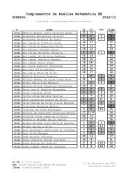
MIEBIOL 2012/13<br />
Complementos <strong>de</strong> Análise <strong>Matemática</strong> EE<br />
Folhas práticas<br />
Salvatore Cosentino<br />
<strong>Departamento</strong> <strong>de</strong> <strong>Matemática</strong> e Aplicações - Universi<strong>da</strong><strong>de</strong> <strong>do</strong> <strong>Minho</strong><br />
Campus <strong>de</strong> Gualtar, 4710 Braga - PORTUGAL<br />
gab B.4023, tel 253 604086<br />
e-mail scosentino@math.uminho.pt<br />
url http://w3.math.uminho.pt/~scosentino<br />
12 <strong>de</strong> Setembro <strong>de</strong> 2012<br />
This work is licensed un<strong>de</strong>r a<br />
Creative Commons Attribution-Noncommercial-ShareAlike 2.5 Portugal License.<br />
1
CONTEÚDO 2<br />
Conteú<strong>do</strong><br />
1 Equações diferenciais ordinárias 5<br />
2 Integração numérica e simulações* 9<br />
3 Teoremas <strong>de</strong> existência e unici<strong>da</strong><strong>de</strong>* 11<br />
4 EDOs simples e autónomas na reta 14<br />
5 Sistemas conservativos* 18<br />
6 EDOs lineares <strong>de</strong> primeira or<strong>de</strong>m 22<br />
7 EDOs separáveis e homogéneas 24<br />
8 EDOs exatas e campos conservativos 27<br />
9 EDOs lineares homogéneas com coeficientes constantes 30<br />
10 Números complexos e oscilações 33<br />
11 Variação <strong>do</strong>s parâmetros e coeficientes in<strong>de</strong>termina<strong>do</strong>s 36<br />
12 Oscila<strong>do</strong>r harmónico 38<br />
13 Simetrias e leis <strong>de</strong> conservação* 42<br />
14 Transforma<strong>da</strong> <strong>de</strong> Laplace 44<br />
15 Aplicações <strong>da</strong> transforma<strong>da</strong> <strong>de</strong> Laplace 48<br />
16 Sistemas lineares* 50<br />
17 Sistemas não lineares* 52<br />
18 Equações diferenciais parciais 59<br />
19 EDPs <strong>de</strong> primeira or<strong>de</strong>m* 61<br />
20 EDPs lineares <strong>de</strong> segun<strong>da</strong> or<strong>de</strong>m: Laplace, on<strong>da</strong>s e calor 63<br />
21 Separação <strong>de</strong> variáveis, harmónicas e mo<strong>do</strong>s 67<br />
22 Séries <strong>de</strong> Fourier 72<br />
23 Convergência <strong>da</strong>s séries <strong>de</strong> Fourier* 75<br />
24 Aplicações <strong>da</strong>s séries <strong>de</strong> Fourier às EDPs 78
CONTEÚDO 3<br />
Notações<br />
Números. N := {1, 2, 3, . . . } <strong>de</strong>nota o conjunto <strong>do</strong>s números naturais, N 0 := {0, 1, 2, 3, . . . }<br />
<strong>de</strong>nota o conjunto <strong>do</strong>s números inteiros não negativos. Z := {0, ±1, ±2, ±3, . . . } <strong>de</strong>nota o anel <strong>do</strong>s<br />
números inteiros. Q := {p/q com p, q, ∈ Z , q ≠ 0} <strong>de</strong>nota o corpo <strong>do</strong>s números racionais. R e C<br />
são os corpos <strong>do</strong>s númeors reais e complexos, respetivamente.<br />
Notação <strong>de</strong> Lan<strong>da</strong>u e . . . Sejam f(t) e g(t) duas funções <strong>de</strong>fini<strong>da</strong>s numa vizinhança <strong>do</strong> ponto<br />
a ∈ R ∪ { ± ∞}.<br />
f(t) = O(g(t)) (“f is big-O of g”) quan<strong>do</strong> t → a quer dizer que existe uma constante C > 0<br />
tal que f(t) ≤ C · g(t) para to<strong>do</strong>s os t numa vizinhança <strong>de</strong> a.<br />
f(t) = o(g(t)) (“f is small-o of g”) quan<strong>do</strong> t → a quer dizer que o quociente f(t)/g(t) → 0<br />
quan<strong>do</strong> t → a.<br />
f(t) ≍ g(t) (“f and g are within a boun<strong>de</strong>d ratio”) quan<strong>do</strong> t → a quer dizer que f(t) = O(g(t))<br />
e g(t) = O(f(t)), ou seja, que existe uma constante C > 0 tal que 1 C · g(t) ≤ f(t) ≤ C · g(t).<br />
f(x) ∼ g(x) (“f and g are asymptotically equal”) quan<strong>do</strong> t → a quer dizer que lim x→a f(x)/g(x) =<br />
1.<br />
Espaço euclidiano. R n <strong>de</strong>nota o espaço euclidiano <strong>de</strong> dimensão n. Fixa<strong>da</strong> a base canónica<br />
e 1 = (1, 0, . . . , 0), e 2 = (0, 1, 0, . . . ), . . . , e n = (0, . . . , 0, 1), os pontos <strong>de</strong> R n são os vetores<br />
x = (x 1 , x 2 , . . . , x n ) := x 1 e 1 + x 2 e 2 + · · · + x n e n<br />
<strong>de</strong> coor<strong>de</strong>na<strong>da</strong>s x i ∈ R, com i = 1, 2, . . . , n. Os pontos e as relativas coor<strong>de</strong>na<strong>da</strong>s no plano o<br />
ou no espaço 3-dimensional são também <strong>de</strong>nota<strong>do</strong>s, conforme a tradição, por r = (x, y) ∈ R 2 ou<br />
r = (x, y, z) ∈ R 3 .<br />
O produto interno euclidiano 〈·, ·〉 : R n × R n → R é <strong>de</strong>fini<strong>do</strong> por<br />
〈x, y〉 := x 1 y 1 + x 2 y 2 + · · · + x n y n .<br />
O produto interno realiza um isomorfismo entre o espaço dual (algébrico) (R n ) ′ := Hom R (R n , R)<br />
e o próprio R n : o valor <strong>da</strong> forma linear ξ ∈ (R n ) ′ ≃ R n no vetor x ∈ R n é ξ · x = 〈ξ, x〉.<br />
A norma euclidiana <strong>do</strong> vetor x ∈ R n é ‖x‖ := √ 〈x, x〉. A distância Euclidiana entre os pontos<br />
x, y ∈ R n é <strong>de</strong>fini<strong>da</strong> pelo teorema <strong>de</strong> Pitágoras<br />
d(x, y) := ‖x − y‖ = √ (x 1 − y 1 ) 2 + · · · + (x n − y n ) 2 .<br />
A bola aberta <strong>de</strong> centro a ∈ R n e raio r > 0 é o conjunto B r (a) := {x ∈ R n s.t. ‖x − a‖ < r}. Um<br />
subconjunto A ⊂ R n é aberto em R n se ca<strong>da</strong> seu ponto a ∈ A é o centro <strong>de</strong> uma bola B ε (a) ⊂ A,<br />
com ε > 0 suficientemente pequeno.<br />
Caminhos. Se t ↦→ x(t) = (x 1 (t), x 2 (t), . . . , x n (t)) ∈ R n é uma função diferenciável <strong>do</strong> “tempo”<br />
t ∈ I ⊂ R, ou seja, um caminho diferenciável <strong>de</strong>fini<strong>do</strong> num intervalo <strong>de</strong> tempos I ⊂ R com valores<br />
no espaço euclidiano R n , então as suas <strong>de</strong>riva<strong>da</strong>s são <strong>de</strong>nota<strong>da</strong>s por<br />
ẋ := dx<br />
dt ,<br />
ẍ := d2 x<br />
dt 2 , ...<br />
x := d3 x<br />
dt 3 , . . .<br />
Em particular, a primeira <strong>de</strong>riva<strong>da</strong> v(t) := ẋ(t) é dita “veloci<strong>da</strong><strong>de</strong>” <strong>da</strong> trajetória t ↦→ x(t no instante<br />
t), a sua norma v(t) := ‖v(t)‖ é dita “veloci<strong>da</strong><strong>de</strong> escalar”, e a segun<strong>da</strong> <strong>de</strong>riva<strong>da</strong> a(t) := ẍ(t) é dita<br />
“aceleração”.<br />
Campos. Um campo escalar é uma função real u : X ⊂ R n → R <strong>de</strong>fini<strong>da</strong> num <strong>do</strong>mínio X ⊂ R n .<br />
Um campo vetorial é uma função F : X ⊂ R n → R k , F(x) = (F 1 (x), F 2 (x), . . . , F k (x)), cujas<br />
coor<strong>de</strong>na<strong>da</strong>s F i (x) são k campos escalares.<br />
A <strong>de</strong>riva<strong>da</strong> <strong>do</strong> campo diferenciável F : X ⊂ R n → R k no ponto x ∈ X é a aplicação linear<br />
dF(x) : R n → R k tal que<br />
F(x + v) = F(x) + dF(x) · v + o(‖v‖)
CONTEÚDO 4<br />
para to<strong>do</strong>s os vetores v ∈ R n <strong>de</strong> norma ‖v‖ suficientemente pequena, <strong>de</strong>fini<strong>da</strong> em coor<strong>de</strong>na<strong>da</strong>s<br />
pela matriz Jacobiana JacF(x) := (∂F i /∂x j (x)) ∈ Mat k×n (R). Em particular, o diferencial <strong>do</strong><br />
campo escalar u : X ⊂ R n → R no ponto x ∈ X é a forma linear du(x) : R n → R,<br />
du(x) := ∂u<br />
∂x 1<br />
(x) dx 1 + ∂u<br />
∂x 2<br />
(x) dx 2 + · · · + ∂u<br />
∂x n<br />
(x) dx n<br />
(on<strong>de</strong> dx k , o diferencial <strong>da</strong> função coor<strong>de</strong>na<strong>da</strong> x ↦→ x k , é a forma linear que envia o vector v =<br />
(v 1 , v 2 , . . . , v n ) ∈ R n em dx k ·v := v k ). A <strong>de</strong>riva<strong>da</strong> <strong>do</strong> campo escalar diferenciável u : X ⊂ R n → R<br />
na direção <strong>do</strong> vetor v ∈ R n (aplica<strong>do</strong>) no ponto x ∈ X ⊂ R n , é igual, pela regra <strong>da</strong> ca<strong>de</strong>ia, a<br />
(£ v u)(x) := d dt u(x + tv) ∣<br />
∣∣∣t=0<br />
= du(x) · v .<br />
O gradiente <strong>do</strong> campo escalar diferenciável u : X ⊂ R n → é o campo vetorial ∇u : X ⊂ R n → R n<br />
tal que<br />
du(x) · v = 〈∇u(x), v〉<br />
para to<strong>do</strong> os vetores (tangentes) v ∈ R n (aplica<strong>do</strong>s no ponto x ∈ X).
1<br />
EQUAÇÕES DIFERENCIAIS ORDINÁRIAS 5<br />
1 Equações diferenciais ordinárias<br />
1. (partícula livre) A trajetória t ↦→ r(t) = (x(t), y(t), z(t)) ∈ R 3 <strong>de</strong> uma partícula livre <strong>de</strong><br />
massa m > 0 num referencial inercial é mo<strong>de</strong>la<strong>da</strong> pela equação <strong>de</strong> Newton<br />
d<br />
(mv) = 0 , ou seja, se m é constante, ma = 0 ,<br />
dt<br />
on<strong>de</strong> v(t) := ṙ(t) <strong>de</strong>nota a veloci<strong>da</strong><strong>de</strong> e a(t) := ¨r(t) <strong>de</strong>nota a aceleração <strong>da</strong> partícula. Em<br />
d<br />
particular, o momento linear p := mv é uma constante <strong>do</strong> movimento (ou seja,<br />
dtp = 0), <strong>de</strong><br />
acor<strong>do</strong> com o princípio <strong>de</strong> inércia <strong>de</strong> Galileo 1 ou a primeira lei <strong>de</strong> Newton 2 . As soluções <strong>da</strong><br />
equação <strong>de</strong> Newton <strong>da</strong> partícula livre são as retas afins<br />
r(t) = s + vt ,<br />
on<strong>de</strong> s = r(0) ∈ R 3 é a posição inicial s = r(0) e v = ṙ(0) ∈ R 3 é a veloci<strong>da</strong><strong>de</strong> (inicial).<br />
• Determine a trajetória <strong>de</strong> uma partícula livre que passa, no instante t 0 = 0, pela posição<br />
r(0) = (3, 2, 1) com veloci<strong>da</strong><strong>de</strong> ṙ(0) = (1, 2, 3).<br />
• Determine a trajetória <strong>de</strong> uma partícula livre que passa pela posição r(0) = (0, 1, 2)<br />
no instante t 0 = 0 e pela posição r(2) = (3, 4, 5) no instante t 1 = 2. Calcule a sua<br />
“veloci<strong>da</strong><strong>de</strong> escalar”, ou seja, a norma v := ‖v‖.<br />
2. (que<strong>da</strong> livre) A que<strong>da</strong> livre <strong>de</strong> uma partícula próxima <strong>da</strong> superfície terrestre é mo<strong>de</strong>la<strong>da</strong> pela<br />
equação <strong>de</strong> Newton<br />
m¨q = −mg<br />
on<strong>de</strong> q(t) ∈ R <strong>de</strong>nota a altura <strong>da</strong> partícula no instante t, m > 0 é a massa <strong>da</strong> partícula, e<br />
g ≃ 980 cm/s 2 é a aceleração <strong>da</strong> gravi<strong>da</strong><strong>de</strong> próximo <strong>da</strong> superfície terrestre. As soluções <strong>da</strong><br />
equação <strong>de</strong> Newton <strong>da</strong> que<strong>da</strong> livre são as parábolas<br />
q(t) = s + vt − 1 2 gt2 ,<br />
on<strong>de</strong> s = q(0) ∈ R é a altura inicial e v = ˙q(0) ∈ R é a veloci<strong>da</strong><strong>de</strong> inicial.<br />
• Uma pedra é <strong>de</strong>ixa<strong>da</strong> cair <strong>do</strong> topo <strong>da</strong> torre <strong>de</strong> Pisa, que tem cerca <strong>de</strong> 56 metros <strong>de</strong> altura,<br />
com veloci<strong>da</strong><strong>de</strong> inicial nula. Calcule a altura <strong>da</strong> pedra após 1 segun<strong>do</strong> e <strong>de</strong>termine o<br />
tempo necessário para a pedra atingir o chão.<br />
• Com que veloci<strong>da</strong><strong>de</strong> inicial <strong>de</strong>ve uma pedra ser atira<strong>da</strong> para cima <strong>de</strong> forma a atingir a<br />
altura <strong>de</strong> 20 metros, relativamente ao ponto inicial<br />
• Com que veloci<strong>da</strong><strong>de</strong> inicial <strong>de</strong>ve uma pedra ser atira<strong>da</strong> para cima <strong>de</strong> forma a voltar <strong>de</strong><br />
novo ao ponto <strong>de</strong> parti<strong>da</strong> ao fim <strong>de</strong> 10 segun<strong>do</strong>s<br />
3. (o exponencial) O exponencial (real) é a função exp : R → R, t ↦→ exp(t) = e t , <strong>de</strong>fini<strong>da</strong> pela<br />
série <strong>de</strong> potências<br />
e t := ∑ ∞<br />
n=0 tn<br />
n! = 1 + t + t2 2 + t3 6 + t4<br />
24 + . . . ,<br />
que converge uniformemente em ca<strong>da</strong> intervalo limita<strong>do</strong> <strong>da</strong> recta real. É imediato verificar<br />
que e 0 = 1, e que e t+s = e t e s para to<strong>do</strong>s os t, s ∈ R. Em particular, e t ≠ 0 para to<strong>do</strong>s os<br />
t ∈ R, e e −t = (e t ) −1 .<br />
• Verifique que x(t) = e t satisfaz a equação diferencial<br />
ẋ = x .<br />
Verifique que x(t) = x 0 e t é uma solução <strong>de</strong> ẋ = x com condição inicial x(0) = x 0 .<br />
1 “. . . il mobile durasse a muoversi tanto quanto durasse la lunghezza di quella superficie, né erta né china; se tale<br />
spazio fusse interminato, il moto in esso sarebbe parimenti senza termine, cioè perpetuo” [Galileo Galilei, Dialogo<br />
sopra i due massimi sistemi <strong>de</strong>l mon<strong>do</strong>, 1623.]<br />
2 “Lex prima: Corpus omne perseverare in statu suo quiescendi vel movendi uniformiter in directum, nisi quatenus<br />
a viribus impressis cogitur statum illum mutare” [Isaac Newton, Philosophiae Naturalis Principia Mathematica,<br />
1687.]
1<br />
EQUAÇÕES DIFERENCIAIS ORDINÁRIAS 6<br />
• Mostre que, se y(t) é uma solução <strong>de</strong> ẏ = y com condição inicial y(0) = x 0 , então o<br />
quociente y(t)/e t é constante e igual a x 0 (calcule a <strong>de</strong>riva<strong>da</strong> <strong>do</strong> quociente). Deduza<br />
que x 0 e t é a única solução <strong>de</strong> ẋ = x com condição inicial x(0) = x 0 .<br />
• Verifique que a função x(t) = e λt , com λ ∈ R, satisfaz a equação diferencial ẋ = λx.<br />
• Mostre que x(t) = x 0 e λt é a única solução <strong>da</strong> equação diferencial<br />
com condição inicial x(0) = x 0 .<br />
ẋ = λx<br />
4. (equações diferenciais ordinárias) Uma equação diferencial ordinária (EDO) <strong>de</strong> primeira or<strong>de</strong>m<br />
(resolúvel para a <strong>de</strong>riva<strong>da</strong>) é uma lei<br />
ẋ = v(t, x)<br />
para a trajetória t ↦→ x(t) <strong>de</strong> um sistema com espaço <strong>de</strong> fases X ⊂ R n , on<strong>de</strong> x(t) ∈ X <strong>de</strong>nota<br />
o esta<strong>do</strong> <strong>do</strong> sistema no instante t ∈ T ⊂ R, ẋ := dx<br />
dt<br />
<strong>de</strong>nota a <strong>de</strong>riva<strong>da</strong> <strong>do</strong> observável/is x em<br />
or<strong>de</strong>m ao tempo t, e v : T × X → R n é um campo <strong>de</strong> direções <strong>da</strong><strong>do</strong>.<br />
Uma solução <strong>de</strong> ẋ = v(t, x) é um caminho diferenciável t ↦→ x(t) cuja veloci<strong>da</strong><strong>de</strong> satisfaz<br />
ẋ(t) = v(t, x(t)) para ca<strong>da</strong> tempo t num intervalo I ⊂ T , ou seja, uma função x : I → X<br />
cujo gráfico Γ := {(t, x(t)) ∈ I × X com t ∈ I}, dito curva integral, é tangente ao campo<br />
<strong>de</strong> direções v(t, x) em ca<strong>da</strong> ponto (t, x(t)) ∈ Γ. Uma solução <strong>de</strong> ẋ = v(t, x) com condição<br />
inicial x(t 0 ) = x 0 ∈ X (ou solução <strong>do</strong> “problema <strong>de</strong> Cauchy”) é uma solução <strong>de</strong>fini<strong>da</strong> numa<br />
vizinhança <strong>de</strong> t 0 ∈ T , cujo gráfico contém o ponto (t 0 , x 0 ) ∈ T × X.<br />
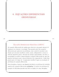
Campo <strong>de</strong> direções e uma solução <strong>de</strong> ẋ = sin(x)(1 − t 2 ).<br />
O teorema <strong>de</strong> Peano 3 4 afirma que, se o campo v(t, x) é contínuo, então existem sempre<br />
soluções locais (i.e. <strong>de</strong>fini<strong>da</strong>s em vizinhanças suficientemente pequenas <strong>do</strong> tempo inicial)<br />
<strong>do</strong> problema <strong>de</strong> Cauchy. O teorema <strong>de</strong> Picard-Lin<strong>de</strong>löf 5 afirma que, se o campo v(t, x) é<br />
contínuo e localmente Lipschitziano 6 (por exemplo, diferenciável <strong>de</strong> classe C 1 ) na variável<br />
x, então para ca<strong>da</strong> ponto (t 0 , x 0 ) ∈ T × X passa uma única solução com condição inicial<br />
x(t 0 ) = x 0 .<br />
• Esboce o campo <strong>de</strong> direções <strong>da</strong>s EDOs<br />
ẋ = t ẋ = −x + t ẋ = sin(t)<br />
e conjeture sobre o comportamento qualitativo <strong>da</strong>s soluções.<br />
3 G. Peano, Sull’integrabilità <strong>de</strong>lle equazioni differenziali <strong>de</strong>l primo ordine, Atti Accad. Sci. Torino 21 (1886),<br />
677-685.<br />
4 G. Peano, Demonstration <strong>de</strong> l’intégrabilité <strong>de</strong>s équations différentielles ordinaires, Mathematische Annalen 37<br />
(1890) 182-228.<br />
5 M. E. Lin<strong>de</strong>löf, Sur l’application <strong>de</strong> la métho<strong>de</strong> <strong>de</strong>s approximations successives aux équations différentielles<br />
ordinaires du premier ordre, Comptes rendus heb<strong>do</strong>ma<strong>da</strong>ires <strong>de</strong>s séances <strong>de</strong> l’Académie <strong>de</strong>s sciences 114 (1894),<br />
454-457.<br />
6 A função f : U → R m é Lipschitziana no <strong>do</strong>mínio U ⊂ R n se<br />
∃ L > 0 t.q. ‖f(x) − f(y)‖ ≤ L · ‖x − y‖ ∀ x, y ∈ U .
1<br />
EQUAÇÕES DIFERENCIAIS ORDINÁRIAS 7<br />
• A função x(t) = t 3 é solução <strong>da</strong> equação diferencial ẋ = 3x 2/3 com condição inicial<br />
x(0) = 0 E a função x(t) = 0 <br />
• Determine uma equação diferencial <strong>de</strong> primeira or<strong>de</strong>m e uma equação diferencial <strong>de</strong><br />
segun<strong>da</strong> or<strong>de</strong>m que admitam como solução a Gaussiana ϕ(t) = e −t2 /2 .<br />
5. (soluções <strong>de</strong> Chandrasekhar <strong>da</strong> equação <strong>de</strong> Lane-Em<strong>de</strong>n) Um mo<strong>de</strong>lo <strong>do</strong> perfil <strong>de</strong> equilíbrio<br />
hidrostático <strong>de</strong> uma estrela é a equação <strong>de</strong> Lane-Em<strong>de</strong>n<br />
(<br />
1 d<br />
ξ 2 ξ 2 dθ )<br />
= −θ p ,<br />
dξ dξ<br />
on<strong>de</strong> ξ ≥ 0 é uma “distância adimensional” <strong>do</strong> centro <strong>da</strong> estrela, θ(ξ) é proporcional à<br />
<strong>de</strong>nsi<strong>da</strong><strong>de</strong>, e p é um parâmetro que <strong>de</strong>pen<strong>de</strong> <strong>da</strong> equação <strong>de</strong> esta<strong>do</strong> P = Kρ 1+1/p <strong>do</strong> gás que<br />
forma a estrela. O problema físico é <strong>de</strong>terminare a solução com condições iniciais θ(0) = 1 e<br />
dθ/dξ(0) = 0, e o menor zero <strong>de</strong> θ(ξ) com ξ > 0 é interpreta<strong>do</strong> como sen<strong>do</strong> o raio <strong>da</strong> estrela.<br />
• Verifique que 7<br />
θ(ξ) = 1 − 1 6 ξ2 ,<br />
θ(ξ) = sin ξ<br />
ξ<br />
1<br />
e θ(ξ) = √<br />
1 + 1 3 ξ2<br />
são soluções <strong>da</strong> equação <strong>de</strong> Lane-Em<strong>de</strong>n quan<strong>do</strong> p = 0, 1 e 5, respetivamente.<br />
6. (campos <strong>de</strong> vetores e EDOs autónomas) Um campo <strong>de</strong> vetores v : X → R n no espaço <strong>de</strong> fases<br />
X ⊂ R n <strong>de</strong>fine uma equação diferencial ordinária autónoma (que não <strong>de</strong>pen<strong>de</strong> explicitamente<br />
<strong>do</strong> tempo, como to<strong>da</strong>s as leis fun<strong>da</strong>mentais <strong>da</strong> física)<br />
ẋ = v(x) .<br />
As imagens x(I) = {x(t) com t ∈ I} ⊂ X <strong>da</strong>s soluções/trajetórias x : I → X no espaço<br />
<strong>de</strong> fases são ditas órbitas, ou curvas <strong>de</strong> fases, <strong>do</strong> sistema autónomo. Se x ∈ X é um ponto<br />
singular <strong>do</strong> campo, i.e. um ponto on<strong>de</strong> v(x) = 0, então o caminho constante x(t) = x ∀t ∈ R<br />
é uma solução, dita solução <strong>de</strong> equilíbrio, ou estacionária.<br />
Campo <strong>de</strong> vetores e uma curva <strong>de</strong> fases <strong>do</strong> pêndulo com atrito,<br />
˙q = p, ṗ = − sin(q) − p/2.<br />
• Esboce o campo <strong>de</strong> direções e o campo <strong>de</strong> vetores <strong>da</strong>s EDOs autónomas<br />
ẋ = −x ẋ = x − 1 ẋ = x(1 − x)<br />
ẋ = (x − 1)(x − 2)(x − 3) ẋ = (x − 1) 2 (x − 2) 2<br />
{ { { ˙q = p<br />
˙q = 2q<br />
˙q = q − p<br />
ṗ = −q ṗ = −p/2 ṗ = p − q<br />
<strong>de</strong>termine as soluções <strong>de</strong> equilíbrio, e conjeture sobre o comportamento qualitativo <strong>da</strong>s<br />
(outras) soluções.<br />
7 Subrahmanyan Chandrasekhar, An Introduction to the Study of Stellar Structure, Dover, 1958.
1<br />
EQUAÇÕES DIFERENCIAIS ORDINÁRIAS 8<br />
7. (campos completos e fluxos <strong>de</strong> fases) Seja v : X ⊂ R n → R n um campo <strong>de</strong> vetores <strong>de</strong>fini<strong>do</strong><br />
num <strong>do</strong>mínio X ⊂ R n (ou numa varie<strong>da</strong><strong>de</strong> diferenciável). Se por ca<strong>da</strong> ponto x 0 ∈ X<br />
<strong>do</strong> espaço <strong>de</strong> fases passa uma e uma única solução global (ou seja, <strong>de</strong>fini<strong>da</strong> para to<strong>do</strong>s os<br />
tempos) ϕ : R → X, t ↦→ ϕ(t), com condição inicial ϕ(0) = x 0 , então o campo <strong>de</strong> vetores é dito<br />
completo. Um campo completo <strong>de</strong>fine/gera um fluxo <strong>de</strong> fases, um grupo <strong>de</strong> transformações<br />
Φ t = e tv : X → X, com t ∈ R, tais que<br />
Φ t ◦ Φ s = Φ t+s e Φ 0 = id X ∀ t, s, ∈ R .<br />
O ponto Φ t (x 0 ) é o esta<strong>do</strong> no tempo t <strong>da</strong> solução que passa por x 0 no instante 0. Vice-versa,<br />
um fluxo <strong>de</strong> fases diferenciável <strong>de</strong>fine um campo <strong>de</strong> vetores<br />
Φ t (x) − x<br />
v(x) := lim ,<br />
t→0 t<br />
dito “gera<strong>do</strong>r infinitesimal” <strong>do</strong> grupo <strong>de</strong> transformações. As curvas t ↦→ Φ t (x 0 ) são as soluções<br />
<strong>de</strong> ẋ = v(x) com condição inicial x(0) = x 0 .<br />
• Determine os campos <strong>de</strong> vetores que geram os seguintes fluxos no plano R 2<br />
Φ t (x, y) = (e λt x , e µt y)<br />
Φ t (x, y) = (cos(t) x − sin(t) y , sin(t) x + cos(t) y)<br />
Φ t (x, y) = (x + ty , y)<br />
8. (quase to<strong>da</strong>s as EDOs têm or<strong>de</strong>m um!) A EDO <strong>de</strong> or<strong>de</strong>m n ≥ 2 (resolúvel para a n-ésima<br />
<strong>de</strong>riva<strong>da</strong>)<br />
y (n) = F<br />
(t, y, ẏ, ÿ, ..., y (n−1))<br />
para o observável y(t) ∈ R é equivalente à EDO (ou sistema <strong>de</strong> EDOs) <strong>de</strong> primeira or<strong>de</strong>m<br />
ẋ = v (t, x)<br />
para o observável x = (x 1 , x 2 , ..., x n ) ∈ R n <strong>de</strong>fini<strong>do</strong> por<br />
x 1 := y x 2 := ẏ x 3 := ÿ ... x n := y (n−1) ,<br />
on<strong>de</strong> o campo <strong>de</strong> direções é v(t, x) := (x 2 , ..., x n−1 , F (t, x 1 , x 2 , ..., x n )).<br />
• Determine os sistemas <strong>de</strong> ODEs <strong>de</strong> or<strong>de</strong>m 1 que traduzem as seguintes ODEs <strong>de</strong> or<strong>de</strong>m<br />
> 1<br />
ẍ = −x ẍ + ẋ = 0 ẍ + ẋ + x = 0<br />
...<br />
ẍ = t − x ẍ + ẋ + x = 0 x = x
2<br />
INTEGRAÇÃO NUMÉRICA E SIMULAÇÕES* 9<br />
2 Integração numérica e simulações*<br />
1. (méto<strong>do</strong> <strong>de</strong> Euler) Consi<strong>de</strong>re o problema <strong>de</strong> simular as soluções <strong>da</strong> EDO ẋ = v(t, x). O<br />
méto<strong>do</strong> <strong>de</strong> Euler consiste em utilizar recursivamente a aproximação linear<br />
x(t + dt) ≃ x(t) + v(t, x) · dt ,<br />
<strong>da</strong><strong>do</strong> um “passo” dt suficientemente pequeno. Portanto, a solução x(t n ), nos tempos t n =<br />
t 0 + n · dt, com condição inicial x(t 0 ) = x 0 é estima<strong>da</strong> pela sucessão (x n ) n∈N0 <strong>de</strong>fini<strong>da</strong><br />
recursivamente por<br />
x n+1 = x n + v(t n , x n ) · dt .<br />
Numa linguagem como c++ ou Java, o ciclo para obter uma aproximação <strong>de</strong> x(t), <strong>da</strong><strong>do</strong><br />
x(t 0 ) = x, é<br />
while (time < t)<br />
{<br />
x += v(time, x) * dt ;<br />
time += dt ;<br />
}<br />
• Consi<strong>de</strong>re a equação diferencial<br />
ẋ = x<br />
com condição inicial x(0) = 1. Mostre que, se o passo é dt = ε e o tempo final é t = nε<br />
com n ∈ N, então o méto<strong>do</strong> <strong>de</strong> Euler fornece a aproximação<br />
x(t) ≃ x n = (1 + ε) n<br />
on<strong>de</strong> n = t/ε é o número <strong>de</strong> passos. Deduza que, no limite quan<strong>do</strong> o passo ε → 0, as<br />
aproximações convergem para a solução e t , pois<br />
(<br />
lim (1 +<br />
ε→0 ε)t/ε = lim 1 + t ) n<br />
n→∞ n<br />
• Simule a solução <strong>da</strong> EDO ẋ = (1 − 2t) x com condição inicial x(0) = 1. Compare o<br />
resulta<strong>do</strong> com o valor exacto x(t) = e t−t2 , usan<strong>do</strong> passos diferentes, por exemplo 0.01,<br />
0.001, 0.0001 ...<br />
• Aproxime, usan<strong>do</strong> o méto<strong>do</strong> <strong>de</strong> Euler, a solução <strong>do</strong> oscila<strong>do</strong>r harmónico<br />
{ ˙q = p<br />
ṗ = −q<br />
com condição inicial q(0) = 1 e p(0) = 0. Compare o valor <strong>de</strong> q(1) com o valor exacto<br />
q(1) = cos(1), usan<strong>do</strong> passos diferentes, por exemplo 0.1, 0.01, 0.001, 0.0001 ...<br />
2. (méto<strong>do</strong> RK-4) O méto<strong>do</strong> <strong>de</strong> Runge-Kutta (<strong>de</strong> or<strong>de</strong>m) 4 para simular a solução <strong>de</strong><br />
ẋ = v(t, x) com condição inicial x(t 0 ) = x 0<br />
consiste em escolher um “passo” dt, e aproximar x(t 0 + n · dt) com a sucessão (x n ) <strong>de</strong>fini<strong>da</strong><br />
recursivamente por<br />
x n+1 = x n + dt<br />
6 (k 1 + 2k 2 + 2k 3 + k 4 )<br />
on<strong>de</strong> t n = t 0 + n · dt, e os coeficientes k 1 , k 2 , k 3 e k 4 são <strong>de</strong>fini<strong>do</strong>s recursivamente por<br />
k 1 = v(t n , x n )<br />
k 2 = v ( t n + dt<br />
2 , x n + dt<br />
2 · k )<br />
1<br />
k 3 = v ( t n + dt<br />
2 , x n + dt<br />
2 · k )<br />
2<br />
• Implemente um código para simular sistemas <strong>de</strong> EDOs usan<strong>do</strong> o méto<strong>do</strong> RK-4.<br />
k 4 = v(t n + dt, x n + dt · k 3 )
2<br />
INTEGRAÇÃO NUMÉRICA E SIMULAÇÕES* 10<br />
3. (simulações com software proprietário) Existem software proprietários que permitem resolver<br />
analiticamente, quan<strong>do</strong> possível, ou fazer simulações numéricas <strong>de</strong> equações diferenciais<br />
ordinarias e parciais. Por exemplo, a função o<strong>de</strong>45 <strong>do</strong> MATLAB R○ , ou a função NDSolve <strong>do</strong><br />
Mathematica R○ , calculam soluções aproxima<strong>da</strong>s <strong>de</strong> EDOs ẋ = v(t, x) utilizan<strong>do</strong> variações <strong>do</strong><br />
méto<strong>do</strong> <strong>de</strong> Runge-Kutta.<br />
• Verifique se os PC <strong>do</strong> seu <strong>Departamento</strong>/<strong>da</strong> sua Universi<strong>da</strong><strong>de</strong> têm accesso a um <strong>do</strong>s<br />
software proprietários MATLAB R○ ou Mathematica R○ .<br />
• Em caso afirmativo, apren<strong>da</strong> a usar as funções o<strong>de</strong>45 ou NDSolve.<br />
Por exemplo, o pêndulo com atrito po<strong>de</strong> ser simula<strong>do</strong>, no Mathematica R○ , usan<strong>do</strong> as<br />
instruções<br />
s = NDSolve[{x’[t] == y[t], y’[t] == -Sin[x[t]] - 0.7 y[t],<br />
x[0] == y[0] == 1}, {x, y}, {t, 20}]<br />
ParametricPlot[Evaluate[{x[t], y[t]} /. s], {t, 0, 20}]<br />
O resulta<strong>do</strong> é<br />
0.2<br />
0.1<br />
0.3 0.2 0.1 0.1 0.2 0.3<br />
0.1<br />
0.2
3 TEOREMAS DE EXISTÊNCIA E UNICIDADE* 11<br />
3 Teoremas <strong>de</strong> existência e unici<strong>da</strong><strong>de</strong>*<br />
1. (iterações <strong>de</strong> Picard) Uma função diferenciável t ↦→ ϕ(t), <strong>de</strong>fini<strong>da</strong> num intervalo I ⊂ R e com<br />
valores num <strong>do</strong>mínio X ⊂ R n , é solução <strong>da</strong> equação diferencial ẋ = v(t, x) com condição<br />
inicial ϕ(t 0 ) = x 0 se e só se<br />
∫ t<br />
ϕ(t) = x 0 + v (s, ϕ(s)) ds ,<br />
t 0<br />
ou seja, se ϕ(t) é um ponto fixo <strong>do</strong> mapa <strong>de</strong> Picard P : C(I, X) → C(I, X), que envia uma<br />
função φ(t) na função<br />
(Pφ) (t) := x 0 + ∫ t<br />
t 0<br />
v (s, φ(s)) ds .<br />
Se a sucessão <strong>de</strong> funções φ, Pφ, P 2 φ := P (Pφ) , . . . , P n φ := P ( P n−1 φ ) , . . . , obti<strong>da</strong>s<br />
iteran<strong>do</strong> o mapa <strong>de</strong> Picard a partir <strong>de</strong> uma função inicial φ, é convergente (numa topologia<br />
apropria<strong>da</strong> <strong>de</strong>fini<strong>da</strong> num subespaço C ⊂ C(I, X) := {φ : I → X contínua} tal que P : C → C<br />
seja contínua), então o limite x(t) = lim n→∞ (P n φ) (t) é um ponto fixo <strong>do</strong> mapa <strong>de</strong> Picard,<br />
e portanto uma solução <strong>da</strong> equação diferencial ẋ = v(t, x) com a condição inicial <strong>da</strong><strong>da</strong><br />
x(t 0 ) = x 0 .<br />
• Se o campo <strong>de</strong> veloci<strong>da</strong><strong>de</strong>s apenas <strong>de</strong>pen<strong>de</strong> <strong>do</strong> tempo, então o mapa <strong>de</strong> Picard envia<br />
to<strong>da</strong> função inicial φ(t) na solução<br />
<strong>da</strong> EDO simples ẋ = v(t) com x(t 0 ) = x 0 .<br />
∫ t<br />
(Pφ) (t) = x 0 + v (s) ds<br />
t 0<br />
• Suppose you want to solve ẋ = x with initial condition x(0) = 1. You start with the<br />
guess φ(t) = 1, and then compute<br />
(Pφ) (t) = 1+t<br />
(<br />
P 2 φ ) (t) = 1+t+ 1 2 t2 . . . (P n φ) (t) = 1+t+ 1 2 t2 +· · ·+ 1 n! tn<br />
Hence the sequence converges (uniformly on boun<strong>de</strong>d intervals) to the Taylor series of<br />
the exponential function<br />
which is the solution we already knew.<br />
(P n φ) (t) → 1 + t + 1 2 t2 + · · · + 1 n! tn + ... = e t ,<br />
2. (contrações e teorema <strong>de</strong> ponto fixo <strong>de</strong> Banach) Seja (X, d) um espaço métrico. Uma transformação<br />
f : X → X é uma contração (ou λ-contração se é importante lembrar o valor <strong>de</strong><br />
λ) se é Lipschitz e tem constante <strong>de</strong> Lipschitz λ < 1, ou seja, se existe 0 ≤ λ < 1 tal que<br />
para to<strong>do</strong>s x, x ′ ∈ X<br />
d(f(x), f(x ′ )) ≤ λ · d(x, x ′ ) .<br />
As trajetórias <strong>da</strong> transformação f : X → X são as sucessões (x n ) <strong>de</strong>fini<strong>da</strong>s recursivamente<br />
por x n+1 = f(x n ), se n ≥ 0, a partir <strong>de</strong> uma condição inicial x 0 ∈ X. Os pontos fixos <strong>de</strong> f<br />
são os pontos p ∈ X tas que f(p) = p.<br />
O princípio <strong>da</strong>s contrações (a.k.a. teorema <strong>de</strong> ponto fixo <strong>de</strong> Banach) afirma que “to<strong>da</strong>s as trajetórias<br />
<strong>de</strong> uma contração f : X → X são sucesssões <strong>de</strong> Cauchy, e a distância entre ca<strong>da</strong> duas<br />
trajetórias diminue exponencialmente no tempo. Em particular, se X é completo, então f<br />
admite um único ponto fixo p, e a trajetória <strong>de</strong> to<strong>do</strong> ponto x ∈ X converge exponencialmente<br />
para o ponto fixo, i.e. f n (x) → p quan<strong>do</strong> n → ∞”.<br />
Demonstração. Seja f : X → X uma λ-contração. Seja x 0 ∈ X um ponto arbitrário, e seja<br />
(x n) a sua trajetória, ou seja, a sucessão <strong>de</strong>fini<strong>da</strong> recursivamente por x n+1 = f(x n). Usan<strong>do</strong>
3 TEOREMAS DE EXISTÊNCIA E UNICIDADE* 12<br />
k-vezes a contrativi<strong>da</strong><strong>de</strong> ve-se que d (x k+1 , x k ) ≤ d(x 1 , x 0 ) · λ k , e portanto que<br />
d(x n+k , x n)<br />
≤<br />
k−1 X<br />
k−1 X<br />
d(x n+j+1 , x n+j ) ≤ d(x 1 , x 0 ) · λ n+j<br />
j=0<br />
≤ d(x 1 , x 0 ) · λ n ·<br />
j=0<br />
∞X<br />
λ j ≤<br />
λn<br />
1 − λ · d(x 1, x 0 ) .<br />
j=0<br />
Em particular, (x n) é uma sucessão <strong>de</strong> Cauchy. O limite p = lim n→∞ x n, que existe se X<br />
é completo, é um ponto fixo <strong>de</strong> f, porque f é contínua. Se p e p ′ são pontos fixos, então<br />
d(p, p ′ ) = d(f(p), f(p ′ )) ≤ λd(p, p ′ ) com λ < 1 implica que d(p, p ′ ) = 0, o que mostra que o ponto<br />
fixo é único. Usan<strong>do</strong> a contrativi<strong>da</strong><strong>de</strong> também ve-se que d(x n, p) ≤ λ n · d(x 0 , p), ou seja que a<br />
convergência x n → p é exponencial.<br />
• Utilize o teorema <strong>do</strong> valor médio para mostrar que uma função f : R n → R n <strong>de</strong> classe<br />
C 1 é uma contração sse existe λ < 1 tal que |f ′ (x)| ≤ λ para to<strong>do</strong> x ∈ R n .<br />
• Mostre que uma transformação f : X → X tal que<br />
d(f(x), f(x ′ )) < d(x, x ′ )<br />
para to<strong>do</strong>s x, x ′ ∈ X distintos po<strong>de</strong> não ter pontos fixos, mesmo se o espaço métrico X<br />
for completo.<br />
3. (teorema <strong>de</strong> Picard-Lin<strong>de</strong>löf 8 .) Seja v(t, x) um campo <strong>de</strong> veloci<strong>da</strong><strong>de</strong>s contínuo <strong>de</strong>fini<strong>do</strong> num<br />
<strong>do</strong>mínio D <strong>do</strong> espaço <strong>de</strong> fases extendi<strong>do</strong> R×X. Se v é localmente Lipschitziana (por exemplo,<br />
diferenciável com continui<strong>da</strong><strong>de</strong>) com respeito a segun<strong>da</strong> variável x ∈ X ⊂ R n , então existe<br />
uma e uma única solução local <strong>da</strong> equação diferencial ẋ = v(t, x) que passa por ca<strong>da</strong> ponto<br />
(t 0 , x 0 ) ∈ D.<br />
Proof. In<strong>de</strong>ed, choose a sufficiently small rectangular neighborhood I × B = [t 0 − ε, t 0 + ε] ×<br />
B δ (x 0 ) around (t 0 , x 0 ), where B = B δ (x 0 ) <strong>de</strong>notes the closed ball with center x 0 and radius<br />
δ in X. There follows from continuity of v that there exists K such that |v(t, x)| ≤ K for any<br />
(t, x) ∈ I × B. There follows from the local Lipschitz condition for v that there exists M such<br />
that |v(t, x) − v(t, y)| ≤ M|x − y| for any t ∈ I and any x, y ∈ B. Now restrict, if nee<strong>de</strong>d, the<br />
(radius of the) interval I in such a way to get both the inequalities Kε ≤ δ and Mε < 1. Let<br />
C = C 0 (I, B) be the space of continuous functions t ↦→ φ(t) sending I into B. Equipped with<br />
the sup norm ‖φ − ϕ‖ ∞ := sup t∈I |φ(t) − ϕ(t)| this is a complete space. One verifies that the<br />
Picard’s map sends C into C, since<br />
Z t<br />
| (Pφ) (t) − x 0 | ≤ |v (s, φ(s)) | ds ≤ Kε ≤ δ .<br />
t 0<br />
Finally, given two functions φ, ϕ ∈ C, one sees that<br />
Z t<br />
| (Pφ) (t) − (Pϕ) (t)| ≤ |v (s, φ(s)) − v (s, ϕ(s)) | ds ≤ Mε · sup |φ(t) − ϕ(t)| ,<br />
t 0 t∈I<br />
hence ‖Pφ − Pϕ‖ ∞ < Mε · ‖φ − ϕ‖ ∞. Since λ := Mε < 1, this proves that the Picard’s map is<br />
a contraction and the Banach fixed point theorem allows to conclu<strong>de</strong>.<br />
4. (lema <strong>de</strong> Gromwall 9 ) Let φ(t) and ψ(t) be two non-negative real valued functions <strong>de</strong>fined in<br />
the interval [a, b], and assume that<br />
φ(t) ≤ K +<br />
∫ t<br />
for any a ≤ t ≤ b and some constant K ≥ 0. Then<br />
a<br />
ψ(s)φ(s) ds<br />
φ(t) ≤ Ke R t<br />
a ψ(s) ds .<br />
8 M. E. Lin<strong>de</strong>löf, Sur l’application <strong>de</strong> la métho<strong>de</strong> <strong>de</strong>s approximations successives aux équations différentielles<br />
ordinaires du premier ordre, Comptes rendus heb<strong>do</strong>ma<strong>da</strong>ires <strong>de</strong>s séances <strong>de</strong> l’Académie <strong>de</strong>s sciences 114 (1894),<br />
454-457.<br />
9 T.H. Gronwall, Note on the <strong>de</strong>rivative with respect to a parameter of the solutions of a system of differential<br />
equations, Ann. of Math 20 (1919), 292-296.
3 TEOREMAS DE EXISTÊNCIA E UNICIDADE* 13<br />
Proof. In<strong>de</strong>ed, assume that K > 0. Define Φ(t) := K + R t<br />
a ψ(s)φ(s) ds and observe that<br />
Φ(a) = K > 0, hence Φ(t) > 0 for all a ≤ t ≤ b. The logarithmic <strong>de</strong>rivative is<br />
d<br />
ψ(t)φ(t)<br />
log Φ(t) = ≤ ψ(t)<br />
dt Φ(t)<br />
where we used the hypothesis φ(t) ≤ Φ(t). Integrating the inequality we get, for a ≤ t ≤ b,<br />
Z t<br />
log Φ(t) ≤ Φ(a) + ψ(s) ds .<br />
a<br />
Exponentiation gives the result, since<br />
φ(t) ≤ Φ(t) ≤ K · eR ta<br />
ψ(s) ds .<br />
The case K = 0 follows taking the limit of the above inequalities along a sequence of K n > 0<br />
<strong>de</strong>creasing to zero.<br />
5. (<strong>de</strong>pen<strong>de</strong>nce on initial <strong>da</strong>ta and parameters)
4 EDOS SIMPLES E AUTÓNOMAS NA RETA 14<br />
4 EDOs simples e autónomas na reta<br />
1. (integração <strong>de</strong> EDOs simples) O teorema (fun<strong>da</strong>mental <strong>do</strong> cálculo) <strong>de</strong> Newton e Leibniz 10<br />
afirma que a <strong>de</strong>riva<strong>da</strong> <strong>do</strong> integral in<strong>de</strong>fini<strong>do</strong> F (t) := ∫ t<br />
f(s) ds <strong>de</strong> uma função contínua f(t)<br />
a<br />
existe e é igual a F ′ (t) = f(t). Portanto, se v(t) é um campo <strong>de</strong> direções contínuo, a solução<br />
<strong>da</strong> EDO<br />
ẋ = v(t)<br />
com condição inicial x(t 0 ) = x 0 é <strong>de</strong>termina<strong>da</strong> por meio <strong>de</strong> uma integração, ou seja,<br />
ẋ = v(t) , x(t 0 ) = x 0 ⇒ x(t) = x 0 + ∫ t<br />
t 0<br />
v(s)ds<br />
(<strong>do</strong>n<strong>de</strong> a tradição <strong>de</strong> dizer “integrar” uma equação diferencial em vez <strong>de</strong> “resolver”). Se x(t)<br />
é solução <strong>de</strong> ẋ = v(t), então também x(t) + c é solução, ∀c ∈ R.<br />
• Integre as seguintes EDOs, <strong>de</strong>fini<strong>da</strong>s em oportunos intervalos <strong>de</strong> tempo<br />
ẋ = 2 − t + 3t 2 + 5t 6 ẋ = e −t ẋ = cos(3t) ẋ = 1/t<br />
2. (foguetão) Se um foguetão <strong>de</strong> massa m(t) no espaço vazio (ou seja, sem forças gravitacionais!)<br />
expulsa combustível a uma veloci<strong>da</strong><strong>de</strong> relativa constante −V e a uma taxa constante ṁ = −α,<br />
então a sua trajetória num referencial inercial é mo<strong>de</strong>la<strong>da</strong> pela equação <strong>de</strong> Newton<br />
d<br />
(mv) = α(V − v) , ou seja , ṁv + m ˙v = α(V − v) .<br />
dt<br />
• Resolva a EDO ṁ = −α para a massa <strong>do</strong> foguetão, com massa inicial m(0) = m 0 > 0,<br />
e substitua o resulta<strong>do</strong> na equação <strong>de</strong> Newton, obten<strong>do</strong><br />
(<strong>de</strong>s<strong>de</strong> que 0 ≤ t < m 0 /α).<br />
˙v =<br />
αV<br />
m 0 − αt<br />
• Calcule a trajetória <strong>do</strong> foguetão com veloci<strong>da</strong><strong>de</strong> inicial v(0) = v 0 e posição inicial q(0) =<br />
0, váli<strong>da</strong> para tempos t inferiores ao tempo necessário para acabar o combustível.<br />
3. (campos <strong>de</strong> vetores e EDOs autónomas na reta) Um campo <strong>de</strong> vetores v : X → R, <strong>de</strong>fini<strong>do</strong><br />
num intervalo X ⊂ R, <strong>de</strong>fine uma EDO autónoma<br />
ẋ = v(x) .<br />
Se x 0 é um ponto singular <strong>de</strong> v(x), i.e. um ponto on<strong>de</strong> v(x 0 ) = 0, então x(t) = x 0 ∀t ∈ R<br />
é uma solução estacionária (ou <strong>de</strong> equilíbrio) <strong>da</strong> equação. Se x 0 é um ponto não singular<br />
<strong>do</strong> campo contínuo v(x), i.e. se v(x 0 ) ≠ 0, então uma solução local com condição inicial<br />
x(t 0 ) = x 0 po<strong>de</strong> ser <strong>de</strong>terminan<strong>da</strong> “separan<strong>do</strong> as variáveis”, ou seja, fazen<strong>do</strong><br />
integran<strong>do</strong> os <strong>do</strong>is membros, ∫ dx<br />
v(x) = ∫ dt. Ou seja,<br />
ẋ = v(x) , x(t 0 ) = x 0<br />
Se o campo v(x) é diferenciável, estas soluções são únicas.<br />
10 A solução <strong>do</strong> anagrama<br />
6acc<strong>da</strong>e13eff7i3l9n4o4qrr4s8t12vx<br />
⇒<br />
{<br />
∫ x<br />
x 0<br />
x(t) = x 0 se v(x 0 ) = 0<br />
dy<br />
v(y) = t − t 0 se v(x 0 ) ≠ 0<br />
dx<br />
v(x)<br />
= dt e<br />
conti<strong>do</strong> numa carta <strong>de</strong> Isaac Newton dirigi<strong>da</strong> a Gottfried Leibniz em 1677, é “Data aequatione quotcunque fluentes<br />
quantitates involvente fluxiones invenire et vice versa”.
4 EDOS SIMPLES E AUTÓNOMAS NA RETA 15<br />
Proof. In<strong>de</strong>ed, assume that the velocity field v is continuous and let J = (x − , x + ) be the<br />
maximal interval containing x 0 where v is different from zero. Define a function H : R × J → R<br />
as<br />
Z x dy<br />
H(t, x) = t − t 0 −<br />
x 0<br />
v(y) .<br />
If t ↦→ ϕ(t) is a solution of the Cauchy problem, then computation shows that d H (t, ϕ(t)) = 0<br />
dt<br />
for any time t. There follows that H is constant along the solutions of the Cauchy problem.<br />
Since H(t 0 , x 0 ) = 0, we conclu<strong>de</strong> that the graph of any solution belongs to the level set Σ =<br />
{(t, x) ∈ R × J s.t. H(t, x) = 0}. Now observe that H is continuously differentiable and that its<br />
differential dH = dt + dx/v(x) is never zero. Actually, both partial <strong>de</strong>rivatives ∂H/∂t and ∂H/∂x<br />
are always different from zero. Hence we can apply the implicit function theorem and conclu<strong>de</strong><br />
that the level set Σ is, in some neighborhood I × J of (t 0 , x 0 ), the graph of a unique differentiable<br />
function x ↦→ t(x), as well as the graph of a unique differentiable function t ↦→ x(t), the inverse<br />
of t, which solves the<br />
“<br />
Cauchy<br />
”<br />
problem: just compute the <strong>de</strong>rivative (using the inverse function<br />
theorem), ẋ(t) = 1/ dt<br />
dx (x(t)) = v(x), and check the initial condition. Observe that the function<br />
t(x) − t 0 has then the interpretation of the “time nee<strong>de</strong>d to go from x 0 to x”.<br />
Se x(t) é solução <strong>de</strong> ẋ = v(x), então também x(t − c) é solução, ∀c ∈ R (a física mo<strong>de</strong>la<strong>da</strong><br />
por uma EDO autónoma é invariante para translações no tempo).<br />
• Consi<strong>de</strong>re as seguintes EDOs autónomas<br />
ẋ = −3x ẋ = x − 1 ẋ = x 2 ẋ = √ x<br />
ẋ = (x − 1)(x − 2) ẋ = e x ẋ = (x − 1)(x − 2)(x − 3)<br />
<strong>de</strong>fini<strong>da</strong>s em intervalos convenientes. Encontre, caso existam, as soluções estacionárias.<br />
Desenhe os respectivos campos <strong>de</strong> vetores e conjeture sobre o comportamento <strong>da</strong>s<br />
soluções. Integre, quan<strong>do</strong> possível, as equações e calcule soluções. Determine, quan<strong>do</strong><br />
possível, umas fórmulas para a solução <strong>do</strong> problema <strong>de</strong> Cauchy comcondição inicial<br />
x(0) = x 0 e esboce a representação gráfica <strong>de</strong> algumas <strong>da</strong>s soluções encontra<strong>da</strong>s.<br />
4. (<strong>de</strong>caimento radioativo) A taxa <strong>de</strong> <strong>de</strong>caimento <strong>de</strong> matéria radioativa é proporcional à quanti<strong>da</strong><strong>de</strong><br />
<strong>de</strong> matéria existente, <strong>de</strong>s<strong>de</strong> que a amostra seja suficientemente gran<strong>de</strong>. Quer isto dizer<br />
que a quanti<strong>da</strong><strong>de</strong> N(t) <strong>de</strong> matéria radioativa existente no instante t satisfaz a lei<br />
Ṅ = −βN ,<br />
on<strong>de</strong> o parâmetro 1/β > 0 é a “vi<strong>da</strong> média” <strong>do</strong>s núcleos 11 .<br />
• Determine a solução com condição inicial N(0) = N 0 > 0.<br />
t → ∞<br />
O que acontece quan<strong>do</strong><br />
• O tempo <strong>de</strong> meia-vi<strong>da</strong> <strong>de</strong> uma matéria radioativa é o tempo τ necessário até a quanti<strong>da</strong><strong>de</strong><br />
<strong>de</strong> matéria se reduzir a meta<strong>de</strong> <strong>da</strong> quanti<strong>da</strong><strong>de</strong> inicial (ou seja, N(τ) = 1 2 N(0)).<br />
Mostre que o tempo <strong>de</strong> meia-vi<strong>da</strong> não <strong>de</strong>pen<strong>de</strong> <strong>da</strong> quanti<strong>da</strong><strong>de</strong> inicial N(0), e <strong>de</strong>termine<br />
a relação entre o tempo <strong>de</strong> meia-vi<strong>da</strong> τ e o parâmetro β.<br />
• O radiocarbono 14 C tem vi<strong>da</strong> média 1/β ≃ 8033 anos. Mostre como <strong>da</strong>tar um fóssil,<br />
assumin<strong>do</strong> que a proporção <strong>de</strong> radiocarbono num ser vivente é conheci<strong>da</strong> 12 .<br />
• Se a radiação solar produz radiocarbono na atmosfera terrestre a uma taxa constante<br />
α > 0, então a quanti<strong>da</strong><strong>de</strong> <strong>de</strong> radiocarbono na atmosfera segue a lei<br />
Ṅ = −βN + α .<br />
Verifique que a solução <strong>de</strong> equilíbrio é N = α/β. Mostre que N(t) → N quan<strong>do</strong><br />
t → ∞, in<strong>de</strong>pen<strong>de</strong>ntemente <strong>da</strong> condição inicial N(0) (consi<strong>de</strong>re a mu<strong>da</strong>nça <strong>de</strong> variável<br />
x(t) = N(t) − N).<br />
11 O tempo <strong>de</strong> vi<strong>da</strong> <strong>de</strong> ca<strong>da</strong> núcleo é mo<strong>de</strong>la<strong>do</strong> por uma variável aleatória exponencial X, com lei Prob(X ≤<br />
t) = 1 − e −βt se t ≥ 0, e 0 se t < 0, e média EX := R ∞<br />
0 t dProb(X ≤ t) = 1/β. A equação diferencial, quan<strong>do</strong> a<br />
quanti<strong>da</strong><strong>de</strong> N <strong>de</strong> núcleos é gran<strong>de</strong>, é uma consequência <strong>da</strong> lei <strong>do</strong>s gran<strong>de</strong>s números.<br />
12 J.R. Arnold and W.F. Libby, Age Determinations by Radiocarbon Content: Checks with Samples of Known<br />
Ages, Sciences 110 (1949), 1127-1151.
4 EDOS SIMPLES E AUTÓNOMAS NA RETA 16<br />
5. (atrito e tempo <strong>de</strong> relaxamento) O atrito po<strong>de</strong> ser mo<strong>de</strong>la<strong>do</strong> como sen<strong>do</strong> uma força proporcional<br />
e contrária à veloci<strong>da</strong><strong>de</strong>. Portanto, a equação <strong>de</strong> Newton (em dimensão 1) <strong>de</strong> uma<br />
partícula livre <strong>de</strong> massa m em presença <strong>de</strong> atrito é<br />
on<strong>de</strong> γ > 0 é o “coeficiente <strong>de</strong> atrito”.<br />
• Mostre que a veloci<strong>da</strong><strong>de</strong> v := ˙q satisfaz<br />
m¨q = −γ ˙q<br />
˙v = − 1 τ v<br />
on<strong>de</strong> τ = m/γ > 0 é um “tempo <strong>de</strong> relaxamento”. Resolva a equação <strong>da</strong><strong>da</strong> uma<br />
veloci<strong>da</strong><strong>de</strong> inicial v(0) = v 0 > 0. Deduza a trajectória q(t) com posição inicial q(0) = 0.<br />
• Mostre que a energia cinética T := 1 2 mv2 <strong>da</strong> partícula satisfaz<br />
˙ T = − 2 τ T ,<br />
e portanto <strong>de</strong>cresce exponencialmente com tempo <strong>de</strong> relaxamento τ/2.<br />
6. (paraquedista) Um mo<strong>de</strong>lo <strong>da</strong> que<strong>da</strong> <strong>de</strong> um paraquedista é<br />
m ˙v = −αv 2 − mg ,<br />
on<strong>de</strong> v(t) := ˙q(t), q(t) ∈ R é a altura no instante t, m > 0 é a massa, g ≃ 980 cm s −2<br />
é a aceleração <strong>da</strong> gravi<strong>da</strong><strong>de</strong> próximo <strong>da</strong> superfície terrestre, e α > 0 é uma constante que<br />
<strong>de</strong>pen<strong>de</strong> <strong>da</strong> atmosfera e <strong>do</strong> paraque<strong>da</strong> (um valor realístico é α ≃ 30 kg/m).<br />
• Mostre que a veloci<strong>da</strong><strong>de</strong> v(t) converge para o valor estacionário v = √ mg/α quan<strong>do</strong><br />
t → ∞.<br />
7. (crescimento exponencial) Um mo<strong>de</strong>lo <strong>do</strong> crescimento <strong>de</strong> uma população num meio ambiente<br />
ilimita<strong>do</strong> é<br />
Ṅ = λN ,<br />
on<strong>de</strong> N(t) é a quanti<strong>da</strong><strong>de</strong> <strong>de</strong> exemplares existentes no instante t, e λ > 0 (se α é a taxa <strong>de</strong><br />
natali<strong>da</strong><strong>de</strong> e β é a taxa <strong>de</strong> mortali<strong>da</strong><strong>de</strong>, então λ = α − β).<br />
• Determine a solução com condição inicial N(0) = N 0 > 0.<br />
t → ∞<br />
O que acontece quan<strong>do</strong><br />
• Se a população <strong>de</strong> uma bactéria duplica numa hora, quanto aumentará em duas horas<br />
• Se <strong>de</strong> uma população que cresce exponencialmente é retira<strong>da</strong> uma parte a uma taxa<br />
constante γ, então a população segue a lei<br />
Ṅ = λN − γ .<br />
Determine o esta<strong>do</strong> estacionário, e discuta o comportamento assimptótico <strong>da</strong>s outras<br />
soluções.<br />
8. (logística) Um mo<strong>de</strong>lo mais realista <strong>da</strong> dinâmica <strong>de</strong> uma população é <strong>da</strong><strong>do</strong> pela equação<br />
logística 13<br />
Ṅ = λ N (1 − N/M)<br />
on<strong>de</strong> a constante positiva M > 0 é a população máxima permiti<strong>da</strong> num <strong>da</strong><strong>do</strong> meio ambiente<br />
limita<strong>do</strong>. Note que Ṅ ≃ λN (e portanto o crescimento é exponencial) se N ≪ M, e que<br />
Ṅ → 0 (e portanto a população é constante) quan<strong>do</strong> N → M. A “população relativa”<br />
x(t) := N(t)/M satisfaz a equação logística “adimensional”<br />
ẋ = λ x (1 − x) .<br />
13 Pierre François Verhulst, Notice sur la loi que la population pursuit <strong>da</strong>ns son accroissement, Correspon<strong>da</strong>nce<br />
mathématique et physique 10 (1838), 113-121.
4 EDOS SIMPLES E AUTÓNOMAS NA RETA 17<br />
• Determine as soluções <strong>de</strong> equilíbrio <strong>da</strong> equação logística.<br />
• Verifique que a solução com condição inicial x(0) = x 0 ∈ (0, 1) é<br />
1<br />
x(t) = ( ) .<br />
1<br />
1 +<br />
x 0<br />
− 1 e −λt<br />
• Discuta o comportamento assimptótico <strong>da</strong>s soluções <strong>da</strong> equação logística.<br />
9. (crescimento super-exponencial) Um outro mo<strong>de</strong>lo <strong>de</strong> dinâmica <strong>de</strong> uma população em meio<br />
ilimita<strong>do</strong> é<br />
Ṅ = λN 2 ,<br />
ou seja, a taxa <strong>de</strong> crescimento é proporcional aos pares <strong>de</strong> indivíduos conti<strong>do</strong>s na população.<br />
• Determine a solução estacionária e a solução com condição inicial N(0) = N 0 > 0<br />
arbitrária.<br />
• Note que as soluções que <strong>de</strong>terminou não estão <strong>de</strong>fini<strong>da</strong>s para to<strong>da</strong> a recta real: este<br />
mo<strong>de</strong>lo prevê uma catástrofe (população infinita) após um intervalo <strong>de</strong> tempo finito!<br />
10. (fazer mo<strong>de</strong>los) Escreva equações diferenciais que mo<strong>de</strong>lem ca<strong>da</strong> uma <strong>da</strong>s seguintes situações.<br />
O que po<strong>de</strong> dizer sobre as soluções<br />
• A taxa <strong>de</strong> variação <strong>da</strong> temperatura <strong>de</strong> uma chávena <strong>de</strong> chá é proporcional à diferença<br />
entre a temperatura <strong>do</strong> quarto, suposta constante, e a temperatura <strong>do</strong> chá.<br />
• A veloci<strong>da</strong><strong>de</strong> vertical <strong>de</strong> um foguetão é inversamente proporcional à altura atingi<strong>da</strong>.<br />
• A taxa <strong>de</strong> crescimento <strong>da</strong> massa <strong>de</strong> um cristal cúbico é proporcional à sua superfície.<br />
• Uma esfera <strong>de</strong> gelo <strong>de</strong>rrete a uma taxa proporcional à sua superfície.<br />
• A taxa <strong>de</strong> crescimento <strong>de</strong> uma população <strong>de</strong> marcianos é proporcional ao número <strong>de</strong><br />
trios que é possível formar com a <strong>da</strong><strong>da</strong> população.<br />
• A taxa <strong>de</strong> crescimento <strong>do</strong> número <strong>de</strong> individuos infecta<strong>do</strong>s <strong>de</strong>ntro <strong>de</strong> uma população<br />
constante é proporcional ao número <strong>de</strong> individuos infecta<strong>do</strong>s e ao número <strong>de</strong> individuos<br />
ain<strong>da</strong> não infecta<strong>do</strong>s.
5 SISTEMAS CONSERVATIVOS* 18<br />
5 Sistemas conservativos*<br />
1. (constantes <strong>do</strong> movimento) Seja v : X ⊂ R n → R n , com coor<strong>de</strong>na<strong>da</strong>s v(x) = (v 1 (x), . . . , v n (x)),<br />
um campo <strong>de</strong> vetores que <strong>de</strong>fine a EDO autónoma<br />
ẋ = v(x)<br />
num espaço <strong>de</strong> fases X ⊂ R n . Os observáveis são as funções ϕ : X → R. Os observáveis que<br />
assumem valores ϕ(x(t)) constantes ao longo <strong>da</strong>s soluções x(t) <strong>de</strong> ẋ = v(x) são ditos constantes<br />
<strong>do</strong> movimento, ou integrais primeiros. Pela regra <strong>da</strong> ca<strong>de</strong>ia, o observável diferenciável<br />
ϕ : X → R é uma constante <strong>do</strong> movimento se e só se a <strong>de</strong>riva<strong>da</strong> <strong>de</strong> Lie <strong>de</strong> ϕ ao longo <strong>do</strong><br />
campo v é igual a zero, ou seja,<br />
para to<strong>do</strong>s os pontos x ∈ X.<br />
(£ v ϕ) (x) :=<br />
n∑<br />
k=1<br />
∂ϕ<br />
∂x k<br />
(x) · v k (x) = 0 .<br />
As órbitas/curvas <strong>de</strong> fases estão conti<strong>da</strong>s nas hiperfícies <strong>de</strong> nível Σ c := {x ∈ X t.q. ϕ(x) =<br />
c} <strong>da</strong>s constantes <strong>do</strong> movimento. Se o sistema admite k constantes <strong>do</strong> movimento in<strong>de</strong>pen<strong>de</strong>ntes<br />
ϕ 1 , ϕ 2 , . . . , ϕ k (ou seja, tais que os diferenciais dϕ i (x) são linearmente in<strong>de</strong>pen<strong>de</strong>ntes<br />
em ca<strong>da</strong> ponto x), então as órbitas <strong>do</strong> sistema estão conti<strong>da</strong>s nas interseções <strong>da</strong>s k hiperfícies<br />
<strong>de</strong> nível, umas sub-varie<strong>da</strong><strong>de</strong>s <strong>de</strong> co-dimensão k. Em particular, a existência <strong>de</strong> n − 1 constantes<br />
<strong>do</strong> movimento in<strong>de</strong>pen<strong>de</strong>ntes permite <strong>de</strong>terminar as órbitas.<br />
• Verifique que o sistema ẋ = Ax, on<strong>de</strong> A é uma matriz diagonal com <strong>de</strong>t A ≠ 0 (ou seja,<br />
to<strong>do</strong>s os valores próprios são ≠ 0) não admite constantes <strong>do</strong> movimento não triviais (i.e.<br />
constantes).<br />
2. (sistemas conservativos) [LL78] A trajetória t ↦→ r(t) ∈ R 3 <strong>de</strong> uma partícula <strong>de</strong> massa m > 0<br />
(suposta constante!) num campo <strong>de</strong> forças conservativo é mo<strong>de</strong>la<strong>da</strong> pela equação <strong>de</strong> Newton<br />
m¨r = F<br />
on<strong>de</strong> a força é F(r) = −∇U(r), e U(r) é um(a energia) potencial. Um sistema isola<strong>do</strong> <strong>de</strong><br />
N pontos materiais, com posições r α (t) ∈ R 3 e massas m α > 0, com α = 1, 2, . . . , N, é<br />
mo<strong>de</strong>la<strong>do</strong> pelas equações <strong>de</strong> Newton<br />
m α¨r α = F α<br />
α = 1, 2, . . . , N<br />
on<strong>de</strong> a força que atua sobre o α-ésimo ponto material é<br />
( ∂U<br />
F α = −∇ rα U := − , ∂U , ∂U )<br />
,<br />
∂x α ∂y α ∂z α<br />
menos o gradiente, com respeito às coor<strong>de</strong>na<strong>da</strong>s r α = (x α , y α , z α ), <strong>de</strong> uma energia potencial<br />
U(r 1 , r 2 , . . . , r N ). A energia cinética é<br />
K :=<br />
N∑<br />
α=1<br />
1<br />
2 m α‖v α ‖ 2<br />
on<strong>de</strong> v α = ṙ α é a veloci<strong>da</strong><strong>de</strong> <strong>do</strong> α-ésimo ponto material.<br />
• Verifique que a energia (energia cinética + energia potencial)<br />
E := K + U =<br />
N∑<br />
α=1<br />
1<br />
2 m α‖v α ‖ 2 + U (r 1 , r 2 , . . . , r N )<br />
é uma constante <strong>do</strong> movimento, ou seja, que d dtE = 0 ao longo <strong>da</strong>s trajetórias.
5 SISTEMAS CONSERVATIVOS* 19<br />
3. (mecânica lagrangiana e hamiltoniana) Um sistema mecânico é <strong>de</strong>scrito por um espaço <strong>da</strong>s<br />
configurações M ≃ R n (ou, em geral, uma varie<strong>da</strong><strong>de</strong> diferenciável), com coor<strong>de</strong>na<strong>da</strong>s locais<br />
q = (q 1 , q 2 , . . . , q n ) ∈ R n , e uma lagrangiana L : T M ≃ R n × R n → R, ou seja, uma função<br />
L(q, ˙q). Por exemplo, o espaço <strong>da</strong>s configurações <strong>de</strong> um sistema <strong>de</strong> N pontos materiais é o<br />
espaço <strong>do</strong>s vetores q = (r 1 , r 2 , . . . , r n ) ∈ R 3N , on<strong>de</strong> r α ∈ R 3 , com α = 1, 2, . . . , N, representa<br />
a posição <strong>do</strong> α-ésimo ponto. A lagrangiana é<br />
L(q, ˙q) = ∑ α<br />
m α<br />
2 ‖ṙ α‖ 2 − U(r 1 , r 2 , . . . , r α ) .<br />
A ação <strong>de</strong> uma trajetória [t 0 , t 1 ] ↦→ q(t) ∈ M entre a posição q(t 0 ) e a posição q(t 1 ) é o<br />
integral<br />
∫ t1<br />
S[t ↦→ q(t)] := L(q(t), ˙q(t)) dt .<br />
t 0<br />
O princípio <strong>de</strong> mínima ação (<strong>de</strong> Hamilton) afirma que as trajetórias físicas são os pontos<br />
críticos <strong>da</strong> ação. A variação δS, <strong>da</strong><strong>da</strong> uma variações infinitésimas q(t) + δq(t) <strong>da</strong> trajetória<br />
com δq(t 0 ) = δq(t 1 ) = 0, é <strong>da</strong><strong>da</strong> por<br />
∫ t1 ∑<br />
( ∂L<br />
δS =<br />
δq i (t) + ∂L )<br />
δ ˙q i (t) dt<br />
t 0<br />
∂q<br />
i i ∂ ˙q i<br />
∫ t1 ∑<br />
( ∂L<br />
=<br />
− d )<br />
∂L<br />
δq i (t) dt<br />
∂q i dt ∂ ˙q i<br />
t 0<br />
i<br />
(integran<strong>do</strong> por partes a segun<strong>da</strong> soma e usan<strong>do</strong> as condições <strong>de</strong> fronteira). Portanto, os<br />
pontos críticos <strong>da</strong> ação são as soluções <strong>da</strong>s equações <strong>de</strong> Euler-Lagrange<br />
( )<br />
d ∂L<br />
dt ∂ ˙q i<br />
= ∂L<br />
∂q i<br />
i = 1, 2, . . . , n .<br />
A forma linear p = (p 1 , p 2 . . . , p N ) = p 1 dq 1 + p 2 dq 2 + · · · + p n dq n ∈ TqM, ∗ <strong>de</strong> coor<strong>de</strong>na<strong>da</strong>s<br />
p i := ∂L/∂ ˙q i (q), é dito momento. O espaço X = T ∗ M ≃ R n × (R n ) ∗ , com coor<strong>de</strong>na<strong>da</strong>s<br />
(q, p), é dito espaço <strong>de</strong> fases <strong>do</strong> sistema mecânico. As equações <strong>de</strong> Euler-Lagrange são<br />
equivalentes às equações <strong>de</strong> Hamilton<br />
˙q i = ∂H<br />
∂p i<br />
ṗ i = − ∂H<br />
∂q i<br />
i = 1, 2, . . . , n ,<br />
on<strong>de</strong> a hamiltoniana <strong>do</strong> sistema, H : X → R, é a “transforma<strong>da</strong> <strong>de</strong> Legendre” <strong>da</strong> lagrangiana,<br />
<strong>de</strong>fini<strong>da</strong> por<br />
H (q, p) := sup (p · ˙q − L(q, ˙q))<br />
v<br />
= ∑ 1<br />
2m ‖p α‖ 2 + U (q) .<br />
α<br />
• O espaço <strong>da</strong>s configurações <strong>de</strong> um sistema <strong>de</strong> N pontos materiais é o espaço <strong>do</strong>s vetores<br />
q = (r 1 , r 2 , . . . , r n ) ∈ R 3N , on<strong>de</strong> r α ∈ R 3 , com α = 1, 2, . . . , N, representa a posição <strong>do</strong><br />
α-ésimo ponto. A lagrangiana é<br />
L(q, ˙q) = ∑ α<br />
m α<br />
2 ‖ṙ α‖ 2 − U(r 1 , r 2 , . . . , r α ) ,<br />
on<strong>de</strong> U é a energia potencial <strong>da</strong> interação. Verifique que as equações <strong>de</strong> Euler-Lagrange<br />
são equivalentes às equações <strong>de</strong> Newton m α r¨<br />
α = F α .<br />
• Mostre que a hamiltoniana é uma constante <strong>do</strong> movimento, ou seja, que<br />
d<br />
H(q(t), p(t)) = 0<br />
dt<br />
ao longo <strong>da</strong>s soluções <strong>da</strong>s equações <strong>de</strong> Hamilton. Deduza que as órbitas <strong>do</strong> sistema<br />
no espaço <strong>de</strong> fases X estão conti<strong>da</strong>s nas curvas/superfícies <strong>de</strong> nível {H(q, p) = c} <strong>da</strong><br />
hamiltoniana.
5 SISTEMAS CONSERVATIVOS* 20<br />
4. (Legendre transform) The Legendre transform of a real-valued function f : R n → R is the<br />
real-valued function F : (R n ) ′ → R <strong>de</strong>fined by<br />
F (p) := sup (〈p, x〉 − f(x))<br />
x<br />
If f(x) is differentiable, the extremum is attained at p = f ′ (x), and this is a maximum if<br />
f(x) is convex, i.e. if f ′′ (x) > 0.<br />
• Find the Legendre transform of<br />
f(x) = λx 2<br />
f(x) = e x<br />
f(x) = 1 2 〈x, Ax〉 x ∈ Rn , A ∈ GL n (R) symmetric<br />
5. (one-dimensional Newtonian motion in a time in<strong>de</strong>pen<strong>de</strong>nt force field) The one-dimensional<br />
motion of a particle of mass m subject to a force F (x) that <strong>do</strong>es not <strong>de</strong>pend on time is<br />
<strong>de</strong>scribed by the Newton equation<br />
mẍ = − dU<br />
dx (x) ,<br />
where the potential U(x) = − ∫ F (x)dx is some primitive of the force. The total energy<br />
E (x, ẋ) = 1 2 mẋ2 + U(x)<br />
(which of course is <strong>de</strong>fined up to an arbitrary additive constant) of the system is a constant<br />
of the motion, i.e. is constant along solutions of the Newton equation. In particular, once a<br />
value E of the energy is given (<strong>de</strong>pending on the initial conditions), the motion takes place<br />
in the region where U(x) ≤ E, since the kinetic energy 1 2 mẋ2 is non-negative. Conservation<br />
of energy allows to reduce the problem to the first or<strong>de</strong>r ODE<br />
ẋ 2 = 2 (E − U(x)) ,<br />
m<br />
which has the unpleasant feature to be quadratic in the velocity ẋ. Meanwhile, if we are<br />
interested in a one-way trajectory going from some x 0 to x, say with x > x 0 , we may solve<br />
for ẋ and find the first or<strong>de</strong>r autonomous ODE<br />
√<br />
2<br />
ẋ = (E − U(x)) .<br />
m<br />
There follows that the time nee<strong>de</strong>d to go from x 0 to x is<br />
t(x) =<br />
∫ x<br />
x 0<br />
dy<br />
√<br />
.<br />
2<br />
m (E − U(y))<br />
The inverse function of the above t(x) will<br />
√<br />
give the trajectory x(t) with initial position<br />
2<br />
x(0) = x 0 and initial positive velocity ẋ(0) =<br />
m (E − U(x 0)), at least for sufficiently small<br />
times t.<br />
6. (pêndulo matemático) A equação <strong>de</strong> Newton que mo<strong>de</strong>la as oscilações <strong>de</strong> um pêndulo é<br />
¨θ = −ω 2 sin(θ) ,<br />
on<strong>de</strong> ω = √ g/l , g ≃ 980 cm s −2 é a aceleração gravitacional, l o comprimento <strong>do</strong> pêndulo<br />
e θ é o angulo que o pêndulo forma com a vertical. No espaço <strong>de</strong> fases, <strong>de</strong> coor<strong>de</strong>na<strong>da</strong>s θ e<br />
p := ˙θ, a equação assume a forma <strong>do</strong> sistema<br />
{ ˙θ = p<br />
ṗ = −ω 2 .<br />
sin(θ)
5 SISTEMAS CONSERVATIVOS* 21<br />
• Verifique que a energia<br />
é uma constante <strong>do</strong> movimento.<br />
H(θ, p) := 1 2 p2 + ω 2 (1 − cos(θ))<br />
• Esboçe as curvas <strong>de</strong> energia constante e o campo <strong>de</strong> veloci<strong>da</strong><strong>de</strong>s, e conjeture sobre as<br />
trajetórias.<br />
• Show that the motion with energy E is given by<br />
∫<br />
dθ<br />
t = √<br />
2(E − cos(θ))<br />
√<br />
√<br />
2<br />
• Define the new variable x :=<br />
E+1 sin(θ/2) and the square energy K := E+1<br />
2 , and<br />
show that the motion reads<br />
ẋ = √ (1 − x 2 )(1 − K 2 x 2 )<br />
Deduce that time is given by the so called Jacobi’s elliptic integral of the first kind<br />
∫<br />
dx<br />
t = √<br />
(1 − x2 )(1 − K 2 x 2 )<br />
whose solution (i.e. x as a function of time t) is “<strong>de</strong>fined” as the elliptic function<br />
x(t) = sn(t, K) (see [AS64] ).<br />
7. (oscila<strong>do</strong>r harmónico/lei <strong>de</strong> Hooke) As pequenas oscilações <strong>de</strong> um péndulo à volta <strong>da</strong> posição<br />
<strong>de</strong> equilíbrio θ = 0, ou as oscilações <strong>de</strong> uma partícula sujeita à lei <strong>de</strong> Hooke, são mo<strong>de</strong>la<strong>da</strong>s<br />
pela equação <strong>do</strong> oscila<strong>do</strong>r harmónico<br />
¨q = −ω 2 q .<br />
No espaço <strong>de</strong> fases, <strong>de</strong> coor<strong>de</strong>na<strong>da</strong>s q e p := ˙q, a equação assume a forma <strong>do</strong> sistema<br />
{<br />
˙q = p<br />
• Verifique que a energia<br />
é uma constante <strong>do</strong> movimento.<br />
ṗ = −ω 2 q<br />
H(q, p) := 1 2 p2 + 1 2 ω2 q 2<br />
• Esboce as curvas <strong>de</strong> energia constante e o campo <strong>de</strong> veloci<strong>da</strong><strong>de</strong>s, e conjeture sobre as<br />
trajetórias.<br />
• Fixed a positive energy E, the motion takes place in the interval (x − , x + ) with x ± =<br />
± √ 2E/ω, and the velocity ẋ satisfies the quadratic equation<br />
ẋ 2 = ω √ (|x ± | 2 − x 2 ) .<br />
Find the trajectory from x − to any x ≤ x + .<br />
• Compute the time nee<strong>de</strong>d to go from x − to x + , and show that it <strong>do</strong>es not <strong>de</strong>pend on<br />
the energy E.<br />
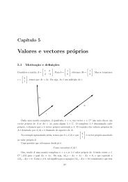
Retratos <strong>de</strong> fases <strong>do</strong> pêndulo matemático e <strong>do</strong> oscila<strong>do</strong>r harmónico.
6 EDOS LINEARES DE PRIMEIRA ORDEM 22<br />
6 EDOs lineares <strong>de</strong> primeira or<strong>de</strong>m<br />
1. (EDOs lineares <strong>de</strong> primeira or<strong>de</strong>m) A solução <strong>de</strong> uma EDO linear <strong>de</strong> primeira or<strong>de</strong>m<br />
ẋ + p(t) x = q(t) ,<br />
com condição inicial x(t 0 ) = x 0 , po<strong>de</strong> ser <strong>de</strong>termina<strong>da</strong> pelos seguintes <strong>do</strong>is passos: <strong>de</strong>terminar<br />
uma solução não-trivial y(t) <strong>da</strong> equação homogénea associa<strong>da</strong> ẏ + p(t) y = 0, substituir a<br />
conjetura x(t) = λ(t)y(t) na equação não-homogénea e resolver para λ(t). O resulta<strong>do</strong> é<br />
ẋ + p(t)x = q(t) , x(t 0 ) = x 0 ⇒ x(t) = e − R ( t<br />
p(u) du t 0 x 0 + ∫ R<br />
t s<br />
)<br />
p(u) t<br />
t 0<br />
e<br />
du 0 q(s)ds .<br />
• Mostre que se x 1 (t) e x 2 (t) são duas soluções <strong>da</strong> EDO linear <strong>de</strong> primeira or<strong>de</strong>m ẋ +<br />
p(t)x = q(t), então a diferença y(t) = x 1 (t)−x 2 (t) é uma solução <strong>da</strong> equação homogénea<br />
associa<strong>da</strong>, ẏ + p(t)y = 0.<br />
• Deduza que a solução geral <strong>de</strong> ẋ + p(t)x = q(t) po<strong>de</strong> ser representa<strong>da</strong> como uma soma<br />
x(t) = y(t) + z(t) ,<br />
on<strong>de</strong> y(t) = y(0)e − R t<br />
p(u)du t 0 é a solução geral <strong>da</strong> equação homogénea associa<strong>da</strong> e z(t) é<br />
uma solução particular, por exemplo a solução z(t) = e − R ( t<br />
p(u)du<br />
∫ R<br />
t t s<br />
)<br />
0 t<br />
t 0<br />
e<br />
p(u)du 0 q(s) ds<br />
com condição inicial nula.<br />
• Determine a solução geral <strong>da</strong>s EDOs lineares <strong>de</strong> primeira or<strong>de</strong>m<br />
2ẋ − 6x = e 2t ẋ + 2x = t ẋ + x/t 2 = 1/t 2 ẋ + tx = t 2<br />
<strong>de</strong>fini<strong>da</strong>s em oportunos intervalos <strong>da</strong> recta real.<br />
• Resolva os seguintes problemas <strong>de</strong> Cauchy nos intervalos indica<strong>do</strong>s:<br />
2ẋ − 3x = e 2t t ∈ (−∞, ∞) com x(0) = 1<br />
ẋ + x = e 3t t ∈ (−∞, ∞) com x(1) = 2<br />
tẋ − x = t 3 t ∈ (0, ∞) com x(1) = 3<br />
ẋ + tx = t 3 t ∈ (−∞, ∞) com x(0) = 0<br />
dr/dθ + r tan θ = cos θ t ∈ (−π/2, π/2) com r(0) = 1<br />
2. (que<strong>da</strong> livre com atrito) Um mo<strong>de</strong>lo mais realista <strong>da</strong> que<strong>da</strong> livre <strong>de</strong> uma partícula próxima<br />
<strong>da</strong> superfície terrestre <strong>de</strong>ve ter em conta a resistência <strong>do</strong> ar. A resistência po<strong>de</strong> ser mo<strong>de</strong>la<strong>da</strong><br />
como sen<strong>do</strong> uma força proporcional e contrária à veloci<strong>da</strong><strong>de</strong>, assim que a equação <strong>de</strong> Newton<br />
escreve-se<br />
m¨q = −γ ˙q − mg<br />
on<strong>de</strong> γ > 0 é um coeficiente <strong>de</strong> atrito. Portanto, a veloci<strong>da</strong><strong>de</strong> v := ˙q satisfaz a EDO linear<br />
<strong>de</strong> primeira or<strong>de</strong>m<br />
m ˙v = −γv − mg .<br />
• Resolva o problema com condição inicial v(0) = 0.<br />
• Mostre que a veloci<strong>da</strong><strong>de</strong> v(t) converge para um valor assimptótico v quan<strong>do</strong> t → ∞,<br />
in<strong>de</strong>pen<strong>de</strong>ntemente <strong>do</strong> seu valor inicial, e <strong>de</strong>termine este valor.<br />
• Utilize a solução encontra<strong>da</strong> para <strong>de</strong>terminar a trajectória q(t) com condição inicial<br />
q(0) = s.
6 EDOS LINEARES DE PRIMEIRA ORDEM 23<br />
3. (circuito RL) A corrente I(t) num circuito RL, <strong>de</strong> resistência R e indutância L, é <strong>de</strong>termina<strong>da</strong><br />
pela EDO<br />
LI ˙ + RI = V (t)<br />
on<strong>de</strong> V (t) é a tensão que alimenta o circuito.<br />
• Escreva a solução geral como função <strong>da</strong> corrente inicial I(0) = I 0 .<br />
• Resolva a equação para um circuito alimenta<strong>do</strong> com tensão constante V (t) = E. Esboce<br />
a representação gráfica <strong>de</strong> algumas <strong>da</strong>s soluções e diga o que acontece para gran<strong>de</strong>s<br />
intervalos <strong>de</strong> tempo.<br />
• Resolva a equação para um circuito alimenta<strong>do</strong> com uma tensão alterna<strong>da</strong> V (t) =<br />
E sin(ωt). Verifique que a solução com I(0) = 0 é<br />
I(t) =<br />
on<strong>de</strong> φ é uma fase que <strong>de</strong>pen<strong>de</strong> <strong>de</strong> ω, L e R.<br />
E<br />
EωL<br />
√ sin (ωt − φ) +<br />
R2 + ω 2 L2 R 2 + ω 2 L 2 e− R L t<br />
4. (lei <strong>do</strong> arrefecimento <strong>de</strong> Newton) A temperatura T (t) no instante t <strong>de</strong> um corpo num meio<br />
ambiente cuja temperatura no instante t é M(t) segue a lei <strong>do</strong> arrefecimento <strong>de</strong> Newton<br />
˙ T = −k (T − M(t)) ,<br />
on<strong>de</strong> k > 0 é uma constante positiva (que <strong>de</strong>pen<strong>de</strong> <strong>do</strong> material <strong>do</strong> corpo).<br />
• Escreva a solução geral como função <strong>da</strong> temperatura inicial T (0) = T 0 e <strong>do</strong>s valores <strong>da</strong><br />
função M(τ) com 0 ≤ τ ≤ t.<br />
• Determine a solução assimptótica (ou seja, quan<strong>do</strong> t é gran<strong>de</strong>) T (t) quan<strong>do</strong> M(t) =<br />
M sin(ωt).<br />
• Resolva a equação quan<strong>do</strong> a temperatura <strong>do</strong> meio ambiente é manti<strong>da</strong> constante M(t) =<br />
M. Esboce a representação gráfica <strong>de</strong> algumas <strong>da</strong>s soluções e diga o que acontece para<br />
gran<strong>de</strong>s intervalos <strong>de</strong> tempo.<br />
• Uma chávena <strong>de</strong> café, com temperatura inicial <strong>de</strong> 100 o C, é coloca<strong>da</strong> numa sala cuja<br />
temperatura é <strong>de</strong> 20 o C. Saben<strong>do</strong> que o café atinge uma temperatura <strong>de</strong> 60 o C em 10<br />
minutos, <strong>de</strong>termine a constante k <strong>do</strong> café e o tempo necessário para o café atingir a<br />
temperatura <strong>de</strong> 40 o C.<br />
5. (equações <strong>de</strong> Bernoulli) Uma EDO <strong>da</strong> forma<br />
ẋ + p(t) x = q(t) x n ,<br />
on<strong>de</strong> p e q são funções contínuas num intervalo I ⊂ R e n ≠ 0, 1 (caso contrário trata-se <strong>de</strong><br />
uma normal equação linear <strong>da</strong> primeira or<strong>de</strong>m), é dita equação <strong>de</strong> Bernoulli.<br />
• Verifique que x(t) = 0 é uma solução <strong>de</strong> equilíbrio <strong>da</strong> equação <strong>de</strong> Bernoulli.<br />
• Seja k = 1 − n. Mostre que x(t) é uma solução positiva <strong>da</strong> equação <strong>de</strong> Bernoulli com<br />
condição inicial x(t 0 ) = x 0 > 0 se e só se a função y(t) = x(t) k é uma solução <strong>da</strong> EDO<br />
linear<br />
ẏ + k p(t) y = k q(t)<br />
com condição inicial y(t 0 ) = (x 0 ) 1/k .<br />
• Resolva os seguintes problemas <strong>de</strong> Cauchy para equações <strong>de</strong> Bernoulli:<br />
ẋ + x = x 2 (cos t − sin t) t ∈ (−∞, ∞) com x(1) = 2<br />
tẋ + e t2 x = x 2 log t t ∈ (0, ∞) com x(3) = 0<br />
ẋ − x/t = t √ x t ∈ (0, ∞) com x(1) = 1
7 EDOS SEPARÁVEIS E HOMOGÉNEAS 24<br />
7 EDOs separáveis e homogéneas<br />
1. (produto direto <strong>de</strong> EDOs) As soluções <strong>do</strong> sistema autónomo<br />
{ ẋ = f(x)<br />
ẏ = g(y)<br />
(produto direto <strong>da</strong>s EDOs ẋ = f(x) e ẏ = g(y)) são os caminhos t ↦→ (x(t), y(t)), on<strong>de</strong> x(t) e<br />
y(t) são as soluções <strong>da</strong>s EDOs autónomas ẋ = f(x) e ẏ = g(y), respetivamente. A curva <strong>de</strong><br />
fases que passa pelo ponto (x 0 , y 0 ) ∈ R 2 , on<strong>de</strong> f(x 0 ) ≠ 0 (ou on<strong>de</strong> g(y 0 ) ≠ 0), é (localmente)<br />
o gráfico <strong>de</strong> uma função x ↦→ y(x) (ou y ↦→ x(y)) que satisfaz a EDO<br />
dy<br />
dx = g(y)<br />
f(x)<br />
(<br />
ou<br />
dx<br />
dy = f(y)<br />
g(x)<br />
• Determine as soluções e as curvas <strong>de</strong> fases <strong>do</strong> sistema<br />
{ ẋ = x<br />
ẏ = λy<br />
quan<strong>do</strong> λ = 0, ±1, 2, . . . e quan<strong>do</strong> λ = 1/2, 1/3, . . . .<br />
2. (EDOs separáveis) A solução <strong>da</strong> uma EDO separável<br />
dy<br />
dx = g(y)<br />
f(x) .<br />
com condição inicial y(x 0 ) = y 0 tal que f(x 0 ) ≠ 0 e g(y 0 ) ≠ 0, é <strong>da</strong><strong>da</strong> em forma implícita<br />
por<br />
dy<br />
dx = g(y)<br />
f(x) , y(x 0) = y 0<br />
⇒<br />
∫ x<br />
x 0<br />
)<br />
.<br />
dξ<br />
f(ξ) = ∫ y<br />
y 0<br />
dη<br />
g(η)<br />
• Resolva as seguintes EDOs separáveis <strong>de</strong>fini<strong>da</strong>s em oportunos <strong>do</strong>mínios.<br />
dy<br />
dx = −x y<br />
dy<br />
dx = kxα y β<br />
dy<br />
dx = sin x<br />
sin y<br />
ẋ = tx 3 tẋ + t = t 2 ẋ = t 3 /x 2 xẋ = e x+3t2 t<br />
ẋ = t − 1 x − 1<br />
x 2 ẋ + x − x2<br />
dy<br />
t t 2 = 0<br />
dx = −x y<br />
(<br />
t 2 + 1 ) ẋ = 2tx ẋ = t ( x 2 − x ) ẋ = e t−x ,<br />
3. (homotetias e funções homogéneas) As homotetias (positivas) <strong>do</strong> espaço Euclidiano R n são<br />
as transformações x ↦→ λx, com λ ∈ R + := (0, ∞). Uma função f : D → R (ou um campo<br />
vetorial F : D → R m ), <strong>de</strong>fini<strong>da</strong> num <strong>do</strong>mínio “homogéneo” (i.e. invariante para homotetias)<br />
D ⊂ R n \{0}, é dita homogénea <strong>de</strong> grau k se<br />
f(λx) = λ k f(x) ∀ λ ∈ R + e ∀ x ∈ D ,<br />
e é dita homogénea (<strong>de</strong> grau 0) se é invariante para homotetias, ou seja, se<br />
f(λx) = f(x) ∀ λ ∈ R + e ∀ x ∈ D .<br />
O teorema <strong>de</strong> Euler afirma que uma função diferenciável f : D ⊂ R n \{0} → R é homogénea<br />
<strong>de</strong> grau k se e só se 〈x, ∇f(x)〉 = k f(x) para to<strong>do</strong>s os pontos x ∈ D.<br />
• Determine os polinómios homogéneos <strong>de</strong> grau 1, <strong>de</strong> grau 2 e <strong>de</strong> grau 3 no plano R 2 .<br />
• Mostre que as únicas funções homogéneas e contínuas <strong>de</strong>fini<strong>da</strong> em to<strong>do</strong> o espaço R n são<br />
as constantes (observe que as funções homogéneas são constantes ao longo <strong>da</strong>s semi-retas<br />
que saem <strong>da</strong> origem, logo, se a origem está no <strong>do</strong>mínio <strong>da</strong> função . . . ).
7 EDOS SEPARÁVEIS E HOMOGÉNEAS 25<br />
• Determine o grau <strong>de</strong> homogenei<strong>da</strong><strong>de</strong> <strong>do</strong>s campos <strong>de</strong> forças elástico e gravitacional/elétrico,<br />
<strong>de</strong>fini<strong>do</strong>s por<br />
F(r) = −r e F(r) = − r<br />
‖r‖ 3 ,<br />
respetivamente (o segun<strong>do</strong> <strong>de</strong>fini<strong>do</strong> para r ∈ R 3 \{0}).<br />
• Diga se as seguintes funções f(x, y), <strong>de</strong>fini<strong>da</strong>s em oportunos <strong>do</strong>mínios <strong>do</strong> plano, são<br />
homogéneas:<br />
x/y e x−y x 2 − xy<br />
xy + 3y 2 sin(y) cos(x)<br />
4. (EDOs homogéneas) Uma EDO homogénea é uma equação diferencial<br />
ẋ = v(t, x)<br />
<strong>de</strong>fini<strong>da</strong>, num <strong>do</strong>mínio D ⊂ R 2 <strong>do</strong> plano <strong>de</strong> coor<strong>de</strong>na<strong>da</strong>s (t, x), por um campo <strong>de</strong> direções<br />
homogéneo, ou seja, tal que v(λt, λx) = v(t, x) para to<strong>do</strong>s os λ > 0. As homotetias (t, x) ↦→<br />
(λt, λx), com λ ∈ R + , enviam curvas integrais <strong>de</strong> uma EDO homogénea em curvas integrais.<br />
A mu<strong>da</strong>nça <strong>de</strong> variável y(t) := x(t)/t, num <strong>do</strong>mínio on<strong>de</strong> t > 0 ou t < 0, transforma uma<br />
EDO homogénea ẋ = v(t, x) numa EDO separável y + tẏ = v(1, y). Ou seja,<br />
ẋ = v(1, x/t) ⇒ y + tẏ = v(1, y) se y = x/t<br />
• Seja ẋ = v(t, x). uma EDO homogénea. Mostre que, se ϕ(t) é uma solução e λ ∈ R,<br />
então também φ(t) := λ · ϕ (t/λ) é uma solução.<br />
• Seja ϕ(t) uma solução <strong>da</strong> EDO homogénea ẋ = v(t, x) tal que ϕ(1) = 5 e ϕ(2) = 7. Se<br />
φ(t) é uma outra solução tal que φ(3) = 15, quanto vale φ(6)<br />
• Resolva as seguintes EDOs homogéneas<br />
ẋ = −t/x<br />
ẋ = x − t<br />
x + t<br />
ẋ = 1 + x/t<br />
ẋ = x/t ẋ = 2 t x ex/t + x dy<br />
= y/x + sin(y/x) ,<br />
t dx<br />
<strong>de</strong>fini<strong>da</strong>s em oportunos <strong>do</strong>mínios, e esboce a representação gráfica <strong>de</strong> algumas <strong>da</strong>s<br />
soluções.<br />
5. (equação <strong>de</strong> Newton com forças homogéneas) [Ar89, LL78] Consi<strong>de</strong>re a equação <strong>de</strong> Newton<br />
m¨r = F(r)<br />
para a trajetória t ↦→ r(t) ∈ R 3 <strong>de</strong> uma partícula sujeita a una força F(r) homogénea <strong>de</strong><br />
grau k, ou seja tal que F(λr) = λ k F(r) para to<strong>do</strong>s os λ > 0 e to<strong>do</strong> os pontos r ∈ R 3 \{0}.<br />
As “quase-homotetia” (t, r) ↦→ (λ α t, λ β r), com λ > 0, enviam curvas integrais em curvas<br />
integrais se os “pesos” α e β satisfazem a relação β(1 − k) = 2α. Em particular, uma órbita<br />
fecha<strong>da</strong> <strong>de</strong> dimensão linear L e perío<strong>do</strong> <strong>de</strong> revolução T é envia<strong>da</strong> numa órbita fecha<strong>da</strong> <strong>de</strong><br />
dimensão linear L ′ = λ β L e perío<strong>do</strong> <strong>de</strong> revolução T ′ = λ α T , e portanto o quociente T β /L α<br />
é constante.<br />
• Consi<strong>de</strong>re uma força constante (e.g. a gravi<strong>da</strong><strong>de</strong> próximo <strong>da</strong> superfície <strong>da</strong> terra)<br />
F (x) ∝ 1 ,<br />
e <strong>de</strong>termine a relação entre espaço percorri<strong>do</strong> e tempo necessário.<br />
• Consi<strong>de</strong>re a forçã elástica (e.g. lei <strong>de</strong> Hooke, oscila<strong>do</strong>r harmónico)<br />
F (x) ∝ −x ,<br />
e <strong>de</strong>duza que os perío<strong>do</strong>s <strong>da</strong>s órbitas fecha<strong>da</strong>s não <strong>de</strong>pen<strong>de</strong>m <strong>da</strong>s amplitu<strong>de</strong>s <strong>da</strong>s oscilações.
7 EDOS SEPARÁVEIS E HOMOGÉNEAS 26<br />
• Consi<strong>de</strong>re uma força elástica “fraca”<br />
F (x) ∝ −x 3 ,<br />
Determine o perío<strong>do</strong> <strong>da</strong>s pequenas oscilações em quanto função <strong>da</strong> amplitu<strong>de</strong>.<br />
• Consi<strong>de</strong>re a força gravitacional<br />
F(r) ∝ −<br />
r<br />
‖r‖ 3 ,<br />
e <strong>de</strong>duza a terceira lei <strong>de</strong> Kepler 14 : “os quadra<strong>do</strong>s <strong>do</strong>s perío<strong>do</strong>s <strong>de</strong> revolução T são<br />
proporcionais aos cubos <strong>da</strong>s distâncias médias L <strong>do</strong> Sol aos planetas, ou seja, T 2 = kL 3 ,<br />
on<strong>de</strong> k é uma constante”.<br />
14 Johannes Kepler, Harmonices mundi, 1619.
8 EDOS EXATAS E CAMPOS CONSERVATIVOS 27<br />
8 EDOs exatas e campos conservativos<br />
1. (EDOs exatas, diferenciais exatos e campos conservativos) O differencial p(x, y)dx+q(x, y)dy<br />
é dito exato no <strong>do</strong>mínio D ⊂ R 2 se existe uma função U : D → R <strong>de</strong> classe C 1 , dita primitiva,<br />
tal que dU = pdx + qdy, ou seja,<br />
∂U<br />
∂x = p e ∂U<br />
∂y = q .<br />
A primitiva é também dita potencial <strong>do</strong> campo <strong>de</strong> vetores F := −∇U = −(p, q). As curvas<br />
<strong>de</strong> nível regulares<br />
Σ c := {(x, y) ∈ D ⊂ R 2 t.q. U(x, y) = c} ,<br />
com c ∈ R valor regular <strong>de</strong> U (i.e. tal que ∇U ≠ 0 nos pontos <strong>de</strong> Σ c ), ortogonais ao campo<br />
<strong>de</strong> vetores F em to<strong>do</strong>s os pontos <strong>de</strong> D, são as soluções <strong>da</strong> equação diferencial exata<br />
p(x, y) dx + q(x, y) dy = 0 .<br />
O teorema <strong>de</strong> Euler-Poincaré afirma que o diferencial p(x, y)dx + q(x, y)dy, <strong>de</strong>fini<strong>do</strong> num<br />
<strong>do</strong>mínio convexo 15 (é suficiente que seja “simplesmente conexo”) D ⊂ R 2 , é exato se e só se<br />
é “fecha<strong>do</strong>”, i.e. se<br />
( ∂q<br />
∂x − ∂p )<br />
dx ∧ dy = 0<br />
∂y<br />
ou seja,<br />
e, se isto acontecer, um potencial é <strong>da</strong><strong>do</strong> pelo integral <strong>de</strong> linha<br />
U(x, y) = ∫ p(x, y) dx + q(x, y) dy<br />
γ<br />
∂p<br />
∂y = ∂q<br />
∂x<br />
on<strong>de</strong> γ : [0, 1] → D ⊂ R 2 é um caminho diferenciável entre γ(0) = (x 0 , y 0 ) e γ(1) = (x, y).<br />
• Diga quais <strong>do</strong>s seguintes diferenciais,<br />
dx + dy<br />
e xy dx + e xy dy<br />
(2y + 3x) dx + (y + 2x) dy<br />
x<br />
dy + (1 + log y) dx ,<br />
y<br />
<strong>de</strong>fini<strong>do</strong>s em oportunos rectângulos, são exatos, e esboce algumas curvas integrais <strong>da</strong><br />
correspon<strong>de</strong>nte equação diferencial.<br />
• Diga quais <strong>da</strong>s seguintes EDOs<br />
5 + 3 dx<br />
dt = 0<br />
dx<br />
(x − t)<br />
dt + ex = 0<br />
1<br />
x + t − t dx<br />
x 2 dt = 0<br />
(<br />
4x + 3y<br />
2 ) +2xy dy<br />
dx = 0 2x2 +4t 3 +(4tx + 1) dx<br />
dt = 0<br />
(<br />
r 2 + 1 ) cos θ+2r sin θ dr<br />
dθ = 0 ,<br />
<strong>de</strong>fini<strong>da</strong>s em oportunos retângulos, são exatas, e resolva-as.<br />
• Verifique que, se a forma pdx + qdy está <strong>de</strong>fini<strong>da</strong> numa bola B R (0) <strong>de</strong> raio 0 < R ≤ ∞,<br />
e satisfaz a condição ∂p<br />
∂y<br />
= ∂q<br />
∂x<br />
<strong>do</strong> teorema <strong>de</strong> Euler-Poincaré, então uma primitiva é<br />
também <strong>da</strong><strong>da</strong> pelo integral<br />
U(x, y) =<br />
∫ 1<br />
0<br />
(x p(tx, ty) + y q(tx, ty)) dt .<br />
15 Uma região D ⊂ R n é convexa se a, b ∈ D implica ta + (1 − t)b ∈ D para to<strong>do</strong>s os t ∈ [0, 1].
8 EDOS EXATAS E CAMPOS CONSERVATIVOS 28<br />
2. (fatores integrantes) Um diferencial arbitrário pdx + qdy po<strong>de</strong> ser transforma<strong>do</strong> num diferencial<br />
exato (pµ)dx + (qµ)dy por meio <strong>de</strong> um fator integrante, uma função µ(x, y) tal que<br />
∂(µp)<br />
∂y<br />
= ∂(µq)<br />
∂x .<br />
Não existem méto<strong>do</strong>s gerais para <strong>de</strong>terminar fatores integrantes. No entanto, fatores integrantes<br />
que <strong>de</strong>pen<strong>de</strong>m <strong>de</strong> apenas uma variável po<strong>de</strong>m ser <strong>de</strong>termina<strong>do</strong>s, quan<strong>do</strong> existem!,<br />
por meio <strong>de</strong> uma integração. Por exemplo, um fator integrante µ(x) é solução <strong>da</strong> EDO linear<br />
<strong>de</strong> primeira or<strong>de</strong>m<br />
( )<br />
µ ∂p<br />
∂y = µ′ q + µ ∂q<br />
∂x<br />
ou seja, µ ′ /µ = 1 ∂p<br />
q ∂y − ∂q<br />
∂x<br />
<strong>de</strong>s<strong>de</strong> que 1 q<br />
( )<br />
∂p<br />
∂y − ∂q<br />
∂x<br />
não <strong>de</strong>pen<strong>de</strong> <strong>de</strong> y.<br />
• Consi<strong>de</strong>re as equações diferenciais<br />
(<br />
4x + 3y<br />
2 ) + 2xy dy<br />
dx = 0<br />
<strong>do</strong>n<strong>de</strong><br />
(<br />
2x 2 + y ) + ( x 2 y − x ) dy<br />
dx = 0 .<br />
R 1<br />
µ = e<br />
q ( ∂p<br />
∂y − ∂x)dx<br />
∂q<br />
Mostre que não são exactas.<br />
Determine um fator integrante <strong>da</strong> forma x n com n inteiro. Multiplique as equações<br />
pelos respetivos fatores integrantes e resolva as equações resultantes.<br />
3. (curvas ortogonais) Se a famíia C <strong>de</strong> curvas no plano é <strong>de</strong>fini<strong>da</strong> como sen<strong>do</strong> as curvas integrais<br />
<strong>da</strong> equação diferencial<br />
p(x, y) dx + q(x, y) dy = 0 ,<br />
então a família C ⊥ <strong>de</strong> curvas ortogonais é composta pelas curvas integrais <strong>da</strong> equação diferencial<br />
p(x, y) dy − q(x, y) dx = 0 .<br />
(o opera<strong>do</strong>r que envia o diferencial ω = pdx + qdx no diferencial ∗ω = pdy − qdx é chama<strong>do</strong><br />
“Hodge star operator” no plano euclidiano).<br />
• Determine e esboce as curvas ortogonais . . .<br />
. . . à família <strong>de</strong> círculos x 2 + y 2 = c,<br />
. . . à família <strong>de</strong> hipérboles xy = c,<br />
. . . e à família <strong>de</strong> parábolas y 2 = cx.<br />
4. (campos conservativos) O trabalho efectua<strong>do</strong> pelo campo <strong>de</strong> vectores/forças F(x, y) ∈ R 2 ou<br />
F(x, y, z) ∈ R 3 , <strong>de</strong>fini<strong>do</strong> num <strong>do</strong>mínio D ⊂ R 2 ou R 3 , ao longo <strong>do</strong> caminho diferenciável<br />
γ : [0, 1] → D é o integral <strong>de</strong> linha<br />
∫<br />
Work[F, γ] := 〈F(γ(t)), ˙γ(t)〉 dt .<br />
γ<br />
O campo <strong>de</strong> vectores F é conservativo se o trabalho apenas <strong>de</strong>pen<strong>de</strong> <strong>do</strong>s pontos inicial e<br />
final <strong>do</strong> caminho, ou seja, se o campo admite um potencial, i.e. uma função diferenciável<br />
U : D → R tal que F = −∇U, e portanto<br />
∫<br />
〈F(γ(t)), ˙γ(t)〉 dt = U(γ(1)) − U(γ(0)) .<br />
• Diga quais <strong>do</strong>s seguintes campos <strong>de</strong> forças<br />
γ<br />
F(x, y) = (3, 2) F(x, y) = (x, y) F(x, y) = (x, −y)<br />
( )<br />
x<br />
F(x, y) = (−y, x) F(x, y) =<br />
x 2 + y 2 , y<br />
x 2 + y 2 ,<br />
<strong>de</strong>fini<strong>do</strong>s em oportunos <strong>do</strong>mínios <strong>do</strong> plano, são conservativos, e <strong>de</strong>termine as curvas<br />
equipotenciais.
8 EDOS EXATAS E CAMPOS CONSERVATIVOS 29<br />
• Diga se o campo <strong>de</strong> forças<br />
F(x, y) =<br />
( )<br />
−y<br />
x 2 + y 2 , x<br />
x 2 + y 2 ,<br />
<strong>de</strong>fini<strong>do</strong> em R\{(0, 0)}, é conservativo.
9 EDOS LINEARES HOMOGÉNEAS COM COEFICIENTES CONSTANTES 30<br />
9 EDOs lineares homogéneas com coeficientes constantes<br />
1. (equação <strong>de</strong> Newton num potencial quadrático) Consi<strong>de</strong>re a equação <strong>de</strong> Newton<br />
¨q = −βq<br />
que <strong>de</strong>termina a trajetória t ↦→ q(t) ∈ R <strong>de</strong> uma partícula (<strong>de</strong> massa m = 1) num potencial<br />
quadrático U(q) = 1 2 βq2 .<br />
• Verifique que q(t) = 0 é uma solução <strong>de</strong> equilíbrio.<br />
• Verifique que, se β = 0, as soluções <strong>da</strong> equação <strong>de</strong> Newton (<strong>da</strong> partícula livre)<br />
¨q = 0<br />
são q(t) = a + bt, com a, b ∈ R constantes arbitrárias.<br />
• Verifique que, se β = −k 2 < 0, as soluções <strong>da</strong> equação <strong>de</strong> Newton<br />
¨q = k 2 q<br />
são q(t) = ae kt + be −kt , com a, b ∈ R constantes arbitrárias.<br />
• Verifique que, se β = ω 2 > 0, as soluções <strong>da</strong> equação (<strong>do</strong> oscila<strong>do</strong>r harmónico)<br />
¨q = −ω 2 q<br />
são q(t) = a cos(ωt) + b sin(ωt), com a, b ∈ R constantes arbitrárias.<br />
2. (partícula num potencial quadrático com atrito) A função q(t) := e −αt y(t) é uma solução<br />
<strong>da</strong> equação <strong>de</strong> Newton (<strong>de</strong> uma partícula num potencial quadrático U(q) = 1 2 βq2 com uma<br />
força <strong>de</strong> atrito −2αq, se α > 0),<br />
¨q = −2α ˙q − βq ,<br />
sse y(t) é uma solução <strong>da</strong> equação <strong>de</strong> Newton<br />
ÿ = −δy<br />
(<strong>de</strong> uma partícula num potencial quadrático U(y) = 1 2 δy2 ), on<strong>de</strong> δ := β − α 2 .<br />
• Verifique a afirmação acima.<br />
• Determine a solução geral <strong>da</strong> equação.<br />
• Existem soluções <strong>de</strong> equilíbrio<br />
3. (EDOs lineares homogéneas com coeficientes constantes, polinómio característico) A conjectura<br />
x(t) = e zt é uma solução (complexa) <strong>da</strong> EDO linear homogénea <strong>de</strong> segun<strong>da</strong> or<strong>de</strong>m com<br />
coeficientes constantes<br />
ẍ + 2αẋ + βx = 0<br />
se z é igual a uma <strong>da</strong>s raizes z ± = −α ± √ α 2 − β <strong>do</strong> polinómio caractéristico<br />
P (z) := z 2 + 2αz + β .<br />
Duas soluções (reais) in<strong>de</strong>pen<strong>de</strong>ntes po<strong>de</strong>m ser obti<strong>da</strong>s calculan<strong>do</strong> a parte real e a parte<br />
imaginária <strong>da</strong>s soluções complexas, e são<br />
e (−α+k)t e e (−α−k)t se z ± = −α ± k , com k > 0 (raizes reais e distintas)<br />
e −αt cos(ωt) e e −αt sin(ωt) se z ± = −α ± iω , com ω > 0 (raizes complexas conjuga<strong>da</strong>s)<br />
e −αt e te −αt se z ± = −α (raiz dupla)<br />
O espaço <strong>da</strong>s soluções (reais) <strong>da</strong> EDO homogénea ẍ + 2αẋ + βx = 0 é um espaço linear<br />
H ≃ R 2 , <strong>de</strong> dimensão 2. Se φ + (t) e φ − (t) formam uma base <strong>de</strong> H, então a “solução geral” é<br />
x(t) = c + φ + (t) + c − φ − (t), on<strong>de</strong> c ± ∈ R são constantes arbitrárias.
9 EDOS LINEARES HOMOGÉNEAS COM COEFICIENTES CONSTANTES 31<br />
• Verifique que o espaço <strong>da</strong>s soluções <strong>da</strong> EDO homogénea ẍ + 2αẋ + βx = 0 é um espaço<br />
linear, ou seja, que uma combinação linear c + x + (t) + c − x − (t), com c ± ∈ R, <strong>de</strong> soluções<br />
x ± (t) é uma solução.<br />
• Determine a solução geral <strong>da</strong>s seguintes EDOs homogéneas:<br />
ẍ − 2x = 0 ẍ + π 2 x = 0 3ẍ + ẋ = 0 ẍ − ẋ = 0<br />
ẍ + 2ẋ − x = 0 ẍ + 2ẋ + x = 0 ẍ + 4ẋ + 5x = 0 ẍ − 4ẋ + x = 0 .<br />
• Resolva os seguintes problemas <strong>de</strong> Cauchy:<br />
ẍ + 2x = 0 com x(0) = 0 e ẋ(0) = 2<br />
ẍ + ẋ = 0 com x(0) = 1 e ẋ(0) = 0<br />
ẍ + 4ẋ + 5x = 0<br />
com x(0) = 2 e ẋ(0) = −1<br />
ẍ − 17ẋ + 13x = 0 com x(3) = 0 e ẋ(3) = 0<br />
ẍ − 2ẋ − 2x = 0 com x(0) = 0 e ẋ(0) = 9<br />
ẍ − 4ẋ − x = 0 com x(1) = 2 e ẋ(1) = 1 .<br />
• Determine umas equações diferenciais <strong>de</strong> segun<strong>da</strong> or<strong>de</strong>m que admitem como soluções os<br />
seguintes pares <strong>de</strong> funções:<br />
e 2t e e −2t , e −t sin(2πt) e e −t cos(2πt) , sinh(t) e cosh(t) ,<br />
e −3t e te −3t , sin(2t + 1) e cos(2t + 2) , 3 e 5t .<br />
4. (in<strong>de</strong>pendência linear e Wronskiano) O (<strong>de</strong>terminante) Wronskiano entre as funções f(t) and<br />
g(t), <strong>de</strong>fini<strong>da</strong>s num intervalo I ⊂ R, é a função<br />
(<br />
f(t) f(t) ˙<br />
W f,g (t) := <strong>de</strong>t<br />
g(t) ġ(t)<br />
)<br />
= f(t)ġ(t) − ˙ f(t)g(t)<br />
Se W f,g (t) = 0 para to<strong>do</strong>s os tempos t ∈ I então o quociente g/f (ou f/g) é constante<br />
no intervalo I. Consequentemente, se f(t) e g(t) são linearmente in<strong>de</strong>pen<strong>de</strong>ntes, então o<br />
Wronskiano W f,g (t) ≠ 0 em algum ponto t ∈ I.<br />
Se φ + e φ − são duas soluções <strong>da</strong> mesma EDO linear ẍ + p(t)ẋ + q(t)x = 0, <strong>de</strong>fini<strong>da</strong>s num<br />
intervalo I ⊂ R, e t 0 ∈ I, então o Wronskiano satisfaz a i<strong>de</strong>nti<strong>da</strong><strong>de</strong> <strong>de</strong> Abel<br />
W φ+,φ −<br />
(t) = W φ+,φ −<br />
(t 0 ) · e − R t<br />
t 0 p(s)ds .<br />
Portanto, φ + e φ − são linearmente in<strong>de</strong>pen<strong>de</strong>nte se e só se W φ+,φ −<br />
(t) ≠ 0 num ponto (e<br />
portanto em to<strong>do</strong>s os pontos) t ∈ I.<br />
• Sejam φ + e φ − duas soluções <strong>da</strong> EDO linear ẍ + p(t)ẋ + q(t)x = 0. Calcule a <strong>de</strong>riva<strong>da</strong><br />
<strong>de</strong> W φ+,φ −<br />
(t), e <strong>de</strong>duza a i<strong>de</strong>nti<strong>da</strong><strong>de</strong> <strong>de</strong> Abel.<br />
• Calcule<br />
W e −αt ,te −αt , W e −αt e kt ,e −αt e −kt and W e −αt sin(ωt),e −αt cos(ωt) .<br />
5. (equação <strong>de</strong> Schrödinger estacionária) Consi<strong>de</strong>re a equação <strong>de</strong> Schrödinger estacionária<br />
− 2 d 2 ψ<br />
2m dx 2 = Eψ<br />
para a função <strong>de</strong> on<strong>da</strong> ψ(x) <strong>de</strong> uma partícula livre, on<strong>de</strong> m é a massa <strong>da</strong> partícula, = h/2π<br />
é a constante <strong>de</strong> Planck reduzi<strong>da</strong>, h ≃ 6.262... × 10 −34 J·s.
9 EDOS LINEARES HOMOGÉNEAS COM COEFICIENTES CONSTANTES 32<br />
• Determine para quais valores E <strong>da</strong> energia existem soluções não triviais <strong>da</strong> equação no<br />
intervalo x ∈ [0, l] com condições <strong>de</strong> fronteira ψ(0) = 0 e ψ(l) = 0 (partícula numa<br />
caixa).<br />
6. (EDOs equidimensionais) Uma equação diferencial <strong>da</strong> forma<br />
ax 2 d2 y dy<br />
+ bx<br />
dx2 dx + cy = 0<br />
é dita equidimensional (é invariante pela transformação x ↦→ λx com λ > 0).<br />
• Mostre que a substituição x = e t transforma a equação equidimensional para y(x) numa<br />
equação com coeficientes constantes para z(t) := y(x(t)).<br />
• Resolva a equação<br />
na semirecta x > 0.<br />
x 2 d2 y<br />
dx 2 + x dy<br />
dx − 4y = 0 ,<br />
7. (EDOs <strong>de</strong> Riccati) Uma equação diferencial <strong>da</strong> forma<br />
é dita equação <strong>de</strong> Riccati.<br />
• Mostre que a variável x(t), tal que<br />
ÿ + p(t)y 2 + q(t)y + r(t) = 0<br />
ẋ = −p(t)y(t) ,<br />
satisfaz a EDO linear<br />
(<br />
ẍ + q(t) + ṗ(t) )<br />
ẋ + p(t)r(t)x = 0 .<br />
p(t)
10<br />
NÚMEROS COMPLEXOS E OSCILAÇÕES 33<br />
10 Números complexos e oscilações<br />
1. (o plano <strong>do</strong>s números complexos) O corpo <strong>do</strong>s números complexos é o conjunto C ≃ R 2<br />
<strong>do</strong>s pontos/números z = x + iy ≃ (x, y), com x, y ∈ R, muni<strong>do</strong> <strong>da</strong>s operações “soma” e<br />
“multiplicação”, <strong>de</strong>fini<strong>da</strong>s por<br />
(x 1 + iy 1 ) + (x 2 + iy 2 ) = (x 1 + x 2 ) + i(y 1 + y 2 )<br />
(que correspon<strong>de</strong> à soma <strong>do</strong>s vetores (x 1 , y 1 ) e (x 2 , y 2 ) <strong>do</strong> plano R 2 ) e<br />
(x 1 + iy 1 ) · (x 2 + iy 2 ) = (x 1 x 2 − y 1 y 2 ) + i(x 1 y 2 + x 2 y 1 ) .<br />
Em particular, se i := 0 + i · 1 ∈ C, então i · i = −1, ou seja, i = √ −1. O conjuga<strong>do</strong> <strong>de</strong><br />
z = x + iy é z := x − iy. O módulo <strong>de</strong> z = x + iy é<br />
|z| := √ zz = √ x 2 + y 2 .<br />
Os números reais<br />
x = R(z) := z + z e y = I(z) := z − z<br />
2<br />
2i<br />
são ditos parte real e parte imaginária <strong>do</strong> número complexo z = x + iy. A representação<br />
polar <strong>do</strong> número complexo z = x + iy ≃ (x, y) ∈ R 2 é<br />
z = ρ e iθ<br />
on<strong>de</strong> ρ = |z| ≥ 0 é o módulo, θ ∈ R é “um” argumento <strong>de</strong> z, ou seja, um “ângulo” arg(z) =<br />
θ + 2πn, com n ∈ Z, tal que x = ρ cos(θ) e y = ρ sin(θ), e o número complexo e iθ é <strong>de</strong>fini<strong>do</strong><br />
pela fórmula <strong>de</strong> Euler<br />
e iθ := cos(θ) + i sin(θ)<br />
• Verifique que o inverso multiplicativo <strong>de</strong> um número complexo z ≠ 0 é<br />
1/z = z/|z| 2<br />
• Represente na forma x + iy os seguintes números complexos<br />
1/i<br />
2 − i<br />
1 + i<br />
1 − i<br />
1 + i · i<br />
2 + i<br />
(1 − i3) 2<br />
• Resolva as seguintes equações<br />
z 2 − 2z + 2 = 0 z 2 + z + 1 = 0<br />
• Verifique que, se z 1 = ρ 1 e iθ1<br />
e z 2 = ρ 2 e iθ2 , então<br />
z 1 z 2 = ρ 1 ρ 2 e i(θ1+θ2)<br />
e<br />
z 1<br />
z 2<br />
= ρ 1<br />
ρ 2<br />
e i(θ1−θ2) (se ρ 2 ≠ 0) .<br />
Deduza que a multiplicação por z = ρe iθ , no plano C ≃ R 2 , correspon<strong>de</strong> a uma dilatação/contração<br />
por ρ e uma rotação <strong>de</strong> um ângulo θ. Em particular, a multiplicação<br />
por i = e iπ/2 é a “raiz quadra<strong>da</strong>” <strong>da</strong> inversão (x, y) ↦→ (−x, −y), ou seja, uma rotação<br />
<strong>de</strong> um ângulo π/2.<br />
• Use a fórmula <strong>de</strong> Euler para provar as fórmulas<br />
cos(θ ± φ) = cos(θ) cos(φ) ∓ sin(θ) sin(φ)<br />
e<br />
sin(θ ± φ) = cos(θ) sin(φ) ± sin(θ) cos(φ) .
10<br />
NÚMEROS COMPLEXOS E OSCILAÇÕES 34<br />
• Use a representação polar e a fórmula <strong>de</strong> Euler para provar a fórmula <strong>de</strong> <strong>de</strong> Moivre<br />
(cos(θ) + i sin(θ)) n = cos(nθ) + i sin(nθ) .<br />
Deduza as fórmulas<br />
cos(nθ) = . . . e sin(nθ) = . . .<br />
• Verifique que o conjuga<strong>do</strong> <strong>de</strong> z = ρe iθ é z = ρe −iθ .<br />
• Calcule √<br />
i<br />
√<br />
−i<br />
√<br />
1 + i<br />
• Resolva as equações z 3 = 1, z 5 = 1 e z 3 = 81.<br />
• Mostre que se ω é uma raiz n-ésima não trivial <strong>da</strong> uni<strong>da</strong><strong>de</strong> (ou seja, ω n = 1 e ω ≠ 1)<br />
então<br />
1 + ω + ω 2 + ω 3 + ... + ω n−1 = 0 .<br />
(multiplique por 1 − ω . . . ).<br />
2. (exponencial complexo e funções trigonométricas) A função exponencial exp(z) := e z , é a<br />
função inteira exp : C → C <strong>de</strong>fini<strong>da</strong> pela série <strong>de</strong> potências<br />
e z := ∑ ∞<br />
n=0 zn<br />
n!<br />
= 1 + z + z2<br />
2 + z3<br />
6 + . . .<br />
• Verifique a fórmula <strong>de</strong> adição e z+w = e z e w , e <strong>de</strong>duza que e z ≠ 0 para to<strong>do</strong> o z ∈ C.<br />
• Verifique que e z é igual à sua <strong>de</strong>riva<strong>da</strong>, ou seja, exp ′ (z) = exp(z).<br />
• Mostre que, se θ ∈ R, então o conjuga<strong>do</strong> <strong>de</strong> e iθ é e −iθ , e portanto |e iθ | = 1. Defina as<br />
funções reais <strong>de</strong> variável real “cos” e “sin” usan<strong>do</strong> a fórmula <strong>de</strong> Euler e iθ = cos θ+i sin θ,<br />
ou seja,<br />
cos(θ) := eiθ + e −iθ<br />
e sin(θ) := eiθ − e −iθ<br />
2<br />
2i<br />
e <strong>de</strong>duza as suas expansões em série <strong>de</strong> potências em torno <strong>de</strong> 0.<br />
• Deduza que, se α, θ ∈ R,<br />
e α+iθ = e α (cos θ + i sin θ)<br />
3. (oscilações complexas e sobreposição) A função t ↦→ z(t) = e iωt <strong>de</strong>screve um ponto que<br />
percorre o círculo unitário S 1 := {z ∈ C t.q. |z| = 1} <strong>do</strong> plano complexo no senti<strong>do</strong> antihorário<br />
com “frequência angular” ω > 0 (e portanto com perío<strong>do</strong> T = 2π/ω e frequência<br />
ν = ω/(2π)).<br />
• Verifique qua a função z(t) = e iωt satisfaz as equações diferenciais lineares<br />
ż = iωz e ¨z = −ω 2 z .<br />
• Deduza que a parte real (e a parte imaginária) <strong>de</strong> z(t) = z(0)e iωt , com z(0) = ρe iϕ ,<br />
q(t) := R [z(t)] = ρ cos(ωt + ϕ)<br />
é uma solução (real) <strong>do</strong> oscila<strong>do</strong>r harmónico ¨q = −ω 2 q. I<strong>de</strong>ntifique as condições iniciais<br />
q(0) e ˙q(0) em quanto funções <strong>de</strong> z(0) = ρe iϕ .<br />
Oscilação q(t) = ρ cos(ωt + ϕ).
10<br />
NÚMEROS COMPLEXOS E OSCILAÇÕES 35<br />
• Observe que a sobreposição <strong>da</strong>s oscilações z 1 (t) = e iω1t e z 2 (t) = e iω2t ,<br />
z(t) = e iω1t + e iω2t ,<br />
é máxima quan<strong>do</strong> ω 1 t = ω 2 t (módulo 2π), e mínima quan<strong>do</strong> ω 1 t − ω 2 t = π (módulo 2π).<br />
• Observe que, se ω 1 = ω +ε e ω 2 = ω −ε, a sobreposição <strong>da</strong>s duas oscilações z 1 (t) = e iω1t<br />
e z 2 (t) = e iω2t po<strong>de</strong> ser representa<strong>da</strong> como<br />
z(t) = e iωt ( e iεt + e −iεt) = 2e iωt cos(εt)<br />
Em particular, se |ε| ≪ |ω|, então a sobreposição consiste numa modulação lenta (com<br />
perío<strong>do</strong> 2π/ε ≫ 2π/ω) <strong>da</strong> frequência fun<strong>da</strong>mental ω ≃ ω 1 ≃ ω 2 .<br />
Sobreposição z(t) = sin(0.95 · t) + sin(1.05 · t).
11<br />
VARIAÇÃO DOS PARÂMETROS E COEFICIENTES INDETERMINADOS 36<br />
11 Variação <strong>do</strong>s parâmetros e coeficientes in<strong>de</strong>termina<strong>do</strong>s<br />
1. (EDOs <strong>de</strong> segun<strong>da</strong> or<strong>de</strong>m lineares com coeficientes constantes) Uma EDO <strong>de</strong> segun<strong>da</strong> or<strong>de</strong>m<br />
linear com coeficientes constantes é uma equação<br />
ẍ + 2αẋ + βx = f(t)<br />
on<strong>de</strong> α, β ∈ R são parâmetros, e f(t) é uma função <strong>da</strong><strong>da</strong> (uma força <strong>de</strong>pen<strong>de</strong>nte <strong>do</strong> tempo),<br />
<strong>de</strong>fini<strong>da</strong> num intervalo I ⊂ R. O espaço <strong>da</strong>s soluções <strong>da</strong> EDO linear ẍ+2αẋ+βx = f(t) é um<br />
espaço afim z + H, mo<strong>de</strong>la<strong>do</strong> sobre o espaço linear H ≃ R 2 <strong>da</strong>s soluções <strong>da</strong> EDO homogénea<br />
associa<strong>da</strong><br />
ÿ + 2αẏ + βy = 0 .<br />
Portanto, a solução geral <strong>da</strong> EDO linear ẍ + 2αẋ + βx = f(t) po<strong>de</strong> ser escrita como soma<br />
x(t) = z(t) + y(t) ,<br />
on<strong>de</strong> z(t) é uma (i.e. apenas uma!) “solução particular” <strong>da</strong> EDO linear ¨z + 2αż + βz = f(t)<br />
e y(t) := c + φ + (t) + c − φ − (t) é a “solução geral” (i.e. to<strong>da</strong>s as soluções!) <strong>da</strong> EDO homogénea<br />
associa<strong>da</strong> ÿ + 2αẏ + βy = 0, combinação linear <strong>de</strong> duas soluções in<strong>de</strong>pen<strong>de</strong>ntes φ ± (t) com<br />
coeficientes arbitrários c ± ∈ R.<br />
• Verifique que a diferença y(t) = x 2 (t) − x 1 (t) entre duas soluções, x 1 (t) e x 2 (t), <strong>da</strong> EDO<br />
linear ẍ+2αẋ+βx = f(t) é uma solução <strong>da</strong> EDO homogénea associa<strong>da</strong> ÿ+2αẏ+βy = 0.<br />
• Verifique o princípio <strong>de</strong> sobreposição: se x n (t) são soluções <strong>da</strong>s EDOs lineares ẍ+2αẋ+<br />
βx = f n (t), com n = 1, 2, . . . , N, então a “sobreposição” x(t) = ∑ N<br />
n=1 x n(t) é solução<br />
<strong>da</strong> EDO linear ẍ + 2αẋ + βx = ∑ N<br />
n=1 f n(t).<br />
2. (variação <strong>do</strong>s parâmetros) O méto<strong>do</strong> <strong>da</strong> variação <strong>do</strong>s parâmetros (também conheci<strong>do</strong> com<br />
o oximoro “variação <strong>da</strong>s constantes”) consiste em procurar uma solução particular <strong>de</strong> uma<br />
EDO linear<br />
ẍ + 2αẋ + βx = f(t)<br />
como combinação linear<br />
z(t) = λ + (t) φ + (t) + λ − (t) φ − (t)<br />
<strong>de</strong> duas soluções in<strong>de</strong>pen<strong>de</strong>ntes φ ± (t) <strong>da</strong> equação homogénea ÿ + 2αẏ + βy = 0, com coeficientes<br />
variáveis λ ± (t). Um cálculo mostra sue z(t) é uma solução se (mas não só se!) λ + e<br />
λ − são soluções <strong>do</strong> sistema<br />
{ ˙λ+ φ + + ˙λ − φ − = 0<br />
˙λ + ˙φ+ + ˙λ − ˙φ− = f .<br />
O <strong>de</strong>terminante <strong>da</strong> matriz associa<strong>da</strong> ao sistema é W φ+,φ −<br />
= φ + ˙φ− − ˙φ + φ − ≠ 0, sen<strong>do</strong><br />
o Wronskiano entre φ + e φ − . O resulta<strong>do</strong> é que uma solução particular <strong>da</strong> EDO linear<br />
ẍ + 2αẋ + βx = f(t) é <strong>da</strong><strong>da</strong> por z(t) = λ + (t) φ + (t) + λ − (t) φ − (t) , on<strong>de</strong> os “parâmetros”<br />
λ ± (t) são <strong>de</strong>termina<strong>do</strong>s pelos integrais<br />
f(t)<br />
λ + (t) = − ∫ φ − (t)<br />
W φ+ ,φ − (t) dt ,<br />
λ −(t) = ∫ φ + (t)<br />
f(t)<br />
W φ+ ,φ − (t) dt<br />
• Determine uma solução particular <strong>da</strong>s seguintes EDOs lineares, <strong>de</strong>fini<strong>da</strong>s em oportunos<br />
<strong>do</strong>mínios, utilizan<strong>do</strong> o méto<strong>do</strong> <strong>de</strong> variação <strong>do</strong>s parâmetros:<br />
ẍ + x = 1/ sin(t) ẍ + 2ẋ + x = e −t ẍ + 4ẋ + 4x = e −2t log t .<br />
ẍ + x = sin(t)<br />
cos 2 (t)<br />
ẍ + x = tan(t) ẍ − 4ẋ + 8x = e2t<br />
cos(2t)<br />
.
11<br />
VARIAÇÃO DOS PARÂMETROS E COEFICIENTES INDETERMINADOS 37<br />
3. (coeficientes in<strong>de</strong>termina<strong>do</strong>s) O méto<strong>do</strong> <strong>do</strong>s coeficientes in<strong>de</strong>termina<strong>do</strong>s permite <strong>de</strong>terminar<br />
soluções particulares <strong>de</strong> uma EDO linear<br />
ẍ + 2αẋ + βx = f(t)<br />
quan<strong>do</strong> o segun<strong>do</strong> membro (a força externa) f(t) é um “quase-polinómio”. Se<br />
f(t) = p(t)e λt := p(t)e ρt (cos(ωt) + i sin(ωt)) ,<br />
on<strong>de</strong> p(t) = p 0 + p 1 t + · · · + p k t k é um polinómio <strong>de</strong> grau k, e λ = ρ + iω ∈ C, então a EDO<br />
admite uma solução particular<br />
z(t) = t n q(t)e λt ,<br />
on<strong>de</strong> q(t) = q 0 + q 1 t + · · · + q k t k é um polinómio <strong>de</strong> grau ≤ k, se λ é uma raiz <strong>do</strong> polinómio<br />
característico z 2 + 2αz + β com multiplici<strong>da</strong><strong>de</strong> n ≤ 2. Usan<strong>do</strong> o princípio <strong>de</strong> sobreposição, é<br />
possível <strong>de</strong>terminar soluções particulares quan<strong>do</strong> o segun<strong>do</strong> membro f(t) é uma combinação<br />
linear <strong>de</strong> quase-polinómios.<br />
• Determine a solução geral <strong>da</strong>s seguintes EDOs lineares utilizan<strong>do</strong> o méto<strong>do</strong> <strong>do</strong>s coeficientes<br />
in<strong>de</strong>termina<strong>do</strong>s.<br />
ẍ + x = t ẍ − ẋ = t 2 ẍ + 4ẋ + 3x = t 2 − 1 ẍ − 4x = e −2t<br />
ẍ + 2ẋ + x = t 3 e −t + e t ẍ + x = sin(t) ẍ + 4x = 2t cos(t)<br />
ẍ + 9x = sin(πt) ẍ + 4x = cos(2t) ẍ − 4x = te −2t ẍ + 4x = te −t cos(2t) .<br />
4. (representação integral <strong>da</strong> resposta <strong>de</strong> um oscila<strong>do</strong>r) Mostre que uma solução particular (com<br />
condições iniciais triviais) <strong>da</strong> equação <strong>do</strong> oscila<strong>do</strong>r harmónico força<strong>do</strong> ẍ + ω 2 x = f(t) é<br />
x(t) = 1 ω<br />
∫ t<br />
0<br />
f(τ) sin (ω(t − τ)) dτ .<br />
Calcule o limite quan<strong>do</strong> ω → 0, e <strong>de</strong>duza que uma solução particular <strong>da</strong> equação <strong>de</strong> Newton<br />
ẍ = f(t) é<br />
x(t) =<br />
∫ t<br />
0<br />
f(τ) (t − τ) dτ .<br />
Verifique e que uma solução particular <strong>da</strong> equação ẍ − k 2 x = f(t) é<br />
x(t) = 1 k<br />
∫ t<br />
0<br />
f(τ) sinh (k(t − τ)) dτ .<br />
5. (partícula num campo <strong>de</strong> forças <strong>de</strong>pen<strong>de</strong>nte <strong>do</strong> tempo) Consi<strong>de</strong>re a equação <strong>de</strong> Newton<br />
m¨q = −2α ˙q + F (t)<br />
<strong>de</strong> uma partícula <strong>de</strong> massa m sujeita a uma força F (t), on<strong>de</strong> 2α := 1/τ ≥ 0 é um coeficiente<br />
<strong>de</strong> atrito. Saben<strong>do</strong> que q(0) = q 0 e ˙q(0) = v 0 , <strong>de</strong>termine a trajectória quan<strong>do</strong> a força é<br />
• F (t) = g, ou seja, constante,<br />
• F (t) = −t 2 ,<br />
• F (t) = F 0 cos(γt),<br />
• F (t) = ∑ n<br />
i=1 F i cos(γ i t).
12 OSCILADOR HARMÓNICO 38<br />
12 Oscila<strong>do</strong>r harmónico<br />
1. (oscila<strong>do</strong>r harmónico) As pequenas oscilações <strong>de</strong> um pêndulo ¨θ = −ω 2 sin(θ) em torno<br />
<strong>da</strong> posição <strong>de</strong> equilíbrio estável θ = 0 são <strong>de</strong>scritas pela equação <strong>de</strong> Newton <strong>do</strong> oscila<strong>do</strong>r<br />
harmónico<br />
¨q = −ω 2 q ,<br />
on<strong>de</strong> ω > 0 é a “frequência (angular) característica”. No espaço <strong>de</strong> fases X = R 2 , <strong>de</strong><br />
coor<strong>de</strong>na<strong>da</strong>s q e p := ˙q, a equação assume a forma <strong>do</strong> sistema<br />
{ ˙q = p<br />
ṗ = −ω 2 .<br />
q<br />
• Mostre que a solução com condições iniciais q(0) = q 0 e ˙q(0) = v 0 é<br />
q(t) = q 0 cos(ωt) + v 0<br />
ω sin(ωt) .<br />
• Mostre que as trajectórias po<strong>de</strong>m ser escritas como<br />
q(t) = A sin (ωt + ϕ) ou A cos (ωt + φ) ,<br />
on<strong>de</strong> a amplitu<strong>de</strong> A e as fases ϕ e φ <strong>de</strong>pen<strong>de</strong>m <strong>do</strong>s <strong>da</strong><strong>do</strong>s iniciais q(0) = q 0 e ˙q(0) = v 0<br />
(use as fórmulas cos(a ± b) = cos(a) cos(b) ∓ sin(a) sin(b) e sin(a ± b) = sin(a) cos(b) ±<br />
cos(a) sin(b)).<br />
• Mostre que a energia<br />
E(q, p) := 1 2 p2 + 1 2 ω2 q 2<br />
é uma constante <strong>do</strong> movimento, ou seja que se (q(t), p(t)) é uma solução <strong>do</strong> oscila<strong>do</strong>r<br />
harmónico então d dtE (q(t), p(t)) = 0 para to<strong>do</strong> o tempo t.<br />
• Mostre que a variável complexa z := p + iωq satisfaz<br />
ż = iωz ,<br />
cuja solução é z(t) = z(0)e iωt . Verifique que a energia <strong>do</strong> oscila<strong>do</strong>r é <strong>da</strong><strong>da</strong> por E = 1 2 |z|2 .<br />
• Determine a energia em quanto função <strong>da</strong> amplitu<strong>de</strong> e <strong>da</strong> frequência <strong>da</strong>s oscilações.<br />
• “Elimine” dt no sistema, e mostre que as curvas <strong>de</strong> fases são soluções <strong>da</strong> EDO exacta<br />
equivalente a dE = 0.<br />
p dp + ω 2 q dq = 0 ,<br />
Uma trajectória e retrato <strong>de</strong> fases <strong>do</strong> oscila<strong>do</strong>r harmónico.<br />
2. (oscilações amorteci<strong>da</strong>s) Consi<strong>de</strong>re a equação <strong>da</strong>s oscilações amorteci<strong>da</strong>s<br />
¨q = −2α ˙q − ω 2 q ,<br />
on<strong>de</strong> 2α := 1/τ > 0 é um coeficiente <strong>de</strong> atrito (τ é o tempo <strong>de</strong> relaxamento). No espaço <strong>de</strong><br />
fases, <strong>de</strong> coor<strong>de</strong>na<strong>da</strong>s q e p := ˙q, a equação assume a forma <strong>do</strong> sistema<br />
{<br />
˙q = p<br />
ṗ = −ω 2 q − 2αp .
12 OSCILADOR HARMÓNICO 39<br />
• Mostre que a energia<br />
E(q, ˙q) := 1 2 ˙q2 + 1 2 ω2 q 2<br />
não é uma constante <strong>do</strong> movimento.<br />
• Mostre que as soluções <strong>do</strong> sistema “sub-crítico”, ou seja, com α 2 < ω 2 , são<br />
(√ )<br />
q(t) = Ae −αt sin ω2 − α 2 t + ϕ<br />
Observe que a frequência é √ ω 2 − α 2 ≃ ω − α2<br />
2ω<br />
+ . . . se α ≪ ω, mas ten<strong>de</strong> para zero (e<br />
consequentemente, o perío<strong>do</strong> <strong>da</strong>s oscilações ten<strong>de</strong> para o ∞) quan<strong>do</strong> α → ω.<br />
Trajectórias e retrato <strong>de</strong> fases <strong>do</strong> oscila<strong>do</strong>r amorteci<strong>do</strong> sub-crítico.<br />
• Mostre que as soluções <strong>do</strong> sistema “super-crítico”, ou seja, com α 2 > ω 2 , são<br />
(√ )<br />
q(t) = Ae −αt sinh α2 − ω 2 t + ϕ<br />
Trajectórias e retrato <strong>de</strong> fases <strong>do</strong> oscila<strong>do</strong>r amorteci<strong>do</strong> super-crítico.<br />
• Mostre que as soluções <strong>do</strong> sistema “crítico”, ou seja, com α 2 = ω 2 (uma condição muito<br />
difícil <strong>de</strong> observar!), são<br />
q(t) = (a + bt)e −αt .<br />
3. (oscilações força<strong>da</strong>s, batimentos e ressonância) Consi<strong>de</strong>re a equação <strong>da</strong>s oscilações força<strong>da</strong>s<br />
¨q = −ω 2 q + F 0 cos(γt) .<br />
• Mostre que, quan<strong>do</strong> γ 2 ≠ ω 2 , a solução geral é<br />
on<strong>de</strong> A e φ são constantes arbitrárias.<br />
q(t) = A cos(ωt + φ) + F 0<br />
ω 2 − γ 2 cos(γt)<br />
• Verifique que a solução com condições iniciais triviais po<strong>de</strong> ser escrita<br />
q(t) = F 0<br />
ω 2 − γ 2 (cos(γt) − cos(ωt)) = F ( ) ( )<br />
0 ω − γ ω + γ<br />
ω 2 − γ 2 2 sin t · sin t<br />
2<br />
2<br />
Quan<strong>do</strong> a diferença 2ε := ω − γ é pequena, ou seja |ε| ≪ |ω|, e portanto ω+γ<br />
2<br />
≃ ω,<br />
po<strong>de</strong>mos estimar<br />
q(t) ≃ F 0<br />
sin(εt) · sin(ωt) .<br />
2ωε<br />
Portanto, a resposta <strong>do</strong> oscila<strong>do</strong>r à força externa é uma “modulação” lenta (<strong>de</strong> perío<strong>do</strong><br />
2π/ε ≫ 2π/ω) <strong>de</strong> uma oscilação com frequência fun<strong>da</strong>mental ω. Este fenómeno é<br />
chama<strong>do</strong> “batimentos”. Calcule o limite <strong>da</strong> resposta q(t) quan<strong>do</strong> ε → 0.
12 OSCILADOR HARMÓNICO 40<br />
• Mostre que, quan<strong>do</strong> γ 2 = ω 2 , a solução com condições iniciais triviais é<br />
q(t) = F 0<br />
t sin (ωt) .<br />
2ω<br />
Este fenómeno, uma resposta cuja amplitu<strong>de</strong> cresce linearmente no tempo, é chama<strong>do</strong><br />
“ressonância”.<br />
Batimentos e ressonância.<br />
4. (oscilações força<strong>da</strong>s em notação complexa) Consi<strong>de</strong>re a equação <strong>da</strong>s oscilações força<strong>da</strong>s<br />
¨q = −ω 2 q + F (t) .<br />
A variável complexa z := ˙q + iωq satisfaz a EDO linear <strong>de</strong> primeira or<strong>de</strong>m<br />
ż − iωz = F (t) .<br />
• Uma solução não trivial <strong>da</strong> EDO homogénea associa<strong>da</strong> ẏ − iωy = 0 é y(t) = e iωt . Use o<br />
méto<strong>do</strong> <strong>da</strong> variação <strong>da</strong>s constantes para <strong>de</strong>terminar a solução na forma <strong>de</strong> um produto<br />
z(t) = λ(t)e iωt , on<strong>de</strong> λ é solução <strong>de</strong> ˙λ = F (t)e −iωt . Deduza que<br />
∫ t<br />
)<br />
z(t) = e<br />
(z(t iωt 0 ) + F (s)e −iωs ds .<br />
t 0<br />
• Verifique que a energia cedi<strong>da</strong> ao oscila<strong>do</strong>r por uma força F (t) que actua num intervalo<br />
<strong>de</strong> tempos (−∞, ∞) é <strong>da</strong><strong>da</strong> por [LL78]<br />
E = 1 2 |z(∞)|2 = 1 2<br />
∣<br />
∫ ∞<br />
−∞<br />
F (t)e −iωt dt<br />
∣<br />
5. (oscilações força<strong>da</strong>s amorteci<strong>da</strong>s) Consi<strong>de</strong>re a equação <strong>da</strong>s oscilações força<strong>da</strong>s amorteci<strong>da</strong>s<br />
¨q = −2α ˙q − ω 2 q + F (t) ,<br />
on<strong>de</strong> 2α := 1/τ > 0 é um coeficiente <strong>de</strong> atrito, e a força é F (t) = F 0 sin(γt).<br />
• Mostre que, se α 2 < ω 2 (ou seja, se o sistema não força<strong>do</strong> é sub-crítico), a solução geral<br />
é<br />
(√ )<br />
q(t) = Ae −αt sin ω2 − α 2 t + ϕ + R(γ)F 0 sin (γt + φ) ,<br />
on<strong>de</strong> a amplitu<strong>de</strong> A e a fases ϕ <strong>de</strong>pen<strong>de</strong>m <strong>do</strong>s <strong>da</strong><strong>do</strong>s iniciais,<br />
1<br />
R(γ) = √<br />
e tan φ = − 2αγ<br />
(ω 2 − γ 2 ) 2 + 4α 2 γ 2 ω 2 − γ 2 .<br />
A primeira parcela <strong>da</strong> solução representa um “regime transitório” (transiente), <strong>de</strong>sprezável<br />
para gran<strong>de</strong>s valores <strong>do</strong> tempo (i.e. para t ≫ 2τ). A segun<strong>da</strong> é dita “solução<br />
estacionária”, e representa a resposta sincroniza<strong>da</strong>, mas <strong>de</strong>sfasa<strong>da</strong>, <strong>do</strong> sistema à força<br />
periódica. A função R(γ) é dita curva <strong>de</strong> ressonância <strong>do</strong> sistema, pois representa o<br />
factor <strong>de</strong> proporcionali<strong>da</strong><strong>de</strong> entre a amplitu<strong>de</strong> <strong>da</strong> força e a amplitu<strong>de</strong> <strong>da</strong> resposta.<br />
2<br />
.
12 OSCILADOR HARMÓNICO 41<br />
Um exemplo <strong>de</strong> curva <strong>de</strong> ressonância.<br />
• Mostre que a curva <strong>de</strong> ressonância R(γ) atinge um máximo para o valor<br />
γ r = √ ω 2 − 2α 2<br />
<strong>da</strong> frequência, chama<strong>da</strong> frequência <strong>de</strong> ressonância.<br />
γ r ≃ ω(1 − 1/(4τ 2 ω 2 ) + . . . ).<br />
• Discuta também os casos α 2 = ω 2 e α 2 > ω 2 .<br />
Observe que, se ωτ ≫ 1, então<br />
6. (circuito RLC) A corrente I(t) num circuito RLC, <strong>de</strong> resistência R, indutância L e capaci<strong>da</strong><strong>de</strong><br />
C, é <strong>de</strong>termina<strong>da</strong> pela EDO<br />
LÏ + R I ˙ + 1 C I = ˙V ,<br />
on<strong>de</strong> V (t) é a tensão que alimenta o circuito.<br />
• Determine a corrente I(t) num circuito alimenta<strong>do</strong> com uma tensão constante V (t) = V 0 ,<br />
e esboce as soluções (compare com a equação <strong>da</strong>s oscilações amorteci<strong>da</strong>s).<br />
• Determine a corrente I(t) num circuito alimenta<strong>do</strong> com uma tensão alterna<strong>da</strong> V (t) =<br />
V 0 sin(γt) (compare com a equação <strong>da</strong>s oscilações força<strong>da</strong>s amorteci<strong>da</strong>s).<br />
• Determine a frequência <strong>de</strong> ressonância <strong>do</strong> circuito.<br />
7. (impedância) A resposta estacionária <strong>de</strong> um elemento <strong>de</strong> circuito a uma tensão alterna<strong>da</strong><br />
V (t) = e iωt é <strong>de</strong>scrita pela impedância 16 Z = R + iX = |Z|e iθ (a parte real R é a resistência<br />
e a parte imaginária X a reatância), <strong>de</strong>fini<strong>da</strong> pela lei <strong>de</strong> Ohm generaliza<strong>da</strong><br />
V = ZI<br />
• Mostre que a impedância <strong>de</strong> um elemento <strong>de</strong> circuito RLC é<br />
e <strong>de</strong>termine o módulo e a fase <strong>de</strong> Z.<br />
Z = R + iωL + 1<br />
iωC<br />
• Mostre que a impedância <strong>de</strong> <strong>do</strong>is elementos em série, <strong>de</strong> impedância Z 1 e Z 2 , é<br />
Z = Z 1 + Z 2<br />
e que a impedância <strong>de</strong> <strong>do</strong>is elementos em paralelo, <strong>de</strong> impedância Z 1 e Z 2 , é (a meta<strong>de</strong><br />
<strong>da</strong> média harmónica)<br />
1<br />
Z = 1 Z 1<br />
+ 1 Z 2<br />
16 http://en.wikipedia.org/wiki/Electrical_impe<strong>da</strong>nce
13 SIMETRIAS E LEIS DE CONSERVAÇÃO* 42<br />
13 Simetrias e leis <strong>de</strong> conservação*<br />
1. (simetrias e leis <strong>de</strong> conservação) [LL78] O teorema <strong>de</strong> Noether 17 afirma que “a ca<strong>da</strong> grupo a<br />
um parâmetro <strong>de</strong> simetrias <strong>de</strong> um sistema lagrangiano correspon<strong>de</strong> uma quanti<strong>da</strong><strong>de</strong> conserva<strong>da</strong>”.<br />
Por exemplo, se a lagrangiana L(q 1 , . . . , q n , ˙q 1 , . . . , ˙q n ) não <strong>de</strong>pen<strong>de</strong> <strong>da</strong> coor<strong>de</strong>na<strong>da</strong><br />
q k (então dita “coor<strong>de</strong>na<strong>da</strong> cíclica”), então o impulso generaliza<strong>do</strong> p k := ∂L<br />
(<br />
∂L<br />
) ∂ ˙q k<br />
∂ ˙q k<br />
= ∂L<br />
∂q k<br />
é uma cons-<br />
d<br />
tante <strong>do</strong> movimento, pois, pelas equações <strong>de</strong> Euler-Lagrange,<br />
dt<br />
geral, seja Φ ε : M → M um fluxo, gera<strong>do</strong> pelo campo <strong>de</strong> vetores v(q) = dq<br />
= 0. Mais em<br />
dε<br />
, cuja <strong>de</strong>riva<strong>da</strong><br />
(Φ ε ) ∗<br />
: T M → T M <strong>de</strong>ixa invariante a lagrangiana L : T M → R. Então, po<strong>de</strong>mos escolher ε<br />
como coor<strong>de</strong>na<strong>da</strong> generaliza<strong>da</strong> e <strong>de</strong>duzir a invariância no tempo <strong>do</strong> seu impulso P := p · v.<br />
Em coor<strong>de</strong>na<strong>da</strong>s, se q ↦→ q + δq := q + dqi<br />
dε<br />
δε, temos que<br />
então o observável<br />
δL = dL<br />
dε δε = ∑ i<br />
( ∂L dq i<br />
∂q i dε + ∂L d ˙q i<br />
∂ ˙q i dε<br />
P := p · v = ∑ i<br />
p i dq i<br />
dε<br />
)<br />
δε = 0 ,<br />
é uma constante <strong>do</strong> movimento. De fato, usan<strong>do</strong> as equações <strong>de</strong> Euler-Lagrange,<br />
d<br />
dt P = ∑ (<br />
dq i<br />
ṗ i<br />
dε + ∂L )<br />
d ˙q i<br />
∂ ˙q<br />
i<br />
i dε<br />
= ∑ ( ∂L dq i<br />
∂q<br />
i i dε + ∂L )<br />
d ˙q i<br />
∂ ˙q i dε<br />
= dL<br />
dε = 0<br />
• A invariância por translações no tempo implica a lei <strong>de</strong> conservação <strong>da</strong> energia E :=<br />
˙q i − L. De fato, se a lagrangiana não <strong>de</strong>pen<strong>de</strong> (explicitamente) <strong>do</strong> tempo, então<br />
∑i ∂L<br />
∂ ˙q i<br />
dL<br />
dt = ∑ i<br />
e, usan<strong>do</strong> as equações <strong>de</strong> Euler-Lagrange d dt<br />
ou seja,<br />
dL<br />
dt = d dt<br />
(<br />
d ∑<br />
dt<br />
i<br />
∂L<br />
∂ ˙q i<br />
¨q i + ∑ i<br />
∑<br />
i<br />
∂L<br />
∂q i<br />
˙q i<br />
( )<br />
∂L<br />
∂ ˙q i<br />
= ∂L<br />
∂q i<br />
, isto implica<br />
( ∂L<br />
∂ ˙q i<br />
˙q i<br />
)<br />
,<br />
)<br />
∂L<br />
˙q i − L = 0 .<br />
∂ ˙q i<br />
• A invariância por translações no espaço implica a lei <strong>de</strong> conservação <strong>do</strong> momento linear.<br />
De fato, se L(q + v, ˙q) = L(q, ˙q) para to<strong>do</strong>s os vetores v ∈ R n , então<br />
• rotações . . . momento angular<br />
∑<br />
i<br />
∂L<br />
∂q i<br />
= 0<br />
2. (motion in a central force) Consi<strong>de</strong>r the Newton equation<br />
m¨r = F (‖r‖)<br />
17 E. Noether, Invariante Variationsprobleme, Nachr. D. König. Gesellsch. D. Wiss. Zu Göttingen, Math-phys.<br />
Klasse (1918), 235-257 [English translation by M.A. Tavel: http://arxiv.org/abs/physics/0503066].<br />
r<br />
‖r‖
13 SIMETRIAS E LEIS DE CONSERVAÇÃO* 43<br />
<strong>de</strong>scribing the motion of a particle, say planet Mars, of mass m in a central force field<br />
F(r) = F (‖r‖) r<br />
‖r‖. Conservation of angular momentum implies that the motion is planar,<br />
hence we may take r ∈ R 2 . In polar coordinates r = ρe iθ , the equations reed<br />
¨ρ − ρ ˙θ 2 = F (ρ)/m<br />
ρ¨θ + 2 ˙ρ ˙θ = 0 .<br />
The second equation says that the “areal velocity” (“veloci<strong>da</strong><strong>de</strong> areal”) l = ρ 2 ˙θ is a constant<br />
of the motion (Kepler’s second law).<br />
3. (planetary motions/Kepler problem) Taking Newton’s gravitational force F (ρ) = − GmM<br />
ρ 2 ,<br />
where M is the mass of the Sun and G is the gravitational constant, the first equation may<br />
be written as<br />
m¨ρ = − ∂ ∂ρ V l (ρ) ,<br />
where we <strong>de</strong>fined the “effective potential energy” as<br />
V l (ρ) := 1 2 m l2<br />
ρ 2 − GmM ρ .<br />
The conserved energy is<br />
Kepler’s effective potential and some energy level sets.<br />
E = 1 2 m ˙ρ2 + 1 2 m l2<br />
ρ 2 − GmM ρ .<br />
Now we set ρ = 1/x and look for a differential equation for x as a function of θ. Computation<br />
shows that dx/dθ = − ˙ρ/l, and, using conservation of l, that d 2 x/dθ 2 = −ρ 2 ¨ρ/l 2 . There<br />
follows that the first Newton equation reads<br />
d 2 x<br />
dθ 2 + x = − 1<br />
l 2 x 2 m F (1/x) .<br />
we get<br />
d 2 x<br />
dθ 2 + x = −GM l 2 .<br />
The general solution of this second or<strong>de</strong>r linear differential equation is<br />
x (θ) = GM<br />
l 2 (1 + e cos (θ − θ 0 )) ,<br />
for some constants e and θ 0 . Back to the original radial variable we get the solution<br />
ρ (θ) =<br />
l 2 /GM<br />
1 + e cos (θ − θ 0 ) ,<br />
Hence, orbits are conic sections with eccentricity (“excentrici<strong>da</strong><strong>de</strong>” ) e and focus at the<br />
origin: an ellipse for 0 ≤ e < 1 (corresponding to negative energy, hence to planets, and this<br />
is Kepler’s first law), a parabola for e = 1 (corresponding to zero energy), an hyperbola for<br />
e > 1 (corresponding to positive energy). .
14 TRANSFORMADA DE LAPLACE 44<br />
14 Transforma<strong>da</strong> <strong>de</strong> Laplace<br />
1. (transforma<strong>da</strong> <strong>de</strong> Laplace) Seja f : [0, ∞) → R uma função seccionalmente contínua <strong>de</strong><br />
or<strong>de</strong>m/crescimento exponencial m ≥ 0, ou seja, tal que |f(t)| ≤ Me mt , ∀t ≥ 0 e algum<br />
M > 0. A transforma<strong>da</strong> <strong>de</strong> Laplace <strong>de</strong> f(t) é a função holomorfa L {f(t)} (z) = F (z)<br />
<strong>de</strong>fini<strong>da</strong> pelo integral impróprio<br />
F (z) := ∫ ∞<br />
0<br />
e −zt f(t) dt .<br />
na região <strong>de</strong> convergência R.o.C.(f) := {z ∈ C s.t. R(z) > m} on<strong>de</strong> o integral é absolutamente<br />
convergente. A restrição <strong>de</strong> F (z) à semi-recta real s = R(z) > m, é <strong>de</strong>nota<strong>da</strong> por<br />
F (s).<br />
• Verifique as seguintes proprie<strong>da</strong><strong>de</strong>s elementares <strong>da</strong> transforma<strong>da</strong> <strong>de</strong> Laplace<br />
L {λf(t) + µg(t)} (s) = λL {f(t)} (s) + µL {g(t)} (s) ∀ λ, µ ∈ R , com s > m ,<br />
L {f(λt)} (s) = 1 L {f} (s/λ) ∀ λ > 0 , com s > λm .<br />
λ<br />
L { e kt f(t) } (s) = L {f} (s − k) ∀ k ∈ R , com s > m + k .<br />
• Verifique as seguintes fórmulas para as transforma<strong>da</strong>s <strong>de</strong> Laplace <strong>da</strong>s funções elementares:<br />
L {1} (s) = 1 s<br />
L {sin(ωt)} (s) =<br />
L {t} (s) = 1 s 2 ... L {t n } (s) = n!<br />
s n+1 com s > 0 .<br />
L { e kt} (s) = 1 com s > k .<br />
s − k<br />
ω<br />
s<br />
s 2 + ω 2 e L {cos(ωt)} (s) =<br />
s 2 + ω 2 com s > 0 .<br />
• A função salto unitário em τ ≥ 0 é <strong>de</strong>fini<strong>da</strong> por<br />
u τ (t) :=<br />
{<br />
0 se t < τ<br />
1 se t ≥ τ<br />
.<br />
Verifique que<br />
L {u τ (t)} (s) = e−τs<br />
s<br />
com s > 0 .<br />
• Verifique que a transforma<strong>da</strong> <strong>de</strong> Laplace <strong>da</strong> potência f(t) = t q , com q ≥ 0, é<br />
L {t q } (s) =<br />
Γ(q + 1)<br />
s q+1 com s > 0 ,<br />
on<strong>de</strong> a função Gama é <strong>de</strong>fini<strong>da</strong> pelo integral impróprio<br />
Γ(z) :=<br />
∫ ∞<br />
0<br />
e −t t z−1 dt em R(z) > 0 .<br />
Mostre que Γ(z + 1) = z · Γ(z), e que Γ(1) = 1. Deduza que Γ exten<strong>de</strong> o factorial, ou<br />
seja, Γ(n + 1) = n! se n = 0, 1, 2, 3, ....<br />
2. (transforma<strong>da</strong> <strong>de</strong> Laplace <strong>de</strong> funções periódicas) Se f : [0, ∞[ → R é uma função seccionalmente<br />
contínua e periódica <strong>de</strong> perío<strong>do</strong> T então a sua transforma<strong>da</strong> <strong>de</strong> Laplace é<br />
L {f(t)} (s) =<br />
F T (s)<br />
1−e −sT on<strong>de</strong> F T (s) = ∫ T<br />
0 e−st f(t)dt
14 TRANSFORMADA DE LAPLACE 45<br />
• Determine a transforma<strong>da</strong> <strong>de</strong> Laplace <strong>da</strong>s seguintes funções periódicas: 18<br />
f(t) = t−[t] f(t) =<br />
{ 0 se [t] é par<br />
1 se [t] é impar<br />
f(t) =<br />
{ t − [t] se [t] é par<br />
1 + [t] − t se [t] é impar<br />
3. (transforma<strong>da</strong> <strong>de</strong> Laplace e translações/retar<strong>do</strong>s) Seja f : [0, ∞[ → R uma função seccionalmente<br />
contínua <strong>de</strong> crescimento exponencial m. Mostre que, se a > 0,<br />
L {u a (t)f(t − a)} (s) = e −as L {f(t)} (s) com s > m ,<br />
e portanto<br />
L {f(t + a)} (s) = e as L {u a (t)f(t)} com s > m .<br />
4. (produto <strong>de</strong> convolução) Sejam f e g : [0, ∞[ → R duas funções seccionalmente contínuas<br />
e <strong>de</strong> or<strong>de</strong>m exponencial m. O produto <strong>de</strong> convolução (para sistemas causais) <strong>de</strong> f e g é a<br />
função f ∗ g : [0, ∞) → R <strong>de</strong>fini<strong>da</strong> por<br />
• Verifique que f ∗ g = g ∗ f.<br />
• Mostre que<br />
• Deduza que<br />
(f ∗ g)(t) := ∫ t<br />
f(τ)g(t − τ)dτ<br />
0<br />
L {f ∗ g} (s) = L {f} (s) · L {g} (s) com s > m .<br />
{∫ t<br />
}<br />
L f(x)dx (s) = 1 L {f(t)} (s) com s > m .<br />
0<br />
s<br />
5. (<strong>de</strong>riva<strong>da</strong>s e transforma<strong>da</strong> <strong>de</strong> Laplace) Seja f : [0, ∞[ → R uma função seccionalmente<br />
contínua e <strong>de</strong> or<strong>de</strong>m exponencial m, e seja F (s) = L {f} (s), com s > m, a sua transforma<strong>da</strong><br />
<strong>de</strong> Laplace.<br />
• Mostre que F (s) é <strong>de</strong> classe C ∞ e<br />
d n F<br />
ds n (s) = L {(−1)n t n f(t)} (s) .<br />
• Mostre que, se f e as suas <strong>de</strong>riva<strong>da</strong>s f ′ , f ′′ , . . . , f (n) são seccionalmente contínuas e <strong>de</strong><br />
or<strong>de</strong>m exponencial m, então<br />
L {f ′ (t)} (s) = sF (s) − f(0)<br />
L {f ′′ (t)} (s) = s 2 F (s) − sf(0) − f ′ (0)<br />
{ } . .<br />
L f (n) (t) (s) = s n F (s) − s n−1 f(0) − s n−2 f ′ (0) − · · · − sf (n−2) (0) − f (n−1) (0) .<br />
6. (transforma<strong>da</strong>s <strong>de</strong> Laplace <strong>de</strong> funçẽs elementares) Determine a transforma<strong>da</strong> <strong>de</strong> Laplace <strong>da</strong>s<br />
seguintes funções f(t):<br />
t 2 − 2t + 1 2 + e 3t − 5 sin(πt) (t − 1)e 2t sin(5t) cos(4t)<br />
t n e kt cosh(βt) sinh(βt)<br />
e −αt cos(ωt) e −αt sin(ωt) t cos(ωt) t sin(ωt)<br />
u a (t)e −αt u a (t) sin(ωt) (1 − u a (t)) t .<br />
A sin (ωt + ϕ) Ae −αt sin (ωt + ϕ) Ae −αt sinh (βt + ϕ)<br />
A sin (ωt + ϕ) + F 0<br />
ω 2 − γ 2 cos (γt) A sin (ωt + ϕ) + F 0<br />
t sin (ωt)<br />
2ω<br />
(√ )<br />
Ae −αt sin ω2 − α 2 F 0<br />
t + ϕ +<br />
sin (γt + φ)<br />
√(ω 2 − γ 2 ) 2 + 4α 2 γ 2<br />
18 [t] <strong>de</strong>nota a parte inteira <strong>de</strong> t, ou seja, o maior inteiro n ∈ Z tal que n ≤ t.
14 TRANSFORMADA DE LAPLACE 46<br />
7. (transforma<strong>da</strong> <strong>de</strong> Laplace inversa) Se F (z) é a transforma<strong>da</strong> <strong>de</strong> Laplace <strong>da</strong> função f(t), então<br />
f(t) é dita transforma<strong>da</strong> <strong>de</strong> Laplace inversa <strong>de</strong> F (z), e <strong>de</strong>nota<strong>da</strong> por f(t) = L −1 {F (s)} (t).<br />
Nos pontos <strong>de</strong> continui<strong>da</strong><strong>de</strong> <strong>de</strong> f(t), vale a fórmula <strong>de</strong> inversão <strong>de</strong> Mellin (ou <strong>de</strong> Bromwich)<br />
∫<br />
f(t) = 1 β+i∞<br />
2πi β−i∞ ezt F (z)dz<br />
on<strong>de</strong> β > m e m é a or<strong>de</strong>m exponencial <strong>de</strong> f(t).<br />
• Mostre as seguintes proprie<strong>da</strong><strong>de</strong>s <strong>da</strong> transforma<strong>da</strong> <strong>de</strong> Laplace inversa:<br />
L −1 {λF (s) + µG(s)} (t) = λL −1 {F (s)} (t) + µL −1 {G(s)} (t) ∀ λ, µ ∈ R ,<br />
L −1 {F (s − a)} (t) = e at L −1 {F (s)} (t) ∀ a ∈ R ,<br />
L −1 { e −as F (s) } (t) = u a (t)L −1 {F (s)} (t − a) ∀ a > 0 ,<br />
L −1 { 1<br />
λ F (s/λ) }<br />
(t) = L −1 {F (s)} (λt) ∀ λ > 0 ,<br />
• Determine uma transforma<strong>da</strong> <strong>de</strong> Laplace inversa <strong>da</strong>s seguintes funções F (s):<br />
2<br />
s + 1 2<br />
s 4 s 2 + 9<br />
1<br />
s (s 2 + 1)<br />
s − 1<br />
s 2 − 2s + 5<br />
e −3s<br />
s<br />
e −s e −4s − e −7s<br />
1<br />
(s − 2) 2 s 2 s 3 + 4s 2 + 3s
14 TRANSFORMADA DE LAPLACE 47<br />
Transforma<strong>da</strong>s <strong>de</strong> Laplace (para sistemas causais)<br />
(espaço <strong>do</strong>s tempos t ≥ 0) (espaço <strong>da</strong>s frequências s > m)<br />
∫<br />
f(t) = 1 m+ε+i∞<br />
2πi m+ε−i∞ ezt F (z)dz<br />
F (s) = ∫ ∞<br />
0<br />
e −st f(t)dt<br />
(lineari<strong>da</strong><strong>de</strong>) λf(t) + µg(t) λF (s) + µG(s)<br />
(homotetias no espaço <strong>do</strong>s tempos) f(λt)<br />
1<br />
λ F (s/λ)<br />
(translações no tempo, retar<strong>do</strong>) f(t − τ)u(t − τ) e −τs F (s)<br />
(translações na frequência) e −αt f(t) F (s + α)<br />
(funções periódicas)<br />
(convolução)<br />
f(t + T ) = f(t)<br />
∫ t<br />
0<br />
f(τ)g(t − τ)dτ<br />
F<br />
R T<br />
0<br />
e−st f(t)dt<br />
1−e −T s<br />
(s)G(s)<br />
(integração no tempo)<br />
∫ t<br />
0 f(u)du 1<br />
s F (s)<br />
(integração na frequência)<br />
(<strong>de</strong>rivação no tempo)<br />
f(t)<br />
t<br />
˙ f(t)<br />
∫ ∞<br />
m F (s)ds<br />
sF (s) − f(0)<br />
¨f(t) s 2 F (s) − sf(0) − f ′ (0)<br />
.<br />
.<br />
f (k) (t) s k F (s) − s k−1 f(0) − ... − f (k−1) (0)<br />
(<strong>de</strong>rivação na frequência) (−1) n t n f(t) F (n) (s)<br />
(constante) 1 = u(t − 0)<br />
1<br />
s<br />
(impulso unitário em τ ≥ 0) δ τ (t) = δ(t − τ) e −τs<br />
(salto unitário em τ ≥ 0) u τ (t) = u(t − τ)<br />
e −τs<br />
(potências inteiras) t n n!<br />
s n+1<br />
(outras potências, q ≥ 0) t q Γ(q+1)<br />
s q+1<br />
(crescimento/<strong>de</strong>caimento exponencial) e αt 1<br />
s−α<br />
(potências com <strong>de</strong>caimento) e −αt t n n!<br />
(s+α) n+1<br />
(potências com <strong>de</strong>caimento retar<strong>da</strong><strong>da</strong>s) e −α(t−τ) (t − τ) n u(t − τ)<br />
e −τs<br />
s<br />
(s+α) n+1<br />
(coseno e seno) e iωt 1<br />
= cos(ωt) + i sin(ωt)<br />
s−iω = s<br />
ω<br />
s 2 +ω<br />
+ i 2 s 2 +ω 2<br />
(coseno e seno hiperbólicos) cosh(βt) e sinh(βt)<br />
s<br />
s 2 −β 2<br />
e<br />
β<br />
s 2 −β 2<br />
(oscilações amorteci<strong>da</strong>s) e −αt e iωt = e −αt (cos(ωt) + i sin(ωt))<br />
s+α+iω<br />
(s+α) 2 +ω 2 =<br />
s+α<br />
(s+α) 2 +ω 2 + i<br />
ω<br />
(s+α) 2 +ω 2
15<br />
APLICAÇÕES DA TRANSFORMADA DE LAPLACE 48<br />
15 Aplicações <strong>da</strong> transforma<strong>da</strong> <strong>de</strong> Laplace<br />
1. (função <strong>de</strong> transferência e resposta impulsiva) Seja f(t) uma função seccionalmente contínua<br />
com crescimento exponencial, e consi<strong>de</strong>re a EDO linear <strong>de</strong> segun<strong>da</strong> or<strong>de</strong>m<br />
ẍ + αẋ + βx = f(t) .<br />
Se F (s) = ∫ ∞<br />
e −st f(t) dt é a transforma<strong>da</strong> <strong>de</strong> Laplace <strong>de</strong> f(t), então a transforma<strong>da</strong> <strong>de</strong><br />
0<br />
Laplace X(s) = ∫ ∞<br />
e −st f(t) dt <strong>da</strong> solução x(t) com condições iniciais triviais x(0) = 0 e<br />
0<br />
ẋ(0) = 0 satisfaz a equação algébrica<br />
P (s) X(s) = F (s) ,<br />
on<strong>de</strong> P (s) = s 2 + αs + β é o polinómio característico <strong>do</strong> operaeor diferencial linear L =<br />
d 2<br />
dt<br />
+α d 2 dt<br />
+β. A função <strong>de</strong> transferência é o quociente H(s) := 1/P (s), e a resposta impulsiva<br />
é a sua transforma<strong>da</strong> <strong>de</strong> Laplace inversa, ou seja, uma função h(t) tal que<br />
H(s) =<br />
∫ ∞<br />
0<br />
e −st h(t)dt .<br />
Portanto, X(s) = H(s)F (s), e a resposta <strong>do</strong> sistema po<strong>de</strong> ser representa<strong>da</strong> como o produto<br />
<strong>de</strong> convolução x = h ∗ f, ou seja,<br />
x(t) =<br />
∫ t<br />
0<br />
h(t − τ)f(τ) dτ .<br />
• Mostre que a resposta impulsiva h(t) é a solução <strong>da</strong> equação homogénea ẍ+αẋ+βx = 0<br />
com condição inicial h(0) = 0 e ḣ(0) = 1.<br />
• Mostre que h(t) é a solução <strong>da</strong> equação diferencial 19 ẍ + αẋ + βx = δ(t) com condição<br />
inicial trivial.<br />
• Resolva, usan<strong>do</strong> a transforma<strong>da</strong> <strong>de</strong> Laplace, os seguintes problemas <strong>de</strong> Cauchy:<br />
ẋ + x = 0 com x(0) = 1<br />
ẋ + x = −e t com x(0) = √ 2<br />
ẍ + 4x = 3t com x(0) = 0 e ẋ(0) = 2<br />
ẍ − 2ẋ + 5x = 0 com x(0) = −1 e ẋ(0) = 2<br />
ẍ − 4ẋ + 4x = 0 com x(0) = 0 e ẋ(0) = 1<br />
ẋ + x = 1 com x(0) = 0<br />
ẍ + 4x = 1 com x(0) = 0 e ẋ(0) = 0<br />
ẍ + 2ẋ = t − [t] com x(0) = 0 e ẋ(0) = 0<br />
ẍ + 2ẋ + 5x = δ(t − t 0 ) com x(0) = 0 e ẋ(0) = 1<br />
ẍ + π 2 x = 3 (1 − u t0 (t)) com x(0) = 1 e ẋ(0) = 0<br />
2. (oscilações) Consi<strong>de</strong>re as equações <strong>da</strong>s oscilações força<strong>da</strong>s e <strong>da</strong>s oscilações força<strong>da</strong>s amorteci<strong>da</strong>s<br />
¨q + ω 2 q = f(t) e ¨q + 2α ˙q + ω 2 q = f(t) .<br />
19 A função <strong>de</strong>lta <strong>de</strong> Dirac δ(t) é <strong>de</strong>fini<strong>da</strong> pela i<strong>de</strong>nti<strong>da</strong><strong>de</strong> formal<br />
Z ∞<br />
f(t)δ(t)dt = f(0) ,<br />
−∞<br />
on<strong>de</strong> f(t) é uma função contínua arbitrária. A sua transforma<strong>da</strong> <strong>de</strong> Laplace é R ∞<br />
0 e−st δ(t)dt = 1, e a transforma<strong>da</strong><br />
<strong>de</strong> Laplace <strong>de</strong> δ(t − τ) é R ∞<br />
0 e−st δ(t − τ)dt = e −τs . De facto, δ não é uma função, mas um funcional linear 〈δ|<br />
<strong>de</strong>fini<strong>do</strong> no espaço <strong>da</strong>s funções contínuas |f〉, que associa à função f(t) o valor 〈δ|f〉 =“ R ∞<br />
−∞ f(t)δ(t)dt”= f(0) .
15<br />
APLICAÇÕES DA TRANSFORMADA DE LAPLACE 49<br />
• Determine a função <strong>de</strong> transferência e a resposta impulsiva <strong>do</strong>s <strong>do</strong>is sistemas.<br />
• Determine a solução <strong>do</strong> problema <strong>de</strong> Cauchy com condição inicial q(0) = q 0 e ˙q(0) = v 0 ,<br />
quan<strong>do</strong> a força é<br />
f(t) = f 0 δ(t − t 0 ) f(t) = f 0 u t0 (t) f(t) = f 0 (1 − u t0 (t)) f(t) = f 0 cos(γt) .<br />
3. (circuito RL) Consi<strong>de</strong>re a equação<br />
L ˙ I + RI = V ,<br />
que <strong>de</strong>screve a corrente I(t) num circuito RL alimenta<strong>do</strong> com tensão V (t).<br />
• Determine a função <strong>de</strong> transferência <strong>do</strong> circuito.<br />
• Determine a corrente quan<strong>do</strong> o gera<strong>do</strong>r, que inicialmente fornece uma tensão constante<br />
e igual a V 0 , é <strong>de</strong>sliga<strong>do</strong> no instante t 0 > 0, <strong>da</strong><strong>da</strong> uma corrente inicial (lei <strong>de</strong> Ohm)<br />
I(0) = V 0 /R.<br />
• Determine a corrente quan<strong>do</strong> o gera<strong>do</strong>r é liga<strong>do</strong> no instante t 0 > 0 e fornece uma tensão<br />
constante V (t) = V 0 u t0 (t) ou alterna<strong>da</strong> V (t) = V 0 u t0 (t) sin(ωt), <strong>da</strong><strong>da</strong> uma corrente<br />
inicial nula.<br />
4. (circuito RCL) Consi<strong>de</strong>re a equação<br />
LÏ + R ˙ I + 1 C I = ˙V ,<br />
que <strong>de</strong>screve a corrente I(t) num circuito RLC alimenta<strong>do</strong> com tensão V (t).<br />
• Determine a função <strong>de</strong> transferência <strong>do</strong> circuito e uma fórmula integral para a corrente<br />
I(t), <strong>da</strong><strong>da</strong> uma corrente inicial I(0) = 0 e I(0) ˙ = 0.<br />
• Determine a corrente quan<strong>do</strong> o gera<strong>do</strong>r, que inicialmente fornece uma tensão constante<br />
e igual a V 0 , é <strong>de</strong>sliga<strong>do</strong> no instante t 0 > 0, <strong>da</strong><strong>da</strong> uma corrente inicial estacionária<br />
I(0) = V 0 /R e I(0) ˙ = 0. .<br />
• Determine a corrente quan<strong>do</strong> o gera<strong>do</strong>r é liga<strong>do</strong> no instante t 0 > 0 e fornece uma tensão<br />
constante V (t) = V 0 u t0 (t) ou alterna<strong>da</strong> V (t) = V 0 u t0 (t) sin(ωt), <strong>da</strong><strong>da</strong> uma corrente<br />
inicial I(0) = 0 e I(0) ˙ = 0.<br />
5. (injeções) A quanti<strong>da</strong><strong>de</strong> <strong>de</strong> medicamento que circula no sangue <strong>de</strong> um paciente <strong>de</strong>cresce<br />
segun<strong>do</strong> o mo<strong>de</strong>lo exponencial ẋ = −βx, com β > 0. Uma injeção com <strong>do</strong>se a > 0 no<br />
instante τ é i<strong>de</strong>aliza<strong>da</strong> como sen<strong>do</strong> um impulso instantâneo aδ τ (t), e portanto<br />
ẋ = −βx + aδ τ (t) .<br />
• Determine a quanti<strong>da</strong><strong>de</strong> <strong>de</strong> medicamento x(t) que circula no sangue <strong>de</strong> um paciente<br />
que recebe uma série <strong>de</strong> injeções nos instantes 0 < t 1 < t 2 < · · · < t n , com <strong>do</strong>ses<br />
x 1 , x 2 , . . . , x n , respectivamente, <strong>da</strong><strong>da</strong> uma quanti<strong>da</strong><strong>de</strong> inicial x(0) = 0.
16 SISTEMAS LINEARES* 50<br />
16 Sistemas lineares*<br />
1. (complexificação) A complexificação <strong>do</strong> espaço vetorial real V é o espaço vetorial complexo<br />
V C := C ⊗ R V ≈ V ⊕ iV<br />
ou seja o conjunto <strong>do</strong>s vetores 1 ⊗ v + i ⊗ w := v + iw, com v, w ∈ V , muni<strong>do</strong> <strong>da</strong> soma,<br />
<strong>de</strong>fini<strong>da</strong> por<br />
(v + iw) + (v ′ + iw ′ ) := (v + v ′ ) + i(w + w ′ ) ,<br />
e <strong>da</strong> multiplicação por um escalar z = x + iy ∈ C, <strong>de</strong>fini<strong>da</strong> por<br />
(x + iy)(v + iw) := (xv − yw) + i(yv + xw) .<br />
Se v 1 , . . . , v n é uma base real <strong>de</strong> V ≃ R n , então v 1 , . . . , v n , iv 1 , . . . , iv n é uma base real <strong>de</strong> V C<br />
(pensa<strong>do</strong> como espaço vetorial real) e v 1 , . . . , v n é uma base complexa <strong>de</strong> V C ≃ C n .<br />
A complexificação <strong>do</strong> opera<strong>do</strong>r linear A : V → V é o opera<strong>do</strong>r A C : V C → V C tal que<br />
A C (v + iw) = Av + iAw .<br />
2. (exponencial <strong>de</strong> um opera<strong>do</strong>r) Sejam B um espaço <strong>de</strong> Banach, i.e. um espaço linear norma<strong>do</strong><br />
(a norma <strong>de</strong> x ∈ B <strong>de</strong>nota<strong>da</strong> por ‖x‖) completo, e seja L : B → B um opera<strong>do</strong>r linear<br />
contínuo, i.e. limita<strong>do</strong> (tal que ‖Lx‖ ≤ ‖L‖ · ‖x‖). A exponencial <strong>do</strong> opera<strong>do</strong>r A é <strong>de</strong>fini<strong>do</strong><br />
pela série <strong>de</strong> potências<br />
e A := ∑ ∞<br />
k=0 Ak<br />
k!<br />
.<br />
3. (polinómios e translações) Consi<strong>de</strong>re o espaço Pol
16 SISTEMAS LINEARES* 51<br />
• Verifique que<br />
A =<br />
( )<br />
ρ1 0<br />
0 ρ 2<br />
⇒ e tA =<br />
( )<br />
e<br />
ρ 1t<br />
0<br />
0 e ρ2t<br />
A origem é dita no<strong>do</strong> estável se ρ 1 , ρ 2 < 0, no<strong>do</strong> instável se ρ 1 , ρ 2 > 0, ponto <strong>de</strong> sela se<br />
ρ 1 < 0 < ρ 2 .<br />
• Verifique que<br />
• Verifique que<br />
e<br />
A =<br />
A =<br />
(<br />
0 ω<br />
−ω 0<br />
( ρ 1<br />
0 ρ<br />
( ) ρ ω<br />
A =<br />
−ω ρ<br />
)<br />
)<br />
⇒ e tA = e ρt ( 1 t<br />
0 1<br />
( )<br />
⇒ e tA cos(ωt) sin(ωt)<br />
=<br />
− sin(ωt) cos(ωt)<br />
(<br />
⇒ e tA = e ρt cos(ωt) sin(ωt)<br />
− sin(ωt) cos(ωt)<br />
A origem é dita foco estável se ρ < 0, foco instável se ρ > 0.<br />
5. (EDOs lineares homogéneas <strong>de</strong> or<strong>de</strong>m n) Soluções <strong>da</strong> EDO linear homogénea <strong>de</strong> or<strong>de</strong>m n<br />
x (n) + a n−1 x (n−1) + · · · + a 2 ẍ + a 1 ẋ + a 0 x = 0<br />
são combinações lineares (finitas) <strong>de</strong> “quase-polinómios”. A conjectura x(t) = e zt é uma<br />
solução se z é uma raiz <strong>do</strong> polinómio caractéristico<br />
P (z) := z n + a n−1 z n−1 + · · · + a 2 z 2 + a 1 z + a 0 .<br />
A ca<strong>da</strong> raiz λ k com multiplici<strong>da</strong><strong>de</strong> algébrica n k ≥ 1 (i.e. tal que P (z) = (z − λ k ) n k<br />
Q(z),<br />
on<strong>de</strong> Q(z) é um polinómio tal que Q(λ k ) ≠ 0) estão associa<strong>da</strong>s as n k soluções in<strong>de</strong>pen<strong>de</strong>ntes<br />
e λ kt , te λ kt , . . . , t n k−1 e λ kt .<br />
Portanto, o espaço <strong>da</strong>s soluções (complexas) <strong>da</strong> EDO linear homogénea <strong>de</strong> or<strong>de</strong>m n é um<br />
espaço linear H ≃ C n , <strong>de</strong> dimensão (complexa) n. A solução geral é ∑ k p k(t)e λ kt , on<strong>de</strong> λ k ∈<br />
C são as raizes <strong>do</strong> polinómio característico, com multiplici<strong>da</strong><strong>de</strong>s n k (e portanto ∑ k n k = n),<br />
e p k ∈ C[t] são polinómios arbitrários <strong>de</strong> grau < n k .<br />
• Verifique que as soluções <strong>de</strong> x (n) = 0 são os polinómios <strong>de</strong> grau < n.<br />
• Verifique que o núcleo <strong>do</strong> opera<strong>do</strong>r linear L λ := d dt − λ, <strong>de</strong>fini<strong>do</strong> por (L λf)(t) = f(t) ˙ −<br />
λf(t), é o espaço linear <strong>de</strong> dimensão 1 gera<strong>do</strong> pela função e λt . Mostre, por indução, que<br />
o núcleo <strong>da</strong> potência L n λ = ( d<br />
dt − λ) n<br />
, com n ≥ 1, é o espaço linear (<strong>de</strong> dimensão n) <strong>do</strong>s<br />
quase-polinómios p(t)e λt <strong>de</strong> grau < n.<br />
• Determine a solução geral <strong>da</strong>s seguintes ODEs lineares<br />
...<br />
x − ẍ − 4ẋ + 4x = 0<br />
....<br />
x = x<br />
....<br />
x + 2ẍ + x = 0<br />
)<br />
)<br />
...<br />
x + 2ẍ + ẋ = 0
17 SISTEMAS NÃO LINEARES* 52<br />
17 Sistemas não lineares*<br />
1. (estabili<strong>da</strong><strong>de</strong> local) Seja x ∈ R n uma solução <strong>de</strong> equilíbrio <strong>do</strong> sistema autónomo<br />
ẋ = v(x)<br />
ou seja, um ponto on<strong>de</strong> o campo <strong>de</strong> vectores v(x) = 0. O equilíbrio é (localmente) estável se<br />
∀ ε > 0 ∃ δ > 0 tal que<br />
‖x(0) − x‖ < δ ⇒ ‖x(t) − x‖ < ε , ∀t ≥ 0 .<br />
O equilíbrio é (localmente) assimptoticamente estável se é estável e se ∃δ > 0 tal que<br />
‖x(0) − x‖ < δ ⇒ x(t) → x , quan<strong>do</strong> t → ∞ .<br />
• Verifique que a solução <strong>de</strong> equilíbrio x(t) = 0 <strong>do</strong> campo linear v(x) = Ax é estável se<br />
to<strong>do</strong>s os valores próprios <strong>de</strong> A têm parte real ρ k = R(λ k ) ≤ 0.<br />
• Verifique que a solução <strong>de</strong> equilíbrio x(t) = 0 <strong>do</strong> campo linear v(x) = Ax é assimptoticamente<br />
estável se to<strong>do</strong>s os valores próprios <strong>de</strong> A têm parte real ρ k = R(λ k ) < 0.<br />
2. (funções <strong>de</strong> Lyapunov) Seja x ∈ R n uma solução <strong>de</strong> equilíbrio <strong>do</strong> sistema autónomo<br />
ẋ = v(x)<br />
ou seja, um ponto on<strong>de</strong> o campo <strong>de</strong> vectores v(x) = 0. Uma função <strong>de</strong> Lyapunov é uma<br />
função diferenciável H(x) que assume um mínimo local em x (i.e. H(x) < H(x) para to<strong>do</strong><br />
x ≠ x numa vizinnhança <strong>de</strong> x) e que não cresce ao longo <strong>da</strong>s trajectórias <strong>do</strong> sistema, ou seja,<br />
d<br />
dt H(x(t)) ≤ 0<br />
Se o sistema ẋ = v(x) admite uma função <strong>de</strong> Lyapunov H(x) numa vizinhança <strong>do</strong> equilíbrio<br />
x, então<br />
d<br />
dtH(x(t)) ≤ 0 ⇒ x é localmente estável<br />
d<br />
dtH(x(t)) < 0 ∀ x(t) ≠ x ⇒ x é localmente assimptoticamente estável<br />
• Consi<strong>de</strong>re o sistema conservativo m¨⃗q = − ⃗ ∇V (⃗q), ou seja,<br />
com ⃗q, ⃗p ∈ R n . Verifique que a energia<br />
1 ˙⃗q =<br />
m ⃗p<br />
˙⃗p = −∇V ⃗ (⃗q)<br />
E(⃗q, ⃗p) = 1<br />
2m ‖⃗p‖2 + V (⃗q)<br />
é uma constante <strong>do</strong> movimento. Deduza que os pontos <strong>de</strong> equilíbrio (q, 0), on<strong>de</strong> q é um<br />
mínimo local <strong>do</strong> potencial V (q), são localmente estáveis.<br />
3. (oscilações) Consi<strong>de</strong>re a equação <strong>da</strong>s oscilações amorteci<strong>da</strong>s ¨q + 2αq + ω 2 q = 0, ou seja, o<br />
sistema<br />
˙q = p<br />
ṗ = −2αp − ω 2 q<br />
• Esboce as curvas <strong>de</strong> fase <strong>do</strong> sistema para diferentes valores <strong>do</strong>s parâmetros α ≥ 0 e ω.<br />
• Mostre que a energia<br />
H(q, p) = 1 2 p2 + 1 2 ω2 q 2<br />
é conserva<strong>da</strong> quan<strong>do</strong> α = 0. Deduza que (0, 0) é um equilíbrio estável.
17 SISTEMAS NÃO LINEARES* 53<br />
• Mostre que (0, 0) é um equilíbrio assimptóticamente estável se α > 0.<br />
4. (linearização) Seja x ∈ R n uma solução <strong>de</strong> equilíbrio <strong>do</strong> sistema autónomo<br />
ẋ = v(x)<br />
ou seja, um ponto on<strong>de</strong> o campo <strong>de</strong> vectores v(x) = 0. A linearização <strong>do</strong> sistema em torno<br />
<strong>de</strong> x é o sistema linear<br />
ẏ = Ay<br />
para a diferença y(t) = x(t) − x, on<strong>de</strong> A = Dv(x) é a matriz Jacobiana <strong>do</strong> campo v no ponto<br />
x.<br />
O teorema <strong>de</strong> Hartman 20 -Grobman 21 afirma que, se o campo lineariza<strong>do</strong> A é hiperbólico,<br />
então o campo v(x) é “localmente equivalente” à sua parte linear A.<br />
Em particular, se os valores próprios {λ i } <strong>de</strong> A têm parte real R(λ i ) < 0 então<br />
R(λ i ) < 0 , ∀i ⇒ x é localmente assimptoticamente estável<br />
• Linearize o sistema<br />
ẋ =<br />
ẏ =<br />
−x 2 + x + sin(y)<br />
cos(y) − x 3 − 5y<br />
en torno <strong>do</strong> seu ponto <strong>de</strong> equiíbrio (1, 0) e discuta a estabili<strong>da</strong><strong>de</strong>.<br />
• Consi<strong>de</strong>re o sistema<br />
ẋ =<br />
ẏ =<br />
x 2 + y<br />
−x − y<br />
Determine os pontos <strong>de</strong> equiíbrio e discuta a estabili<strong>da</strong><strong>de</strong>. Simule o sistema e esboce as<br />
curvas <strong>de</strong> fase.<br />
• Discuta a estabili<strong>da</strong><strong>de</strong> <strong>do</strong>s equilíbrios <strong>do</strong> pêndulo ¨q = −ω 2 sin(q) − α ˙q.<br />
5. (pêndulo matemático) Consi<strong>de</strong>re a equação <strong>de</strong> Newton que mo<strong>de</strong>la as oscilações <strong>de</strong> um<br />
pêndulo,<br />
¨θ = −ω 2 sin(θ) − α ˙θ .<br />
on<strong>de</strong> ω = √ g/l, g é a aceleração gravitacional, l o comprimento <strong>do</strong> pêndulo, e α ≥ 0 um<br />
coeficiente <strong>de</strong> atrito. No espaço <strong>de</strong> fase, <strong>de</strong> coor<strong>de</strong>na<strong>da</strong>s q e p = ˙q, a equação assume a forma<br />
<strong>do</strong> sistema<br />
{ ˙θ = p<br />
ṗ = −ω 2 sin(θ) − αp<br />
• Simule o sistema, e esboçe as trajectórias e as curvas <strong>de</strong> fase.<br />
Retrato <strong>de</strong> fase <strong>do</strong> pêndulo (sem e com atrito).<br />
20 P. Hartman, A lemma in the theory of structural stability of differential equations, Proc. A.M.S. 11 (1960),<br />
610-620. <strong>do</strong>i:10.2307/2034720<br />
21 D.M. Grobman, Homeomorphisms of systems of differential equations, Doklady Aka<strong>de</strong>mii Nauk SSSR 128<br />
(1959) 880-881.
17 SISTEMAS NÃO LINEARES* 54<br />
6. (oscila<strong>do</strong>r <strong>de</strong> van <strong>de</strong>r Pol) Consi<strong>de</strong>re o oscila<strong>do</strong>r <strong>de</strong> van <strong>de</strong>r Pol 22<br />
¨q − µ(1 − q 2 ) ˙q + q = 0<br />
que mo<strong>de</strong>la a corrente num circuito com um elemento não-linear.<br />
• Simule o sistema e discuta o comportamento <strong>da</strong>s soluções ao variar o parâmetro µ.<br />
• Simule o oscila<strong>do</strong>r força<strong>do</strong><br />
Retrato <strong>de</strong> fase e trajectórias <strong>do</strong> oscila<strong>do</strong>r <strong>de</strong> van <strong>de</strong>r Pol.<br />
ao variar o parâmetro µ e a frequência ω.<br />
¨q − µ(1 − q 2 ) ˙q + q = F 0 sin(ωt)<br />
7. (sistema <strong>de</strong> Lotka-Volterra) Consi<strong>de</strong>re o sistema <strong>de</strong> Lotka-Volterra<br />
{<br />
ẋ = ax − bxy<br />
ẏ = −cy + dxy<br />
Foi proposto por Vito Volterra 23 para mo<strong>de</strong>lar a competição entre x presas e y pre<strong>da</strong><strong>do</strong>res,<br />
e por Alfred J. Lotka 24 para mo<strong>de</strong>lar o comportamento cíclico <strong>de</strong> certas reacções químicas,<br />
como o esquema abstracto<br />
A + X → 2X X + Y → 2Y Y → B<br />
• Determine as soluções estacionárias.<br />
• Mostre que a função<br />
H(x, y) = dx + by − c log x − a log y<br />
d<br />
é uma constante <strong>do</strong> movimento, ou seja,<br />
dtH(x(t), y(t)) = 0. Deduza que as órbitas <strong>do</strong><br />
sistema estão conti<strong>da</strong>s nas curvas <strong>de</strong> nível <strong>de</strong> H(x, y).<br />
• Simule o sistema.<br />
22 B. van <strong>de</strong>r Pol, A theory of the amplitu<strong>de</strong> of free and forced trio<strong>de</strong> vibrations, Radio Review 1 (1920), 701-710<br />
and 754-762. B. van <strong>de</strong>r Pol and J. van <strong>de</strong>r Mark, Frequency <strong>de</strong>multiplication, Nature 120 (1927), 363-364.<br />
23 Vito Volterra, Variazioni e fluttuazioni <strong>de</strong>l numero d’individui in specie di animali conviventi, Mem. Acad.<br />
Lincei 2 (1926), 31-113. Vito Volterra, Leçons sur la Théorie Mathématique <strong>de</strong> la Lutte pour la Vie, Paris 1931.<br />
24 Alfred J. Lotka, J. Amer. Chem. Soc 27 (1920), 1595. Alfred J. Lotka, Elements of physical biology, Williams<br />
& Wilkins Co. 1925.
17 SISTEMAS NÃO LINEARES* 55<br />
Retrato <strong>de</strong> fase <strong>do</strong> sistema <strong>de</strong> Lotka-Volterra.<br />
8. (Brusselator) O Brusselator é um mo<strong>de</strong>lo autocatalítico proposto por Ilya Prigogine e colabora<strong>do</strong>res<br />
25 que consiste na reacção abstracta<br />
A → X B + X → Y + C 2X + Y → 3X X → D<br />
• Simule o sistema<br />
{ ẋ = α − (β + 1)x + x 2 y<br />
ẏ = βx − x 2 y<br />
para as concentrações <strong>da</strong>s espécies catalíticas X e Y , obti<strong>do</strong> quan<strong>do</strong> as concentrações<br />
[A] ∼ α e [B] ∼ β são manti<strong>da</strong>s constantes.<br />
• Simule o sistema<br />
⎧<br />
⎨<br />
⎩<br />
ẋ = α − (b + 1)x + x 2 y<br />
ẏ = bx − x 2 y<br />
ḃ = −bx + δ<br />
para as concentrações <strong>de</strong> X, Y e B, obti<strong>do</strong> quan<strong>do</strong> a concentração [A] ∼ α é manti<strong>da</strong><br />
constante e B é injecta<strong>do</strong> a uma veloci<strong>da</strong><strong>de</strong> constante v ∼ δ.<br />
9. (bifurcação <strong>de</strong> Hopf) Consi<strong>de</strong>re o sistema 26<br />
Rerato <strong>de</strong> fase <strong>do</strong> Brusselator.<br />
{ ẋ = −y + x(λ − (x 2 + y 2 ))<br />
ẏ = x + y(λ − (x 2 + y 2 ))<br />
• Simule o sistema ao variar o parâmetro λ.<br />
• Mostre que a origem é um equilíbrio assimptoticamente estável quan<strong>do</strong> λ < 0.<br />
• Mostre que a origem é um equilíbrio instável quan<strong>do</strong> λ > 0. Observe que a circunferência<br />
x 2 + y 2 = 1 é um “ciclo limite” <strong>do</strong> sistema quan<strong>do</strong> λ = 1.<br />
• Simule o sistema { ẋ = x + y − x(λ − (x 2 + y 2 ))<br />
ẏ = −x + y − y(λ − (x 2 + y 2 ))<br />
10. (reacção <strong>de</strong> Schnakenberg) Consi<strong>de</strong>re a reacção <strong>de</strong> Schnakenberg 27<br />
2X + Y → 3X A → Y X → B<br />
25 I. Prigogine and R. Lefever, Symmetry breaking instabilities in dissipative systems, J. Chem. Phys. 48 (1968),<br />
1655-1700. P. Glans<strong>do</strong>rff and I. Prigogine, Thermodynamic theory of structure, stability and fluctuations, Wiley,<br />
New York 1971. G. Nicolis and I. Prigogine, Self-organization in non-equilibrium chemical systems, Wiley, New<br />
York 1977.<br />
26 E. Hopf, Abzweigung einer periodischen lösung von einer stationären lösung eines differentialsystem, Ber. Verh.<br />
Sächs. Acad. Wiss. Leipzig Math. Phys. 95 (1943), 3-22.<br />
27 J. Schnakenberg, Simple chemical reaction with limit cycle behavior, J. Theor. Biol. 81 (1979), 389-400.
17 SISTEMAS NÃO LINEARES* 56<br />
mo<strong>de</strong>la<strong>da</strong> pelo sistema<br />
para as concentrações x ∼ [X] e y ∼ [Y ].<br />
{ ẋ = x 2 y − x + β<br />
ẏ = −x 2 y + α<br />
• Simule o sistema e discuta o comportamento <strong>da</strong>s soluções ao variar os parâmetros.<br />
Retrato <strong>de</strong> fase <strong>do</strong> sistema <strong>de</strong> Schnakenberg.<br />
11. (oscila<strong>do</strong>r bioquímico <strong>de</strong> Goodwin) Um mo<strong>de</strong>lo <strong>de</strong> interações proteinas-mRNA proposto por<br />
Goodwin 28 é { Ṁ =<br />
1<br />
1+P − α<br />
P ˙ = M − β<br />
on<strong>de</strong> M e P <strong>de</strong>notam as concentrações relativas <strong>de</strong> mRNA e proteina, respectivamente.<br />
• Simule o sistema e discuta o comportamento <strong>da</strong>s soluções ao variar so parâmetros.<br />
Retrato <strong>de</strong> fase <strong>do</strong> sistema <strong>de</strong> Goodwin.<br />
• Simule o sistema 29 { Ṁ =<br />
1<br />
1+P<br />
− αM<br />
˙<br />
n P = M m − βP<br />
12. (epi<strong>de</strong>mias/SIR mo<strong>de</strong>ls) The total population is the sum N(t) = S(t) + I(t) + R(t), of<br />
susceptible, infected and recovered individuals. 30<br />
⎧<br />
⎨<br />
⎩<br />
Ṡ = −βSI<br />
˙ I = βSI − γI<br />
Ṙ = γI<br />
(for variants, see http://en.wikipedia.org/wiki/Epi<strong>de</strong>mic_mo<strong>de</strong>l#The_SIR_Mo<strong>de</strong>l).<br />
28 B.C. Goodwin, Temporal organization in cells, Aca<strong>de</strong>mic Press, Lon<strong>do</strong>n/New York 1963. B.C. Goodwin,<br />
Oscillatory behaviour in enzymatic control processes, Adv. Enzyme Regul. 3 (1965), 425-438.<br />
29 T. Scheper, D. Klinkenberg, C. Pennartz and J. van Pelt, A Mathematical Mo<strong>de</strong>l for the Intracellular Cicardian<br />
Rhythm Generator, J. Neuroscience 19 (1999), 40-47.<br />
30 A.G. McKendrick and W.O. Kermack, A Contribution to the Mathematical Theory of Epi<strong>de</strong>mics, 1927.
17 SISTEMAS NÃO LINEARES* 57<br />
13. (atractor <strong>de</strong> Lorenz) Consi<strong>de</strong>re o sistema <strong>de</strong> Lorenz 31<br />
⎧<br />
⎨<br />
⎩<br />
ẋ = σ(y − x)<br />
ẏ = x(ρ − z) − y<br />
ż = xy − βz<br />
• Analize o comportamento assimptótico <strong>da</strong>s trajectórias ao variar os parâmetros σ, ρ e<br />
β.<br />
• Observe o comportamento <strong>da</strong>s trajectórias quan<strong>do</strong> σ ≃ 10, ρ ≃ 28 e β ≃ 8/3.<br />
Atractor <strong>de</strong> Lorenz.<br />
31 E.N. Lorenz, Deterministic nonperiodic flow, J. Atmspheric Science 20 (1963), 130-141.
17 SISTEMAS NÃO LINEARES* 58<br />
Formulário primitivas<br />
(função)<br />
f(x) = F ′ (x)<br />
(“uma” primitiva)<br />
∫<br />
f(x)dx = F (x)<br />
(por substituição)<br />
(por partes)<br />
f(y(x))y ′ (x)<br />
f(x)g ′ (x)<br />
∫<br />
f(y(x))y ′ (x)dx = ∫ f(y)dy<br />
∫<br />
f(x)g ′ (x)dx = f(x)g(x) − ∫ f ′ (x)g(x)dx<br />
(constantes)<br />
λ<br />
∫<br />
λdx = λx<br />
(potências, α ≠ −1) x α ∫<br />
x α dx = 1<br />
α+1 xα+1<br />
(logaritmo) 1/x<br />
∫ dx<br />
x<br />
= log |x|<br />
(exponencial) e x ∫<br />
e x dx = e x<br />
(seno)<br />
sin(x)<br />
∫<br />
sin(x)dx = − cos(x)<br />
(coseno)<br />
cos(x)<br />
(tangente)<br />
1<br />
cos 2 (x)<br />
(cotangente)<br />
1<br />
sin 2 (x)<br />
(arco cujo seno)<br />
1 √<br />
1−x 2<br />
∫<br />
∫<br />
cos(x)dx = sin(x)<br />
∫<br />
∫<br />
dx<br />
cos 2 (x) = tan(x)<br />
dx<br />
sin 2 (x) = −cotan(x)<br />
√ dx<br />
= arcsin(x)<br />
1−x 2<br />
(arco cuja tangente)<br />
1<br />
1+x 2 ∫<br />
dx<br />
1+x 2 = arctan(x)<br />
(exponencial × seno)<br />
e αx sin(βx)<br />
∫<br />
e αx sin(βx)dx = eαx (α sin(βx)−β cos(βx))<br />
α 2 +β 2<br />
(exponencial × coseno)<br />
(coseno × coseno, n 2 ≠ m 2 )<br />
(seno × seno, n 2 ≠ m 2 )<br />
(seno × coseno, n 2 ≠ m 2 )<br />
e αx cos(βx)<br />
cos(nx) cos(mx)<br />
sin(nx) sin(mx)<br />
sin(nx) cos(mx)<br />
∫<br />
e αx cos(βx)dx = eαx (α cos(βx)+β sin(βx))<br />
α 2 +β 2<br />
∫<br />
cos(nx) cos(mx)dx =<br />
sin((n+m)x)<br />
2(n+m)<br />
∫<br />
sin(nx) sin(mx)dx = −<br />
sin((n+m)x)<br />
2(n+m)<br />
∫<br />
sin(nx) cos(mx)dx = −<br />
cos((n+m)x)<br />
2(n+m)<br />
+ sin((n−m)x)<br />
2(n−m)<br />
− sin((n−m)x)<br />
2(n−m)<br />
− cos((n−m)x)<br />
2(n−m)<br />
(x × coseno, n ≠ 0) x cos(nx)<br />
(x × seno, n ≠ 0) x sin(nx)<br />
(x k × coseno, n ≠ 0) x k cos(nx)<br />
(x k × seno, n ≠ 0) x k sin(nx)<br />
∫<br />
x cos(nx)dx =<br />
cos(nx)<br />
n 2<br />
∫<br />
x sin(nx)dx =<br />
sin(nx)<br />
n 2<br />
∫<br />
x k cos(nx)dx = xk sin(nx)<br />
n<br />
∫<br />
x k sin(nx)dx = − xk cos(nx)<br />
n<br />
− k n<br />
+ k n<br />
+ x sin(nx)<br />
n<br />
− x cos(nx)<br />
n<br />
∫<br />
x k−1 sin(nx)dx<br />
∫<br />
x k−1 cos(nx)dx
18<br />
EQUAÇÕES DIFERENCIAIS PARCIAIS 59<br />
18 Equações diferenciais parciais<br />
1. (equações diferenciais parciais) Uma equação diferencial parcial (EDP) é uma lei<br />
F ( x 1 , . . . , x n , u, u x1 , . . . , u xn , . . . , u xix j<br />
, . . . , u xix jx k<br />
, . . . ) = 0<br />
para algumas (i.e. um número finito <strong>de</strong>) <strong>de</strong>riva<strong>da</strong>s parciais<br />
u xix j...x k<br />
:= ∂<br />
∂x i<br />
∂<br />
∂x j<br />
. . .<br />
∂<br />
∂x k<br />
u<br />
<strong>de</strong> um campo u(x 1 , . . . , x n ), escalar ou vetorial, <strong>de</strong>fini<strong>do</strong> num <strong>do</strong>mínio D ⊂ R n . Depen<strong>de</strong>n<strong>do</strong><br />
<strong>do</strong> significa<strong>do</strong> físico <strong>da</strong>s variáveis in<strong>de</strong>pen<strong>de</strong>ntes x = (x 1 , . . . , x n ) (posição, tempo, veloci<strong>da</strong><strong>de</strong>,<br />
energia, . . . ), é posto o problema <strong>de</strong> <strong>de</strong>terminar a/as solução/ões <strong>do</strong> problema com condições<br />
iniciais<br />
u(x, t 0 ) = ϕ(x) , u t (x, t 0 ) = ψ(x) , . . .<br />
se as variáveis in<strong>de</strong>pen<strong>de</strong>ntes são (x, t) := (x 1 , . . . , x n−1 , t) ∈ D ⊂ R n−1 ×R , t 0 é um “tempo<br />
inicial” e ϕ, ψ, . . . são funções <strong>da</strong><strong>da</strong>s, e/ou <strong>do</strong> problema com condições <strong>de</strong> fronteira<br />
u(x) → φ(y) quan<strong>do</strong> x → y ∈ ∂D ,<br />
se as variáveis in<strong>de</strong>pen<strong>de</strong>ntes são x := (x 1 , . . . , x n ) ∈ D ⊂ R n , ∂D <strong>de</strong>nota a fronteira <strong>do</strong><br />
<strong>do</strong>mínio D ⊂ R n e φ é uma função <strong>da</strong><strong>da</strong>.<br />
• Determine a solução <strong>da</strong> EDP<br />
u t = 0<br />
para o campo escalar u(x, t), com x ∈ R e t ∈ R, com condição inicial u(x, 0) = ϕ(x).<br />
• Mostre que as soluções <strong>de</strong> classe C 2 <strong>da</strong> EDP<br />
u xy = 0<br />
no plano R 2 são u(x, y) = f(x) + g(y), on<strong>de</strong> f e g são funções arbitrárias <strong>de</strong> classe C 2 .<br />
2. (<strong>de</strong>riva<strong>da</strong>s, translações e on<strong>da</strong>s planas) Da<strong>do</strong> um multi-índice α = (α 1 , α 2 , . . . , α n ) ∈ N n ,<br />
<strong>de</strong> grau |α| := α 1 + α 2 + · · · + α n , o opera<strong>do</strong>r diferencial ∂ α , que actua sobre o espaço <strong>da</strong>s<br />
funções C ∞ (ou suficientemente diferenciáveis) <strong>de</strong>fini<strong>da</strong>s em abertos <strong>de</strong> R n , é <strong>de</strong>fini<strong>do</strong> por<br />
∂ α :=<br />
∂ |α|<br />
∂x α1<br />
1 ∂xα2 2 . . . ∂xαn n<br />
As on<strong>da</strong>s planas, ou harmónicas, são as funções <strong>de</strong>fini<strong>da</strong>s por<br />
e ξ (x) := e i〈ξ,x〉 ,<br />
com ξ = (ξ 1 , ξ 2 , . . . , ξ n ) ∈ (R n ) ′ ≃ R n dito “vetor <strong>de</strong> on<strong>da</strong>” (às vezes é útil usar a normalização<br />
e ξ (x) = e 2πi〈ξ,x〉 ).<br />
• Verifique que as on<strong>da</strong>s planas e ξ (x) = e i〈ξ,x〉 são funções próprias <strong>do</strong>s opera<strong>do</strong>res diferenciais<br />
∂ α , com α ∈ N n , com valores próprios (iξ) α := (iξ 1 ) α1 (iξ 2 ) α2 . . . (iξ n ) αn , ou<br />
seja,<br />
∂ α e ξ = (iξ) α e ξ .<br />
• O opera<strong>do</strong>r <strong>de</strong> translação T a , com a ∈ R n , é <strong>de</strong>fini<strong>do</strong> por<br />
(T a f)(x) := f(x + a) .<br />
Verifique que as on<strong>da</strong>s planas e ξ (x) = e i〈ξ,x〉 são também funções próprias <strong>do</strong>s opera<strong>do</strong>res<br />
<strong>de</strong> translação com valores próprios λ a (ξ) = e i〈ξ,a〉 , ou seja,<br />
T a e ξ = e i〈ξ,a〉 e ξ .<br />
.
18<br />
EQUAÇÕES DIFERENCIAIS PARCIAIS 60<br />
• O opera<strong>do</strong>r <strong>de</strong> modulação M ξ , com ξ ∈ (R n ) ′ ≃ R n , é <strong>de</strong>fini<strong>do</strong> por<br />
Mostre que T a ◦ M ξ = e i〈ξ,a〉 M ξ ◦ T a .<br />
(M ξ f)(x) := e i〈ξ,x〉 f(x) .<br />
3. (opera<strong>do</strong>res diferenciais lineares, símbolos) Um opera<strong>do</strong>r diferencial linear <strong>de</strong> grau ≤ k, <strong>de</strong>fini<strong>do</strong><br />
num <strong>do</strong>miínio X ⊂ R n , é um polinómio<br />
P (∂, x) = ∑<br />
a α (x) ∂ α ,<br />
|α|≤k<br />
em ∂, com “coeficientes” a α (x) que são funções a α : X → R. O opera<strong>do</strong>r é invariante por<br />
translações se os coeficientes a α não <strong>de</strong>pen<strong>de</strong>m <strong>do</strong> ponto x, i.e. são constantes.<br />
As “on<strong>da</strong>s planas” e ξ (x) := e i〈ξ,x〉 , com “vector <strong>de</strong> on<strong>da</strong>” ξ = (ξ 1 , ξ 2 , . . . , ξ n ) ∈ R n , são<br />
funções próprias <strong>do</strong> opera<strong>do</strong>r linear com coeficientes constantes L = P (∂), ou seja, satisfazem<br />
Le ξ = σ(ξ) e ξ ,<br />
on<strong>de</strong> o valor próprio, o polinómio σ(ξ) := P (iξ), é dito símbolo <strong>do</strong> opera<strong>do</strong>r L. O símbolo<br />
principal é o termo (polinómio homogéneo) <strong>de</strong> grau máximo, σ p (ξ) = ∑ |α|=k a α · (iξ) α . O<br />
opera<strong>do</strong>r L = P (∂) é dito elíptico se o seu símbolo principal só se anula na origem, i.e. se<br />
σ p (ξ) ≠ 0 para to<strong>do</strong>s os ξ ≠ 0.<br />
Em geral, o símbolo <strong>do</strong> opera<strong>do</strong>r linear L = P (∂, x) é a função que a ca<strong>da</strong> x ∈ X associa o<br />
polinómio ξ ↦→ P (iξ, x).<br />
• Determine os símbolos <strong>do</strong>s seguintes opera<strong>do</strong>res, e <strong>de</strong>termine os <strong>do</strong>mínios on<strong>de</strong> são<br />
elípticos<br />
∂ xx + ∂ yy ∂ xx − ∂ yy ∂ t − ∂ xx<br />
∂ tt − ∂ xx + ∂ x<br />
∂ xx − x∂ yy<br />
4. (grupo <strong>de</strong> Heisenberg)
19 EDPS DE PRIMEIRA ORDEM* 61<br />
19 EDPs <strong>de</strong> primeira or<strong>de</strong>m*<br />
1. (EDP lineares <strong>de</strong> primeira or<strong>de</strong>m e características) Uma EDP linear <strong>de</strong> primeira or<strong>de</strong>m é<br />
uma lei<br />
a 1 (x) u x1 + · · · + a n (x) u xn = f(x)<br />
para o campo escalar u(x) = u(x 1 , x 2 , . . . , x n ), on<strong>de</strong> a 1 (x), . . . , a n (x) e f(x) são funções<br />
<strong>da</strong><strong>da</strong>s num <strong>do</strong>mínio Ω ⊂ R n . A EDP homogénea associa<strong>da</strong> é<br />
a 1 (x) u x1 + · · · + a n (x) u xn = 0 .<br />
O campo característico é o campo <strong>de</strong> vectores v(x) := (a 1 (x), . . . , a n (x)) em Ω ⊂ R n . As<br />
(curvas) características são as curvas integrais <strong>de</strong> v, as soluções <strong>da</strong> EDO ẋ = v(x). Se<br />
t ↦→ x(t) <strong>de</strong>nota a característica com condição inicial x(0) = x, então a <strong>de</strong>riva<strong>da</strong> <strong>de</strong> Lie <strong>do</strong><br />
campo escalar φ ao longo <strong>do</strong> campo vectorial v é<br />
(£ v φ)(x) := d dt φ(x(t)) ∣<br />
∣∣∣t=0<br />
= a 1 (x)φ x1 (x) + · · · + a n (x)φ xn (x) .<br />
Em particular: as soluções <strong>do</strong> problema homogéneo £ v u = 0 são as funções u constantes<br />
ao longo <strong>da</strong>s curvas características. Se Σ ⊂ Ω é uma hiper-superfície transversal ao campo<br />
característico v (ou seja, <strong>de</strong>fini<strong>da</strong> localmente por Σ = {f(x) = 0}, com £ v f ≠ 0), então o problema<br />
não- homogéneo £ v u = f com condição inicial u| Σ<br />
(y) = ϕ(y) (∀ y ∈ Σ) admite uma<br />
solução local numa vizinhança <strong>de</strong> Σ: num sistema <strong>de</strong> coor<strong>de</strong>na<strong>da</strong>s tal que v = (1, 0, . . . , 0) e<br />
Σ = {x 1 = 0}, a solução local é<br />
u(x 1 , x 2 , . . . , x n ) = ϕ(x 2 , . . . , x n ) +<br />
• Determine as características <strong>da</strong> EDP<br />
∫ x1<br />
0<br />
u x = f(x, y)<br />
f(t, x 2 , . . . , x n ) dt .<br />
para o campo u(x, y) <strong>de</strong>fini<strong>do</strong> no plano R 2 .<br />
inicial u(x, 0) = ϕ(x) <br />
• Determine as características <strong>da</strong> EDP<br />
É possível resolver o problema com condição<br />
xu x + u y = 0<br />
para o campo u(x, y) <strong>de</strong>fini<strong>do</strong> no plano R 2 , e resolva o problema com condição inicial<br />
u(x, 0) = ϕ(x).<br />
• Descreva as soluções <strong>da</strong> EDP<br />
no plano R 2 e no <strong>do</strong>mínio Ω = R 2 \{(0, 0)}.<br />
• Descreva as soluções <strong>da</strong> EDP<br />
no plano R 2 .<br />
xu x + yu y = 0<br />
xu x = yu y<br />
2. (equação <strong>de</strong> transporte) Consi<strong>de</strong>re a equação <strong>de</strong> transporte<br />
u t + vu x = 0<br />
para o campo u(x, t), com x ∈ R e t ∈ R, on<strong>de</strong> v(x, t) é um campo <strong>de</strong> veloci<strong>da</strong><strong>de</strong>s <strong>da</strong><strong>do</strong>.<br />
• Determine as características.<br />
• Mostre que, se o campo <strong>de</strong> veloci<strong>da</strong><strong>de</strong>s v(x, t) = v(t) <strong>de</strong>pen<strong>de</strong> apenas <strong>do</strong> tempo, então<br />
uma solução <strong>da</strong> equação <strong>de</strong> transporte com condição inicial u(x, 0) = ϕ(x) é<br />
( ∫ t<br />
)<br />
u(x, t) = ϕ x + v(s)ds .<br />
0
19 EDPS DE PRIMEIRA ORDEM* 62<br />
3. (EDP quase-lineares <strong>de</strong> primeira or<strong>de</strong>m e características) Uma EDP quase-linear <strong>de</strong> primeira<br />
or<strong>de</strong>m é uma lei<br />
a 1 (x, u) u x1 + · · · + a n (x, u) u xn = f(x, u)<br />
para o campo escalar u(x) = u(x 1 , x 2 , . . . , x n ), on<strong>de</strong> a 1 (x, u), . . . , a n (x, u) e f(x, u) são<br />
funções <strong>da</strong><strong>da</strong>s num <strong>do</strong>mínio Ω ⊂ R n × R. A EDP homogénea associa<strong>da</strong> é<br />
a 1 (x, u) u x1 + · · · + a n (x, u) u xn = 0 .<br />
O campo característico é o campo <strong>de</strong> vectores V(x, u) := (a 1 (x, u), . . . , a n (x, u), f(x, u)) em<br />
Ω. As (curvas) características são curvas integrais <strong>do</strong> campo característico, as soluções <strong>da</strong><br />
EDO<br />
x˙<br />
1 = a 1 (x, u)<br />
⎧⎪ ⎨<br />
⎪ ⎩<br />
ou seja, eliminan<strong>do</strong> o tempo t, <strong>de</strong><br />
.<br />
x˙<br />
n = a n (x, u)<br />
˙u = f(x, u)<br />
,<br />
dx 1<br />
a 1 (x, u) = · · · =<br />
dx n<br />
a n (x, u) =<br />
du<br />
f(x, u) .<br />
4. (equação <strong>de</strong> Euler) Consi<strong>de</strong>re um flui<strong>do</strong> <strong>de</strong> partículas não interagentes na recta. O campo <strong>de</strong><br />
veloci<strong>da</strong><strong>de</strong>s <strong>do</strong> flui<strong>do</strong> é v(x, t) := ẋ(t), on<strong>de</strong> s ↦→ x(s) <strong>de</strong>nota a trajectória <strong>da</strong> partícula que<br />
passa pelo ponto x no instante t.<br />
• Mostre que a equação <strong>de</strong> Newton ẍ = 0 implica que v(x, t) satisfaz a equação <strong>de</strong> Euler<br />
• Mostre que a equação po<strong>de</strong> ser escrita<br />
v t + vv x = 0 .<br />
v t + 1 ∂<br />
2 ∂x (v2 ) = 0 .<br />
• Mostre que, se x(t) é uma solução <strong>da</strong> EDO ẋ = v(x, t), então a função u(t) := v(x(t), t)<br />
é uma constante. Portanto, o vector (x(t), u(t)) satisfaz a (o sistema <strong>de</strong>) EDO característica<br />
{ ẋ = u<br />
˙u = 0<br />
• Resolva o sistema característico, e <strong>de</strong>duza que uma solução implícita <strong>da</strong> equação <strong>de</strong><br />
Euler v t + vv x = 0 com condição inicial v(x, 0) = ϕ(x) é <strong>da</strong><strong>da</strong> por<br />
<strong>de</strong>s<strong>de</strong> que t seja suficientemente pequeno.<br />
v(x + tϕ(x), t) = ϕ(x) ,<br />
• O que acontece para gran<strong>de</strong>s valores <strong>de</strong> t quan<strong>do</strong> o perfil <strong>de</strong> veloci<strong>da</strong><strong>de</strong>s inicial v(x, 0)<br />
não é constante
20 EDPS LINEARES DE SEGUNDA ORDEM: LAPLACE, ONDAS E CALOR 63<br />
20 EDPs lineares <strong>de</strong> segun<strong>da</strong> or<strong>de</strong>m: Laplace, on<strong>da</strong>s e calor<br />
1. (classificação <strong>do</strong>s opera<strong>do</strong>res diferenciais lineares <strong>de</strong> grau 2) O símbolo <strong>do</strong> opera<strong>do</strong>r diferencial<br />
linear <strong>de</strong> grau <strong>do</strong>is<br />
L = P (∂) =<br />
∑<br />
1≤i,j≤n<br />
a ij<br />
∂ 2<br />
∂x i ∂x j<br />
+ ∑<br />
1≤i≤n<br />
<strong>de</strong>fini<strong>do</strong> num <strong>do</strong>mínio <strong>de</strong> R n é o polinómio quadrático<br />
σ(iξ) := P (iξ) = −<br />
∑<br />
a ij ξ i ξ j + i ∑<br />
1≤i,j≤n<br />
a i<br />
1≤i≤n<br />
∂<br />
+ a 0 ,<br />
∂x i<br />
a i ξ i + a 0 ,<br />
on<strong>de</strong> A := (a ij ) ∈ Mat n×n (R) é a matriz simétrica que <strong>de</strong>fine a “forma quadrática”<br />
− σ p (iξ) = 〈ξ, Aξ〉 ,<br />
dita símbolo principal. A forma quadrática po<strong>de</strong> ser diagonaliza<strong>da</strong> (por um opera<strong>do</strong>r ortogonal<br />
e <strong>de</strong>pois umas dilatações/contrações) e transforma<strong>da</strong> na forma canónica, associa<strong>da</strong> a<br />
uma matriz diagonal com valores próprios ±1 e 0. Portanto, existe uma base <strong>de</strong> R n tal que<br />
o símbolo principal <strong>do</strong> opera<strong>do</strong>r L assume a forma canónica<br />
−σ p (iξ) = (ξ 1 + · · · + ξ p ) − (ξ p+1 + · · · + ξ p+q ) ,<br />
on<strong>de</strong> p + q ≤ n, e p − q é a “assinatura” <strong>da</strong> forma quadrática.<br />
O opera<strong>do</strong>r L é dito elíptico se o seu símbolo principal for uma forma quadrática <strong>de</strong>fini<strong>da</strong><br />
(positiva ou negativa), ou seja equivalente a ±(ξ 2 1 + · · · + ξ 2 n).<br />
O opera<strong>do</strong>r L é dito hiperbólico se o seu símbolo principal for uma forma quadrática não<strong>de</strong>genera<strong>da</strong><br />
<strong>de</strong> assinatura n − 2, ou seja equivalente a ±(ξ 2 1 + · · · + ξ 2 n−1 − ξ 2 n).<br />
O opera<strong>do</strong>r L é dito parabólico se o seu símbolo principal for uma forma quadrática <strong>de</strong>genera<strong>da</strong><br />
com núcleo uni-dimensional e <strong>de</strong>fini<strong>da</strong> (positiva ou negativa) no complemento ortogonal<br />
<strong>do</strong> núcleo, ou seja equivalente a ±(ξ 2 1 + · · · + ξ 2 n−1).<br />
2. (Laplaciano, equação <strong>de</strong> Laplace, funções harmónicas) O Laplaciano (ou opera<strong>do</strong>r <strong>de</strong> Laplace)<br />
no espaço euclidiano R n é o opera<strong>do</strong>r diferencial linear <strong>de</strong> grau <strong>do</strong>is ∆ := div ◦grad, <strong>de</strong>fini<strong>do</strong>,<br />
em coor<strong>de</strong>na<strong>da</strong>s Cartesianas x = (x 1 , x 2 , . . . , x n ) ∈ R n , por<br />
∆f := ∂2 f<br />
+ ∂2 f<br />
+ · · · + ∂2 f<br />
∂x 2 1 ∂x 2 2<br />
∂x 2 n<br />
se f(x) = f(x 1 , x 2 , . . . , x n ) é uma função real <strong>de</strong> classe C 2 . A equação <strong>de</strong> Laplace para o<br />
campo escalar u(x) <strong>de</strong>fini<strong>do</strong> num <strong>do</strong>mínio D ⊂ R n é a EDP<br />
∆u = 0<br />
As soluções <strong>da</strong> equação <strong>de</strong> Laplace são ditas funções harmónicas.<br />
• Determine a símbolo <strong>de</strong> ∆ em R n , e mostre que o Laplaciano é um opera<strong>do</strong>r elíptico.<br />
• Quais funções satisfazem a equação <strong>de</strong> Laplace u ′′ (x) = 0 na reta<br />
• Determine as soluções <strong>da</strong> equação <strong>de</strong> Laplace u ′′ (x) = 0 no intervalo [a, b] ⊂ R com<br />
condições <strong>de</strong> fronteira u(a) = c e u(b) = d.<br />
• Verifique que<br />
u(x, y) = log √ x 2 + y 2<br />
é uma solução <strong>da</strong> equação <strong>de</strong> Laplace u xx + u yy = 0 em R 2 \{(0, 0)}.
20 EDPS LINEARES DE SEGUNDA ORDEM: LAPLACE, ONDAS E CALOR 64<br />
• Verifique que (o potencial elétrico/gravitacional gera<strong>do</strong> por uma carga/massa posta na<br />
origem)<br />
1<br />
u(x, y, z) = √<br />
x2 + y 2 + z 2<br />
é uma solução <strong>da</strong> equação <strong>de</strong> Laplace u xx + u yy + u zz = 0 em R 3 \{(0, 0, 0)}.<br />
3. (equação <strong>de</strong> calor) A equação <strong>de</strong> calor/difusão para o campo u(x, t), com x ∈ D ⊂ R n e<br />
t > 0, é<br />
u t = β ∆u<br />
on<strong>de</strong> ∆ é o Laplaciano no espaço Euclidiano R n e β > 0 é um coeficiente <strong>de</strong> difusão.<br />
• Mostre que a substituição τ = βt transforma a equação <strong>do</strong> calor acima em u τ = ∆u.<br />
• Determine o símbolo <strong>do</strong> opera<strong>do</strong>r <strong>de</strong> difusão (ou transporte)<br />
e mostre que é parabólico.<br />
L := ∂ t − β∆ ,<br />
• Verifique que as funções harmónicas u(x) são soluções estacionárias (i.e. in<strong>de</strong>pen<strong>de</strong>ntes<br />
<strong>do</strong> tempo t) <strong>da</strong> equação <strong>de</strong> calor.<br />
• Verifique que<br />
u(x, t) = 1 √<br />
t<br />
e −x2 /4βt<br />
é uma solução <strong>da</strong> equação <strong>de</strong> calor u t = βu xx em t > 0.<br />
• Verifique que<br />
u(x, y, t) = 1 t e−(x2 +y 2 )/4βt<br />
é uma solução <strong>da</strong> equação <strong>de</strong> calor u t = β(u xx + u yy ) em t > 0.<br />
4. (equação <strong>de</strong> on<strong>da</strong>) A equação <strong>de</strong> on<strong>da</strong> para o campo u(x, t), com x ∈ D ⊂ R n e t ∈ R, é<br />
u tt = c 2 ∆u<br />
on<strong>de</strong> c é a veloci<strong>da</strong><strong>de</strong> <strong>de</strong> propagação <strong>da</strong>s on<strong>da</strong>s.<br />
• Mostre que a substituição τ = ct transforma a equação <strong>de</strong> on<strong>da</strong> em u ττ = ∆u.<br />
• Determine o símbolo <strong>do</strong> opera<strong>do</strong>r <strong>de</strong> d’Alembert<br />
e mostre que é hiperbólico.<br />
• Verifique que as “on<strong>da</strong>s planas”<br />
□ := 1 c 2 ∂ tt − ∆ ,<br />
u ξ (x, t) := Ae i(ξ·x−ωt)<br />
são soluções <strong>da</strong> equação <strong>da</strong>s on<strong>da</strong>s u tt = c 2 ∆u no “espaço-tempo” R n ×R, se a frequência<br />
ω e o número <strong>de</strong> on<strong>da</strong> ξ = (ξ 1 , ξ 2 , . . . , ξ n ) ∈ R n satisfazem a relação <strong>de</strong> dispersão<br />
ω 2 = c 2 ‖ξ‖ 2 .<br />
5. (solução <strong>de</strong> d’Alembert <strong>da</strong> equação <strong>de</strong> on<strong>da</strong>/traveling waves) A mu<strong>da</strong>nça <strong>de</strong> variáveis in<strong>de</strong>pen<strong>de</strong>ntes<br />
(x, t) ↦→ (ξ, η), on<strong>de</strong> ξ = x + ct e η = x − ct, transforma a equação <strong>de</strong> on<strong>da</strong><br />
∂ 2 u<br />
∂t 2 − c2 ∂2 u<br />
∂x 2 = 0<br />
na forma canónica<br />
∂ 2 (<br />
u<br />
∂<br />
∂ξ∂η = 0 , ou seja, ∂t − c ∂ ) ( ∂<br />
∂x ∂t + c ∂ )<br />
u = 0 ,<br />
∂x
20 EDPS LINEARES DE SEGUNDA ORDEM: LAPLACE, ONDAS E CALOR 65<br />
cuja solução geral é uma sobreposição<br />
u(x, t) = f(x − ct) + g(x + ct) ,<br />
<strong>de</strong> duas on<strong>da</strong>s viajantes (traveling waves) com veloci<strong>da</strong><strong>de</strong>s ±c e perfis f e g (duas funções<br />
diferenciáveis arbitrárias). A solução <strong>da</strong> equação <strong>de</strong> on<strong>da</strong> na reta real com condições iniciais<br />
u(x, 0) = φ(x)<br />
é <strong>da</strong><strong>da</strong> pela fórmula <strong>de</strong> d’Alembert<br />
e<br />
∂u<br />
(x, 0) = ψ(x) .<br />
∂t<br />
u(x, t) = 1 2 (φ(x + ct) + φ(x − ct)) + 1 2c<br />
∫ x+ct<br />
x−ct ψ(y)dy<br />
• Mostre que, se as condições iniciais φ(x) e ψ(x) são nulas fora dum intervalo [−L, L],<br />
então a solução u(x, t) é nula fora <strong>do</strong> intervalo [−L − ct, L + ct], e interprete este facto.<br />
• Determine uma solução quan<strong>do</strong> as condições iniciais são<br />
ou<br />
u(x, 0) = 0<br />
u(x, 0) = e −x2<br />
e<br />
e<br />
∂u<br />
(x, 0) = cos(2πx) ,<br />
∂t<br />
∂u<br />
(x, 0) = 0 .<br />
∂t<br />
• Mostre que, se as condições iniciais u(x, 0) = φ(x) e ∂u<br />
∂t<br />
(x, 0) = ψ(x) são funções ímpares,<br />
então a solução <strong>de</strong> d’Alembert u(x, t) é uma função ímpar <strong>de</strong> x para ca<strong>da</strong> tempo t. Use<br />
esta observação para resolver o problema <strong>da</strong>s on<strong>da</strong>s na semi-recta x ≥ 0 com condição<br />
<strong>de</strong> fronteira nula u(0, t) = 0.<br />
6. (difusão/movimento Browniano) No mo<strong>de</strong>lo <strong>do</strong> movimento Browniano proposto por Einstein<br />
em 1905 32 , a <strong>de</strong>nsi<strong>da</strong><strong>de</strong> <strong>de</strong> probabili<strong>da</strong><strong>de</strong> P (x, t) <strong>de</strong> encontrar a partícula Browniana na<br />
posição x no tempo t saben<strong>do</strong> que ela estava na posição 0 no tempo 0 é a solução nãonegativa<br />
<strong>da</strong> equação <strong>da</strong> difusão<br />
∂P<br />
∂t − β ∂2 P<br />
∂x 2 = 0<br />
tal que lim t→0 P (x, t) = 0 para to<strong>do</strong> o x ≠ 0, e ∫ ∞<br />
P (x, t)dx = 1 para to<strong>do</strong> o tempo t > 0.<br />
−∞<br />
O “coeficiente <strong>de</strong> difusão” é β = RT<br />
Nα<br />
, on<strong>de</strong> R é a constante <strong>de</strong> gás perfeito, T a temperatura<br />
absoluta, N o número <strong>de</strong> Avogadro, e α = 6πηρ um coeficiente <strong>de</strong> fricção (que <strong>de</strong>pen<strong>de</strong> <strong>da</strong><br />
viscosi<strong>da</strong><strong>de</strong> dinâmica η <strong>do</strong> líqui<strong>do</strong> e <strong>do</strong> raio ρ <strong>da</strong> partícula Browniana).<br />
• Verifique que a Gaussiana<br />
P t (x) =<br />
resolve o problema <strong>do</strong> movimento Browniano.<br />
• Verifique que<br />
e interprete este facto.<br />
P t+s (x) =<br />
1<br />
2 √ πβt e−x2 /(4βt) .<br />
∫ ∞<br />
−∞<br />
P t (y)P s (x − y)dy<br />
• Calcule o caminho quadrático médio <strong>da</strong> partícula Browniana no tempo t, <strong>de</strong>fini<strong>do</strong> por<br />
〈<br />
x(t)<br />
2 〉 ∫ ∞<br />
= x 2 P t (x)dx .<br />
32 A. Einstein, Über die von <strong>de</strong>r molekularkinetischen Theorie <strong>de</strong>r Wärme gefor<strong>de</strong>rte Bewegung von in ruhen<strong>de</strong>n<br />
Flüssigkeiten suspendierten Teilchen, Ann. Phys. 17, 549, 1905 [English translation in A. Einstein, Investigations<br />
on the Theory of Brownian Movement, Dover, New York, 1956].<br />
−∞
20 EDPS LINEARES DE SEGUNDA ORDEM: LAPLACE, ONDAS E CALOR 66<br />
7. (equação <strong>de</strong> Korteweg-<strong>de</strong> Vries) Consi<strong>de</strong>re a equação <strong>de</strong> Korteweg-<strong>de</strong> Vries 33 (KdV)<br />
que <strong>de</strong>screve . . .<br />
u t + u xxx + 6uu x = 0 ,<br />
• Mostre que u(x, t) := φ(x − vt − x 0 ) é uma solução <strong>da</strong> KdV se φ é uma solução <strong>da</strong> EDO<br />
−vφ ′ + φ ′′′ + 6φφ ′ = 0, e portanto se existe uma constante c tal que φ é uma solução <strong>da</strong><br />
equação <strong>de</strong> Newton<br />
φ ′′ = −3φ 2 + vφ + c<br />
• Verifique que a “secante hiperbólica”<br />
satisfaz a EDO<br />
sech(x) :=<br />
1<br />
cosh(x) = 2<br />
e x + e −x<br />
f ′′ = −2f 2 + f<br />
com condições <strong>de</strong> fronteira f(±∞) = 0 (ou seja, lim x→±∞ f(x) = 0).<br />
• Deduza que<br />
u(x, t) = v (√ )<br />
v<br />
2 sech 2 (x − vt − x 0)<br />
é uma solução <strong>da</strong> KdV, que <strong>de</strong>screve uma “on<strong>da</strong> solitária” (soliton), localiza<strong>da</strong> numa<br />
vizinhança <strong>de</strong> x 0 + vt, que viaja com veloci<strong>da</strong><strong>de</strong> v.<br />
8. (equação <strong>de</strong> Burgers) Consi<strong>de</strong>re a equação <strong>de</strong> Burgers<br />
com viscosi<strong>da</strong><strong>de</strong> µ > 0.<br />
u t = µu xx + uu x<br />
• (substituição <strong>de</strong> Cole 34 -Hopf 35 ) Mostre que se v(x, t) é uma solução <strong>da</strong> equação <strong>de</strong> calor<br />
v t = µv xx , então<br />
u = 2 ∂<br />
∂x log v = 2 v v x<br />
é uma solução <strong>da</strong> equação <strong>de</strong> Burgers u t = µu xx + uu x .<br />
33 D.J. Korteweg and G. <strong>de</strong> Vries, On the Change of Form of Long Waves Advancing in a Rectangular Canal, and<br />
on a New Type of Long Stationary Wave, Philosophical Magazine 39 (1894), 422-443<br />
34 J.D. Cole, On a quasi-linear parabolic equation occurring in aerodynamics, Quart. Appl. Math. 9 (1951),<br />
225-236.<br />
35 E. Hopf, The partial differential equation ut + uu x = µu xx, Comm. Pure and Appl. Math., 3 (1950), 201-230.
21<br />
SEPARAÇÃO DE VARIÁVEIS, HARMÓNICAS E MODOS 67<br />
21 Separação <strong>de</strong> variáveis, harmónicas e mo<strong>do</strong>s<br />
1. (problema <strong>de</strong> Sturm-Liouville) O opera<strong>do</strong>r <strong>de</strong> Sturm-Liouville <strong>de</strong>fini<strong>do</strong> pelas funções p(x) e<br />
q(x) no intervalo [a, b] (q contínua e p com <strong>de</strong>riva<strong>da</strong> contínua), é<br />
Lf := (pf ′ ) ′ + qf<br />
Por exemplo, se q(x) = 0 e p(x) = 1, então o opera<strong>do</strong>r <strong>de</strong> Sturm-Liouville é o Laplaciano<br />
∆f := f ′′ . Seja E <strong>de</strong>nota o espaço euclidiano <strong>da</strong>s funções reais integráveis no intervalo [a, b]<br />
com condições <strong>de</strong> fronteira f(a) = f(b) = 0 ou f ′ (a) = f ′ (b) = 0, muni<strong>do</strong> <strong>do</strong> produto interno<br />
〈f, g〉 = ∫ b<br />
f(t)g(t) dt. O opera<strong>do</strong>r <strong>de</strong> Sturm-Liouville po<strong>de</strong> ser pensa<strong>do</strong> como um opera<strong>do</strong>r<br />
a<br />
simétrico (i.e. auto-adjunto) L : V → E <strong>de</strong>fini<strong>do</strong> no subespaço V ⊂ E <strong>da</strong>s funções com<br />
duas <strong>de</strong>riva<strong>da</strong>s contínuas. O problema <strong>de</strong> Sturm-Liouville consiste em <strong>de</strong>terminar os valores<br />
próprios λ ∈ R e as correspon<strong>de</strong>ntes funções próprias f λ (x), soluções <strong>de</strong><br />
Lf λ = λf λ<br />
no espaço V. Os valores próprios são reais, e funções próprias correspon<strong>de</strong>ntes a valores<br />
próprios distintos são ortogonais.<br />
• Mostre que o opera<strong>do</strong>r <strong>de</strong> Sturm-Lioville é simétrico, i.e. 〈Lf, g〉 = 〈f, Lg〉 para to<strong>do</strong>s<br />
os f, g ∈ V (integre por partes duas vezes, usan<strong>do</strong> as condições <strong>de</strong> fronteira).<br />
• Determine os valores próprios e as funções próprias <strong>do</strong> Laplaciano ∆f := f ′′ , i.e. as<br />
soluções <strong>de</strong><br />
f ′′ = −λf ,<br />
no intervalo x ∈ [0, π] com condições <strong>de</strong> fronteira f(0) = f(π) = 0.<br />
• Determine os valores próprios e as funções próprias <strong>do</strong> Laplaciano ∆f := f ′′ , i.e. as<br />
soluções <strong>de</strong><br />
f ′′ = −λf ,<br />
no intervalo x ∈ [0, π] com condições <strong>de</strong> fronteira f ′ (0) = f ′ (π) = 0.<br />
• Determine os valores próprios e as funções próprias <strong>do</strong> Laplaciano ∆f := f ′′ , i.e. as<br />
soluções <strong>de</strong><br />
f ′′ = −λf ,<br />
no intervalo x ∈ [0, π] com condições <strong>de</strong> fronteira f(0) − f ′ (0) = f(π) − f ′ (π) = 0.<br />
• Mostre que as funções próprias f(r), com 0 < r < ∞, <strong>de</strong><br />
r 2 f ′′ + rf ′ = n 2 f<br />
quan<strong>do</strong> n ∈ Z, são f ± (r) = r ±n se n ≠ 0, e f 0 (r) = 1 ou u 0 (r) = log r se n = 0.<br />
2. (separação <strong>de</strong> variáveis) O méto<strong>do</strong> <strong>de</strong> separação <strong>de</strong> variáveis para <strong>de</strong>terminar soluções <strong>de</strong><br />
uma EDPs linear homogénea Lu = 0, por exemplo nas variáveis x e t, consiste em substituir<br />
a conjectura<br />
u(x, t) = X(x)T (t)<br />
na equação e <strong>de</strong>duzir (L x X)T = (L t T )X, on<strong>de</strong> L x e L t são opera<strong>do</strong>res diferenciais lineares<br />
nas variáveis x e t, respectivamente. A igual<strong>da</strong><strong>de</strong> então implica que existe uma constante λ<br />
tal que X e T satisfazem as equações <strong>de</strong> Sturm-Liouville<br />
L x X = λX e L t T = λT .<br />
As condições <strong>de</strong> fronteira <strong>de</strong>terminam certos valores próprios λ e as correspon<strong>de</strong>ntes funções<br />
próprias admissíveis X λ (x) e T λ (t), e portanto as soluções separáveis X λ (x)T λ (t). Pelo<br />
princípio <strong>de</strong> sobreposição são também soluções combinações lineares (finitas)<br />
u(x, t) = ∑ λ<br />
c λ X λ (x)T λ (t) ,<br />
com c λ ∈ R.
21<br />
SEPARAÇÃO DE VARIÁVEIS, HARMÓNICAS E MODOS 68<br />
• Determine, se possível, soluções separáveis <strong>da</strong>s seguintes EDPs.<br />
u x + u y = 0 tu xx + u t = 0 u t = 2u x<br />
u xx + u xy + u yy = 0 u xx + u xy + u y = 0 u tx = u x<br />
u xx + u yy + u zz = 0 yu xx + xu yy + xyu zz = 0 u tx = 0<br />
3. (cor<strong>da</strong> vibrante e harmónicas) As pequenas vibrações transversais <strong>de</strong> uma cor<strong>da</strong> <strong>de</strong> comprimento<br />
l, tensão k e <strong>de</strong>nsi<strong>da</strong><strong>de</strong> linear ρ são mo<strong>de</strong>la<strong>da</strong>s pela equação <strong>de</strong> on<strong>da</strong><br />
∂ 2 u<br />
∂t 2<br />
− c 2 ∂2 u<br />
∂x 2 = 0<br />
com condições <strong>de</strong> fronteira u(0, t) = u(l, t) = 0, on<strong>de</strong> u(x, t) <strong>de</strong>nota o <strong>de</strong>slocamento transversal<br />
<strong>da</strong> cor<strong>da</strong> na posição x ∈ [0, l] e no tempo t, e c = √ k/ρ. As soluções separáveis <strong>do</strong><br />
problema <strong>da</strong> cor<strong>da</strong> vibrante são as on<strong>da</strong>s estacionárias<br />
(<br />
)<br />
u n (x, t) := a n cos (2πν n t) + b n sin (2πν n t) sin (2πx/λ n )<br />
= A n sin (2πν n t + τ n ) sin (2πx/λ n ) , com n = 1, 2, 3, . . .<br />
on<strong>de</strong> a n e b n , ou a amplitu<strong>de</strong> A n = √ a 2 n + b 2 n e a fase τ n = arctan(a n /b n ), são constantes<br />
arbitrárias, e as frequências próprias e os comprimentos <strong>de</strong> on<strong>da</strong> são<br />
ν n = c 2l n e λ n = 2l , com n = 1, 2, 3, . . . ,<br />
n<br />
respetivamente. A primeira frequência, ν 1 = c 2l<br />
, é dita som (ou tom, ou mo<strong>do</strong>) fun<strong>da</strong>mental,<br />
e as outras, ν n = cn<br />
2l<br />
, são ditas n-ésimas harmónicas <strong>da</strong> cor<strong>da</strong>.<br />
Perfis <strong>da</strong>s primeiras 5 harmónicas.<br />
• Mostre que a energia<br />
E := 1 2<br />
∫ l<br />
0<br />
(<br />
ρ<br />
( ) 2 ( ) ) 2 ∂u ∂u<br />
+ k dx<br />
∂t ∂x<br />
é uma constante <strong>do</strong> movimento, ou seja, que d dtE = 0 (calcule a <strong>de</strong>riva<strong>da</strong> e integre por<br />
partes o segun<strong>do</strong> termo).<br />
• Verifique que as soluções separáveis u(x, t) = X(x)T (t) <strong>da</strong> equação <strong>da</strong> cor<strong>da</strong> vibrante<br />
com X(0) = X(l) = 0 são as on<strong>da</strong>s estacionárias u n (x, t), com n = 1, 2, 3, . . . .
21<br />
SEPARAÇÃO DE VARIÁVEIS, HARMÓNICAS E MODOS 69<br />
• Mostre que a energia <strong>de</strong> uma on<strong>da</strong> estacionária<br />
é <strong>da</strong><strong>da</strong> por<br />
on<strong>de</strong> M = ρl é a massa <strong>da</strong> cor<strong>da</strong>.<br />
u n (x, t) = A n sin (2πν n t + τ n ) sin (2πx/λ n )<br />
E n = π 2 MA 2 nν 2 n ,<br />
• Determine as vibrações <strong>de</strong> uma cor<strong>da</strong> <strong>de</strong> comprimento l = π <strong>da</strong><strong>da</strong>s as condições iniciais<br />
ou<br />
u(x, 0) = sin(3x)<br />
u(x, 0) = 3 sin(x) − sin(2x)<br />
e<br />
e<br />
∂u<br />
(x, 0) = 2 sin(4x) ,<br />
∂t<br />
∂u<br />
(x, 0) = sin(3x) .<br />
∂t<br />
• A primeira cor<strong>da</strong> <strong>de</strong> um violino, que tem comprimento 325 mm e costuma ser afina<strong>da</strong><br />
com uma tensão <strong>de</strong> 70 N (ou seja, ≃ 7.1 Kg), vibra com frequências 660 Hz, 1320 Hz,<br />
1980 Hz, ... Determine a <strong>de</strong>nsi<strong>da</strong><strong>de</strong> linear e o peso <strong>da</strong> cor<strong>da</strong>. O que <strong>de</strong>ve fazer um<br />
violinista para obter o Lá5 <strong>de</strong> 880 Hz com esta cor<strong>da</strong><br />
4. (vibrações amorteci<strong>da</strong>s) Consi<strong>de</strong>re a equação <strong>da</strong> cor<strong>da</strong> vibrante “amorteci<strong>da</strong>”<br />
∂ 2 u<br />
∂t 2 − c2 ∂2 u<br />
∂x 2 + 2α∂u ∂t = 0 .<br />
em 0 ≤ x ≤ l, on<strong>de</strong> α > 0 é um coeficiente <strong>de</strong> atrito, com condições <strong>de</strong> fronteira u(0, t) =<br />
u(l, t) = 0.<br />
• Mostre que a conjectura u n (x, t) = q n (t) sin ( πn<br />
l x) implica que q n (t) satisfaz a EDO<br />
com frequência ω 2 n = (πcn/l) 2 .<br />
¨q n + ω 2 nq n + 2α ˙q n = 0 ,<br />
• Deduza as soluções separáveis <strong>do</strong> problema.<br />
5. (condução <strong>de</strong> calor com temperatura constante na fronteira e mo<strong>do</strong>s) Consi<strong>de</strong>re a condução<br />
<strong>de</strong> calor num fio condutor <strong>de</strong> comprimento l e difusivi<strong>da</strong><strong>de</strong> térmica β. A temperatura u(x, t)<br />
na posição x e no tempo t verifica a equação <strong>de</strong> calor<br />
• Verifique que a função<br />
∂u<br />
∂t − β ∂2 u<br />
∂x<br />
= 0 2<br />
a + b − a x<br />
l<br />
é uma solução estacionária <strong>da</strong> equação <strong>de</strong> calor com condições <strong>de</strong> fronteira constantes<br />
u(0, t) = a e u(l, t) = b. Deduza que a solução <strong>da</strong> equação com condições <strong>de</strong> fronteira<br />
constantes u(0, t) = a e u(l, t) = b é igual a<br />
u(x, t) = a + b − a x + v(x, t) ,<br />
l<br />
on<strong>de</strong> v(x, t) é a solução <strong>da</strong> equação com condições <strong>de</strong> fronteira nulas v(0, t) = 0 e<br />
v(l, t) = 0.<br />
• Verifique que umas soluções <strong>da</strong> equação <strong>de</strong> calor com condições <strong>de</strong> fronteira nulas<br />
u(0, t) = 0 e u(l, t) = 0 são os mo<strong>do</strong>s<br />
( πn<br />
)<br />
u n (x, t) = s n e −β(πn/l)2t sin<br />
l x com n = 1, 2, 3, ... ,<br />
on<strong>de</strong> s n são constantes arbitrárias.
21<br />
SEPARAÇÃO DE VARIÁVEIS, HARMÓNICAS E MODOS 70<br />
• Mostre que uma sobreposição finita <strong>de</strong> mo<strong>do</strong>s<br />
u(x, t) =<br />
N∑<br />
n=1<br />
( πn<br />
)<br />
s n e −β(πn/l)2t sin<br />
l x<br />
também é solução <strong>da</strong> equação com condições <strong>de</strong> fronteira nulas u(0, t) = 0 e u(l, t) = 0,<br />
e <strong>de</strong>termine o limite <strong>de</strong> u(x, t) quan<strong>do</strong> t → ∞.<br />
• Um fio condutor <strong>de</strong> comprimento 1m e difusivi<strong>da</strong><strong>de</strong> térmica 10 −2 cm 2 /s é posto em<br />
contacto térmico, nos <strong>do</strong>is extremos, com <strong>do</strong>is reservatórios manti<strong>do</strong>s a temperatura<br />
constante <strong>de</strong> 0 o C. Saben<strong>do</strong> que o perfil inicial <strong>da</strong> temperatura <strong>do</strong> condutor é<br />
( π<br />
)<br />
u(x, 0) = sin<br />
1m x × 60 o C ,<br />
quanto tempo é necessário esperar para que nenhuma parte <strong>do</strong> condutor tenha temperatura<br />
superior a 4 o C O que acontece para gran<strong>de</strong>s valores <strong>do</strong> tempo<br />
E se os <strong>do</strong>is extremos <strong>do</strong> condutor forem manti<strong>do</strong>s a temperaturas constantes <strong>de</strong> 0 o C e<br />
100 o C, respectivamente, qual o perfil <strong>de</strong> temperatura <strong>do</strong> condutor passa<strong>do</strong> um tempo<br />
gran<strong>de</strong><br />
• Determine as soluções <strong>da</strong> equação <strong>de</strong> calor<br />
∂u<br />
∂t − u<br />
4∂2 ∂x 2 = 0 , com 0 ≤ x ≤ π ,<br />
com condições <strong>de</strong> fronteira nulas, u(0, t) = 0 e u(π, t) = 0, e condição inicial<br />
u(x, 0) = sin(x) + 3 sin(2x) ,<br />
ou<br />
u(x, 0) = π sin(7x) − sin(5x).<br />
6. (condução <strong>de</strong> calor com fluxo nulo na fronteira) Consi<strong>de</strong>re a equação <strong>de</strong> calor<br />
∂u<br />
∂t − β ∂2 u<br />
∂x 2 = 0 ,<br />
em 0 ≤ x ≤ l, com condições <strong>de</strong> fronteira ∂u<br />
∂u<br />
∂x<br />
(0, t) = 0 e<br />
∂x<br />
(l, t) = 0, que <strong>de</strong>screve o perfil <strong>de</strong><br />
temperatura <strong>de</strong> um fio condutor termicamente isola<strong>do</strong>.<br />
• Mostre que o “calor”<br />
Q(t) := C<br />
∫ l<br />
0<br />
u(x, t) dx ,<br />
on<strong>de</strong> C = mc é a capaci<strong>da</strong><strong>de</strong> térmica <strong>do</strong> conductor (o produto <strong>da</strong> massa m e o calor<br />
específico c) é constante, ou seja, que d dtQ(t) = 0.<br />
• Verifique que umas soluções são os mo<strong>do</strong>s<br />
( πn<br />
)<br />
u n (x, t) = c n e −β(πn/l)2t cos<br />
l x com n = 0, 1, 2, 3, ... ,<br />
on<strong>de</strong> c n são constantes arbitrárias.<br />
• Mostre que uma sobreposição finita <strong>de</strong> mo<strong>do</strong>s<br />
u(x, t) =<br />
N∑<br />
n=0<br />
( πn<br />
)<br />
c n e −β(πn/l)2t cos<br />
l x<br />
também é uma solução, e <strong>de</strong>termine o limite <strong>de</strong> u(x, t) quan<strong>do</strong> t → ∞.
21<br />
SEPARAÇÃO DE VARIÁVEIS, HARMÓNICAS E MODOS 71<br />
7. (calor com dispersão) Consi<strong>de</strong>re a equação <strong>de</strong> calor com dispersão<br />
∂u<br />
∂t − β ∂2 u<br />
∂x 2 = u<br />
no intervalo 0 ≤ x ≤ l com condições <strong>de</strong> fronteira u(0, t) = u(l, t) = 0 para to<strong>do</strong>s os t ≥ 0.<br />
• Determine as soluções separáveis <strong>do</strong> problema.<br />
• Verifique que a substituição v(x, t) := u(x, t)e −t transforma a equação acima na equação<br />
∂v<br />
∂t − β ∂2 v<br />
∂x 2 = 0 .<br />
8. (on<strong>da</strong>s e calor no intervalo infinito) Determine soluções separáveis e limita<strong>da</strong>s <strong>da</strong>s equações<br />
<strong>de</strong> on<strong>da</strong> e <strong>de</strong> calor<br />
∂ 2 u<br />
∂t 2 − c2 ∂2 u<br />
∂x 2 = 0 e ∂u<br />
∂t − β ∂2 u<br />
∂x 2 = 0<br />
com x ∈ R.<br />
9. (equação <strong>de</strong> Schrödinger livre) A “função <strong>de</strong> on<strong>da</strong>” ψ(x, t) <strong>de</strong> uma partícula livre nãorelativística<br />
satisfaz a equação <strong>de</strong> Schrödinger<br />
i ∂ψ<br />
∂t = − 2<br />
2m ∆ψ ,<br />
on<strong>de</strong> m é a massa <strong>da</strong> partícula e é a constante <strong>de</strong> Planck reduzi<strong>da</strong>.<br />
• Determine soluções separáveis quan<strong>do</strong> x ∈ [0, l] ⊂ R com condições <strong>de</strong> fronteira nulas,<br />
ψ(0, t) = ψ(l, t) = 0.<br />
• Mostre que as soluções separáveis e limita<strong>da</strong>s na recta são proporcionais a<br />
on<strong>de</strong> E ≥ 0 e p = √ 2mE.<br />
• Verifique que as on<strong>da</strong>s planas<br />
Et −i<br />
ψ E (x, t) = e e<br />
i px ,<br />
ψ(x, t) = Ae i(〈ξ,x〉−ωt)<br />
são soluções separáveis <strong>da</strong> equação <strong>de</strong> Schrödinger em R 3 se a frequência ω e o número<br />
<strong>de</strong> on<strong>da</strong> ξ = (ξ 1 , ξ 2 , ξ 3 ) satisfazem a relação <strong>de</strong> dispersão ω = 2<br />
2m ‖ξ‖2 .<br />
10. (equação <strong>de</strong> Klein-Gor<strong>do</strong>n) A “função <strong>de</strong> on<strong>da</strong>” ψ(x, t), com x ∈ R 3 e t ∈ R, <strong>de</strong> uma partícula<br />
livre relativística <strong>de</strong> massa própria m satisfaz a equação <strong>de</strong> Dirac, e portanto a equação <strong>de</strong><br />
Klein-Gor<strong>do</strong>n (em uni<strong>da</strong><strong>de</strong>s <strong>de</strong> Planck 36 )<br />
• Verifique que as on<strong>da</strong>s planas<br />
−ψ tt + ∆ψ = m 2 ψ .<br />
ψ(x, t) = Ae i(〈ξ,x〉−ωt)<br />
são soluções separáveis <strong>da</strong> equação <strong>de</strong> Klein-Gor<strong>do</strong>n em R 3 se a frequência ω e o número<br />
<strong>de</strong> on<strong>da</strong> ξ = (ξ 1 , ξ 2 , ξ 3 ) satisfazem a relação <strong>de</strong> dispersão ω 2 − ‖ξ‖ 2 = m 2 .<br />
36 c = 1, = 1, . . .
22<br />
SÉRIES DE FOURIER 72<br />
22 Séries <strong>de</strong> Fourier<br />
1. (séries <strong>de</strong> Fourier <strong>de</strong> uma função holomorfa) Se g(z) é uma função holomorfa num <strong>do</strong>mínio<br />
que contém a circunferência unitária S := {z ∈ C s.t. |z| = 1}, então a sua expansão em<br />
série <strong>de</strong> Laurent po<strong>de</strong> ser escrita, nos pontos z = e iθ ∈ S (i.e. com θ ∈ R/2πZ), como<br />
on<strong>de</strong><br />
g(e iθ ) =<br />
∞∑<br />
n=−∞<br />
c n e inθ<br />
c n = 1 ∮<br />
∫<br />
f(z) 1 π<br />
dz = g(e iθ )e −inθ dθ .<br />
2πi |z|=1 zn+1 2π −π<br />
Os “coeficientes” c n po<strong>de</strong>m ser <strong>de</strong>fini<strong>do</strong>s <strong>de</strong>s<strong>de</strong> que a função f(θ) := g(e iθ ) seja integrável no<br />
círculo R/2πZ.<br />
2. (séries <strong>de</strong> Fourier complexas) Seja f(θ) é uma função integrável em S 1 = R/2πZ, ou seja,<br />
uma função f : R → C periódica <strong>de</strong> perío<strong>do</strong> 2π (e portanto <strong>de</strong>termina<strong>da</strong> pelos seus valores<br />
no intervalo [−π, π]). A série <strong>de</strong> Fourier complexa <strong>de</strong> f(θ) é a série formal<br />
f ∼ ∑ ∞<br />
n=−∞ ̂f(n) e inθ<br />
(o símbolo “∼” é apenas uma notação!), on<strong>de</strong> os coeficientes <strong>de</strong> Fourier complexos <strong>de</strong> f(θ)<br />
são<br />
∫<br />
̂f(n) := 1 π<br />
2π −π f(θ)e−inθ dθ<br />
É posto o problema <strong>de</strong> <strong>de</strong>cidir se as “somas parciais (<strong>da</strong> série <strong>de</strong> Fourier)”, os polinómios<br />
trigonométricos<br />
N∑<br />
S N (θ) := ̂f(n) e inθ ,<br />
n=−N<br />
são convergentes num certo senti<strong>do</strong>, e, se sim, se a soma lim N→∞ S N (θ) é igual a função f(θ)<br />
pelo menos num conjunto “gran<strong>de</strong>” <strong>de</strong> pontos θ.<br />
O lema <strong>de</strong> Riemann-Lebesgue afirma que os coeficientes <strong>de</strong> Fourier <strong>de</strong> uma função integrável<br />
convergem ̂f(n) → 0 quan<strong>do</strong> n → ∞. Se f(θ) é <strong>de</strong> classe C k , então os coeficientes <strong>de</strong> Fourier<br />
<strong>da</strong> sua k-ésima <strong>de</strong>riva<strong>da</strong> f (k) := dk f<br />
são<br />
dx k<br />
̂f (k) (n) = (in) k ̂f(n)<br />
e, em particular, |n| k ̂f(n) → 0 quan<strong>do</strong> n → ∞.<br />
• Mostre que se f(θ) é par, então ̂f(n) = ̂f(−n) para to<strong>do</strong>s os n ≥ 0.<br />
• Mostre que se f(θ) é ímpar, então ̂f(n) = − ̂f(−n) para to<strong>do</strong>s os n ≥ 0.<br />
• Determine as séries <strong>de</strong> Fourier complexas <strong>da</strong>s seguintes funções periódicas <strong>de</strong> perío<strong>do</strong><br />
2π <strong>de</strong>fini<strong>da</strong>s no intervalo [−π, π] por (as soluções estão no formulário!):<br />
f(θ) = θ , f(θ) = |θ| , f(θ) = θ 2 ,<br />
Θ(θ) :=<br />
{ 1 se 0 ≤ θ < π<br />
0 se − π ≤ θ < 0 , 2Θ(θ) − 1 = { 1 se 0 ≤ θ < π<br />
−1 se − π ≤ θ < 0 .
22<br />
SÉRIES DE FOURIER 73<br />
• Mostre que a série <strong>de</strong> Fourier complexa <strong>da</strong> função S(θ) (chama<strong>da</strong> sawtooth), periódica<br />
<strong>de</strong> perío<strong>do</strong> 2π e <strong>de</strong>fini<strong>da</strong> por<br />
{<br />
π − θ se 0 ≤ θ < π<br />
S(θ) =<br />
−π − θ se − π ≤ θ < 0<br />
no intervalo −π ≤ θ < π, é<br />
S(θ) ∼ 1 ∑<br />
i<br />
n≠0<br />
e inθ<br />
n<br />
∼ 2 ∑ n≥1<br />
1<br />
n sin(nθ) .<br />
• Calcule as séries <strong>de</strong> Fourier <strong>de</strong> |θ| e <strong>de</strong> θ 2 em θ = 0 e <strong>de</strong>duza as i<strong>de</strong>nti<strong>da</strong><strong>de</strong>s<br />
1<br />
1 + 1 9 + 1<br />
25 + 1 π2<br />
+ ... =<br />
49 8<br />
e<br />
1<br />
1 + 1 4 + 1 9 + 1 16 + 1 25 + 1 π2<br />
+ ... =<br />
36 6 .<br />
3. (séries <strong>de</strong> Fourier) Seja f(x) é uma função integrável no toro R/2lZ, ou seja, uma função<br />
f : R → C periódica <strong>de</strong> perío<strong>do</strong> 2l (e portanto <strong>de</strong>termina<strong>da</strong> pelos seus valores no intervalo<br />
[−l, l]). A série <strong>de</strong> Fourier (real) <strong>de</strong> f(x) é a série formal<br />
f(x) ∼ a0<br />
2 + ∑ ∞<br />
(<br />
n=1 an cos ( πn<br />
l x) + b n sin ( πn<br />
l x))<br />
on<strong>de</strong> os coeficientes <strong>de</strong> Fourier <strong>de</strong> f são <strong>de</strong>fini<strong>do</strong>s pelos integrais<br />
a n := 1 l<br />
∫ l<br />
−l f(x) cos ( πn<br />
l x) ∫<br />
dx e b n := 1 l<br />
l −l f(x) sin ( πn<br />
l x) dx .<br />
Se f(x) é uma função <strong>de</strong> classe C 1 , então as soma parciais <strong>da</strong> sua série <strong>de</strong> Fourier convergem<br />
uniformemente para f(x).<br />
• Mostre que, se l = π, os coeficientes <strong>de</strong> Fourier reais <strong>de</strong> f(x) são<br />
a n = ̂f(n) + ̂f(−n)<br />
( )<br />
e b n = i ̂f(n) − ̂f(−n)<br />
• Mostre que se f(x) é par, então b n = 0 para to<strong>do</strong>s os n ≥ 1.<br />
• Mostre que se f(x) é ímpar, então a n = 0 para to<strong>do</strong>s os n ≥ 0.<br />
4. (séries <strong>de</strong> Fourier <strong>de</strong> senos) A série <strong>de</strong> Fourier <strong>de</strong> senos <strong>da</strong> função f(x), <strong>de</strong>fini<strong>da</strong> no intervalo<br />
0 ≤ x ≤ l, é a série <strong>de</strong> Fourier <strong>da</strong> extensão ímpar 2l-periódica <strong>de</strong> f, ou seja,<br />
f(x) ∼ ∑ ∞<br />
n=1 b n sin ( πn<br />
l x) ∫<br />
on<strong>de</strong> b n = 2 l<br />
l 0 f(x) sin ( πn<br />
l x) dx<br />
• Determine as séries <strong>de</strong> Fourier <strong>de</strong> senos (ou seja, <strong>da</strong>s extensões ímpares e 2π-periódicas)<br />
<strong>da</strong>s seguintes funções <strong>de</strong>fini<strong>da</strong>s no intervalo 0 ≤ θ < π (algumas soluções estão no<br />
formulário!):<br />
{ θ se 0 ≤ θ < π/2<br />
1 1 − cos(2θ) f(θ) =<br />
π − θ se π/2 ≤ θ < π<br />
5. (séries <strong>de</strong> Fourier <strong>de</strong> cosenos) A série <strong>de</strong> Fourier <strong>de</strong> cosenos <strong>da</strong> função f(x), <strong>de</strong>fini<strong>da</strong> no<br />
intervalo 0 ≤ x ≤ l, é a série <strong>de</strong> Fourier <strong>da</strong> extensão par 2l-periódica <strong>de</strong> f, ou seja,<br />
f(x) ∼ a0<br />
2 + ∑ ∞<br />
n=1 a n cos ( πn<br />
l x) ∫<br />
, on<strong>de</strong> a n = 2 l<br />
l 0 f(x) cos ( πn<br />
l x) dx<br />
• Determine as séries <strong>de</strong> Fourier <strong>de</strong> co-senos (ou seja, <strong>da</strong>s extensões pares e 2π-periódicas)<br />
<strong>da</strong>s seguintes funções <strong>de</strong>fini<strong>da</strong>s no intervalo 0 ≤ θ < π (algumas soluções estão no<br />
formulário!):<br />
1 sin(2θ) π − θ
22<br />
SÉRIES DE FOURIER 74<br />
6. (produto <strong>de</strong> convolução) O produto <strong>de</strong> convolução entre as funções f e g, integráveis e<br />
periódicas <strong>de</strong> perío<strong>do</strong> 2π, é a função<br />
(f ∗ g)(x) := 1<br />
2π<br />
∫ π<br />
−π<br />
f(y)g(x − y) dy .<br />
• Verifique que o produto <strong>de</strong> convolução é simétrico, i.e. f ∗ g = g ∗ f.<br />
• Verifique que o produto <strong>de</strong> convolução é linear nas duas variáveis, ou seja, que f ∗(λg) =<br />
λ(f ∗ g) para to<strong>do</strong>s os λ ∈ R, e que f ∗ (g + h) = f ∗ g + f ∗ h.<br />
• Verifique que<br />
̂ (f ∗ g)(n) = ̂f(n) ĝ(n) .<br />
7. (séries <strong>de</strong> Fourier e espaço L 2 ) O produto interno e a norma L 2 no espaço L 2 (S 1 ) <strong>da</strong>s funções<br />
f : S 1 := R/2πZ → C com quadra<strong>do</strong> integrável são<br />
〈f, g〉 2<br />
:= 1 ∫ π<br />
√<br />
f(x)g(x) dx e ‖f‖ 2 := 〈f, f〉<br />
2π<br />
2<br />
−π<br />
Em particular, os ciefficientes <strong>de</strong> Fourier <strong>de</strong> f são os produtos internos <strong>de</strong> f com as funções<br />
harmónicas e n (x) := e inx ,<br />
̂f(n) = 〈f, e n 〉 2<br />
.<br />
A série <strong>de</strong> Fourier <strong>de</strong> uma função f(θ) ∈ L 2 (S 1 ) converge para f(θ) na norma L 2 , ou seja,<br />
∥ N ∥ f(x) −<br />
∑ ∥∥∥∥<br />
̂f(n)e inx → 0 quan<strong>do</strong> N → ∞ .<br />
2<br />
n=−N<br />
A norma L 2 <strong>de</strong> uma função <strong>de</strong> quadra<strong>do</strong> integrável po<strong>de</strong> ser calcula<strong>da</strong> usan<strong>do</strong> a i<strong>de</strong>nti<strong>da</strong><strong>de</strong><br />
<strong>de</strong> Parseval<br />
‖f‖ 2 2 = ∑ ∞<br />
n=−∞ | ˆf(n)| 2<br />
• Verifique as relações <strong>de</strong> ortogonali<strong>da</strong><strong>de</strong><br />
〈e n , e m 〉 2<br />
= 1<br />
2π<br />
∫ π<br />
−π<br />
e inx e −imx dx =<br />
{ 1 se n = m<br />
0 se n ≠ m
23<br />
CONVERGÊNCIA DAS SÉRIES DE FOURIER* 75<br />
23 Convergência <strong>da</strong>s séries <strong>de</strong> Fourier*<br />
1. (polinómios trigonométricos) Un polinómio trigonométrico (complexo) <strong>de</strong> grau ≤ N <strong>de</strong>fini<strong>do</strong><br />
no círculo T := R/2πZ (ou seja, periódico <strong>de</strong> perío<strong>do</strong> 2π) é uma sobreposição finita<br />
N∑<br />
n=−N<br />
c n e inx<br />
<strong>de</strong> (on<strong>da</strong>s planas) harmónicas e n (x) := e inx , com coeficientes c n ∈ C. Se c n = c −n<br />
então o polinómio é real, e po<strong>de</strong> ser representa<strong>do</strong> como<br />
∀n,<br />
N∑<br />
(a n cos(nx) + b n sin(nx)) ,<br />
n=0<br />
com coeficientes reais a n = c n + c −n e b n = i(c n − c −n ). O teorema <strong>de</strong> aproximação <strong>de</strong><br />
Weierstrass afirma que os polinómios trigonométricos são <strong>de</strong>nsos no espaço C 0 (R/2πZ) <strong>da</strong>s<br />
funções contínuas no círculo R/2πZ, ou seja, funções contínuas f : R → C periódicas <strong>de</strong><br />
perío<strong>do</strong> 2π, muni<strong>do</strong> <strong>da</strong> “norma <strong>do</strong> sup” ‖f‖ ∞ := sup x∈R/2πZ |f(x)|.<br />
• Verifique que o núcleo <strong>de</strong> Dirichlet, <strong>de</strong>fini<strong>do</strong> por<br />
é igual a<br />
D N (x) :=<br />
D N (x) =<br />
N∑<br />
n=−N<br />
e inx ,<br />
sin ((N + 1/2)x)<br />
sin(x/2)<br />
(use as somas parciais <strong>da</strong>s séries geométricas ∑ n λn quan<strong>do</strong> λ = e ±ix ).<br />
• Verifique que o núcleo <strong>de</strong> Fejér, <strong>de</strong>fini<strong>do</strong> por<br />
.<br />
é igual a<br />
(calcule NF N (x)).<br />
F N (x) := 1 N<br />
F N (x) = 1 N<br />
N−1<br />
∑<br />
n=1<br />
D n (x) ,<br />
sin 2 (Nx/2)<br />
sin 2 (x/2)<br />
.<br />
2. (<strong>de</strong>lta <strong>de</strong> Dirac e i<strong>de</strong>nti<strong>da</strong><strong>de</strong> aproxima<strong>da</strong>) A “função” <strong>de</strong>lta <strong>de</strong> Dirac em R/2πZ é <strong>de</strong>fini<strong>da</strong><br />
pela i<strong>de</strong>nti<strong>da</strong><strong>de</strong> formal<br />
∫ π<br />
−π<br />
f(y)δ(x − y) dx = f(x) ,<br />
se f(x) é uma função contínua. De facto, δ não é uma função, mas uma “medi<strong>da</strong>”, um<br />
funcional linear <strong>de</strong>fini<strong>do</strong> no espaço C 0 (R/2πZ) <strong>da</strong>s funções contínuas (e, portanto, limita<strong>da</strong>s),<br />
que associa à função f(x) o valor 〈δ, f〉 := f(0) . Po<strong>de</strong> ser <strong>de</strong>fini<strong>da</strong>/pensa<strong>da</strong> como sen<strong>do</strong><br />
o limite (no senti<strong>do</strong> <strong>da</strong>s distribuições) quan<strong>do</strong> n → ∞ <strong>de</strong> uma família (dita ∫ i<strong>de</strong>nti<strong>da</strong><strong>de</strong><br />
1 π<br />
aproxima<strong>da</strong>, ou good kernels) <strong>de</strong> funções integráveis K n (x) <strong>de</strong> massa total<br />
2π −π K n(x) dx =<br />
1, uniformemente integráveis, i.e. tais que existe M > 0 tal que ∫ π<br />
−π |K n(x)| dx ≤ M para<br />
to<strong>do</strong>s os n ∈ N, e tais que, para ca<strong>da</strong> ε > 0, o integral ∫ |x|>ε |K n(x)| dx → 0 quan<strong>do</strong> n → ∞.<br />
Se (K n ) n∈N é uma i<strong>de</strong>nti<strong>da</strong><strong>de</strong> aproxima<strong>da</strong>, então para ca<strong>da</strong> função integrável f(x),<br />
(f ∗ K n )(x) = 1<br />
2π<br />
∫ π<br />
−π<br />
em ca<strong>da</strong> ponto x on<strong>de</strong> f é contínua.<br />
f(y)K n (y − x) dx → f(x) quan<strong>do</strong> n → ∞ ,
23<br />
CONVERGÊNCIA DAS SÉRIES DE FOURIER* 76<br />
• Verifique que os núcleos <strong>de</strong> Feyer são uma i<strong>de</strong>nti<strong>da</strong><strong>de</strong> aproxima<strong>da</strong>.<br />
• Verifique que a família <strong>de</strong> funções <strong>de</strong>fini<strong>da</strong>s por K n (x) = n/2 se |x| ≤ 1/n e K n (x) = 0<br />
se |x| > 1/n, são uma i<strong>de</strong>nti<strong>da</strong><strong>de</strong> aproxima<strong>da</strong>.<br />
3. (somas <strong>de</strong> Cesàro e teorema <strong>de</strong> aproximação <strong>de</strong> Weierstrass) A séries ∑ n a n é Cesàro summable<br />
se as médias aritméticas <strong>da</strong>s somas parciais s n = ∑ n<br />
k=1 a n convergem, ou seja, se existe<br />
o limite<br />
s 1 + s 2 + . . . s N<br />
lim<br />
N→∞ N<br />
4. (convergência pontual <strong>da</strong>s séries <strong>de</strong> Fourier A soma parcial <strong>de</strong> grau N <strong>da</strong> série <strong>de</strong> Fourier <strong>da</strong><br />
função integrável f em R/2πZ é igual ao produto <strong>de</strong> convolução f ∗ D N entre a função e o<br />
núcleo <strong>de</strong> Dirichlet, ou seja,<br />
N∑<br />
̂f(n)e inx = 1 ∫ π<br />
f(y)D N (x − y) dy .<br />
2π −π<br />
n=−N<br />
Se f(x) é uma função seccionalmente <strong>de</strong> classe C 1 , então a sua série <strong>de</strong> Fourier no ponto x<br />
converge uniformemente para o valor médio (f(x + ) + f(x − ))/2. Em particular, a série <strong>de</strong><br />
Fourier <strong>de</strong> uma função f(x) <strong>de</strong> classe C 1 converge para f(x) na norma uniforme, ou seja,<br />
∣ N sup<br />
∣ f(x) −<br />
∑ ∣∣∣∣<br />
̂f(n)e inx → 0 quan<strong>do</strong> N → ∞ .<br />
x∈R\2πZ<br />
n=−N<br />
5. (fenómeno <strong>de</strong> Gibbs) Uma série <strong>de</strong> Fourier ∑ n ̂f(n)e inx não po<strong>de</strong> ser convergente nos pontos<br />
<strong>de</strong> <strong>de</strong>scontinui<strong>da</strong><strong>de</strong> <strong>de</strong> f(x). Se f tem um salto δf(x) := f(x + ) − f(x − ) no ponto x, então os<br />
gráficos <strong>da</strong>s somas parciais <strong>da</strong> série <strong>de</strong> Fourier aproximam um segmento vertical que exce<strong>de</strong><br />
o salto <strong>de</strong> aproxima<strong>da</strong>mente 9% em ca<strong>da</strong> la<strong>do</strong>.<br />
Soma parcial <strong>de</strong> grau 17 (ver<strong>de</strong>) <strong>da</strong> série <strong>de</strong> Fourier <strong>da</strong> função 2Θ(x) − 1 (vermelho),<br />
numa vizinhança <strong>da</strong> origem.<br />
6. (teorema <strong>de</strong> equidistribuição <strong>de</strong> Weyl) A sucessão (x n ) é dita equidistribui<strong>da</strong> modulo 1, ou<br />
seja, em T = R/Z, se<br />
card{n ≤ N<br />
s.t. {x n } ∈ [a, b]}<br />
N<br />
→ n→∞ |b − a|<br />
(on<strong>de</strong> {x} := x − [x] <strong>de</strong>nota a parte fraccionária <strong>de</strong> x). Aproximan<strong>do</strong> a função característica<br />
<strong>do</strong> intervalo [a, b] com funções contínuas, isto é equivalente a<br />
1<br />
N<br />
N∑<br />
f(x n ) →<br />
n=1<br />
∫ 1<br />
0<br />
f(x) dx<br />
para to<strong>da</strong> função integrável (ou contínua) f(x). O teorema <strong>de</strong> equidistribuição <strong>de</strong> Weyl 37<br />
afirma que (x n ) é equidistribui<strong>da</strong> sse<br />
para to<strong>do</strong> vetor <strong>de</strong> on<strong>da</strong> inteiro k ≠ 0.<br />
1<br />
N<br />
N∑<br />
e 2πikxn → 0<br />
37 H. Weyl, Über die Gleichverteilung von Zahlen mod. Eins, Math. Ann. 77 (1916), 313-352.<br />
n=1
23<br />
CONVERGÊNCIA DAS SÉRIES DE FOURIER* 77<br />
Séries <strong>de</strong> Fourier em [−π, π]<br />
função ∼ série <strong>de</strong> Fourier<br />
coefficientes <strong>de</strong> Fourier<br />
(x ∈ [−π, π]) (n ∈ Z)<br />
complexa<br />
f(x) ∼ ∑ ∞ ̂f(n)e −∞ inx ̂f(n) ∫<br />
:= 1 π<br />
2π −π e−inx f(x) dx<br />
real<br />
f(x) ∼ a0<br />
2 + ∑ ∞<br />
n=1 (a n cos (nx) + b n sin (nx)) a n := 1 π<br />
b n := 1 π<br />
∫ π<br />
∫−π π<br />
−π<br />
f(x) cos (nx) dx<br />
f(x) sin (nx) dx<br />
Algumas séries <strong>de</strong> Fourier em [−π, π]<br />
função em [−π, π]<br />
∼ série <strong>de</strong> Fourier<br />
x ∼ 2 ( sin(x) − 1 2 sin(2x) + 1 3 sin(3x) − 1 4 sin(4x) + . . . )<br />
x 2<br />
∼ π2<br />
3 − 4 ( cos(x) − 1 4 cos(2x) + 1 9 cos(3x) − 1 16 cos(4x) + . . . )<br />
|x|<br />
∼ π 2 − 4 π<br />
(<br />
cos(x) +<br />
1<br />
9 cos(3x) + 1 25 cos(5x) + 1 49 cos(7x) + . . . )<br />
Θ(x) :=<br />
{<br />
1 se 0 ≤ x < π<br />
0 se − π ≤ x < 0<br />
∼ 1 2 + 2 π<br />
(<br />
sin(x) +<br />
1<br />
3 sin(3x) + 1 5 sin(5x) + 1 7 sin(7x) + . . . )<br />
2Θ(x) − 1 :=<br />
{ 1 se 0 ≤ x < π<br />
−1 se − π ≤ x < 0<br />
∼ 4 π<br />
(<br />
sin(x) +<br />
1<br />
3 sin(3x) + 1 5 sin(5x) + 1 7 sin(7x) + . . . )<br />
⎧<br />
⎨ π − x se π 2 ≤ x < π<br />
Z(x) := x se − π<br />
⎩<br />
2 ≤ x < π 2<br />
−π − x se − π ≤ x < − π 2<br />
∼ 4 π<br />
(<br />
sin(x) −<br />
1<br />
9 sin(3x) + 1 25 sin(5x) − 1 49 sin(7x) + . . . )<br />
S(x) :=<br />
{ π − x se 0 ≤ x < π<br />
−π − x se − π ≤ x < 0<br />
∼ 2 ( sin(x) + 1 2 sin(2x) + 1 3 sin(3x) + 1 4 sin(4x) + . . . )
24<br />
APLICAÇÕES DAS SÉRIES DE FOURIER ÀS EDPS 78<br />
24 Aplicações <strong>da</strong>s séries <strong>de</strong> Fourier às EDPs<br />
1. (condução <strong>de</strong> calor com temperatura constante na fronteira) A solução formal <strong>do</strong> problema<br />
<strong>da</strong> condução <strong>de</strong> calor<br />
∂u<br />
∂t − β ∂2 u<br />
= 0 , x ∈ [0, l] ,<br />
∂x2 com condições <strong>de</strong> fronteira nulas<br />
u(0, t) = u(l, t) = 0 ∀t ≥ 0 ,<br />
e com condição inicial<br />
é <strong>da</strong><strong>da</strong> pela série<br />
u(x, 0) ∼<br />
∞∑<br />
n=1<br />
( πn<br />
)<br />
b n sin<br />
l x<br />
u(x, t) ∼ ∑ ∞<br />
n=1 b ne −β(πn/l)2t sin ( πn<br />
l x) .<br />
• Determine a solução formal <strong>do</strong> problema <strong>da</strong> condução <strong>de</strong> calor num condutor <strong>de</strong> comprimento<br />
l = π, com condições <strong>de</strong> fronteira nulas u(0, t) = u(π, t) = 0 e condição inicial<br />
u(x, 0) ∼<br />
∞∑<br />
n=1<br />
1<br />
n 2 sin(nx) .<br />
• Determine a solução formal <strong>do</strong> problema <strong>da</strong> condução <strong>de</strong> calor num condutor <strong>de</strong> comprimento<br />
l = π, com condições <strong>de</strong> fronteira nulas u(0, t) = u(π, t) = 0 e condição inicial<br />
u(x, 0) = 1 se 0 < x < π .<br />
• Determine a solução formal <strong>do</strong> problema <strong>da</strong> condução <strong>de</strong> calor num condutor <strong>de</strong> comprimento<br />
l = π, com condições <strong>de</strong> fronteira nulas u(0, t) = u(π, t) = 0 e condição inicial<br />
u(x, 0) = x se 0 < x < π .<br />
• Determine a solução formal <strong>do</strong> problema <strong>da</strong> condução <strong>de</strong> calor num condutor <strong>de</strong> comprimento<br />
l = π, com condições <strong>de</strong> fronteira u(0, t) = 0 e u(π, t) = 200, e condição<br />
inicial<br />
u(x, 0) = 100 se 0 < x < π .<br />
• Determine a solução formal <strong>do</strong> problema <strong>da</strong> condução <strong>de</strong> calor num condutor <strong>de</strong> comprimento<br />
l = π, com condições <strong>de</strong> fronteira nulas u(0, t) = u(π, t) = 0, e condição inicial<br />
concentra<strong>da</strong> num ponto β ∈ (0, π), ou seja,<br />
u(x, 0) ∼ µ · δ(x − β) .<br />
• Determine a solução formal <strong>do</strong> problema <strong>da</strong> condução <strong>de</strong> calor num condutor <strong>de</strong> comprimento<br />
l = π, com condições <strong>de</strong> fronteira nulas u(0, t) = u(π, t) = 0 e condição inicial<br />
concentra<strong>da</strong> numa vizinhança dum ponto β ∈ (0, π), ou seja,<br />
u(x, 0) ≃<br />
{ λ se |x − β| ≤ ε<br />
0 se |x − β| > ε<br />
,<br />
com ε > 0 suficientemente pequeno. Calcule o limite quan<strong>do</strong> ε → 0 manten<strong>do</strong> constante<br />
o produto λ · ε = µ, e compare com o exercício anterior.<br />
2. (condução <strong>de</strong> calor num condutor isola<strong>do</strong>) A solução formal <strong>do</strong> problema <strong>da</strong> condução <strong>de</strong><br />
calor<br />
∂u<br />
∂t − β ∂2 u<br />
= 0 , x ∈ [0, l] ,<br />
∂x2
24<br />
APLICAÇÕES DAS SÉRIES DE FOURIER ÀS EDPS 79<br />
num condutor isola<strong>do</strong>, ou seja, com fluxo nulo na fronteira<br />
e com condição inicial<br />
é <strong>da</strong><strong>da</strong> pela série<br />
∂u ∂u<br />
(0, t) = (l, t) = 0 ∀t ≥ 0 ,<br />
∂x ∂x<br />
u(x, 0) ∼ a ∞ 0<br />
2 + ∑ ( πn<br />
)<br />
a n cos<br />
l x<br />
n=1<br />
u(x, t) ∼ a0<br />
2 + ∑ ∞<br />
n=1 a ne −β(πn/l)2t cos ( πn<br />
l x)<br />
• Determine a solução formal <strong>do</strong> problema <strong>da</strong> condução <strong>de</strong> calor num condutor isola<strong>do</strong> <strong>de</strong><br />
comprimento l = π, com condição inicial<br />
u(x, 0) = x 2 .<br />
• Determine a solução formal <strong>do</strong> problema <strong>da</strong> condução <strong>de</strong> calor num condutor isola<strong>do</strong> <strong>de</strong><br />
comprimento l = π, com condição inicial<br />
u(x, 0) = sin(x) .<br />
• Determine a solução formal <strong>do</strong> problema <strong>da</strong> condução <strong>de</strong> calor num condutor isola<strong>do</strong> <strong>de</strong><br />
comprimento l = π, com condição inicial<br />
{ 10 se 0 ≤ x < π/2<br />
u(x, 0) =<br />
20 se π/2 ≤ x ≤ π .<br />
• Determine a solução formal <strong>do</strong> problema <strong>da</strong> condução <strong>de</strong> calor num condutor isola<strong>do</strong> <strong>de</strong><br />
comprimento l = π, com condição inicial<br />
u(x, 0) ≃<br />
{<br />
1 se |x − β| ≤ ε<br />
0 se |x − β| > ε<br />
,<br />
on<strong>de</strong> 0 < β < π e ε > 0 é suficientemente pequeno.<br />
3. (cor<strong>da</strong> vibrante) A solução formal <strong>do</strong> problema <strong>da</strong> cor<strong>da</strong> vibrante<br />
∂ 2 u<br />
∂t 2 − c2 ∂2 u<br />
= 0 x ∈ [0, l] , com u(0, t) = u(l, t) = 0 ,<br />
∂x2 com condições iniciais (<strong>de</strong>slocamento/perfil e veloci<strong>da</strong><strong>de</strong>)<br />
é <strong>da</strong><strong>da</strong> pela série<br />
u(x, 0) ∼<br />
∞∑<br />
n=1<br />
a n sin<br />
(n π )<br />
l x<br />
u(x, t) ∼ ∑ (<br />
∞<br />
n=1<br />
a n cos ( πcn<br />
l t) l<br />
+ b n<br />
e<br />
∂u<br />
∞<br />
∂t (x, 0) ∼ ∑<br />
b n sin<br />
(n π )<br />
l x<br />
πcn sin ( πcn<br />
l<br />
n=1<br />
t)) sin ( πn<br />
l x)<br />
• Use as séries <strong>de</strong> Fourier para <strong>de</strong>terminar soluções formais <strong>do</strong> problema <strong>da</strong> cor<strong>da</strong> vibrante<br />
<strong>de</strong> comprimento l = π com condições iniciais<br />
u(x, 0) = sin(x) + 1 2 sin(2x) + 1 3 sin(3x) e ∂u<br />
(x, 0) = sin(4x) − sin(5x) .<br />
∂t<br />
• Use as séries <strong>de</strong> Fourier para <strong>de</strong>terminar soluções formais <strong>do</strong> problema <strong>da</strong> cor<strong>da</strong> vibrante<br />
<strong>de</strong> comprimento l = π com condições iniciais (<strong>de</strong>slocamento inicial “triangular”)<br />
{<br />
x se 0 ≤ x < π/2<br />
u(x, 0) =<br />
π − x se π/2 ≤ x < π<br />
e<br />
∂u<br />
(x, 0) = 0 .<br />
∂t
24<br />
APLICAÇÕES DAS SÉRIES DE FOURIER ÀS EDPS 80<br />
• Use as séries <strong>de</strong> Fourier para <strong>de</strong>terminar soluções formais <strong>do</strong> problema <strong>da</strong> cor<strong>da</strong> vibrante<br />
<strong>de</strong> comprimento l = π com condições iniciais<br />
∂u<br />
u(x, 0) = 0 e (x, 0) = 1 .<br />
∂t<br />
• Use as séries <strong>de</strong> Fourier para <strong>de</strong>terminar soluções formais <strong>do</strong> problema <strong>da</strong> cor<strong>da</strong> vibrante<br />
<strong>de</strong> comprimento l = π com condições iniciais (impulso inicial concentra<strong>do</strong> no ponto<br />
médio)<br />
∂u<br />
u(x, 0) = 0 e (x, 0) ∼ δ(x − π/2) .<br />
∂t<br />
4. (timbres) Consi<strong>de</strong>re uma cor<strong>da</strong> <strong>de</strong> um instrumento musical, <strong>de</strong> comprimento l, <strong>de</strong>nsi<strong>da</strong><strong>de</strong><br />
linear ρ e afina<strong>da</strong> com tensão k. As pequenas vibrações são mo<strong>de</strong>la<strong>da</strong>s pela equação <strong>da</strong> cor<strong>da</strong><br />
vibrante<br />
∂ 2 u<br />
∂t 2 − c2 ∂2 u<br />
= 0 x ∈ [0, l] , u(0, t) = u(l, t) = 0 ∀t ,<br />
∂x2 on<strong>de</strong> c = √ k/ρ .<br />
Ao tocar um cavaquinho, a cor<strong>da</strong> é excita<strong>da</strong> com veloci<strong>da</strong><strong>de</strong> inicial <strong>de</strong>sprezável e <strong>de</strong>slocamento<br />
inicial aproxima<strong>da</strong>mente triangular, ou seja, <strong>da</strong> forma<br />
{<br />
h x<br />
u(x, 0) ≃<br />
α<br />
se 0 ≤ x < α<br />
(l − x) se α ≤ x < l<br />
h<br />
l−α<br />
on<strong>de</strong> 0 < α < l é o ponto on<strong>de</strong> <strong>de</strong>dilhamos a cor<strong>da</strong>, e h é o máximo <strong>do</strong> <strong>de</strong>slocamento inicial.<br />
Ao tocar um piano, a cor<strong>da</strong> é excita<strong>da</strong> utilizan<strong>do</strong> um martelo. Numa primeira aproximação,<br />
po<strong>de</strong>mos imaginar que o <strong>de</strong>slocamento inicial é <strong>de</strong>sprezável e que o martelo tansmite à cor<strong>da</strong><br />
apenas um impulso instantâneo localiza<strong>do</strong> num intervalo <strong>de</strong> comprimento pequeno 2ε ≪ l à<br />
volta <strong>de</strong> um ponto) 0 < β < l <strong>da</strong> cor<strong>da</strong>, e portan<strong>do</strong> a veloci<strong>da</strong><strong>de</strong> inicial <strong>da</strong> cor<strong>da</strong> é<br />
{<br />
∂u v se |x − β| ≤ ε<br />
∂t (x, 0) ≃ 0 se |x − β| > ε<br />
• Determine as vibrações, ou seja, as amplitu<strong>de</strong>s <strong>da</strong>s harmónicas excita<strong>da</strong>s, <strong>da</strong> cor<strong>da</strong> <strong>do</strong><br />
cavaquinho e <strong>da</strong> cor<strong>da</strong> <strong>do</strong> piano.<br />
• Calcule o limite <strong>da</strong>s amplitu<strong>de</strong>s <strong>da</strong> cor<strong>da</strong> <strong>do</strong> piano quan<strong>do</strong> ε → 0 manten<strong>do</strong> constante<br />
o impulso transferi<strong>do</strong> p = vε.<br />
• Determine as energias E n <strong>da</strong>s n-ésimas harmónicas nos <strong>do</strong>is casos. Explique porque o<br />
som <strong>do</strong> piano é mais “cheio” <strong>do</strong> que o som <strong>do</strong> cavaquinho.<br />
5. (vibrações amorteci<strong>da</strong>s) Consi<strong>de</strong>re a equação <strong>da</strong> cor<strong>da</strong> vibrante “amorteci<strong>da</strong>”<br />
∂ 2 u<br />
∂t 2 − c2 ∂2 u<br />
∂x 2 + 2α∂u ∂t = 0 .<br />
em 0 ≤ x ≤ l, on<strong>de</strong> α > 0 é um coeficiente <strong>de</strong> atrito, com condições <strong>de</strong> fronteira u(0, t) =<br />
u(l, t) = 0.<br />
• Mostre que a conjetura u n (x, t) = q n (t) sin ( πn<br />
l x) implica que q n (t) satisfaz a EDO<br />
¨q n + ω 2 nq n + 2α ˙q n = 0 ,<br />
com frequência ω 2 n = (πcn/l) 2 .<br />
• Deduza as soluções separáveis <strong>do</strong> problema.<br />
6. (teorema <strong>de</strong> equidistribuição <strong>de</strong> Weyl)<br />
O teorema <strong>de</strong> equidistribuição <strong>de</strong> Weyl 38 afirma que a sequência (x n ) é equidistribui<strong>da</strong> em<br />
[0, 1] mod 1 sse para to<strong>do</strong>s os n ≠ 0 as somas exponenciais<br />
1<br />
N<br />
N∑<br />
e 2πinx k<br />
→ 0 quan<strong>do</strong> N → ∞<br />
k=1<br />
38 H. Weyl, Über die Gibbs’sche Erscheinung und verwandte Konvergenzphänomen, Rendiconti <strong>de</strong>l Circolo Matematico<br />
di Palermo 30 (1910), 377-407.
REFERÊNCIAS 81<br />
Referências<br />
[Ah78] L.V. Ahlfors, Complex analysis, McGraw-Hill 1979.<br />
[Ap69] T.M. Apostol, Calculus, John Wiley & Sons, 1969 [Cálculo, Editora Reverté, 1999].<br />
[Ap76] T.M. Apostol, Introduction to analytic number theory, Springer-Verlag, 1976.<br />
[Ar85] V.I. Arnold, Equações diferenciais ordinárias, MIR, 1985.<br />
[Ar89]<br />
V.I. Arnold, Metodi geometrici <strong>de</strong>lla teoria <strong>de</strong>lle equazioni differenziali ordinarie, Editori<br />
Riuniti - MIR, 1989.<br />
[Ar04] V.I. Arnold, Lectures on Partial Differential Equations, Springer - PHASIS, 2004.<br />
[AS64]<br />
M. Abramowitz and I. Stegun, Handbook of Mathematical Functions with Formulas,<br />
Graphs, and Mathematical Tables, Dover, 1964.<br />
[BDP92] W.E. Boyce and R.C. DiPrima, Elementary Differential Equations and Boun<strong>da</strong>ry Value<br />
Problems, John Wiley, 1992.<br />
[Be62]<br />
C. Kittel, W.D. Knight and M.A. Ru<strong>de</strong>rman, Berkeley Physics, Mechanics, McGraw-Hill<br />
1962.<br />
[Bi80] A.V. Bitsadze, Equations of Mathematical Physics, MIR, 1980.<br />
[BN05]<br />
[Ch00]<br />
P. Buttà e P. Negrini, Note <strong>de</strong>l corso di Sistemi Dinamici, Università di Roma “La<br />
Sapienza”, 2005.<br />
T.L. Chow, Mathematical Methods for Physicists: A concise introduction, Cambridge<br />
University Press, 2000.<br />
[CR48] R. Courant and H. Robbins, What is mathematics, Oxford University Press, 1948. [O<br />
que é <strong>Matemática</strong>, Editora Ciência Mo<strong>de</strong>rna, 2000].<br />
[FLS63]<br />
R.P. Feynman, R.B. Leighton and M. Sands, The Feynman lectures on physics, Addison-<br />
Wesley, Reading, 1963.<br />
[Ga01] T.W. Gamelin, Complex analysis, Springer 2001.<br />
[GdF87] D. Gue<strong>de</strong>s <strong>de</strong> Figueire<strong>do</strong>, Análise <strong>de</strong> Fourier e equações diferenciais parciais, Projeto<br />
Eucli<strong>de</strong>s, IMPA 1987.<br />
[Fo92]<br />
[HC89]<br />
[HS74]<br />
[HW59]<br />
[KF83]<br />
G.B. Folland, Fourier analysis and its applications, American Mathematica Society,<br />
1992.<br />
D. Hilbert and R. Courant, Metho<strong>de</strong>n <strong>de</strong>r Mathematischen Physik, Verlag 1924 [Methods<br />
of mathematical physics, Wiley-VCH, 1989].<br />
M.W. Hirsch and S. Smale, Differential equations, dynamical systems and linear algebra,<br />
Aca<strong>de</strong>mic Press, 1974.<br />
G.H. Hardy and E.M. Wright, An Introduction to the Theory of Numbers, fourth edition,<br />
Oxford University Press 1959.<br />
A.N. Kolmogorov e S.V. Fomin, Elementos <strong>de</strong> Teoria <strong>da</strong>s Funções e <strong>de</strong> Análise Funcional,<br />
MIR, 1983.<br />
[In44] E. L. Ince, Ordinary Differential Equations, Dover, 1944.<br />
[Io05] V. Iório, EDP, um Curso <strong>de</strong> Graduação, Coleção <strong>Matemática</strong> Universitária, IMPA, 2005.<br />
[LC72]<br />
M. Laurentiev et B. Chabat, Métho<strong>de</strong>s <strong>de</strong> la théorie <strong>de</strong>s fonctions d’une variable complexe,<br />
Éditions <strong>de</strong> Moscou MIR, 1972.
REFERÊNCIAS 82<br />
[LL78] L.D. Lan<strong>da</strong>u and E.M. Lifshitz, Mecânica, MIR, 1978.<br />
[Ma99] J.E. Mars<strong>de</strong>n, Basic complex analysis, W.H. Freeman 1999.<br />
[MF05]<br />
P.M. Morse and H. Feshbach, Methods of Theoretical Physics, McGraw-Hill, 1953 [Feshbach<br />
Publishing, 2005].<br />
[O’N99] P.V. O’Neil, Beginning Partial Differential Equations, John Wiley & Sons, 1999.<br />
[Pi91]<br />
M.A. Pinsky, Partial Differential Equations and Boun<strong>da</strong>ry-Value Problems with Applications,<br />
McGraw-Hill, 1991.<br />
[RHB06] K.F. Riley, M.P. Hobson and S.J. Bence, Mathematical Methods for Physics and Engineering<br />
(Third Edition), Cambridge University Press, 2006.<br />
[Ro04]<br />
J.C. Robinson, An introduction to ordinary differential equations, Cambridge University<br />
Press, 2004.<br />
[Ros84] S.L. Ross, Differential equations, John Wiley & Sons, 1984.<br />
[Ru87] W. Rudin, Real and complex analysis, McGraw-Hill 1987.<br />
[Si91]<br />
[SS03]<br />
[ST71]<br />
G.F. Simmons, Differential equations with applications and historical notes, McGraw-Hill,<br />
1991.<br />
E.M. Stein and R. Shakarchi, Fourier Analysis: An Introduction, Princeton University<br />
Press, 2003.<br />
A.G. Svesnikov and A.N. Tichonov, The Theory of Functions of a Complex Variables,<br />
MIR 1971.<br />
[TS81] A.N. Tichonov e A.A. Samarskij, Equazioni <strong>de</strong>lla fisica matematica, MIR, 1981.