MATCHING UP THE DATA ON EDUCATION WITH ... - Ivie
You also want an ePaper? Increase the reach of your titles
YUMPU automatically turns print PDFs into web optimized ePapers that Google loves.
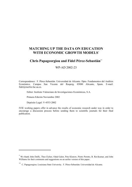
<strong>MATCHING</strong> <strong>UP</strong> <strong>THE</strong> <strong>DATA</strong> <strong>ON</strong> EDUCATI<strong>ON</strong><br />
<strong>WITH</strong> EC<strong>ON</strong>OMIC GROWTH MODELS *<br />
Chris Papageorgiou and Fidel Pérez-Sebastián **<br />
WP-AD 2002-23<br />
Correspondence: F. Pérez-Sebastián. Universidad de Alicante. Dpto. Fundamentos del Análisis<br />
Económico. Campus San Vicente del Raspeig. 03080 Alicante, Spain. E-mail:<br />
fidel@merlin.fae.ua.es.<br />
Editor: Instituto Valenciano de Investigaciones Económicas, S.A.<br />
Primera Edición Noviembre 2002<br />
Depósito Legal: V-4553-2002<br />
IVIE working papers offer in advance the results of economic research under way in order to<br />
encourage a discussion process before sending them to scientific journals for their final<br />
publication.<br />
* We thank John Duffy, Theo Eicher, Oded Galor, Pete Klenow, Pietro Peretto, B. Ravikumar, and John<br />
Williams for their comments and suggestions on an earlier version of this paper.<br />
** C. Papageorgiou: Louisiana State University. F. Pérez-Sebastián: Universidad de Alicante.
<strong>MATCHING</strong> <strong>UP</strong> <strong>THE</strong> <strong>DATA</strong> <strong>ON</strong> EDUCATI<strong>ON</strong><br />
<strong>WITH</strong> EC<strong>ON</strong>OMIC GROWTH MODELS<br />
Chris Papageorgiou and Fidel Pérez-Sebastián<br />
A B S T R A C T<br />
The growth literature has not yet established how data on education<br />
should be introduced in theories involving human capital. Early work used<br />
enrolment rates as a proxy of human capital whereas more recently it has<br />
utilized measures of average educational attainment taking advantage of new<br />
data sets. This paper examines alternative specifications of human capital that<br />
may match up with the existing data on education. First, we present a standard<br />
neoclassical two-sector growth model that adopts a human capital specification<br />
proposed in recent papers. In this model the fraction of individual's time<br />
endowment in school is viewed as an investment rate. We show that the<br />
optimally chosen educational attainment predicted by the calibrated model is<br />
very high and does not correspond to the data. Next, we consider two<br />
extensions of the basic model: (a) allow for different elasticities of substitution<br />
between skilled and unskilled labor, (b) introduce work experience. We find<br />
that neither of the two extensions are able to generate plausible predictions.<br />
Finally, we propose an alternative specification of human capital based on a law<br />
of motion of educational attainment that successfully matches up with the data.<br />
JEL Classification: O15, O41.<br />
Keywords: Educational attainment, Economic growth.<br />
2
1 Introduction<br />
Even though human capital has been established as one of the primary engines of economic growth<br />
and development, it has not yet been established how data on educational attainment should be<br />
introduced in growth models. 1 In this paper we ask the question: In the context of our theories<br />
of economic growth, what is an appropriate specification of human capital to which a measure of<br />
workers’ average years of schooling successfully corresponds? Our primary goal is to search for<br />
specifications that, within a simple calibrated growth model, can successfully produce educational<br />
attainment levels comparable to those observed in the data.<br />
We start by incorporating the human capital specification suggested by Bils and Klenow (1996)<br />
and Jones (1997, 2001), among others, in a very basic neoclassical two-sector growth model. In<br />
order to reconcile agents’ finite schooling levels with the infinite horizon model, these papers propose<br />
interpreting average years of schooling as the fraction of an individual’s time endowment allocated<br />
to accumulating skill; that is, they interpret average years of schooling as an investment rate. 2 By<br />
using the proposed interpretation of educational attainment this problem is potentially resolved. In<br />
addition, this interpretation is shown to be particularly useful in empirical tests of the relationship<br />
between income growth and human capital (see Jones (1996)).<br />
Next, we calibrate the model at steady state and compare its predictions to the data. The main<br />
finding is that the calibrated model implies an optimally chosen educational attainment level that<br />
has a lower bound of more than 30 years, whereas the data support much smaller levels (i.e. 8-14<br />
years). We interpret this finding as suggesting that the human capital technology used in the basic<br />
model is too simple.<br />
We then extend the basic specification in two different directions. First, following Mulligan and<br />
Sala-i-Martin (2000) and Temple (2001), we allow for different elasticities of substitution between<br />
skilled and unskilled labor hoping that assigning appropriate elasticities would produce a specification<br />
that works. Our calibration exercise, however, shows that educational attainment levels<br />
remain very high regardless of the degree of substitutability between raw and skilled labor. Second,<br />
we embed a version of Bils and Klenow (2000) (BK thereafter) human capital specification that<br />
includes work experience in the two-sector infinite horizon growth model, and study its equilibrium<br />
predictions. 3 We find that the later extension cannot generate plausible predictions for the average<br />
educational attainment, either.<br />
Finally, we present a simple growth model that employs an alternative specification of human<br />
1 It is widely accepted that combining educational attainment data (i.e., Barro and Lee (1993, 2000)) with labor<br />
income data obtains a reliable approximation of human capital across countries. Educational attainment data captures<br />
formal education whereas labor income data is meant to capture the remaining components of human capital such as<br />
informal education (i.e., on-the-job training and work experience, see Stokey (1988)) and health (see Schultz (1989)),<br />
for which data are either unavailable or unreliable. In a recent contribution, Mulligan and Sala-i-Martin (2000 p.<br />
216) indicate that employing only labor income data to construct human capital stocks is rather problematic, and<br />
that the use of educational attainment data is essential.<br />
2 More precisely, these papers attempt to take issue with the following potential shortcoming inherent in the infinite<br />
horizon neoclassical growth model: when individuals face an infinite horizon they invest in education every period<br />
making educational attainment grow with the economy, which is counter-factual.<br />
3 In an important contribution, BK specify a human capital production function thatisbasedonthe“Macro-<br />
Mincer” wage equation, inspired by the labor economics literature, and empirically tested by Heckman and Klenow<br />
(1997) and Temple (2001). BK present a finite-lived-agent model of schooling and economic growth that is capable of<br />
producing levels of educational attainment that comply with the data. Unlike BK and consistent with the neoclassical<br />
framework, the models considered in our paper fall under the infinite-horizon class.<br />
3
capital. The proposed specification does not include additional variables such as work experience.<br />
Instead, it provides a map between schooling investment and human capital accumulation through a<br />
law of motion of educational attainment. A calibration exercise reveals that the model is successful<br />
in predicting educational attainment levels consistent with those observed in the data.<br />
The rest of the paper is organized as follows. Section 2 investigates the steady-steady properties<br />
of a basic infinite horizon two-sector growth model following the specification used in recent papers.<br />
Section 3 incorporates a version of BK’s human capital specification in our basic model, and<br />
investigates its steady-state educational attainment predictions. Section 4 proposes an alternative<br />
specification of human capital that features a law of motion of educational attainment. Section 5<br />
concludes.<br />
2 The Basic Model<br />
Interpreting an individual’s time endowment in school as an investment rate seems, at first pass, to<br />
be appealing and worthy of further investigation. As such, the aim of this section is to investigate the<br />
implications of a standard two-sector growth model, using the human capital specification suggested<br />
in Jones (1997, 2001). Even though attention is focused on the neoclassical growth model, it is<br />
shown that the results extend to the richer in structure R&D-based models (see footnote 8).<br />
2.1 Economic environment<br />
The economy contains households and firms. Each household consists of identical infinitely-lived<br />
agents who are endowed with one unit of time and are involved in two types of activities: consumption<br />
goods production, and human capital investment. Labor and technology grow exogenously<br />
at rates n and g A , respectively. Given neoclassical assumptions, the decentralized and centralized<br />
problems obtain same equilibrium outcomes. For ease of exposition we focus on the central<br />
planner’s problem.<br />
The model economy is characterized by the following two equations. First, the aggregate production<br />
function<br />
Y (t) =K(t) 1−α [A(t) H Y (t)] α , 0 < α < 1; (1)<br />
where Y (t) is output at period t; K is the stock of physical capital; A is the exogenously growing<br />
labor-augmenting technology; H Y is skilled-labor input allocated in final output production; and<br />
(1 − α) is the share of capital stock.<br />
Second, the skilled-labor equation that determines the way by which skill is formed and embodied<br />
into labor<br />
H Y (t) =e f(l h(t)) (1 − l h (t)) L (t); (2)<br />
where l h is the fraction of each agent’s time endowment allocated to education; and L is labor size.<br />
Our choice of skilled-labor technology follows the Mincerian interpretation of human capital. 4 The<br />
4 The Mincerian interpretation of human capital is originated by Bils and Klenow (1996, 2000) and is based on<br />
what Heckman and Klenow (1997) call the “Macro-Mincer” wage equation:<br />
log W g it = β 0 + β 1 S it + υ it ;<br />
where W g it<br />
is the geometric mean wage for country i at time t; S is mean years of education; and υ is a random<br />
error. This interpretation has been adopted by many recent papers including Jones (1997, 2001) and Hall and Jones<br />
4
function f (l h (t)) simply states that productivity from education depents on time in schooling.<br />
Consistent with our analysis, we show later on that by reinterpreting l h as the fraction of an<br />
agents’ “productive life” spent in school, it becomes a positive function of the average educational<br />
attainment level S, i.e.l h = g(S). 5 Let β denote the return to schooling estimated in a Mincerian<br />
wage regression: an additional year of schooling raises a worker’ efficiency by β × 100 percent. It<br />
is then easy to show that the Mincerian coefficient is 6<br />
β = f (l h )g (S). (3)<br />
2.2 Social planner’s problem<br />
Let lower case letters indicate variables normalized by the size of labor. Also, let c denote per capita<br />
consumption. A central planner would choose the sequence {k (t) ,c(t) ,l h (t)} ∞ t=0<br />
to maximize the<br />
lifetime utility of the representative consumer subject to the feasibility constraints of the economy.<br />
The problem is stated as follows:<br />
max<br />
{k,c,l h }<br />
∞<br />
0<br />
e −ρt c(t)1−θ − 1<br />
1 − θ<br />
dt, 0 < ρ < 1, θ > 0; (4)<br />
subject to,<br />
y = k 1−α Ae f(l h) (1 − l h ) α<br />
(5)<br />
˙k = y − c − (n + δ) k (6)<br />
˙L = nL (7)<br />
Ȧ = Ag A (8)<br />
L 0 ,K 0 ,A 0<br />
given;<br />
where, ρ is the discount factor; θ is the inverse of the intertemporal elasticity of substitution;<br />
δ is the depreciation rate of capital; n and g A are the exogenously growing rates of labor and<br />
technogy, respectively; and L 0 ,K 0 ,A 0 are the initial levels of labor, physical capital and technology,<br />
respectively. Equation (6) is the standard law of motion of the stock of per capita physical capital,<br />
as well as a feasibility constraint.<br />
The first order conditions (FOCs) for the interior solution obtain the optimal share of time<br />
allocated to education as<br />
lh ∗ = 1− 1<br />
f lh<br />
∗ , if f (lh) ∗ > 1<br />
= 0, otherwise; (9)<br />
(1999), just to name a few. Empirical investigation of the effects of human capital on economic growth based on the<br />
“Macro-Mincer” earnings equation is carried out by Krueger and Lindahl (1999) and Temple (2001).<br />
5 Hereafter, we assume that educational attainment takes the form of formal schooling.<br />
6 The term e f(l h(t)) of equation (2) now takes the form e f(g(S)) ,whereS is educational attainment as measured<br />
by average years of education. The Mincerian coefficient β is the first derivative of f(g(S)) with respect to S, hence<br />
β = f (g(S))g (S) =f (l h )g (S).<br />
5
where (*) denotes steady-state values. 7 Equation (9) states that at the margin, the cost of investing<br />
one more unit of labor in education must equal its benefit, which is the increase in effective labor<br />
from additional schooling in the output sector. 8 The above equation implies that human capital<br />
investment may not occur if the returns to schooling are not sufficiently large. 9<br />
2.3 Calibrating the basic model at steady state<br />
One way to evaluate a model is to formally calibrate its parameters and compare its predictions to<br />
the data, as suggested by Klenow and Rodríguez-Clare (1997). When we introduce a human capital<br />
technology in a growth model, we aim to pin down the human capital measure that corresponds<br />
to the data. Accordingly, we examine our basic model’s steady-state predictions regarding the<br />
schooling variable, lh ∗.<br />
To start with, we need to establish a range of steady-state educational attainment values that<br />
is consistent with evidence. Barro and Lee (2000), in an updated version of their 1993 paper,<br />
present data on average educational attainment for 142 countries. They report that in year 2000,<br />
average educational attainment of the eighteen richest countries ranged from 7.2 years (Italy) to<br />
12.1 years (U.S.). In an earlier study, Psacharopoulos (1994) reported a maximum value of average<br />
educational attainment equal to 13.6 for the U.S. Given this evidence, we suggest that a reasonable<br />
steady-state educational attainment value may be between 8 and 14 years. 10<br />
Next, following Jones (2001), we impose the following explicit function that maps the population’s<br />
average years of schooling S into the investment variable l h :<br />
l h = S N ; (10)<br />
where N is the number of years of “productive life” of an individual. 11 The relationship between<br />
l h and S given by equation (10) is certainly true at steady state. Notice that the optimal schooling<br />
7 As will be shown later on, the assumption f (lh) ∗ > 1 is supported by the data. In particular, it is shown that<br />
f (lh) ∗ is equal to the return to education β, multiplied by the “productive life” of an individual N. Given that the<br />
lower bound on β in the empirical literature is 0.05, the condition f (lh) ∗ > 1obtainsifN>20. Thisiscertainly<br />
very plausible (in our calibration exercises we use N =54).<br />
8 As mentioned at the beginning of this section, our results hold for the R&D-based model as well. More specifically,<br />
in a richer model with monopolistic competition and an R&D sector, we follow Perez-Sebastian (2000) and specify<br />
a law of motion for technology, Ȧ = µA φ e f(lh) l A L λ A<br />
w ψ,whereHA<br />
= e f(lh) l<br />
A<br />
A L is the skilled-labor input<br />
employed in R&D; A w is the stock of existing technology in the world that grows at an exogenous rate g A w; µ is a<br />
parameter that determines the rate by which a new variety arrives; φ is a positive externality due to the stock of<br />
existing technology; λ is a negative externality due to duplication of effort; and ψ is a technology gap parameter. In<br />
this extended model our equation (2) becomes H J (t) =e f(lh(t)) l J (t) L (t) , where l J is the fraction of the agent’s time<br />
endowment allocated to productive activity J (∀ J = Y, A). Solving the optimal problem obtains gA ∗ = λ n as in<br />
1−φ<br />
Jones (1995). Along the balanced-growth path, the amount of time allocated to schooling and R&D is lh ∗ =1− 1<br />
f (l ∗ h)<br />
and lA ∗ 1−l<br />
=<br />
∗ h<br />
respectively, where r is the return to physical capital. The R&D-based model’s<br />
1<br />
λ g<br />
A<br />
∗ [r ∗ −n−(φ−ψ)g<br />
A]+1 ∗<br />
predictions about educational attainmentarethesameasthoseofthetwo-sectorneoclassicalgrowthmodel.<br />
9 To save space, we hereafter omit the corner solution in the expressions determining the optimal share of labor in<br />
schooling.<br />
10 Since the early 1950s, average educational attainment has been increasing in all industrial countries. For example,<br />
Barro and Lee (2000) report that in the U.S. average educational attainment in 1960 was 8.5 years,increasingto11.9<br />
in 1980, and reaching 12.1 years in 2000. Even though we assume 14 years as a sensible upper bound of educational<br />
attainment, higher values that are economically feasible do not change our results qualitatively.<br />
11 Even though in our model agents are infinitely lived, N is introduced for the purpose of calibrating the model<br />
6
decision given by equation (9) is now a function of the Mincerian returns to education, as equations<br />
(3) and (10) imply that f (l ∗ h )=βN.<br />
Finally, in order to examine whether the model’s predictions for l h and S comply with the<br />
data, we need to choose values for β and N. Regarding β, we run a sensitivity analysis employing<br />
BK’s estimates of Mincerian returns to education: β = {0.05, 0.099, 0.15}. 12 We choose the average<br />
“productive life” of individuals to be 54 years (i.e. N = 54). This value is obtained from subtracting<br />
6 years (our assumed pre-schooling period) from 60 years (our assumed retirement age). 13<br />
Table 1: Predictions of the Basic Model<br />
β N l ∗ h S ∗<br />
0.05 54 0.63 34.0<br />
0.099 54 0.81 43.9<br />
0.15 54 0.88 47.3<br />
Substituting our chosen values for β and N into equation (9), we obtain the predictions presented<br />
in Table 1. For β =0.05, the basic model predicts that average years of education S ∗ =34.0. For<br />
β =0.099, 0.15, the average years of education S ∗ reaches 43.9 and47.3 years, respectively. The<br />
predicted values of schooling are obviously too high and are far away from our acceptable range<br />
of 8 − 14 years. This finding suggests that the skilled-labor specification of the basic model is too<br />
simple and not consistent with evidence.<br />
2.4 Substitutability between skilled and unskilled labor<br />
In this section, we extend the production technology given by equation (1) by relaxing the assumption<br />
that raw and skilled labor are perfect substitutes. We then calibrate the model and once again<br />
ask whether such a specification is successful in predicting educational attainment consistent with<br />
the data. In particular, we examine a nested Constant Elasticity of Substitution (CES) aggregate<br />
output specification as follows: 14<br />
<br />
<br />
υ α/υ<br />
Y = K 1−α A zL υ u +(1− z) e f(lh) (1 − l h ) L s , −∞ < υ ≤ 1; (11)<br />
where z is what Arrow et al. (1961) refer to as the distribution parameter; L u is the number of<br />
unskilled workers who allocate zero time in schooling; L s is the number of skilled workers, who<br />
allocate a fraction of their time, l h , to schooling; and σ = 1<br />
1−υ<br />
is the elasticity of substitution<br />
between skilled and unskilled labor.<br />
and assigning values to f (l ∗ h). Furthermore, notice that equation (10) is the consequence of interpreting average<br />
years of schooling as the fraction of an individual’s time endowment allocated to accumulating skill.<br />
12 BK’s estimates of the average returns to schooling fall into the 5% −15% range, with a mean value of 9.9%. BK’s<br />
estimates are consistent with those in Psacharopoulos (1994).<br />
13 Our calculation of N is consistent with that of BK who assume N =54.5.<br />
14 Temple (2001) has empirically tested an aggregate production specification similar in spirit to our specification<br />
(11).<br />
7
In the production function given by equation (11), skilled and unskilled workers are combined<br />
into an aggregate by a CES specification. The resulting labor aggregate is then combined with the<br />
stock of physical capital by a Cobb-Douglas technology. Dividing both sides of equation (11) by<br />
the total number of workers, L = L u + L s , and denoting L u<br />
L<br />
= l gives<br />
<br />
<br />
υ α/υ<br />
y = k 1−α A zl υ +(1− z) e f(lh) (1 − l h )(1− l)<br />
. (12)<br />
The social planner’s problem can now be stated as<br />
max<br />
{k,c,l h ,l}<br />
∞<br />
0<br />
e −ρt c(t)1−θ − 1<br />
dt<br />
1 − θ<br />
subject to,<br />
<br />
<br />
<br />
y = k 1−α A zl υ +(1− z) e f(lh) υ α/υ<br />
(1 − l h )(1− l)<br />
and<br />
˙k = y − c − (n + δ) k<br />
˙L = nL<br />
Ȧ = Ag A<br />
L 0 ,K 0 ,A 0<br />
given.<br />
At steady state, the FOCs for the interior solution imply the following optimal allocation<br />
lh ∗ =1− 1<br />
f (lh ∗ (13)<br />
);<br />
l ∗ 1<br />
= 1<br />
1+ z υ−1<br />
1−z<br />
e f(l∗ h ) (1 − lh ∗ υ<br />
. (14)<br />
)<br />
1−υ<br />
Notice that equation (13) is identical to equation (9). This is easy to see by comparing production<br />
functions (12) and (5). Let x be the marginal cost of investing in education. In both cases,<br />
the marginal benefit from schooling equals x ∗ f (l h )(1 − l h ). That is, cost and benefit change<br />
proportionally when we introduce unskilled labor. Hence, the optimal value of l h does not vary.<br />
It is important to notice that lh ∗ now reflects schooling time of skilled workers. Even when we<br />
assume that a skilled worker has completed college education and possesses 16 years of schooling,<br />
the model predicts values that remain implausibly high.<br />
In addition to the aggregate specification of equation (11), we have also experimented with the<br />
specification proposed by Stokey (1996). Stokey’s aggregate production technology is consistent<br />
with the capital-skill complementarity hypothesis advanced by Griliches (1969) and supported by<br />
many researchers (see Hamermesh (1993) p. 113 and more recently Krusell et al. (2000)). Our<br />
aggregate specification now takes the form<br />
Y = A [zK υ +(1− z)L υ u] α/υ e f(l h) (1 − l h )L s + ξL u<br />
1−α<br />
; (15)<br />
where z is the distribution parameter; and ξ is the relative efficiency of unskilled labor in supplying<br />
mental effort. In the above production function, capital and unskilled workers are combined into an<br />
8
aggregate by a CES specification. The resulting aggregate measure is then combined with skilled<br />
labor and a using a Cobb-Douglas technology. The capital-skill complementarity would hold in this<br />
case if the elasticity of substitution between capital and unskilled workers is greater than unity,<br />
> 1or0< υ ≤ 1. Solving the optimization problem delivers the same optimal share<br />
of schooling as before, i.e. lh ∗ =1− 1<br />
f (lh ∗ ), suggesting that this alternative specification may not be<br />
appropriate either.<br />
We conclude that relaxing the assumption that unskilled and skilled labor are perfect substitutes<br />
does not improve the results of the basic model.<br />
σ K,Lu = 1<br />
1−υ<br />
3 The Schooling-Experience Model<br />
Following BK, this section considers a broader concept of human capital by incorporating work<br />
experience in the basic model of section 2. 15 Hereafter, we call this modified model as the “schoolingexperience<br />
model.”<br />
Equation (2) is now replaced by the following specification:<br />
H Y (t) =e f(l h(t))+ε(1−l h (t)) (1 − l h (t)) L (t) ; (16)<br />
where ε (1 − l h (t)) is an implicit function for work experience at period t.<br />
3.1 Social planner’s problem<br />
The planner’s problem is stated as<br />
subject to,<br />
max<br />
k,c,l h ,l<br />
∞<br />
0<br />
e −ρt c(t)1−θ − 1<br />
1 − θ<br />
dt<br />
<br />
y = k 1−α Ae f(l h)+ε(1−l h ) α<br />
(1 − l h )<br />
˙k = y − c − (n + δ)k<br />
˙L = nL<br />
Ȧ = Ag A<br />
L 0 ,K 0 ,A 0<br />
given.<br />
The FOCs for the interior solution obtain the optimal share of average time endowment in<br />
education as<br />
lh ∗ 1<br />
=1−<br />
f (lh ∗) − ε (1 − lh ∗ (17)<br />
).<br />
Notice that lh ∗ is now different from that in the basic model given in equation (9) — there is<br />
an additional term, ε (1 − lh ∗ ), appearing in the denominator. Equation (17) implies that in the<br />
15 In addition to work experience, BK allow schooling time to enter in agent’s utility function. This assumption<br />
is supported by Schultz (1963) who argues that an individual is happier going to school than working. They also<br />
correct for quality of education by including teacher human capital in the human capital specification. Both terms<br />
raise the marginal benefit from education, and their introduction into our specification would generate larger values<br />
of S ∗ . This is indeed the opposite effect of what our model needs to generate sensible results.<br />
9
experience-schooling model, time in formal schooling is reduced because work experience presents<br />
an alternative engine of skill formation. Put differently, agents who are now able to enhace their<br />
skill level from schooling as well as working, choose an optimal time allocation to formal education<br />
that is lower than the one in the basic model.<br />
Table 2: Predictions of the Schooling-Experience Model<br />
γ 1 =0.0512, γ 2 = −0.00071<br />
β N l ∗ h S ∗<br />
0.05 54 0.50 27.0<br />
0.099 54 0.73 39.4<br />
0.15 54 0.83 45.0<br />
γ 1 =0.0846, γ 2 = −0.00108<br />
β N l ∗ h S ∗<br />
0.05 54 0.42 22.9<br />
0.099 54 0.66 35.5<br />
0.15 54 0.79 42.8<br />
γ 1 =0.0934, γ 2 = −0.00110<br />
β N l ∗ h S ∗<br />
0.05 54 0.38 20.6<br />
0.099 54 0.63 33.9<br />
0.15 54 0.78 42.0<br />
3.2 Calibrating the schooling-experience model at steady state<br />
For the calibration exercise, we need to assign values to ε (1 − l h ). To do this, we employ estimates<br />
of Mincerian returns on experience, which are in general based on the following quadratic equation:<br />
ε(p(E)) = γ 1 E + γ 2 E 2 ; (18)<br />
where E is the worker’s years of experience; and p is an explicit function that maps E into the<br />
investment variable (1 − l h ). This quadratic form implies a Mincerian return on experience equal<br />
to ε (p(E)) = ε (1 − l h ) p (E) =γ 1 +2γ 2 E. Hence,<br />
ε (1 − l h )= γ 1 +2γ 2 E<br />
p . (19)<br />
(E)<br />
Consistent with equation (10), and for the purpose of this calibration exercise, we assume that<br />
(1 − l h )=p(E) = E N . (20)<br />
In equation (20), the term (1 − l h ) is interpreted as the fraction of the individuals’ productive life<br />
in the work-place accumulating experience. Finally, expressions (19) and (20) deliver<br />
ε (1 − l ∗ h)=N [γ 1 +2γ 2 (1 − l ∗ h)N] . (21)<br />
Values for γ 1 =0.0512 and γ 2 = −0.00071 are obtained from BK, and they reflect the average<br />
estimates of the Mincerian returns to experience across 52 countries. 16 Recalling that f (l ∗ h )=βN,<br />
16 For more discussion on these estimates see BK (p.1167 and appendix B).<br />
10
we can now recover lh ∗ using equations (17) and (21).17 The predicted values of average years in<br />
schooling are given in Table 2. For β =0.05 the value of S ∗ is 27.0. As expected this value is lower<br />
than that in the basic model (see Table 1), but still much higher than our acceptable range of 8−14<br />
years. For β equal to 0.099 and 0.15, the implied values of S ∗ are implaussible.<br />
The above numbers are certainly sensitive to the choice of γ 1 and γ 2 . Recall from equation<br />
(17) that the optimal value of lh ∗ and therefore S∗ decrease with the return to experience. As a<br />
robustness check of our results, we take the average values for the 10 countries in the BK sample<br />
with largest γ 1 ; this obtains γ 1 =0.0846 and γ 2 = −0.00108. As we see in Table 2, the minimum<br />
educational attainment is still large, 22.9 years. If we go even further and calculate the average for<br />
the 5 countries with the largest γ 1 ,wegetγ 1 =0.0934 and γ 2 = −0.00110. Table 2 reveals that<br />
the optimal number of years of education in this case is 20.6, again implausibly high. 18<br />
A parameter to which the predictions of both the basic and schooling-experience models are<br />
sensitive is the individual’s productive life, N. It is easy to show that in both models, average years<br />
of schooling S ∗ declines with N. In the basic model, S ∗ = 14 (our upper bound) only when N =34,<br />
whereas in the most favorable case of the schooling-experience model, S ∗ =14whenN = 47. Both<br />
values of N are lower than our assumed parameter N =54. 19<br />
Unlike the basic model, the schooling-experience model can raise the marginal cost of education<br />
investment through the experience parameter. This reduces the optimal amount of schooling time<br />
and consequently the steady-state level of educational attainment. The predicted values, however,<br />
remain implausibly high. We conclude that even though the introduction of a working-experience<br />
term in the human capital specification improves the educational attainment predictions of the<br />
model, it is not sufficient to make these predictions plausible.<br />
4 An Alternative Specification of Skilled-Labor<br />
In this section, we offer an alternative skilled-labor specification that delivers educational attainment<br />
levels that are consistent with those in the data. An attractive feature of the proposed<br />
specification is that it does not include additional variables such as work experience, which makes<br />
it easy to incorporate into existing growth models.<br />
Final output production is once again given by equation (1). Human capital per capita is now<br />
expressed as<br />
h (t) =e f(S(t)) . (22)<br />
The derivative f (S(t)) represents the returns to schooling estimated in a Mincerian wage regression.<br />
As in the basic model, we assume that at period t agent i invests a fraction, l h (t, i), of his time in<br />
education and that population grows at rate n. Years of schooling accumulate through educational<br />
17 Combining equations (17) and (21) results in a quadratic equation. It turns out that for each of three quadratic<br />
equations associated with the values of β, one of two real roots is economically infeasible (greater than unity). We<br />
report the feasible values of l ∗ h, and the corresponding values of S ∗ . Once again, S ∗ is recovered using equation (10).<br />
18 Avalueofγ 1 equal to 0.0934 represents the average in the BK sample plus 1.96 standard deviations. It is also<br />
important to notice that, in the BK sample, larger values of γ 1 are generally associated with lower values of γ 2 ,with<br />
a correlation coefficient between the two parameters of −0.61.<br />
19 As mentioned previously, BK use N =54.5 whichisveryclosetoourchosenparameter. They calculate N by<br />
taking the average life expectancy 60.5 (see Barro and Lee (1993)) minus 6 years, the typical pre-schooling period.<br />
11
investment. Average educational attainment equals<br />
S(t) = 1 t <br />
L(j)<br />
l h (j, i) di<br />
L(t)<br />
0<br />
0<br />
dj. (23)<br />
Differentiating expression (23) with respect to t delivers the following law of motion of the average<br />
educational attainment, S:<br />
Ṡ(t) =l e h(t) − nS(t); (24)<br />
where l e h (t) =[1/L(t)] [ L(t)<br />
0 l h (t, i) di] is the economy-wide fraction of time allocated to acquiring<br />
skills. This law of motion is equivalent to the standard motion of physical capital. Equation (24)<br />
says that, at the aggregate, workers’ average educational attainment increases with the fraction of<br />
time that agents invest in schooling, but (exogenously) declines with the increase of population.<br />
The new human capital formulation introduces an externality. Equations (1), (22) and (24)<br />
imply that labor productivity depends on the average educational attainment in the economy. A<br />
worker’s investment in education, therefore, has positive external effects on other workers productivity.<br />
For simplicity, we keep focusing on the centralized solution.<br />
4.1 Social planner’s problem<br />
The social planner’s problem is the following:<br />
max<br />
{k,c,l h ,S}<br />
∞<br />
0<br />
e −ρt c(t)1−θ − 1<br />
1 − θ<br />
dt<br />
subject to,<br />
<br />
y = k 1−α Ae f(S) (1 − lh)<br />
e α<br />
˙k = y − c − (n + δ) k<br />
Ṡ = lh e − nS<br />
˙L = nL<br />
Ȧ = Ag A<br />
L 0 ,K 0 ,A 0 ,S 0<br />
given.<br />
We construct the Hamiltonian, and get the FOCs for the interior solution. After some algebra<br />
we show that the Euler equation that characterizes the optimal allocation of labor to human capital<br />
investment is<br />
ẏ<br />
f (S)(1− lh)+<br />
e y +<br />
˙l h<br />
e <br />
1 − lh<br />
e = r; (25)<br />
where r is the interest rate that is given by<br />
r =(1− α) y k − δ = ρ + θ ċ + n. (26)<br />
c<br />
Equation (26) is the standard Euler condition for consumption. Expression (25) can be interpreted<br />
as an arbitrage condition. The LHS of equation (25) is the returns to sacrificing one unit of output<br />
12
for acquiring schooling. The first term represents the dividend from the increase in effective labor.<br />
The term in brackets represents the capital gain/loss, which is equal to the percentage change in<br />
the price of education — notice that the shadow price of having additional units of education equals<br />
α y<br />
the marginal productivity of labor in output production,<br />
1−l h<br />
. The RHS of equation (25) captures<br />
the opportunity cost of schooling investment, given by the interest rate. In equilibrium, both sides<br />
must be equalized.<br />
Let g j be the steady-state growth rate of variable j. Along the balanced growth path g y = g c ,<br />
and ˙l h e = 0. Euler equations (25) and (26) then imply that the optimal share of labor in schooling<br />
is<br />
<br />
n + ρ +(θ − 1)<br />
lh e∗<br />
gy<br />
=1−<br />
f (S ∗ . (27)<br />
)<br />
The optimal education investment depends directly on its current return f (S ∗ ) and the future<br />
benefits, which grow with g y , of applying the acquired knowledge. As expected, the optimal<br />
education investment declines with the preference parameters ρ and θ, and the population growth<br />
rate n.<br />
4.2 Calibrating the alternative model at steady state<br />
We choose the standard values g y =0.02 , ρ =0.04 , n =0.016 , and θ ∈ [1, 2] from the existing<br />
literature. 20 We then use equation (27) to generate values for lh<br />
e∗ and S∗ . Table 3 presents estimates<br />
of lh e∗ and S∗ for different values of θ = {1, 2} and β = {0.05, 0.068, 0.099, 0.15}.<br />
Table 3: Predictions of proposed model without an explicit function for f (S)<br />
β θ lh<br />
e∗ S ∗<br />
0.05 1 − −<br />
0.068 1 0.18 11.0<br />
0.099 1 0.43 27.1<br />
0.15 1 0.63 39.2<br />
β θ l e∗<br />
h S ∗<br />
0.05 2 − −<br />
0.068 2 − −<br />
0.099 2 0.23 14.5<br />
0.15 2 0.49 30.0<br />
We find that for β =0.068 (the OECD average in Psacharopoulos (1994)) and θ =1, the<br />
calibrated share of labor in schooling is lh<br />
e∗ =0.18, and the resulting mean years of schooling is<br />
11.0. In the case where β =0.097 and θ = 2, the model predicts that lh e∗ =0.23, and S∗ =14.5<br />
which is close to our upper value of 14 years and the value reported by Psacharopoulos (1994) for<br />
the U.S. (SU.S. ∗ =13.6 years). These estimates are more consistent with the data.<br />
So far, we have taken β as exogenous to generate predictions. But the Mincerian return to<br />
schooling is actually a function of S. A tougher test of the proposed model is to give an explicit<br />
form to β(S) and examine whether the predictions still comply with the data. Following BK, we<br />
assume that β = ηϕSt ϕ−1 ,where β > 0, and 0 < ϕ ≤ 1, and consider three pairs for η and ϕ,<br />
20 We set the per capita output growth rate g y to 2% which is the approximate post-war per capita output growth<br />
rate for the U.S. We also set the growth rate of population n to match the average labor force growth rate in the U.S.<br />
during the period 1950-1980. A range of estimates of the inverse of the intertemporal elasticity of substitution θ are<br />
taken from Hall (1988), Attanasio and Weber (1993), and a very valuable recent contribution by Guvenen (2001).<br />
13
{0.76, 0.42}, {0.25, 0.72}, and{0.099, 1}. 21 We then exploit an equilibrium relationship between<br />
lh<br />
e∗ and S∗ obtained by the model. In particular, because at steady state lh e remains constant, the<br />
motion equation (24) implies that so does S ∗ — otherwise g S can not be a constant — and therefore<br />
S ∗ = le∗ h<br />
n . (28)<br />
Equation (27) becomes<br />
l e∗<br />
h =1−<br />
⎡<br />
⎤<br />
⎢<br />
⎣ n + ρ +(θ − 1) g y ⎥<br />
l<br />
e∗ ϕ−1 ⎦ . (29)<br />
ηϕ hn<br />
It is easy to show that equation (29) has a unique root but does not have an analytic solution when<br />
0 < ϕ < 1; we therefore use numerical approximation methods to obtain solutions.<br />
Table 4: Predictions of proposed model with f (S) =ηϕS ϕ−1<br />
η ϕ θ l ∗ h S ∗<br />
0.76 0.42 1 0.21 13.3<br />
0.25 0.72 1 0.30 18.5<br />
0.099 1 1 0.43 27.1<br />
η ϕ θ l ∗ h S ∗<br />
0.76 0.42 2 0.15 9.1<br />
0.25 0.72 2 0.17 10.9<br />
0.099 1 2 0.23 14.5<br />
The estimates of this calibration exercise are presented in Table 4. We find that for the value<br />
of θ = 2 all three pairs of {η, ϕ} obtain plausible values for l ∗ h and S∗ . 22 The triplet {η =0.76, ϕ =<br />
0.42, θ =1} also delivers plausible values. 23<br />
The main finding here is that our calibrated model is able to deliver levels of educational<br />
attainment consistent to those in the data. In other words, for values of θ ∈ [1, 2] there is a value<br />
of f (S) (or a pair of η and ϕ) that provides educational attainment levels that are consistent with<br />
those in the data (i.e. S ∗ ∈ [8, 14]). This is the result of the dynamic structure of the proposed<br />
human capital accumulation technology that is able to reduce sufficiently the overall returns to<br />
education.<br />
5 Conclusion<br />
This paper has searched for specifications of human capital that can match existing data on educational<br />
attainment with economic growth models. We have first examined a simple two-sector<br />
21 BK regress country estimates of Mincerian returns on country schooling levels in Psacharopoulos (1994) 56-<br />
country sample. They obtain the estimate 1 − ϕ =0.58 which implies diminishing Mincerian returns to schooling<br />
across nations. They also consider two other values; 1 − ϕ =0.28 (their point estimate minus two standard errors)<br />
and 1 − ϕ = 0 (no diminishing returns). For each value of ϕ they set the value η so that the mean of β = ηϕS ϕ−1<br />
equals the mean Mincerian return across Psacharopoulos’ sample of 56 countries, which is 0.099.<br />
22 Notice that the last row of table 4 is identical to the next to last row of table 3. This is because when {η, φ} =<br />
{0.099, 1} the two specifications are identical.<br />
23 A sensitivity analysis shows that our results are robust to changes in the parameters g y , ρ and n.<br />
14
growth model with a human capital specification found in recent papers. Calibrating the basic<br />
model reveals several caveats associated with this specification, and casts doubts in its use in theoretical<br />
and empirical work. In particular, the model predicts that the optimally chosen educational<br />
attainment is between 34 and 47 years, whereas the actual levels observed in the data are between<br />
8 and 14 years. Two alternative models that employed a CES specification to aggregate skilled and<br />
unskilled labor have also been examined without any success.<br />
We have then followed Bils and Klenow (2000) by incorporating work experience in addition to<br />
schooling in the basic model. Our main result is that even though incorporating experience in the<br />
human capital specification improves the educational attainment predictions of the model, it is not<br />
sufficient to make these predictions plausible.<br />
Finally, we have presented an alternative specification of human capital that incorporates an<br />
explicit law of motion of the mean years of education. An important feature of the proposed<br />
specification is that it does not include additional variables such as work experience, which makes it<br />
easy to incorporate into existing theoretical growth models and easy to adopt in growth accounting<br />
exercises. The proposed model is a standard infinite-horizon neoclassical growth model that uses<br />
parameters found in the literature. Simple calibration exercises of the model at steady state reveal<br />
that the proposed specification of human capital is successful in replicating the observed data on<br />
educational attainment.<br />
It is obvious that our results are conditional on the parameter values chosen to carry out the<br />
calibration exercises. A parameter to which the predictions of the basic and schooling-experience<br />
models are especially sensitive, is the individual’s “productive life,” N. Our sensitivity analysis on<br />
N reveals an important weakness of the human capital specification employed in recent models.<br />
These models take the market return to human capital investment as contemporaneous and immediate,<br />
whereas in practice the return to schooling is accrued over an individual’s lifetime. This<br />
leads to overstating the return to schooling, and predicting too high educational attainment levels.<br />
Introducing experience, and decreasing the individual’s “productive life” are necessary adjustments<br />
to reduce the return to schooling in the basic model.<br />
In contrast, our proposed human capital specification does not require experience, or lower<br />
“productive life” to obtain desirable predictions. This is because when human capital accumulates,<br />
preference parameters such as ρ and θ that determine intertemporal decisons, discount the return<br />
to schooling sufficiently to deliver sensible values of the average educational attainment. Another<br />
attractive feature of our human capital specification is that it may be used for off-steady-state<br />
analysis as well. Further work with our proposed specification revealed that outside the balanced<br />
growth path, enrollment rates and the average educational attainment are negatively correlated,<br />
which is the relationship that dominates the data (see Pritchett (1997) pp. 27-30).<br />
The conclusions of the paper for future research are twofold. First, incorporating the proposed<br />
human capital specification into an R&D-based model and examining the transitional dynamic<br />
properties of the model is a promising next step. Second, using the reduced form equation implied<br />
by our alternative specification, one can reexamine accounting exercises such as those in Klenow<br />
and Rodríguez-Clare (1997a), Hall and Jones (1999) and Temple (2001).<br />
15
References<br />
Arrow, K., Chenery, H., Minhas, B. and Solow, R., “Capital—Labor Substitution and Economic<br />
Efficiency,” Review of Economics and Statistics, 43:225—250, 1961.<br />
Attanasio, O. and Weber, G., “Consumption, the Interest Rate and Aggregation,” Review of<br />
Economic Studies, 60:631—649, 1993.<br />
Barro, R. and Lee, J.,“International Comparisons of Educational Attainment,” Journal of Monetary<br />
Economics, 32:363—394, 1993.<br />
Barro, R. and Lee, J., “International Data on Educational Attainment: Updates and Implications,”<br />
CID working paper#42, 2000.<br />
Bils, M. and Klenow, P., “Does Schooling Cause Growth or the Other Way Around?” working<br />
paper, University of Rochester, 1996.<br />
Bils, M. and Klenow, P., “Does Schooling Cause Growth?” American Economic Review, 90:1160—<br />
1183, 2000.<br />
Griliches, Z, “Capital—Skill Complementarity,” Review of Economics and Statistics, 51:465—468,<br />
1969.<br />
Guvenen, M.F., “Mismeasurement of the Elasticity of Intertemporal Substitution: The Role of<br />
Limited Stock Market Participation,” working paper, Carnegie Mellon University, 2001.<br />
Hall, R., “ Intertemporal Substitution in Consumption,” Journal of Political Economy, 96:339—<br />
357, 1988.<br />
Hall, R. and Jones, C., “Fundamental Determinants of Output Per Worker Across Countries,”<br />
Quarterly Journal of Economics, 114:83—116, 1999.<br />
Hamermesh, D.S., Labor Demand, 2nd Ed., Princeton: Princeton University Press, 1993.<br />
Heckman, J. and Klenow, P., “Human Capital Policy,” working paper, University of Chicago,<br />
1997.<br />
Jones, C.I., “R&D—Based Models of Economic Growth,” Journal of Political Economy, 103:759—<br />
784, 1995.<br />
Jones, C.I., “Human Capital, Ideas, and Economic Growth,” working paper, Stanford University,<br />
1996.<br />
Jones, C.I., “Convergence Revisited,” Journal of Economic Growth, 2:131—153, 1997.<br />
Jones, C.I., “Sources of U.S. Economic Growth in a World of Ideas,” American Economic Review,<br />
forthcoming, 2001.<br />
Klenow, P. and Rodríguez—Clare, A., “Economic Growth: A Review Essay,” Journal of Monetary<br />
Economics, 40:597—617, 1997.<br />
Krueger, A.B. and Lindahl, M., “Education for Growth in Sweden and the World,” NBER working<br />
paper#7190, 1999.<br />
Krusell, P., L.E. Ohanian, J—V. Ríos—Rull and Violante G.L., “Capital—Skill Complementarity<br />
and Inequality: A Macroeconomic Analysis,” Econometrica, 68:1029—1053, 2000.<br />
Mulligan C.B., and Sala-i-Martin, X., “Measuring Aggregate Human Capital,” Journal of Economic<br />
Growth, 5:215-252, 2000.<br />
Perez-Sebastian, F., “Transitional Dynamics in an R&D—Based Growth Model with Imitation:<br />
Comparing its Predictions to the Data,” Journal of Monetary Economics, 45:37—61, 2000.<br />
16
Pritchett, L., “Where Has All the Education Gone?” World Bank working paper#1581, 1997.<br />
Psacharopoulos, G., “Returns to Investment in Education: A Global Update,” World Development,<br />
22:1325—1343, 1994.<br />
Schultz, T.P., The Economic Value of Education, Columbia University Press, 1963.<br />
Schultz, T.P., “Returns to Women Education,” Population, Health, and Nutrition Department,<br />
World Bank working Paper#89/001, 1989.<br />
Stokey, N.L., “Learning by Doing and the Introduction of New Goods,” Journal of Political<br />
Economy, 96:701—717, 1988.<br />
Stokey, N.L., “Free Trade, Factor Returns, and Factor Accumulation,” Journal of Economic<br />
Growth, 1:421—447, 1996.<br />
Temple, J.R.W., “Generalizations That Aren’t? Evidence on Education and Growth,” European<br />
Economic Review, 45:905—918, 2001.<br />
17


