MATCHING UP THE DATA ON EDUCATION WITH ... - Ivie

decision given by equation (9) is now a function of the Mincerian returns to education, as equations
(3) and (10) imply that f (l ∗ h )=βN.
Finally, in order to examine whether the model’s predictions for l h and S comply with the
data, we need to choose values for β and N. Regarding β, we run a sensitivity analysis employing
BK’s estimates of Mincerian returns to education: β = {0.05, 0.099, 0.15}. 12 We choose the average
“productive life” of individuals to be 54 years (i.e. N = 54). This value is obtained from subtracting
6 years (our assumed pre-schooling period) from 60 years (our assumed retirement age). 13
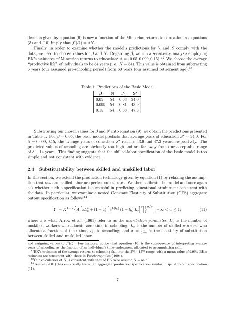
Table 1: Predictions of the Basic Model
β N l ∗ h S ∗
0.05 54 0.63 34.0
0.099 54 0.81 43.9
0.15 54 0.88 47.3
Substituting our chosen values for β and N into equation (9), we obtain the predictions presented
in Table 1. For β =0.05, the basic model predicts that average years of education S ∗ =34.0. For
β =0.099, 0.15, the average years of education S ∗ reaches 43.9 and47.3 years, respectively. The
predicted values of schooling are obviously too high and are far away from our acceptable range
of 8 − 14 years. This finding suggests that the skilled-labor specification of the basic model is too
simple and not consistent with evidence.
2.4 Substitutability between skilled and unskilled labor
In this section, we extend the production technology given by equation (1) by relaxing the assumption
that raw and skilled labor are perfect substitutes. We then calibrate the model and once again
ask whether such a specification is successful in predicting educational attainment consistent with
the data. In particular, we examine a nested Constant Elasticity of Substitution (CES) aggregate
output specification as follows: 14
υ α/υ
Y = K 1−α A zL υ u +(1− z) e f(lh) (1 − l h ) L s , −∞ < υ ≤ 1; (11)
where z is what Arrow et al. (1961) refer to as the distribution parameter; L u is the number of
unskilled workers who allocate zero time in schooling; L s is the number of skilled workers, who
allocate a fraction of their time, l h , to schooling; and σ = 1
1−υ
is the elasticity of substitution
between skilled and unskilled labor.
and assigning values to f (l ∗ h). Furthermore, notice that equation (10) is the consequence of interpreting average
years of schooling as the fraction of an individual’s time endowment allocated to accumulating skill.
12 BK’s estimates of the average returns to schooling fall into the 5% −15% range, with a mean value of 9.9%. BK’s
estimates are consistent with those in Psacharopoulos (1994).
13 Our calculation of N is consistent with that of BK who assume N =54.5.
14 Temple (2001) has empirically tested an aggregate production specification similar in spirit to our specification
(11).
7