Ein Beispiel zum Neville-Schema

Ein Beispiel zum Neville-Schema
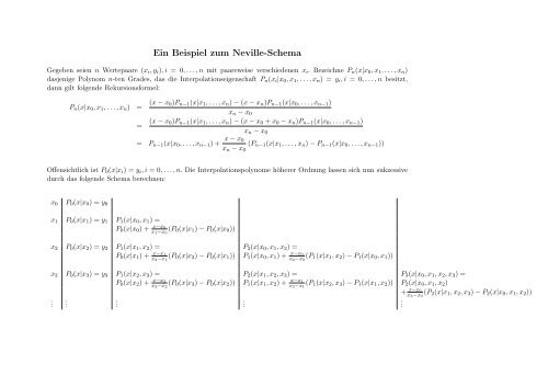
Gegeben seien n Wertepaare (x i , y i ), i = 0, . . .,n mit paareweise verschiedenen x i . Bezeichne P n (x|x 0 , x 1 , . . .,x n )
dasjenige Polynom n-ten Grades, das die Interpolationseigenschaft P n (x i |x 0 , x 1 , . . .,x n ) = y i , i = 0, . . .,n besitzt,
dann gilt folgende Rekursionsformel:
P n (x|x 0 , x 1 , . . .,x n ) = (x − x 0)P n−1 (x|x 1 , . . .,x n ) − (x − x n )P n−1 (x|x 0 , . . .,x n−1 )
x n − x 0
= (x − x 0)P n−1 (x|x 1 , . . .,x n ) − (x − x 0 + x 0 − x n )P n−1 (x|x 0 , . . .,x n−1 )
x n − x 0
= P n−1 (x|x 0 , . . .,x n−1 ) + x − x 0
x n − x 0
(P n−1 (x|x 1 , . . .,x n ) − P n−1 (x|x 0 , . . .,x n−1 ))
Offensichtlich ist P 0 (x|x i ) = y i , i = 0, . . .,n. Die Interpolationspolynome höherer Ordnung lassen sich nun sukzessive
durch das folgende Schema berechnen:
x 0 P 0 (x|x 0 ) = y 0
x 1 P 0 (x|x 1 ) = y 1 P 1 (x|x 0 , x 1 ) =
P 0 (x|x 0 ) + x−x 0
x 1 −x 0
(P 0 (x|x 1 ) − P 0 (x|x 0 ))
x 2 P 0 (x|x 2 ) = y 2 P 1 (x|x 1 , x 2 ) = P 2 (x|x 0 , x 1 , x 2 ) =
P 0 (x|x 1 ) + x−x 1
x 2 −x 1
(P 0 (x|x 2 ) − P 0 (x|x 1 )) P 1 (x|x 0 , x 1 ) + x−x 0
x 2 −x 0
(P 1 (x|x 1 , x 2 ) − P 1 (x|x 0 , x 1 ))
x 3 P 0 (x|x 3 ) = y 3 P 1 (x|x 2 , x 3 ) = P 2 (x|x 1 , x 2 , x 3 ) = P 3 (x|x 0 , x 1 , x 2 , x 3 ) =
P 0 (x|x 2 ) + x−x 2
x 3 −x 2
(P 0 (x|x 3 ) − P 0 (x|x 2 )) P 1 (x|x 1 , x 2 ) + x−x 1
x 3 −x 1
(P 1 (x|x 2 , x 3 ) − P 1 (x|x 1 , x 2 )) P 2 (x|x 0 , x 1 , x 2 )
+ x−x 0
x 3 −x 0
(P 2 (x|x 1 , x 2 , x 3 ) − P 2 (x|x 0 , x 1 , x 2 ))
.
.
.
.
.

Beispiel:
1 1
2 -1 1 + (x − 1)(−1 − 1)
= 1 − 2(x − 1) = 3 − 2x
3 2 −1 + (x − 2)(2 − (−1)) 1 − 2(x − 1) + x−1
2
(5x − 10)
= −1 + 3(x − 2) = 3x − 7 = 1 − 2(x − 1) + 5 2
(x − 1)(x − 2)
4 -2 2 + (x − 3)(−2 − 2) −1 + 3(x − 2) + x−2
2 (21 − 7x) 1 − 2(x − 1) + 5 x−1
x−2
2
(x − 1)(x − 2) +
3
(−2 + 2(x − 1) + 3(x − 2) −
2
(12x − 26))
= 2−4(x − 3) = 14 − 4x = −1 + 3(x − 2)− 7 2 (x − 2)(x − 3) = 1 − 2(x − 1) + 5 2
(x − 1)(x − 2) − (x − 1)(x − 2)12x−36
6
= 1 − 2(x − 1) + 5 2
(x − 1)(x − 2)−2(x − 1)(x − 2)(x − 3)
Welche der verschiedenen, hier benutzen Darstellungen des Polynoms man nimmt ist egal, man wird sich immer die
für den jeweiligen Zweck geeignete heraussuchen. In der allgemeinen Form enthält das Neville-Schema auch die (fett
gedruckten) Koeffizienten des Newton-Polynoms, also das Newton-Schema - hier mal zum Vergleich.
x y
1 1
1 2 -1 -2 -2
5
2 1 3 2 3 3 5
2
3 2 1 4 -2 -4 -4 -7 − 7 2
-6 -2
Benötigt man aber lediglich den Wert des Interpolationspolynoms an einer Stelle, dann kann man gleich mit diesem
x rechnen.
Beispiel: x = 1 2
1 1
2 -1 1 + ( 1 2
− 1)(−1 − 1) = 2
3 2 −1 + ( 1 2 − 2)(2 − (−1)) = −11 2 = −5, 5 2 + 1 2 −1
2 (−11 2 − 2) = 31 8
= 3, 875
4 -2 2 + ( 1 2 − 3)(−2 − 2) = 12 −11 2 + 1 2 −2
2 (12 + 11 2 ) = −149 8 = −18, 625 31
8 + 1 2 −1
3 (−149 8 − 31 8 ) = 183
24
= 7, 625