PROBLEMS OF GEOCOSMOS
PROBLEMS OF GEOCOSMOS
PROBLEMS OF GEOCOSMOS

Create successful ePaper yourself
Turn your PDF publications into a flip-book with our unique Google optimized e-Paper software.
Saint-Petersburg State University<br />
Proceedings of the 7th International Conference<br />
<strong>PROBLEMS</strong> <strong>OF</strong> <strong>GEOCOSMOS</strong><br />
St. Petersburg, Petrodvorets<br />
May 26-30, 2008<br />
Editors: V.N. Troyan, M. Hayakawa, V.S. Semenov<br />
Saint-Petersburg<br />
2008
Editors: V.N. Troyan, M. Hayakawa, V.S. Semenov. Proceedings of the 7th International<br />
Conference “Problems of Geocosmos”. – SPb., 2008 – 505 p.<br />
ISBN 978-5-9651-0303-4<br />
Copyright @ 2008 All rights<br />
reserved by V.A. Fock Institute of<br />
Physics, Physical Faculty,<br />
Saint-Petersburg State University
Proc. of the 7th Intern. Conf. "Problems of Geocosmos" (St. Petersburg, Russia, 26-30 May 2008): Contents<br />
C O N T E N T S<br />
SOLAR-TERRESTRIAL PHYSICS<br />
Amerstorfer, U.V., H.V. Erkaev, and H.K. Biernat: KELVIN-HELMHOLTZ INSTABILITY IN<br />
FINITE LARMOR RADIUS MHD AND CONSEQUENCES AT VENUS . . . . . . . . . . . . . . . .<br />
Artamonova, I.V., and S.V. Veretenenko: BARIC SYSTEM DYNAMICS DURING FORBUSH<br />
DECREASES <strong>OF</strong> GALACTIC COSMIC RAYS . . . . . . . . . . . . . . . . . . . . . . . . . . . . . . . . . . . . .<br />
Artemyev, A.V., L.M. Zelenyi, H.V. Malova, and V.Y. Popov: INSTABILITY <strong>OF</strong> THIN<br />
CURRENT SHEET . . . . . . . . . . . . . . . . . . . . . . . . . . . . . . . . . . . . . . . . . . . . . . . . . . . . . . . . . . . .<br />
Avakyan, S.V., and N.A. Voronin: TRIGGER MECHANISM <strong>OF</strong> SOLAR-ATMOSPHERIC<br />
RELATIONSHIP AND THE CONTRIBUTION <strong>OF</strong> THE ANTHROPOGENIC IMPACT . . . .<br />
Badin, V.I.: MAGNETOMETRIC SPECTRA <strong>OF</strong> AURORAL CURRENTS COMPARED WITH<br />
THE DOPPLER RADAR MEASUREMENTS . . . . . . . . . . . . . . . . . . . . . . . . . . . . . . . . . . .<br />
Baishev, D.G., E.S. Barkova, S.N. Samsonov, and K. Yumoto: SURGE-LIKE AURORAL<br />
STRUCTURES AND QUASI-PERIODIC PRECIPITATIONS <strong>OF</strong> ENERGETIC<br />
PARTICLES IN THE MORNING SECTOR: A CASE STUDY . . . . . . . . . . . . . . . . . . . . . . .<br />
Benevolenskaya, E.E.: NEW RESULTS <strong>OF</strong> SOLAR ACTIVITY AND MAGNETIC FIELD ON<br />
THE SUN (REVIEW) . . . . . . . . . . . . . . . . . . . . . . . . . . . . . . . . . . . . . . . . . . . . . . . . . . . . .<br />
Cherneva, N.V., G.I. Druzhin, and A.N. Melnikov: DIRECTION-FINDING <strong>OF</strong> A RARE<br />
PHENOMENON <strong>OF</strong> A THUNDERSTORM OVER KAMCHATKA ON THE<br />
REGISTRATION DATA <strong>OF</strong> VLF RADIATION . . . . . . . . . . . . . . . . . . . . . . . . . . . . . . . . . . . .<br />
Chugunova, O., V. Pilipenko, G. Zastenker, and N. Shevyrev: MAGNETOSHEATH<br />
TURBULENCE AND MAGNETOSPHERIC PC3 PULSATIONS . . . . . . . . . . . . . . . . . . . . . .<br />
Denisenko, V.V., A.V. Kitaev, and H.K. Biernat: TWO DIMENSIONAL MODEL <strong>OF</strong> MAGNETIC<br />
FIELD TRANSFER THROUGH THE MAGNETOTAIL DUE TO PLASMA FLOW IN THE<br />
PLASMA SHEET . . . . . . . . . . . . . . . . . . . . . . . . . . . . . . . . . . . . . . . . . . . . . . . . . . . . . . . . . . . . .<br />
Dergachev, V.A.: SECULAR AND LARGE-SCALE CHANGES IN SOLAR ACTIVITY,<br />
COSMOGENIC ISOTOPES AND CLIMATE CHANGES . . . . . . . . . . . . . . . . . . . . . . . . . . . . .<br />
Divin, A.V., V.S. Semenov, and D.B. Korovinskiy: STRUCTURE <strong>OF</strong> THE ELECTRON<br />
DIFFUSION REGION <strong>OF</strong> THE RECONNECTION PROCESS . . . . . . . . . . . . . . . . . . . . . . . . .<br />
Doronina, E.N., and A.A. Namgaladze: THE INFLUENCE <strong>OF</strong> NEUTRAL GAS HEATING AND<br />
COOLING ON THE DAY-TIME EQUATORIAL NEUTRAL DENSITY MINIMUM<br />
FORMATION . . . . . . . . . . . . . . . . . . . . . . . . . . . . . . . . . . . . . . . . . . . . . . . . . . . . . . . . . . . . . . . .<br />
Erkaev, N.V., V.S. Semenov, and H.K. Biernat: LOW FREQUENCY CURRENT SHEET<br />
OSCILLATIONS RELATED TO MAGNETIC FIELD GRADIENTS . . . . . . . . . . . . . . . . . . . .<br />
i<br />
1<br />
7<br />
12<br />
18<br />
24<br />
29<br />
34<br />
42<br />
46<br />
52<br />
57<br />
63<br />
70<br />
74
Proc. of the 7th Intern. Conf. "Problems of Geocosmos" (St. Petersburg, Russia, 26-30 May 2008): Contents<br />
Grib, S.A., and V.B. Belakhovsky: ON THE INFLUENCE <strong>OF</strong> SECONADARY RAREFACTION<br />
WAVE ON THE GEOMAGNETIC FIELD . . . . . . . . . . . . . . . . . . . . . . . . . . . . . . . . . . . . . . . . .<br />
Gubchenko, V.M.: ON A NEW PARAMETER <strong>OF</strong> SPACE WEATHER AND TOPOLOGY <strong>OF</strong><br />
THE EARTH’S MAGNETOSPHERE BASED ON THE FORM FACTOR <strong>OF</strong> THE<br />
INCOMING SOLAR-WIND PARTICLE-VELOCITY DISTRIBUTION FUNCTION . . . . . . .<br />
Guglielmi, A.V., B.I. Klain, and O.D. Zotov: ANHARMONICITY <strong>OF</strong> THE ULF<br />
GEOELECTROMAGNETIC WAVES . . . . . . . . . . . . . . . . . . . . . . . . . . . . . . . . . . . . . . . . . . . . .<br />
Ievenko, I.B., S.G. Parnikov and V.N. Alexeyev: PHOTOMETRIC STUDY <strong>OF</strong> PULSATING<br />
PRECIPITATIONS <strong>OF</strong> THE RING CURRENT ENERGETIC PARTICLES AT LATITUDES<br />
<strong>OF</strong> THE OUTER PLASMASPHERE . . . . . . . . . . . . . . . . . . . . . . . . . . . . . . . . . . . . . . . . . .<br />
Ivanova, V., V. Semenov, H. Biernat, and S. Kiehas: APPLICATION <strong>OF</strong> RECONSTRUCTION<br />
METHOD BASED ON TIME-DEPENDENT PETSCHEK-TYPE RECONNECTION TO<br />
THEMIS DATA . . . . . . . . . . . . . . . . . . . . . . . . . . . . . . . . . . . . . . . . . . . . . . . . . . . . . . . . . . . . . .<br />
Kharitonov, A.L., G.A. Fonarev, S.V. Starchenko, and G.P. Kharitonova: THE METHOD <strong>OF</strong> THE<br />
EXTRACTION <strong>OF</strong> EQUATORIAL EFFECTS <strong>OF</strong> THIN MAGNETOSPHERE LAYER <strong>OF</strong><br />
THE EARTH FROM RESULTS <strong>OF</strong> GEOMAGNETIC MEASUREMENTS <strong>OF</strong> LOW-ORBIT<br />
MAGSAT, CHAMP SATELLITES . . . . . . . . . . . . . . . . . . . . . . . . . . . . . . . . . . . . . . . . . . . . . . .<br />
Kiehas, S.A., V.S. Semenov, N.N. Volkonskaya, V.V. Ivanova, and H. K. Biernat:<br />
RECONNECTION–ASSOCIATED ENERGY TRANSFER . . . . . . . . . . . . . . . . . . . . . . . . . . . .<br />
Kleimenova, N.G., O.V. Kozyreva, J. Manninen, and T. Turunen: MODULATION <strong>OF</strong> THE<br />
RIOMETER ABSORPTION AND WTISTLER-MODE CHORUS BY Pc5 GEOMAGNETIC<br />
PULSATIONS EXCITED BY THE SOLAR WIND PRESSURE OSCILLATIONS . . . . . . . .<br />
Kleimenova, N.G., O.V. Kozyreva, S. Michnowski, M. Kubicki, and N.N. Nikiforova: MAGNETIC<br />
STORM EFFECTS IN THE ATMOSPHERIC ELECTRIC FIELD VARIATIONS . . . . . . . . .<br />
Knyazeva, M.A., and A.A. Namgaladze: AN INFLUENCE <strong>OF</strong> THE MERIDIONAL WIND ON<br />
THE LATITUDINAL LOCATION <strong>OF</strong> THE ENHANCED ELECTRON DENSITY<br />
REGIONS IN THE NIGHT-TIME IONOSPHERIC F2-LAYER AND PLASMASPHERE <strong>OF</strong><br />
THE EARTH . . . . . . . . . . . . . . . . . . . . . . . . . . . . . . . . . . . . . . . . . . . . . . . . . . . . . . . . . . . . . . . . .<br />
Korovinskiy, D., V. Semenov, A. Divin, and H. Biernat: ANALYTICAL MODEL <strong>OF</strong><br />
COLLISIONLESS MAGNETIC RECONNECTION BASED ON THE SOLUTION <strong>OF</strong><br />
GRAD-SHAFRANOV EQUATION COMPARED TO THE PIC-SIMULATION . . . . . . . . . . .<br />
Kozyreva, O.V., and N.G. Kleimenova: STORM-TIME Pc5 GEOMAGNETIC PULSATIONS<br />
ANALYSIS BASED ON A NEW ULF-INDEX . . . . . . . . . . . . . . . . . . . . . . . . . . . . . . . . . .<br />
Kuznetsova, N.D., and V.V. Kuznetsov: IMPLICATIONS <strong>OF</strong> VOLCANISM AND<br />
GEOMAGNETIC FIELD POLARITY REVERSALS INTO THE CLIMATE<br />
VARIABILITY . . . . . . . . . . . . . . . . . . . . . . . . . . . . . . . . . . . . . . . . . . . . . . . . . . . . .<br />
Lazutin, L.L.: CREATION <strong>OF</strong> SOLAR PROTON BELTS DURING MAGNETIC STORMS:<br />
COMPARISON <strong>OF</strong> TWO MODELS . . . . . . . . . . . . . . . . . . . . . . . . . . . . . . . . . . . . . . . . . . . . . .<br />
Maksimenko, O.I., G.V. Melnik, and O.Ja. Shenderovska: SPATIAL DISTRIBUTION <strong>OF</strong><br />
MAGNETIC STORM FIELDS . . . . . . . . . . . . . . . . . . . . . . . . . . . . . . . . . . . . . . . . . . . . . . . . . . .<br />
ii<br />
80<br />
85<br />
91<br />
96<br />
102<br />
107<br />
112<br />
118<br />
123<br />
129<br />
134<br />
140<br />
146<br />
152<br />
158
Proc. of the 7th Intern. Conf. "Problems of Geocosmos" (St. Petersburg, Russia, 26-30 May 2008): Contents<br />
Martynenko, O.V.: THE MODEL INTEGRATION SCHEME <strong>OF</strong> THE FRAMEWORK<br />
ATMOSPHERE MODEL (FRAM) . . . . . . . . . . . . . . . . . . . . . . . . . . . . . . . . . . . . . . . . . . . . . . .<br />
Maulini, A.L., A.L. Kotikov, A. Gavrasov, and V.I. Odintsov: ANALYSIS <strong>OF</strong> CLUSTER AND<br />
IRIS RIOMETER DATA OBTAINED DURING EXPERIMENTS ON IONOSPHERIC<br />
MODIFICATION CARRIED OUT 16 FEBRUARY 2003. . . . . . . . . . . . . . . . . . . . . . . . . . . . . .<br />
Mingalev, I.V., O.V. Mingalev, H.V. Malova, L.M. Zelenyi, A.A. Petrukovich, and A.V. Artemyev:<br />
ASYMMETRICAL CONFIGURATIONS <strong>OF</strong> THIN CURRENT SHEETS IN THE EARTH’S<br />
MAGNETOTAIL . . . . . . . . . . . . . . . . . . . . . . . . . . . . . . . . . . . . . . . . . . . . . . . . . . . . . . . . . . . . .<br />
Mocnik, K.: ON CLOSING A GAP IN SPACETIME PHYSICS . . . . . . . . . . . . . . . . . . . . . . . . . . . . .<br />
Moskaleva, E.V., and O.V. Soloviev: INVESTIGATION <strong>OF</strong> THE SCATTERING <strong>OF</strong> VLF FIELD<br />
AT A THREE-DIMENSIONALIONOSPHERIC IRREGULARITY, ASSOCIATED WITH<br />
RED SPRITES . . . . . . . . . . . . . . . . . . . . . . . . . . . . . . . . . . . . . . . . . . . . . . . . . . . . . . . . . . . . . . . .<br />
Myagkova, I.N., E.E. Antonova, S.N. Kuznetsov, Yu.I. Denisov, B.V. Marjin, and<br />
M.O. Riazantseva: SUB-RELATIVISTIC ELECTRON PRECIPITATION AT HIGH<br />
LATITUDES: LOW-ALTITUDE SATELLITES OBSERVATIONS . . . . . . . . . . . . . . . . . . . . .<br />
Myagkova, I.N., V.V. Kalegaev, S.Yu. Bobrovnikov, S.P. Likhachev, and D.A. Parunakian: HIGH<br />
LATITUDE MAGNETOSPHERE DYNAMICS DURING MAGNETIC STORMS:<br />
ENERGETIC PARTICLE DATA FROM LOW-ALTITUDE SATELLITES AND GLOBAL<br />
MAGNETOSPHERIC MODELING . . . . . . . . . . . . . . . . . . . . . . . . . . . . . . . . . . . . . . . . . . . . . .<br />
Nikolskaya, K.I.: ON A CLOSE RELATION BETWEEN THE STATIONARY SOLAR WIND<br />
VELOCITIES AND THE SOLAR MAGNETIC FIELDS . . . . . . . . . . . . . . . . . . . . . . . . . . .<br />
Parunakian, D.A., V.V. Kalegaev, S.Yu. Bobrovnikov, and W.O. Barinova: SINP SPACE<br />
MONITORING DATA CENTER PORTAL . . . . . . . . . . . . . . . . . . . . . . . . . . . . . . . . . . . . .<br />
Ponomarev, E.A., N.V. Cherneva, and P.P. Firstov: FORMATION <strong>OF</strong> LOCAL ATMOSPHERIC<br />
ELECTRIC FIELD UNDER THE INFLUENCE <strong>OF</strong> IONIZATION FACTORS . . . . . . . . . . . .<br />
Posratschnig, S., V.S. Semenov, M.F. Heyn, I.V. Kubyshkin, and S.A. Kiehas: OBSERVATIONAL<br />
SIGNATURES <strong>OF</strong> CONSECUTIVE RECONNECTION PULSES . . . . . . . . . . . . . . . . . . . . . .<br />
Pulkkinen, T.I., M. Palmroth, K. Andreeova, and T. Laitinen: GLOBAL SIMULATIONS: WHAT<br />
DO THEY TELL ABOUT THE LARG E-SCALE MAGNETOSPHERIC DYNAMICS. . . . . .<br />
Raspopov, O.M., V.A. Dergachev, and E.G. Guskova: ON A COMBINED INFLUENCE <strong>OF</strong> LONG-<br />
TERM SOLAR ACTIVITY VARIATIONS AND GEOMAGNETIC DIPOLE CHANGES ON<br />
CLIMATE CHANGE . . . . . . . . . . . . . . . . . . . . . . . . . . . . . . . . . . . . . . . . . . . . . . . . . . . . .<br />
Raspopov, O.M., and S.V. Veretenenko: SOLAR ACTIVITY, COSMIC RAYS AND CLIMATE<br />
CHANGE (ON THE 75 TH ANNIVERSARY AND IN MEMORY <strong>OF</strong><br />
PR<strong>OF</strong>. M.I. PUDOVKIN) . . . . . . . . . . . . . . . . . . . . . . . . . . . . . . . . . . . . . . . . . . . . . . . . . . . . . . .<br />
Rossolenko, S.S., E.E. Antonova, I.P. Kirpichev, Yu. I. Yermolaev, N.N. Shevyrev, and<br />
O.M. Chugunova: MAGNETOSHEATH TURBULENCE AND THE LOW LATITUDE<br />
BOUNDARY LAYER FORMATION . . . . . . . . . . . . . . . . . . . . . . . . . . . . . . . . . . . . . . . . .<br />
Samsonov, A.A., Z. Němeček, J. Šafránková, and L. Přech: INTERACTION <strong>OF</strong> OBLIQUE<br />
INTERPLANETARY SHOCKS WITH THE BOWSHOCK . . . . . . . . . . . . . . . . . . . . . . . . . . . .<br />
iii<br />
164<br />
168<br />
172<br />
178<br />
182<br />
188<br />
194<br />
200<br />
206<br />
211<br />
217<br />
223<br />
229<br />
235<br />
243<br />
249
Proc. of the 7th Intern. Conf. "Problems of Geocosmos" (St. Petersburg, Russia, 26-30 May 2008): Contents<br />
Sasunov, Yu., and V.S. Semenov: ANALITICAL INVESTIGATION <strong>OF</strong> 3D IMPULSIVE<br />
MAGNETIC RECCONECTION USING GREEN FUNCTION IN FRAME <strong>OF</strong><br />
INCOMPRESSIBLE MHD APPROXIMATION . . . . . . . . . . . . . . . . . . . . . . . . . . . . . . . . . .<br />
Sedykh, P.A., and E.A. Ponomarev: ON THE NATURE <strong>OF</strong> PLASMA INHOMOGENEITIES IN<br />
THE MAGNETOSPHERE . . . . . . . . . . . . . . . . . . . . . . . . . . . . . . . . . . . . . . . . . . . . . . . . .<br />
Sedykh, P.A., E.A. Ponomarev, V.D. Urbanovich, and O.V. Mager: THE STRUCTURALLY<br />
ADEQUATE MODEL <strong>OF</strong> MAGNETOSPHERIC PROCESSES 85-08 . . . . . . . . . . . . . . . . .<br />
Shevchenko, I.G., V.A. Sergeev, M.V. Kubyshkina, and V.Angelopoulos: STANDARD DATA-<br />
BASED MAGNETOSPHERE MODELS TUNING FOR THEMIS PROJECT . . . . . . . . . . . . .<br />
Sormakov, D.A., V.A.Sergeev, V.Angelopoulos, and A.V. Runov: FLAPPING-STRUCTURES<br />
AND BURSTY BULK FLOWS IN THE MAGNETOTAIL NEUTRAL SHEET FROM<br />
MHD MODELING RESULTS AND FROM THEMIS MULTI-SPACECRAFT<br />
OBSERVATIONS . . . . . . . . . . . . . . . . . . . . . . . . . . . . . . . . . . . . . . . . . . . . . . . . . . . . . . . . . . . . .<br />
Tyasto, M.I., N.G. Ptitsyna, I.S. Veselovskii, and O.S. Yakovchuk: SPACE CLIMATE AND<br />
HISTORICAL DATA <strong>OF</strong> THE RUSSIAN MAGNETIC NETWORK: RETROSPECTIVE<br />
ANALYSIS <strong>OF</strong> THE SEPTEMBER 1859 SUPERSTORM . . . . . . . . . . . . . . . . . . . . . . . . . . . .<br />
Veretenenko, S.V., V.A. Dergachev, and P.B. Dmitriyev: SOLAR ACTIVITY EFFECTS ON THE<br />
CHARACTERISTICS <strong>OF</strong> FRONTAL ZONES IN THE NORTH ATLANTIC . . . . . . . . . . . . .<br />
Volkov, M.A., and N.Yu. Romanova: THE FORMATION <strong>OF</strong> THE FIELD-ALIGNED CURRENTS<br />
DURING DIPOLARIZATION <strong>OF</strong> THE EARTH MAGNETIC FIELD . . . . . . . . . . . . . . . . . . .<br />
Zelenyi, L.M., H.V. Malova, V.Y. Popov, A.V. Artemyev, and A.A. Petrukovich: THE MODEL <strong>OF</strong><br />
MULTISCALE THIN CURRENT SHEET WITH TWO-TEMPERATURE PLASMA<br />
COMPONENTS: THE COMPARISON WITH EXPERIMENTAL DATA . . . . . . . . . . . . . . . .<br />
Zubova, Yu.V., A.A. Namgaladze, and L.P. Goncharenko: MODEL INTERPRETATION <strong>OF</strong> THE<br />
UNUSUAL F-REGION NIGHT-TIME ELECTRON DENSITY BEHAVIOUR<br />
OBSERVED BY THE MILLSTONE HILL INCOHERENT SCATTER RADAR<br />
ON APRIL 16-17, 2002 . . . . . . . . . . . . . . . . . . . . . . . . . . . . . . . . . . . . . . . . . . . . . . . . . . . . . . . . .<br />
CONDUCTIVITY <strong>OF</strong> THE EARTH<br />
Cherevatova, M.V.: DEEP STUCTURE <strong>OF</strong> THE KARELIAN PART <strong>OF</strong> THE FENNOSKANDIAN<br />
SHIELD (SEISMOLOGICAL AND GEOELECTRICAL RESEARCH) . . . . . . . . . . . . . . . . . .<br />
Kovtun, A.A., and I.L. Vardaniants: MANTLE ELECTROCONDUCTIVITY <strong>OF</strong> THE<br />
FENNOSCANDIAN SHIELD BY THE RESULTS <strong>OF</strong> COMBINED INTERPRETATION <strong>OF</strong><br />
DEEP MTS AND GLOBAL MVS DATA . . . . . . . . . . . . . . . . . . . . . . . . . . . . . . . . . . . . . . . . . .<br />
Plotkin, V.V., A.Yu. Belinskaya, P.A. Gavrysh, and BEAR Working Group: PRELIMINARY<br />
RESULTS <strong>OF</strong> THE BEAR DATA PROCESSING WITH APPLICATION <strong>OF</strong> NONLOCAL<br />
RESPONSE FUNCTIONS . . . . . . . . . . . . . . . . . . . . . . . . . . . . . . . . . . . . . . . . . . . . . . . . . . . . . .<br />
Vagin, S.A.: ONE- AND TWO-DIMENSIONAL INVERSION <strong>OF</strong> MAGNETOTELLURIC DATA<br />
BY THE REGULARIZATION SVD METHOD . . . . . . . . . . . . . . . . . . . . . . . . . . . . . . . . . . . . .<br />
iv<br />
254<br />
260<br />
266<br />
272<br />
278<br />
284<br />
288<br />
294<br />
298<br />
304<br />
309<br />
314<br />
320<br />
325
Proc. of the 7th Intern. Conf. "Problems of Geocosmos" (St. Petersburg, Russia, 26-30 May 2008): Contents<br />
Zhamaletdinov, A.A., A.N. Shevtsov, T.G. Korotkova, B.V. Efimov, M.B. Barannik, V.V. Kolobov,<br />
P.I. Prokopchuk, Yu.A. Kopytenko, Ye.A. Kopytenko, V.S. Ismagilov, M.Yu. Smirnov,<br />
S.A. Vagin, Ye.D. Tereschenko, A.N. Vasiljev, M.B. Gokhberg, and T. Korja: THE DEEP<br />
TENSOR CSMT SOUNDING WITH INDUSTRIAL POWER LINES AT THE EASTERN<br />
PART <strong>OF</strong> THE FENNOSCANDIAN (BALTIC) SHIELD (FENICS EXPERIMENT) . . . . . . .<br />
NONLINEAR GEOPHYSICAL METHODS<br />
Avsjuk, Yu.N., Yu.S. Genshaft, A.Ja. Saltykovsky, Yu.F. Sokolova, and S.P. Svetlosanova:<br />
INFLUENCE <strong>OF</strong> TIDAL FORCES (THE EARTH – MOON – SUN SYSTEM) ON SOME<br />
GEOLOGICAL PROCESSES IN THE EARTH’S CRUST . . . . . . . . . . . . . . . . . . . . . . . . . . . . .<br />
Knyazeva, I.S., and D.A. Milkov: MULTIFRACTAL AND TOPOLOGICAL ANALYSIS <strong>OF</strong><br />
SOLAR MAGNETIC FIELD COMPLEXITY . . . . . . . . . . . . . . . . . . . . . . . . . . . . . . . . . . .<br />
Oposhnyan, O.L., D.I. Ponyavin, and N.G. Makarenko: NONLINEAR ANALYSIS <strong>OF</strong> CAUSAL<br />
RELATIONSHIPS BETWEEN SOLAR AND GEOMAGNETIC TIME-SERIES BY MEANS<br />
<strong>OF</strong> SYMBOLIC DYNAMICS. . . . . . . . . . . . . . . . . . . . . . . . . . . . . . . . . . . . . . . . . . . . . . . . . . . .<br />
Uritsky, V.M., and N.I. Muzalevskaya: MULTISCALE INTERMITTENCY IN PHYSICS AND<br />
PHYSIOLOGY . . . . . . . . . . . . . . . . . . . . . . . . . . . . . . . . . . . . . . . . . . . . . . . . . . . . . . . . . . . . . . .<br />
Zotov, O.D., and B.I. Klain: FRACTAL CHARACTERISTICS <strong>OF</strong> THE SOLAR AND<br />
MAGNETOSPHERIC ACTIVITIES AND FEATURE <strong>OF</strong> THE AIR TEMPERATURE<br />
DYNAMICS . . . . . . . . . . . . . . . . . . . . . . . . . . . . . . . . . . . . . . . . . . . . . . . . . . . . . . . . . . . .<br />
Zotov, O.D., B.I. Klain, and N.A. Kurazhkovskaya: STOCHASTIC RESONANCE IN THE<br />
EARTH’S MAGNETOSPHERE . . . . . . . . . . . . . . . . . . . . . . . . . . . . . . . . . . . . . . . . . . . . .<br />
PALEOMAGNETIC RECONSTRUCTIONS, PALEOINTENSITY AND ROCK<br />
MAGNETISM AS PHYSICAL BASIS <strong>OF</strong> PALEOMAGNETISM<br />
Burakov, K.S., and I.E. Nachasova: RESEARCH <strong>OF</strong> SHORT-PERIODICAL VARIATIONS <strong>OF</strong><br />
INTENSITY <strong>OF</strong> THE GEOMAGNETIC FIELD IN SECOND HALF <strong>OF</strong> FIRST<br />
MILLENNIUM BC . . . . . . . . . . . . . . . . . . . . . . . . . . . . . . . . . . . . . . . . . . . . . . . . . . . . . . . . . . . .<br />
Burakov, K.S., and I.E. Nachasova: DATING <strong>OF</strong> THE CERAMIC MATERIAL FROM<br />
MONUMENT “MAISKAJA GORA”, USING DATA ABOUT INTENSITY <strong>OF</strong> THE<br />
GEOMAGNETIC FIELD . . . . . . . . . . . . . . . . . . . . . . . . . . . . . . . . . . . . . . . . . . . . . . . . . . . . . . .<br />
Demina, I., Yu. Farafonova, and T. Koroleva: SIMULATION <strong>OF</strong> DIFFERENT SCRIPTS <strong>OF</strong> THE<br />
MAIN GEOMAGNETIC FIELD VARIATIONS ON THE BASE <strong>OF</strong> THE FORECAST <strong>OF</strong><br />
THEIR SOURCES DYNAMICS . . . . . . . . . . . . . . . . . . . . . . . . . . . . . . . . . . . . . . . . . . . . . . . . .<br />
Gnibidenko, Z.N.: THE LAST GEOMAGNETIC REVERSAL MATUYAMA-BRUNHES IN<br />
LOESS-PALEOSOL SEQUENCES <strong>OF</strong> PRIOBSKOE PLATEAU . . . . . . . . . . . . . . . . . . . .<br />
Guskova, E.G., O.M. Raspopov, A.L. Piskarev, and V.A. Dergachev: MAGNETISM AND<br />
PALEOMAGNETISM <strong>OF</strong> THE RUSSIAN ARCTIC MARINE SEDIMENTS . . . . . . . . . . . . .<br />
v<br />
330<br />
336<br />
340<br />
345<br />
349<br />
355<br />
360<br />
364<br />
367<br />
369<br />
375<br />
380
Proc. of the 7th Intern. Conf. "Problems of Geocosmos" (St. Petersburg, Russia, 26-30 May 2008): Contents<br />
Pilipenko, O.V., N. Abrahamsen, Z.V. Sharonova, and V.M. Trubikhin: PALEOMAGNETIC<br />
RECORD <strong>OF</strong> KARADJA LATE PLEISTOCENE SECTION REFLECTS GLOBAL<br />
VARIATIONS <strong>OF</strong> THE GEOMAGNETIC FIELD AND PALEOENVIRONMENTAL<br />
CHANGES . . . . . . . . . . . . . . . . . . . . . . . . . . . . . . . . . . . . . . . . . . . . . . . . . . . . . . . . . . . . . . . . . .<br />
Starchenko, S.V.: PLANETARY CONVECTION AND MAGNETIC STABILITIES . . . . . . . . . . . . .<br />
Starchenko, S.V., and M.S. Kotelnikova: CONVECTION STABILITY AND THE EARTH’S TYPE<br />
PLANETARY MAGNETISM . . . . . . . . . . . . . . . . . . . . . . . . . . . . . . . . . . . . . . . . . . . . . . . . . . .<br />
Starchenko, S.V., and A.M. Soward: ANALYTIC CONVECTION SOLUTION AND THE EARTH’<br />
TYPE PLANETARY MAGNETISM . . . . . . . . . . . . . . . . . . . . . . . . . . . . . . . . . . . . . . . . . . . . . .<br />
SEISMOLOGY<br />
Bakhmutov V.G., and A.A. Groza: THE DILATANCY-DIFFUSION MODEL: NEW<br />
PROSPECTS . . . . . . . . . . . . . . . . . . . . . . . . . . . . . . . . . . . . . . . . . . . . . . . . . . . . . . . . . . . . . . . . .<br />
Boykov, A.M.: ABOUT NON-LINEAR DYNAMICS APPLIED TO DEPTH FRACTURES,<br />
CONRTOLLING HIGH SEISMICITY AREAS IN DAGHESTAN . . . . . . . . . . . . . . . . . . . . . .<br />
Il’chenko, V.L.: WAVE DISTRIBUTION <strong>OF</strong> ANISOTROPY <strong>OF</strong> ELASTIC PROPERTIES <strong>OF</strong><br />
ROCK SAMPLES COLLECTED ALONG SECTION FROM THE SURFACE . . . . . . . . . . . .<br />
Krasnoshchekov D.N., and V.M. Ovtchinnikov: UPPER SOLID CORE’S FABRIC CONSTRAINED<br />
BY PKiKP CODA OBSERVATIONS . . . . . . . . . . . . . . . . . . . . . . . . . . . . . . . . . . . . . . . . . . . . .<br />
Kuznetsov, I.V., and V.V. Kuznetsov: AVALANCHE-LIKE NUCLEATION <strong>OF</strong> CRACKS<br />
THROUGH FRACTURE KINETICS . . . . . . . . . . . . . . . . . . . . . . . . . . . . . . . . . . . . . . . . . . . . . .<br />
Silaeva, O.I., A.V. Ponomarev, A.A. Khromov, S.M. Stroganova, and T.I. Rudenko: TEMPORAL<br />
VARIATIONS IN GEOPHYSICAL FIELDS AS A MANIFESTATION <strong>OF</strong> THE<br />
NONLINEAR ROCK PROPERTIES . . . . . . . . . . . . . . . . . . . . . . . . . . . . . . . . . . . . . . . . . .<br />
SEISMIC-ELECTROMAGNETIC PHENOMENA<br />
Gaivoronskaya, T.V.: COMPARATIVE ANALYSIS <strong>OF</strong> IONOSPHERIC VARIATIONS BEFORE<br />
STRONG EARTHQUAKES . . . . . . . . . . . . . . . . . . . . . . . . . . . . . . . . . . . . . . . . . . . . . . . . . . . . .<br />
Hayakawa, M., A.P. Nickolaenko, T. Ogawa, and M. Komatsu: COMPARISON <strong>OF</strong><br />
EXPERIMENTAL AND MODEL Q-BURSTS IN TIME DOMAIN . . . . . . . . . . . . . . . . . . . . .<br />
Kudintseva, I.G., A.P. Nickolaenko, and M. Hayakawa: FINE STRUCTURE <strong>OF</strong> ELECTRIC<br />
PULSED FIELD ABOVE THE BENT STROKE <strong>OF</strong> LIGHTNING . . . . . . . . . . . . . . . . . . . . . .<br />
Lementueva, R.A., A.A. Gvozdev, and E.L. Irisova: STRESSES IN ROCK SAMPLES AND<br />
ELECTROMAGNETIC RELAXATION TIMES . . . . . . . . . . . . . . . . . . . . . . . . . . . . . . . . . . . .<br />
vi<br />
386<br />
391<br />
397<br />
403<br />
406<br />
412<br />
416<br />
421<br />
429<br />
432<br />
437<br />
440<br />
446<br />
451
Proc. of the 7th Intern. Conf. "Problems of Geocosmos" (St. Petersburg, Russia, 26-30 May 2008): Contents<br />
Mullayarov, V.A., V.I. Kozlov, and A.V. Ambursky: OPPORTUNITIES <strong>OF</strong> USING <strong>OF</strong><br />
ELECTROMAGNETIC SIGNAL <strong>OF</strong> LIGHTNING DISCHARGES FOR THE REMOTE<br />
SENSING <strong>OF</strong> SEISMIC ACTIVITY . . . . . . . . . . . . . . . . . . . . . . . . . . . . . . . . . . . . . . . . . . . . . .<br />
Ohta, K., J. Izutsu, K. Furukawa, and M. Hayakawa: ANOMALOUS EXCITATION <strong>OF</strong><br />
SCHUMANN RESONANCES ASSOCIATED WITH HUGE EARTHQUAKES, CHI-CHI<br />
(CHINA, 1999) NIIGATA-CHUETSU (JAPAN, 2004), NOTO-HANTOU (JAPAN, 2007),<br />
OBSERVED AT NAKATSUGAWA IN JAPAN . . . . . . . . . . . . . . . . . . . . . . . . . . . . . . . . . . . . .<br />
Rozhnoi, A., M. Solovieva, and O. Molchanov: VARIATIONS <strong>OF</strong> VLF SIGNALS RECEIVED ON<br />
DEMETER SATELLITE IN ASSOCIATION WITH SEISMICITY . . . . . . . . . . . . . . . . . . . . .<br />
Sergeenko, N.P., M.V. Rogova, and A.V. Sazanov: SEISMIC TRAVELLING IONOSPHERE<br />
DISTURBANCES AT F2-REGION IN TIME <strong>OF</strong> HELIOGEOPHYSICAL<br />
DISTURBANCES . . . . . . . . . . . . . . . . . . . . . . . . . . . . . . . . . . . . . . . . . . . . . . . . . . . . . . . . . . . . .<br />
Sholpo, M.E.: TESTING <strong>OF</strong> THE METHOD FOR THE CONVERSION <strong>OF</strong> THE MT APPARENT<br />
RESISTIVITY CHANGES INTO THE RELATIVE CHANGES IN THE ROCK<br />
ELECTRICAL RESISTIVITY USING THE 2D MODEL <strong>OF</strong> THE GEOELECTRIC<br />
STRUCTURE . . . . . . . . . . . . . . . . . . . . . . . . . . . . . . . . . . . . . . . . . . . . . . . . . . . . . . . . . . . . . . . .<br />
Smirnova, N.A., and A.A. Isavnin: FRACTAL CHARACTERISTICS <strong>OF</strong> ULF EMISSIONS<br />
REGISTERED IN THE HIGH LATITUDE SEISMIC-QUIET REGION <strong>OF</strong><br />
SPITSBERGEN ISLAND . . . . . . . . . . . . . . . . . . . . . . . . . . . . . . . . . . . . . . . . . . . . . . . . . . . . . . .<br />
Varlamov, A.A., and N.A. Smirnova: PECULIARITIES <strong>OF</strong> THE ULF EMISSION FRACTAL<br />
CHARACTERISTICS OBTAINED AT THE STATIONS <strong>OF</strong> 210 GM . . . . . . . . . . . . . . . . . . .<br />
Zolotov, O.V., A.A. Namgaladze, I.E. Zakharenkova, I.I. Shagimuratov, and O.V. Martynenko:<br />
SIMULATIONS <strong>OF</strong> THE EQUATORIAL IONOSPHERE RESPONSE TO THE SEISMIC<br />
ELECTRIC FIELD SOURCES . . . . . . . . . . . . . . . . . . . . . . . . . . . . . . . . . . . . . . . . . . . . . . . . . . .<br />
vii<br />
457<br />
461<br />
467<br />
473<br />
478<br />
483<br />
487<br />
492
Ã�ÄÎÁÆ�À�ÄÅÀÇÄÌ�ÁÆËÌ��ÁÄÁÌ�ÁÆ�ÁÆÁÌ�Ä�ÊÅÇÊ Ê��ÁÍËÅÀ��Æ��ÇÆË�ÉÍ�Æ��Ë�ÌÎ�ÆÍË<br />
��Ñ��Ð�ÙØ��Ñ�Ö×ØÓÖ��ÖÓ��Û��Ø�2ÁÒ×Ø�ØÙØ�Ó��ÓÑÔÙØ�Ø�ÓÒ�ÐÅÓ��ÐÐ�Ò�ÊÙ××��Ò����ÑÝ<br />
1ËÔ��Ê�×��Ö�ÁÒ×Ø�ØÙØ��Ù×ØÖ��Ò����ÑÝÓ�Ë��Ò�×Ë�Ñ���Ð×ØÖ����Ö�Þ�Ù×ØÖ�� ÊÙ××���4ÁÒ×Ø�ØÙØ�Ó�È�Ý×�×ÍÒ�Ú�Ö×�ØÝÓ��Ö�ÞÍÒ�Ú�Ö×�Ø�Ø×ÔÐ�ØÞ�� Ó�Ë��Ò�×�� �ÃÖ�×ÒÓÝ�Ö×���ÊÙ××���3Ë���Ö��Ò����Ö�ÐÍÒ�Ú�Ö×�ØÝÃÖ�×ÒÓÝ�Ö×� �Ö�Þ�Ù×ØÖ��<br />
ÍÎ�Ñ�Ö×ØÓÖ��Ö1ÆÎ�Ö���Ú2,3ÀÃ���ÖÒ�Ø1,4<br />
��×ØÖ�Ø�Ý×ÓÐÚ�Ò�Ø��Ñ��Ò�ØÓ�Ý�ÖÓ�ÝÒ�Ñ�ÅÀ��ÕÙ�Ø�ÓÒ×�ÓÖ�ÓÑÔÖ�××��Ð�ÔÐ�×Ñ�Ø�� Ã�ÐÚ�Ò�À�ÐÑ�ÓÐØÞ�Ò×Ø���Ð�ØÝ�××ØÙ����Ì�����ØÓ�Ø���ÝÖ�Ø�ÓÒÓ�Ø���ÓÒ×�Ò�Ø�Ä�ÖÑÓÖÊ���Ù×<br />
ÙÔÓÒØ��Ö�Ð�Ø�Ú�ÓÒ��ÙÖ�Ø�ÓÒÓ�Ø��Ñ��Ò�Ø���Ð��Ì���ÖÓÛØ�Ö�Ø��×��Ø��ÖÐ�Ö��ÖÓÖ×Ñ�ÐÐ�Ö �×�××ÙÑ��Ì��ØÖ�Ò×Ú�Ö×��×���Ø��Ñ��Ò�Ø���Ð��×Ô�ÖÔ�Ò��ÙÐ�ÖØÓØ���ÓÛÚ�ÐÓ�ØÝ�× Ø�Ò×ÓÖ�Ò���Ò�Ø�ØÖ�Ò×�Ø�ÓÒÐ�Ý�Ö��ØÛ��ÒØÛÓÔÐ�×Ñ�×�ÖÓ××Û���Ø��ÔÐ�×Ñ�ÔÖÓÔ�ÖØ��×��Ò�� �ÄÊ���Ø�×�ÒÓÖÔÓÖ�Ø���ÒØ���ÕÙ�Ø�ÓÒÓ�ÑÓØ�ÓÒ�ÒØ���ÓÖÑÓ�Ø��×Ó��ÐÐ���ÝÖÓÚ�×Ó×�ØÝ<br />
Ø��Ò�ÒØ������ÐÅÀ��×� �ÖÓÙÒ�Î�ÒÙ×Ø��Ö��Ü�×Ø×��ÓÙÒ��ÖÝÐ�Ý�Ö��ØÛ��ÒØ��Ñ��Ò�ØÓ×���Ø��Ò��ÓÒÓ×Ô��Ö�ÔÐ�×Ñ� ÓÒ×���Ö��Ì��Ö�×ÙÐØ××�ÓÛØ��Ø�Ù�ØÓØ��ÓÒ×���Ö�Ø�ÓÒÓ�Ø���ÄÊØ���ÖÓÛØ�Ö�Ø���Ô�Ò�×<br />
Ñ��Ò�Ø���Ð��Ú�ÐÓ�ØÝÓÒ��ÙÖ�Ø�ÓÒ×Ì��×Ñ��Ò×Ø��ØØ���ÄÊ���Ø�ÒØÖÓ�Ù�×�Ò�×ÝÑÑ�ØÖÝ Ó�Ø����Ú�ÐÓÔÑ�ÒØÓ�Ø��Ã�ÐÚ�Ò�À�ÐÑ�ÓÐØÞ�Ò×Ø���Ð�ØÝ×Ù�Ø��Ø�Ø�Ò��Ú�ÐÓÔÑÓÖ���×�ÐÝÓÒÓÒ� ×���Ó�Ø���ÓÙÒ��ÖÝØ��ÒÓÒØ��ÓØ��Ö �Ù�ØÓ�Ú�ÐÓ�ØÝ×���Ö��ØÛ��ÒØ��×�ØÛÓÔÐ�×Ñ�×Ø��×�ÓÙÒ��ÖÝÐ�Ý�Ö×�ÓÙÐ���×Ù���ØØÓØ�� Ã�ÐÚ�Ò�À�ÐÑ�ÓÐØÞÙÒ×Ø��Ð�Ì������Ö�ÒØ×���×Ó�×Ù���ÓÙÒ��ÖÝÐ�Ý�ÖÓÖÖ�×ÔÓÒ�ØÓ����Ö�ÒØ<br />
ÑÓØ�ÓÒØÓ���ÓØ��ÖËÙ�ÓÒ��ÙÖ�Ø�ÓÒ×ÓÙÖ�Ò�Ú�Ö��ØÝÓ�×Ô��ÔÐ�×Ñ�×Ë�Ò�Î�ÒÙ×Ð��×� Ì��Ã�ÐÚ�ÒÀ�ÐÑ�ÓÐØÞ�Ò×Ø���Ð�ØÝ�Ö�×�×Û��ÒÐ�Ý�Ö×Ó��×ØÖ�Ø�����Ù����Ú��Ö�Ð�Ø�Ú��ÓÖ�ÞÓÒØ�Ð ÁÒØÖÓ�ÙØ�ÓÒ<br />
�ÓÒÓ×Ô��Ö�Ô�ÖØ�Ð�×�××�ØÙÔÌ��×ÓÒ��ÙÖ�Ø�ÓÒ�×�Ò��Ò�Ö�Ð�Ò��ÚÓÙÖÓ�Ø����Ú�ÐÓÔÑ�ÒØÓ�Ø�� Ã�ÐÚ�ÒÀ�ÐÑ�ÓÐØÞ�Ò×Ø���Ð�ØÝ�Ø��ÓÙÒ��ÖÝÐ�Ý�Ö��ØÛ��ÒØ��ØÛÓÔÐ�×Ñ�Ð�Ý�Ö× Û�Ò��×��Ú�ÖØ���ÖÓÙÒ�Ø���ÓÒÓ×Ô��Ö��Ú�ÐÓ�ØÝ×���Ö��ØÛ��ÒØ��Ñ��Ò�ØÓ×���Ø�ÔÐ�×Ñ��Ò�Ø�� ×ØÖÓÒ��ÒØÖ�Ò×�Ñ��Ò�Ø���Ð�Ø��×ÓÐ�ÖÛ�Ò��ÒØ�Ö�Ø×Û�Ø�Ø��ÔÐ�Ò�Ø�ÖÝ�ÓÒÓ×Ô��Ö�Ï��ÒØ��×ÓÐ�Ö<br />
���Ö���Ø�Ð ÁÒ����È�ÓÒ��ÖÎ�ÒÙ×ÇÖ��Ø�ÖÓ�×�ÖÚ�Ø�ÓÒ×�Ò���Ø�Ø���Ü�×Ø�Ò�Ó�Û�Ú�×�ØØ���ÓÒÓÔ�Ù×�Ó�Î�ÒÙ×<br />
�ÚÓÐÙØ�ÓÒÐ���ØÓØ���ÓÖÑ�Ø�ÓÒÓ�ÚÓÖØ��×ËÙ�×ÙÖ���Û�Ú�×�Ö��Ð×ÓÓ�×�ÖÚ���ØÚ�ÖÝ�����ÐØ�ØÙ�� Ñ��Ò�ØÓÑ�Ø�ÖÑ��×ÙÖ�Ñ�ÒØ××�ÓÛ�ÒÓÒÐ�Ò��Ö×Ø��Ô�Ò��×ÙÖ���Û�Ú�×���Ð����Ò�Ø�Ð À�ÐÑ�ÓÐØÞ�Ò×Ø���Ð�ØÝ�Ö���Ø�Ð���ÊÙ××�ÐÐ�Ò�Î��×��Ö��� ��Û���Ñ���Ø��ÒØ�ØØ����Ú�ÐÓÔÑ�ÒØÓ��Ò×Ø���Ð�Ø��×ÔÖ���Ö��ÐÝØ��Ã�ÐÚ�Ò<br />
�Ø��ÓÙØ��Ñ×Ù���×Ø�Ò�Ø��ØØ��Û�Ú�×ÓÙÐ���Ú�ÕÙ�Ø�Ð�Ö���ÑÔÐ�ØÙ��× Ê��ÒØ�Ò�ÐÝ×�×Ó�Î�ÒÙ×�ÜÔÖ�××<br />
Ì��ÓÖ�Ø��Ð×ØÙ���×�Ò�×�ÑÙÐ�Ø�ÓÒ××�ÓÛØ��ØØ��Ã�ÐÚ�ÒÀ�ÐÑ�ÓÐØÞ�Ò×Ø���Ð�ØÝÑ���Ø����Ð�ØÓ �Û�Ó×�<br />
��Ú�ÐÓÔ�ÒØ��Ú��Ò�ØÝÓ�Î�ÒÙ×ÏÓÐ��Ø�Ð����ÐÔ���Ò��Ö×��ÓÚ������Ì�ÓÑ�×�Ò�Ï�Ò×��<br />
�ÒØ���ÖÓ×�ÓÒÓ�Ø���ÓÒÓ×Ô��Ö��Ö���Ø�Ð Ø��ØØ���Ö�×�Ò��Ò×Ø���Ð�ØÝ�Ò��ÓÒÒ�Ø��ØÓØ��ÓÙÖÖ�Ò�Ó�ÔÐ�×Ñ�ÐÓÙ�×��ÓÚ�Ø���ÓÒÓÔ�Ù×� ÏÓÐ��Ø�Ð����Ö���Ø�Ð���Ì�ÓÑ�×�Ò�Ï�Ò×���� ���Ì�Ö����Ø�Ð ��Ñ�Ö×ØÓÖ��Ö�Ø�Ð���×Ø�Ñ�Ø��ÐÓ××Ö�Ø�×�Ù�ØÓÔÐ�×Ñ�ÐÓÙ�×�ØÎ�ÒÙ× �����ÖÒ�Ø�Ø�ÐÛ���Ñ���ØÔÐ�Ý�Ò�ÑÔÓÖØ�ÒØÖÓÐ� �Ì��Ö��Ö��Ú�Ò�Ò���Ø�ÓÒ×<br />
ÛÓÙÐ��ÓÖÑ�×��Ò���ÒØÓÒØÖ��ÙØ�ÓÒØÓØ��ÐÓ××Ó�Ô�ÖØ�Ð�×�ÖÓÑÎ�ÒÙ×Ì�Ù×Ø��Ã�ÐÚ�Ò�À�ÐÑ�ÓÐØÞ Û�Ò��ÒØ�Ö�Ø�ÓÒÛ�Ø�ÙÒÑ��Ò�Ø�Þ��ÔÐ�Ò�Ø×�ÙØ�Ð×Ó�ÓÖØ���ÚÓÐÙØ�ÓÒÓ�Ø��ÔÐ�Ò�Ø�ÖÝ�ÒÚ�ÖÓÒÑ�ÒØ ÔÐ�×Ñ�ÐÓÙ�×�Ò�Ö�×ÔÓÒ×��Ð��ÓÖØ��ÐÓ××Ó�Ô�ÖØ�Ð�×�Ö�ÒÓØÛ�ÐÐÙÒ��Ö×ØÓÓ��ØØ��ÑÓÑ�ÒØ �ÒÐÙ��Ò�Ø���ØÑÓ×Ô��Ö��Ò�Ø���ÓÒÓ×Ô��Ö�ÀÓÛ�Ú�ÖØ��ÔÖÓ�××�×�ÒÚÓÐÚ���ÒØ���ÓÖÑ�Ø�ÓÒÓ� �Ò×Ø���Ð�ØÝ×��Ñ×ØÓ���Ò�ÑÔÓÖØ�ÒØÔÖÓ�××ÒÓØÓÒÐÝ�ÓÖØ��ÙÒ��Ö×Ø�Ò��Ò�Ó�Ø���ÝÒ�Ñ�×Ó�Ø��×ÓÐ�Ö Ö�Ò��Ò��ÖÓÑ4<br />
���Ò��Ø�Ð<br />
×<br />
�ÓÙÒ��ÖÝ�Ñ��Ò�ØÓÔ�Ù×���Ò�Ò�ÐÓ�ÝØÓØ��×�ØÙ�Ø�ÓÒ�Ø��ÖØ� ×ØÓÔ×�×Ø��Ñ��Ò�Ø���ÖÖ��ÖÌ��ÝØ�ÖÑ��Ø��×Ö���ÓÒ��Ò�Ù��Ñ��Ò�ØÓ×Ô��Ö���Ò��ÐÐ��Ø��ÙÔÔ�Ö �Ö�ÔÓÖØ��Ø��ØØ��Ó�×Ø�Ð�ØÓØ��×ÓÐ�ÖÛ�Ò��ÓÛ��Û��Ö�Ø��×ÓÐ�ÖÛ�Ò�<br />
Proceedings of the 7th International Conference "Problems of Geocosmos" (St. Petersburg, Russia, 26-30 May 2008)<br />
1026ØÓ7 × 1026�ÓÒ××��Ô�Ò��Ò�ÓÒØ��×�Þ�Ó�Ø��ÔÐ�×Ñ�ÐÓÙ�×ËÙ�ÐÓ××Ö�Ø�× 1
Î�ÒÙ×�ØØ��Ñ��Ò�ØÓÔ�Ù×���ÓÙ×�×ÔÐ���ÙÔÓÒØ���Ò�Ù�Ò�Ó�Ø���Ò�Ø�Ä�ÖÑÓÖÖ���Ù×Ó�Ø�� �ÓÒ×ÁØ�×�××ÙÑ��Ø��ØØ��Ñ��Ò�Ø���Ð��×Ô�ÖÔ�Ò��ÙÐ�ÖØÓØ���ÓÛÚ�ÐÓ�ØÝ�Ò�Ø��ØØ���ÓÙÒ��ÖÝ �ÖÓ××Û���Ø��ÔÐ�×Ñ���Ò��×�Ø×ÔÖÓÔ�ÖØ��×��×��Ò�Ø�Ø���Ò�×× Ì��××ØÙ�Ý��Ñ×ØÓ�ÒÚ�×Ø���Ø�Ø��ÔÖÓÔ�ÖØ��×Ó�Ø��Ã�ÐÚ�ÒÀ�ÐÑ�ÓÐØÞ�Ò×Ø���Ð�ØÝ�ÒØ��Ú��Ò�ØÝÓ�<br />
�ÓÖÒ�ÖÖÓÛ�ÓÙÒ��ÖÝÐ�Ý�Ö×Û��Ö�Ø���ÓÒÄ�ÖÑÓÖÖ���Ù×�×Ó�Ø��ÓÖ��ÖÓ�Ø��Ø���Ò�××Ó�Ø���ÓÙÒ��ÖÝ Ð�Ý�ÖØ��Ä�ÖÑÓÖÖ���Ù××�ÓÙÐ�ÒÓØ��Ò��Ð�Ø��Ì��×Ñ��Ò×Ø��Ø����Ø�ÓÒ�ÐØ�ÖÑ×�ÒØ���ÕÙ�Ø�ÓÒ ��Ò�Ø�Ä�ÖÑÓÖÊ���Ù×ÅÀ�<br />
��Ð���Ò�Ö�ÐÐÝØ��×�Ø�ÖÑ×ÓÑ��ÖÓÑØ����ØØ��ØØ��Ú�ÐÓ�ØÝ��×ØÖ��ÙØ�ÓÒ×Ð���ØÐÝ��Ú��Ø�×�ÖÓÑ� Å�ÜÛ�ÐÐ��Ò Ó�ÑÓØ�ÓÒ��Ú�ØÓ���ÒÐÙ����Ö�×�Ò��ÖÓÑØ��ÝÐÓØÖÓÒÑÓØ�ÓÒÓ�Ø���ÓÒ×�Ò�Ò�Ð�ØÖÓÑ��Ò�Ø� Ì��×�ØÓ��ÄÊÅÀ��ÕÙ�Ø�ÓÒ×ÓÒ×�×Ø×Ó�Ø���ÕÙ�Ø�ÓÒÓ�ÑÓØ�ÓÒ�ÒÐÙ��Ò�Ø��ÓÒØÖ��ÙØ�ÓÒÓ�Ø��<br />
GØ��ÓÒØ�ÒÙ�ØÝ�ÕÙ�Ø�ÓÒØ���ÖÓÞ�Ò��ÒÓÒ��Ø�ÓÒ �Ò�Ø�Ä�ÖÑÓÖÖ���Ù×�ÒØ���ÝÖÓÚ�×Ó×�ØÝØ�Ò×ÓÖˆ<br />
Proceedings of the 7th International Conference "Problems of Geocosmos" (St. Petersburg, Russia, 26-30 May 2008)<br />
�Ò�Ø��������Ø�Ð�Ûρ ∂v<br />
∂t + ρ(v · ∇)v + ∇Π + ∇ · ˆ G − 1<br />
(B · ∇)B = 0,<br />
µ0<br />
∂ρ<br />
+ ∇ · (ρv) = 0,<br />
∂t<br />
∂B<br />
− ∇ × (v × B) = 0,<br />
∂t<br />
�<br />
d p<br />
dt ρκ ÉÙ�ÒØ�ØÝΠ��ÒÓØ�×Ø��ØÓØ�ÐÔÖ�××ÙÖ�Û����×Ø��×ÙÑÓ�Ø��ÔÐ�×Ñ��Ò�Ø��Ñ��Ò�Ø�ÔÖ�××ÙÖ�<br />
�<br />
= 0.<br />
Π = p + B2<br />
Ð�Ý�Ö v�×Ø���ÙÐ�Ú�ÐÓ�ØÝρØ��Ñ�××��Ò×�ØÝBØ��Ñ��Ò�Ø���Ð��Ò�p�×Ø��ÔÐ�×Ñ�ÔÖ�××ÙÖ�Ì���Ò�Ø��Ð ÓÒ��ÙÖ�Ø�ÓÒ�ÐÐÓÛ×Ø��Ú�ÐÓ�ØÝØ����Ò×�ØÝ�Ò�Ø��Ñ��Ò�Ø���Ð�ØÓ��Ò���ÖÓ××Ø���ÓÙÒ��ÖÝ<br />
,<br />
2µ0<br />
z��Ü�×�ÑÓÙÒØ×ØÓ�Ö���Ò×�������ÀÙ�����<br />
G�ÓÖØ��ÓÓÖ��Ò�Ø�×Ý×Ø�ÑÛ��Ö�Ø��Ñ��Ò�Ø���Ð��×Ô�Ö�ÐÐ�ÐØÓØ��<br />
B0 = B0z(x) ˆz, v0 = v0y(x) ˆy, ρ0 = ρ0(x). Ì��Ñ��Ò�Ø���Ð��×Ô�ÖÔ�Ò��ÙÐ�ÖØÓØ��Ú�ÐÓ�ØÝ�Ò�Ø��Û�Ú�ÒÙÑ��ÖB0 ⊥v0 ||k Ì���ÝÖÓÚ�×Ó×�ØÝØ�Ò×ÓÖˆ ⎛ � � � � � � ⎞<br />
∂vx ∂vy ∂vx ∂vy ∂vy ∂vz<br />
⎜ −ρν + ρν − −2ρν +<br />
Û��Ö�ν�×Ø��×Ó��ÐÐ���ÝÖÓÚ�×ÓÙ×Ó����ÒØ���Ò���×<br />
⎜ ∂y ∂x ∂x ∂y ∂z ∂y ⎟<br />
⎜ � � � � � � ⎟<br />
ˆG<br />
⎜ ∂vx ∂vy ∂vx ∂vy ∂vx ∂vz ⎟<br />
= ⎜ ρν − ρν + 2ρν + ⎟ ,<br />
⎜<br />
∂x ∂y ∂y ∂x ∂z ∂x ⎟<br />
⎜ � � � �<br />
⎟<br />
⎝ ∂vy ∂vz ∂vx ∂vz<br />
⎠<br />
−2ρν + 2ρν + 0<br />
∂z ∂y ∂z ∂x<br />
ν = 1<br />
4 R2 L ΩL<br />
= 1<br />
4 RL vt<br />
= 1<br />
4<br />
v 2 t<br />
ΩL<br />
= kb T<br />
2eB<br />
2
Ø���Ò��Ú��Ù�Ð�ÝÖÓÚ�×Ó×�ØÝØ�Ò×ÓÖ×Ó�����ÓÒ×Ô���× Ó�Ø���ÓÒ×�Ò�mØ��Ñ�××Ó�Ø���ÓÒ×ÁÒ�ÑÙÐØ���ÓÒÔÐ�×Ñ�Ø���ÝÖÓÚ�×Ó×�ØÝØ�Ò×ÓÖ�×Ø��×ÙÑÓ�<br />
T/m�×Ø��Ø��ÖÑ�ÐÚ�ÐÓ�ØÝe�×Ø��ÙÒ�Ø��Ö��kb�×�ÓÐØÞÑ�ÒÒ×ÓÒ×Ø�ÒØTØ��Ø�ÑÔ�Ö�ØÙÖ�<br />
�Ö��××ÙÑ��Ò�Ñ�ÐÝ×ÓÐ�ÖÛ�Ò�ÔÖÓØÓÒ××Ù�×Ö�ÔØÔ�Ò��ÓÒÓ×Ô��Ö�ÓÜÝ��Ò�ÓÒ××Ù�×Ö�ÔØÓ Ì��××Ý×Ø�ÑÓ��ÕÙ�Ø�ÓÒ× δp�Ò�δBÀ�Ú�Ò��ÒÑ�Ò�Ø���ÔÔÐ��Ø�ÓÒØÓØ��×�ØÙ�Ø�ÓÒ�ØÎ�ÒÙ×ØÛÓ�ÓÒ×Ô���× �×Ð�Ò��Ö�Þ��ÒÓÖÑ�Ð�Þ���Ò�Ø��Ò×ÓÐÚ��ÒÙÑ�Ö��ÐÐÝ�ÓÖØ��Ô�ÖØÙÖ��Ø��<br />
��RL �<br />
= vt/ΩL�Ò�ΩL = eB/m�×Ø���ÓÒÄ�ÖÑÓÖÖ���Ù×�Ò��Ö�ÕÙ�ÒÝÖ�×Ô�Ø�Ú�ÐÝvt =<br />
2kb<br />
����ÖÓÙÒ�ÔÖÓ�Ð�×�Ö���Ú�Ò�Ý×�����ÙÖ� ��Ö×ØÓ��ÐÐ�Ø��ÓÖ�Ø��Ð�×��×ÓÒ×���Ö��ØÓ×�ÓÛØ���Ò�Ù�Ò�Ó�Ø���Ò�Ø�Ä�ÖÑÓÖÖ���Ù×Ì��Ù×�� ���ØÓ���Ò�Ø�Ä�ÖÑÓÖÊ���Ù× ÕÙ�ÒØ�Ø��×δρ δv<br />
v0(x) = 1<br />
2 (vup + vlow) + sign(Dv0y) 1<br />
2 (vup − vlow) tanh (x)<br />
ρp0(x) = 1<br />
2 (ρup + ρlow) + sign(Dv0y) 1<br />
2 (ρup<br />
Proceedings of the 7th International Conference "Problems of Geocosmos" (St. Petersburg, Russia, 26-30 May 2008)<br />
Û��Ö�×Ù�×Ö�ÔØ×�ÙÔ��Ò��ÐÓÛ���ÒÓØ�Ø��ÕÙ�ÒØ�Ø��×�ÒØ��ÙÔÔ�Ö�Ò�ÐÓÛ�ÖÔÐ�×Ñ�Ð�Ý�ÖÖ�×Ô�Ø�Ú�ÐÝ Ó�Ø��×ÓÐ�ÖÛ�Ò�ÔÖÓØÓÒ×�×10Ø�Ñ�×Ð�Ö��ÖØ��ÒØ��Ø�ÑÔ�Ö�ØÙÖ�Ó�Ø��ÓÜÝ��Ò�ÓÒ×ÉÙ�ÒØ�ØÝ2a�× ���Ö�Ø�Ö�×Ø�Ð�Ò�Ø�×�Ð�Ó�Ø��×Ý×Ø�Ñ��Ø��Ø���Ò�××Ó�Ø���ÓÙÒ��ÖÝÐ�Ý�Ö���ÙÖ���×ÔÐ�Ý× Ì��Ñ��Ò�Ø���Ð��Ò�Ø��Ø�ÑÔ�Ö�ØÙÖ�×Ó�Ø���ÓÒ×�Ö��××ÙÑ��ØÓ��ÓÒ×Ø�ÒØÌ��Ø�ÑÔ�Ö�ØÙÖ�<br />
− ρlow) tanh (x),<br />
0Ø��×Ñ�ÐÐ�×ØÖ�Ø�×�Ö�Ó�Ø��Ò��<br />
�Ò�sign(Dv0y)�×+1.0�ÓÖDv0y > 0�Ò�−1.0�ÓÖDv0y < 0Û�Ø�Dv0y = ∂v0y/∂x<br />
�Ò�×ÝÑÑ�ØÖÝ�ÒØ����Ú�ÐÓÔÑ�ÒØÓ�Ø��Ã�ÐÚ�Ò�À�ÐÑ�ÓÐØÞ�Ò×Ø���Ð�ØÝ�×�ÒØÖÓ�Ù����Ô�Ò��Ò�ÙÔÓÒ<br />
×v�×Ø��ÚÓÖØ��ØÝÌ�Ù×Û�×��Ø��Ø�Ù�ØÓØ�����ØÓ�Ø���Ò�Ø�Ä�ÖÑÓÖÖ���Ù×Ó�Ø���ÓÒ×<br />
ΩËÙ������Ú�ÓÖÛ�×�Ð×ÓÖ�ÔÓÖØ���ÝÀÙ������ÓÖ�Ò�ÒÓÑÔÖ�××��Ð�ÔÐ�×Ñ� ΩÛ��Ö� Ø���ÐÙÐ�Ø��ÒÓÖÑ�Ð�Þ���ÖÓÛØ�Ö�Ø�טγ = γ 2a/vnÓ�Ø��Ã�ÐÚ�Ò�À�ÐÑ�ÓÐØÞ�Ò×Ø���Ð�ØÝ�ÓÖDv0y>0 Ø��Ð�Ö��×Ø�ÖÓÛØ�Ö�Ø�×�Ò��ÓÖDv0y<br />
�Ë�ØÙ�Ø�ÓÒ�ÖÓÙÒ�Î�ÒÙ×<br />
< Ì����Ò��Ó���Ö�Ø�ÓÒÓ�Ú�ÐÓ�ØÝ�Ö����ÒØ�×�ÕÙ�Ú�Ð�ÒØØÓ��Ò��Ò�Ø��×��ÒÓ�B ·<br />
Ω<br />
ÁÒÓÖ��ÖØÓ��ØÖÓÙ���×Ø�Ñ�Ø�ÓÒ×Ó�Ø��ÓÖ��ÖÓ�Ñ��Ò�ØÙ��Ó�Ø���ÖÓÛØ�Ö�Ø�×�Ò�ÓÙÖÖ�Ò�Û�Ú�<br />
= ∇<br />
Ð�Ò�Ø�×Ó�Ø���Ò×Ø���Ð�ØÝ�ÐÙÐ�Ø�ÓÒ×�Ö�Ô�Ö�ÓÖÑ��Û�Ø�Î�ÒÙ×�Ð���Ô�Ö�Ñ�Ø�Ö×Ì��ÔÖÓ�Ð�×Ù×��<br />
Ø��×��ÒÓ�B ·<br />
normalized values<br />
1<br />
0.9<br />
0.8<br />
0.7<br />
0.6<br />
velocity, proton density<br />
magnetic field<br />
0.5<br />
0.4<br />
���ÙÖ��ÆÓÖÑ�Ð�Þ��ÔÖÓ�Ð�×Ó�Ø������ÖÓÙÒ�Ô�Ö�Ñ�Ø�Ö×Ù×���ÓÖØ���ÐÙÐ�Ø�ÓÒ×Ì����×���Ð�Ò�<br />
0.3<br />
0.2<br />
0.1<br />
0<br />
−10 −5 0 5 10<br />
x/2a<br />
0<br />
Ö�ÔÖ�×�ÒØ×Ø��×�ØÙ�Ø�ÓÒ�ÓÖDv0y <<br />
3
Proceedings of the 7th International Conference "Problems of Geocosmos" (St. Petersburg, Russia, 26-30 May 2008)<br />
γ 2a/v n<br />
0.05<br />
0.045<br />
0.04<br />
0.035<br />
0.03<br />
Case 1<br />
0.025<br />
0.02<br />
0.015<br />
0.01<br />
Dv neg<br />
0<br />
ideal MHD<br />
0.005<br />
Dv pos<br />
0<br />
�ÓÖØ������ÖÓÙÒ�Ô�Ö�Ñ�Ø�Ö×�Ö�×�ÓÛÒ�Ò���ÙÖ� ���ÙÖ��ÆÓÖÑ�Ð�Þ���ÖÓÛØ�Ö�Ø�×�×��ÙÒØ�ÓÒÓ�Ø��ÒÓÖÑ�Ð�Þ��Û�Ú�ÒÙÑ��Ö<br />
0<br />
0 0.1 0.2 0.3 0.4 0.5 0.6 0.7 0.8<br />
�ÙÖØ��ÖÛ�Ö�×ØÖ�ØÓÙÖ×�ÐÚ�×ØÓØ��Ö���ÓÒ�ÖÓÙÒ�Ø��ÔÓÐ�××�Ò�Ø��Ö�Ø��Ñ��Ò�Ø���Ð�×�ÓÙÐ��� Û��Ö��Ñ�Ü�ÑÙÑÚ�ÐÓ�ØÝ×���Ö�×�××ÙÑ��<br />
2 a k<br />
ÑÓ×ØÐÝÔ�ÖÔ�Ò��ÙÐ�ÖØÓØ���ÓÛÌ��Ú�ÐÓ�ØÝ�ÒØ��Ñ��Ò�ØÓ×���Ø��×�××ÙÑ��ØÓ��400�Ñ×Ø�� Ø�ÑÔ�Ö�ØÙÖ�Ó�Ø��×ÓÐ�ÖÛ�Ò�ÔÖÓØÓÒ×�×1 × 10⁶ÃØ����Ò×�ØÝÓ�Ø��×ÓÐ�ÖÛ�Ò�ÔÖÓØÓÒ×�×15Ñ−3 �Ò�Ø��Ø�ÑÔ�Ö�ØÙÖ�Ó�Ø��ÓÜÝ��Ò�ÓÒ×�×1 × 10⁴ÃÌ��Ñ��Ò�Ø���Ð��ØØ��ÙÔÔ�Ö�ÓÙÒ��ÖÝ�× Ó�È�ÓÒ��ÖÎ�ÒÙ×ÇÖ��Ø�Ö�Ò�Î�ÒÙ×�ÜÔÖ�××��Ë��Ô�ÖÓ�Ø�Ð Ø�ÑÔ�Ö�ØÙÖ�×Ó�Ø���ÓÒ×�Ö��××ÙÑ��ÓÒ×Ø�ÒØÛ��Ö��×Ø���Ð�ØÖÓÒØ�ÑÔ�Ö�ØÙÖ�Ú�Ö��×�ÖÓ××Ø�� �ÓÙÒ��ÖÝÐ�Ý�Ö�ÖÓÑTp0�ØØ��ÙÔÔ�Ö�ÓÙÒ��ÖÝØÓTo0�ØØ��ÐÓÛ�Ö�ÓÙÒ��ÖÝ��Ø��Ø�ÑÔ�Ö�ØÙÖ� �××ÙÑ��ØÓ��30ÒÌ�Ò��ÒÖ��×�××Ð���ØÐÝ�ÖÓ××Ø���ÓÙÒ��ÖÝÌ��Ú�ÐÙ�×�Ö���×��ÓÒÓ�×�ÖÚ�Ø�ÓÒ×<br />
Ó�Ø���Ð�ØÖÓÒ×�ÕÙ�Ð×Ø��Ø�ÑÔ�Ö�ØÙÖ�Ó�Ø���ÓÑ�Ò�Ø�Ò��ÓÒ×Ô���×Ì��Ø���Ò�××Ó�Ø���ÓÙÒ��ÖÝ �������Ò��Ø�Ð � Ì��<br />
Û����×ÓÖ��ÒØ��ÓÒØ��Î�ÒÙ×�ÜÔÖ�××Ñ��×ÙÖ�Ñ�ÒØ×Ö�ÔÓÖØ���Ý���Ò��Ø�Ð Ó�Ø��ÓÜÝ��Ò�ÓÒ×�×��Ø�ÖÑ�Ò���ÖÓÑØ���ÕÙ�Ð��Ö�ÙÑÓÒ��Ø�ÓÒÖ�×ÙÐØ�Ò��ÖÓÑØ��Ð�Ò��Ö�Þ�Ø�ÓÒÓ�Ø�� �ÕÙ�Ø�ÓÒ×Û��Ö��Ø�×�××ÙÑ��Ø��Ø�×Ñ�ÐÐ�ÑÓÙÒØÓ�ÓÜÝ��Ò�ÓÒ×�×ÔÖ�×�ÒØ�ÒØ��Ñ��Ò�ØÓ×���Ø� Ð�Ý�Ö��Ø��Ñ��Ò�ØÓÔ�Ù×��ÖÓ××Û���Ø��ÔÐ�×Ñ�Ô�Ö�Ñ�Ø�Ö×��Ò���×�××ÙÑ��ØÓ��200�Ñ<br />
Ì��ÔÐ�×Ñ���Ø��×Ó�ÓÖ��ÖÓ�ÙÒ�ØÝ�ØØ��Ñ��Ò�ØÓÔ�Ù×��Ò�×Ð���ØÐÝ��Ö��×�×ØÓ0.7�ÖÓ××Ø�� �Ì����Ò×�ØÝ<br />
�ÓÙÒ��ÖÝ�Ø��Ñ��Ò�Ø�ÔÖ�××ÙÖ��ÓÑ�Ò�Ø�×�Ò×���Ø���Ò�Ù��Ñ��Ò�ØÓ×Ô��Ö�<br />
normalized values<br />
1<br />
0.9<br />
0.8<br />
0.7<br />
0.6<br />
velocity<br />
proton density<br />
magnetic field<br />
0.5<br />
0.4<br />
���ÙÖ��ÆÓÖÑ�Ð�Þ��ÔÖÓ�Ð�×Ó�Ø������ÖÓÙÒ�Ô�Ö�Ñ�Ø�Ö×Ù×���ÓÖØ���ÐÙÐ�Ø�ÓÒ×Ì����×���Ð�Ò�<br />
0.3<br />
0.2<br />
0.1<br />
0<br />
−10 −5 0 5 10<br />
x/2a<br />
0<br />
Ö�ÔÖ�×�ÒØ×Ø��×�ØÙ�Ø�ÓÒ�ÓÖDv0y <<br />
4
Proceedings of the 7th International Conference "Problems of Geocosmos" (St. Petersburg, Russia, 26-30 May 2008)<br />
γ [s −1 ]<br />
0.02<br />
0.018<br />
0.016<br />
0.014<br />
0.012<br />
Dv 0 neg<br />
ideal MHD<br />
Dv 0 pos<br />
0 0.5 1 1.5 2 2.5 3<br />
x 10 −3<br />
0.01<br />
0.008<br />
0.006<br />
0.004<br />
0.002<br />
0<br />
k [km −1 ���ÙÖ�����Ñ�Ò×�ÓÒ�Ð�ÖÓÛØ�Ö�Ø�γ�×��ÙÒØ�ÓÒÓ�Ø��Û�Ú�ÒÙÑ��Ö<br />
Ø��×�Ú�ÐÙ�×Ó�Ø��ÔÐ�×Ñ�Ô�Ö�Ñ�Ø�Ö×Ï�×��Ø��ØØ��Ð�Ö��×Ø�ÖÓÛØ�Ö�Ø�×�Ö�Ó�Ø��Ò���ÓÖØ���×� ���ÙÖ��×�ÓÛ×Ø����Ñ�Ò×�ÓÒ�Ð�ÖÓÛØ�Ö�Ø�γÓ�Ø��Ã�ÐÚ�Ò�À�ÐÑ�ÓÐØÞ�Ò×Ø���Ð�ØÝÓ�Ø��Ò��Û�Ø�<br />
]<br />
0.0136×−1ÓÙÖ×�ÓÖ Ó�Dv0y > 0�Ò�Ø��×Ñ�ÐÐ�×Ø�ÓÖDv0y < 0Ì��Ñ�Ü�ÑÙÑ�ÖÓÛØ�Ö�Ø�γmax =<br />
kmax = 1.55 ×10⁻³�Ñ−1Û���ÓÖÖ�×ÔÓÒ�ØÓ��ÖÓÛØ�Ø�Ñ�Ó���ÓÙØ70×�Ò��Û�Ú�Ð�Ò�Ø�Ó���ÓÙØ ��ÓÒÐÙ×�ÓÒ×�ÁÑÔÐ��Ø�ÓÒ×�ÓÖÎ�ÒÙ×<br />
4000�ÑÇ�Ú�ÓÙ×ÐÝØ��Ö��×�Ú�ÖÝ×ØÖÓÒ�×�ÓÖØ�Û�Ú�Ð�Ò�Ø�×Ø���Ð�×�Ø�ÓÒ<br />
���ÙÖ��×��Ø��×Ø��×�ØÙ�Ø�ÓÒ�ÖÓÙÒ�Î�ÒÙ×�ÒØ��ÜÞ�ÔÐ�Ò�Û��Ö�x�×ÔÓ�ÒØ�Ò�ØÓÛ�Ö�×Ø��ËÙÒ Û��Ö��×�ÖÓÙÒ�Ø��×ÓÙØ�ÔÓÐ�Ø���Ö����ÒØ�×��Ö�Ø����ÓÛÒÛ�Ö��À�Ò�Ø��×��ÒÓ�B·Ω�×ÔÓ×�Ø�Ú� �ÖÓÙÒ�Ø��ÒÓÖØ�ÔÓÐ��Ò�Ò���Ø�Ú��ÖÓÙÒ�Ø��×ÓÙØ�ÔÓÐ�Ï���Ú�×��ÒØ��ØØ���ÖÓÛØ�Ö�Ø�×Ó�Ø�� �Ò�zÓÙØÓ�Ø���Ð�ÔØ�ÔÐ�Ò�Ø�ÖÓÙÒ�Ø��ÒÓÖØ�ÔÓÐ�Ø��Ú�ÐÓ�ØÝ�Ö����ÒØ�×��Ö�Ø���ÙÔÛ�Ö��<br />
�ÓÙÒ��ÖÝÐ�Ý�Ö×Ù�Ø��Ø�Ø×�ÓÙÐ���Ú�ÐÓÔÑÓÖ���×�ÐÝÓÒØ��ÓÒ�×���Ø��ÒÓÒØ��ÓØ��Ö Î�ÒÙ×Ø��×�×ÝÑÑ�ØÖÝÑ��Ò×Ø��ØØ���Ò×Ø���Ð�ØÝ��×����Ö�ÒØ�ÖÓÛØ�Ö�Ø�×ÓÒ����Ö�ÒØ×���×Ó�Ø��<br />
ΩÏ�Ø�Ö�×Ô�ØØÓØ��×�ØÙ�Ø�ÓÒ�Ø<br />
�Ü�×ØÛ��ÒÛ��Ö�ÒÓØ��Ö�ØÐÝ�ØØ��ÔÓÐ��Ñ��Ò�Ø���Ð�Ô�Ö�ÐÐ�ÐØÓØ���ÓÛ�×�ÒÓÛÒØÓ×Ø���Ð�Þ� Ø��Ã�ÐÚ�Ò�À�ÐÑ�ÓÐØÞ�Ò×Ø���Ð�ØÝÌ�Ù×ÓÙÖÖ�×ÙÐØ×��Ö�×�ÓÛ�Ò×ÓÑ�Û�ÝÑ�Ü�ÑÙÑÔÓ××��Ð��ÖÓÛØ� ÁØ×�ÓÙÐ���ÒÓØ��Ø��ØÛ�Ò��Ð�Ø�Ñ��Ò�Ø���Ð�ÓÑÔÓÒ�ÒØÔ�Ö�ÐÐ�ÐØÓØ���ÓÛÛ���×�ÓÙÐ� Ã�ÐÚ�ÒÀ�ÐÑ�ÓÐØÞ�Ò×Ø���Ð�ØÝ�Ö�����Ö�ÒØ�ÓÖ����Ö�ÒØ×��Ò×Ó�B<br />
Ö�Ø�×�ÓÖØ��ÓÒ×���Ö����ÓÑ�ØÖÝ�Ò�Ô�Ö�Ñ�Ø�ÖÚ�ÐÙ�×�Ò�×�ÓÙÐ���ÓÒ×���Ö���×ÔÖ�Ð�Ñ�Ò�ÖÝÖ�×ÙÐØ×<br />
·<br />
���ÙÖ���Ë��Ø�Ó�Ø��×�ØÙ�Ø�ÓÒ�ÖÓÙÒ�Î�ÒÙ×Ì��ÔÖ�Ñ��ÓÓÖ��Ò�Ø�×Ý×Ø�Ñ�×Ø��ÐÓ�ÐÓÒ�Ù×��<br />
�ÒØ���ÐÙÐ�Ø�ÓÒ×Ó�Ø���ÖÓÛØ�Ö�Ø�<br />
5
��ÒÓÛÐ����Ñ�ÒØ×�ÓÖÔ�ÖØÓ�Ø��×ÛÓÖ�ÍÎ�Ñ�Ö×ØÓÖ��ÖÛ�××ÙÔÔÓÖØ���Ý���Ç����ÇÊÌ�<br />
�Ò��Ò�Ê�×��Ö�Ë���Ð×ÓÛ�ÒØ×ØÓØ��Ò�Ø��ËÔ��Ê�×��Ö�ÁÒ×Ø�ØÙØ��ÓÖ�Ö��Ø×ÙÔÔÓÖØÌ��× Ø��×�ÓÐ�Ö×��Ô�ÄÇÖ��Ð�Ù×ØÖ���ÓÖÏÓÑ�Ò�ÒË��Ò���ÒÓÓÔ�Ö�Ø�ÓÒÛ�Ø�Ø���Ù×ØÖ��ÒÍÆ�Ë�Ç ��Ö�Ù�Ò�Ò�ÓÖ×�ÙÒ�ÙÒ�Ì��ÒÓÐÓ���℄�×�ÓÐ�Ö×��Ô�ÖÓÑØ���Ù×ØÖ��Ò����ÑÝÓ�Ë��Ò�×�Ò��Ý<br />
ÛÓÖ��×�Ð×Ó×ÙÔÔÓÖØ���ÝÊ��Ê�Ö�ÒØÆ�� ÓÑÑ�××�ÓÒ�Ò�Ø���Ù×ØÖ��Ò����ÑÝÓ�Ë��Ò�×Û�Ø�×ÙÔÔÓÖØ�ÖÓÑØ������Ö�ÐÅ�Ò�×ØÖÝÓ�Ë�<br />
Ê���Ö�Ò�× Û�××�Ò×���ØÐ���Ò�ÓÖ×�ÙÒ��ÙÒ��ÖÔÖÓ��ØÈ �Æ� ��Ò��ÝØ���Ù×ØÖ��Ò��ÓÒ�×ÞÙÖ��Ö��ÖÙÒ���Ö<br />
�Ñ�Ö×ØÓÖ��ÖÍÎÆÎ�Ö���Ú�Ä�Ò�Ñ�ÝÖ�Ò�ÀÃ���ÖÒ�Ø ×Ø���Ð�ØÝ�Ù�ØÓØ��×ÓÐ�ÖÛ�Ò��ÒØ�Ö�Ø�ÓÒÛ�Ø�ÙÒÑ��Ò�Ø�Þ��ÔÐ�Ò�Ø×ÈÐ�Ò�ØËÔ��Ë��� �Ó�� ��Ô×× � ����� �ÇÒÃ�ÐÚ�Ò�À�ÐÑ�ÓÐØÞ�Ò<br />
��Ð����ÒÅ�ËÈÓÔ��Ò�ÌÄ���Ò� ���ÖÒ�ØÀÃÆÎ�Ö���ÚÍÎ�Ñ�Ö×ØÓÖ��ÖÌÈ�ÒÞ�Ò�ÀÁÅÄ��Ø�Ò����Ö ÎÓÖØ��×�ØØ��ÁÓÒÓÔ�Ù×���Í��ÐÐÅ��Ø�Ò��Î�ÒÙ×�ÜÔÖ�××Å��Ò�ØÓÑ�Ø�ÖÇ�×�ÖÚ�Ø�ÓÒ×��ÐÓ��Ð ���×ØÖ�Ø�È�� Ë�Ò�Ö�Ò�×Ó��ÍË�<br />
ÈÐ�Ò�ØËÔ��Ë����Ó�� Û�Ò��ÓÛÔ�×ØÎ�ÒÙ×�Ò��Ø×�ÑÔÐ��Ø�ÓÒ×�ÓÖØ��ÓÙÖÖ�Ò�Ó�Ø��Ã�ÐÚ�Ò�À�ÐÑ�ÓÐØÞ�Ò×Ø���Ð�ØÝ ��Ô×× � ����� �ËÓÐ�Ö<br />
�Ö���Ò×���ËÁ �Ö��ÄÀÊ�Ì���×�Ò�ÏÊÀÓ��Ý�� Ø���Ö�ÑÔÐ��Ø�ÓÒ×ÈÐ�Ò�ØËÔ��Ë� ���ÌÖ�Ò×ÔÓÖØÔÖÓ�××�×�Ò�ÔÐ�×Ñ��Ò�Ê�Ú��Û×Ó�ÈÐ�×Ñ�È�Ý×�×ÎÓÐ ���ÈÐ�×Ñ�ÐÓÙ�×��ÓÚ�Ø���ÓÒÓÔ�Ù×�Ó�Î�ÒÙ×�Ò�<br />
�ÐÔ��Ê��Ò��Á�Ö×��ÓÚ�����ÇÒØ��×Ø���Ð�ØÝÓ�Ø���ÓÒÓÔ�Ù×�Ó�Î�ÒÙ×Â��ÓÔ�Ý×Ê�× Å�Ä�ÓÒØÓÚ���ÓÒ×ÙÐØ�ÒØ×�ÙÖ��ÙÆ�Û�ÓÖ� �� ���Ý<br />
ÀÙ��Â� ������<br />
ÊÙ××�ÐÐ�Ì�Ò�ÇÎ��×��Ö��� ��ÓÔ�Ý×Ê�×Ä�ØØ ���Ì��Ã�ÐÚ�Ò�À�ÐÑ�ÓÐØÞ�Ò×Ø���Ð�ØÝ���Ò�Ø�Ä�ÖÑÓÖÖ���Ù×Ñ��Ò�ØÓ�Ý�ÖÓ�ÝÒ�Ñ�× ����<br />
�Ö�ÞÓÒ������ ���Ý�ÅÀÙÒØÓÒÄ�ÓÐ�ÒÌÅ�ÓÒ��Ù��Ò�ÎÁÅÓÖÓÞÍÒ�Ú�Ö×�ØÝÓ��Ö�ÞÓÒ�ÈÖ�××ÌÙ×ÓÒ Ì���ÒØ�Ö�Ø�ÓÒÓ�Ø��×ÓÐ�ÖÛ�Ò�Û�Ø�Î�ÒÙ×�Ò�Î�ÒÙ×<br />
Ë��Ô�ÖÓÎ�ÃËÞ���ËÃÊ�����Æ��Ý�Ò�ÎÁË��Ú��Ò�Ó���ÇÒØ���ÒØ�Ö�Ø�ÓÒ��ØÛ��Ò<br />
Ì�Ö���ÆËÅ������Ò�ÀË��Ò���Û� Ø��×�Ó���×ÓÐ�ÖÛ�Ò��Ò�Ø��ÔÐ�Ò�Ø�ÖÝ�ÓÒ×ÓÒØ����Ý×���Ó�Î�ÒÙ×Â��ÓÔ�Ý×Ê�× � �ÐÓ��Ð�Ý�Ö��×�ÑÙÐ�Ø�ÓÒÓ�Ø��Ã�ÐÚ�Ò�À�ÐÑ�ÓÐØÞ ���<br />
Ì�ÓÑ�×Î��Ò��Ï�Ò×���� Î�ÒÙ×�ÓÒÓÔ�Ù×���ÓÔ�Ý×Ê�×Ä�ØØ �Ò×Ø���Ð�ØÝ�ØØ��Î�ÒÙ×�ÓÒÓÔ�Ù×�Â��ÓÔ�Ý×Ê�× Ã�Ò�Ø�×�ÑÙÐ�Ø�ÓÒÓ�Ø��Ã�ÐÚ�Ò�À�ÐÑ�ÓÐØÞ�Ò×Ø���Ð�ØÝ�ØØ�� ������� ����Ó�� � Â���<br />
ÏÓÐ�ÊË���ÓÐ�×Ø��Ò�Ò��Å���Ø�×�� ���Ò�ÌÄÅ��ÐÚ�Ï��ÙÑ�Ó��ÒÒÅÎÓÐÛ�Ö��ÌÊÙ××�ÐÐË��Ö���×�Å��Ð����ÒËÈÓÔ� �Ò×Ø���Ð�ØÝ�ØØ��Î�ÒÙ×�ÓÒÓÔ�Ù×�Â��ÓÔ�Ý×Ê�×���������� Ì��ÓÒ×�Ø�Ò���Ú�ÐÓÔÑ�ÒØÓ�Ã�ÐÚ�Ò�À�ÐÑ�ÓÐØÞ<br />
Ã�À�Ð�××Ñ���Ö�Ï�Ò��Ò�ÃÃÙ��Ð� Ó�Ø��Ñ��Ò�Ø���ÖÖ��Ö�Ø×ÓÐ�ÖÑ�Ò�ÑÙÑÈÐ�Ò�ØËÔ��Ë����Ó�� ��� �ÁÒ�Ø��ÐÎ�ÒÙ×�ÜÔÖ�××Ñ��Ò�Ø���Ð�Ó�×�ÖÚ�Ø�ÓÒ× ��Ô×× � ���<br />
Proceedings of the 7th International Conference "Problems of Geocosmos" (St. Petersburg, Russia, 26-30 May 2008)<br />
6
Proceedings of the 7th International Conference "Problems of Geocosmos" (St. Petersburg, Russia, 26-30 May 2008)<br />
BARIC SYSTEM DYNAMICS DURING FORBUSH DECREASES <strong>OF</strong><br />
GALACTIC COSMIC RAYS<br />
I.V. Artamonova 1 , S.V. Veretenenko 2<br />
1 Institute of Physics, St.Petersburg State University, St.Petersburg, 198504, Russia, e-mail:<br />
artamonova@hotbox.ru; 2 Ioffe Physico-Technical Institute of the Russian Academy of Sciences,<br />
St.Petersburg, 194021, Russia<br />
Introduction<br />
Abstract. Short-time effects of galactic cosmic ray (GCR) variations on the baric system evolution at<br />
middle latitudes of the North Atlantic were investigated. A noticeable pressure growth after the sharp<br />
GCR intensity decreases (Forbush-decreases) was found, the maximum of pressure being observed<br />
over Scandinavia and the northern region of the European part of Russia on the 4 th day after the event<br />
beginning. It was shown that the detected pressure growth was caused by more intensive anticyclone<br />
development in the region of climatic Arctic front. It was suggested that the particles which<br />
precipitate in the regions of the Arctic (E ~ 20−80 MeV) and Polar (E ~ 2−3 GeV) fronts may<br />
influence the processes of cyclone and anticyclone formation in frontal regions.<br />
The variations of the cosmic ray flux are now considered as one of most important agents linking solar<br />
activity and the lower atmosphere. The studies of solar activity influence on the formation and evolution of<br />
extratropical cyclones are of significant importance, because the weather conditions at middle latitudes strongly<br />
depend on the cyclones forming over the North Atlantic and the North Pacific oceans. In particular,<br />
Veretenenko and Thejll (2004) showed that precepitations of high-energy solar protons into the Earth’s<br />
atmosphere resulted in the increase of cyclone activity near Greenland. Tinsley and Deen (1991) found a<br />
decrease of vortex area index (VAI), i.e., a weakening of cyclogenesis during Forbush decreases of galactic<br />
cosmic rays (GCR), mainly at the latitudes ~40-65°N over oceans. Pudovkin et al. (1997) also showed that<br />
according to the data of aerological soundings in Sodankylä (Finland, φ ≈ 67°N), Forbush decreases were<br />
accompanied by an increase of pressure, with the maximum being observed on the +3/+4 day after the event<br />
onset. These results were in good agreement with zonal pressure variations in the latitudinal belt 50-75°N<br />
according to Pudovkin and Babushkina (1992). Veretenenko and Artamonova (2005) revealed, that the pressure<br />
increase over Scandinavia and the northern region of the European part of Russia during Forbush decreases of<br />
GCR took place due to more intensive formation of blocking anticyclones in this region.<br />
In this work we continue studying the baric system dynamics during Forbush-decreases of galactic<br />
cosmic rays on the base of the extended statistical data and show that the pressure increase areas turn to be in the<br />
regions of the climatic position of the main atmospheric fronts.<br />
Experimental data analysis<br />
We analysed daily averaged values of geopotential heights (GPH) of the main isobaric levels 1000, 850,<br />
700, 500, 300 and 200 hPa using NCEP/NCAR “reanalysis” data (Kalnay et al., 1996) to investigate the effects of<br />
Forbush-decreases on the variations of pressure in the lower atmosphere.<br />
We selected 48 Forbush decreases during the cold half of the year (October-March) for the period 1980-<br />
2006 using the Apatity neutron monitor data (http://pgi.kolasc.net.ru/CosmicRay). The events selected for our<br />
study had to satisfy the following criteria:<br />
а) on the first day of the event the decrease of the neutron monitor counting rate exceeded 1% relative to<br />
the undisturbed level which was calculated by averaging the data over 5 days before the event onset;<br />
b) the amplitude of the Forbush-decrease exceeded 2.5% relative to the undisturbed level;<br />
с) no intensive solar proton fluxes (i.e. with the intensity I >100 proton·cm -2 ·s -1 ·sr -1 ) for particles of<br />
energy E >10 MeV had to be observed during the first days of the Forbush-decrease.<br />
7
Proceedings of the 7th International Conference "Problems of Geocosmos" (St. Petersburg, Russia, 26-30 May 2008)<br />
The events were selected for the cold period (October-March), because in this half of the year the<br />
maximum intensity of cyclonic activity is observed. The superposed epoch analysis was used to calculate the<br />
mean pressure deviations from the undisturbed level, which was obtained by averaging the GPH data over 10<br />
days before the event onset. The day of the event onset was considered as the zero day.<br />
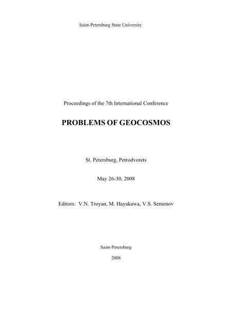
The mean variations in geopotential heights of the isobaric surface 1000 hPa during Forbush decreases<br />
under consideration are presented in Fig.1. The white lines indicate the areas, where the statistical significance of<br />
the deviations is above 0,95 and 0,99 according to the Student t-criterion. As it seen from the figure, a slow<br />
pressure growth takes place near the south-eastern coasts of Greenland on the first days (0/+1 days) after the<br />
Forbush decrease onset. Then, the area of the increasing pressure extends in the north-eastern direction and<br />
reaches its maximum on the +3/+4 days after the Forbush decrease beginning, covering all Scandinavia, the north<br />
of European part of Russia and the Arctic Ocean coasts. The deviations from the undisturbed level in this region<br />
amount to ∼ 60-70 gp.m.<br />
Latitude, deg.<br />
80<br />
60<br />
40<br />
20<br />
80<br />
60<br />
40<br />
20<br />
80<br />
60<br />
40<br />
20<br />
80<br />
60<br />
40<br />
20<br />
-50 0<br />
-1 day<br />
50<br />
0.95<br />
0.99<br />
-50 0<br />
0 day<br />
50<br />
-50 0<br />
1 day<br />
50<br />
-50 0<br />
2 day<br />
50<br />
0.95<br />
0.99<br />
0.99<br />
0.95<br />
0.99<br />
0.95<br />
40<br />
20<br />
0<br />
-20<br />
-40<br />
40<br />
20<br />
0<br />
-20<br />
-40<br />
40<br />
20<br />
0<br />
-20<br />
-40<br />
40<br />
20<br />
0<br />
-20<br />
-40<br />
80<br />
60<br />
40<br />
20<br />
80<br />
60<br />
40<br />
20<br />
80<br />
60<br />
40<br />
20<br />
80<br />
60<br />
40<br />
20<br />
Longitude, deg.<br />
0.95<br />
0.99<br />
0.99<br />
0.95<br />
0.95<br />
0.99<br />
-50 0 50<br />
3 day<br />
0.95<br />
0.95<br />
0.99<br />
0.99<br />
-50 0<br />
4 day<br />
50<br />
0.95<br />
0.99<br />
-50 0<br />
5 day<br />
50<br />
0.99<br />
-50 0<br />
6 day<br />
50<br />
Fig. 1 Mean variations in geopotential heights (in gp.m) of the isobaric level 1000 hPa in the<br />
course of GCR Forbush decreases for 48 events (1980-2006, cold half of year). White lines<br />
show the areas where the effects are significant at 0,95 and 0,99 confidence level. Black and<br />
blue lines show the climatic position of the Arctic and Polar fronts in January, respectively<br />
[Khromov and Petrosyants, 1994].<br />
Variations in geopotential heights of the isobaric levels 1000, 850, 700, 500, 300 and 200 hPa on the +4<br />
day after the Forbush decrease onset, which is the day of the greatest pressure increase, are shown in Fig.2. White<br />
lines show the areas where the effects are significant at 0,95 and 0,99 confidence level according to the Student tcriterion.<br />
We can see a noticeable pressure growth at all the isobaric levels, but the most significant effects take<br />
place near the Earth’s surface. The effect weakens with the increase of the altitude.<br />
The data in Fig. 2 show also the climatic position of the main atmospheric fronts at middle latitudes in<br />
January according to Khromov and Petrociants (1994). Atmospheric fronts are rather narrow transition bands<br />
between air masses with different thermal characteristics which are formed over different kinds of surface. The<br />
8<br />
0.95<br />
0.95<br />
0.99<br />
0.99<br />
40<br />
20<br />
0<br />
-20<br />
-40<br />
40<br />
20<br />
0<br />
-20<br />
-40<br />
40<br />
20<br />
0<br />
-20<br />
-40<br />
40<br />
20<br />
0<br />
-20<br />
-40
Proceedings of the 7th International Conference "Problems of Geocosmos" (St. Petersburg, Russia, 26-30 May 2008)<br />
Arctic front separates in winter the cold Arctic air over Greenland from the warmer air of middle latitudes over<br />
the ocean, whereas the Polar front separates the air mass of middle latitudes from the tropical air mass. The main<br />
atmospheric fronts are of particular interest for the studies, because the cyclonic activity at extratropical latitudes<br />
is closely related to these fronts. Most of extratropical cyclones arise and undergo significant changes in their<br />
evolution namely at the Arctic and Polar fronts. Indeed, the most appreciable pressure deviations are observed in<br />
the regions of the climatic position of these fronts, i.e. in the areas of intensive cyclogenesis. This allows the<br />
suggestion that a possible reason of the observed pressure deviations may be the changes in cyclone and<br />
anticyclone evolution.<br />
Latitude, deg.<br />
80<br />
60<br />
40<br />
20<br />
80<br />
60<br />
40<br />
20<br />
80<br />
60<br />
40<br />
20<br />
Level = 1000 hPa<br />
-50 0 50<br />
Level = 850 hPa<br />
-50 0 50<br />
Level = 700 hPa<br />
0.95<br />
0.95<br />
0.99<br />
0.95<br />
0.99<br />
-50 0 50<br />
0.95 0.99<br />
0.95 0.99<br />
0.99<br />
0.95<br />
0.99<br />
0.95<br />
40<br />
20<br />
0<br />
-20<br />
-40<br />
-60<br />
40<br />
20<br />
0<br />
-20<br />
-40<br />
-60<br />
40<br />
20<br />
0<br />
-20<br />
-40<br />
-60<br />
80<br />
60<br />
40<br />
20<br />
80<br />
60<br />
40<br />
20<br />
80<br />
60<br />
40<br />
20<br />
Longitude, deg.<br />
Level = 500 hPa<br />
-50 0 50<br />
Level = 300 hPa<br />
0.95<br />
0.99<br />
0.95<br />
-50 0 50<br />
Level = 200 hPa<br />
-50 0 50<br />
0.95<br />
0.99<br />
0.95<br />
0.99<br />
Fig. 2 Mean variations in geopotential heights (in gp.m) of the isobaric levels 1000, 850, 700,<br />
500, 300 and 200 hPa on the +4 day after the Forbush-decrease beginning for 48 events (1980-<br />
2006, cold half of year). White lines show the areas where the effects are significant at 0,95<br />
and 0,99 confidence level. Black and blues lines show the climatic position of the Arctic and<br />
Polar fronts in January, respectively [Khromov and Petrociants, 1994].<br />
To check this assumption, the weather chart analysis was carried out. The weather charts provide<br />
comprehensive information about atmospheric conditions at the moment of observation, in particular, about the<br />
spatial distribution of air masses and their characteristics, the atmospheric fronts and the different baric systems<br />
such as cyclones and anticyclones, troughs and crests. An example of the synoptic situation on the +3/+4 days of<br />
the Forbush decrease which started on the 13 January 1988 is presented in Fig.3.<br />
9<br />
40<br />
20<br />
0<br />
-20<br />
-40<br />
-60<br />
40<br />
20<br />
0<br />
-20<br />
-40<br />
-60<br />
40<br />
20<br />
0<br />
-20<br />
-40<br />
-60
Proceedings of the 7th International Conference "Problems of Geocosmos" (St. Petersburg, Russia, 26-30 May 2008)<br />
Fig. 3. Example of synoptic situation on the +3/+4 days of the GCR Forbush decrease starting on<br />
the 13 January 1988.<br />
We can see that on the +3 day (16 January 1988, left panel) the high pressure area (1025 hPa in the<br />
center) is formed over the north of Scandinavia at the cold front of the cyclone with the center over Taimyr<br />
peninsula. The cold front stretches along the Arctic coast of Eurasia. There is also an occluded cyclone over<br />
Greenland, the pressure in its center is 960 hPa. On the next day (right panel) the cold front is displaced to the<br />
south, the pressure in the anticyclone reaches 1030 hPa, its area increases noticeably and covers both Scandinavia<br />
and the north of the European part of Russia. The cyclone near Greenland does not move and rapidly fills up to<br />
980 hPa. Similar processes were found to occur in most cases.<br />
Thus, the results of synoptic analysis showed that, as a rule, after the Forbush decrease onset the<br />
transformation of intensive mobile cold anticyclones into slowly-moving ‘blocking’ anticyclones takes place.<br />
These anticyclones create an obstacle for the transport of air masses from the North Atlantic to the continent. This<br />
process results in the decrease of intensity as well as in the slowing or even in the stop of cyclones, which usually<br />
move to the east (or to the north-east) in the zonal flow. As a result, the pressure over Scandinavia and the north<br />
of the European part of Russia starts to growth.<br />
Latitude, deg.<br />
80<br />
70<br />
60<br />
50<br />
40<br />
30<br />
20<br />
0.3 GV<br />
0.5 GV<br />
0.9 GV<br />
2 GV<br />
3 GV<br />
4 GV<br />
5 GV<br />
0.1 GV<br />
7 GV<br />
9 GV<br />
Polar front<br />
2 GV<br />
11 GV<br />
12 GV<br />
13 GV<br />
14 GV<br />
Arctic front<br />
-80 -60 -40 -20 0 20 40 60 80<br />
Longitude, deg.<br />
gp.m<br />
Fig. 4. Mean variations in geopotential heights (in gp.m) of the isobaric level 1000 hPa on the +4<br />
day after the Forbush-decrease beginning, superposed by the geomagnetic cutoff rigidity (R, GV)<br />
map, and the climatic position of the main atmospheric fronts at middle latitudes in January<br />
[Khromov and Petrociants, 1994].<br />
10<br />
40<br />
20<br />
0<br />
-20<br />
-40<br />
-60
Proceedings of the 7th International Conference "Problems of Geocosmos" (St. Petersburg, Russia, 26-30 May 2008)<br />
According to Shea and Smart (1983), the geomagnetic cutoff rigidities in the areas of most intensive<br />
anticyclone activity vary from ~ 0,2 GV to 0,4 GV (the Arctic front region) and from ~2 GV to 3,5 GV (the Polar<br />
front region), that corresponds to the energies ~ 20−80 MeV and ~ 2−3 GeV, respectively . The geomagnetic<br />
cutoff rigidity map and the climatic position of the main atmospheric fronts at middle latitudes in January<br />
[Khromov and Petrociants, 1994], are shown in Fig. 4. As it seen from the figure, the main atmospheric fronts<br />
under study turn to be in the zones of precipitation of particles with the minimum energy ~20−80 MeV (the<br />
Arctic front) and ~ 2−3 GeV (the Polar front). The intensity of cosmic particles with such energies is strongly<br />
modulated by solar activity that allows considering them as the most probable link between solar activity and the<br />
lower atmosphere. An intensification of anticyclones in the regions of particle precipitations with the indicated<br />
energies seem to provide new evidence that the variations of these particles are involved in the physical<br />
mechanism of solar activity effects on the formation and development of extratropical baric systems.<br />
Conclusions<br />
This investigation showed that Forbush decreases of galactic cosmic rays are accompanied by the<br />
noticeable pressure growth at middle and high latitudes, the most significant effects were found in the regions of<br />
the climatic Arctic front stretching from the Greenland coasts to the Arctic coasts of Eurasia and of the Polar<br />
front in the eastern part of the North Atlantic. The result obtained suggest that the pressure changes associated<br />
with the events under study are due to the changes in the intensity of cyclonic activity (i.e. formation and<br />
development of extratropical cyclones and anticyclones) in these regions.<br />
The synoptic analysis showed that the observed pressure increase in the Arctic front region was really<br />
caused by the changes in the evolution of mobile anticyclones forming in the rear of frontal cyclones. It was<br />
revealed that after the Forbush-decrease onset these anticyclones transformed very often to so called ‘blocking’<br />
anticyclones slowing their movement over Scandinavia and, thus, creating an obstacle for the movement of<br />
North-Atlantic cyclones in the eastern direction. This process contributed to the pressure increase over<br />
Scandinavia. The results obtained are in good agreement with the previous studies by Pudovkin et al. (1997)<br />
who revealed a growth of pressure in all the troposphere at Sodankylä station (Finland) and with the studies by<br />
Tinsley and Deen (1991) who showed a decrease of cyclonic vorticity at middle latitudes associated with<br />
Forbush-decreases of GCR.<br />
We suggest that the cosmic particles having sufficient energies to reach geomagnetic latitudes of the<br />
Arctic front (E ~ 20−80 MeV) and of the Polar front (E ~2−3 GeV) may take part in the processes of cyclone<br />
and anticyclone formation and development in the frontal regions.<br />
References<br />
Kalnay, E., et al. (1996), The NCEP/NCAR 40-Year Reanalysis Project, Bull.of Amer.Met.Soc., 77, 437-472.<br />
Khromov, S.P., and M.A. Petrociants (1994), Meteorology and climatology, Mosk.Gos.Univ., Moscow.<br />
Pudovkin, M.I., and S.V. Babushkina (1992), Influence of solar flares and disturbances of the interplanetary<br />
medium on the atmospheric circulation, J. Atm. Sol.-Ter. Phys, 54 (7/8), 841-846.<br />
Pudovkin, M.I., S.V. Veretenenko, R. Pellinen and E. Kyrö (1997), Meteorological characteristic changes in the<br />
high-latitudinal atmosphere associated with forbush-decreases of galactic cosmic rays, Adv.Sp.Res., 20(6),<br />
1169-1172.<br />
Shea, M.A., and D.F. Smart (1983), A world grid of calculated cosmic ray vertical cutoff rigidities for 1980, in:<br />
18 th International Cosmic Ray Conference Papers, 3, 415-418.<br />
Tinsley, B.A., and G.W. Deen (1991), Apparent tropospheric response to MeV-GeV particle flux variations: a<br />
connection via electrofreezing of supercooled water in high-level clouds?, J.Geophys.Res., 96, 283-296.<br />
Veretenenko, S.V., and I.V. Artamonova (2005), Forbush-decrease of galactic cosmic rays influence on the<br />
cyclone processes intensity at the middle and high latitudes, in: Proc. of IX Int. Solar Physics Conf., (GAO<br />
RAN, Pulkovo, St.Petersburg, 4-9 July 2005), 11-16.<br />
Veretenenko, S.V., and P. Thejll (2004), Effects of energetic solar proton events on the cyclone development in<br />
the Nirth Atlantic, J.Atm.Sol.-Ter.Phys., 66, 393-405.<br />
11
Proceedings of the 7th International Conference "Problems of Geocosmos" (St. Petersburg, Russia, 26-30 May 2008)<br />
INSTABILITY <strong>OF</strong> THIN CURRENT SHEET<br />
A. V. Artemyev 1 , L.M. Zelenyi 1 , H.V. Malova 1,2 , V.Y. Popov 1,3<br />
1 Space Research Institute, RAS, Moscow, e-mail: ante0226@gmail.com<br />
2 Institute of Nuclear Physics, Moscow State University<br />
3 Physics Department, Moscow State University<br />
Abstract. Eigenmodes of thin anisotropic current sheet (TCS) are studied in this work. Growth<br />
rate of kinetic ion-wave resonance instability is found as a function of TCS parameters. It is shown<br />
that there exist two possible polarizations for symmetric and asymmetric modes with positive and<br />
negative values of the growth rate both for sausage-kink and tearing-twisting instabilities.<br />
Introduction. Theory of eigenmodes of current sheet (CS) instability can be used for describing of various<br />
dynamical processes in Earth’s magnetosphere. For example, tearing instability was studied as a reason of<br />
magnetic reconnection of CS (Coppi et al. 1966). Various of drift modes<br />
(Daughton 1999, Artemyev et al. 2008a) can describe oscillation motions of CS (Sergeev et al. 2004,<br />
Petrukovich et al. 2006). But for different models of initial equilibrium one can obtain different values of<br />
frequency and growth rate from linear theory of instability. Therefore it is interesting to study the properties<br />
of CS perturbations that are close to observation data (Runov et al. 2006). In this work we investigate TCS<br />
model (Zelenyi et al. 2004) and we show that the comparison of this model with experimental observation of<br />
CS gives a good result (Artemyev et al. 2008b).<br />
Model of TCS. The model we propose (Zelenyi et.al 2004) contains electron and ion components. In our<br />
approach the parameter is small: bn = Bz B0<br />
< 0.3 ( B0 is the magnitude of the magnetic component Bx ( z ) ),<br />
B 0 ~ 0 ). In this<br />
as a consequence ions can be taken into account as unmagnetised near neutral line of CS ( ( )<br />
case equations of motion might be solved by using quasi-adiabatic integral of motion<br />
(Sonnerup 1971, Buechner and Zelenyi 1989).<br />
I z = ∫ mivz dz<br />
In a case of a constant magnetic field at the edges of the system I z<br />
2<br />
= mi v⊥ ωi<br />
( ωi is gyrofrequency of ions<br />
2 2<br />
in the edges of the system). Therefore, one can use full ion energy 0 i ( ⊥ )<br />
to construct ions velocity distribution in each point of the system (Zelenyi et.al 2004):<br />
2<br />
{ ω ( 0 ω ) }<br />
W = m v� + v 2 + eϕ and invariant z I<br />
f ~ exp − I − W − I − v<br />
(1)<br />
i i z i z D<br />
This velocity distribution corresponds to ion flows moving from the edges of the system toward the center<br />
along magnetic field lines with the velocity v D . Ions turn the direction of motion in neutral plane of CS from<br />
W > ω I ). Ions with such behaviour are called<br />
X to Y direction and then leave the system (it happens if 0 i z<br />
“Speiser” ions. The main parameter characterizing this plasma population is ε = vTi vD<br />
( vTi is thermal ion<br />
velocity). In the case W0 < ωiI<br />
z ions become trapped and their distribution function is taken as thermal<br />
Maxwellian distribution.<br />
Electrons are magnetized everywhere inside CS in the case Bz ≠ 0 . Therefore in our model we use drift<br />
approach for electron component (Zelenyi et.al 2004). In this case electron current density can be written as:<br />
[ E× B]<br />
c c<br />
je⊥ = − enec + 2 2 [ B×∇ ⊥ p⊥e ] + 4 ( p� e − p⊥e<br />
) ⎡ × ( ∇)<br />
⎤<br />
B B B<br />
⎣B B B⎦<br />
(2)<br />
Here e n is the electron density, p⊥e and e p� are perpendicular and parallel pressure components, and<br />
B =<br />
2 2<br />
Bx + Bz<br />
. Last term in (3) corresponds with curvature electron drift and in the central region of CS<br />
2<br />
( B x ( 0 ) ~ 0 ) this term is proportional to Bz − . Because parameter bn = Bz B0<br />
is small the electron current in<br />
the central region of CS is larger than ion. On the other hand ion current density profile is wider than electron.<br />
As a result several different spatial scales are presented in TCS (figure 1).<br />
12<br />
x
Proceedings of the 7th International Conference "Problems of Geocosmos" (St. Petersburg, Russia, 26-30 May 2008)<br />
Tearing instability. Tearing instability is a<br />
symmetrical mode of plasma perturbation (perturbed<br />
component of vector potential A1 ( z) = A1 ( − z)<br />
) which<br />
is periodical along magnetic field direction<br />
~ exp( ikx x − iωt ) . Growing of tearing perturbation is<br />
supported by resonance interaction of unmagnetized<br />
particles with plasma waves in the central region of CS<br />
( B x ~ 0 ). For the first time Harris CS model (Harris<br />
1962) was used for instability investigations where<br />
electrons were considered as resonance particles<br />
(Coppi et al. 1966). But the nonzero normal<br />
component of magnetic field Bz ≠ 0 always is present<br />
in Earth’s magnetosphere. Electrons become<br />
Figure 1. Electron and ion current<br />
magnetised by B z magnetic component and resonance<br />
density and plasma density<br />
interaction is dominated by ions (Schindler 1974,<br />
Galeev and Zelenyi 1976). The stabilization effect of magnetized electrons (Lembége and Pellat 1982)<br />
makes Harris CS stable to tearing perturbation (Pellat et al. 1991).<br />
There exist several models of CS equilibrium which are alternative to Harris CS with Bz ≠ 0 (Sitnov et al.<br />
2006, Birn et al. 2004, Zelenyi et al. 2004). Also one can investigate tearing-like perturbation along<br />
directions which are not coinciding with magnetic field lines and propagate under the angle<br />
θ = arctan ( k y kx<br />
) to it. In our work we study tearing perturbation in model of TCS (Zelenyi et al. 2004) for<br />
which lager store of free energy was found (Zelenyi et al. 2008).<br />
Kink and sausage instability. Symmetric wave perturbation exp{ i − iωt} two values of arctan ( k y kx<br />
)<br />
kr has two well known modes for<br />
θ = . If θ = 0 (direction along magnetic field) perturbation is named tearing and<br />
if θ = π 2 (direction along the current j y ) perturbation is named sausage. Sausage mode was investigated<br />
for Harris CS (Lapenta and Brackbill 1997, Daughton 1999). But several features of structure can be a reason<br />
of the difference in behaviour of this mode in TCS .<br />
Asymmetric mode ( A1 y ( − z) = − A1 y ( z)<br />
) with θ = π 2 is named kink perturbation. This mode is<br />
investigated for Harris CS (Kuznetsova and Zelenyi 1985, Daughton 1999). It was shown that for TCS this<br />
perturbation has larger growth rate than for Harris one and larger period of oscillation (Artemyev et al.<br />
2008a). Because of substantial storage of free energy in TCS model with Bz ≠ 0 the modes with angle not<br />
only θ = π 2 can exist in the neutral plane of this CS. Therefore, it this work we take into account various<br />
modes of instability with different values of angel θ .<br />
Energy principle. Necessary conditions of CS instability. In this section we consider energy function of<br />
( 2)<br />
the second order of perturbation W for TCS and for Harris CS with Bz ≠ 0 . We start from standard<br />
( 2)<br />
equation for W (Schindler 2006):<br />
2<br />
2<br />
( 2) B1 1 f̃ 1 j<br />
W = ∫ dr − ∑ 8π 2 ∫ j ∂f0 j ∂H 0 j<br />
1 ∂j<br />
q<br />
0 2<br />
j res<br />
drdp −∑ 1d d −∑<br />
1 f1 j d d<br />
j 2c<br />
∫ A r p<br />
∂ 0<br />
j c ∫ vA r p<br />
A<br />
(3)<br />
= z i − iωt f̃ = f − ∂f ∂A A<br />
res<br />
− f . The resonance part of perturbed<br />
Here we use ( ) { }<br />
A1 A1 exp kr and 1 j 1 j ( 1 j 0 ) 1 1 j<br />
res<br />
distribution function f 1 j can be obtained for each models of CS independently. In the presence of the<br />
normal component of magnetic field B z electrons are magnetized near the neutral plane and perturbation of<br />
their density corresponds with magnetic field perturbation<br />
Schwartz inequality to rewrite equation (4):<br />
n1 = n0 ( B1z Bz<br />
) . In this case one can use<br />
13
Proceedings of the 7th International Conference "Problems of Geocosmos" (St. Petersburg, Russia, 26-30 May 2008)<br />
2<br />
2<br />
2 1 1 p0 B1z<br />
1 ∂j<br />
q<br />
0 2<br />
j<br />
res<br />
= ∫ + 2<br />
1 1 1 j<br />
8π 2 ∫ −∑ −<br />
Bz j 2c<br />
∫ ∑<br />
∂A0<br />
j c ∫<br />
( ) B<br />
W dr dr A drdp vA f drdp Here we use p n ( z)( T T )<br />
= + . To obtain equation for perturbed vector potential one should take first<br />
0 0 i e<br />
( 2)<br />
variation over W :<br />
2 2<br />
2<br />
d A ⎛ 1 k 1 ∂j<br />
⎞ 0<br />
kx<br />
− 4π 2 ⎜ − ⎟ A1 − 4π<br />
p0 A 2 1ye<br />
y<br />
dz ⎝ 4π<br />
c ∂A0<br />
⎠ Bz 4π<br />
res<br />
= − j<br />
c<br />
2<br />
Here we take into account that B1z = ikx A1<br />
y and ∆ A1 = d A1 2 2<br />
dz − k A 1 , where k = k + k .<br />
2 2 2<br />
x y<br />
2 2<br />
To solve equation (6) for tearing perturbation ( k = k ) one should write the following inequality:<br />
2 2 2 −1<br />
( r) = 4π + − ∂j ∂ A < 0 . In the case U ( ) > 0<br />
U k p k B c<br />
*<br />
1 ~ exp( z k ) −<br />
then ( )<br />
x 0 x z<br />
0 0<br />
x<br />
(4)<br />
(5)<br />
r there exist only trivial solution<br />
2<br />
A and growth rate of instability has negative value. If one use 1 p0 Bz<br />
B B is necessary condition of CS instability. For<br />
f z = . In this case we obtain kL < bn<br />
for tearing instability in Harris CS.<br />
This inequality ( kL < bn<br />
) was before obtained in 1982 (Lembége and Pellat 1982).<br />
In TCS model the shear of bulk velocity vy ( z) is characteristic therefore one can study inequality<br />
2 −2<br />
( ) > ( ) ( ) , which takes the following form ( )<br />
v z u kL b f z<br />
y n<br />
Figure 2. Examination of necessary criteria of CS instability for TCS model.<br />
( ) 1 −<br />
2<br />
Determining the profiles ( ) 0.5ε<br />
( ) ( ) ( )<br />
−1 3 −2<br />
v y T n<br />
−1 3 2 −2<br />
( vy z vT ) 0.5ε<br />
( kL) bn f ( z)<br />
> .<br />
F z = kL f z v z v b as a function of z coordinate one can<br />
find region with Fv ( z ) < 1 in the centre of CS (figure 2). Presence of region with v ( ) 1<br />
exist of possibility of developing of tearing perturbation in TCS.<br />
14<br />
F z < shows that there
Proceedings of the 7th International Conference "Problems of Geocosmos" (St. Petersburg, Russia, 26-30 May 2008)<br />
Sufficient condition of CS instability. To obtain sufficient condition of instability one should find<br />
res res 3<br />
nontrivial solution of equation (5) with resonance term j = e∫ v fi d v . Resonance part of perturbed<br />
res<br />
distribution function f i can be fund by standard way from linearized Vlasov equation (Lapenta et al. 1997,<br />
Daughton 1999, Silin et al. 2002). Also we applies Coulomb calibration for the perturbed vector potential,<br />
div A 1 = 0 . One could consider two different polarizations of perturbations of vector potential A 1 . First<br />
polarization is presented in the form A1 = A1 xe x + A1<br />
ye y (Galeev and Zelenyi 1976, Silin et al. 2002).<br />
Coulomb calibration then imposes the following condition of components of the perturbed vector potential:<br />
A cosθ + A sinθ = 0 . Perturbations with such polarization are suppressed when θ → π 2 . Perturbation<br />
1x y<br />
with another polarization A1 = A1 ye y + A1<br />
ze z (Lapenta and Brackbill 1997) can be developed also for<br />
θ = π 2 . In this paper we will consider below both kinds of polarization.<br />
For the polarization of vector potential 1 A in a form A1 = A1 xe x + A1<br />
ye y , it is more convenient to consider<br />
single equation for its magnitude<br />
A = A + A instead of the system of two equations for each of these<br />
2 2<br />
1 1x 1y<br />
components. It is straight forward, because 1x A and 1y A are linearly coupled (i.e. 1 1 tan<br />
x y<br />
Coulomb calibration:<br />
− −<br />
res<br />
{ ( 1 4π z cos θ ) 0.5 ( y ) cos θ} ( , θ,<br />
, )<br />
2 2 2 2 4 1 2<br />
1 0 0 1 1<br />
A = − A θ ) by<br />
d A dz − k + p B − c ∂j ∂ A A = − j z A t (6)<br />
For another type of polarization A1 = A1 ye y + A1<br />
ze z one could solve the single equation for A 1y like it was<br />
done by Lapenta and Brackbill (1997) for the sausage mode ( θ = π 2 ). Contrary to previous works we<br />
extended our results for perturbations at arbitrary angles (not only θ π 2<br />
= )neutral plane ( , )<br />
− −<br />
res<br />
{ ( 1 0.5 cos θ ) 0.5 ( ) } ( , θ,<br />
, )<br />
2 2 2 2 2 1<br />
1y 0 z y 0 1y 1y<br />
x y propagating:<br />
d A dz − k + p B − c ∂j ∂ A A = − j z A t (7)<br />
Because the resonant current densities,<br />
t<br />
∫<br />
0<br />
( − ) ( )<br />
res<br />
j ~ K t t′ A t′ dt′<br />
1<br />
, depends on<br />
time, equations (6) and (78) could be<br />
considered as evolutionary equations and<br />
could be solved by method of finite<br />
elements (Lapenta and Brackbill 1997,<br />
Daughton 1999). Then one could obtain<br />
corresponding eigenfrequencies and<br />
growth rates as a function of TCS<br />
parameters, wavenumbers k and<br />
propagation angles θ .<br />
The resulting growth rates as a function of<br />
propagation angles θ for both<br />
polarizations are shown in figure 3. As<br />
one can see, both symmetric polarization<br />
modes have equal positive values of Figure 3. Growth rate as a function of angle θ for two<br />
growth rate in the case of tearing polarizations. Parameters have following values:<br />
instability ( θ = 0 ), but asymmetric modes τ = 3 , L = 0.8ρi , kL = 0.3,<br />
b n = 0.1 .<br />
are suppressed when θ → 0 . While the<br />
perturbation angle θ increases perturbation with the polarization A1 = A1 xe x + A1<br />
ye y become suppressed.<br />
But perturbation having another polarization ( A1 = A1 ye y + A1<br />
ze z ) become correspondingly sausage or kink<br />
instabilities ( θ = π 2 ). In the range θ ~ π 2 the perturbation growth rate become larger than the one of<br />
tearing mode ( θ ~ 0 ). Thus the vector potential perturbations in propagating along the direction of the<br />
currents are more probable than perturbation of the tearing mode type (i.e. waves moving along x direction).<br />
Also the asymmetric perturbations at θ = π 2 have larger growth rate than the symmetric one like it was<br />
obtained in Harris CS (Daughton 1999).<br />
15
Proceedings of the 7th International Conference "Problems of Geocosmos" (St. Petersburg, Russia, 26-30 May 2008)<br />
The growth rate of symmetric mode with polarization A1 = A1 ye y + A1<br />
ze z as a function of wavenumber k is<br />
shown in figure 4. As one can see, the range of wavenumbers with positive values of the growth rate is wider<br />
than the one in classical Harris CS (Daughton 1999). Maximum value of the growth rate for different values<br />
kL∈ 0.8,1.8 . Real part of frequency in this region of<br />
of propagation angle belongs to interval [ ]<br />
wavenumbers acquires values ω [ ] ω<br />
∈ 0.01, 0.035 i (this range is the same for both symmetric and asymmetric<br />
modes). These values are much smaller than in the ‘classical’ case of thin Harris CS (Lapenta and Brackbill<br />
1997, Daughton 1999) because real part of frequency corresponds to the diamagnetic drift frequency<br />
ω = k v = kv sinθ<br />
, where v DM is the velocity of diamagnetic drift, and in Harris CS where most of the<br />
*<br />
y DM DM<br />
current is produced by diamagnetic effect vDM ~ dn dz anddensity gradients are much lager than in<br />
anisotropic CS with few embedded layers (Artemyev et al. 2008a).<br />
Discussion and Conclusion. The results of<br />
linear analysis of low frequency wave-like<br />
instabilities in propagating in the vicinity of<br />
neutral plane of TCS are discussed in this<br />
paper. We have shown that unstable modes<br />
could have two different types of<br />
polarization as well as two symmetries. One<br />
of them is suppressed at θ ~ π 2 while the<br />
second has maximum of growth rate at such<br />
direction of propagation (this case<br />
corresponds to the classical sausage mode).<br />
Growth rate as a function of both the<br />
amplitude of wavevector and its direction is<br />
obtained. We have shown that TCS tearing Figure 3. Growth rate as a function of magnitude of<br />
instability might have positive values of wavenumber k for polarizations A = Aye y + Aze<br />
z .<br />
growth rate contrary to the Harris CS with<br />
Bz ≠ 0 (Pellat et al. 1991). Detailed<br />
Parameters have following values: τ = 3 , L = 0.6ρi ,<br />
discussion of this devoted to the investigation of marginally stable TCSs is given in paper by Zelenyi et al.<br />
(2008).<br />
Because the direction of drift velocity for each CS is always predefined (the direction of current) its low<br />
frequency eigenmodes if become unstable should have properties of drifts waves. This characteristic is<br />
similar to the one for Harris CS model (Lapenta and Brackbill 1997, Daughton 1999) but anisotropic TCS<br />
model predicts at least 4-5 smaller characteristic frequency than earlier Harris type models.<br />
Conceptually we would like to stress the point coming from our analysis that perturbations observed within<br />
CS, even if assumed to belong to CS eigenmodes class (non-eigenmode transient events could also exist in<br />
magnetotail), could have complicated structure with mixed polarizations and symmetric/asymmetric<br />
characteristics.<br />
This work was supported in part by the RF Presidential Program for State Support of Leading Scientific<br />
Schools (project no. NIII-472.2008.2), the Russian Foundation for Basic Research (project nos. 08-02-00407,<br />
06-05-90631).<br />
References.<br />
Artemyev, A.V., L.M. Zelenyi, Kh. V. Malova, and V.Yu. Popov (2008a), Effect of the Normal Component<br />
of the Magnetic Field on the Kink Instability of the Earth’s Magnetospheric Current Sheet. Plasma Physics<br />
Report, 34(9), 771-779.<br />
Artemyev, A., Petrukovich A., Zelenyi L., Malova H., Popov V., Nakamura R., Runov A., Apatenkov S.<br />
(2008b), Comparison of multi-point measurements of current sheet structure and modern analytical models.<br />
Annales Geophysicae, 26, 2749–2758.<br />
Birn, Joachim, Schindler, Karl, Hesse, Michael (2004), Thin electron current sheets and their relation to<br />
auroral potentials. J. Geophys. Res., 109(A2), doi: 10.1029/2003JA010303.<br />
Büchner J., and Zelenyi L.M., (1989). Regular and chaotic charged particle motion in magnetotaillike field<br />
reversals: 1. Basic theory of trapped motion. J. Geophys. Res., 94(10), 11821-11842.<br />
16
Proceedings of the 7th International Conference "Problems of Geocosmos" (St. Petersburg, Russia, 26-30 May 2008)<br />
Coppi, B., Laval G., and R. Pellat (1966), Dynamics of the geomagnetic tail. Phys. Rev. Letters., 16(26),<br />
1207-1210.<br />
Daughton, W. (1999), The unstable eigenmodes of a neutral sheet, Phys. Plasmas, 6(4), 1329-1343.<br />
Galeev, A.A., and Zelenyi L.M. (1976), Tearing instability in plasma configurations, Zhurnal<br />
Eksperimental'noi i Teoreticheskoi Fiziki, 70(6), 2133-2151. In Russian.<br />
Harris, E.G. (1962), On a plasma sheet separating regions of oppositely directed magnetic field. Nuovo<br />
Cimento. 23, 115.<br />
Kyznetsova M.M., L.M.Zelenyi, (1985), Stability and structure of perturbations of the magnetic surfaces in<br />
the magnetic transitional layers, Plasma Phys. & Controlled Fusion, 27(4), 363-387.<br />
Lapenta, G., and Brackbill, J.U. (1997), A kinetic theory for the drift-kink instability. J. Geophys. Res.<br />
102(A12), 27,099-27,108.<br />
Lembege B., Pellat R. (1982), Stability of a thick two-dimensional quasineutral sheet. Phys. Fluids., 25(11),<br />
1995-2004.<br />
Pellat, R., Coroniti F. V., and Pritchett, P. L. (1991), Does ion tearing exist? Geophys. Res. Lett. 18, 143–146.<br />
Petrukovich, A. A., Zhang, T. L., Baumjohann, W., Nakamura, R., Runov, A., Balogh, A., Carr, C.(2006),<br />
Oscillatory magnetic flux tube slippage in the plasma sheet. Annales Geophysicae, 24, 1695-1704.<br />
Runov, A., V.A. Sergeev, R. Nakamura, W. Baumjohann, S. Apatekov, Y. Asano, T. Takada, M. Volwerk, Z.<br />
Voros, T.L. Zhang, J.-A. Sauvaud, H. Reme, and A. Balogh (2006), Local structure of the magnetotail<br />
current sheet: 2001 Cluster observations. Annales Geophysicae, 24, 247-262.<br />
Schindler, K. (1974), A Theory of the Substorm Mechanism. J. Geophys. Res., 79(19) , 2803-2810.<br />
Schindler, K. (2006), Physics of Space Plasma Activity. Cambridge University Press, ISBN: 9780521858977.<br />
Sergeev, V., Runov A., Baumjohann W., Nakamura R., Zhang T. L., Balogh A., Louarnd P., Sauvaud J.-A.,<br />
Reme H.(2004), Orientation and propagation of current sheet oscillations. Geophys. Res. Lett., 31(5), doi:<br />
10.1029/2003GL019346.<br />
Silin, I., Büchner J., Zelenyi. L. (2002), Instabilities of collisionless current sheets: theory and simulations.<br />
Physics of Plasmas. 9(4), 1104-1112.<br />
Sitnov, M. I., Swisdak M., Guzdar P. N., Runov A. (2006), Structure and dynamics of a new class of thin<br />
current sheets. J. Geoph. Res. 111(A8), doi: 10.1029/2005JA011517.<br />
Sonnerup, B.U.Ö. (1971). Adiabatic particle orbits in a magnetic null sheet, J. Geophys. Res., 76, 8211-8222.<br />
Zelenyi, L. M., H. V. Malova, V. Yu. Popov, D. Delcourt, and A.S. Sharma (2004), Nonlinear equilibrium<br />
structure of thin currents sheets: influence of electron pressure anisotropy, Nonlinear Processes in<br />
Geophysics, 11, 1-9.<br />
Zelenyi, Lev, Artemyev Anton, Malova Helmi, Popov Victor (2008), Marginal stability of thin current sheets<br />
in the Earth’s magnetotail. Journal of Atmospheric and Solar-Terrestrial Physics. 70, 325-333.<br />
17
Proceedings of the 7th International Conference "Problems of Geocosmos" (St. Petersburg, Russia, 26-30 May 2008)<br />
TRIGGER MECHANISM <strong>OF</strong> SOLAR-ATMOSPHERIC RELATIONSHIP<br />
AND THE CONTRIBUTION <strong>OF</strong> THE ANTHROPOGENIC IMPACT<br />
S.V. Avakyan, N.A. Voronin<br />
All-Russian Scientific Center S.I. Vavilov State Optical Institute<br />
Birgevaja line, 12, St. Petersburg, 199034, Russia, e-mail: avak2@mail.ru, avak@soi.spb.ru<br />
Abstract. A unified approach is suggested to the problem of impact of both space and several<br />
anthropogenic sources on the weather and climate changes. This impact is conducted by<br />
microwave ionospheric radiation with is generated both solar flares and by corpuscular<br />
precipitations from magnetosphere. Precipitations of electrons and proton fluxes from radiation<br />
belts take place during geomagnetic storms and also as result rocket launches, technological<br />
activity and at work of powerful radio transmitters.<br />
We suggest three-stage radio-optical trigger mechanism for the influence of solar flares and geomagnetic<br />
storms on the weather characteristics. The first stage is an increase in generation of the<br />
microwave radiation which penetrates from the ionosphere to the earth surface. The second stage<br />
is a change in the proportion of water vapour to water clusters caused by increased microwave radiation.<br />
The third stage is a change of the atmosphere transparence in the absorption bands of water<br />
vapour and clusters. The atmosphere transparence determines the fluxes of solar irradiance<br />
coming down as well as flux of the thermal radiation coming out from the underlying surface.<br />
These fluxes form the basis of the thermal balance and affect the weather and climate characteristics<br />
of the lower atmosphere.<br />
The maximum of secular cycles solar activity was observed in eighties last century. Since 1985 the<br />
total solar irradiance and ionizing fluxes have been decreasing but geomagnetic activity (aa - index)<br />
has been going up till 2003. Only during the last few years geomagnetic activity also started decreasing.<br />
This means that negative trends have come both for solar and geomagnetic activities. We<br />
suppose that according to our mechanism the natural global warming will go down to lower levels.<br />
Introduction<br />
The physical mechanism for natural global climate changes which happened during the last several 11th<br />
solar cycles is considered. The mechanism explains how agents of solar and geomagnetic activities together<br />
affect low-atmospheric processes: with help the flux of microwaves from ionosphere, which are generated<br />
during solar flares and geomagnetic storms due to the excitation of Rydberg states of atoms and molecules<br />
in upper atmosphere by fast ionospheric electrons. It is here very important for climatic changes, that<br />
the maximum of seculars (near one hundred and near of two hundred years) cycle solar activity was observed<br />
in eighties last century.<br />
In this paper are considered:<br />
1) the novel radiooptical the three-stage trigger mechanism of the solar flare and geomagnetic storms<br />
influence at the weather and climate characteristics. [1].<br />
2) forecasting of future climatic changes – a namely decrease of natural contribution of global warming,<br />
if take into account the sum of solar and geomagnetic activity together.<br />
3) role of the new anthropogenic factor of the weather and climate – the experimentally registered precipitations<br />
of electrons from the radiation belts occurring during the period of work of power transmitters<br />
over the cyclotronic frequencies.<br />
Microwave radiation from ionosphere during solar flares and geomagnetic storms as well as microwave<br />
bursts from the Sun are supposed to control the condensation processes in the low atmosphere and thus<br />
affect the weather. This physical mechanism is based on taking into account the excitation of Rydberg states<br />
of atoms and molecules in generation of the ionospheric microwave radiation and in realization of the<br />
dissociative recombination of cluster ions in troposphere [1].<br />
Recently we can read [2]: “We show that over the past 20 years, all the trends in the Sun that could<br />
have had an influence on the Earth’s climate have been in the opposite direction to that required to explain<br />
the observed rise in global mean temperatures... Our results show that the observed rapid rise in global mean<br />
temperatures seen after 1985 cannot be ascribed to solar variability, whichever of the mechanisms is invoked<br />
and no matter how much the solar variation is amplified”. Indeed, since 1985 the total solar irradiance (this<br />
irradiance is the total solar energy flux received at the top of the Earth’s atmosphere) and EUV/X-ray ionizing<br />
fluxes have been decreasing. But geomagnetic activity (aa - index) has been going up till 2003 (+ 0.3 % /<br />
year), Fig. 1. Only during the last few years (on October 2007) geomagnetic activity also started decreasing<br />
(- 5.7 % / year). This means that negative trends after 2003 have come both for solar and geomagnetic activi-<br />
18
Proceedings of the 7th International Conference "Problems of Geocosmos" (St. Petersburg, Russia, 26-30 May 2008)<br />
aa-index<br />
40<br />
35<br />
30<br />
25<br />
20<br />
15<br />
1980 1985 1990 1995 2000 2005<br />
Years<br />
Fig. 1. Trends of the monthly аа-index of geomagnetic activity<br />
before and after 2003.<br />
ties. We suppose that according to our<br />
mechanism the natural global climate<br />
changes will go down to lower levels.<br />
There are also the change of sign for<br />
next trends of atmospheric parameters before<br />
and after 2000-2001:<br />
- the Earth’s albedo decreased during the<br />
period 1984 – 2000/1 and increase after the<br />
year 2000/1 [3],<br />
- the content of water vapour increased in<br />
the atmospheric depth during the period<br />
1980 – 2000 and decrease after the year<br />
2001 (Kyrghyzstan, lake Issyk-kul station<br />
[4]),<br />
- the total contents of ozone these decades,<br />
on the contrary, decreased, that has led to<br />
growth of a erythemal radiation in day time<br />
which also has started to decrease only with<br />
year 2000, then the content of ozone is increase<br />
[5].<br />
Change of a sign on trend of total influence<br />
of solar and geomagnetic activity in<br />
generation of microwave radiation has actually occurred on 1-3 years earlier 2003, as was reflected in terms<br />
of change of signs in trends of the contents vapour of water, methane and ozone.<br />
About the novel radiooptical trigger mechanism of solar-weather and climate links<br />
In according to [6] it is necessary to propose the unknown trigger mechanism of ionospheric disturbance<br />
downward transfer into the troposphere under the action of the solar and geomagnetic activity factors<br />
(solar ionizing radiation and corpuscular fluxes from radiation belts) because the natural energy of weather–<br />
climate phenomena is very high. Avdyushin and Danilov [6] justified than such a necessity is related to the<br />
fact that the energy of the short waves (including the ionizing range) solar radiation, as well as that of corpuscles<br />
(electrons) from radiation belts and solar protons, cannot directly affect the troposphere because<br />
these fluxes do not reach the troposphere, being usually absorbed at much higher altitudes. Therefore, the effect<br />
of the solar ionizing radiation and corpuscular fluxes on the mesosphere and thermosphere should be<br />
somehow transferred downward, to the troposphere. Indeed, the mechanism of the effect of increasing solar<br />
activity on weather characteristics during geomagnetic disturbances due to the known Forbush decrease in<br />
the intensity of galactic cosmic rays was discovered (see [7] and references therein). However, these researchers<br />
repeatedly noted that solar flares, which lead a geomagnetic disturbance - magnetic storm - by approximately<br />
two days, also affect the weather characteristics, first of all, cloudiness. The effect of an increase<br />
in the UV (and X-ray) flux is registered several hours after a solar flare. This is directly related to the response<br />
of the degree of atmosphere transparency to the appearance of an enhanced flux of electromagnetic<br />
(UV) flare emission, when accompanying fluxes of the disturbed solar wind and SCRs have not yet reached<br />
the Earth’s orbit [7].<br />
During the last decades the influence of galactic cosmic rays (GCR) and solar cosmic rays (SCR) on<br />
the cloudness has been studies in detail. The factors of influence are Forbush decrease of GCR and sporadic<br />
increase of SCR. However these events are rare. For instance, geomagnetic storms (with Kp more than 5)<br />
occur 20-80 times per year and solar flares (class greater than M5) take place 50 times per year [8] whereas<br />
Forbush decrease of 3 % and more occurs only 2-4 times per year and solar proton events at energy than 100<br />
MeV take place 5 times per year that is approximately ten times lesser.<br />
We propose to solve this problem in a new way by introducing a “three-stage trigger.” The first stage<br />
is transformation of the energy factors of solar (increased flux of ionizing radiation) and geomagnetic (precipitating<br />
corpuscles from radiation belts) activities in the ionosphere into the flux of microwaves, penetrating<br />
to the Earth’s surface within the troposphere. This is a direct trigger (initiating triggering mechanism)<br />
since direct information relation between the upper atmosphere and the entire troposphere originates precisely<br />
during this stage, which was previously ignored in the solar–terrestrial coupling [9]. The second stage<br />
is regulation of the production and destruction rates of water cluster ions at altitudes where the condensation<br />
19
Proceedings of the 7th International Conference "Problems of Geocosmos" (St. Petersburg, Russia, 26-30 May 2008)<br />
mechanism operates and initiates the generation of cloud and aerosol layers in the lower atmosphere (at altitudes<br />
higher than 3–4 km; i.e., in the zone of influence of galactic cosmic rays) and stratosphere (in the zone<br />
of SCR absorption) [10]. In this stage taking into account Rydberg states excitation at the preliminary stages<br />
of association and dissociation of clusters (as well as ionized clusters) of water vapour and carbon dioxide.<br />
The rates of association and dissociation processes depend strongly on the magnitude of the Rydberg state<br />
orbital quantum number. An increase in the orbital quantum number by one results in a decrease of crosssections<br />
of the dissociation processes by an order of magnitude. According to the developed theory [9]. this<br />
increase in the quantum number is caused by stimulated absorption of the ionospheric microwave radiation<br />
quanta as well as solar radiobursts radiation quanta during the periods of increased solar and geomagnetic activity<br />
(or anthropogenic precipitation impact).<br />
The third stage consists in the evident role of formed clouds and aerosol layers in weather–climate<br />
phenomena via absorption and reflection of certain part of the solar radiant energy and thermal flux from the<br />
underlying surface by these formations [10]. There is various role cloudiness in global warming. According<br />
to [11], the net radiative properties of a cloud are mainly depend on its altitude and optical thickness. Optically-thin<br />
clouds at high and middle altitudes cause a net warming due to their relative transparency at short<br />
wavelengths but opacity in the IR region, whereas thick clouds produce a net cooling due to the dominance<br />
of the increased albedo of short-wave solar radiation, and according to [12], the role of high clouds in the radiation<br />
budget of the earth-atmosphere system depends on optical depths; high thin cloud acts to warm the<br />
atmosphere, while high thick cloud cools. Thus, the decrease in high clouds can reduce both the warming<br />
and cooling effect to the system. But it is clear that because of relatively low power of the ionospheric microwave<br />
radiation (in comparison with atmospheric energy) its influence on the clusterization leads to formation<br />
of optically-thin clouds at the high altitudes.<br />
On the whole, the proposed three stage physical mechanism is an intensifying process since a low energy<br />
of cosmic factors regulates fluxes of incoming and outgoing radiation in the lower atmosphere owing to<br />
strong energy variability. According to numerous calculations [7, 10], even 6% weakening of the solar radiant<br />
energy flux due to reflection and absorption at altitudes of several kilometers can explain the observed<br />
contribution of solar and geomagnetic activities to weather phenomena. In addition, resonance absorption<br />
can participate in this process because the characteristic microwave emission of ionospheric nitrogen and<br />
oxygen molecules in Rydberg transitions in the lower atmosphere by Rydberg excited nitrogen and oxygen<br />
molecules participating (as an ambient gas) in collisional dissociative recombination of cluster ions from water<br />
vapor and carbonic acid molecules [13].<br />
We emphasize that all stages of the proposed novel radiooptical mechanism are experimentally confirmed:<br />
(i) the microwave ionospheric emission, which intensifies during solar and magnetic storms, was detected<br />
in [14, 15];<br />
(ii) the regulation of humidity at altitude higher than 3 km by the solar microwave emission and flares<br />
was registered in [16, 17];<br />
(iii) a direct influence of solar flares and magnetic storms on the total cloudiness is distinctly registered<br />
[18, 19, 20].<br />
Our contribution consists in that we determined the mechanism of generation of the ionospheric microwave<br />
emission in transitions between highly excited (Rydberg) states and used the processes of dissociation<br />
and association of complex ions well known in physics of atomic collisions [13, 21, 22, 23] via intermediate<br />
Rydberg levels. In the case of association (i.e., formation of clusters), the process proceeds through the<br />
addition of proton to parent molecules owing to their high affinity to proton. Produced ions are neutralized<br />
when electron is trapped at a Rydberg orbital. The orbital moment, the value of which can change during absorption<br />
of quanta of the microwave emission from the ionosphere, is the main characteristic of Rydberg levels<br />
affecting the rate of the considered elementary processes.<br />
Rydberg microwave emission of ionosphere during precipitation of electrons from the radiation<br />
belts caused by radio transmitters<br />
Industrial greenhouse effect is usually suggested as a cause of global rise of the surface temperature<br />
over the last few decades. In this paper we propose to draw attention the new anthropogenic component – influence<br />
of powerful radio transmitters (navigation and communication) on the particles in radiation belts of<br />
the Earth. This anthropogenic factor affects mainly the electrons from inner and outer belts over the cyclotronic<br />
frequencies i.e. frequencies of the Larmor precession. These frequencies belong to very low frequency<br />
(VLF) range: from few to few tens kilo Hertz.<br />
20
Proceedings of the 7th International Conference "Problems of Geocosmos" (St. Petersburg, Russia, 26-30 May 2008)<br />
Surface transmitters with such frequency have power up to 1 Mw that cause precipitations and result<br />
in optical emission above the transmitter. Intensity of these emissions is of the same scale with the aurora of<br />
the class two or more in the international IBC II system. Thus, precipitations simulated by VLF transmitters<br />
we suggest to consider as anthropogenic analogue of the aurora caused by magnetic storm.<br />
Let us estimate contribution of this phenomenon into microwave radiation of ionosphere, which according<br />
to experiment [1 16, 17] and its interpretation suggested in [1, 24] could control processes of condensation<br />
and cloud generation in the lower atmosphere. Previously, we considered global geomagnetic<br />
storms in the problem “Sun-weather” [24] and showed that during geomagnetic storms microwave radiation<br />
from Rydberg states, caused by ionospheric fast electrons (secondary electrons and Auger electrons), controls<br />
rate of cluster generation as well as during solar flares.<br />
We take into account results [13] connected with influence of the orbital quantum number (l) of the<br />
Rydberg state on the rate of dissociative recombination of cluster ions. These results show that this rate decrease<br />
when high l levels are filled when strong fluxes of the microwave radiation appear [1, 24]. This could<br />
activate cyclonic activity [25]. Moreover generation of optically thin clouds of the upper layer might cause<br />
warming of the near surface air [11].<br />
Thus we can make very important for the modern climatology conclusion that two important features<br />
of the modern climatic change: (a) global warming and (b) permanent increase in cyclone number (192 cyclones<br />
from 1970 to 1992 and 162 over the next 10 years [25, 26]) have the same nature – global increase of<br />
the number and power of VLF transmitters particularly near maritime coast regions where the cyclogenesis<br />
takes place. This conclusion is based on analysis on intensity of the stimulated electronic precipitations<br />
which are comparable with the precipitations during the global geomagnetic storms. Results of measurements<br />
performed by the satellite DEMETER [27, 28] confirm very high extent of disturbance of radiation<br />
belts and ionosphere during night above the zone of work of VLF transmitters both in Northern Hemisphere<br />
(transmitter NAA in USA with coordinates 44°39 N, 67°17 W), and in Southern Hemisphere (transmitter<br />
NWC in Australia with coordinates 21°47 S, 114°09 E). Areas of the stimulated electronic precipitations and<br />
areas of perturbed ionosphere are linked either with the magnetic force line at which the surface VHL transmitter<br />
is situated or with the magnetic line at which effect of radio wave on the pitch angle of electron, captured<br />
in radiation belt, takes place. In full agreement with the law of latitudinal drift in dipole magnetic field<br />
there is some expanding of the perturbed region eastward thus area of the stimulated perturbations reach a<br />
half of million of square kilometers [28]. Every time perturbation of less scale are observed in magnetic conjugate<br />
area. In accordance with our calculations [29] rate of the optical excitation of ionosphere in the conjugate<br />
point and hence, generation of microwave radiation from Rydberg states reaches 10 % of the effect in<br />
the point of the transmitter work. Intensity of precipitations corresponds to the main phase of geomagnetic<br />
storm. This conclusion is made by us after comparison of the data [27, 28] considering the scale [8], with the<br />
results of measurements of fluxes of electrons precipitating from radiation belts during global geomagnetic<br />
storms performed by satellites “Kosmos-348” [ 30] and “Kosmos-381” which had radiometric equipment<br />
made in State Optical Institute [31]. Actually, according to [31, 32] increases in electronic fluxes, precipitating<br />
to middle latitudes from radiation belts, occur during periods on 2-3 hours over the main and recovery<br />
phase with energies at least 300 times larger than 2.5 and 25 KeV. This regards also to latitudes more than<br />
45° for both day and night conditions in both hemispheres. But just these increases of electron precipitation,<br />
stimulated by work of VFL transmitter are registered by DEMETER satellite [27] even over the lower latitudes.<br />
Experiment [27] showed also that stimulated precipitations correlate well with the level of geomagnetic<br />
perturbation. Fluxes, registered by DEMETER are few order of magnitude higher than levels measured<br />
by the satellite “Oreol-2” for the same energy of electrons in the work [33] for discrete forms of aurora.<br />
Thus precipitation of electrons from radiation belts, registered over periods of VFL transmitters have<br />
fluxes close to that from the global magnetic storm. Such storm is accompanied by intensive emission of all<br />
the upper atmosphere [29] which is aurora. Hence, according to results of our investigation [1, 24, 9, 34]<br />
these simulated precipitations of electrons to ionosphere should cause excitation of Rydberg states with the<br />
corresponding emission of microwave radiation with intensity up to 10 –12 – 10 –11 W сm –2 [24]. It should be<br />
noted, however, that we have not enough information on the spectra of electrons precipitating due to influence<br />
of VLF transmitters [27, 28, 35, 36] that brings some limitations in energy estimations. High altitude<br />
experiments [1, 24] showed that microwave emission in 2-10 cm range might influence process of cluster<br />
generation in the lower atmosphere. According to our hypothesis [1, 24] that should reflect in changes of the<br />
weather and climate parameters. Since radio and VLF transmitters are both products of the industrial activity<br />
of 20 th century probably it is necessary to take into account its geography and working regime when research<br />
solar-weather and solar-climate phenomena.<br />
21
Proceedings of the 7th International Conference "Problems of Geocosmos" (St. Petersburg, Russia, 26-30 May 2008)<br />
Conclusion<br />
The new radiooptical mechanism of the action of solar and geomagnetic activity on the weather and<br />
the climate is substantiated. Suggest integral approach to the problem of the control of weather and climatic<br />
changes by both the natural - space sources and by some anthropogenic (technogenic) actions. In this case is<br />
examined the united agent of this control - microwave emission of the terrestrial ionosphere, which appears<br />
with atoms and molecules excitation of gases of the upper atmosphere by fast ionospheric electrons into the<br />
highly excited (Rydberg) states. Fast ionospheric electrons with the energies more than 10 - 15 eV are<br />
formed with the photoionization of the upper atmosphere under the effect of X-ray and extreme UV solar radiation,<br />
with the corpuscular precipitations both in the period of geomagnetic storms and under the anthropogenic<br />
influences. The latter (emission of powerful radio stations, electric power lines, starting space rockets,<br />
industrial activity) ensure the locality of precipitations (because the most of them induce VLF emissions)<br />
and, correspondingly, the local action of the microwave radiation of the ionosphere on the weather characteristics.<br />
Additionally locality they ensure coastal effect, and thunderstorms, is possible also connection with<br />
breakings of the earth's crusts, the centers of the preparation of earthquakes.<br />
The negative trends after 2003 have come both for solar and geomagnetic activities. We suppose that<br />
according to our mechanism the natural global climate changes will go down to lower levels. Role of the new<br />
anthropogenic factor of weather and climate changes – the experimentally registered precipitations of electrons<br />
from the radiation belts occurring during periods of work of powerful transmitters over the cyclotronic<br />
frequencies – also is discussed.<br />
Acknowledgements<br />
The authors would like to thank for the moral support the foreign collaborators of the International<br />
Science and Technology Center project #3878: A.D. Aylward, APL/UCL. UK; A. Belehaki, NOA, Greece; A.<br />
Hilgers, ESA/ESTEC, Netherlands; J. Lilensten, LPG, France.<br />
References<br />
1. Avakyan, S.V., N.A. Voronin (2006), Condensation Process in the Low Atmosphere and Microwave Radiation<br />
of the Sun and Ionosphere, in: Proceeding of the VI International Conference “Problem of Geocosmos”.<br />
2006. SPbSU. 24-28.<br />
2. Lockwood, M. and C. Frohlich (2007), Recent opposite directed trends in solar climate forcing and the<br />
global mean surface air temperature, Proc. Royal Soc. A., doi: 10.1098/rspa.2007.1880.<br />
3. Climate change. Scientific assessment and policy analysis. Ed. R van Dorland, 2006, 154 pp.<br />
4. Arefiev, N.N. et al. (2006), Water vapour in atmospheric dept of North Tien Shan, Physics of Atmosphere<br />
and Ocean (in Russian), 48, 5, 803-815.<br />
5. Feister, U., J. Junk, and M. Woldt (2008), Long-term solar UV radiation reconstructed by Artificial Neural<br />
Networks (ANN), Atmos. Chem. Phys. Discuss., 8, 453–488.<br />
6. Avdyushin, S.I. and A.D. Danilov (2000), The Sun, Weather, and Climate: A Present Day View of the<br />
Problem (Review), Geomagn. Aeron. 40 (5), 3–14 [Geomagn. Aeron. 40, 545–555].<br />
7. Pudovkin, M.I. and O.M. Raspopov (1992), Mechanism of the Effect of Solar Activity on the State of the<br />
Lower Atmosphere and Meteorological Parameters: A Review, Geomagn. Aeron. 32 (3), 1–22.<br />
8. S.E.C. User Notes. Issue 28. January. 2000. 7 pp.<br />
9. Avakyan, S.V. and N.A. Voronin (2007), On the Possible Physical Mechanism of the Effect of Solar and<br />
Geomagnetic Activity on Phenomena in the Lower Atmosphere, Issled. Zemli Kosm., 2, 23–30.<br />
10. Kondrat’ev, K.Ya. and G.A. Nikol’skii (1995), Solar Activity and Climate. 1. Observational Data. Condensation<br />
and Ozone Hypotheses, Issled. Zemli Kosm., 5, 3–17.<br />
11. Kirkby, J., and A. Laaksonen (2000), Solar variability and clouds, Space Sci. Rev., 94, 1/2, 397-403.<br />
12. Tsushima, Y. (2005), Report of the 2nd International SOWER Meeting, SPARC Newsletter, 24, 24.<br />
13. Bates, D.R. (1981), Electron-ion recombination in an ambient molecular gas, J. Phys. B., 14, 18, 3525-<br />
3534.<br />
14. Forsyth, P.A., W. Petrie, and B.W. Currie (1950), On the Origin of Ten Centimeter Radiation from the<br />
Polar Aurora, Canad. J. Res., Ser. A, 28 (3), 324–335.<br />
15. Bondar’, L.N., K.M. Strezhneva, and V. S. Troitsky (1975), Sporadic Background Radioemission, Solar<br />
Activity, and Auroras, Astron. Vestn., 9 (4), 210–217.<br />
22
Proceedings of the 7th International Conference "Problems of Geocosmos" (St. Petersburg, Russia, 26-30 May 2008)<br />
16. Krauklis, V.L., G.A. Nikol’skii, M.M. Safronova, E.O. Shults (1990), On the conditions of appearance of<br />
abnormal peculiarities of aerosol attenuation of ultra-violet radiation under high transparency of the atmosphere,<br />
Optics of Atmosphere (in Russian), 3, 3, 227-241.<br />
17. Nikol’skii, G.A., E.O. Shults (1991), Time-spectral variations of the residual attenuation in the ultra-violet<br />
range of spectrum, Optics of Atmosphere (in Russian), 4, 9, 961-966.<br />
18. Dmitriev, A.A. and T.Yu. Lomakina (1977), Cloudiness and Space X Rays,” in Solar Activity Effects in<br />
the Lower Atmosphere, Ed. by L.R. Rakipova (Gidrometeoizdat, Leningrad, ), 70–77 [in Russian].<br />
19. Veretenenko, S.V. and M.I. Pudovkin (1994), Effects of GCR Forbush Decreases in Total Cloudiness<br />
Variations, Geomagn. Aeron. 34 (4), 38–44.<br />
20. Veretenenko, S.V. and M.I. Pudovkin (1996), Variations of Total Cloudiness during Solar Cosmic Ray<br />
Events, Geomagn. Aeron. 36 (1), 153–156 [Geomagn. Aeron. 36, 108–111].<br />
21. Mark, T.D. and A.W. Castleman, Jr. (1985), Experimental Studies on Cluster Ions, Adv. At. Mol. Phys.<br />
20, 65–172.<br />
22. Biondi, M.A. (1982), Electron–Ion Recombination in Gas Phase, Appl. At. Coll. Phys., Ed. by E.W.<br />
McDaniel and W. L. Nighan, Vol. 3, pp. 173–189.<br />
23. Gallas, J.A.C., G. Leuch, H. Wallher, and H. Figger (1985), Rydberg Atom: High Resolution Spectroscopy<br />
and Radiation Interaction Rydberg Molecules, Adv. At. Mol. Phys., 20, 413–466.<br />
24. Avakyan, S.V., N.A. Voronin (2006), Possible mechanisms for the influence of heliogeophysical activity<br />
on the biosphere and the weather, Opticheski Zhurnal, (J. Opt. Technol. – in Englich, 73, 4, 281-285), 2006, 73,<br />
4, 78-83.<br />
25. Ivanov, K.G. (2007), Correlation between tropical cyclones and magnetic storms over the 23 th cycle of solar<br />
activity, Geomagn. and aeronomy., 47, 3, 394-398.<br />
26. Golitsyn, G.S. (1997), Statistics and energy of tropical cyclones, Dokl. RAS, 354, 4, 535–538.<br />
27. Sauvaud, J.A., A.R. Maggiolo, C. Jacquey, M. Parrot, J.-J. Berthelier, R.J. Gamble, and C.J. Rodger (2008),<br />
Radiation belt electron precipitation due to VLF transmitters: Satellite observations, Geophys. Res. Lett., 35,<br />
L09101. doi:10.1029/2008GL033194.<br />
28. Parrot, M., J.A. Sauvaud, J.J. Berthelier, and J.P. Lebreton (2007), First in-situ observations of strong ionospheric<br />
perturbations generated by a powerful VLF ground-based transmitter, Geophys. Res. Lett., 34, L11111.<br />
doi:10.1029/2007GL029368.<br />
29. Avakyan, S.V. (2001), Impact of the impulse X-ray source on the optics of upper atmosphere considering<br />
the Auger effect, Opticheski Zhurnal, (J. Opt. Technol. – in Englich), 68, 4, 5-11.<br />
30. Lashtovichka, J. (1980), Precipitation of energetic (E=20-150 KeV) electrons over the middle latitudes,<br />
Geomagn. and Aeronomy, 20, 5, 800-883.<br />
31. Avakyan, S.V., M.P. Bolgartseva, A.I. Efremov, I.A. Krinberg, A.P. Kulakov, V.S. Petrov, A.L. Podmochensky,<br />
I.M. Pribylovsky, G.V. Sazonov, Yu.N. Shaulin (1974), The fluxes of electrons during the magnetic<br />
storm 14-15 December 1970 according to data of the satellite “Kosmos-381”, Issledovania Geomagn. and aeronomy.,<br />
32, 158-161.<br />
32. Avakyan, S.V., A.I. Vdovin, V.F. Pustarnakov (1994), Near-Earth space ionization and penetration radiations,<br />
Handbook, St. Petersburg, Gidrometeoizdat, 501 p.<br />
33. Val'chuk, T.E., Yu.I. Gal'perin, Zh. Kran'e, L.M. Nikolaenko, Zh.-A. Sovo, Ya.I. Fel'dshtein (1979), Diffusion<br />
auroral zone. IV. Latitudinal pattern of precipitation of the auroral particles into ionosphere and structure<br />
of the plasma sheath in the magnetospheric tale, Kosmicheskie Issledovanya, 17, 4, 559-579.<br />
34. Avakyan, S.V (2008), Physics of the solar-terrestrial connections: results, problems and new approaches,<br />
Geomagn. and Aeronomy, 48, 4, 1-8.<br />
35. Inan, U.S., T.F. Bell, J. Bortnik, J.M. Altbert (2003), Controlled precipitation of radiation belt electron, J.<br />
Geoph. Res., 108. A5, 1186.<br />
36. Datlowe, D. (2006), Differences between transmitter precipitation peaks and storm injection peaks in lowaltitude<br />
energetic electron spectra, J. Geoph. Res., 111, A12, 202.<br />
23
Proceedings of the 7th International Conference "Problems of Geocosmos" (St. Petersburg, Russia, 26-30 May 2008)<br />
MAGNETOMETRIC SPECTRA <strong>OF</strong> AURORAL CURRENTS COMPARED<br />
WITH THE DOPPLER RADAR MEASUREMENTS<br />
V.I. Badin<br />
Pushkov Institute of Terrestrial Magnetism, Ionosphere, and Radio Wave Propagation,<br />
IZMIRAN, Troitsk, Moscow Region, 142190, Russia<br />
Abstract. Doppler radar measurements have revealed the enigmatic frequencies of 1.3, 1.9, 2.6,<br />
3.2–3.4 and probably 0.6–0.8 mHz associated with the auroral activity. The frequencies are nearly<br />
invariant, i.e. repetitively observed at independent activity events. This study applies the spectral<br />
analysis to the 10-second magneto-difference data obtained by the IMAGE magnetometer<br />
network. The proposed technique analyzes events of moderate to very low activity of the auroral<br />
electrojet observed at the southward and northward IMF. Each selected event, except that of the<br />
lowest activity, displayed a quasi-stationary auroral arc, with its position being retained within a<br />
narrow interval of latitudes. The magneto-difference data used consist of the differences between<br />
the meridional components of the magnetic fields detected by neighboring magnetometers of the<br />
meridional array of instruments. Distinct equidistant harmonics can be revealed by the<br />
spectrograms. Their spectral peaks indicate different frequencies varying from case to case, but the<br />
frequency distances between adjacent peaks tend to coincide with or closely approach the invariant<br />
Dopplerometric frequencies. An important new feature is that the lower frequencies dominate at<br />
southward IMF while higher at northward. This fact indicates that the ULF signals observed at the<br />
auroral activity cannot be explained by the MHD modes solely. The proposed explanation<br />
interprets the low-frequency harmonics as the spectra of the auroral currents generated by some<br />
rotating sources associated with the magnetospheric convection. The spectrograms obtained for the<br />
very low activity demonstrate a pattern that can be attributed to the MHD spectrum alone. In<br />
general, the ULF spectra observed apparently contain the low-frequency harmonics of some<br />
intramagnetospheric sources and the MHD response to both internal and external sources.<br />
Introduction<br />
The Doppler radar and magnetometric measurements, carried out at high latitudes during periods of<br />
the considerable auroral activity, have revealed some discrete frequencies, namely those of 1.3, 1.9, 2.6, 3.2–<br />
3.4 and probably 06–0.8 mHz [1, 2]. These frequencies demonstrate significant stability or invariance; i.e.<br />
nearly identical frequencies are repetitively observed at independent activity events. To reveal these<br />
frequencies statistically in the magnetometric data, an additional filtering, which extracts highly polarized<br />
signals typical for the magnetic field line resonance, is usually used [1-3]. A critical analysis of the highlatitude<br />
magnetometric data undertaken in [3] questioned the stability of the discrete frequencies revealed. At<br />
the same time, the stability of these frequencies was surprisingly supported by the low-latitude (L=1.6)<br />
observations [4].<br />
The magnetohydrodynamic (MHD) modes of the magnetospheric cavity located between the<br />
magnetopause and the plasmapause were proposed for an explanation of the physical origin of these<br />
signals [2]. However, the well-known theory of such MHD modes treated as coupled compressionaltransverse<br />
oscillations [5] and the numerical computations of magnetospheric dipole MHD spectra [6]<br />
indicate significantly higher frequencies for these modes. Namely, the frequencies of all modes in these<br />
spectra must exceed 5 mHz, since the compressional waves propagating along the shorter transverse size of<br />
the magnetospheric cavity add to the spectrum the frequencies which are higher than those of the transverse<br />
waves propagating along the magnetic field lines. Thus, the MHD spectra of these modes must be shifted<br />
into higher frequencies, and the shift must exceed the frequency distance between successive spectral<br />
components determined by the quantization step of transverse waves.<br />
The contradiction with the theory, in fact, leaves the origin of the discrete auroral frequencies<br />
unknown. On the other hand, the frequencies of the range can be associated with a direct influence of the<br />
solar wind and explained by small changes in the Chapman-Ferraro current induced by variations in the<br />
dynamic pressure of the solar wind [7, 8], although such explanations require some additional reasons for the<br />
invariance or stability of the discrete auroral frequencies. The goal of the present work is to apply a special<br />
spectral analysis to the magnetometric data, in order to examine the origin and stability of the discrete<br />
frequencies revealed.<br />
24
Proceedings of the 7th International Conference "Problems of Geocosmos" (St. Petersburg, Russia, 26-30 May 2008)<br />
Data selection and processing<br />
To apply spectral analysis, the time series studied must approach stationary as closely as possible.<br />
Trying to satisfy this requirement, we can select the auroral events in which the auroral arcs remain quasistationary,<br />
being retained within narrow intervals of latitudes. The all-sky-camera (ASC) keograms recorded<br />
over long activity periods can be very helpful for this purpose. Figure 1 showing the Longyearbyen keogram<br />
(negative) for 17.01.2000 presents a pertinent example. We can see that the auroral arc continually moves<br />
Fig. 1. Keogram shows the aurora retained in a narrow latitudinal interval during 20:00-00:00 UT<br />
along the meridian, being nevertheless retained within a comparatively narrow interval of latitudes. The<br />
meridional motion of the arc introduces the low-frequency noise into the magnetometric data, and this noise<br />
severely impedes the analysis.<br />
The subsequent spectral analysis is executed as follows. For the every pair of neighboring<br />
magnetometers in the meridional array of instruments, the detected meridional magnetic fields are subtracted<br />
from each other forming the magneto-difference signals. These magneto-difference signals eliminate<br />
contributions of distant sources of magnetic fields thus extracting the fields of the nearest sources, which<br />
predominantly are the Hall currents flowing in the ionosphere at the given latitudes. Further, the periodogram<br />
analysis using the Tukey-Hanning spectral window is applied, with the width (resolution) of the window<br />
being individually adjusted for each pair of magnetometers that is for each latitudinal interval. For this<br />
purpose, the analysis is formulated as solving an inverse problem of searching for the spectral window<br />
resolution that gives us the most probable equidistant spectral peaks fitted to the data.<br />
The proposed technique can be risky, of course, when the equidistant spectral model becomes<br />
inconsistent with the physics of the phenomena in study. On the other hand, the equidistant or nearly<br />
equidistant spectra are very typical for numerous physical generators and resonators which can be probable<br />
sources of discrete spectra. There is a little probability that the equidistant spectrum turns out to be<br />
completely inconsistent with the physics. Nevertheless, to take account of opposite situations, an alternative<br />
formulation of the inverse problem is in searching for the most prominent spectral peaks resembling the<br />
Fejer kernel, since we seek for discrete frequencies. In either case, the proposed technique can be quite<br />
appropriate when we have convincing physical reasons to expect some discrete equidistant spectra in the<br />
signals detected. Approximate solutions of the inverse problem can be found by the trial and error method.<br />
We can accelerate the trial and error procedure reducing the spectral resolution successively, until we find<br />
the lowest applicable resolution, below which the spectrum starts to disappear. Some additional reasons for<br />
this technique can be found in [9].<br />
Results and discussion<br />
The first event subjected to the examination is a period of a rather low activity of the auroral<br />
electrojet indicated by the IMAGE activity index IE0 and Kp=0+, while the solar wind<br />
parameters by the density N=3cm -3 and velocity V=700km/s. Figure 2 presents spectrograms for five pairs of<br />
auroral magnetometers. The spectrograms corresponding to higher latitudes are shown above those for lower<br />
latitudes. Each spectrogram is marked by the maximum amplitude of the magneto-difference signal in nT<br />
25
(the first number), two three-letter abbreviations of the station names for each pair, and the frequency<br />
distance between adjacent spectral peaks<br />
in mHz (the last number). The ordinate and abscissa axes show the<br />
non-normalized power densities and frequencies in mHz, respectively.<br />
We can see all spectral peaks obtained indicate frequencies<br />
above 5 mHz that well agrees with the MHD theory and<br />
7 NAL-LYR 4.6 computations. All spectrograms show nearly equidistant harmonics,<br />
though there are no standard harmonic relations, in which all<br />
16 LYR-HOR 3.7<br />
frequencies are proportional to the first main frequency. Nevertheless,<br />
we can recover standard relations, if we translate each spectrum as a<br />
whole to lower frequencies until the harmonic proportionality appears.<br />
According to this translation, we can identify two different types of<br />
32 HOR-BJN 2.0<br />
spectra. The spectra of the first type require translations or frequency<br />
shifts which exceed the frequency distance between adjacent peaks,<br />
i.e. exceed the frequency step of the spectrum. On the contrary, the<br />
spectra of the second type require frequency shifts below the step of<br />
25 BJN-SOR 2.2 the spectrum.<br />
The origin of the spectra of the first type (three spectrograms<br />
at the bottom<br />
of Fig. 2) can be attributed to the magnetospheric cavity,<br />
6 SOR-MAS<br />
in accordance with the MHD theory of coupled compressionaltransverse<br />
modes [5]. These spectra correspond to the closed (dipole)<br />
magnetic field lines and describe the magnetospheric MHD response<br />
0 4 8 12 16mHz<br />
Fig. 2. Spectra for quiet conditions.<br />
to perturbations. The origin of the spectra of the second type (two<br />
spectrograms at the top of Fig. 2) remains unknown, although we can<br />
associate these spectra with the plasma sheet.<br />
The second event in study is that of the moderate activity<br />
of<br />
IE0 and the same<br />
solar wind parameters observed January 01, 2000 during 12:00-<br />
21 NAL-LYR 3.8 16:00 UT. Figure 3 presents the spectrograms for this case, and the<br />
notations are similar to those in Fig. 2. The spectrogram obtained for<br />
the stations BJN-SOR beneath the aurora represents the strongest<br />
56 LYR-HOR 3.4 magneto-difference signal and is shown by the thick curve. The<br />
spectrograms obtained equatorwards from the aurora (three spectra at<br />
the bottom of Fig. 3) predominantly display the spectra of the first<br />
type, which can be identified as the MHD modes. Though the strong<br />
signal penetrates from the arc through the conversion of Alfven waves<br />
into magneto-acoustic waves, the signals of the MHD origin dominate<br />
83 HOR-BJN 2.4 in this portion of the auroral oval, especially at the equatorward edge.<br />
On the contrary, the spectrograms obtained beneath and polewards<br />
from the aurora demonstrate the spectra of the second type. The<br />
168 BJN-SOR 2.5 frequency steps (between adjacent peaks) of these equidistant spectra<br />
tend to coincide with or closely approach the Dopplerometric 2.6 and<br />
3.4 mHz.<br />
79 SOR-MAS 2.8<br />
The<br />
third of examined events corresponds to the disturbed<br />
conditions of IE
Nonnormalized<br />
spectral power<br />
Proceedings of the 7th International Conference "Problems of Geocosmos" (St. Petersburg, Russia, 26-30 May 2008)<br />
29 NAL-LYR 3.5<br />
frequencies obtained for the quiet conditions. If we associated the<br />
origin of the second-type spectra with the MHD modes, neither<br />
geomagnetic, nor solar wind parameters could explain such an<br />
unusual behavior. No doubt that the magnetosphere could not inflate<br />
in size by half an order of magnitude.<br />
37 LYR-HOR 1.9<br />
A general and important property of the second-type spectra<br />
is that the frequency step of the spectrum increases with latitudes at<br />
the poleward edge of the auroral oval. This feature also cannot be<br />
explained<br />
by the MHD modes, since the length of magnetic field<br />
103 HOR-BJN 0.9 lines increases with latitudes and must, therefore, result in an<br />
opposite behavior.<br />
An attempt to understand harmonic relations in the secondtype<br />
spectra can help to clarify the origin of these signals. Indeed, the<br />
243 BJN-SOR 0.8 magnetic variations contained in magneto-difference signals are<br />
predominantly attributed to the magnetic fields of the Hall currents<br />
flowing in the E layer of the ionosphere. It is well known that the<br />
114 SOR-MUO 1.8 ionosphere as a whole (including the neutral gas dragged by drifting<br />
ions) partially corotates with the convecting magnetospheric<br />
plasma [10]. The velocity of this corotation, of course, is below the<br />
50 PEL-OUJ 0.9<br />
velocity of the magnetospheric plasma. The corotating ionosphere<br />
moves the Hall currents with respect to ground magnetometers, and<br />
this motion introduces the Doppler shifts in the magnetometric<br />
frequencies. These Doppler shifts can be observed only at high<br />
4 NUR-TAR 2.6<br />
latitudes, where the magnetospheric convection provides rather high<br />
plasma velocities.<br />
If we assume that the second-type spectra are generated by<br />
the rotating magnetospheric plasma, the frequency shifts in harmonic<br />
0 4 8 12 16mHz<br />
relations of these spectra can be attributed to the Doppler shifts in the<br />
Fig. 4. Spectra for southward IMF.<br />
magnetometric data. Since the ionospheric corotation is only partial,<br />
these Doppler shifts turn out to be below the rotational frequencies of<br />
the sources, i.e. below the frequency steps of the second-type spectra. Such interrelations can also explain<br />
the<br />
uncertainties in the high-latitude magnetom etric data revealed in [3]. Indeed, the Doppler shifts in<br />
magnetometric<br />
data introduce different ground frequencies, which in fact can represent a single set of the<br />
magnetospheric<br />
frequencies. This also explains why the low-latitude data [4] support the stability of<br />
Dopplerometric frequencies, whereas the high-latitude data do not.<br />
An evident objection to the proposed hypothesis is that the obtained frequencies seem to be too<br />
high<br />
for the magnetospheric convection with the plasma velocities about 1000m/s and below. This is so,<br />
indeed,<br />
for<br />
the large-scale convection of the planetary size. In addition to the large-scale convection, some<br />
comparatively small-scale plasma vortices were recently observed<br />
by the SuperDARN HF radars [11].<br />
Rather<br />
small spatial scales of these structures can probably provide the required rotational frequencies.<br />
Acknowledgments<br />
The author is grateful to M.G. Deminov for fruitful discussions<br />
The magnetometric<br />
data were granted by the institutes maintaining the IMAGE Magnetometer Array.<br />
This work was supported by the Russian Foundation for Basic Research, project code 07-05-00104.<br />
References<br />
1. Samson, J.C., T.J. Hughes, F. Creutzberg, D.D. Wallis, R.A. Greenwald, and J.M. Ruohoniemi<br />
(1991), Observations of a detached, discrete arc in association with field line resonances, J. Geophys.<br />
Res., 96, 15683-15695.<br />
2. Samson, J.C., B.G. Harold, J.M. Ruohoniemi, R.A. Greenwald, and A.D.M. Walker (1992), Field<br />
line resonances associated with MHD waveguides in the magnetosphere, Geophys. Res. Lett., 19,<br />
441-444.<br />
3. Ziesolleck, C.W.S. and D.R. McDiarmid (1995), Statistical survey of auroral latitude Pc 5 spectral<br />
and polarization characteristics, J. Geophys. Res., 100, 19299-19312.<br />
27
Proceedings of the 7th International Conference "Problems of Geocosmos" (St. Petersburg, Russia, 26-30 May 2008)<br />
4. Francia, P. and U. Villante, Some evidence of ground power enhancements at frequencies of global<br />
magnetospheric modes at low latitudes (1997), Ann. Geophysicae, 15, 12-23.<br />
5. Kivelson, M.G. and D.J. Southwood (1986), Coupling of global magnetospheric MHD eigenmodes<br />
to field line resonances, J. Geophys.<br />
Res., 91, 4345-4351.<br />
6. Lee, D.-H. and R.L. Lysak (1991), Monochromatic<br />
ULF wave excitation in the dipole<br />
magnetosphere, J. Geophys. Res., 96, 5811-5817.<br />
7. Korotova, G.I. and D.G. Sibeck (1 995 ) , A case study of transient event motion in the magnetosphere<br />
and in the ionosphere, J. Geophys. Res. ,100, 35-46.<br />
8. Kepko, L. and H.E. Spence (2003), Observations of discrete, global magnetospheric<br />
oscillations<br />
directly driven by solar wind density<br />
variations, J. Geophys. Res., 108, 1257-1270.<br />
9. Badin, V.I. (2007), Spectral studies of the auroral currents, in: Physics of Auroral Phenomena, Proc.<br />
XXX Annual Seminar, Apatity, 2007, 51-54.<br />
10. Fedder, J.A. and Banks P.M. (1972),<br />
Convection electric fields and polar thermospheric winds,<br />
J. Geophys. Res., 77, 2328-2340.<br />
11. Grocott, A. and T.K. Yeoman (2006), SuperDARN observations of ionospheric convection during<br />
magnetospheric substorms, in: Int. Conf. Substorms-8, 81-86.<br />
28
Proceedings of the 7th International Conference "Problems of Geocosmos" (St. Petersburg, Russia, 26-30 May 2008)<br />
1<br />
SURGE-LIKE AURORAL STRUCTURES AND QUASI-PERIODIC<br />
PRECIPITATIONS <strong>OF</strong> ENERGETIC PARTICLES IN THE MORNING<br />
SECTOR: A CASE STUDY<br />
1<br />
1<br />
D.G. BaishevP P, E.S. BarkovaP P, S.N. SamsonovP P, K. YumotoP<br />
P PYu.G.Shafer Institute of Cosmophysical Research and Aeronomy SB RAS, Yakutsk, 677980,<br />
2<br />
Russia, e-mail: HTbaishev@ikfia.ysn.ruTH; P PSpace Environment Research Center, Kyushu University,<br />
Fukuoka, Japan<br />
Introduction<br />
Abstract. Relationship between series of surge-like auroral structures and quasi-periodic<br />
precipitations of energetic particles registered in the morning sector during 1900-2200 UT on<br />
November 8, 2004 is studied. This event has been analyzed on the data from all-sky TV camera at<br />
Tixie (ϕ=71.6° N, λ=128.9° E), riometer and magnetometer chain at around 190° geomagnetic<br />
longitude and measurements of energetic particle fluxes aboard geostationary LANL satellites.<br />
Surge-like auroral structures expanding by about 4° in latitude appeared in the field-of-view of TV<br />
camera with a periodicity of 12-20 min and were accompanied by the intense geomagnetic<br />
pulsations in the Pi3 range and quasiperiodic oscillations in the riometer absorption. A peak-to-peak<br />
value of geomagnetic pulsations in the H and Z components was ~600 nT and exceeded the<br />
amplitude in the D component by factor of 3. It is found that variations of discrete aurora intensity in<br />
latitude one-to-one correspond to quasi-periodic oscillations in the riometer absorption observed at<br />
Tixie and are in an antiphase to the riometer pulsations at more southern station of Dzhardzhan<br />
(ϕ=69.0° N, λ=124.2° E).<br />
The auroral picture on the morning side is complex. Omega bands, torch-like structures and pulsating aurora<br />
drifting eastward with a convection speed are registered with the all-sky camera [Akasofu, 1974]. It is now<br />
well known that auroral omega bands and Ps6 quasiperiodic magnetic pulsations are manifestations of the<br />
same phenomena [Saito, 1978]. Ps6 pulsations are preferentially observed in the Y and Z components of the<br />
magnetic field.<br />
Steen et al. [1988] described the unusual rare event in which a gradual transition between Ps6 pulsations with<br />
auroral torches and surgelike pulsations with quasiperiodic variations in auroral intensity were observed<br />
during a substorm. The period of surge-like auroral structures is the manifestation of a series of individual<br />
substorms occurring on the morning side.<br />
On the morning side at 1900-2200 UT we observed 10 successive auroral structures like auroral surges<br />
which drifted to the east and were accompanied by Pi3 magnetic pulsations. We present results of the<br />
detailed study of relationship between auroral structures, quasiperiodic precipitations of energetic particles<br />
and magnetic field variations.<br />
Observations<br />
The dynamics of aurora and long-period oscillations of the magnetic field in the morning sector during 1900-<br />
2200 UT on November 8, 2004 are studied by data of the all-sky TV camera at the Tixie (TIX, ϕ=71.6° N,<br />
λ=128.9° E), riometer and magnetic stations of the 190° MM. The TV camera provided high-resolution<br />
optical measurements of aurora in white light [Shiokawa et al., 1996].<br />
Ground-based measurements were supplemented by the satellite observations. The WIND satellite was<br />
located far upstream at the distance of X~190 RBeB in GSM coordinates. The estimated time delay of ~33 min<br />
is calculated between the satellite and the magnetopause. Measurements of energetic particle fluxes aboard<br />
the geostationary LANL satellites in the morning sector were used.<br />
29<br />
1<br />
2<br />
P
Proceedings of the 7th International Conference "Problems of Geocosmos" (St. Petersburg, Russia, 26-30 May 2008)<br />
Figure 1b shows that the beginning of negative bay in the H component of the magnetic field at ~1736 UT<br />
coincides with a sharp southward turning of the IMF (Figure 1a). The sudden excursion of IMF BBzB at ~0805-<br />
0820 UT (Figure 1a) triggered a substorm that was manifested in the increase of westward electrojet<br />
intensity at Tixie (Figure 1b). One can see that the H and D component variations at both stations are similar.<br />
Taking into account the Z component, we can suppose that the westward electrojet center is between the<br />
Tixie and Zhigansk but closer the Tixie (Figures 1b and 1c).<br />
Figure 1. IMF BBzB from WIND satellite shifted by ~33 min (a), magnetic field variations at Tixie<br />
and Zhigansk (ZGN, ϕ=66.8° N, λ=123.4° E) (b-d), the TV keogram in north-south direction (e)<br />
in the morning sector (~01-07 MLT). Variation of the poleward auroral boundary caused by the<br />
passage of 10 successive surge-like structures is shown by open circles in Figure 1b.<br />
30
Proceedings of the 7th International Conference "Problems of Geocosmos" (St. Petersburg, Russia, 26-30 May 2008)<br />
Figure 2 shows the development of aurora during substorm. This is evident from Figure 2 that the westward<br />
electrojet intensification is accompanied by eastward expansion of the auroral bulge (TV frames at 1841-<br />
1844 UT in Figure 2). From 1906 to 2147 UT the Tixie all-sky TV camera registered 10 surge-like structures<br />
drifting<br />
to the east when they crossed the station zenith.<br />
Figure 2. Eastward expansion of the auroral bulge and 10 surge-like structures observed by the<br />
Tixie TV camera.<br />
31
Proceedings of the 7th International Conference "Problems of Geocosmos" (St. Petersburg, Russia, 26-30 May 2008)<br />
Figure 1e presents the TV keogram in north-south direction showing latitudinal variations of the auroral<br />
intensity. The distinctly visible poleward boundary of auroral intensity is probably caused by the passage of<br />
surge-like structures over the station. One can see that surge-like auroral structures expanding by about 4° in<br />
latitude<br />
appeared in the field-of-view of TV camera with a periodicity of 12-20 min.<br />
Standard magnetograms in Figure 1 illustrate the connection of Pi3 geomagnetic pulsations with the surgelike<br />
structures. The correspondence is very good showing the correlation between the surge-like structures<br />
and variations of the magnetic field, which are the most intense in the H and Z components (Figures 1b and<br />
1c). A peak-to-peak value of geomagnetic pulsations in the H and Z components was ~600 nT (Figures 1b<br />
and 1c) and exceeded the amplitude<br />
in the D component by a factor of 3 (Figure 1d).<br />
Figure 3 demonstrates<br />
the measurements of energetic particles from the geostationary LANL satellites<br />
(Figures<br />
3b, 3c, 3d) and variations of the riometer absorption observed at the Tixie (Figure 3f) and<br />
Dzhardzhan (DZD, ϕ=69.0° N, λ=124.2° E) (Figure 3e) during the time of interest. The variations of<br />
poleward boundary of aurora intensity (Figure 3f) one-to-one correspond to quasi-periodic oscillations in the<br />
riometer absorption observed at the Tixie (Figure 3f) and are in an antiphase to the riometer pulsations at the<br />
more southern station of Dzhardzhan (Figure 3e).<br />
Figure 3. The location of observational stations and LANL-97 satellite (cross) at 19 UT on<br />
November 8, 2004 (a), energetic electron fluxes measured by 1991-080 (194.9° E) (b) and<br />
LANL-97 (145.7° E) (c) satellites, partial electron density in energy band of 50-225 keV<br />
registered by LANL-97 (solid line) and 1991-080 (dashed line) satellites (d), riometer<br />
absorption at DZD (e) and TIX (f). Large circle in Figure 3a is the TV camera field of view at<br />
the Tixie. The poleward boundary of surge-like auroral structures is shown by open circles in<br />
Figure 3f.<br />
Satellite measurements show that the distinct quasiperiodic variations in aurora, riometer absorption and<br />
magnetic field began to be registered, when high-energy electrons injected during a substorm reached the<br />
observation meridian (190° MM).<br />
On the basis of experimental data analysis one can assume the following. The mechanism, which links the<br />
surge-like structures with quasiperiodic oscillations of the magnetic field and riometer absorption, can be<br />
32
Proceedings of the 7th International Conference "Problems of Geocosmos" (St. Petersburg, Russia, 26-30 May 2008)<br />
described within the model by Yamamoto et al. [1997]. Most likely, the surge-like auroral structure is a<br />
manifestation of the interchange instability occurring in the hot plasma torus (HPT) in the magnetosphere.<br />
According to the riometer data, a latitudinal size of torus is ~3° and the HPT particles are concentrated to a<br />
closed region.<br />
Conclusions<br />
The Tixie all-sky TV camera registered the appearance of 10 surge-like structures in the morning sector in<br />
the time interval of 1900-2200 UT on November 8, 2004. Auroral structures expanding by about 4° in<br />
latitude were observed with a periodicity of 12-20 min and accompanied by the intense geomagnetic<br />
pulsations in the Pi3 range and quasiperiodic oscillations in the riometer absorption. A peak-to-peak value of<br />
geomagnetic pulsations in the H and Z components was ~600 nT and exceeded the amplitude in the D<br />
component by a factor of 3.<br />
It is found that variations of discrete aurora intensity in latitude one-to-one correspond to quasi-periodic<br />
oscillations in the riometer absorption observed at the Tixie and are in an antiphase to the riometer pulsations<br />
at the more southern station of Dzhardzhan. We suggest that the surge-like auroral structures are a<br />
manifestation of the interchange instability occurring in the hot plasma torus in the magnetosphere.<br />
Acknowledgements<br />
This work was supported by RFBR grant 06-05-96118, by the Program of Presidium of RAS no.16 p.3 and<br />
by INTAS grant 06-1000013-8823.<br />
References<br />
Akasofu, S.-I. (1974), A study of auroral displays photographed from the DMSP-2 satellite and from the<br />
Alaska meridian chain of stations. Space Sc., Rev., 16, 617-725.<br />
Saito, T. (1978), Long-period irregular magnetic pulsations, Pi 3. Space Sci. Rev., 21, 427-467.<br />
Shiokawa, K., et al. (1996), Auroral observations using automatic instruments: relations with multiple Pi2<br />
magnetic pulsations, J. Geomag. Geoelectr., 48, 1407-1410.<br />
Steen, A., P.N. Collis, D. Evans, G. Kremser, S. Capelle, D. Rees, and B.T. Tsurutani (1988), Observations<br />
of a gradual transition between Ps6 activity with auroral torches and surgelike pulsations during strong<br />
geomagentic disturbances. J. Geophys. Res., 93(A8), 8713-8733.<br />
Yamamoto, T., S. Inoue, and C.-I. Meng (1997), Formation of auroral omega bands in the paired region 1<br />
and region 2 field-aligned current system. J. Geophys.Res., 102(A2), 2531-2544.<br />
33
Proceedings of the 7th International Conference "Problems of Geocosmos" (St. Petersburg, Russia, 26-30 May 2008)<br />
NEW RESULTS <strong>OF</strong> SOLAR ACTIVITY AND MAGNTIC FIELD<br />
ON THE SUN (REVIEW)<br />
1, 2<br />
Elena E. Benevolenskaya<br />
1 Stanford University, W.W. Hansen Experimental Physics Laboratory, Stanford, CA 94305, USA,<br />
e-mail:Elena@sun.stanford.edu; 2 Pulkovo Astronomical Observatory, St. Petersburg, 196140,<br />
Russia<br />
Abstract. For the last decade the solar space missions (e.g. Yohkoh, Coronas, Ulysses, SOHO) make a<br />
progress in the investigations of the solar activity in Photosphere, Corona and solar wind. The Hinode<br />
and Stereo space labs continue the progress of previous missions and extend our knowledge about the<br />
solar activity, an evolution of vector magnetic field, a structure of photosphere, chromosphere and<br />
corona. Upcoming Solar Dynamics Observatory will investigate the vector magnetic field, corona and<br />
solar irradiance with a purpose to understand the nature of the solar cycle on the base of the highresolution<br />
images.<br />
In this paper, I review the recent and most important results of the investigation of the solar activity<br />
from the interior to the corona and their relationship to the dynamo theory.<br />
Introduction<br />
The last decade and present of observations of the Sun from Space are called ‘The golden Ages of Solar<br />
Physics’. And it is not surprised due to the new data and results. If we go to the ‘ADS abstract search<br />
system’ and type, for example, keyword ‘SOHO’ (Solar and Heliospheric Laboratory) in ‘abstract<br />
words’, we get more than 5000 references.<br />
Investigations of the Sun from the Space enable see our Sun in the invisible wavelength which is no<br />
observable from the ground Observatories, such as Extreme Ultraviolet (EUV) and X-ray.<br />
Here is a brief list (not the whole) of the most important space mission contributed to solar cycle studies:<br />
YOHKOH (31.08.1990-14.12.2001), CORONAS-F (31.07. 2001-6.12.2005), SOHO started on 2<br />
December 1995, ULYSSES (10.06.1990-03.03.2008), TRACE (April 1998-current).<br />
And, it is new space laboratories: STEREO, which launched on October 25, 2006 and HINODE (Solar-b)<br />
has been observing the Sun since 22 September 2006. Each mission has its own signature.<br />
Yohkoh has measured the X-ray Solar corona by Soft X-ray Telescope (SXT) with two filters: Al 5-12 A°<br />
and Al/Mg/Mn (AlMg) 6-13 A°. Examples of images for filter AlMg (Tsuneta et al. 1991).<br />
Figure1. Left panel: Solar X-ray coronal image from YOHKOH shows the plasma heated up to the 3MK (bright<br />
features). Middle panel: EUV corona from SOHO/EIT telescope. Right panel: Line-of-sight component of the<br />
magnetic field measured by MDI (Michelson Doppler Imager) on the board SOHO (white color shows a positive<br />
polarity, a negative polarity is marked by black).<br />
Large-scale hottest features were detected and observed several times in the solar corona in the hightemperature<br />
Mg XII line (T= 5–20 MK, Tmax = 10 MK) with the soft X-ray telescope of the SPIRIT<br />
34
Proceedings of the 7th International Conference "Problems of Geocosmos" (St. Petersburg, Russia, 26-30 May 2008)<br />
instrumentation complex onboard the CORONAS-F spacecraft. Zhitnik et al. (2003) phenomenologically<br />
described such features as long-living plasma bodies with bright orbed cores, localized at a height of 0.1–0.3<br />
solar radii, and darker legs, probably giant loops, connecting the cores with active regions.<br />
Ulysses spacecraft flied over the poles of the Sun, climbed its maximum latitude of 80.2 degrees North on<br />
31 July 1995 with the last passing on 14 January 2008. Figure 2 shows the decreasing of the temperature<br />
distribution above the solar Polar Regions.<br />
Figure 2. The temperature of the Sun’s polar coronal holes as measured by the SWICS instrument on board Ulysses<br />
(Credit to Ulysses).<br />
Among the numerous results of HINODE let’s look at the X-ray jets which are observed in the solar polar<br />
atmosphere (e.g. Kulhane et al. 2007; Filippov, Golub and Koutchmi 2007; Savcheva 2007). Recent results<br />
(Shimojo<br />
et al. 2007; Shimojo 2008) reveal that over 70% of jets occur in mixed polarity regions and X-ray<br />
jets in the polar coronal hole are not always associated with the kG-patches (kilo Gauss magnetic field).<br />
Some X-ray jets are associated with very weak magnetic field. And, the jets are strongly associated with the<br />
emerging/cancelling magnetic flux.<br />
The series of wonderful EUV images from two satellites with fine resolution of A (head) and B (behind) of<br />
the Solar TErrestrial RElations Observatory<br />
(STEREO) provide 3D reconstruction of the coronal loops<br />
and<br />
corona (Aschwanden et al. 2008a, 2008b).<br />
SOHO (Solar and Heliospheric observatory) is the leader in the list of the space observatories not only<br />
due to the numerous publications; SOHO demonstrates<br />
a successful international collaboration inside the<br />
SOHO<br />
teams and collaborations with other teams among the solar and the heliospheric society.<br />
Birth of the Solar Cycle<br />
"On January 4, 2008, a reversed-polarity sunspot appeared—and this signals the start of Solar Cycle 24"<br />
(David Hathaway of the Marshall<br />
Space Flight Center, HASA deadlines)<br />
Figure 3. Left image: Sun in continuum. Right image: MDI (Michelson Doppler Imager)<br />
magnetogram. White color<br />
shows a positive polarity, black is marked a negative polarity.<br />
35
Proceedings of the 7th International Conference "Problems of Geocosmos" (St. Petersburg, Russia, 26-30 May 2008)<br />
The sunspot, 1 NOAA 981 at the latitude N30 o and at the carrington longitude (L) equals 246 o , has emerged<br />
in the same longitudinal region as sunspot NOAA 980 of the old polarity (S06 o , L239 o ).<br />
n March 28 8 the cycle 23 returned: three big sunspots ( 1 NOAA 987, NOAA 988, and NOAA 989)<br />
atitude 25 o -35 o O , 200<br />
appeared and they were all old cycle spots. After that, the Sun was practically blank. Usually, the beginning<br />
of the new cycle corresponds to the appearance of sunspots with a new polarity at the l<br />
, and<br />
the all sunspots of the old polarity, that are located close to the equator, are disappeared. But, there is a<br />
period of the overlapping of two cycles when both sunspots with the old and the new polarity coexist on the<br />
Sun. On October 5, 2008 the sunspot (NOAA 1003) of the new cycle appeared in the southern hemisphere at<br />
23 o latitude and at 222 o carrington longitude (L). It has disappeared rapidly, and next several days we<br />
observe plages instead of sunspot in the same place. On 11 October 2008, small sunspot (NOAA 1004)<br />
emerged at S08 and L188 and one more (NOAA 1005) at higher latitude in the North (N26, L116). During<br />
the next day two plages 1003 NOAA (S23, L222) and NOAA 1004 (S08, L188) have coexisted with the<br />
sunspot (NOAA 1005) in the North which coordinates are N26 o and L116 o .<br />
The tendency of the solar cycle to appear at the preferred longitudes was found by Benevolenskaya,<br />
Hoeksema, Kosovichev and Scherrer (1999) and Bumba, Garcia, and Klvana (2000).<br />
Figure 4. Left panel: Synoptic maps of the solar magnetic field for Carrington rotations (CR) 1911–1934 derived from<br />
the SOHO/MDI magnetograms during the activity minimum between cycles 22 and 23. Values of the line-of-sight<br />
component of the magnetic field are represented in light and dark colors for positive and negative polarities,<br />
respectively. The gray scale shows magnetic field in the range from -10 to 10 G.<br />
Right panel: More detailed synoptic magnetic maps for Carrington rotations 1916–1923. The plots indicate the NOAA<br />
sunspot number for selected active regions. Bins are 1 o square and extend to latitude ±65 o . (Benevolenskaya et al.,<br />
1999).<br />
hich is shown in more detail in Figure 4 (right panel). One major zone occurred at longitudes 240 o –<br />
80 o and lived over a year. This longitude was active from CR 1911 to CR 1917 (region 1 The transition from old (cycle 22) to new flux (cycle 23 ) is largely concentrated in the interval CR 1916-<br />
1923, w<br />
2<br />
NOAA 8006)<br />
1 NOAA sunspot region number reached 9999 and rolled over to 0000 on 16 June 2002.<br />
36
Proceedings of the 7th International Conference "Problems of Geocosmos" (St. Petersburg, Russia, 26-30 May 2008)<br />
in the southern hemisphere and from CR 1916 to CR 1918 (NOAA 7997) in the northern hemisphere. This<br />
active<br />
zone of old flux, which was gradually decaying and migrating westward, reactivated in CR 1923,<br />
when a new-cycle complex of solar activity (NOAA 8046) emerged in the southern hemisphere at longitude<br />
~280 o . Another interesting strong active zone developed at 160 o –200 o and drifted slowly westward. This<br />
zone of old-cycle flux first appeared in the southern hemisphere in CR 1916 (NOAA 7999) and persisted in<br />
CR 1917 (8007A); then in CR 1918 new cycle flux emerged in this zone at latitude 20 o S. During CR 1920<br />
one of the last regions of the old cycle appeared at longitudes 200 o –240 o in the northern hemisphere (NOAA<br />
8020) and decayed over the next two rotations; then, in CR 1923 a new cycle region appeared in the same<br />
hemisphere but at higher latitudes. In CR 1920 and 1921 both “new” (8021 and 8027) and “old” (8020 and<br />
8029A) fluxes existed at the same longitude of .210 o , but in different hemispheres. We see a similar<br />
coexistence of “new” (8006) and “old” (8005) regions in the southern hemisphere in CR 1917.<br />
In both active longitude zones the old-cycle magnetic flux was replaced by new cycle flux.<br />
Solar magnetic flux emerging<br />
There are several types of the solar magnetic flux emerging. The first<br />
is the bipolar emerging which<br />
associated<br />
with the activity complexes. It is observed in ephemerical regions (Harvey and Zwaan 1993;<br />
Hagenaar 2000), and in small magnetic loop structure in the quiet Sun, according the Hinode data (Centeno,<br />
et al. 2007). The next, it is a unipolar magnetic flux emerging which related to polar faculae. Mechanism of<br />
forming of the unipolar magnetic flux emerging suggested by Lamb, DeForest, Hagenaar, Parnell and Welsh<br />
(2008) is represented in Figure 5.<br />
Figure<br />
5. Two possible scenarios for detecting negative (black) flux while hiding<br />
the<br />
positive (white) component.<br />
(a) The cross section of the positive end of the flux tube is larger, so the weaker<br />
average field does not exceed the tracking detection threshold.<br />
(b) Each end of the flux tube is not detectable by itself, but if two or more likepolarity<br />
ends come together, the average field strength can exceed detection<br />
limitations for that polarity only. In this case the tubes are not newly emerging,<br />
so the positive ends could be arbitrarily far away at the time of detection<br />
(Figure 4, Lamb et al. 2008).<br />
Helioseismology points out on the<br />
multiple fluxes emerging. “However, the magnetic flux rate reveals two<br />
or three peaks of intensive flux emergence; each was about one day long. It appears that the active region<br />
was formed by multiple magnetic flux emergence events.”(Kosovichev, Duvall 2008).<br />
Figure<br />
6. Model of the Emerging Flux Region. White and<br />
dark<br />
ovals represent the footpoints observed with Stokes<br />
V. The solid lines stand for magnetic tubes above the<br />
photosphere and the dashed lines for those below the<br />
Photosphere. An emerging flux region (EFR) is a young<br />
active region (AR) where magnetic flux loops emerge<br />
from underneath the photosphere. (Otsuji et al., 2007).<br />
Figure 6 (i.e. Figure 9 in Otsuji et al., 2007) shows a model of this EFR. The temporal evolution of the<br />
observed flux emergence will be as follows: (1) A magnetic flux tube emerges from<br />
the intergranular lane<br />
(17:54 UT). (2) The flux tube splits along its axis into two parts (flux tubes 1 and 2). (3) After the emergence<br />
of flux tubes 1 and 2, newly emerged flux tubes appear (flux tubes 3–6). These emergences of flux will be<br />
these observed by Pariat et al. (2004) and simulated by Isobe et al. (2007).<br />
One remarkable new finding from Hinode is the discovery of ubiquitous horizontal magnetic fields in the<br />
quiet internetwork regions (Lites et al. 2007). The stronger horizontal fields<br />
occur separately from the<br />
37
vertical fields. The vertical fields occur mainly in the intergranular lanes. The horizontal fields occur over<br />
the bright granules, but avoid the brightest portions of the granules. They most commonly occur at the outer<br />
edges of the granules. Horizontal fields are not associated with the stronger network elements; they are a<br />
phenomenon of the internetwork only.<br />
Polar magnetic field and dynamo theory<br />
The polar magnetic fields on t he Sun have been an attractive subject for solar researches since Horace and<br />
Harold Babcocks measured them in solar cycle 19 ( Babcock and Babcock 1955). One of the remarkable<br />
features of the polar magnetic fields is their reversal during the maxima of 11-year sunspot cycles (Babcock<br />
and Livingston 1958; Babcock 1959). To understand the origin of the polar magnetic field reversals many<br />
investigators employed the mean-field dynamo theory (e.g. Dikpati et al, 2004). But, now, the question is<br />
raised. What is a new we know about the polar magnetic field?<br />
Figure 7. Azimuthally averaged intensity of the solar corona as a<br />
30<br />
function of latitude and time in the EUV lines: (a) 304 A° , (b) 171 A° ,<br />
0<br />
-30<br />
-<br />
(c) 195 A° , and (d) 284 A° , and the corresponding line-of-sight<br />
photospheric magnetic field values: (e) |B | and (f) B (red shows the field<br />
of the positive polarity, and blue the negative polarity). The dashed<br />
curves show the high-latitude magnetic neutral lines.<br />
Study of the EUV from SOHO/EIT and the X-ray from YOHKOH<br />
data<br />
revealed a large scale connectivity in the corona between<br />
polar regions and the following parts of complexes of solar<br />
activity in the rising phase of the solar cycle (Benevolenskaya,<br />
Kosovichev, Scherrer 2001; Benevolenskaya, Kosovichev, Lemen,<br />
Slater, Scherrer 2002).<br />
In the longitudinally averaged coronal<br />
EUV maps (Figure 7), we<br />
see<br />
in each hemisphere two sets of migrating structures: low-<br />
latitude structures that migrate toward the equator following |B|<br />
and high-latitude structures that migrate toward the poles parallel<br />
to the magnetic neutral lines. However, these coronal structures<br />
are located 15<br />
d onnecting<br />
the following parts of complexes of solar<br />
o –20 o higher in latitude than the neutral line. In the<br />
EUV data, the polar branches of coronal activity started in 1997<br />
almost simultaneously with the equatorial branch and reached the<br />
lower and upper boundaries of our synoptic maps (±83 o 60<br />
60<br />
) in early<br />
2000. The polar branches are easily identified in 304, 171, and 195<br />
A° maps. The bright coronal structures detected in the EUV data<br />
from SOHO/EIT, which migrated to the poles during the rising<br />
phase of the solar cycle, were formed by density enhancements in<br />
the poleward footpoints of magnetic field lines connecting the<br />
magnetic fields of the following parts of active regions with the<br />
polar field (Figure 8). It was suggested that giant coronal loops<br />
together with meridional circulation and turbulent diffusion play<br />
very important role in polar magnetic field reversals. Part of the<br />
magnetic flux from mid-latitude goes to plasma heating inside<br />
these loops (Figure 8). After the polar magnetic field reversals, the<br />
situation is changed. The transequatorial loops connected the<br />
following parts of the activity complexes or sunspot complexes are<br />
prevail (Figure 9).<br />
Gopalswamy, Lara, Yashiro, Howard (2003) proposed that<br />
coronal mass ejections (CMIs) associate with these closed configurations of the magnetic field c<br />
activity with the open magnetic flux of polar regions. And, CMIs<br />
may be really an important mechanism of the magnetic field decay in the polar reversals. Moreover,<br />
according to Von Steiger, Zurbuchen, Kilclenmann (2006), the number of CME displays latitude<br />
dependence: polar CME’s are greater on the rising phase of solar cycle.<br />
304A<br />
a)<br />
60<br />
30<br />
0<br />
-30<br />
-60<br />
171A<br />
b)<br />
60<br />
195A<br />
30<br />
0<br />
-30<br />
-60<br />
60<br />
c)<br />
284A<br />
30<br />
0<br />
-30<br />
-60<br />
60<br />
d)<br />
|B|||<br />
30<br />
0<br />
-30<br />
-60<br />
60<br />
e)<br />
B||<br />
30<br />
0<br />
-30<br />
-60 f)<br />
1997 1998 1999<br />
year<br />
2000<br />
latitude (deg)<br />
Proceedings of the 7th International Conference "Problems of Geocosmos" (St. Petersburg, Russia, 26-30 May 2008)<br />
38
Proceedings of the 7th International Conference "Problems of Geocosmos" (St. Petersburg, Russia, 26-30 May 2008)<br />
Coronal topology before the polar magnetic field reversals<br />
Figure 8. Left panel: Soft X-ray image from Yohkoh spacecr<br />
aft. Right panel: correspondent topology of the<br />
magnetic field. Lc- is a Carrington longitude of the central meridian of the<br />
Sun.<br />
o<br />
Figure 9. Left panel: Topology of the magnetic field. Right panels: EUV image of Fe IX, X (171 A ) from<br />
/SOHO/EIT (upper) and MDI/SOHO (bottom) images.<br />
Fisk and Schwadron (2001) suggested that the polar magnetic field reversals occurred because of the<br />
diffusion<br />
of open magnetic field lines on the solar surface (due to transport and decay) that were reconnected<br />
with closed loops. Cohen, Fisk, Roussev, Toth and Gombosi (2006) have considered the two-dimensional<br />
transport model of open magnetic flux on the surface of the Sun. The diffusion process represents:<br />
39
Proceedings of the 7th International Conference "Problems of Geocosmos" (St. Petersburg, Russia, 26-30 May 2008)<br />
1) diffusion of the filed line footpoints and 2) diffusion due to reconnection of open field lines with closed<br />
loops. They demonstrated that the rate of emergence of flux on the photosphere can control the magnitude of<br />
meridional flow. But, they found that the effect of diffusion due to magnetic reconnection is significant for<br />
the case of structured magnetic configuration (solar minimum conditions) and it small for the case of<br />
unstructured magnetic configuration (solar maximum conditions).<br />
Abramenko, Fisk, Yurchishin (2006) found that the coronal hole which forms after the polar magnetic field<br />
reversals (2002-2003) displays the local minimum for the rate of emergence of new magnetic flux. Dipole<br />
emergence rate in quiet sun exceeds twice that in Coronal holes.<br />
However, Hagenaar, Schrijver, and DeRosa (2008) have found that the emergence frequency of ephemeral<br />
regions does not depend on the presence of coronal holes. Instead,<br />
the frequency of ephemeral regions is<br />
found to depend on the degree of flux imbalance in the photosphere. This explains the observations by<br />
Abramenko, Fisk, & Yurchyshyn (2006) that fewer ephemeral regions emerge in quiet Sun inside coronal<br />
holes, than outside coronal holes.<br />
The surface-diffusion or transport models explain the polar magnetic field reversals as a result of turbulent<br />
diffusion,<br />
meridional circulation and differential rotation (e.g. Wang, Sheeley and Nash, 1991; Schrijver<br />
and Title 2001). Schrijver, De Rosa, Title (2002) also point out that the transport process leads to a transport<br />
of closed connections from equator to pole even as open solar flux is transported from the high latitudes to<br />
the equator. Fox, McIntosh and Wilson (1997) described the evolution of the large-scale fields and their<br />
association with polar coronal holes. Their question was whether the polar fields resulted from the local<br />
polar dynamo or not. There is no a certain answer to this question. But, Durrant, Turner and Wilson (2002)<br />
have observed that high-latitude flux emergence can affect the evolution of individual high-latitude plumes,<br />
but this flux does not seriously affect the whole reversal times of the polar magnetic field. However, the<br />
polar magnetic elements involve in the supergranular motion, solar rotation and reflect the subsurface<br />
gradient of angular velocity (Benevolenskaya, 2007).<br />
Conclusion<br />
The current and future high- (low-) resolution solar observations<br />
enable to investigate physical processes at<br />
the all levels on the Sun (convection zone, photosphe re,<br />
chromosphere, and corona), simultaneously. SOHO<br />
and others missions show how our Sun is variable. In this paper I reviewed the present results with focus on<br />
the solar cycle studies. Because of the next solar space laboratory, Solar Dynamics Laboratory (SDO), is<br />
coming to replace SOHO with a purpose to understand the nature of the solar cycle.<br />
References<br />
Abramenko, V. I., Fisk, L. A. and Yurchyshyn V. B. (2006), The rate of emergence of magnetic dipoles in<br />
Coronal holes and adjacent quiet-sun regions, ApJ, 641, L65-L68<br />
Aschwanden, M. J., Wuelser, L.-P, Nitta, N. V., Lemen, J.R. (2008a), First 3D Reconstructions of Coronal<br />
loops with the STEREO A and B Spacecraft.I. Geometry, ApJ, 679, 827-842<br />
Aschwanden, M. J., Nitta, N. V., Wuelser, L.-P., Lemen, J.R. (2008b), First 3D Reconstructions of Coronal<br />
loops with the STEREO A+B Spacecraft. II.Electron Density and Temperature<br />
Measurements, ApJ, 680<br />
(2), 1477-1495<br />
Babcock,<br />
H. W., and Babcock, H. D. (1955), The Sun’s magnetic field, 1952-1954, ApJ, 121, 349-366<br />
Babcock, H. W., Livingston W. C. (1958), Changes in the Sun’s polar magnetic field, Science, 127, 1058<br />
Babcock, H. D. (1959), The Sun’s polar magnetic field, ApJ, 130, 364-365<br />
Benevolenskaya, E. E., Hoeksema , J. T., Kosovichev, A. G. and Scherrer, P. H. (1999), The interaction of<br />
new and old magnetic fluxes at the beginning of solar cycle 23, ApJ, 517,<br />
L163-L166<br />
Benevolenskaya, E. E., Kosovichev, A. G. and Scherrer, P. H. (2001), Detection of high-latitude waves of<br />
solar coronal activity in extreme-ultraviolet data from the Solar and heliospheric observatory<br />
EUV<br />
imaging telescope, ApJ, 554, L107-L110<br />
Benevolenskaya,<br />
E. E., Kosovichev, A. G., Lemen, J. R., Scherrer, P. H., Slater, G. L. (2002), Large-scale<br />
solar coronal structures in soft X-ray and their<br />
relationship to the magnetic flux, ApJ, 571, L181-L185<br />
Benevolenskaya, E.E., (2007), Rotation of the magnetic elements in Polar Regions on the Sun, Astron.<br />
Nachr., 328 (10), 1016-1019<br />
40
Proceedings of the 7th International Conference "Problems of Geocosmos" (St. Petersburg, Russia, 26-30 May 2008)<br />
Bumba, V., Garcia, A., and Klvana, M. (2000), Longitudinal distributions of solar magnetic fields and<br />
activity during the ending and starting periods of activity cycles, Solar Phys., 196, 403-419.<br />
Cohen, O., Fisk, L. A., Roussev, I. I., Toth, G. and Gombosi, T. I. (2006), Enhancement of photospheric<br />
meridional flow by reconnection processes, ApJ, 645, 1537-1542<br />
Culhane, L. et al., (2007), Hinode EUV study of Jets in the Sun’s South Polar corona, Publ. Astron. Soc.<br />
Japan, 59, S751-S756<br />
Dikpati, M., de Toma, G., Gilman, P. A., Arge, C. N., White, O. R. (2004), Diagnostics of polar field<br />
reversal in solar cycle 23,<br />
using the a flux transport Dynamo model, ApJ, 601, 1136-1151<br />
Fisk, L.A., Schwadron, N.A. (2001), The behavior of the open magnetic field on the Sun, ApJ, 560, 425-438<br />
Durrant, C.J., Turner, J., Wilson, P.R. (2002), Bipolar magnetic fields at high latitude, Solar Phys.,<br />
211, 103-<br />
124<br />
Fox, P., McIntosh, P., Wilson, P.R. (1998), Coronal holes and the polar field reversals, Solar Phys., 171,<br />
375-393<br />
Filippov, B., Golub, L. and Koutchmi, S. (2007), X-ray jet Dynamics in Polar Coronal Hole Regions, eprint<br />
arXiv:0711.4320,<br />
p 1-11<br />
Gopalswamy, N., Lara, A., Yashiro, S., Howard, R. A. (2003), Coronal Mass Ejections and Solar Polarity<br />
reversal, ApJ, 598, L63-L66<br />
Hagenaar, H., Schrijver, C., and DeRosa, M. (2008), Ephemeral bipolar regions in coronal holes, ASP<br />
Conference Series, 383, 343-346<br />
Isobe, H., Tripathi, D., & Archontis, V.,(2007), Ellerman bombs and jets associated with resistive flux<br />
emergence, ApJ, 657, L53-L56<br />
Kosovichev, A.G., Duvall, T.I. Jr. (2008), Local helioseismology and magnetic flux emerging, ASP series,<br />
383, 59-70<br />
Lamb, D.A., DeForest, C.E., Hagenaar, H.J., Parnell, C.E. and Welsch, (2008), Solar magnetic tracking II.<br />
The apparent<br />
unipolar origin of quiet-Sun flux, ApJ, 674, p.520-529.<br />
Lites, B., et al. (2007), Hinode observations of horizontal quiet Sun magnetic flux and ‘Hidden turbulent<br />
magnetic flux’, Publ. Astron. Soc. Japan, 59, S571-S576,<br />
Otsuji, K. et al. (2007), Small-Scale Magnetic-Flux Emergence Observed with Hinode Solar Optical<br />
Telescope, Publ. Astron. Soc. Japan, 59, S649–S654<br />
Pariat, E., Aulanier, G., Schmieder, B., Georgoulis, M. K., Rust, D. M., and Bernasconi, P. N. (2004),<br />
Resistive Emergence of undulatory flux tubes, ApJ, 614, 1099-1112<br />
Savcheva, A, A (2007), Study of Polar jet Parameters Based on Hinode XRT observations, Publ. Astron.<br />
Soc. Japan, 59, S771-S778<br />
Schrijver, C. J., Title, A M. (2001) On the formation of polar spots in sun-like stars, ApJ, 551, 1099-1106<br />
Sch rijver, C. J., De Rosa, M. L. , Title A.M. (2002) What is missing from our understanding of long-term<br />
solar and heliospheric activity, ApJ, 577, 1006-1012<br />
Shimojo, M, et al. (2007), Fine structures of solar X-ray Jets observed with the X-ray telescope aboard<br />
Hinode, Publ. Astron. Soc. Japan, 59, S745-S750<br />
Shimojo, M. (2008), The relationship between the magnetic field and the coronal activities in the polar<br />
region, COSPAR, E23-003-08, p.1<br />
The SOHO Mission, Kluwer Academic Publisher, 1995, Eds. B. Fleck, V. Domingo, A. Poland, 531 p.<br />
The First results from SOHO, Kluwer Academic<br />
Publisher, 1997, Eds. B. Fleck and Z. Svestka, 799 p.<br />
Tsuneta, S., et al. (1991), The soft X-ray telescope for the SOLAR-A mission, Sol. Phys., 136, 37-67<br />
Von Steiger, R., Zurbuchen, T.H., Kilclenmann, A. (2006), Latitude distribution of interplanetary coronal<br />
mass ejection, 36th COSPAR Scientific Assembly, CDRON #2327<br />
Wang, Y.-M, Sheeley, N. R. Jr., Nash, A.G. (1991) A new solar cycle model including meridional<br />
circulation, ApJ, 383, 431-442<br />
Zhitnik, I.A., Bugaenko, O.I., Ignat’ev, A.P., et al. (2003), Dynamic 10 MK Plasma Structures Observed in<br />
Monochromatic Full-Sun Images<br />
by the SPIRIT Spectroheliograph on the CORONAS-F Mission, Mon.<br />
Not. R. Astron. Soc., 338, 67–71.<br />
41
Proceedings of the 7th International Conference "Problems of Geocosmos" (St. Petersburg, Russia, 26-30 May 2008)<br />
DIRECTION-FINDING <strong>OF</strong> A RARE PHENOMENON <strong>OF</strong> A<br />
THUNDERSTORM OVER KAMCHATKA ON THE REGISTRATION DATA<br />
<strong>OF</strong> VLF RADIATION<br />
Cherneva N.V., Druzhin G.I., Melnikov A.N.<br />
Institute of Cosmophysical Research and Radio Wave Propagation FEB RAS, Kamchatka, 684034,<br />
Russia, e-mail: nina@ikir.kamchatka.ru<br />
Abstract. A strong thunderstorm front has passed over Kamchatka in August 2007. On August 27<br />
strong thunderstorm discharges have been visually observed in Paratunka, Kamchatskiy krai.<br />
Visually observable thunderstorms are very rare in Kamchatka. This phenomenon is considered to<br />
occur 1-2 times a year. Moreover it is difficult to locate this phenomenon. In the region during<br />
thunderstorm formation and during its visual observation the registration of thunderstorm<br />
discharges was carried out by VLF-direction-finder in Paratunka. Hour dependence of<br />
thunderstorm discharges as well as azimuthal distribution is presented over whole period of the<br />
observation of thunderstorm activity. Comparison of direction-finding and meteorological<br />
characteristics was carried out. The analysis of thunderstorm dynamics according to the data of<br />
VLF radiation and meteorological parameters points to the fact that sudden change of wind<br />
direction entails the increase of quantity of thunderstorm discharges in a thunderstorm source.<br />
Introduction<br />
The greatest frequency of lightning discharges being the basic sources of VLF radiation, is<br />
observed on the continents in near equatorial zone. There are known three world lightning centers:<br />
African, Australian and American. There is a set of local lightning cells on the planet, except of<br />
world centers, which are basically observed above a land and less often above the sea. The<br />
electromagnetic signals from lightning discharges can be distributed at great distances - hundred<br />
and thousand kilometers and are called atmospherics. The maximum of spectral density at radiation<br />
from a lightning is on frequencies ~10 kHz (a wave-length is 30 kms). The signals from lightning<br />
are distributed on such frequencies along the waveguide Earth – ionosphere. The world data about<br />
lightning discharges in "real time" are used for study the phenomena of cyclones and tsunami with<br />
the purpose of the weather prediction and dangerous weather phenomena.<br />
There is a world network of lightning site (World Wide Lightning Location Network -<br />
WWLLN), which includes 26 working reception stations of lightning located worldwide, capable to<br />
within several hundreds kilometers to define a site and quantity of lightning discharges on all Earth<br />
(Fig.1, Rodger et al., 2006).<br />
Fig.1. Locations and hosts of the 25 VLF receiving stations operating in the VLF World Wide<br />
Lightning Location Network on April 2006.<br />
42
Proceedings of the 7th International Conference "Problems of Geocosmos" (St. Petersburg, Russia, 26-30 May 2008)<br />
The continuous registration of electromagnetic radiations with the use VLF direction finder,<br />
coming from lightning discharges from distances three - five thousand kilometers, is carried out at<br />
the observatory point “Paratunka” of Institute of Cosmophysical Research and Radio Wave<br />
Propagation FEB RAS. The registration is conducted in a range of frequencies from 3 up to 60 kHz.<br />
The signals from lightning sources are accepted by the aerial system consisting of two mutually<br />
perpendicular magnetic frame aerials and one rod electrical aerial. The voltages from the output of<br />
the aerial system apply on preliminary amplifiers which are taking place directly at the base of the<br />
aerial, then on the block of analogue and digital processing of a signal along the cable<br />
communication. After amplification and frequency filtrations, the transformations of a signal to the<br />
digital form, two daily files are created, in one of which the temporary forms of a signal are<br />
recording, in another – its parameters (date, time, root-mean-square meanings of output voltage,<br />
azimuths of arrival atmospherics).<br />
Data, received with the use of VLF direction finder, have allowed us to investigate lightning<br />
activity arising during moving of cyclones, taking place through Kamchatka (Druzhin, Cherneva,<br />
2005), and also at origin both moving of cyclones and typhoons in Pacific ocean (Mikhailov and<br />
etc., 2005). Daily direction finding data register very much lightning discharges. However, thunderstorms<br />
are observed visually seldom in Kamchatka, several times in a year. It is connected with<br />
various reasons, including that the equipment receives signals from lightning which are taking place<br />
in the large territory (from distances up to several thousand of km), and visually lightning can be<br />
observed from distances only up to 15 – 20 km.<br />
Thunder-storm in Kamchatka<br />
Powerful thunderstorm front had passed above Kamchatka in August, 2007. The lightning was<br />
observed on August 27 at the point “Paratunka” and was accompanied by numerous lightnings and<br />
thunders. The record of an electromagnetic signal was carried out with the use of VLF direction<br />
finder in the period of its passage.<br />
It is shown the distribution of lightning discharges (azimuth is counted from northern<br />
direction clockwise) as points (each point corresponds one lightning discharge) in the top part of<br />
Fig. 2 for the period from August 24 to August 29, 2007, at the bottom – total quantity of pulses an<br />
hour. The temporary dependence of a direction of a wind is imposed on azimuth distribution of<br />
lightning discharge on the data received from Kamchatka Hydrometcenter.<br />
Fig. 2. Lightning activity during its passage in August, 2007, azimuth distribution lightning<br />
discharges and direction of a wind (a); hour dependence of quantity lightning centre (b).<br />
43
Proceedings of the 7th International Conference "Problems of Geocosmos" (St. Petersburg, Russia, 26-30 May 2008)<br />
It is shown in Fig. 2, that the maximal intensity lightning discharges was observed on<br />
August 26 at 7 o’clock on the world time (UT), i.e. at 20 o’clock on local Kamchatka time (LT).<br />
The next day, August 27, the lightning activity has fallen, but remained significant. The local<br />
maxima were observed in the evening in 15 LT on August 27 and morning in 8 LT on August 28.<br />
The intensity lightning discharges considerably have weakened next days.<br />
Also it is visible under consideration of Fig. 2, that the maximum quantity of lightning<br />
discharges has coincided with sharp change of the direction of a wind: from northern direction to<br />
southeaster on August 26; and from northern direction to southwester on August 27. It testifies that<br />
the sharp change of the direction of a wind results in increase of lightning discharges quantity in the<br />
center. The sharp change of the azimuth thunderstorm sources has taken place in the morning of<br />
August 27 at 8 o’clock LT. It is possible to consider, that at this time the thunderstorm centre has<br />
passed above the observation point “Paratunka”. Approximately in the same time the thunder-storm<br />
was observed visually.<br />
Let's make an estimation of a site of thunderstorm sources, having the items of the<br />
information on speed of a wind and about azimuth moving of a thunder-storm. The southern part of<br />
the Kamchatka peninsula is shown in Fig. 3, where the letter P designates the observation point<br />
“Paratunka”. Let's assume, that the epicenter of thunderstorm activity is in a point P, and width of<br />
the thunderstorm center has extent AB. As above mentioned, maximum thunderstorm activity has<br />
occured on August 26 at 20 o’clock LT (Fig. 2). The thunder-storm was observed in west, and the<br />
thunder-storm has come to the observation point later ~ 12 hours. Proceeding from it, we shall<br />
define distance (see Fig. 3) up to the centre of thunderstorm centre PG = V*T, where V- speed of a<br />
wind, T- time of passage of the thunder-storm centre. Substituting meanings V = 1.2 m/s, T = 12 h,<br />
we shall receive PG = 64 kms.<br />
Fig. 3. Location of observation point “Paratunka” – P, centre of lightning activity - G and size of<br />
lightning centre – AB.<br />
The thunder-storm on August 26 was observed basically in the range of azimuthal angles<br />
from 235 0 up to 315 0 (Fig. 2). Hence, the azimuthal angle, under which maximal lightning activity<br />
was observed, was ~90 0 . Therefore the width of lightning centre AB, determined from a triangle<br />
PAB (Fig. 3), makes about PG, i.e. ~ 65 kms.<br />
Distance up to of the lightning centre can be estimated also on temporary and spectral<br />
characteristics of atmospherics. The examples of temporary variations of atmospherics and their<br />
frequency spectra are given in Fig. 4. It is visible, that at great distance away from the observation<br />
point, on August 24, (at the top of Fig. 4) the temporary form of a signal is smooth (without sharp<br />
emissions), and the maximal amplitude in a spectrum of a signal falls on frequency ~ 8 kHz. As far<br />
as the thunder-storm is approaching, on August 25, the form of a signal becomes less smooth, and<br />
there are the components on frequencies 12 - 15 kHz in the frequency spectrum, except of<br />
frequency 8 kHz. Near to the observation point, on August 26 and 27, the form of a signal gets the<br />
form of short pulses, frequency the spectrum extends and higher frequencies are prevailed.<br />
44
Proceedings of the 7th International Conference "Problems of Geocosmos" (St. Petersburg, Russia, 26-30 May 2008)<br />
Fig. 4. Dependence of the temporary forms of atmospherics (at the left) and their frequency spectra<br />
(on the right) during passage of the thunder-storm above Kamchatka in August, 2007.<br />
Conclusions<br />
The fact that the intensity of lightning discharges in the area of Kamchatka is low, can be<br />
caused that the nearest observation points are located at distances some thousand kilometers. In<br />
Russia, with the exception of Moscow, there are no observation points, included in a world<br />
network, for lightning activity (Fig. 1). Therefore with the purpose of making up a deficiency the<br />
decision is accepted to establish in Kamchatka the observation points for lightning identical<br />
WWLLN. Works on the set of VLF equipment are spent now. The exacter distribution of lightning<br />
activity in the area of Kamchatka can be received when the point "Paratunka" will be a member of<br />
WWLLN.<br />
REFERENCES:<br />
Rodger C.J., Werner J. B., Brundell, Lay E. H., Thomson N. R., Holzworth R. H., Dowden R. L.<br />
Detection efficiency of the VLF World-Wide Lightning Location Network (WWLLN):<br />
initial case study. Ann. Geophys., 2006. V. 24. P. 3197–3214.<br />
Druzhin G.I., Cherneva N.V. Direction finding of lightning sources, connected with Kamchatka<br />
cyclones. Coll. of reports XXI rus.conf. “Distribution of Radio Wave”. Yoshkar-Ola. 2005.<br />
V.1. P.421-424.<br />
Mikhailov Yu.M., Mikhailova G.A., Kapustina O.V., Druzhin G.I., Cherneva N.V. Possible<br />
atmospheric effects in low ionosphere on observations of atmospheric noises during tropical<br />
cyclones. Geomagnetizm and Aeronomy. 2005. V.45. №6. P. 824-839.<br />
45
Proceedings of the 7th International Conference "Problems of Geocosmos" (St. Petersburg, Russia, 26-30 May 2008)<br />
MAGNETOSHEATH TURBULENCE AND MAGNETOSPHERIC<br />
PC3 PULSATIONS<br />
O. Chugunova 1,2 , V. Pilipenko 1,2 , G. Zastenker 1 , and N. Shevyrev 1<br />
1 Space Research Institute, Moscow; e-mail: ch_olga@nln.ru<br />
2 Institute of the Physics of the Earth, Moscow<br />
Abstract. The terrestrial magnetosheath (MSH) is not merely a homogeneous turbulent layer<br />
between the magnetopause and bow shock (BS), but a structured medium with complex dynamics<br />
determined both by interplanetary parameters and internal processes. Using the high-resolution<br />
magnetic and plasma data from Interball-1 (IB1) satellite, we have marked out several typical<br />
turbulent domains: (a) upstream BS (UBS); (b) post-shock (PBS) downstream BS; (c) transitional<br />
region; and (d) inner MSH. In contrast to the existing paradigm that the upstream waves in the<br />
foreshock (FSH) are the primary source of magnetospheric Рс3 pulsations, we suggest that their<br />
actual source is a turbulence in the MSH. Analysis of IB1 observations shows that both the MSH<br />
turbulence and ground Pc3 pulsations are controlled by the IMF orientation in respect to the BS<br />
normal. We suppose that the hypothesis about the MSH as a primary source of Pc3 disturbances<br />
gives a possibility for a new look on the problem of ULF wave origin.<br />
Introduction<br />
The turbulent magnetosheath (MSH) region between the bow shock (BS) and magnetopause is of special<br />
importance to the solar-terrestrial physics, because in fact the magnetosphere interacts not with the solar<br />
wind (SW), but with the MSH. The MSH turns out to be not merely a homogeneous turbulent layer, but a<br />
structured medium with complex dynamics determined both by interplanetary parameters and internal<br />
processes. The magnetic and plasma turbulence inside the MSH is not directly related to the turbulence of<br />
the SW, but to a considerable extent is due to intrinsic MSH processes [Shevyrev et al., 2003; Shevyrev &<br />
Zastenker, 2005].<br />
According to the dominating view in geophysics the primary source of Рс3 pulsations is upstream waves<br />
(UW) the BS front. UW are excited by the ion-cyclotron instability (ICI) of energetic protons reflected from<br />
the BS. The particle and wave population are especially intense in the foreshock (FSH) part of the region<br />
upstream the BS (UBS). The UW are supposedly convected by the SW flow through the BS and penetrate<br />
somehow via the MSH into the magnetosphere. The further Pc3 wave propagation and mode conversion<br />
inside the magnetosphere are well studied. However, all the attempts to trace the propagation of UW from<br />
the FSH through the MSH into the magnetosphere failed [Engebretson et al., 1991]. Nonetheless, the<br />
viewpoint has widely spread that namely the FSH is the primary source of magnetospheric Рс3 pulsations.<br />
This notion is supported by the statistical relationship between intensity of UW in the FSH and cone angle q<br />
(more strictly, by the angle θBn between the BS normal and IMF): intensity of UW is suppressed upstream a<br />
quasi-perpendicular (Q⊥) BS (θBn > 45°) and enhanced upstream a quasi-parallel (Q||) BS (θBn < 45°). The<br />
same statistical regularities are observed for magnetospheric Рс3 pulsations. Moreover, the theory of ICI<br />
predicts that the UW frequency f is to be proportional to the IMF magnitude B. Indeed, the linear statistical<br />
dependence: f[mHz]=gB[nT] (where g = 4.4–6.0 mHz/nT) was observed both for UW, and for<br />
magnetospheric Pc3 waves (though not very firmly) [Russell and Hoppe, 1981].<br />
On the basis of these results, the notion prevails that the FSH is the source of both UW and<br />
magnetospheric Pc3 pulsations. In contrast to this view, here we suggest that the actual source of Pc3<br />
pulsations is not UW, but turbulence in the MSH. The presented here analysis of high-resolution<br />
observations of plasma flow and magnetic field by IB1 spacecraft shows that both the MSH turbulence and<br />
ground Pc3 pulsations are controlled in a similar way by the IMF orientation, namely by θBn angle. In<br />
addition, the case and statistical analysis of IB1 passes through the MSH has enabled us to reveal several<br />
typical turbulent domains.<br />
Estimated characteristics of magnetic and plasma fluctuations<br />
Using 1-sec IB1 data of the three-component magnetic field B (in GSE coordinates) and integral flux of ions<br />
F measured by the Faraday cup oriented Sunward along the spacecraft spin axis the following parameters<br />
have been estimated:<br />
46
Proceedings of the 7th International Conference "Problems of Geocosmos" (St. Petersburg, Russia, 26-30 May 2008)<br />
• Relative level of magnetic field magnitude fluctuations δB/B (standard deviation of B normalized to<br />
the mean B), characterizing the magnetic field compression;<br />
• Relative level of magnetic field component fluctuations δBy/B;<br />
• Relative level of the plasma flux fluctuations δF/F, it has been assumed that plasma density N<br />
fluctuations provide a main contribution to fluctuations of F;<br />
• Relative «compression» of plasma in oscillations C=(δF/F)/(δB/B), characterized by the ratio<br />
between normalized F and B fluctuations, introduced similar to [Song et al., 1994];<br />
• Measure of magnetic field direction fluctuations RB, namely<br />
N<br />
∑ i<br />
2<br />
N<br />
∑ i<br />
2<br />
N<br />
∑ i<br />
2 1/2<br />
i= 1 i= 1 i=<br />
1<br />
RB = 1 − (1/ N)[( X ) + ( Y ) + ( Z ) ]<br />
where N is a number of measurements, and Xi, Yi, Zi are the direction cosines of B. For purely compressional<br />
disturbances RВ →0, for chaotic in all directions fluctuations RВ →1.<br />
• Correlation coefficient RBF between variations of В and F;<br />
• Spectral coherency γ and phase shift Δϕ (the latter has sense under a sufficiently high coherency, e.g.<br />
γ > 0.3) between variations of В and F, using the modified Welch periodogram method. The spectral<br />
estimates have been averaged in the Pc3-4 frequency range 10–60 mHz;<br />
• Spectral indices PB and PF, characterizing the slope of the power spectral density S(f) ~ f -P of B and<br />
F fluctuations in the inertial interval 0.0001–0.5 Hz;<br />
• Ratio between minimal and maximal eigenvalues of the minimum variance analysis (MVA) matrix<br />
λmin/λmax, characterizing the anisotropy of fluctuations;<br />
• Angle between local В and effective wave vector k, determined from MVA ψBk = arсcos(kB);<br />
We have used the angle θBn between IMF and the BS normal at a point at the BS, where the plasma flow<br />
through IB1 in the MSH is traced back to the BS determined with the Spreiter et al. [1966] model, using 1min<br />
WIND or ACE data. The BS is modeled by relationships from Shue et al. [1997]. All these parameters<br />
have been estimated in a running 10-min (20-min for the spectral indexes) window with 50% overlapping.<br />
Cases studies<br />
The analysis of many individual orbits demonstrates that several characteristic domains may be outlined: the<br />
UBS, which under favourable IMF orientation, namely Q BS, is observed as the FSH; post-shock (PSH)<br />
downstream the BS; transitional region between PSH and inner MSH, and inner MSH.<br />
As a typical example we consider an event on June 16, 1997, when IB1 moves from the SW towards the<br />
magnetosphere. Variations of the magnetic and plasma fluctuation parameters along the orbit are shown in<br />
Fig. 1. The values of θBn during this event (bottom panel in Fig. 1) indicate on the prevalence of Q⊥ BS<br />
condition. The behavior of magnetic and plasma fluctuations in these domains may be characterized as<br />
follows:<br />
UBS: 00.00–00.40 UT. IB1 trespassed the BS around 00.40 UT. The moderate level of fluctuations is<br />
observed: δF/F ~ 0.18 and δB/B ~ 0.2. Magnetic field fluctuations are compressional, RB ~ 0.1–0.3, and<br />
anisotropic, λmin/λmax ~ 0.1–0.2. The plasma compression is high C ~ 0.9. Variations of B and F are coherent<br />
γ ~ 0.6–0.8 and in-phase Δϕ ~ 3 о , RBF ~ 0.6–0.8.<br />
PSH: 00.45–01.10 UT. Fluctuations of B and F are significantly enhanced as compared with FSH:<br />
δB/B~0.3, δF/F~0.3. Fluctuations of B direction are more chaotic RB ~ 0.4, and more isotropic λmin/λmax~0.4.<br />
The contribution of B orientation oscillations to magnetic noise can be seen also from deviations between<br />
δBy and δB wave powers. Plasma compression is high C ~ 1.1. Fluctuations of B and F become non-coherent<br />
γ < 0.3, RBF ~ 0.<br />
Transitional region: 01.10–01.35 UT. The intensity of fluctuations is substantially suppressed:<br />
δB/B~0.08, δF/F~0.09. Coherency of these fluctuations is low (γ ~ 0.2, RBF ~ 0). Oscillations of В are mainly<br />
compressional (RB ~ 0.01) and anisotropic (λmin/λmax ~ 0.3). Plasma compressibility is still high (C ~ 0.8).<br />
MSH: 01.35–03.00 UT. Intensity of magnetic fluctuations steadily grows: δB/B~0.15, whereas the<br />
intensity of plasma fluctuations keeps nearly at the same level δF/F~ 0.1. Oscillations of B are mainly<br />
compressional (RB ~ 0.01), and anisotropic (λmin/λmax ~ 0.15). Oscillations of B and F become more coherent<br />
γ ~ 0.4, but rather out-of-phase (Δϕ ~ 80 о , RBF ~ –0.3), whereas plasma compression is not high (C ~ 0.6).<br />
The spectral index PB is noticeably higher (~2.5) than in the PSH (< 1.5).<br />
Summarizing this and other observations, the following characteristic domains may be selected:<br />
47
Proceedings of the 7th International Conference "Problems of Geocosmos" (St. Petersburg, Russia, 26-30 May 2008)<br />
• FSH – the UBS region filled with coherent and in-phase oscillations of В and F (like fast<br />
magnetosonic waves), most evident for the Q conditions;<br />
• PSH – the narrow region in the MSH downstream the BS (both for Q and Q⊥ BS) with very<br />
intense non-coherent fluctuations of F and В. Magnetic fluctuations are nearly isotropic and fluctuate both in<br />
magnitude and direction;<br />
• Transitional region between PSH and inner MSH with low intensity В and F fluctuations;<br />
• Inner MSH with coherent, but out-of-phase, oscillations (like diamagnetic or slow magnetosonic<br />
disturbances). Magnetic fluctuations are anisotropic and mainly compressional.<br />
Additional to these, the region of the MSH near the magnetopause may be outlined [Denton et al., 1995],<br />
which is not considered here. Further, this classification scheme is verified with the statistical analysis of<br />
other similar events.<br />
Fig. 1. Variations of the<br />
magnetic and plasma fluctuation<br />
parameters along the IB orbit on<br />
June 16, 1997 in the following<br />
domains indicated as follows:<br />
FSH, PSH, transitional region,<br />
and MSH. The following<br />
parameters are shown (from top<br />
to bottom): the total B[nT],<br />
normalized magnitudes of<br />
magnetic and plasma fluctuations<br />
δB/B (solid line), δBy/B (dashed<br />
line), and δF/F (dotted line);<br />
plasma flux F [10 -8 cm -2 s -1 ];<br />
correlation coefficient RBF<br />
between variations of В and F;<br />
plasma compression C; phase<br />
shift Δϕ [degrees]; spectral<br />
coherency γ in the Pc3-4<br />
frequency range 10–60 mHz;<br />
measure of magnetic field<br />
direction fluctuations RB; angle<br />
ψBk; the MVA parameter<br />
λmin/λmax; spectral indices PB<br />
(solid line) and PF (dotted line);<br />
and angle θBn.<br />
Statistical dependence of magnetic and plasma fluctuations on IMF orientation<br />
We have analyzed 11 events of the IB1 crossing the BS and surrounding layers in 1996–1999. The statistical<br />
distributions of all the parameters versus the corresponding θBn values are presented as scatter plots in Fig. 2<br />
for the following domains: UBS/FSH (blue dots), number of 10-min (20-min) intervals is N = 217(76); PSH<br />
(green dots), N = 147(30); and inner MSH (red dots), N = 203(72). Data points corresponding to the<br />
48
Proceedings of the 7th International Conference "Problems of Geocosmos" (St. Petersburg, Russia, 26-30 May 2008)<br />
transitional region (N = 168) have been omitted to make plots more readable. The visual inspection of the<br />
scatter plots shows the following regularities:<br />
In the UBS, as expected, the magnetic fluctuations δB/B are statistically more intense in the FSH (θBn <<br />
45º). The same tendency is observed in PSH and MSH regions: fluctuations are more intense under Q<br />
condition, but less evident and with a larger dispersion. However, the plasma fluctuations δF/F demonstrate<br />
evident dependence on θBn in all regions.<br />
The spectral properties of the plasma and magnetic field turbulence change upon the transition from the<br />
FSH to PSH (green dots are statistically lower than blue dots). Moreover, the dependencies on θBn are<br />
different in different domains: the index PB decreases in the FSH with increase of θBn , whereas in the MSH<br />
the tendency is opposite.Thus, the magnetic and plasma turbulence in the MSH is not the same, but just more<br />
intense, than those in the FSH.<br />
According to the coherency γ between B and F oscillations in ULF range, there is a clear distinction<br />
between the regions: oscillations are coherent in the FSH, non-coherent in the PSH, and have moderate<br />
coherency in the MSH. In the UBS the oscillations of B and F are more coherent under the conditions of Q<br />
than under Q⊥ BS.<br />
The correlation coefficient RBF between B and F oscillations is clustered around specific values in all<br />
three domains. In the UBS RBF ~ 0.8 under Q BS and becomes more dispersed under Q⊥ BS. In the MSH<br />
coefficient RBF becomes negative: RBF ~ –(0.1–0.8), being more widely dispersed under Q BS.<br />
Under Q BS the measure of magnetic field direction fluctuation RB is rather widely dispersed in all<br />
domains and in PSH fluctuations of B direction are more chaotic: here RB mainly > 0.2, whereas in other<br />
domains RB < 0.2. Under Q⊥ BS RB is clustered at low values 0.1, which indicates that variations of B are<br />
mainly compressional.<br />
49<br />
Fig. 2. The statistical<br />
distributions of parameters<br />
δB/B, δF/F, γ, RBF, PB, PF,<br />
λmin/λmax, RB, C, (panels a-i,<br />
respectively) versus the<br />
corresponding θBn for the<br />
following domains: FSH<br />
(blue dots), PSH (green),<br />
and MSH (red).<br />
The linear regression<br />
approximations for<br />
parameters with statistically<br />
significant correlation<br />
coefficient (r>0.4) are<br />
shown by dashed lines.
Proceedings of the 7th International Conference "Problems of Geocosmos" (St. Petersburg, Russia, 26-30 May 2008)<br />
The magnetic oscillations are anisotropic, as measured by the parameter λmin/λmax, in the UBS and inside<br />
the MSH under any orientation of IMF. In the UBS magnetic oscillations are more isotropic under Q BS<br />
(λmin/λmax is distributed in the range 0.1–0.6) than under Q⊥ BS (λmin/λmax 0.2). In the PSH magnetic<br />
oscillations become more isotropic: λmin/λmax > 0.3. Plasma oscillations tend to be more compressional<br />
(higher С) under Q⊥ BS. In all domains the wave vector of magnetic fluctuations is directed at large angle to<br />
B: ψBk ~ 40°–80° (not shown). This may signify that these fluctuations are more elongated along B than<br />
across it.<br />
The visual impression has been validated by the regression analysis (approximation by<br />
linearization). Fig. 2 shows the approximation lines for parameters with statistically significant<br />
correlation coefficient (r > 0.4). The comparison of the regression lines show that the same<br />
dependencies on θBn as in the FSH are observed in the PSH and inside the MSH for all parameters<br />
besides the spectral index PB. The statistically significant correlation (r indicated in brackets) have<br />
been found for the following dependences on θBn:<br />
FSH: δF/F (–0.45), PB (–0.73), PF (–0.78), RBF (–0.58);<br />
PSH: δF/F (–0.54), RB (–0.52), RBF (–0.53);<br />
MSH: δF/F (–0.51), RB (–0.45), δB/B (–0.41), PB (0.49), RBF (–0.46).<br />
Mechanisms of the turbulent region formation<br />
The statistical analysis confirms that many features of magnetic and plasma fluctuations in the FSH and<br />
MSH are not the same. Thus, the turbulence and waves downstream the BS are not just an enhancement of<br />
SW turbulence and upstream waves. This may to be the indication on the occurrence of different generation<br />
mechanisms in these regions:<br />
In the FSH upstream waves were established to be generated by ICI of ion beams, reflected upon<br />
interaction of SW flow with BS [Le and Russell, 1992];<br />
In the PSH some fast-growing (explosive?) instability must operate. Any slow-growing disturbances due<br />
to a kinetic instability cannot interpret the observations because they will be removed fast from this region by<br />
SW plasma flow. Fast growth of unstable oscillations may be facilitated by a high level of seed disturbances,<br />
resulted from a theoretically predicted increase of FSH fluctuations upon transition through BS;<br />
In the MSH the magnetic and plasma oscillations are generated by a relatively slow-growing (possibly,<br />
mirror) instability caused by unstable plasma.<br />
50<br />
Fig. 3. The ULF observations during<br />
March 21, 1997 at IB1 (magnetic field<br />
magnitude B and component By,<br />
plasma flux F) and on the ground<br />
stations A80, A81, P3, and P4 (H<br />
components). Corrected geomagnetic<br />
latitudes of stations are indicated near<br />
right-hand sides of panels). The<br />
bottom panel shows the angle θBn. The<br />
moment of the IB crossing the BS<br />
(~12.45 UT) is marked as BS.
Proceedings of the 7th International Conference "Problems of Geocosmos" (St. Petersburg, Russia, 26-30 May 2008)<br />
Is the upstream waves a source of magnetospheric Pc3 pulsations?<br />
According to the existing paradigm, UW in the FSH are the primary source of magnetospheric Рс3<br />
pulsations. These waves supposedly transmit somehow through the turbulent MSH into the magnetosphere.<br />
Here we put forward a hypothesis that in fact the source of Pc3 pulsations is not the FSH, but the MSH itself!<br />
The following event March 21, 1997 is an example of the IMF orientation control of ULF oscillations in the<br />
MSH and Pc3 waves on the ground (Fig. 3). During this event IB1 was in the MSH till 12.45 UT. Due to the<br />
IMF orientation change, the transition from Q⊥ to Q|| BS occurred in the period from 11.50 to 12.00 UT: θBn<br />
decreased from ~90º to ~0º. This transition caused a noticeable increase of the intensity of plasma and<br />
magnetic fluctuations in the MSH.<br />
The ground ULF activity has been monitored by the search-coil magnetometers (sampling rate 2Hz) in<br />
Antarctica at sub-auroral latitudes (stations А80, А81), and at cusp latitudes (stations Р3, Р4).<br />
Simultaneously with the increase of the intensity of plasma and magnetic fluctuations in the MSH, the<br />
enhancement of Pc3-4 wave activity is observed at ground stations in the morning sector of the<br />
magnetosphere.<br />
The spectral analysis shows that the oscillations of B and F in the MSH are not featureless noise, but have<br />
a highlighted frequency ~0.02–0.03 Hz (not shown). This frequency band corresponds to Pc3-4 frequency<br />
observed on the ground. However, the ground Pc3-4 waves are more narrow-band, possibly due to the<br />
magnetospheric resonance effects.<br />
Conclusion<br />
Analysis of many events has shown that the direct wave penetration from the FSH into MSH is never<br />
observed, which makes the assumption about the FSH origin of the magnetospheric Pc3 pulsations<br />
questionable. On the other hand, the known statistical relationship between the Pc3 activity and IMF cone<br />
angle may be interpreted from another view point, as follows. The energy of super-sonic SW flow transforms<br />
at the BS not only in heat, but in the excitation of various plasma and field pulsations by different<br />
mechanisms. In the FSH waves are known to be generated by the kinetic instability of reflected protons.<br />
The instability mechanisms in the MSH are to be different for Q⊥ and Q|| BS. At Q⊥ BS the tangential B<br />
rapidly increases, simultaneously with the plasma pressure. As a result, the growth of β is relatively small,<br />
but increase of the anisotropy A is substantial. At Q|| B is normal to the boundary and does not change.<br />
Therefore, the jump of plasma pressure results in substantial increase of β (up to 6–7), whereas the increase<br />
of A is insignificant (A~0.5). Thus, the physical conditions at Q⊥ and Q|| BS are to be favorable for different<br />
types of instabilities (e.g., mirror ICI). It is essential that an instability in the MSH downstream Q|| BS has to<br />
generate more intense oscillations. Further, the excited intense fluctuations of B and plasma are convected by<br />
the MSH flow to the magnetopause, buffet the boundary of the magnetosphere, and excite the<br />
magnetospheric compressional waves. The magnetosphere responses resonantly on external large-scale<br />
disturbances in the Pc3-4 frequency range only.<br />
Despite limited statistics of the events analyzed, we suppose that the proposed hypothesis gives<br />
possibility to look from a new point on the problem of the ULF wave origin in the magnetosphere and<br />
deserves more thorough study and validation.<br />
Acknowledgements. This study is supported by the INTAS grants 05-1000008-7978, 05-1000008-8050 and<br />
RFBR grant 07-02-00198.<br />
References<br />
Engebretson, M. J., et al. (1991) J. Geophys. Res., 96, 3441.<br />
Denton R. E., et al. (1995) J. Geophys. Res., 100, 5665.<br />
Le G., C.T. Russell (1992) Planet. Space Sci., 40, 1203.<br />
Russell C.T., M.M. Hoppe (1981) Geophys. Res. Lett., 8. 615.<br />
Shevyrev N.N., et al. (2003) Adv. Space Research, 31/5, 1389.<br />
Shevyrev N.N., G.N. Zastenker (2005) Planet. Space Science, 53. 95.<br />
Shue J.-A., et al. (1997) J. Geophys. Res., 102. 9497.<br />
Song P., et al. (1994) J. Geophys. Res., 99, 6011.<br />
Spreiter J.R., et al. (1966) Planet. Space Sci., 14. 223.<br />
51
Proceedings of the 7th International Conference "Problems of Geocosmos" (St. Petersburg, Russia, 26-30 May 2008)<br />
TWO DIMENSIONAL MODEL <strong>OF</strong> MAGNETIC FIELD<br />
TRANSFER THROUGH THE MAGNETOTAIL DUE TO<br />
PLASMA FLOW IN THE PLASMA SHEET<br />
V.V. Denisenko 1,2 , A.V. Kitaev 1 , H.K. Biernat 3<br />
1 Institute of Computational Modelling, Krasnoyarsk 660036,<br />
Russia, e-mail: denisen@icm.krasn.ru;<br />
2 Siberian Federal University, Krasnoyarsk 660041, Russia;<br />
3 Space Research Institute, Austrian Academy of Sciences,<br />
Schmiedlstrasse 6, Graz 8042, Austria<br />
Abstract A two dimensional steady state model of magnetic field transport to the magnetotail<br />
is developed. A kinematic MHD approach is used, in which the velocity and<br />
conductivity distributions are taken as given. The used velocity distributions in the<br />
plasma sheet approximate the satellite data. The value of the effective electric conductance<br />
of the plasma sheet of about 100S is chosen to fit the observed features of the<br />
magnetic field stretching into the tail.<br />
1 Introduction<br />
Dissipative processes in the magnetosphere plasma, in particular anomalous resistivity of the plasma<br />
have essential influence on processes in magnetosphere of the Earth [2]. The condition of a frozenin<br />
magnetic field in the plasma sheet would lead to accumulation of magnetic field tubes in the<br />
magnetotail, and to almost constant magnitude of the magnetic field in the tail lobes. On the other<br />
extreme case of low conductivity of plasma the convective transfer of the geomagnetic field to the<br />
distant tail would be insignificant and a dipole-like magnetic field would fast decrease with the<br />
distance from the Earth. We believe that the magnetotail is formed as an outcome of convective<br />
transfer and diffusion of geomagnetic field in the plasma sheet.<br />
The purpose of the present paper is to study influence of conductivity of plasma in the plasma<br />
sheet on magnitude of magnetic field in the tail lobes. A simple stationary model of the geomagnetic<br />
field transfer in the tail by plasma flow in the plasma sheet is considered. In the model the geometry<br />
of the plasma sheet is defined, and flow velocity in the plasma sheet also is considered as given and<br />
it is set on the base of satellite measurements. This simplification reduces the problem to a linear<br />
problem for the magnetic field distribution in a specific area.<br />
2 Kinematic MHD<br />
When velocity V is given, the steady-state 2-D equations for magnetic induction B in isotropic<br />
conductor with given conductivity σ are the following<br />
∂Bx<br />
∂z<br />
− ∂Bz<br />
∂x + µ0σVxBz − µ0σVzBx = µ0σE 0 y,<br />
∂Bx<br />
∂x<br />
+ ∂Bz<br />
∂z<br />
These equations can be obtained from Maxwell equations and Ohm’s law<br />
j = σ(E + [v × B]),<br />
= 0. (1)<br />
when all parameters are independent of time and y and vectors V,B are in the x, z plane.<br />
The electric field E = (0, Ey, 0) is a given constant E 0 y in such a model.<br />
By the solution of (1) the current density j = (0, jy, 0) can be calculated as<br />
µ0jy = ∂Bx<br />
∂z<br />
52<br />
− ∂Bz<br />
∂x .
Proceedings of the 7th International Conference "Problems of Geocosmos" (St. Petersburg, Russia, 26-30 May 2008)<br />
If there is an ideal conductor behind the boundary Γ of the domain Ω then<br />
Bn | Γ = B 0 n(l),<br />
where l – arc length at the boundary, indexes l and n mark tangential and normal components.<br />
We analyze an important particular case when the density ρ = const and σ = const, or the<br />
case with constant ratio at each stream line σ/ρ = const, when the current function β can be<br />
constructed because of the mass conservation law div(ρv) = 0:<br />
µ0σVx = − ∂β<br />
∂z , µ0σVz = ∂β<br />
∂x ,<br />
Then the equations (1) can be written<br />
with the tensor coefficient<br />
�<br />
β dΩ = 0.<br />
roty(κB) = µ0σE 0 y, div B = 0 (2)<br />
κ =<br />
�<br />
1 β<br />
−β 1<br />
Since it is invariant in respect of rotation around z axis, the equations (2) simulate some process<br />
in a hyrotropic medium.<br />
3 Energy method<br />
The operator of the boundary value problem for the equations (2) is not a self-adjoint one. To avoid<br />
difficulties of numerical solution of such a problem we invent a new statement of the same problem<br />
that has self-adjoint operator. A use of new potentials instead of the usual vector potential permits<br />
to set up a boundary value problem with a symmetric positive definite operator. The principle of<br />
energy minimum is valid for such a problem. Such a principle is used to design an effective finite<br />
element method for numerical solution.<br />
New unknown functions (F, P) are similar to the traditional potential and current function.<br />
The space that consists of pares of the functions (F, P), which satisfy the conditions<br />
�<br />
P | Γ = 0, F dΩ = 0,<br />
is the Hilbert space with the energy scalar product<br />
� � � � �<br />
ξ F<br />
[ , ] =<br />
η P<br />
� �T �<br />
grad ξ 1 −κ<br />
rot η<br />
T<br />
−κ κκT The minimum of the energy functional<br />
W(F, P) = 1<br />
2 [<br />
� � �<br />
F F<br />
,<br />
P P<br />
gives the solution for the problem<br />
� �<br />
] −<br />
Ω<br />
�<br />
div(−grad F + β grad P) = 0<br />
.<br />
� �<br />
grad F<br />
rot P<br />
�<br />
Pµ0σE 0 �<br />
y dΩ + FB<br />
Γ<br />
0 n(l) dl<br />
div(β grad F − (1 + β 2 )grad P) = µ0σE 0 y<br />
��<br />
���Γ<br />
�<br />
− ∂F ∂P<br />
+ β = B<br />
∂n ∂n<br />
0 n(l).<br />
It is equivalent to the original problem with notation<br />
dΩ. (3)<br />
B = −grad F + κ T rot P, (4)<br />
where T means transposition of the matrix.<br />
In view of (4) the quadratic form (3) is equal to the total energy of the magnetic field with 2µ0<br />
multiplier<br />
[<br />
�<br />
F<br />
P<br />
�<br />
,<br />
�<br />
F<br />
P<br />
53<br />
� �<br />
] = B 2 dΩ.
Proceedings of the 7th International Conference "Problems of Geocosmos" (St. Petersburg, Russia, 26-30 May 2008)<br />
4 Model magnetic field<br />
We use the model (1) inside the plasma sheet that occupies the rectangle |z| < 2.5 RE, x <<br />
−7 RE. No current is taken into account in the rest part of the magnetosphere and equations of<br />
magnetostatics are used there, which correspond (1) with σ = 0. Both components of the magnetic<br />
induction B are permanent at the interior boundary which separates the plasma sheet.<br />
The magnetopause is regarded as an ideal conductor with zero Bn. So we construct a model<br />
of closed magnetosphere. The surface of the Earth is also an ideal conductor and dipolar Bn is<br />
given there. The dipole is directed along z− axis that makes the model symmetrical with respect<br />
to z = 0 plane. So only the Northern half of the magnetosphere is presented later. Some formal<br />
boundary condition is used at the far part of the boundary at x = −200 RE, and this distance is<br />
chosen by test calculation large enough to have no influence on the field in the domain of interest,<br />
x > −100 RE.<br />
From the estimations [1] we obtain conductivities σ = 5 · 10 −6 S/m in the near-Earth plasma<br />
sheet at 15−35 RE and σ = 2·10 −6 S/m in the deep tail at about 100 RE with intervals (1/3÷3) of<br />
these values. These values give integral conductance of the plasma sheet Σ = 150, 60 S × (1/3 ÷ 3)<br />
if δz = 5 RE. So we use Σ = 100 S in our model and a few values around it.<br />
We use velocity distribution, that approximates the average data from [4]<br />
−Vx = V0 (1 − exp(x − x1)/x0) (5)<br />
with V0 = 400 km/s, x1 = −7 RE, x0 = 100 RE. In accordance with [3] there is flow to the Earth<br />
in the near-Earth plasma sheet at 19 −29 RE during quite time. So we also analyze a modification<br />
of (5) with velocity directed to the Earth in the near-Earth plasma sheet at 7 − 32 RE. Both<br />
approximations are shown in Fig. 1.<br />
The results of calculations are presented in Fig. 2-4. It is well seen how the magnetic field lines<br />
are pulled from the Earth by the moving conductor in comparison with the dipolar geomagnetic<br />
field in empty closed magnetosphere, that is presented in Fig. 2a. The model distributions of<br />
the components Bx, Bz are presented in Fig. 3,4. The magnetic field in the lobes increases with<br />
conductance of the plasma sheet, and Bx is close to the data [4] if Σ is about 100 S.<br />
The flow to the Earth in the near-Earth plasma sheet decreases the stretching very much as it is<br />
presented in Fig. 2d and Fig. 4, curves 3. Of cause it corresponds to the increase of Bz component<br />
that closes Bx in the near-Earth plasma sheet.<br />
The addition of the electric field increases current jy and so increases Bx in the lobes. Fig. 3c<br />
and curves 1 in Fig. 4 demonstrate this effect for typical value Ey = 1 kV /RE that corresponds<br />
to 50 kV potential difference across the tail.<br />
5 Conclusions<br />
The designed model permits to explain the observed stretching of the geomagnetic field into the<br />
lobes. This simple model uses as given the stationary Vx(x) distribution in the plasma sheet, that<br />
has large variations and is not well known until now. The flow in the near-Earth plasma sheet<br />
is especially important since just there the conductor ”catch” magnetic field lines which are to<br />
be pulled into the tail. More detailed Vx(x) distribution aught be used for different geomagnetic<br />
conditions, since corresponding Vx(x) may vary ten times and change sign [3]. The presented<br />
magnetic field distributions mainly demonstrate the role of the conductor motion in the magnetotail<br />
formation.<br />
Acknowledgement. This work is supported by grant 07-05-00135 from the Russian Foundation<br />
for Basic Research, by grants 2.16 and 16.3 from the Rusiian Academy of Sciences, and<br />
by project I.2/04 from “ Österreichischer Austauschdienst”. It is also supported by the Austrian<br />
“Fonds zur Förderung der wissenschaftlichen Forschung” under projects P20341–N16 and P20145–<br />
N16. The authors are grateful to Prof. V. Sergeev for the discussion.<br />
54
Proceedings of the 7th International Conference "Problems of Geocosmos" (St. Petersburg, Russia, 26-30 May 2008)<br />
600<br />
400<br />
200<br />
−Vx, km/s<br />
0<br />
0 50 100 150 200 −x,RE<br />
Figure 1: Vx distribution in the plasma sheet. Broken line – data [4]. Curves – two versions of our<br />
approximation.<br />
a<br />
b<br />
c<br />
d<br />
0 50 −x, RE 100<br />
Figure 2: Magnetic field lines in closed 2-D magnetosphere. Flux between neighbor lines 20 nT ∗RE.<br />
a – dipole in empty magnetosphere, that corresponds Σ = 0, and Σ = 100 S for the next models.<br />
b – flow from the Earth and zero Ey. c – flow from the Earth and Ey = 50 kV /50 RE. d – flow<br />
to the Earth in the near-Earth plasma sheet −7 RE > x > −32 RE and zero Ey.<br />
55
Proceedings of the 7th International Conference "Problems of Geocosmos" (St. Petersburg, Russia, 26-30 May 2008)<br />
50<br />
40<br />
30<br />
20<br />
10<br />
0<br />
< −Bx >, nT<br />
� Σ = 200<br />
� � �<br />
Σ = 0<br />
0 10 20 50 −x,RE 100<br />
�<br />
10<br />
8<br />
6<br />
4<br />
2<br />
0<br />
Σ = 0<br />
Bz, nT<br />
� �<br />
Σ = 200<br />
�<br />
� � � �<br />
0 10 20 50 −x,RE 100<br />
Figure 3: Average magnetic field −Bx component in the Northern tail lobe (left) and Bz component<br />
in the plasma sheet (right) for Σ = 0, 25, 50, 100, 200 S. Dots – data [4].<br />
50<br />
40<br />
30<br />
20<br />
10<br />
0<br />
1<br />
2<br />
3<br />
< −Bx >, nT<br />
0 10 20 50 100<br />
−x,RE<br />
�<br />
� � � �<br />
10<br />
8<br />
6<br />
4<br />
2<br />
0<br />
1 2 3<br />
� �<br />
Bz, nT<br />
0 10 20 50 100<br />
−x,RE<br />
�<br />
� � � �<br />
Figure 4: Average magnetic field −Bx component in the Northern tail lobe (left) and Bz component<br />
in the plasma sheet (right) for Σ = 100 S – curves 2, which are repeated from Fig. 3. Flow to the<br />
Earth up to Vx = 28 km/s in the near-Earth plasma sheet −7 RE > x > −32 RE is added – curves<br />
3, or Ey = 50 kV /50 RE is added – curves 1. Dots – data [4]<br />
References<br />
[1] Cattell, C.A. (1996). Experimental evaluation of the Lundquist number for the Earth’s magnetopause<br />
and magnetotail, J. Geophys. Res., 101, 27309-27316.<br />
[2] Liperovsky V.A., and M.I. Pudovkin (1983). Anomalous resistivity and double layers in the<br />
magnetospheric plasma. 181 pp., Publishing house ”Nauka”, Moscow.<br />
[3] Nishida, A., T. Mukai, T. Yamamoto, S. Kokubun, and K. Maezava (1998). A unified model of<br />
the magnetotail convection in geomagnetically quiet and active times, J. Geophys. Res., 103,<br />
4409-4418.<br />
[4] Slavin, J.A., E.J. Smith, D.G. Sibeck, D.N. Baker, R.D. Zwickl, and S.-I. Akasofu (1985). An<br />
ISEE-3 study of average and substorm conditions in the distant magnetotail, J. Geophys. Res.,<br />
90, 10875-10895.<br />
56
Proceedings of the 7th International Conference "Problems of Geocosmos" (St. Petersburg, Russia, 26-30 May 2008)<br />
SECULAR AND LARGE-SCALE CHANGES IN SOLAR ACTIVITY,<br />
COSMOGENIC ISOTOPES AND CLIMATE CHANGES<br />
Introduction<br />
V.A.Dergachev<br />
Ioffe Physico-Technical Institute of RAS, St.-Petersburg, 194021, Russia, e-mail:<br />
v.dergachev@mail.ioffe.ru<br />
Abstract. There is a grows body of evidence from a multi-proxy palaeoclimate records that<br />
hundred years and millennial years periodic climatic events have persisted during the last 10000<br />
years, as for instance the well-known “Little Ice Age” and cold episode about 2800 cal yr BP<br />
separated by about 2400-year time interval. Ice rafted debris in marine cores of the north Atlantic,<br />
which are attributed to changes in the north Atlantic deep water formation and probably forced by<br />
changes in solar activity, demonstrated about 1500-year cycles, which rather appear to reflect<br />
atmospheric circulation variations, ice sheet fluctuations and oceanographic changes. It is well<br />
established that the production of cosmogenic isotopes, such as 14 C and 10 Be, is modulated by solar<br />
activity and may thus serve as a proxy for solar activity changes. The 14 C and 10 Be signals from<br />
well-dated samples show similar trends during the last 10000 years. Removing the effects of the<br />
Earth’s magnetic field from the measured 14 C concentration in tree-ring yields the residual<br />
radiocarbon signal, which potentially reflects changes in solar activity. As demonstrated by<br />
spectral analysis of sunspot numbers and reflected in the 14 C proxies, solar activity displays a<br />
cyclic behavior with short-time, secular and large-scale periodicities. Hence, if solar activity is the<br />
driving force behind climate changes, these cyclicities should be observable in climate records.<br />
Evidence of warm and cold periods and of cyclic climate variability connected with secular and<br />
large-scale changes in solar activity are demonstrated by this work. Large-scale climate changes<br />
recognized as global events suggest periodicities of about 2400 years. The observed 210-year<br />
climate periodicity corresponds to secular changes in solar activity, such as the Maunder or<br />
Spoerer minimum. Direct solar forcing may account for a significant amount of the climate<br />
variations observed during the Holocene.<br />
The climate of the last millennium has been the subject of much debate in recent years, both in the scientific<br />
literature and in the popular media. The most debated issue in contemporary science is the cause or causes of<br />
global warming – the increase of approximately 0.8±0.1 0 C in the average global temperature near the<br />
Earth’s surface since 1900 year. The IPCC report (Climate Change 2007) concludes that the observed<br />
warming is due to the increase in anthropogenic greenhouse gas concentration in the atmosphere. As to the<br />
natural causes of global warming it is reported that the contribution of solar variability is negligible, to a<br />
certainty of 95%.<br />
Presently, there is a grows body of evidence from a multi-proxy palaeoclimate records that the earth’s<br />
climate experienced rapid cyclical climate change - medium-lived (hundred years) and long-lived (millennial<br />
years) periodic climatic events - during the last 10000 years. Proxy data document mid-Holocene warming<br />
of the Arctic as well as the Antarctic (Mayewski et al. 2004). This Holocene warming appears to be strongly<br />
linked to solar variability and not to the greenhouse gas forcing.<br />
In order to understand the Holocene climate history and the forcing for natural climate variability at<br />
decadal to millennial timescales during this epoch, records of climate variability to have the finest possible<br />
temporal resolution and greater chronological control. Documenting the extent and persistence of centennial-<br />
and millennial-scale variability requires global coverage. Proxy climate indicators include information<br />
obtained from documentary and cultural sources, ice cores, glaciers, boreholes, speleothems, tree-growth<br />
limits, lake fossils, mammalian fauna, coral and tree-ring growth, peat cellulose, pollen, phonological data,<br />
and seafloor sediments. On the assumption that the Sun and cosmic ray intensity are the major driver of<br />
climate changes (van Geel et al. 1999), the 14 C concentration record has been used as a measure of changes<br />
in cosmic ray flux, and solar activity in the past.<br />
Climate proxy records of high resolution are analyzed to demonstrate major changes in these variables<br />
over the Holocene. A comparison between these changes in climate and changes in cosmogenic isotopes is<br />
carried out to establish a relationship between solar variability and climate changes. The main archives in<br />
57
Proceedings of the 7th International Conference "Problems of Geocosmos" (St. Petersburg, Russia, 26-30 May 2008)<br />
this study are hydrological and atmospheric circulation changes. Lake basins present highly sensitive<br />
archives because lake-level record can document past changes in the water budget in relation to climatic<br />
changes. In addition, hydrology is more important for people in some cases than temperature variability.<br />
EVIDENCE FOR REGULAR CLIMATIC CHANGES IN THE PAST<br />
During the Holocene large fluctuations in hydrology and atmospheric circulation, as revealed by a number of<br />
archives and proxies, took place on the continents with distinct amplitudes both in the Northern Hemisphere<br />
and in the tropics and subtropics. The main attention in continental palaeohydrology is devoted to the<br />
analysis of information from groundwater, mountain glaciers and permafrost, lake, wetland, soil and river<br />
systems.<br />
Lake levels are influenced by climatic parameters affecting both evaporation and precipitation. To<br />
reconstruct a Holocene mid-European lake-level record Magny (2004) used a data set of 180 radiocarbon,<br />
tree-ring and archaeological dates obtained from sediment sequences of 26 lakes in the Jura, the northern<br />
French Pre-Alps and the Swiss Plateau. The dates were separated into two groups, i.e. lower lake-level<br />
versus higher lake-level episodes. The phases of high lake-level are characterized by a deposition of more<br />
mineralized sediments, whereas the phases of low lake-level are characterized by an extension of peat or<br />
organic detritus accumulation in the nearshore areas. According to a quantitative reconstruction of climate<br />
variables, phases of higher lake-level coincide with an increase in annual precipitation, a decrease in summer<br />
temperature and a shortening of the growing season. Fig. 1 shows that the dates form clusters suggesting an<br />
alternation higher lake-level phases that point to a rather cold Holocene climate. There are clearly ca. 2000year<br />
quasi-periodicity in cold climate change. Thus, the mid-European lake-level record testifies to a<br />
significant instability of the Holocene climate.<br />
Fig. 1. Distribution of the dates of higher lake-level events reconstructed in the Jura mountains, the<br />
northern French Pre-Alps and the Swiss Plateau over the Holocene period (Magny, 2004). The vertical<br />
scales represent the number of dates for successive 50 years intervals between 12,250 and 0 cal yr BP.<br />
The Holocene wetting of the northern desert belt of Africa was studied by Gasse (2005). Lake, pollen<br />
and speleothem records registered weakening of the summer Indian and African monsoons and dry spans<br />
interrupted the Holocene wet period (Fig. 2). As can be seen from Fig.2, major Holocene droughts are<br />
repeated every 2000-2500 years.<br />
On the basis of the results of palynological research on two cores from the Song Hong (Red River) delta<br />
in the sub-tropical zone of Asia, centennial- to millennial-scale climate changes and human impacts during<br />
the Holocene were clarified by Li et al. (2006). Three cycles of cooling and warming were identified during<br />
the last 5000 year: a cool and wet climate during 4530–3340 cal yr BP, 2100–1540 cal yr BP, and 620–130<br />
cal yr BP, a warm and dry climate during 3340–2100 cal yr BP, 1540–620 cal yr BP and the present warm<br />
climate. The first and last cooling events correspond to global Holocene cooling events, the Neoglacial<br />
Period and the Little Ice Age, respectively. Each persisted for 500–1000 yr, and they occurred at intervals of<br />
1500–2000 years.<br />
58
Proceedings of the 7th International Conference "Problems of Geocosmos" (St. Petersburg, Russia, 26-30 May 2008)<br />
Fig.2. Comparison of lake-level fluctuations in the Ziway-Shala Lake in the Sahara–Sahel (Hoelzmann<br />
et al. 1998) and Ethiopian Abhe Lake (Gasse 2000), reflected Indian and African monsoons, with dry spells<br />
due to major Holocene droughts (Gasse 2005).<br />
The storm chronology was inferred by Noren et al. (2002) from terrigenous sedimentations in-wash<br />
layers, which reflect rainfall events of exceptional intensity/duration in the 13 lake drainage basins in the<br />
northeastern United States. The frequency of storm-related floods in the northeastern United States has<br />
varied in regular cycles during the past 13,000 years, with a characteristic millennial periodicity. Maxima of<br />
terrigenous influx coincide with high storminess and flooding episodes in other records from the North<br />
Atlantic area, and with cool periods in Greenland and Europe as recorded in glaciers by Hormes et al.<br />
(2001).<br />
Presently, there is a growing body of evidence that short-lived periodic events have persisted into the<br />
Holocene epoch as for instance the 8200 cal BP and 2800 cal BP cold periods (e.g., Dergachev et al 2004;<br />
Veski et al 2004) together with the perhaps more well-known ‘Little Ice Age’ (Matthews and Briffa 2005).<br />
Neff et al. (2001) presented a high-resolution study of variation in the Indian Ocean monsoon during the<br />
time span from 9600 to 6100 BP derived from oxygen isotope variation (the stable isotopes are used to<br />
provide information concerning climate changes) in a Th/U dated speleothem from Oman. The speleothem<br />
δ 18 O values serve as a proxy for estimating variation in monsoon intensity by measuring past changes in δ 18 O<br />
of monsoon rainfall as recorded in speleothem calcite δ 18 O. In the time span from 8500 to 8000 cal year BP<br />
there are strong peaks at 8400, 8200 and 8000 cal yr BP with the 200-year periodicity (Neff et al. 2001) in<br />
δ 18 O data similar to the pattern of climate change during the Little Ice Age in the past millennium. As was<br />
shown by Fleitmann et al. (2003) from δ 18 O monsoon record in a stalagmite of Qunf Cave in Southern Oman<br />
(17°10’ N, 54°18’ E; 650 m above sea level), between 10,300 and 8000 BP decadal to centennial variations<br />
in monsoon precipitation are in phase with temperature fluctuations recorded in Greenland ice cores. Taking<br />
into account both the stalagmite and GRIP records, decadal scale intervals of reduced monsoon precipitation<br />
(more positive δ 18 O values) correlate with cooling events in Greenland and vice versa, as best expressed at<br />
9100 and 8200 BP.<br />
Olsen (2007) discussed the climate variability based on the Blinden Lake (Denmark) record in<br />
relation to regional and northern hemisphere climate by combining the sedimentological and geochemical<br />
evidence. An estimate of the paleolake water isotope composition (δ 18 Ow) and changes of the lake water<br />
level (ΔW) and thereby also an effective humidity were derived. Figure 3 presents the wavelet power<br />
spectrum of the inferred δ 18 Ow and ΔW values.<br />
Fig. 3. The absolute values of the wavelet coefficient using a morlet wavelet on the δ 18 Оw (lake water<br />
isotope composition) and on ΔW (lake water level) from Blinden Lake (Denmark) sediment.<br />
59
Proceedings of the 7th International Conference "Problems of Geocosmos" (St. Petersburg, Russia, 26-30 May 2008)<br />
Both wavelet power spectra reveal a similar pattern, verifying that most of the observed variance is likely to<br />
originate from changes in the isotope composition of the lake water and probably reflects changes in the<br />
evaporation to inflow balance. The wavelet spectra suggest periodicities of mainly 210 years.<br />
CLIMATE CHANGES, SOLAR ACTIVITY AND COSMOGENIC ISOTOPES<br />
Understanding the mechanisms and history of natural climate variability is important for improving climate<br />
predictability and properly attributing ongoing climate changes to human and natural forcings. The general<br />
state of the Earth's climate is controlled by the balance of energy on the Earth received from the Sun and the<br />
amount of energy released back to space. The Sun provides more than 99% of the energy to the Earth’s<br />
climate. Causes of climate change involve any process that can alter this global energy balance. Energy from<br />
the Sun drives the Earth’s weather and climate. A number of studies have sought to find correlations between<br />
the changes in solar activity and the temperature of the Earth’s atmosphere. Good correlations have been<br />
found for the past millenium on a time scale of decades to centuries (e.g., Solanki et al. 2004). It should be<br />
particularly emphasized that solar activity during the Little Ice Age is extremely weak, and during the<br />
Medieval Warm Period is high.<br />
Cooling and glacier advances during the Little Ice Age are widespread at high northern latitudes. For the<br />
low altitudes new high resolution lacustrine records (Verschuren et al. 2000) show that equatorial East Africa<br />
experienced humid condition. In equatorial Africa, lake levels can be used as an indicator of climate<br />
changes. It is interest to consider past levels in Lake Victoria (Stager et al. 2005) and Lake Naivasha<br />
(Verschuren et al. 2000). Lake Victoria, located on the equator between the two main branches of the East<br />
African Rift Valley system is well situated to record large-scale climate events that affected not only tropical<br />
Africa but also the polar regions. About 90% of the lake's water arrives and exits through the atmosphere,<br />
making it extremely sensitive to changes in rainfall. The balance of this lake is regulated by evaporation<br />
processes as a result of solar variability<br />
Fig. 4 shows the comparison between each of the lakes and the proxy of solar activity – radiocarbon<br />
concentration (∆ 14 C) measured in tree rings. As can see from this figure the Victoria and Naivasha basins<br />
were unusually arid during Europe's Medieval Warm Period and unusually wet during cool phases of the<br />
globally distributed Little Ice Age.<br />
Fig. 4. Comparison of proxy records for changes in the hydrology with the proxy for solar activity based<br />
on the ∆ 14 C record. SWD is the shallow water depth. The minima of solar activity are W –Wolf, S –Spoerer,<br />
M – Maunder, D – Dalton.<br />
Comparison between atmospheric radiocarbon and hydrological data from tropical Africa demonstrates<br />
the relationship between a variable solar activity and climate. Maasch et al. (2005) compared eight welldated<br />
high-resolution records, reflecting the range and rate of change of atmospheric circulation and<br />
hydrology, obtained at latitudes extending from the Arctic to the Antarctic with the ∆ 14 C record over the 2<br />
millennia and showed that such relationship is seen on a global scale.<br />
Exact measurements of the 14 С concentration in year-by-year tree rings allow to trace continuous longterm<br />
changes in level of solar activity during more than the last 10 thousand years (Stuiver et al. 1998).<br />
Vasiliev and Dergachev (2002) analyzed the primary properties of the decadal data of ∆ 14 C record during the<br />
Holocene using power spectrum, time-spectrum and bispectrum analysis. They established that the<br />
amplitudes of the radiocarbon content vary periodically in time, the changes of amplitudes are synchronous<br />
in the wide frequency band. A bispectrum analysis of data demonstrates the existence of amplitude<br />
modulation with period of ~2400 years. In addition, a bispectrum analysis allows to classify three primary<br />
60
Proceedings of the 7th International Conference "Problems of Geocosmos" (St. Petersburg, Russia, 26-30 May 2008)<br />
lines of the power spectrum: 710, 420 and 210 years, and was shown that the line component corresponding<br />
to 210 years has first harmonics. The long period of ~2400 years is the characteristic property of major<br />
climatic changes in Fig. 5.<br />
Fig. 5. Comparison of the Polar Circulation Index from GISP2 (Mayewski et al. 1997) with the mid-<br />
European lake-level fluctuations (Magny 2004), with the ice-rafting debris events in the North Atlantic<br />
Ocean (Bond et al. 2001), and with the atmospheric residual 14 C contcentration (Stuiver et al. 1998) during<br />
of the Holocene.<br />
The mechanism for the connection between solar variability and atmospheric circulation may be due to<br />
solar ultraviolet radiation or cosmic ray flux modulated by solar activity. Changes in ultraviolet radiation<br />
from the Sun may lead to a change in ozone production in the lower stratosphere accompanied by the change<br />
in tropospheric dynamics, whereas cosmic ray flux changes may directly lead to a change in global cloud<br />
cover, as demonstrated by the correlation between the variation in cosmic ray flux and the observed global<br />
cloud cover. An increase in the low cloud cover due to cosmic ray flux may lead to wetter and cooler<br />
conditions at different latitudes (Svensmark et al. 2007).<br />
CONCLUSION<br />
Thus, the analysis of the numerous varieties of proxy climatic records is indicative of high variability of the<br />
Holocene climate. Furthermore, palaeoclimate records reveal the presence of fairly regular quasi-periodic<br />
patterns of major large-scale global climate changes. A correlation of historical records of solar activity and<br />
climate change and also cosmogenic isotopes, proxies for solar activity, and millennial scale variability in<br />
palaeoclimate records demonstrates the connection between solar variability and climate change. As<br />
mentioned above, cosmogenic isotope records can be used as a measure of changes in solar activity and in<br />
cosmic ray flux in the past. More significant changes in the Holocene climate are characterized by a quasi-<br />
2400-year periodicity in cold conditions possibly caused by changes in solar activity. The Sun-climate<br />
relation is most clearly seen during the Little Ice Age. Additional study is needed to investigate the rate and<br />
change of atmospheric circulation in the past. The change in the processes of atmospheric circulation may<br />
alter the distribution of precipitation both high and low latitudes that may lead to the large fluctuations in<br />
lake levels, monsoon activity and redistribution of moisture and heat on the Earth’s surface.<br />
Acknowledgements<br />
This work was supported by the Russian Foundation for Basic Research (projects 06-02-16268, 06-04-<br />
48792, 06-05-64200, 07-02-00379), Presidium of RAS (program «Environmental and Climatic Changes»),<br />
and Presidium of the St.-Petersburg Scientific Centre of RAS (Regional Programs).<br />
References<br />
Bond, G., Kromer, B., Beer, J., Muscheler, R., Evans, M.N., Showers, W., Hoffmann, S., Lotti-Bond, R.,<br />
Hajdas, I., and G.Bonani (2001), Persistent solar influence on North Atlantic climate during the<br />
Holocene. Science, 294, 2130–2136.<br />
61
Proceedings of the 7th International Conference "Problems of Geocosmos" (St. Petersburg, Russia, 26-30 May 2008)<br />
Climate Change 2007: The Physical Science Basis. Available at http://ipcc-wg1.ucar.edu/wg1/wg1report.html.<br />
Dergachev, V. A., Raspopov, O.M., van Geel B. and G. I. Zaitseva (2004), The ‘Sterno-Etrussia’<br />
geomagnetic excursion around 2700 BP and changes of solar activity, cosmic ray intensity, and climate.<br />
Radiocarbon, 46, 661-681.<br />
Fleitmann, D., Burns, S.J., Mudelsee, M., Neff, U., Kramers, J., Mangini, A., and A.Matter (2003), Holocene<br />
forcing of the Indian monsoon recorded in a stalagmite from Southern Oman. Science, 300, 1737-1739.<br />
Gasse, F. (2000), Hydrological changes in the African tropics since the last glacial maximum. Quaternary<br />
Science Reviews, 19, 189–211.<br />
Gasse, F. (2005), Continental palaeohydrology and palaeoclimate during the Holocene. C. R. Geoscience,<br />
337, 79–86.<br />
Hoelzmann, P., Jolly, D., Harrison, S. P., Laarif, F., Bonnefille, R., and Pachur, H.-J. (1998), Mid-Holocene<br />
land-surface conditions in northern Africa and the Arabian peninsula: a data set for the analysis of<br />
biogeophysical feedbacks in the climate system. Global Biochemical cycles, 12, 35-51.<br />
Hormes, A., Müller, B.U., and C.Schlüchter (2001), The Alps with little ice: evidence for eight Holocene<br />
phases of reduced glacier extent in the central Swiss Alps. Holocene, 11, 255–265.<br />
Li, Z., Saito, Y., Matsumoto, E., Wang, Y., Tanabe, S., and Q.L.Vu (2006). Climate change and human<br />
impact on the Song Hong (Red River) Delta, Vietnam, during the Holocene. Quaternary International,<br />
144, 4-28.<br />
Maash, K.A., Mayewski, P.A., Rohling, E.J., Stager, J.C., Karlen, W., Meeker, L.D., and E.A.Meyerson<br />
(2005), A 2000-year context for modern climate change. Geografiska Annaler, 87A, 7-15.<br />
Magny, M. (2004), Holocene climate variability as reflected by mid-European lake-level fluctuations and its<br />
probable impact on prehistoric human settlements. Quaternary International, 113, 65–79.<br />
Matthews, J. A. and K. R. Briffa (2005), The ‘Little Ice Age’: Re-evaluation of an evolving concept.<br />
Geografiska Annaler Series a-Physical Geography 87A(1): 17-36.<br />
Mayewski, P.A., Holmgren, K., and 14 others (2004), Holocene climate variability. Quaternary Research,<br />
62, 243-255.<br />
Mayewski, P.A., Meeker, L.D., Twickler, M.S., Whitlow, S., Yang, Q., Lyons, W.B., and M.Prentice (1997),<br />
Major features and forcing of high-latitude northern hemisphere atmospheric circulation using a<br />
110,000-year long glaciochemical series. Journal of Geophysical Research, 102, 26345–26366.<br />
Neff, U., Burns, S.J., Mangini, A., Mudelsee, M., Fleitmann, D., and A. Matter (2001), Strong coherence<br />
between solar variability and the monsoon in Oman between 9 and 6 kyr ago. Nature, 411,290-293.<br />
Noren, A.J., Bierman, P.R., Steig, E.J., Lini, A., and J.A.Southon (2002), Millennial-scale storminess<br />
variability in the northeastern United States during the Holocene. Nature, 419, 821–824.<br />
Olsen J. (2007), Stable isotope mass spectrometry and AMS dating applied to a multi-proxy climate record<br />
from the Bliden Lake, Denmark. Ph.d. thesis, University of Aarhus, Department of Physics and<br />
Astronomy AMS 14 C Dating Centre, Ny Munkegade, bld 1520, DK-8000 Aarhus C.<br />
Solanki, S.K., I. G. Usoskin, I.G., Kromer, B., Schüssler, M., and J. Beer (2004), Climate: How unusual is<br />
today's solar activity? Nature, 431, 1084–1087..<br />
Stager, J.C., Ryves, B.F., Cumming, L.D., Meeker L.D., and J.Beer (2005), Solar variability and the levels of<br />
Lake Victoria, East Africa, during the last millennium. Journal of Paleolimnology, 33, P. 243-251.<br />
Stuiver, M., Reimer, P.J., Bard, E., Beck, J.W., Burr, G.S., Hughen, K.A., Kromer, B., McCormac, G., van<br />
der Plicht, J., and M.Spurk (1998), Intcal98 radiocarbon age calibration, 24 000– 0 cal BP. Radiocarbon,<br />
40, 1041–1083.<br />
Svensmark, H., Pedersen, J.O.P., Marsh, N.D., Enghoff, M.B., and U.I.Uggerhøj (2007), Experimental<br />
evidence for the role of ions in particle nucleation under atmospheric conditions. Proceedings of the<br />
Royal Society, A 463 (2078), 385 – 396.<br />
van Geel, B., Raspopov, O.M., Renssen, H., van der Pflicht, J., Dergachev, V.A., and H.A.J.Meijer (1999),<br />
The role of solar forcing upon climate change. Quaternary Science Reviews, 18(3), 331–338.<br />
Vasiliev, S.S., and V.A.Dergachev (2002), The~2400-year cycle in atmospheric radiocarbon content:<br />
Bispectrum of 14 C data over the last 8000 years. Annales Geophysicae, 20, 115–120.<br />
Verschuren, D., Laird, K.R., and B.F.Cumming (2000), Rainfall and drought in equatorial East Africa during<br />
the past 1100 years. Nature, 403, L410–413.<br />
Veski, S., Seppa, H. and A. E. K. Ojala (2004), Cold event at 8200 yr BP recorded in annually laminated<br />
lake sediments in eastern Europe. Geology, 32(8), 681-684.<br />
62
Proceedings of the 7th International Conference "Problems of Geocosmos" (St. Petersburg, Russia, 26-30 May 2008)<br />
STRUCTURE <strong>OF</strong> THE ELECTRON DIFFUSION REGION <strong>OF</strong> THE<br />
RECONNECTION PROCESS<br />
A.V. Divin, V.S. Semenov, D.B. Korovinskiy<br />
Institute of Physics, University of Saint-Petersburg, 198504, Russia, e-mail: andrey.div@gmail.com<br />
Abstract. In our work we employ particle-in-cell simulation of plasma for the study of magnetic<br />
reconection process. We explore details of the diffusive process inside dissipation region which<br />
breaks magnetic fields line. In the case of undriven two-dimensional collisionless simulation such<br />
diffusion is provided by divergency of electron pressure tensor. Far from X-point electrons follow<br />
magnetic field lines (gyrotropy); in the vicinity of X-point gyrotropy is lost and electrons behave<br />
non-adiabaticly. To guarantee quasistatic dynamics of the reconnection process, open boundary<br />
conditions are implemented in the code.<br />
The study of distribution functions shows their non-Maxwellian behaviour. We separate particles<br />
in velocity space by means of tracing them back over characteristic time scale. Those particles that<br />
stay in the vicinity of X-point are considered to be accelerating and trapped, whereas magnetized<br />
particles flow in from the outside of diffusion region. A qualitative model of electron pressure<br />
anisotropy based on bi-maxwellian nature of distribution function near X-point is proposed.<br />
1 Introduction<br />
There have been a long debate whether processes inside the electron diffusion region (EDR) control overall<br />
reconnection rate Me or they don‘t. In analytical models (e.g. [1], [2]) and numerical simulations ([3],[4], [5])<br />
which include electron dynamics, properties of the EDR are found to adjust to that of the ion diffusion region<br />
and so ions believed to control reconnection rate.<br />
Hall term in the Ohm’s law does not provide for direct dissipative effects near X-point though it introduces<br />
the whistler waves, which remove reconnected flux the faster the smaller EDR size is. This dispersive property<br />
effectively supports finite reconnection rate for the EDR of arbitrarily small size and makes Me independent of<br />
the details of electron dynamics within field reversal [3], [1], etc.. We generally support this point of view, but<br />
results of kinetic simulations with Hall term excluded cast it into question [6] , fast reconnection in electronpositron<br />
plasma being the most prominent example [7]. We put aside the question of actual Me value and<br />
scalings and investigate in detail electron behaviour near X-point.<br />
In [6] size of EDR is estimated as the characteristic length of electron current sheet in the vicinity of<br />
X-point (indeed, being of the order of 10di >> de). In [8], [9] only the area within Ez ∼ = − 1<br />
ne ∇ · Pe is<br />
attributed to EDR. At the downstream ∇ · Pe changes sign and is compensated for by fast streaming electrons,<br />
forming long super-Alfvenic structure for which − 1<br />
c [ve × B]z > Ez is satisfied. Length of the electron jet<br />
varies significantly with time, being independent of reconnection rate and not damping fast reconnection [8].<br />
Thus, electron demagnetization region develops two-scale structure with conventional short EDR and elongated<br />
electron current in the outflow region. This jet is claimed to be observed recently in one magnetopause crossing<br />
[14].<br />
In next section we present results of kinetic simulation with focus on electron scale physics within inner<br />
EDR. Origin of electron pressure anisotropy is discussed. Two distinct plasma populations are separated,<br />
occupying different positions in the phase space and efficiently rendering ∇ · Pe contribution in the Ohm’s law.<br />
It is suggested this analysis could later be applied to the study of anisotropy in the outflow electron jet.<br />
2 Model description<br />
Simulations of two-dimensional magnetic reconnection are performed with the explicit particle-in-cell code<br />
P3D [10]. The code is utilized for the study of magnetic reconnection in a number of previous works (e.g.<br />
[10], [3], [8] ). P3D is electromagnetic full particle explicit code; Boris algorithm is used for the numerical<br />
solution of equation of motion. Electromagnetic field solver utilizes leapfrog scheme to advance fields in<br />
time. For the initial condition we take conventional Harris neutral current sheet Bx = B0tanh(y/λ), n(y) =<br />
n0cosh −2 (y/λ) + nb, with a background plasma nb = 0.2n0. Magnetic field is normalized to its maximum<br />
value in the lobes B0 and density is normalized to it current sheet maximum n0. A small initial GEM-type<br />
perturbation is added to ignite reconnection<br />
63
Proceedings of the 7th International Conference "Problems of Geocosmos" (St. Petersburg, Russia, 26-30 May 2008)<br />
Ψ(x, y) = Ψ0cos 2πx<br />
cos<br />
Lx<br />
πy<br />
, (1)<br />
Ly<br />
where Lx and Ly are the size of computational box in ion inertial lengths di. In this work we report on the<br />
results of two runs: one with Lx = Ly = 19.2di (Run 1) and second with the size of computational box doubled<br />
Lx = Ly = 38.4di (Run 2). For the smaller run (Run 1) we extracted particle data (positions, velocities) to<br />
investigate particle motion in detail. Intensity of perturbation is Ψ0 = 0.3. We explore the EDR current layer<br />
in the phase when reconnection rate and main plasma parameters throughout the computational box enter the<br />
quasistationary state (t = 15Ω −1<br />
i for Run 1 and t = 20Ω −1<br />
i for Run 2). Here Ωi = eB0<br />
mic is ion gyrofrequency.<br />
The mass ratio is mi/me = 64, the temperature ratio Ti/Te = 3/2 for both runs.<br />
Open boundary conditions for fields<br />
and particles<br />
∂Bx,y<br />
∂x<br />
∂ne,i<br />
= 0, ∂Ey<br />
∂x = 0, Ex,z = 0, δBz = 0. (2)<br />
∂Ve,i<br />
= 0,<br />
∂x<br />
= 0,<br />
∂x<br />
T = T(t = 0), (3)<br />
are implemented at the exhaust boundaries to allow free outflow of plasma [11], [12]<br />
3 Results<br />
Figure 1: Current density jz in Run 1 (top), out-of-plane magnetic field Bz in Run 1 (bottom)<br />
Here we briefly present general results on the kinetic simulation of reconnection.<br />
Reconnection starts as initially imposed X-line perturbation drives system out of equilibrium. Details of<br />
non-stationary phase could be found in e.g. [12],[13]. As Me reaches the value of 0.1 ÷ 0.2, process turns to<br />
quasistationary phase ([8] and references herein). In the simulations by [6] slow decay of Me was claimed, but<br />
this result was considered to be controversial in recent works and attributed to the particular set of boundary<br />
conditions.<br />
64
Proceedings of the 7th International Conference "Problems of Geocosmos" (St. Petersburg, Russia, 26-30 May 2008)<br />
Figure 2: Large-scale structure of the diffusion region. Left top: out-of-plane current density; left bottom:<br />
out-of-plane magnetic field. Right top: electron (thin) and ion (thick) velocity, dark: vx, gray: vz; thick dotted<br />
line: convection flow velocity vE = c E×B<br />
B 2 . Right bottom: components of the Ohm‘s law at x = x X(·), dark<br />
solid: − 1<br />
c [vi × B]z, dark dotted: − 1<br />
c [ve × B]z, gray solid: − 1<br />
ne ∇Pe, gray thin: Ez<br />
Reconnection electric field, first generated near the X-line, then spreads throughout all domain and ignites<br />
global convection. Magnetic field is frozen into plasma in inflow region and is pulled to the reconnection site<br />
near y=0. Configuration of smaller Run 1 represents quasistationary X-point (Fig.1 , upper, out-of-plane current<br />
is shown on background).<br />
Existence of two distinct species in the simulation (namely, ions and electrons) suggests that their motion<br />
is, strictly speaking, different at the regions of sharp magnetic field and flow gradients, reconnection being the<br />
case. That fact manifests itself as appearance of the Hall term in the Ohm’s law and formation of the typical<br />
quadrupolar pattern of out-of-plane magnetic field Bz. Value of Bz reaches its maximum of 0.2 ÷ 0.3 within<br />
several di from the X-line. Spatial extent of the quadrupolar pattern marks ion diffusion region as the area,<br />
where electrons and ions follow different trajectories.<br />
Spatial extent of the X-point is considerably larger than di estimations derived earlier. This significant result<br />
is further elaborated in recent works by [6],[8],[14] and others. Thus we increased domain size in the next Run<br />
2 to minimize the influence of boundaries on the reconnection dynamics, keeping results of Run 1 to deepen<br />
further into the vicinity of X-point by extracting particles distribution function there. Larger Run 2 better<br />
describes dynamics on ion scales and shows the opening of the exhaust in outflow with formation of shock-like<br />
structures between inflow and outflow regions. Electrons get accelerated first in EDR up to the electron Alfven<br />
velocity cAe =<br />
B0 √ , whereas ions remain under-Alfvenic well beyond the computational region. At Fig.<br />
4πneme<br />
2 (top right) magnetic field lines convection velocity vE = c E×B<br />
B 2 is marked by thick dotted line. Left part of<br />
the simulation box is displayed. vE velocity represents E × B drift and thus, for magnetized particles, should<br />
control their mean velocity. Fig. 2 suggests that magnetization happens somewhere far away from the X-line<br />
and require much larger box to observe it in simulation. In [6], [7], [8] , [9] computational boxes of the order<br />
of 100di were implemented to show that demagnetization region stretches up to the boundary and supports<br />
65
Proceedings of the 7th International Conference "Problems of Geocosmos" (St. Petersburg, Russia, 26-30 May 2008)<br />
favourable conditions for slow plasmoid generation. Such mechanism of ’non-stationary’ reconnection could<br />
both slow or accelerate reconnection process and is studied by other authors.<br />
On the de scale from the y=0 plane a thin outflowing electron jet is streaming through magnetic field lines<br />
(Fig. 2, right top). We utilize kinetic Ohm’s law here to describe its properties.<br />
E + 1<br />
c ve × B = − 1<br />
ne ∇Pe − me<br />
� �<br />
∂ve<br />
+ (ve∇)ve<br />
e ∂t<br />
Following Fig. 2 (right top), electrons are accelerated by reconnection electric field directly near the X-line,<br />
where magnetic field is small. This jet is then slowly rotated in the direction of outflow.<br />
On Fig. 3 components of the Ohm’s law are plotted (left part of the simulation box). To a certain extent<br />
the electric field (thin gray line) displays quasistationarity and could be considered a constant (0.2 ÷ 0.3).<br />
Convective electric field − 1<br />
c [ve × B]z is thick dotted line. As expected, it falls to zero near X-point and<br />
reconnection electric field is supported by dissipative pressure anisotropy − 1<br />
(4)<br />
ne ∇ · Pe (largest contribution<br />
comes from − 1 ∂Peyz<br />
ne ∂y component, which is plotted in thick gray line). Electron diffusion region is located at<br />
around x = −3, where −1 c [ve × B]z < Ez condition is met. Rather than falling to zero, pressure anisotropy<br />
changes sign and thus supports fast super-Alfvenic electrons in the ouflow region. Following [8], [9] we call<br />
this area ’external electron diffusion refion’ (external EDR). Spatial scales of this structure are much larger than<br />
previously derived estimations of de ÷ di for EDR. Those jets being a feature of two-dimensional collisionless<br />
reconnection doesn‘t preclude fast reconnection rates Me [9]. Other terms (namely, −me � �<br />
∂ve<br />
e ∂t + (ve∇)ve as<br />
thin black, − 1 ∂Pexz<br />
ne ∂x as thick black) are presented in Fig.3 (bottom) and could be neglected.<br />
Size of the internal EDR in y direction scales as de and equals 1<br />
8 di for our mass ratio. This is verified<br />
on Fig. 2 by plotting components of the Ohm’s law for y varying from −4di to 4di. Convective electric<br />
field − 1<br />
c [ve × B]z (black dotted line) rapidly falls to zero at around y = 0.25di, whereas pressure anisotropy<br />
− 1 ∂Peyz<br />
ne ∂y (gray solid line) jumps to compensate for reconnection electric field (thin gray line). Thus it defines<br />
the region of interest from 0 to 0.5di in y direction right above the X-line where we further analyze electron<br />
distribution function and study the origin of pressure anisotropy.<br />
Figure 3: primary components of the Ohm‘s law at y = 0, gray thin: Ez, gray thick: − 1<br />
−1 c [ve × B]z (top); secondary components of the Ohm‘s law, thin black: −me e<br />
− 1 ∂Pexz<br />
ne ∂x (bottom)<br />
66<br />
� ∂ve<br />
∂t<br />
∂Peyz<br />
ne ∂y �<br />
+ (ve∇)ve<br />
; dark dotted:<br />
z<br />
, thick gray:
Proceedings of the 7th International Conference "Problems of Geocosmos" (St. Petersburg, Russia, 26-30 May 2008)<br />
Sufficiently different motion of inflow plasma (gyration around flux tube) and demagnetized accelerated<br />
electrons (which are trapped around z=0 plane) suggests bi-maxwellian origin of the pressure anisotropy near<br />
X-line. Accelerating particles perform bounce motion near X-point on the characteristic time scale tb, which<br />
we assume to be ambient gyroperiod Ω −1<br />
ce in view of many other uncertainties. We trace electrons back in time<br />
over tb and separate between accelerating and magnetized particles based on their distance to X-point. Particles<br />
crossing z=0 plane are considered to be trapped, whereas those moving away from the X-line are magnetized<br />
and constitute magnetized inflow distribution. This method is applied to quasistationary phase of reconnection,<br />
allowing test particle approach.<br />
Distribution is sampled over the box of ∆x = 0.5, ∆y = 0.1 size, x = 2.2 (Run 1) and for y varying from<br />
y = 0 to y = 0.5di, which covers the extent of electron diffusion region in Y direction. The latter technique<br />
is applied for the box to identify particles of different origin. The result is displayed at Fig. 4. Accelerating<br />
particles are marked as gray point, whereas black represent inflow of magnetized particles. Fig. 4 (right picture,<br />
sample taken at y = 0.35 above X-line) implies that vast majority of particles, except the most energetic ones,<br />
appears to be magnetized and represents inflow distribution. Moving closer to the X-point more and more<br />
particles are trapped and demagnetized and perform meandering motion near y=0 plane.<br />
For Maxwellian distribution, presence of nonzero Peyz component represents a tilt of distribution function<br />
isosurfaces around x axis. In the EDR non-diagonal component of the pressure tensor is rendered as inflow<br />
particles and accelerated particles are well separated in the velocity space. To confirm this bi-maxwellian nature<br />
of pressure anisotropy, we plotted mean vy,vz, Peyz for inflow particles, accelerating particles and combined<br />
distribution as a function of y for x = x (X·)<br />
Large out-of-plane vz velocity of accelerated particles is clearly visible at Fig. 5 (left). Meanwhile, vy is<br />
almost zero (Fig 5., middle picture), what emphasizes their trapping around y = 0 plane. At the upper edge of<br />
the EDR, vy velocity of the inflow population should be close to the convection velocity of electrons inside ion<br />
diffusion region c E×B<br />
B 2 . At Fig. 5 (middle picture) inflow vy is plotted in thick black line, convection velocity<br />
is plotted in thin black line, and good correspondence between these two indicates magnetization of inflow<br />
component of plasma up to the electron diffusion region scales. Thus, at almost every y these populations<br />
occupy different parts of velocity space. Mean velocity vy of combined distribution converges to zero at y ≈ 0<br />
as is found in the stagnation point.<br />
We further check the anisotropy of electron distribution functions at Fig. 5 (right) by estimation of nondiagonal<br />
pressure term Peyz for these two sorts of particles. Inflow electrons are well thermalized (thick black<br />
line), whereas accelerated population is not thermalized (see Fig.5), what could be attributed to the influence<br />
of particles inflow from the y < 0 halfspace. Combined distribution (Fig. 5, right, dotted line) displays the<br />
required amount of Peyz to support reconnection electric field inside the EDR.<br />
v ey<br />
15<br />
10<br />
5<br />
0<br />
−5<br />
−10<br />
−15<br />
15<br />
15<br />
15<br />
Y=0.05 Y=0.15 Y=0.25 Y=0.35<br />
−10 0<br />
v<br />
ez<br />
10<br />
10<br />
5<br />
0<br />
−5<br />
−10<br />
−15<br />
−10 0<br />
v<br />
ez<br />
10<br />
10<br />
5<br />
0<br />
−5<br />
−10<br />
−15<br />
−10 0<br />
v<br />
ez<br />
10<br />
10<br />
5<br />
0<br />
−5<br />
−10<br />
−15<br />
−10 0<br />
v<br />
ez<br />
10<br />
Figure 4: Accelerated (gray points) and magnetized (black points) parts of electron distribution function in the<br />
vicinity of the X-point. More accelerated particles inside diffusion region (left picture), more magnetized above<br />
(right picture)<br />
4 Conclusion<br />
Kinetic simulation of reconnection is discussed. Reconnection dynamics displays all major features typical<br />
for collisionless process: separation between ion and electron scales, generation of Hall quadrupolar magnetic<br />
field in the ion diffusion region, existence of the diffusion process (in the form of anisotropic pressure) and<br />
67
Proceedings of the 7th International Conference "Problems of Geocosmos" (St. Petersburg, Russia, 26-30 May 2008)<br />
v z<br />
10<br />
8<br />
6<br />
4<br />
2<br />
0<br />
−2<br />
0 0.1 0.2 0.3 0.4 0.5<br />
y/d<br />
i<br />
v y<br />
0.5<br />
0<br />
−0.5<br />
−1<br />
−1.5<br />
−2<br />
0 0.1 0.2 0.3 0.4 0.5<br />
y/d<br />
i<br />
P eyz<br />
2<br />
1<br />
0<br />
−1<br />
−2<br />
x 10−3<br />
3<br />
−3<br />
0 0.1 0.2 0.3 0.4 0.5<br />
y/d<br />
i<br />
Figure 5: Mean velocities and anisotropy for Fig.4. from y = 0 to y = 0.5di Magnetized particles: black thick<br />
line; accelerating particles: gray thick line; combined distribution: dotted line. vz velocity (left picture ), vy<br />
velocity, electron convection velocity c E×B<br />
B 2 (central picture), non-diagonal pressure term Peyz (right picture)<br />
acceleration of particles near neutral line. Formation of a long super-Alfvenic electron jet in the exhaust region<br />
is confirmed. The properties of this jet are unusual since it spans through the most of the computational domain<br />
(up to 50di ÷ 100di [6], [8], [9]), whereas electrons are expected to be well magnetized at much smaller<br />
scales. This question is definitely a matter of further research. In [9] this jet is supposed to be secondary<br />
for the reconnection problem and not precluding fast reconnection rates. We studied the origin of the pressure<br />
anisotropy in the inner EDR. Separation of electrons into trapped (accelerating) and inflow particles by means of<br />
tracing them back in time reveals the source of collisionless dissipation to be a significantly different properties<br />
of these two populations. At the most basic level such dissipation could be explained as the presence of a<br />
bi-maxwellian distribution, varying in y direction. In other words, electron pressure anisotropy naturally arises<br />
here as magnetized orbits (z > de) are gradually replaced by unmagnetized meandering trajectories, which<br />
occupy different region of the phase space.<br />
References<br />
[1] Biskamp, D., E. Schwarz, J. F. Drake (1995), Ion-Controlled Collisionless Magnetic Reconnection, Phys.<br />
Rev. Lett, 75, 3850<br />
[2] Korovinskiy, D. B., V. S. Semenov, N. V. Erkaev, A. V. Divin, and H. K. Biernat (2008), The<br />
2.5-D analytical model of steady-state Hall magnetic reconnection, J. Geophys. Res., 113, A04205,<br />
doi:10.1029/2007JA012852.<br />
[3] Shay, M. A., J. F. Drake, B. N. Rogers, and R. E. Denton (2001), Alfvenic collisionless magnetic reconnection<br />
and the Hall term, J. Geophys. Res., 106(A3), 3759-3772.<br />
[4] Birn, J., et al. (2001), Geospace Environmental Modeling (GEM) Magnetic Reconnection Challenge, J.<br />
Geophys. Res., 106(A3), 3715-3719<br />
[5] Hesse, M., K. Schindler, J. Birn, M. Kuznetsova (1999), Phys. Plasmas 6, 1781 (1999);<br />
DOI:10.1063/1.873436<br />
[6] Daughton, W. et al (2006), Fully kinetic simulations of undriven magnetic reconnection with open boundary<br />
conditions, Phys. Plasmas 13, 072101<br />
[7] Daughton, W., H. Karimabadi (2007), Collisionless magnetic reconnection in large-scale electronpositron<br />
plasmas, Phys. Plasmas 14, 072303; DOI:10.1063/1.2749494<br />
[8] Shay, M., J.F. Drake, M. Swisdak (2007), Two-Scale Structure of the Electron Dissipation Region during<br />
Collisionless Magnetic Reconnection, Phys. Rev. Lett., 99, 155002<br />
[9] J. F. Drake, M. A. Shay, M. Swisdak (2008), The Hall fields and fast magnetic reconnection, Phys. Plasmas,<br />
15,042306; DOI:10.1063/1.2901194<br />
68
Proceedings of the 7th International Conference "Problems of Geocosmos" (St. Petersburg, Russia, 26-30 May 2008)<br />
[10] Zeiler, A., D. Biskamp, J. F. Drake et al. (2002), J. Geophys. Res., 107 (A9),<br />
1230,doi:10.1029/2001JA000287<br />
[11] Divin, A. V., M. I. Sitnov, M. Swisdak, and J. F. Drake, Reconnection onset in the magnetotail:<br />
Particle simulations with open boundary conditions, Geophys. Res. Lett., 34, L09109 (2007),<br />
doi:10.1029/2007GL029292<br />
[12] 12. Pritchett, P.L. (2001), Geospace Environment Modeling magnetic reconnection challenge: Simulations<br />
with a full particle electromagnetic code, J. Geophys. Res., 106, 3783<br />
[13] 13. Wan, W., G. Lapenta (2008), Electron Self-Reinforcing Process of Magnetic Reconnection, Phys. Rev.<br />
Lett., 101, 015001<br />
[14] 14. T. D. Phan, J. F. Drake, M. A. Shay, F. S. Mozer, and J. P. Eastwood (2007), Evidence for an Elongated<br />
(> 60 Ion Skin Depths) Electron Diffusion Region during Fast Magnetic Reconnection, Phys. Rev. Lett. ,<br />
99, 255002<br />
[15] 19. Hesse, M.,J. Birn, M. Kuznetsova (2001),Collisionless magnetic reconnection: Electron processes and<br />
transport modeling, J. Geophys. Res., 106, 3721–3735<br />
[16] 20. Biskamp, D. (2000), Magnetic reconnection in plasmas, Cambridge University Press, ISBN 0521<br />
58288 1<br />
69
Proceedings of the 7th International Conference "Problems of Geocosmos" (St. Petersburg, Russia, 26-30 May 2008)<br />
THE INFLUENCE <strong>OF</strong> NEUTRAL GAS HEATING AND COOLING ON THE<br />
DAY-TIME EQUATORIAL NEUTRAL DENSITY MINIMUM FORMATION<br />
E.N. Doronina, A.A. Namgaladze<br />
Murmansk State Technical University, Murmansk, Russia, e-mail: DoroninaEN@mstu.edu.ru<br />
Abstract. We have investigated the problem of the total mass density minimum near the equator<br />
found out by the CHAMP satellite at the height of 400 km. The Upper Atmosphere Model (UAM)<br />
was used in this study. In the UAM the temperature of neutral gas is calculated by the solution of<br />
the heat balance equation. We have studied the influence of various mechanisms of heating and<br />
cooling of neutral gas on the formation of the day-time equatorial minimum of temperature and<br />
density. For that we sequentially switched off the sources of heating and cooling: the Joule<br />
heating, solar UV and EUV radiations, heat of chemical reactions, magnetospheric sources of<br />
momentum and energy, and cooling by IR radiations. It has been found that these minima are the<br />
features of the tidal structure generated by the solar ionizing radiation and the rotation of the Earth.<br />
Introduction<br />
In this work we continue the research of the problem of the neutral temperature and total mass<br />
density minimum near the equator at heights of ∼400 km [Namgaladze et al., 2006]. The neutral gas density<br />
minimum near the equator (Figure1, the top panel) has been found in 2002 by the CHAMP satellite<br />
measurements [Liu et al., 2005; Forbes, Lu, 2005]. The NRLMISE-00 does not reproduce this minimum<br />
(see Figure 1).<br />
We have investigated this phenomenon using the Upper Atmosphere Model (UAM) [Namgaladze et<br />
al., 1998] and the empirical thermospheric model NRLMSISE-00 [Picone et al., 2002]. The UAM describes<br />
the thermosphere-ionosphere-plasmasphere system by means of numerical integration of the time-dependent<br />
3D continuity, momentum and heat balance equations for neutral, ion and electron gases and the equation for<br />
the electric potential.<br />
Figure 1 shows that the UAM reproduces the daytime minimum (Figure1, the bottom panel) which is<br />
not present in the NRLMSISE-00 calculations (Figure1, the middle panel).<br />
Fig.1 The global distribution of the total mass density at the height of 400 km:<br />
• the top panel – the CHAMP satellite measurements;<br />
• the middle panel – NRLMSISE-00;<br />
• the bottom panel – UAM.<br />
70
Proceedings of the 7th International Conference "Problems of Geocosmos" (St. Petersburg, Russia, 26-30 May 2008)<br />
Using the UAM we have investigated the influence of various mechanisms of heating and cooling on<br />
the equatorial minima of neutral temperature and density by excluding terms responsible for heating and<br />
cooling from the heat balance equation consistently.<br />
In the UAM neutral gas temperature is calculated by solving of the heat balance equation:<br />
dT r r r r<br />
n<br />
m nn<br />
ncν<br />
n + nnkTn<br />
∇Vn<br />
= ∇(<br />
λn∇Tn<br />
) + PQn<br />
− PLn<br />
+ PTn<br />
,<br />
dt<br />
UV EUV J cor chem<br />
where P = P + P + P + P + P , = P ( CO2<br />
) + P ( NO)<br />
+ P ( O)<br />
, PQn – the heating<br />
Qn<br />
Qn<br />
Qn<br />
rate of neutral gas, PLn – the cooling rate of neutral gas, UV<br />
Qn<br />
Qn<br />
rate, P – the Joule heating rate,<br />
J<br />
Qn<br />
Qn<br />
Qn<br />
PLn Ln<br />
Ln<br />
Ln<br />
chem<br />
P nQ – the heat of chemical reactions,<br />
P – the UV heating rate, P – the EUV heating<br />
EUV<br />
Qn<br />
cor<br />
P Qn – the heat of magnetospheric<br />
electron precipitations, PLn CO ) – cooling by IR radiation CO2, PLn (NO)<br />
– cooling by IR radiation NO,<br />
( 2<br />
PLn (O)<br />
– cooling by IR radiation O.<br />
Results<br />
We studied the influence of low and high-latitude electric fields and magnetospheric electron<br />
precipitations on the formation of the day-time neutral temperature and density minima near the equator. The<br />
numerical experiments have been produced using the UAM for equinox conditions of March, 21, 2002 in<br />
three various variants:<br />
1 – with the constant potential drop across the polar cap equal 30 kV;<br />
2 – without the low-latitude electric field (equatorwards from 30 degrees of the magnetic latitude);<br />
3 – without the total electric field and magnetospheric electron precipitations.<br />
Other sources of heating and cooling are included.<br />
Fig. 2 Time variations of neutral gas density and temperature, h=410 km, at the geomagnetic meridian<br />
corresponding 1530 MLT:<br />
1 – with the constant potential drop across the polar cap equal to 30 kV;<br />
2 – without the low-latitude electric field;<br />
3 – without the total electric field and magnetospheric electron precipitations.<br />
Figure 2 shows the time variations of total mass density and neutral temperature at the height of 410<br />
km at the geomagnetic meridian corresponding 1530 MLT. These variations are in “magnetic latitude – time<br />
(days)” co-ordinates. We have concluded that the minima of neutral gas temperature and density do not<br />
71
Proceedings of the 7th International Conference "Problems of Geocosmos" (St. Petersburg, Russia, 26-30 May 2008)<br />
depend on the equatorial anomaly, because they do not disappear after switching off the low- latitude electric<br />
field (variant 2). After switching off the high-latitude electric fields and magnetospheric electron<br />
precipitations (variant 3) the absolute values of temperature and density decrease, but character of their<br />
distribution does not change. Therefore, the equatorial minima of total mass density and neutral temperature<br />
are not related to the electric field and magnetospheric sources of momentum and energy.<br />
The thermal conditions of the thermosphere depend on many factors, besides of high-latitude sources<br />
of momentum and energy. Using the UAM we have performed following numerical experiments to study<br />
how heating and cooling sources influence on the formation of the equatorial minima of temperature and<br />
density. For this purpose we have excluded the terms responsible for heating and cooling sequentially from<br />
the heat balance equation.<br />
Fig. 3 The global maps of latitude-longitudinal distribution of the<br />
neutral temperature (left column) and total mass density (right column)<br />
at the height of 400 km for 1200 UT<br />
72
Proceedings of the 7th International Conference "Problems of Geocosmos" (St. Petersburg, Russia, 26-30 May 2008)<br />
The calculation results are presented in Figure 3 as the global maps of latitude-longitudinal<br />
distribution of the neutral temperature (left column) and total mass density (right column) at the height of<br />
400 km for 1200 UT in following variants:<br />
4 – with UV heating only and total cooling of neutral gas;<br />
5 – with UV and EUV heating and total cooling;<br />
6 – with UV and EUV heating, heat of chemical reactions and total cooling;<br />
7 – with UV and EUV heating, heat of chemical reactions, Joule heating and total cooling;<br />
8 – with total heating of neutral gas and cooling by IR radiation CO2 only;<br />
9 – with total heating of neutral gas and cooling by IR radiation O only;<br />
10 – with total heating of neutral gas and cooling by IR radiation NO only.<br />
Figure 3 shows that in the variant 4 daily variations of neutral temperature and density are not<br />
present.<br />
Accounting the main energy source for upper thermosphere - the solar EUV radiation (variant 5)<br />
changes the character of distribution of temperature and density. The neutral temperature increases of about<br />
twice, and density – in two orders of magnitude. Daily variations of the temperature and density appear and,<br />
that the most important, the minima of the temperature and density are formed at the day-side near the<br />
equator with maxima at both sides from it.<br />
Other sources of neutral gas heating and cooling (variants 6-10) influence only on absolute values of<br />
temperature and density.<br />
Conclusions<br />
Equatorial minima of neutral temperature and density are not related to the electric field and<br />
magnetospheric sources of momentum and energy.<br />
We have found that these minimums are features of the tidal structure generated by the solar ionizing<br />
EUV radiation and the rotation of the Earth.<br />
Other sources of neutral gas heating and cooling influence only on absolute values of temperature<br />
and density.<br />
References<br />
Doronina, E.N., A. A. Namgaladze and M. Förster, A model interpretation of the CHAMP neutral mass<br />
density measurements, in: Proc. 6th Intern. Conf. "Problems of Geocosmos" (St. Petersburg, Petrodvorets,<br />
Russia, May 23-27, 2006).<br />
Liu H., Lühr H., Henize V., Köhler W. Global distribution of the thermospheric total mass density derived<br />
from CHAMP, J. Geophys. Res., V. 110, A04301, doi: 10.1029/2004JA010741, 2005.<br />
Forbes J.M., Lu G., Bruinsma S., Zhang X., Thermosphere density variations due to the 15-24 April 2002<br />
solar events from CHAMP/STAR accelerometer measurements, J. Geophys. Res., V. 110, A12S27, doi:<br />
10.1029/2004JA010856, 2005.<br />
Namgaladze A.A., Martynenko O.V., Namgaladze A.N. Global model of the upper atmosphere with variable<br />
latitudinal integration step, Geomagnetism and Aeronomy International, V.1, No.1, p.53-58, 1998.<br />
Picone J.M., Hedin A.E., Drob D.P., Aikin A.C. NRLMSISE-00 empirical model of the atmosphere:<br />
Statistical comparisons and scientific issues, J. Geophys. Res. 107 (A12), doi: 10.1029/2002JA009430, 2002.<br />
73
Proceedings of the 7th International Conference "Problems of Geocosmos" (St. Petersburg, Russia, 26-30 May 2008)<br />
LOW FREQUENCY CURRENT SHEET OSCILLATIONS RELATED TO<br />
MAGNETIC FIELD GRADIENTS<br />
N. V. Erkaev 1,2 , V. S. Semenov 3 , H. K. Biernat 4,5<br />
1 Institute of Computational Modelling, Russian Academy of Sciences, Krasnoyarsk, Russia<br />
2 Siberian Federal University, Krasnoyarsk, 660036, Russia, e-mail: erkaev@icm.krasn.ru<br />
3 St.Petersburg State University, Russia<br />
4 Space Research Institute, Austrian Academy of Sciences, Graz, Austria<br />
5 Institute for Theoretical Physics, University of Graz, Austria<br />
Abstract<br />
One fluid ideal MHD model is applied for description of current sheet flapping disturbances<br />
appearing due to a gradient of the normal magnetic field component. The wave modes<br />
are studied which are associated to the flapping waves observed in the Earth’s magnetotail<br />
current sheet. In a linear approximation, solutions are obtained for the Harris-like behavior<br />
of the background electric current density and different profiles of the plasma density across<br />
the current sheet. The current sheet can be stable or unstable in dependence on the direction<br />
of the gradient of the normal magnetic field component.<br />
1 Introduction<br />
Flapping oscillations of the magnetotail current sheet have been detected by many spacecraft<br />
measurements. Namely, CLUSTER observations in the Earth’s magnetotail current sheet indicated<br />
the appearance of the wave perturbations propagating along the current sheet perpendicular<br />
to the magnetic field lines. The observed cases of such waves were first described by Zhang<br />
et al. (2002). A comprehensive statistical analysis of Sergeev et al. (2003, 2004), Runov et al.<br />
(2005a, 2005b, 2006), and Petrukovich et al. (2006) has proved the existence of such kind of<br />
waves, which were identified as the “kink”-like disturbances. The plasma sheet flapping waves<br />
are interpreted as quasi-periodic dynamical structures produced by almost vertical slippage motions<br />
of the neighboring magnetic tubes (Petrukovich et al., 2006). Data analysis yields a typical<br />
frequency of the flapping waves wf ∼ 0.035 s −1 (Sergeev et al., 2003). A group speed of the<br />
flapping waves, estimated from data analysis, is in a range of a few tens (30–70) kilometers per<br />
second (Runov et al., 2005a). Spatial amplitudes and wavelengths are of the order of 2 - 5 RE<br />
(RE is the Earth’s radius) (Petrukovich et al., 2006). In spite of good observational background<br />
for the flapping oscillations, a physical mechanism of this phenomenon has not been understood<br />
well. Several theoretical models were introduced, but each of them has difficulty in application<br />
to this effect. In particular, the Ballooning-type mode was proposed by Golovchanskaya and<br />
Maltsev (2005). This ballooning theory implies the condition, that the wave length scale is much<br />
less than the curvature radius of the magnetic field line. This condition is more suitable for the<br />
near Earth region, but it is not fulfilled in the magnetotail plasma sheet with a small normal<br />
component of the magnetic field.<br />
The second physical mechanism addresses to the drift kink modes investigated by Daughton<br />
(1999), Karimabadi et al.(2003) and Sitnov et al.(2004). A particular feature of these wave<br />
modes is that they can propagate only in the direction determined by the proton drift velocity.<br />
Another theoretical model was proposed by Erkaev et al. (2007) in a framework of MHD<br />
approach. In accordance to this model, MHD flapping modes can exist due to a gradient of the<br />
normal magnetic field component along the current sheet.<br />
In our present paper, we develop the approach of Erkaev et al. (2007, 2008). In particular,<br />
we analyze flapping wave dispersions for four different background density profiles.<br />
74
Proceedings of the 7th International Conference "Problems of Geocosmos" (St. Petersburg, Russia, 26-30 May 2008)<br />
J<br />
Figure 1: Geometrical situation of the problem (left). Stable (a) and unstable (b) magnetic<br />
tubes (right).<br />
2 Basic equations<br />
We apply conventional equations of incompressible ideal magnetohydrodynamics (MHD) for<br />
nonstationary plasma sheet parameters<br />
� �<br />
∂V<br />
ρ + V · ∇V + ∇P =<br />
∂t 1<br />
B · ∇B,<br />
4π<br />
(1)<br />
∂B<br />
+ V · ∇B = B · ∇V,<br />
∂t<br />
(2)<br />
∂ρ<br />
+ V · ∇ρ = 0,<br />
∂t<br />
∇ · V = 0, ∇ · B = 0. (3)<br />
Here V, B, ρ, P are the velocity, magnetic field, plasma density and total pressure (sum of<br />
the magnetic and plasma pressures), respectively. We consider specific wave perturbations<br />
propagating across the magnetic field lines, which are much slower than the magnetosonic modes.<br />
In this case the incompressible approximation is quite reasonable. Our study is focussed on the<br />
wave modes existing due to a gradient of the Bz component in the magnetotail current sheet<br />
along the x direction. Here the Bx component has a gradient along the z direction, and thus<br />
we consider the two magnetic gradients as key factors for the current sheet oscillations. This<br />
approach, applied by Erkaev et al. (2008) for the flapping wave oscillations, was called as<br />
“Magnetic double gradient mechanism”.<br />
The background configuration shown in Figure 1 is considered to be rather simple with a<br />
weak dependence of the Bz component on the x coordinate<br />
B = [Bx(z/∆), 0, Bz(x/Lx)], V = 0. (4)<br />
Here ∆ is a half-thickness of the current sheet, and Lx is a length scale of the Bz variation along<br />
the current sheet. We introduce two dimensionless parameters ɛ = Bz(0)/Bxmax and ν = ∆/Lx,<br />
which are assumed to be small.<br />
We consider small perturbations of the magnetic field, total pressure and velocity,<br />
B = (Bx + bx, by, Bz + bz), ρ = ρ0 + ˜ρ, P = P0 + p, V = (vx, vy, vz). (5)<br />
As a first step, we make a simplifying assumption, that all wave perturbations propagating in<br />
the y direction do not depend on the x coordinate, and thus they are considered to be functions<br />
of time and two Cartesian coordinates (y, z).<br />
Linearizing equations (1–3) for the small perturbations, we also neglect small terms Bz∇zbz<br />
and Bz∇zby (∇z is a partial derivative with respect to the axis z), and retain the main term<br />
bx∇xBz. This is justified by the condition BzLx/(Bx∆) ≪ 1.<br />
75
Proceedings of the 7th International Conference "Problems of Geocosmos" (St. Petersburg, Russia, 26-30 May 2008)<br />
3 Linear analysis of eigenmodes<br />
Inserting Fourier harmonics (∝ exp(iωt − iky)) in the linearized equations, we obtain finally a<br />
system of equations for Fourier amplitudes<br />
iωρ0vx = 1<br />
�<br />
�<br />
dBx dbx<br />
bz + Bz ,<br />
4π dz dz<br />
(6)<br />
iωρ0vy − ikp = 0, iωρ0vz + dp 1<br />
=<br />
dz 4π bx<br />
dBz<br />
,<br />
dx<br />
(7)<br />
dvz dBz<br />
iωbz − Bz + vx<br />
dz dx = 0, iωby<br />
dvy<br />
− Bz = 0,<br />
dz<br />
(8)<br />
ωbx + dBx<br />
dz vz = 0, (9)<br />
dρ0<br />
iω ˜ρ + vz<br />
dz , −ikvy + dvz<br />
= 0.<br />
dz<br />
(10)<br />
Hereafter we assume that gradient dbz/dx is constant, and all other quantities do not depend<br />
on the x coordinate. From linearized equations (7–10), treated as a system of ordinary equations<br />
with respect to z, we derive a second order ordinary differential equation for the velocity<br />
perturbation<br />
where<br />
1<br />
ρ0<br />
� �<br />
d dvz<br />
ρ0 +<br />
dz dz<br />
¯ k 2 � �<br />
U(¯z)<br />
˜vz − 1 = 0, (11)<br />
¯ω 2<br />
U(z) = 1 ∂Bx<br />
4πρ0 ∂z<br />
∂Bz<br />
. (12)<br />
∂x<br />
We consider background plasma density and magnetic field profiles given by model formulas<br />
ρ0 = ρ ∗ /(cosh(αz/∆)) 2 , (13)<br />
Bx = B ∗ tanh(z/∆). (14)<br />
For 0 < α < 1, the current velocity determined as a ratio of the current and plasma densities<br />
has a maximum at the center of the current sheet. This maximum becomes less for larger α.<br />
The limit α = 1 corresponds to the case of a uniform current velocity. For uniform background<br />
plasma density (α = 0), Equation (11) is similar to that known from the theory of tearing<br />
mode instabilities (Pritchett et al., 1991). In this case spectral problem for equation (11) has<br />
analytical solutions corresponding to“kink”-like and “sausage”-like modes. The eigenfunctions<br />
are expressed via Legendre functions (P µ<br />
λ ) as follows<br />
where<br />
Vz = CP µ<br />
λ (tanh(z/∆)), λ = −1/2 + [1/4 + (k∆ωf /ω) 2 ] 1/2 , µ = −k∆, (15)<br />
ωf =<br />
�<br />
1<br />
4πρ<br />
B ∗<br />
∆<br />
∂Bz<br />
∂x =<br />
�<br />
1<br />
4πρ<br />
� �<br />
∂Bx<br />
∂z z=0<br />
∂Bz<br />
. (16)<br />
∂x<br />
The eigenfrequency is proportional to ωf , which can be real or imaginary, if the product of two<br />
magnetic gradients is positive or negative. The first case corresponds to the stable flapping waves<br />
propagating to the flanks of the current sheet, and the second case is related to the unstable<br />
situation in the current sheet. Both, stable and unstable situations are illustrated in Figure 1.<br />
For the “kink” mode, Vz is an even function of the z coordinate, which requires to fulfill<br />
condition λ = −µ = k∆. This relation between λ and k yields equation<br />
�<br />
k∆ = −1/2 + 1/4 + (k∆) 2ω2 f /ω2 . (17)<br />
76
Proceedings of the 7th International Conference "Problems of Geocosmos" (St. Petersburg, Russia, 26-30 May 2008)<br />
Figure 2: Frequencies, group and phase velocities for α =0 (left) and α = 0.4 (right).<br />
From this equation we derive frequency as a function of wave number for the “kink” mode<br />
�<br />
k∆<br />
ωk = ωf . (18)<br />
k∆ + 1<br />
For the sausage mode, Vz is an odd function, which vanishes at the center of the current sheet.<br />
This mode corresponds to condition λ = k∆ + 1 which leads to<br />
�<br />
k∆ + 3/2 = 1/4 + (k∆) 2ω2 f /ω2 . (19)<br />
This equation determines the “sausage” mode frequency<br />
ωs = ωf<br />
k∆<br />
� (k∆) 2 + 3k∆ + 2 . (20)<br />
In case of nonuniform background plasma density (α �= 0), we found numerical solution.<br />
The normalized frequencies ωk,s/ωf and wave velocities are presented in Figure 2 for α = 0<br />
and α = 0.4. Similar plots for α = 0.6 and α = 0.8 are shown in Figure 3. This α parameter<br />
determines the model profile of the background plasma density (13). One can see at the figures,<br />
that in all cases flapping wave frequency is an increasing function of the wave number, and it<br />
has saturation for k → ∞. For a fixed wave number, the frequency tends to increase to a limit<br />
value, when the α parameter varies from 0 to 1. For larger α, behavior of the frequency as a<br />
function of wave number becomes more shallow for the most interval of k, besides very small<br />
wave numbers, where it has abrupt drop to zero. In the limit case α → 1, the frequency has<br />
a constant limit ω → ωf for each wave number. This is the case of uniform current velocity<br />
across the plasma sheet. The “kink” perturbations grow faster than the “sausage” ones. This<br />
instability can take place at some regions of the Earth’s magnetotail current sheet, where the<br />
Bz component decreases towards Earth.<br />
For example, we estimate the flapping frequency for the reasonable parameters corresponding<br />
to the current sheet conditions in the Earth’s magnetotail,<br />
Bx = 20 nT, Bz = 2 nT, ∆ ∼ RE, np = 0.1 cm −3 , k∆ = 0.7, ∂Bz/∂x ∼ Bz/Lx, Lx ∼ 5RE.(21)<br />
77
Proceedings of the 7th International Conference "Problems of Geocosmos" (St. Petersburg, Russia, 26-30 May 2008)<br />
Figure 3: Frequencies, group and phase velocities corresponding to α=0.6 (left) and α = 0.8<br />
(right).<br />
Applying these parameters to Figure 2, we find the characteristic flapping frequency ωf ∼ 0.03<br />
s −1 , and also the group velocity Vg = 60 km/s, and phase velocity Vph = 274 km/s.<br />
4 Summary<br />
In a framework of the MHD approach, flapping waves and instability are analyzed in application<br />
to the magnetotail current sheet. Important factors for our theory are the gradients of Bx and<br />
Bz magnetic field components along the z and x directions, respectively. MHD solutions are<br />
obtained for the Harris-like current density profile across the sheet and different profiles of<br />
the background plasma density. The eigenfrequency and the growth rate for the “kink” and<br />
“sausage” modes are found. For both modes, the frequencies are monotonic increasing functions<br />
of the wave number. The corresponding wave group velocities are decreasing functions of the<br />
wave number, and they vanish asymptotically for high wave numbers.<br />
For the typical parameters of the Earth’s current sheet, the group velocity of the “kink”-like<br />
mode is estimated as a few tens of kilometers per second that is in good agreement with the<br />
CLUSTER observations. A strong decrease of the group velocity for high wave numbers means<br />
that the small scale oscillations propagate much slower than the large scale oscillations. Because<br />
of that, the propagating flapping pulse is expected to have a smooth gradual front side part,<br />
and a small scale oscillating backside part.<br />
The double gradient flapping waves studied in our model propagate in the direction perpendicular<br />
to the planes of the background magnetic field lines, and thus they can not be stabilized<br />
by the magnetic tension. For the “kink” mode, the magnetic field planes are just shifting with<br />
respect to each other.<br />
Acknowledgement. This work is supported by RFBR grants No 07-05-00776-a and No<br />
07-05-00135, by Programs 2.16 and 16.3 of RAS, and by project P17100–N08 from the Austrian<br />
“Fonds zur Förderung der wissenschaftlichen Forschung”, and also by project I.2/04 from “<br />
Österreichischer Austauschdienst”.<br />
78
Proceedings of the 7th International Conference "Problems of Geocosmos" (St. Petersburg, Russia, 26-30 May 2008)<br />
References<br />
Angelopoulos, V., W. Baumjohann, C. F. Kennel, F. V. Coroniti, M. G. Kivelson, R. Pellat,<br />
R. J. Walker, H. Luhr, and G. Paschmann (1992), Bursty bulk flows in the inner central plasma<br />
sheet, J. Geophys. Res., 97, 4027–4039.<br />
Daughton, W.(1999), Two-fluid theory of the drift kink instability, J. Geophys. Res., 104,<br />
28701.<br />
Erkaev, N. V., V. S. Semenov, and H. K. Biernat (2007), Magnetic double-gradient instability<br />
and flapping waves in a current sheet, Phys. Rev. Lett., 99, 235003.<br />
Erkaev, N. V., Semenov, V. S., and Biernat, H. K.: Magnetic double gradient mechanism<br />
for flapping oscillations of a current sheet, Geophys. Res. Lett., 35, L02111, doi:<br />
10.1029/2007GL032277, 2008.<br />
Golovchanskaya, I. V. and Y. P. Maltsev (2005), On the identification of plasma sheet flapping<br />
waves observed by Cluster, Geophys. Res. Lett., 32, L02102.<br />
Karimabadi, H., W. Daughton, P. L. Pritchett, and D. Krauss-Varban (2003), Ion-ion<br />
kink instability in the magnetotail. Linear theory, J. Geophys. Res., 108(A11), 1400, doi:<br />
10.1029/2003JA010026.<br />
Petrukovich, A. A., T. L. Zhang, W. Baumjohann, R. Nakamura, A. Runov, A. Balogh, and<br />
C. Carr (2006), Oscillatory magnetic flux tube slippage in the plasma sheet, Ann. Geophys.,<br />
24, 1695–1704.<br />
Pritchett, P. L., F. V. Coronity, R. Pellat, and H. Karimabadi (2003), Collisionless reconnection<br />
in two-dimensional magnetic equilibria, J. Geophys. Res., 96, 11523.<br />
Runov, A., V. A. Sergeev, W. Baumjohann, R. Nakamura, S. Apatenkov, Y. Asano, M.<br />
Volwerk, Z. Vörös, T. L. Zhang, A. Petrukovich, A. Balogh, J.-A. Sauvaud, B. Klecker, and<br />
H. R‘eme (2005a), Electric current and magnetic field geometry in flapping magnetotail current<br />
sheets, Ann. Geophys., 23, 1391–1403.<br />
Runov, A., V. A. Sergeev, R. Nakamura, W. Baumjohann, T. L. Zhang, Y. Asano, M.<br />
Volwerk, Z. Vörös, A. Balogh, H. Reme (2005b), Reconstruction of the magnetotail current<br />
sheet structure using multi-point Cluster measurements, Planet. Space Sci., 53, 237–243.<br />
Runov, A., V. A. Sergeev, R. Nakamura, W. Baumjohann, S. Apatenkov, Y. Asano, T.<br />
Takada, M. Volwerk, Z. Vörös, T. L. Zhang, J.-A. Sauvaud, H. R‘eme, and A. Balogh (2006),<br />
Local structure of the magnetotail current sheet: 2001 Cluster observations, Ann. Geophys.,<br />
24, 247–262.<br />
Sergeev, V., A. Runov, W. Baumjohann, R. Nakamura, T. L. Zhang, M. Volwerk, A. Balogh,<br />
H. Reme, J. A. Sauvaud, M. Andre, and B. Klecker (2003), Current sheet flapping motion and<br />
structure observed by Cluster, Geophys. Res. Lett., 30, 1327, doi:10.1029/ 2002GL016500.<br />
Sergeev, V., A. Runov, W. Baumjohann, R. Nakamura, T. L. Zhang, A. Balogh, P. Louarn,<br />
J.-A. Sauvaud, and H. R‘eme (2004), Orientation and propagation of current sheet oscillations,<br />
Geophys. Res. Lett., 31, L05807, doi:10.1029/2003GL019346.<br />
Sitnov, M. I., M. Swisdak, J. F. Drake, P. N. Guzdar, and B. N. Rogers (2004), A model<br />
of the bifurcated current sheet: 2. Flapping motion, Geophys. Res. Lett., 31, L09 805,<br />
doi:10.1029/2004GL019473.<br />
Zhang, S. T. L., W. Baumjohann, R. Nakamura, A. Balogh, K.-H. Glassmeier (2002), A wavy<br />
twisted neutral sheet observed by Cluster, Geophys. Res. Lett., 29, 10.1029/2002GL015544.<br />
79
Proceedings of the 7th International Conference "Problems of Geocosmos" (St. Petersburg, Russia, 26-30 May 2008)<br />
ON THE INFLUENCE <strong>OF</strong> SECONADARY RAREFACTION WAVE ON<br />
THE GEOMAGNETIC FIELD<br />
Grib S.A. 1 , Belakhovsky V.B. 2<br />
1 - Central Astronomical Observatory of Russian Academy of Sciences, Saint-Petersburg,<br />
Russia, 2 - Polar Geophysical Institute of Kola Scientific Center, Apatity, Russia<br />
E-mail: Belakhovsky@mail.ru<br />
Abstract. On the basis of solar wind data from the WIND satellite, magnetic field data<br />
from GOES satellite and ground-based magnetic data the influence of secondary rarefaction wave<br />
on the geomagnetic field is examined. This secondary rarefaction wave is arising in the<br />
magnetosheath during the interaction of interplanetary shock wave with the bow shockmagnetopause<br />
system. The secondary rarefaction wave decreases the magnitude of the magnetic<br />
field during SSC.<br />
Introduction. It is known that arrival of interplanetary shock wave to the Earth’s magnetosphere<br />
cause compression of magnetosphere and SSC (sudden storm commencement) event, which may be the<br />
beginning of the magnetic storm. The interplanetary shock wave is characterized by step increase of solar<br />
wind density, velocity and magnetic field.<br />
The field of SSC is consisting of field on the low latitudes (DL) and polar latitudes (DP) (1). DP<br />
consists of main impulse (MI) and preliminary impulse (PI). The currents on the magnetopause cause DL<br />
field, while the currents in polar ionosphere cause DP field [Araki T., 1994].<br />
D = DL + DP + DP<br />
SSC<br />
[Grib et al., 1979] theoretically show that during interaction of during interaction of interplanetary<br />
shock wave with the bow shock-magnetopause system the secondary rarefaction wave in the magnetosheath<br />
is arisen. The mechanism of interaction of interplanetary shock wave with the bow shock-magnetopause<br />
system schematically is shown by (2). The result of interaction of interplanetary shock wave S2 with the bow<br />
shock S1bow are two shock waves (forward and backward) and tangential discontinuity T. Then refracted<br />
shock wave moves through the magnetosheath. The result of interaction of refracted shock wave S4 with the<br />
magnetopause Tm are the rarefaction wave R, magnetopause Tm and shock wave S5 moving inside the<br />
magnetosphere. This rarefaction wave R reflects from the rear side of the bow shock S′′bow and the secondary<br />
rarefaction wave R′ moves to the magnetopause.<br />
S<br />
S<br />
R<br />
2→<br />
←<br />
→<br />
S<br />
T<br />
4→<br />
m<br />
S<br />
''<br />
bow<br />
1bow<br />
→ S<br />
→ R T S<br />
m<br />
→ R'T<br />
S<br />
m<br />
3bow←<br />
5→<br />
5→<br />
In papers [Samsonov et al., 2006, 2007] MHD-simulation of the interaction of interplanetary shock<br />
wave with the bow shock and magnetopause and passing of the shock wave through the magnetosheath were<br />
performed. It was shown that result of the interaction of the fast shock wave with the magnetopause gives a<br />
shock wave or a rarefaction wave. But even the product of the interaction of shock wave with rear side of the<br />
bow shock is the rarefaction wave that consistent with results obtained in the work [Grib et al., 1979].<br />
In the work [Safrankova J. et al., 2007] on the basis of MHD-simulation it was shown that during<br />
interaction of interplanetary shock wave with the bow shock at first it is seen the motion of the bow shock in<br />
antisunward direction and then in sunward direction. Possibly this motion is the result of the interaction of<br />
interplanetary shock wave with the magnetopause.<br />
80<br />
PI<br />
T S<br />
4→<br />
MI<br />
( 1)<br />
( 2)
Proceedings of the 7th International Conference "Problems of Geocosmos" (St. Petersburg, Russia, 26-30 May 2008)<br />
In the paper [Zhuang et al., 1981] on the basis of ISEE satellite data the existence of rarefaction<br />
wave reflected from the magnetopause is confirmed. The attempts to detect secondary rarefaction wave in<br />
the magnetosheath is too difficult due to turbulence and vortexes in the magnetosheath.<br />
So the purpose of this paper is to show how secondary rarefaction wave may influence on the<br />
geomagnetic field.<br />
Methods.<br />
We choose events when the rise time of solar wind dynamic pressure equals more than 5 min,<br />
because secondary rarefaction wave need approximately 3-5 min to arrive to the magnetopause after an<br />
arrival of the interplanetary shock wave. We choose such events in order to show that the rarefaction wave<br />
does not exist in the solar wind but is the result of the interaction of interplanetary shock wave with the bow<br />
shock-magnetopause system.<br />
81<br />
Due to the limitation of the paper we consider only<br />
two SSC events: on 6 May 2005 and on 9 July<br />
2006. We examine 1-min magnetic data from the<br />
WIND, GOES satellites and H-component of the<br />
magnetic filed from the ground-based stations.<br />
We examine GOES satellite data when the<br />
GOES is located on the dayside magnetosphere<br />
because magnetopause currents an influence on the<br />
dayside magnetic filed. But when the GOES is<br />
located on the nightside the decrease on the<br />
magnetic field is observed. This decrease of the<br />
magnetic field on the nightside geostationary orbit<br />
is associated with tail currents. The dependence of<br />
magnetic filed at geostationary orbit is shown in<br />
[Kokubun, S., 1983].<br />
On the ground we choose low latitude<br />
geomagnetic stations because H-component of the<br />
magnetic field at this latitudes well correlate with<br />
the solar wind dynamic pressure [Russell, C. T.,<br />
1992]. We choose the events when the satellite is<br />
located near the Sun-Earth line.
Proceedings of the 7th International Conference "Problems of Geocosmos" (St. Petersburg, Russia, 26-30 May 2008)<br />
Results.<br />
6 May 2005. On the fig.1 the total<br />
magnetic field, solar wind dynamic pressure<br />
and thermal pressure are shown. The WIND<br />
satellite is located in the point (214, -2, 23) Re<br />
in the GSE coordinate system. Rise time of the<br />
solar wind dynamic pressure is equal 6.5 min.<br />
Dst-index during this event is equal 2 nT, so<br />
this is SI event. SSC event registered on the<br />
Earth at 13.05 UT.<br />
On the fig.2 the total magnetic field is<br />
shown on GOES-12 satellite, which located at<br />
08.00 MLT during SSC event. Corrected<br />
geomagnetic coordinate is shown in the<br />
brackets. The rise time on GOES-12 is equal 5<br />
min.<br />
On the fig.3 the H-component of low<br />
latitude stations is shown. The vertical line<br />
gives the magnetic field in nT. The rise time on<br />
the low-latitude stations is equal 4-5 min.<br />
9 July 2006. Total magnetic field, solar<br />
wind dynamic pressure and thermal pressure are shown by fig.4. The WIND satellite is located at<br />
the point (262, -15, 21) Re in the GSE coordinate system. Rise time of the solar wind dynamic pressure is<br />
equal 8.5 min.<br />
On the fig.5 the total magnetic field is shown on GOES-11 and GOES-12 satellites, which are<br />
located at 15.00 MLT and 17.00 MLT during SSC event. Corrected geomagnetic coordinate is shown in the<br />
brackets. Rise time on GOES-11 is equal 6 min and rise time on GOES-12 is equal 7 min.<br />
On the fig. 6 the H-component of low latitude stations is shown. On the vertical line the magnetic<br />
field is shown in nT. The rise time on the low-latitude stations is equal to 5-7 min.<br />
Discussion.<br />
So we see that from two examined cases that the rise time on the ground and at the geostationary<br />
orbit are less than rise time of the solar wind dynamic pressure. [Koval A. et al., 2005] show that parameters<br />
of interplanetary shock wave during propagation thought the solar wind are similar and parameters of the<br />
shock wave strongly change during propagation through the magnetosheath.<br />
82
Proceedings of the 7th International Conference "Problems of Geocosmos" (St. Petersburg, Russia, 26-30 May 2008)<br />
The variations of the H-component of the geomagnetic field at the low-latitude stations<br />
quantitatively depend on the variations of the solar wind dynamic pressure. See for example formulae (3)<br />
from [Siscoe G.L., 1968].<br />
∆B<br />
= k −<br />
SSC<br />
( pS<br />
pS<br />
0<br />
It is known that two main factors determine SSC rise time: orientation and velocity of interplanetary<br />
shock. When interplanetary shock is highly inclined the SSC rise may be longer than the rise time of the solar<br />
wind dynamic pressure [T.Takeuchi et al., 2002]. Velocity of shock is greater in the interplanetary medium<br />
than in the magnetosheath. So shock with smaller velocity would produce greater SSC rise time.<br />
Besides taking into account these two factors we consider that the rise time observed at the Earth’s<br />
surface would be smaller than the observed rise time because orientation of the shock and smaller shock<br />
velocity increase the SSC rise time.<br />
In all cases we see that rise time of the magnetic field on the ground and at geostationary orbit are<br />
proportional to the rise time of solar wind dynamic pressure. At the same time the magnetic field on the<br />
ground and in the magnetosphere in all cases less than rise time of the solar wind dynamic pressure. We<br />
associate these differences in the rise time with an influence of secondary rarefaction wave on the<br />
geomagnetic field.<br />
Conclusions. We obtain that the magnitude of the magnetic field decrease during SSC event. We<br />
suppose that this decrease is associated with the generation of secondary rarefaction wave appearing in the<br />
magnetosheath during the interaction of interplanetary shock wave with the bow shock-magnetopause<br />
system.<br />
The data from the WIND and GOES satellites ware taken from the site http://cdaweb.gsfc.nasa.gov/.<br />
The data from the ground-based stations ware taken from the site http://swdcwww.kugi.kyoto-u.ac.jp/<br />
Acknowledgements. The work of the first author was supported by the Russian Foundation for<br />
Basic Research (project no. 08-01-00191) and by Department of the Physics Science (program 16).<br />
The work of the second author was supported by the Russian Foundation for Basic Research (project<br />
no. 06-05-64374) and by Presidium of the Russian Academy of Science (program 16).<br />
References<br />
Araki, T. A physical model of the geomagnetic sudden commencement // Solar wind sources of<br />
magnetospheric ultra-low-frequency waves. Geophys. Monograph, Ser. AGU. Washington, D.C.81, p.183-<br />
200, 1994.<br />
Grib, S.A., B.E. Briunelli, M. Dryer, and W.-W. Shen. Interaction of interplanetary shock waves with<br />
the bow shock-magnetopause system, J. Geophys. Res., 84, 5907-5921, 1979.<br />
Kokubun, S. Characteristics of storm sudden commencement at geostationary orbit, J. Geophys.<br />
Res., 88, p. 10025-10033, 1983.<br />
Russell, C. T., Ginskey, M., Petrinec, S., Le, G. The effect of solar wind dynamic pressure changes<br />
on low and mid-latitude magnetic records // Geophys. Res. Letters, 19, p.1227-1230, 1992.<br />
Samsonov A.A., Sibeck D.G., Imber J. MHD simulation for the interaction of an interplanetary shock<br />
with the Earth’s magnetosphere // J. Geophys. Res., vol.112, A12220, 2007.<br />
Samsonov A.A., Nemecek Z., Safrankova J.. Numerical MHD modeling of propagation of<br />
interplanetary shock through the magnetosheath // J. Geophys. Res., vol.111, A08210, 2006.<br />
Safrankova J., Nemecek Z., Prech L., Samsonov A.A., Koval A., Andreeova K.. Modification of<br />
interplanetary shocks near the bow shock and through the magnetosheath // J. Geophys. Res., vol.112,<br />
A08212, 2007.<br />
Siscoe G.L., Formisano V., Lazarus A.J. Relation between geomagnetic, sudden and solar wind<br />
pressure changes –an experimental investigation// J.Geophys.Res, 73, №15, р. 4869, 1968.<br />
Takeuchi T., Russell C. T., Araki T. Effect of the orientation of interplanetary shock on the<br />
geomagnetic sudden commencement // // J.Geophys.Res., 107, A12, 1423, 2002.<br />
83<br />
)<br />
( 3)
Proceedings of the 7th International Conference "Problems of Geocosmos" (St. Petersburg, Russia, 26-30 May 2008)<br />
Zhuang H.C., Russel C.T., Smith E.J., and Gosling J.T. Three-dimensional interaction of<br />
interplanetary shock waves with the bow shock and magnetopause: a comparison of theory with ISEE<br />
observations // J.Geophys. Res.V.86, A7, p. 5590-5600, 1981.<br />
84
Proceedings of the 7th International Conference "Problems of Geocosmos" (St. Petersburg, Russia, 26-30 May 2008)<br />
ON A NEW PARAMETER <strong>OF</strong> SPACE WEATHER AND TOPOLOGY <strong>OF</strong><br />
THE EARTH’S MAGNETOSPHERE BASED ON THE FORM FACTOR <strong>OF</strong><br />
THE INCOMING SOLAR-WIND PARTICLE-VELOCITY DISTRIBUTION<br />
FUNCTION<br />
V.M. Gubchenko<br />
Institute of Applied Physics, Russian Academy of Science, 603950 Nizhny Novgorod, Russia,<br />
e-mail: ua3thw@appl.sci-nnov.ru<br />
Abstract. We consider the result of theoretical analysis of the 3D global classical Chapman-<br />
Ferraro problem (CFP) where unmagnetized plasma flow inductively interacts with the resting<br />
magnetic dipole. As a result, we obtain the 3D magnetosphere topology with a tail, magnetopause<br />
and the energy/pulse exchange with the SW flow. We take into account the VDF form factor to<br />
describe the incoming hot collisionless plasma flow. The electromagnetic part of the<br />
magnetosphere structures (magnetopause and magnetotail) with large spatial scales of non-MHD<br />
nature are determined by the dimensionless parameter GV of the incoming SW flow. Parameter GV<br />
is the ratio of the large-scale diamagnetic current to the resistive current in the magnetospheric<br />
plasma. This parameter is determined by the kinetic effects of the moving plasma and depends on<br />
the VDF form factor. Calculations of GV in the kinetic CFP are based on simplification of the<br />
nonlinearity by division of plasma particles into a “flyby” group forming the moving medium and<br />
a “trapped” group forming the resting magnetization. Parameter GV that we introduced here is a<br />
new parameter of space weather, which is related to the properties of the kinetic inductive<br />
electromagnetic mode of a hot collisionless moving plasma formed by the “flyby particles”. In<br />
particular we find that the parameter GV governs the topology of the electromagnetic part of the<br />
structure. We obtain the adiabatic/bifurcation transition with return from the resistive state GV 1. This can explain in a new way the effects of the magnetic substorm. Parameter GV is the<br />
ratio of the “momentum anisotropy”, which is determined by a flow of resonant particles, to the<br />
“energy anisotropy” determined by a flow of nonresonant particles. The dimensionless parameter<br />
GV as a function of the form factor of the VDF of the incoming flow can be rewritten via the ratio<br />
of the squared anomalous skin scale to the squared magnetic Debye scale. New dispersion scales<br />
in a plasma induced by the SW flow are responsible for “thick” and “thin” structures.<br />
1. Introduction. Inner and outer parts of the magnetosphere<br />
Space weather is at the beginning of a chain of events connecting the state of space which is filled by<br />
the solar wind plasma with the topological state of the 3d magnetosphere formed by the “outer” and the<br />
“inner” parts. Finally, the chain is connected via polar Birkeland currents with the state of the global<br />
electrojet formed in the Earth’s atmosphere/ionosphere. The electrojet heats the atmosphere, which<br />
inductively interacts with large scale electrical power line systems generating hazardous geomagnetically<br />
induced currents (GIC) (Fig. 1).<br />
Space weather is characterized by a group of dimensionless parameters determined from plasma<br />
theory or observations as functions of the incoming solar wind plasma parameters such as plasma<br />
concentration nw , solar wind velocity v' , thermal velocity of the species α , and interplanetary magnetic field<br />
v<br />
Bw r . We include in the analysis of the space weather a form factor of the particle velocity distribution<br />
function (VDF) f (v)<br />
(Fig. 1, Fig. 2). All these physical parameters are measured by modern space probes.<br />
r<br />
85
Proceedings of the 7th International Conference "Problems of Geocosmos" (St. Petersburg, Russia, 26-30 May 2008)<br />
Fig.1. Earth’s “outer” magnetosphere with a 3d magnetotail, a magnetopause and a mantle formed by the “flyby”<br />
particles and “inner” part inside a sphere formed by the “trapped” particles from the solar wind plasma flow with<br />
velocity v ' and the VDF f (v)<br />
(left side). Electrojets formed on the Earth’s atmosphere (center). Power lines and GIC<br />
under the jets (right side).<br />
r<br />
2. Chapman-Ferraro problem in kinetics and two dimensionless parameters of the solar wind<br />
The physical parameters in dimensionless form, which characterize the state of space weather, are a<br />
result of the classical Chapman-Ferraro problem (CFP) consideration. The CFP is a basic 3d global nonlinear<br />
problem of the space plasma physics and in the CFP under study is the process of plasma flow inductive<br />
interaction with the resting magnetization (X )<br />
r r<br />
r r r<br />
μ with generation of the inductive current j = jr<br />
+ jd<br />
,<br />
which we divide into two physically different components: “resistive” r j<br />
r<br />
and “diamagnetic” , d j<br />
r<br />
which are<br />
related to the resistive (conductive) and polarization currents in a plasma.<br />
Fig.2. Similarity in the multi-ray structure of the far magnetotail (left side) and of the ray structure of a separate<br />
coronal streamer in the solar corona (center). Proton velocity distribution functions (VDF) f (v)<br />
of the solar wind<br />
measured by a space probe with velocity anisotropy and “core” and ”halo” elements (right side).<br />
r<br />
The CFP solution clarifies the 3d global topology of the magnetosphere and the energy/pulse<br />
exchange with the solar wind flow. Solar streamer is another 3D object of space plasma with similar physics<br />
for applications of the CFP solutions. The streamer is visible in optics, and we obtain complimentary data for<br />
mutual testing of the Earth magnetosphere and Solar streamer physics (Fig.2).<br />
There are phenomenological MHD and more realistic kinetic approaches taking into account the<br />
VDF form factor in the solution of the CFP and in the description of the incoming hot collisionless plasma<br />
flow. Evolving from 1931, this problem was finally as the subject of nonlinear global MHD approach to<br />
plasma. Since the end of the 80s the large scale self-consistent kinetic (LSK) approach to the 3d CFP is<br />
under development analytically [1,2] and since the beginning of the 90s, numerically [3].<br />
The only dimensionless parameter for the plasma flow provided by the ideal MHD in the case of<br />
Bw = 0<br />
r<br />
is the Mach number M = v'/<br />
cs<br />
. When M < 1 , D’Alambere motion with no drag takes place. When<br />
M > 1 we get the formation of the shock wave cone structure provided by potential ϕ fields describing<br />
longitudinal acoustic waves and we obtain the pressure drag force action. The Mach number M is not<br />
86
Proceedings of the 7th International Conference "Problems of Geocosmos" (St. Petersburg, Russia, 26-30 May 2008)<br />
related to the formation of elongated electromagnetic magnetotail/streamer structures provided by the vector<br />
potential A r field describing transversal inductive fields. The definition of Mach number based on dispersive<br />
properties of the sonic waves in the flow, and these properties are not so sensitive to the choice between<br />
MHD and kinetic approaches to the plasma modeling. It is weak dependence of the acoustic wave dispersion<br />
properties ω = ( k)<br />
k is chosen among ideal M HD, nonideal MHD and kinetics. On the basis of the<br />
Mach<br />
c s<br />
2 1/<br />
2<br />
number we obtain the aerodynamic coefficient cx = δ /( M −1)<br />
related with a form factor δ ( r0<br />
) of the<br />
magnetization (X )<br />
r r<br />
μ with a scale r 0 , which, along with dynamic pressure, determines the aerodynamic drag<br />
force on the magnetosphere due to sonic wave radiation in the supersonic regime M > 1.<br />
The electromagnetic part of the magnetosphere/streamer is determined by the dimensionless<br />
parameter G V which is a new parameter for the incoming flow characteristic, considered further as a space<br />
weather parameter and related to excitation by a flow of transversal e.m. vector potential A r fields. This<br />
parameter characterizes the topological state of the magnetosphere with two basic elements:<br />
magnetopause/mantle and magnetotail with neu sheet inside as well as the state of the solar<br />
streamer with the ray structures. The parameter V ≈ j d / jr<br />
which we call a “quality” characterize ratio of<br />
densities of the large-scale dia gnetic current d j to the resistive current tral current<br />
G<br />
ma<br />
j r components excited in plasma<br />
r r<br />
flow by the magnetization μ (X ) . We note that in a common case, electromagnetic properties of the flow are<br />
characterized by the tensor of the dielectric permittivity ij ( , k )<br />
r<br />
ε ω . Parameter<br />
G V describes the particular<br />
rr<br />
electromagnetic properties of the solar wind flow calculated for ω = kv'<br />
as app lied to the stationary<br />
solution<br />
of the CFP. Thus, G V does<br />
n metrical form factor<br />
of the (X )<br />
r<br />
2 2 r<br />
the geo ~ exp( X / 2r0<br />
) μ<br />
r<br />
not depend o<br />
−<br />
defined by the scale r 0 .<br />
We get the “resistive” state solar wind when G V > 1 where the<br />
magnetotail/streamer is absent.<br />
Parameter G V as a dissipative parameter is much more sensitive to the choice between the nonideal<br />
MHD model, where dissipation is postulated, and the kinetic<br />
plasma model where dissipation is self-<br />
−1<br />
consistent with VDF form. In the ideal MHD, G V = 0 and the magnetosphere/streamer<br />
formed by<br />
r<br />
tangential discontinuities provided by diamagnetic current of density jd<br />
. Inst ead of G V , we can operate<br />
2 −1/<br />
2<br />
with the “loss” angle GV<br />
= ctgγ<br />
V or with “reactivity” angle ϕ V ensuring cosϕV<br />
= ( 1+<br />
GV<br />
) for the<br />
magnetosphere and streamer equivalent ele ctro-technical circuits (Fig.3).<br />
On the other hand the parameter Rem = r 0 / rskin<br />
. is the magnetic Reynolds number defined by the<br />
r r<br />
spatial scale r 0 of magnetization μ (X ) and a skin scale r skin which is defined by the resistive properties of<br />
the plasma.<br />
The parameter characterizes the role of the flow conductivity and defines the ideal conductor<br />
Re m → ∞ and nonconductive<br />
media Rem → 0 in the limiting cases. Another parameter is the magnetic<br />
Debye number D M = r0<br />
/ rDM<br />
, which characterizes the role of diamagnetic currents around magnetization<br />
r r<br />
μ (X ) . The quantity r DM is the diamagnetic scale related to the plasma pressure anisotropy, and in<br />
particular, to the dynamical pressure of the flow and defines diamagnetic currents thickness relative to r 0 in<br />
2 2 2 2<br />
the moving media. It can be shown that G V ≈ jd<br />
/ jr<br />
= Rem/<br />
DM<br />
= rskin<br />
/ rDM<br />
is independent of the r 0 value<br />
and is characteristic of the incoming flow only. Determination<br />
of the parameter G V from the CFP solution<br />
strongly depends on the physical model of plasma flow.<br />
87
Proceedings of the 7th International Conference "Problems of Geocosmos" (St. Petersburg, Russia, 26-30 May 2008)<br />
Fig.3. Resistive and diamagnetic components of the current density generated in a plasma by transversal e.m.f.<br />
j<br />
jr d<br />
Et provided by magnetization motion in plasma. The angle V<br />
γ is the loss angle and the angle V<br />
ϕ is the reactivity<br />
angle (fig. at the upper left corner). Electro-technical models for transversal ( A r - field) and longitudinal (ϕ - field)<br />
parts of the magnetosphere fields (left and right). Resistor is related with resistive current j and inductance L<br />
Rt r<br />
with diamagnetic current , capacity C related to part of the convective electrostatic field. The inductance is a coil<br />
jd t<br />
N = V<br />
El<br />
which has G internal loops (two figs on the right for multiloop and no loops coil). The longitudinal e.m.f.<br />
provided by magnetization motion. Capacity C is related to plasma polarization and resistor Rl<br />
with wake and sonic<br />
wave radiation.<br />
3. The flow regimes and solutions of the CFP. The “quality” parameter in kinetics. Thin and thick<br />
induced scales and two types of the flow anisotropy<br />
Calculations of the G ≈ j / j in the kinetic approach are based on simplification of the nonlinear<br />
V<br />
d<br />
r<br />
CFP by method of division of plasma particles into a “flyby” group forming the “moving media” with<br />
r r r<br />
excited currents j = jr<br />
+ jd<br />
, which are related to the “outer” part of the magnetosphere, and the “inner”<br />
part, which is based on a “trapped” group forming the resting prescribed magnetization (X )<br />
r r<br />
μ as a<br />
“quasiparticle” provided by the magnetic dipole and magnetic toroid components in (X )<br />
r r<br />
μ . In this outer<br />
part, the motion of particles only disturbed by the direct motion, and a self-consistent kinetic solution of the<br />
r<br />
Vlasov equation can be found by the perturbation method in terms of the tensor ε ij ( ω,<br />
k ) . In a plasma with<br />
r<br />
r<br />
isotropic VDF f (| v |) , we obtain the diagonal tensor with two equal transversal components ε t ( ω,<br />
k ) and<br />
r<br />
r<br />
one longitudinal component ε l ( ω,<br />
k ) , which is expressed via the form factor of f (| v |) .<br />
r r r r r r<br />
Magnetization μ ( X ) = μd<br />
( X ) + μτ<br />
( X ) is formed by the Earth’s magnetic dipole and the ring<br />
r r<br />
current. The first is the magnetic dipole part of magnetization μ (X ) with N and S “magnetic poles” and<br />
d<br />
the magnetic moment μ0 r . This part is formed by the magnetic dipole of the Earth and the circular<br />
part of the ring current in the inner magnetosphere (CRC). The second part is a toroidal part<br />
r r r r<br />
( X ) ∇ × τ ( X ) with the toroidal moment τ r . This part is formed by the partial ring current (PRC). In<br />
μτ = 0<br />
our further consideration the vectors μ0 r , τ 0<br />
r and v' r are orthogonal to each other, forming the “inner”<br />
magnetosphere or the solar “helmet” structure over active region. It can be shown that μ πr<br />
I ,<br />
2<br />
τ πr<br />
Iτ<br />
, where and are the integral currents forming magnetic dipole and magnetic<br />
toroid. We call the parameter<br />
3<br />
0 = ( 4 / 3)<br />
0 Iμ Iτ<br />
Γ = I / I a toroidality of the inner magnetosphere/solar active<br />
τμ<br />
τ<br />
μ<br />
region. For the Earth Γτμ ≤ 1 and for the Sun Γτμ ≥ 1.<br />
r r r<br />
The resulting electromagnetic field A = Aτ<br />
+ Aμ<br />
after the solution of the Maxwell equations has<br />
two components related to two components of the magnetization (X )<br />
r r<br />
μ :<br />
88<br />
0 =<br />
0<br />
μ
Proceedings of the 7th International Conference "Problems of Geocosmos" (St. Petersburg, Russia, 26-30 May 2008)<br />
r ∂M<br />
G r ∂M<br />
G r<br />
A = μ ( x − y ) ,<br />
μ 0 ∂Y<br />
0 ∂X<br />
0<br />
2<br />
2 2<br />
2<br />
r ∂ MG<br />
r ∂ MG<br />
∂ MG<br />
r ∂ MG<br />
r<br />
Aτ<br />
=τ 0(<br />
x0<br />
+ ( + ) y0<br />
− z0)<br />
.<br />
2 2<br />
∂X∂Y<br />
∂X<br />
∂Z<br />
∂Z∂Y<br />
The outer “dipole part” of the field Aμ r is related to the magnetopause/mantle field provided by the<br />
“two wire” current structure with two ± opposite currents. The inner “toroidal” part τ is provided<br />
by “<br />
Ar<br />
θ ” type cylindrical toroid current structure in the magnetotail. Generation of the potential field<br />
ϕ by moving magnetization, which is equivalent here to the moving electric dipole polarization is<br />
not considered here.<br />
These components are expressed via derivatives of the characteristic function<br />
M<br />
r 4π<br />
( X , r0<br />
, v')<br />
=<br />
( 2π<br />
)<br />
∫<br />
r r<br />
r<br />
2 2<br />
exp[( −k<br />
r0<br />
/ 2)<br />
+ ikX<br />
]<br />
dk<br />
r r ,<br />
2<br />
k D ( k , kv'<br />
)<br />
G 3<br />
r<br />
T<br />
r<br />
2 2 2<br />
where DT ( ω, k)<br />
= 1−<br />
( ω / c k ) εt<br />
( ω,<br />
k)<br />
and ε t ( ω,<br />
k ) is the transversal part of the dielectric<br />
r<br />
r<br />
permittivity tensor ε ( ω,<br />
k ) . When ( ω , k ) = 0 we have e.m. field modes in plasma and get<br />
ij<br />
D T<br />
plasma resonance.<br />
r<br />
The real part of the complex value ε t ( ω,<br />
k ) is related to diamagnetic properties of the flow<br />
r r<br />
and forms the current jd<br />
, and the imaginary part of ε t ( ω,<br />
k ) is related to resistive properties of the<br />
r r r<br />
flow and forms the resistive current jr<br />
. Vectors jd<br />
and jr<br />
are collinear in an isotropic plasma, but<br />
have different spatial distribution and differently depend on e.m. field.<br />
In the kinetic approach to the CFP, there are three physically different “regimes” of flow. We have<br />
the “subsonic regime”, which is realized for the solar streamer generation v '<<br />
c ><br />
v >> c which describes the plasma as an MHD medium [3]. For the<br />
first two cases [1,2], the characteristic function can be represented as<br />
I<br />
x<br />
e<br />
s<br />
∞<br />
2 2<br />
1<br />
ξ ⊥ Re m<br />
M G ( χ, ρ ⊥ , Re m , GV<br />
) = dξ<br />
⊥ξ<br />
⊥ J 0 ( ξ ⊥ρ<br />
⊥ ) exp( − ) I x ( ξ ⊥ , χ,<br />
Re m )<br />
πr<br />
∫ ,<br />
2<br />
0<br />
G<br />
0<br />
∞<br />
2 2<br />
2 2<br />
ξ x Re m ( ξ ⊥ + ξ x )<br />
( ξ ⊥ , χ,<br />
Re m , GV<br />
) = 2Re∫<br />
dξ<br />
x exp( iξ<br />
x χ − )<br />
,<br />
2<br />
2 ( ξ + ξ ) − i | ξ | ξ + G ξ<br />
where χ = x / rG<br />
, ρ ⊥ = r ⊥ / rG<br />
are dimensionless cylindrical coordinates and krG is a<br />
dimensionless wave vector with the cylindrical components<br />
r r ξ =<br />
ξ ⊥ and ξ x . Here, Rem = r 0 / rG<br />
is the<br />
r<br />
magnetic Reynolds number and r = r is the anomalous skin depth expresed via f (| v |) [1].<br />
skin<br />
G<br />
From the expression given above we see the key role of the parameter GV<br />
called “quality” which<br />
r<br />
determined by form factor of the VDF f (| v |) . Parameter GV<br />
governs the 3d topology due to the variable<br />
character of the dispersion in the denominator of the characteristic function M G ( X , GV<br />
) . We have a<br />
transition from the “resistive” state with a long ray structured magnetic tail to the diamagnetic<br />
r<br />
G > 1,<br />
which explains in the nonadiabatic transition the effects of the magnetic<br />
V<br />
substorm and the effect of coronal mass ejection (CME).<br />
The parameter<br />
G ≈ κ / κ<br />
V<br />
V<br />
D<br />
89<br />
G<br />
2<br />
⊥<br />
s<br />
2<br />
x<br />
s<br />
e<br />
x<br />
e<br />
V<br />
2<br />
x
Proceedings of the 7th International Conference "Problems of Geocosmos" (St. Petersburg, Russia, 26-30 May 2008)<br />
as the ratio of diamagnetic to resistive current is determined in a hot collisionless isotropic plasma by the<br />
ratio of the “momentum anisotropy” κ ≈ v'πf<br />
( v')<br />
provided by the “resonant” particles to the “energy<br />
∫<br />
G<br />
2<br />
2<br />
anisotropy” κ ≈ −2v'<br />
du(<br />
∂f<br />
/ ∂u<br />
) of the “nonresonant” particles of the flow providing the flow<br />
D<br />
dynamical pressure. For the Maxwellian plasma f = f we have G v'<br />
/ v
Proceedings of the 7th International Conference "Problems of Geocosmos" (St. Petersburg, Russia, 26-30 May 2008)<br />
ANHARMONICITY <strong>OF</strong> THE ULF GEOELECTROMAGNETIC WAVES<br />
A.V. Guglielmi 1 , B.I. Klain 2 , O.D. Zotov 2<br />
1 Institute of Physics of the Earth, RAS, Moscow, Russia, e-mail: guglielmi@mail.ru;<br />
2 Geophysical Observatory Borok, IPE, RAS, Borok, Russia, e-mail: ozotov@inbox.ru<br />
Abstract. The theory of ponderomotive forces predicts the anharmonicity of standing Alfvén<br />
waves. The goal of our work is to find an experimental evidence of the anharmonicity of Alfvén<br />
oscillations of the Earth’s magnetosphere by using the ground based observation of the ULF waves<br />
in the Pc3 frequency band. The method of remote diagnostics of the oscillating magnetic shells,<br />
the spectral-polarization method and the method of synchronous detection are used. As the result<br />
the true signs of anharmonicity of the ULF waves are found.<br />
Keywords: Alfvén waves, ULF electromagnetic waves, ponderomotive forces.<br />
1. INTRODUCTION<br />
There are two reasons to believe that the ULF electromagnetic waves in the magnetosphere are the<br />
nonlinear waves. The first reason is that the energy density of the magnetic field oscillations is of the order<br />
of the background plasma pressure. The second one is that the ULF and other types of electromagnetic<br />
waves in the magnetosphere arise mostly as a consequence of plasma instabilities. This results in the selfexcitation<br />
of the diversity of nonlinear wave structures. A common property of the nonlinear waves is the<br />
appearance of time-averaged ponderomotive forces providing the specific mechanisms of the wave-particle<br />
interaction [Lundin and Guglielmi, 2006].<br />
Ponderomotive forces of a standing Alfvén wave acts such that the plasma is pushed out of the nodes<br />
and gathers at the antinodes of the electric field. This results in specific anharmonicity effects in the<br />
oscillations. It would be very useful to analyze the observational manifestations of anharmonicity. With this<br />
aim we have proposed new methods for analyzing ULF wave data. One method is based on the location of<br />
the oscillating magnetic shells. One more method is based on the analyzing of the amplitude dependence of<br />
the wave polarization by using the Stokes parameters. (More general approach is based on the extraction of<br />
the nine Roman’s invariants from the wave data.) At last, the synchronous detection method may be used to<br />
study the nonlinear generation of the 2 nd harmonics. In this paper we describe shortly some preliminary<br />
results.<br />
2. ULF RANGEFINDER<br />
The ground based method of remote diagnostics of the oscillating magnetic shells by using the socalled<br />
ULF rangefinder is described in the paper (Lundin and Guglielmi, 2006). This method provides a way<br />
of estimating the distance x along the meridian from the observation point to the magnetic shell which<br />
R<br />
resonantly oscillates with the period T. It has been found that the distance and the period are both amplitude<br />
dependent, suggesting that the standing Alfvén waves in the magnetosphere exhibit the nonlinear property of<br />
anharmonicity. Here we would like to present some additional analysis of the experimental data presented in<br />
the above-mentioned paper.<br />
First of all let us note that by analogy with a mechanical oscillator we can really expect the<br />
nonlinearity to cause effects of anharmonicity of the standing Alfvén oscillations. In particular, the quadric<br />
dependence of the period on the oscillations amplitude is expected: T = T0+ χI<br />
. Here T0<br />
is the period of<br />
2<br />
infinitesimal oscillations ( I → 0 ), χ is the coefficient of nonlinearity, I ∝ H is the intensity, and H is the<br />
amplitude. We would like to discuss the questions: How to detect the anharmonicity, and how to estimate the<br />
coefficient χ by observation of the ULF oscillations?<br />
91
Proceedings of the 7th International Conference "Problems of Geocosmos" (St. Petersburg, Russia, 26-30 May 2008)<br />
The quest for anharmonicity is complicated by the fact that there exists the dependence of the<br />
eigenperiods on the L-value of the oscillating magnetic shell. It is not easy to discover the weak nonlinear<br />
effect of anharmonicity on the background of this pronounced linear dependence. To get over the difficulty<br />
the following routines may be applied. The first way is to study I dependence of T at x R = const , and the<br />
second one is to study H dependence of x at T = const . Actually this implies that the variation of the<br />
value x or T is bounded by the narrow limits.<br />
R<br />
Period, sec<br />
25<br />
24<br />
23<br />
22<br />
21<br />
20<br />
R<br />
0,5 1,0 1,5 2,0 2,5 3,0<br />
Normalized intensity<br />
r = -0.53<br />
Fig. 1. The period–intensity relation. The solid line is the linear regression function. The dash curves<br />
show the regression band with 90% confidence interval.<br />
At first we consider the limitation x R < 120 km. The scatter plot in Fig. 1 shows the dependence of<br />
2<br />
period T on the dimensionless intensity I = ( H / Hm)<br />
, where H m = 334 µA/m is the mean amplitude of<br />
oscillations. The regression line T = 23.2 −0.94<br />
I shows that the coefficient of anharmonicity is negative:<br />
χ ≈ − 0.94 s. (1)<br />
Now, we would like to study the dependence of x on I at T = const. (In actual practice the<br />
condition T = const implies that the relative variation of the period is bounded by the narrow limits). We<br />
found 33 couples of events over the interval of distances − 200 < xR<br />
< 500 km. The amplitude is varied over<br />
the interval 100 < H < 600 µA/m. The difference of the amplitudes δ H in a couple is typically ± 100 µA/m.<br />
And lastly, we have calculated the value δ xR / δ H for each couple. The Fig. 2 shows that the value<br />
δ x / δ H is positive in most cases (25 positive and 8 negative values). The mean is equal to 0.6 km /mA ,<br />
R<br />
so that<br />
2<br />
δxR/ δI ≈ 10 km<br />
at H = Hm.<br />
It must be noted that the reference value δxR/ δ I = 0 corresponds to the harmonic Alfvén<br />
2<br />
oscillations. The t-test of mean δxR/ δ I = 10 km<br />
against this reference value indicates that δxR/ δI ≠ 0<br />
with 95% confidence. Therefore, it is very probable that we have detected the anharmonicity of Alfvén<br />
oscillations.<br />
92<br />
R<br />
2<br />
(2)
Proceedings of the 7th International Conference "Problems of Geocosmos" (St. Petersburg, Russia, 26-30 May 2008)<br />
Fig. 2. The distribution of the events (see the text).<br />
Now we would like to discuss briefly the relation between the values χ and δ x / δ I . These values<br />
are considered as two independent estimates of anharmonicity of the Alfvén oscillations. The coefficient of<br />
nonlinearity χ is derivable from the equation<br />
which follows from the equation<br />
χ<br />
⎛ ⎞⎛ ⎞<br />
⎜ ⎟⎜ ⎟ , (3)<br />
⎝ ⎠⎝<br />
⎠<br />
∂T<br />
δ x<br />
=− R<br />
∂xR<br />
δ I<br />
∂T ∂T<br />
δT( x , I) = δx<br />
+ δI<br />
= 0.<br />
(4)<br />
∂x ∂I<br />
R R<br />
R<br />
The condition δ T = 0 corresponds roughly to the sampling of couples of the events. The first term<br />
−3<br />
-1<br />
in the right-hand side of equation (3) is of the order of ∂T / ∂xR≈6.5⋅ 10 km s (Guglielmi, 2006). The<br />
2<br />
second term is of the order of δxR/ δI ≈ 10 km.<br />
Hence the equation (3) leads to a conservative estimate<br />
χ ≈− 0.65 s of the coefficient of nonlinearity. Alternatively, we had derived the value χ ≈− 0.94 s by using<br />
the Fig. 1. This independent result is in rather good agreement with the estimate χ ≈− 0.65 s if it is<br />
considered that the number of data points in the Fig. 1 is small.<br />
It must be noted that the parameters χ and δ xR / δ I may be determined also by using the meridian<br />
chain of magnetic observatories.<br />
3. STOKES PARAMETERS<br />
A priori information on the polarization properties of the ULF geoelectromagnetic fields is widely<br />
employed in geophysics. The method of magneto-telluric sounding of the Earth’s crust which is based on the<br />
using of the polarization relation E/H is the well known example of this sort. The other interesting examples<br />
have been presented in the recent review papers (Guglielmi, 2006, 2007):<br />
a. The relation ( E/ Z)sinθis used in the hydromagnetic diagnostics of the Earth’s<br />
magnetosphere.<br />
b. A specific polarization of the seismoelectromagnetic waves in the so-called picture plane<br />
allows us to detect the weak coseismic magnetic signals.<br />
93<br />
R
Proceedings of the 7th International Conference "Problems of Geocosmos" (St. Petersburg, Russia, 26-30 May 2008)<br />
c. The relation Z/H is used in an attempt to predict the earthquakes.<br />
Here E and H are the horizontal components of the electric and magnetic fields, Z is the vertical<br />
component of the magnetic field, and θ is the phase angle between the E and Z oscillations.<br />
In addition we would like to mention a new approach to study the ULF geoelectromagnetic field<br />
(Guglielmi et al., 2007). This is the spectral-polarization method which rests on the evaluation of the Stokes<br />
parameters at a given point on the earth’s surface. It allows estimating of the Alfvén resonant frequency by<br />
using the ground-based observation of the Pc3-4 magnetospheric oscillations. The spectral-polarization<br />
method is scheduled to use in the Geophysical Observatory Borok (Φ = 54.05 o , Λ = 119.44 o , L = 2.9) in the<br />
frame of BARS project (“Study of the Alfvén Resonances in Borok”). It has been elaborated the special<br />
equipment, the appropriate software support, and the field test of the method has been provided. The result<br />
shows that the spectral-polarization method may be apparently used for the estimating of the Alfvén resonant<br />
frequencies. We have made the special attention to the study of anharmonicity of the Pc3-4 waves.<br />
4. SYNCHRONOUS DETECTION<br />
The theory of the finite-amplitude standing Alfvén waves predicts the phenomenon of frequency<br />
doubling. It has been found by use of both numerical simulations (Rankin et al., 1994) and perturbation<br />
theory in the second (lowest) order of nonlinearity (Dmitrienko, 2005). However, as we know, the magnetic<br />
observations of the frequency doubling were absent hitherto. The goal of our work in the frame of BARS<br />
project is to fill this gap by using the method of synchronous detection method which allows to identify a<br />
weak signal against the background of interferences (Guglielmi and Zotov, 2007). It is not easy to observe<br />
the phenomenon since the spectrum of Alfvén oscillations of the magnetosphere is non-equidistant, and<br />
therefore the nonlinear oscillations at a frequency twice than the frequency of pumping oscillations are out of<br />
resonance. Oscillogram and Fourier-spectrum do not show the effect of frequency doubling. To overcome<br />
this specific difficulty we have used the synchronous detection method which allows us to identify the<br />
desired weak signal against the background of interferences.<br />
Fig. 3. Spectrum of oscillations (left panel) and synchronous detection of the frequency doubling<br />
(right panel).<br />
As an example let us consider Fig. 3. The Pc3 oscillations have been registered on 9 April 2007, at<br />
10-12 UT at GO Borok. In Fig. 3 we see that the spectrum (left panel) has the pronounced maximum at the<br />
frequency of 50 mHz. We see also that the spectral analysis does not allow us to detect the effect of<br />
frequency doubling. In contrast, the application of the synchronous detection method (right panel in Fig. 3)<br />
leads to conclusion that the oscillations with frequency of 100 mHz are really generated. We believe that this<br />
is the nonlinear effect of frequency doubling because the spectrum of linear oscillations of the<br />
magnetosphere is evidently non-equidistant.<br />
The key innovation here is as follows: By using the method of synchronous detection it has been<br />
established that the effect of frequency doubling may be clearly detected. Even being small, effect of the 2 nd<br />
harmonic generation will has important geophysical consequences, e.g., for the development of nonlinear<br />
hydromagnetic spectroscopy of the space plasma.<br />
94
Proceedings of the 7th International Conference "Problems of Geocosmos" (St. Petersburg, Russia, 26-30 May 2008)<br />
5. SUMMARY<br />
The search for manifestations of anharmonicity of the ULF electromagnetic oscillations has been<br />
made by using of new methods for analyzing ULF wave data. The main result of this work is that we found<br />
the experimental evidences of the anharmonicity of magnetospheric oscillations in the Pc3 frequency band.<br />
Acknowledgments. We would like to thank A.S. Potapov and N.A. Zolotukhina for the valuable discussions.<br />
The work was supported by RFBR grants 06-05-64143 and 07-05-00696.<br />
REFERENCES<br />
Dmitrienko, I.S. (2005), Nonlinear generation of the second harmonic, Geomag. Aeron., 45(2), 168-175.<br />
Guglielmi, A.V. (2006), Problems of the physics of geoelectromagnetic waves, Phys. Solid Earth , 42(3),<br />
179-192.<br />
Guglielmi, A.V. (2007), Ultra-low-frequency electromagnetic waves in the Earth’s crust and<br />
magnetosphere, Physics – Uspekhi, 50(123), 1197-1216.<br />
Guglielmi, A.V., B.I. Klain, O.D. Zotov, A.S. Potapov, and N.A. Zolotukhina (2007), Polarization of the<br />
ULF geoelectromagnetic waves, in: Proc. 10 th International Seminar "Low-frequency wave<br />
processes in space plasma" (Zvenigorod, 12-16 November 2007), Abstract № 1.9.<br />
Guglielmi, A.V., and O.D. Zotov (2007), Anharmonicity of ULF oscillations: Detection of the frequency<br />
doubling, in: Proc. 10 th International Seminar "Low-frequency wave processes in space plasma"<br />
(Zvenigorod, 12-16 November 2007), Abstract № 2.6.<br />
Lundin, R., and A. Guglielmi (2006), Ponderomotive forces in Cosmos, Space Sci. Rev., 127(1), 1-116.<br />
Rankin, R., P. Fricz, V.T. Tikconchuk, J.C. Samson (1994), Nonlinear standing shear Alfven waves in<br />
the Earth’s magnetosphere, J. Geophys. Res, 99, 21291-21301.<br />
95
Proceedings of the 7th International Conference "Problems of Geocosmos" (St. Petersburg, Russia, 26-30 May 2008)<br />
PHOTOMETRIC STUDY <strong>OF</strong> PULSATING PRECIPITATIONS <strong>OF</strong> THE<br />
RING CURRENT ENERGETIC PARTICLES AT LATITUDES <strong>OF</strong> THE<br />
OUTER PLASMASPHERE<br />
I.B. Ievenko, S.G. Parnikov and V.N. Alexeyev<br />
Yu. G. Shafer Institute of Cosmophysical Research and Aeronomy, Yakutsk, 677980, Russia,<br />
ievenko@ikfia.ysn.ru<br />
1. Introduction<br />
Abstract. Investigation results of a diffuse aurora and stable auroral red arc dynamics based<br />
on spectrophotometric observations at the Yakutsk meridian (CGMC: 57° N, 199° E) are presented.<br />
The detailed relationship of the development of pulsating variations of the N2 + band intensity<br />
to the formation of SAR arc equatorward of the DA boundary is shown. The basic types of the<br />
particle pulsating precipitation spectra in the frequency region of 0.02-1 Hz are analysed. The delay<br />
of 0.1-0.5 s in the particle pulsating precipitation development in the latitude interval of ~4 o<br />
(∆L=0,5-0,7 RE) has been revealed.<br />
It is known that stable auroral red (SAR) arcs are the consequence of interaction of the outer plasmasphere<br />
(plasmapause) with energetic ions of the ring current (Rees and Akasofu, 1963; Cole, 1965, 1970;<br />
Kozyra et al, 1997). The diffuse aurora (DA) is caused by the low-energy electron precipitation from the<br />
plasma sheet. During substorms we observe the intensity increase of DA and its equatorward extension up to<br />
the plasmapause projection which is mapped by the SAR arc appearing at that time. (Ievenko, 1999; Ievenko<br />
et al, 2008).<br />
It is also known that the precipitation of low-energetic electrons and also energetic neutral atoms (ENA)<br />
of a ring current can cause the enhancement of the 557,7 and 630,0 nm emission in the nightglow at mid and<br />
low latitudes during substorms (Rassoul et al., 1993; Ievenko, 1994). Recently DeMajistre et al. (2005) have<br />
shown the relationship of mid-latitude aurora to the ENA precipitation by data from the IMAGE satellite.<br />
Ievenko (1995) has established that during the substorm recovery phase the luminosity pulsations in the<br />
427.8 nm N2 + emission due to the pulsating precipitation of energetic particles are usually observed at SAR<br />
arc latitudes. This phenomenon unambiguously indicates to the penetration of ring current energetic particles<br />
into the outer plasmasphere during the substorms.<br />
Here we present the new data, which confirm and supplement the above mentioned results of spectrophotometric<br />
observations at the Yakutsk meridian. Three type of the particle pulsating precipitation spectra<br />
in the frequency region of 0.02-1 Hz are analysed.<br />
2. Methods and Results of Observations<br />
The observation of DA and SAR arcs is carried out using the digital meridian-scanning photometer<br />
(MSP) with two channels of parallel registration of the 630.0 and 557.7 nm [OI] emissions. In order to<br />
analyze, the MSP data are presented in this work as isophots of the surface brightness of the 557,7 and<br />
630,0 nm emissions in a projection to the Earth's surface for the luminosity heights of 110 (DA) and 450<br />
(SAR arc) km, respectively (keograms). The keograms were calculated without taking into account the<br />
Van Rhijn effect.<br />
The registration of pulsating variations of the N2 + band intensity (391.4 and 427.8 nm) in the nightglow<br />
and the diffuse aurora with a high time resolution (sampling frequency of 10-100 Hz) was carried out by<br />
three wide-angle photometers with fields of view of 20° and frequency characteristic widths of 0-10 Hz.<br />
Luminosity pulsations were registered at fixed zenith angles 45º S, 0º(Z) and 73º N. The registration of the<br />
427.8 nm and 630.0 nm emissions intensity in the magnetic zenith was carried out by four channel photometer.<br />
To determine time intervals when the magnetospheric convection is enhanced, the measurement data of<br />
the IMF and the solar wind (SW) velocity from the ACE spacecraft are used. Time intervals for a substorm<br />
expansion phase were identified using magnetograms at the low-latitude stations. Some examples of complex<br />
analysis of the new data of photometric observations at the Yakutsk meridian are presented below.<br />
In Fig. 1 the example of observations on February 8, 2000 shows that during the decrease of southward<br />
IMF BZ at 1530-1630 UT the DA decay in the 557,7 emission in the northern part of sky took place (see<br />
96
Proceedings of the 7th International Conference "Problems of Geocosmos" (St. Petersburg, Russia, 26-30 May 2008)<br />
Fig. 2. Study of pulsating variations of the N2<br />
Fig. 1 a,b). After a sharp southward turn of IMF BZ at<br />
1654 UT (dawn-dusk EY increase) the brightening<br />
and equatorward expansion of DA started. The SAR<br />
arc was formed in the vicinity of DA equatorial<br />
boundary after the substorm expansion phase onset at<br />
~1740 UT. Further the SAR arc moved equatorward<br />
through a zenith of optical observation station (see<br />
Fig. 1c). A significant increase of the 630.0 nm emission<br />
intensity in the magnetic zenith of station took<br />
place during the formation and brightening of SAR<br />
arc (see the plots in Fig. 1d). From ~1800 UT the zenith<br />
photometer registered splashes of the 427.8 nm<br />
emission intensity at SAR arc latitudes. In the 630.0<br />
nm emission these splashes were not observed.<br />
e splashes of quasi-harmonic<br />
puls<br />
+<br />
emissions at the latitudes of diffuse aurora and<br />
SAR arc during the substorm on February 8, 2000.<br />
From top to bottom: (a) power spectrum of luminosity<br />
pulsation in the frequency ragion of 0.2-1 Hz; (b) plots<br />
of the N2 + emission variations for three registration di-<br />
Fig. 1. Relationship of the diffuse aurora dynamrections: 73º N, Z and 45º S (see Fig. 1).<br />
ics to changes of the southward IMF BZ and the<br />
appearance of SAR arc during the substorm on<br />
February 8, 2000.<br />
From top to bottom: (a) variation of the IMF BZ in<br />
view of the transport time (dТ). (b) and (c) meridianscanning<br />
photometer data as keograms in 557.7 and<br />
630.0 nm emissions. In the keogram in the 557.7 nm<br />
emission the location of view field of photometers for<br />
the N2 + emissions registration is shown. Z is a zenith<br />
of observation station. The substorm expansion phase<br />
onset is identified by the low-latitude magnetograms<br />
of the Kanoya station (in Figure they are not presented).<br />
(d) plots of the 427.8 nm and 630.0 nm emissions<br />
registered in magnetic zenith of the station. In<br />
the plots a grey column indicates the time interval of<br />
the observation and spectral analysis of luminosity<br />
Fig. 2 shows the analysis example of photometric observations of the particle pulsating precipitations on<br />
February 8, 2000 (see Fig. 1). In Fig. 2 it is seen that the development of luminosity pulsations began at<br />
∼1745 UT with a maximum in the power spectrum in the frequency ragion of 0.2-0.4 Hz. In this case, the Nphotometer<br />
registered luminosity pulsations in the region of active DA after the onset of substorm expansion<br />
phase at 1740 UT. At this time, the development of pulsations at latitudes of the forming SAR arc was registered<br />
with the Z and S photometers (see Fig. 1). From 1830 to 1840 UT the form and spectrum of luminosity<br />
pulsations in the zenith and in the south were sharply changed. One can see th<br />
ations with discrete maxima in the power spectrum at frequencies from 0,4 to 0,8 Hz. These luminosity<br />
pulsations were developed at latitudes of SAR arc equatorward of DA.<br />
97
Proceedings of the 7th International Conference "Problems of Geocosmos" (St. Petersburg, Russia, 26-30 May 2008)<br />
Fig. 3 Diffuse aurora and SAR arc dynamics during<br />
the enhancement of dawn-dusk SW Ey and substorms<br />
on February 7, 2000.<br />
From top to bottom: (a) variation of the EY component of<br />
SW electric field in view of the transport time (dТ). The<br />
rest is as in Fig. 1.<br />
Fig. 4 Analysis of luminosity pulsations in the<br />
N2 + emissions at the latitudes of diffuse aurora<br />
and SAR arc during the flaming aurora in N1 on<br />
February 7, 2000.<br />
The data are presented as in Fig. 2.<br />
In Fig. 3 the second example of photometric<br />
observations shows of the DA and SAR arc dynamics<br />
during the whole night of February 7, 2000. In<br />
this event SAR arc was registered from the start of<br />
optical observations during the recovery phase of<br />
weak magnetic storm. Equatorward extension of<br />
DA from northern horizon began during the in-<br />
crease of SW Ey after the turn of IMF Bz to the south at ~1230 UT. During the expansion phase of first substorm<br />
the brightening of DA and SAR arc occurred. DA was extended up to polar edge of the SAR arc. The<br />
speed of SAR arc equatorward shift increased.<br />
The second substorm caused the brightening of SAR arc in the south and occurrence of the second<br />
smearing<br />
red arc (red band) equatorward of DA in the 557.7 nm emission. The increase of the 630.0 nm<br />
emission intensity was observed in the magnetic zenith during the SAR arc brightening. During this substorm<br />
a flaming aurora in N1 were visually observed. At this time the zenith photometer registered the intensity<br />
splashes of the N2<br />
. It is seen that the dynamic spectra<br />
of p<br />
sually occurs during the flaming aurora.<br />
+ 427.8 nm emission (see Fig. 3d)<br />
Fig. 4a, b shows the dynamics of the luminosity pulsations in the N2 + emissions at the latitudes of diffuse<br />
aurora and SAR arc during the flaming aurora in N1 on February 7, 2000<br />
ulsations in the frequency range of 0.2-1 Hz in N1 (in the flaming aurora) and in the red band region (S)<br />
equatorward of DA are similar. The spectra are noisy ones with the transient amplification of separate harmonics.<br />
The amplitude of harmonics in the flaming aurora in N1 approximately is greater by a factor of five<br />
than the amplitude of harmonics at latitudes of the red band. In the frequency region of 0.02-0.2 Hz (bottom<br />
panel in Fig. 4a) the increase of pulsation period in time u<br />
In Fig.5 the third example of photometric observations shows of the DA and SAR arc dynamics on February<br />
11, 2000 during the convectional activity enhancement without intense substorms. It is seen that during<br />
98
Proceedings of the 7th International Conference "Problems of Geocosmos" (St. Petersburg, Russia, 26-30 May 2008)<br />
Fig. 5 Observation of the diffuse aurora and SAR<br />
arc dynamics on February 11, 2000 during the<br />
convectional activity enhancement without intense<br />
substorms. The data are presented as in Fig. 3.<br />
Fig. 6 Dynamics of luminosity pulsations in the<br />
N2 + emissions at the latitudes of diffuse aurora<br />
and SAR arc during the convectional activity<br />
enhancement on February 11, 2000.<br />
The data are presented as in Fig. 3. In the bottom<br />
panel the time interval of correlation analysis of the<br />
luminosity pulsations is indicated by a gray column.<br />
a changing dawn-dusk Ey from 1430 UT took place smoothly brightening and equatorward expansion of DA<br />
in the 557.7 nm emission. The intensification of quasi-stationary activity caused the formation of the redband<br />
and the short-term SAR arc equatorward of DA and zenith of observation station. In the region of an<br />
amplified red luminescence at 1630-1900 UT the intensity splashes of the 427.8 nm emission were observed<br />
in the magnetic zenith (see Fig. 5d). Auroral activity slowly decreased after 1800 UT at a northern IMF Bz.<br />
Fig. 6 shows the analysis results of luminosity pulsations in the N2 + emissions during observations of DA<br />
and SAR arc dynamics on February 11, 2000 (see Fig. 5). It is seen that the development of luminosity pulsations<br />
began at ~ 1630 UT synchronously in three directions. At this time the N- photometer registered the<br />
pulsations in DA. Simultaneously Z and S-photometers did it at latitudes of a forming SAR arc (see keogrms<br />
in Fig. 5). Dynamic spectra of the luminosity pulsations in three directions are similar and have discrete<br />
maxima in the frequency range of 0.05-0.1 Hz. The amplitude of harmonics in the power spectrum of pulsations<br />
in DA is approximately greater by an order of the amplitude of harmonics at latitudes of the SAR arc.<br />
3. Discussion<br />
The analysis of photometric observations submitted above shows a clear manifestation of enhancement<br />
of the SW dawn-dusk electric field after the turn of the IMF BZ to the south in the equatorward extension of<br />
DA. The formation and/or brightening of SAR arcs in the three events are most likely connected with a fast<br />
penetration of energetic particles of a developing ring current into the outer plasmasphere during the sub-<br />
storm expansion phase or the intensification of quasi-stationary activity as in the third example. The devel-<br />
99
Proceedings of the 7th International Conference "Problems of Geocosmos" (St. Petersburg, Russia, 26-30 May 2008)<br />
opm minosity pulsations in the N2 + ent of lu<br />
emissions at SAR arc latitudes during the recovery phase of sub-<br />
storms unambiguously<br />
indicates to the appearance of energetic particles in the plasmasphere.<br />
Considered<br />
examples of the photometric observations show three types of the luminosity pulsations in<br />
the N2<br />
in DA and at<br />
SAR<br />
+ emissions. The general property of pulsating precipitations at SAR arc latitudes in the event on February<br />
8, 2000 is the occurrence of quasi-periodic pulsation splashes with discrete maxima in the power spectrum<br />
at frequencies from 0,4 to 0,8 Hz. In (Ievenko et al, 2008) it is supposed that this type of luminosity<br />
pulsations (pulsating precipitations) is caused by a self-modulation of electron - cyclotron instability on the<br />
bounce resonance in the cold plasma region of the outer plasmasphere on the basis of Bespalov and<br />
Trakhtengerts (1985).<br />
Two next observation examples show the connection between the luminosity pulsations<br />
arc latitudes. In these events the high similarity degree of pulsation spectra in various regions of the<br />
subauroral luminosity was observed.<br />
In Fig. 7 presents the time delay change between different channels of the pulsation registration during<br />
the flaming aurora on February 7, 2000. The time delay was determined by a function of cross- correlation<br />
for each minute on the basis of data with sampling frequency of 100 Hz. On the plots one can see the vari<br />
Fig. 7 Plots of the time delay change between<br />
different channels of the pulsations registration<br />
during the flaming aurora on February 7,<br />
2000.<br />
Fig. 8 Registration fragment of luminosity pulsations<br />
in the N2 + emissions for two directions: 73°N and<br />
45°S on February 11, 2000 (see Fig. 6).<br />
able time delay of 0.05-0.15 s of the pulsations equatorward of DA relative to the pulsations in the flaming<br />
aurora region in N1.<br />
Figure 8 shows the registration fragment of luminosity pulsations in the N2<br />
for two time intervals are specified. The time delay of the pulsations at<br />
SAR<br />
,5in<br />
these cases can be caused by the propagation of hydromagnetic waves from the region<br />
+ emissions for two directions:<br />
73°N and 45°S on February 11, 2000. On the plot of the cross- correlation coefficients and the time delays<br />
between signals N and S-photometers<br />
arc latitudes relative to the pulsations in the diffuse aurora region in N1 is equal to 0.3 and 0.5 s with<br />
the cross correlation coefficients ~0.9 respectively.<br />
The revealed time delay in the luminosity pulsations development in the latitude interval of ~4 o (∆L=0<br />
0,7 RE) gives the basis to suppose, that the appearance of pulsating precipitations at latitudes of the SAR arc<br />
(outer plasmasphere)<br />
of source (pulsations in the diffuse aurora) inwards the magnetosphere.<br />
4. Conclusion<br />
On the basis of detailed analysis of new observation<br />
data of the DA and SAR arc dynamics dur-<br />
ing the substorms we summarize as follows. The formation and/or the brightening of SAR arcs in<br />
the considered events are most likely connected with a fast penetration of energetic particles of a<br />
developing ring current into the outer plasmasphere during the substorms. The development of luinosity<br />
pulsations in the N2 iguously indicates to the apergetic<br />
particles in the plasmasphere.<br />
that:<br />
+ m<br />
emissions at SAR arc latitudes unamb<br />
pearance of en<br />
We<br />
suppose<br />
in the first case the particle pulsating precipitations at the SAR arc latitudes arise in the outer plasmasphere<br />
as a result of a self-modulation of cyclotron instability on the bounce resonance;<br />
100
Proceedings of the 7th International Conference "Problems of Geocosmos" (St. Petersburg, Russia, 26-30 May 2008)<br />
in events on February 7 and 11, 2000 the particles pulsating precipitations in the outer plasmasphere are<br />
coupled to the propagation of hydromagnetic waves from the region of source (pulsations in the DA) inwards<br />
the magnetosphere.<br />
Acknowledgments.<br />
The geomagnetic data were provided in WDC C2 for Geomagnetism, Kyoto<br />
(http://swdcwww.kugi.kyoto-u.ac.jp/index.html). The data on solar wind and IMF were obtained in the ACE<br />
Science Center (http://www.srl.caltech.edu/ACE/ASC/level2/index.html).<br />
References<br />
Bespalov, P.A. and V.Yu. Trakhtengerts (1985), Automodulation of cyclotron instability at bounceresonance.<br />
Magnetospheric Research. 7, 40-43, IZMIRAN, Moscow, (In Russian).<br />
Cole, K.D. (1965), Stable auroral red arcs, sinks for energy of Dst Main phase. J.Geophys.Res. 70, 7, 1689-<br />
1706.<br />
Cole, K.D. (1970), Magnetospheric processes leading to mid-latitude<br />
auroras. Annales de Geophysique. 26,<br />
1, 187-193.<br />
DeMajistre, R., P.C. Brandt, T.J. Immel, et al. (2005), Storm-time enhancement of mid-latitude ultraviolet<br />
emissions due to energetic neutral atom precipitation, Geophys. Res. Lett. 32, L15105,<br />
doi:10.1029/2005GL023059.<br />
Ievenko, I.B. (1994), Dynamics of diffuse aurora and SAR-arc during substorm. Geomagnetism and Aeron-<br />
omy. 33, 5, 599-611, (In Russian, English translation).<br />
Ievenko, I.B. (1995), Substorm-induced pulsed particle precipitations in the SAR arc region. Geomagnetism<br />
and Aeronomy. 35, 3, 331-338, (In Russian, English translation).<br />
Ievenko, I.B. (1999), Effects of magnetospheric activity on the plasmasphere as inferred from observations<br />
of diffuse aurora and SAR arc. Geomagnetism and Aeronomy. 39, 6, 697-703, (In Russian, English<br />
translation).<br />
Ievenko I.B., S.G. Parnikov, V.N. Alexeyev (2008), Relationship of the diffuse aurora and SAR arc dynamics<br />
to substorms and storms Adv. Space Res., Vol. 41/8, pp. 1252-1260, DOI: 10.1016/j.asr.2007.07.030.<br />
Kozyra, J.U., A.F. Nagy, D.W. Slater (1997), High-altitude energy source(s) for stable auroral red arcs. Reviews<br />
of Geophysics, 35, 2, 155-190.<br />
Rassoul, H.K., R.P. Rohrbaugh, B.A. Tinsley, D.W. Slater (1993), Spectrometric and photometric observations<br />
of low - latitude aurora. J. Geophys. Res. 98, A5, 7695-7709.<br />
Rees, M.H., S. Akasofu (1963), On the association between subvisual red arcs and Dst (H) decrease. Planet.<br />
Space Sci. 11, 1, 105-107.<br />
101
Proceedings of the 7th International Conference "Problems of Geocosmos" (St. Petersburg, Russia, 26-30 May 2008)<br />
APPLICATION <strong>OF</strong> RECONSTRUCTION METHOD BASED<br />
ON TIME-DEPENDENT PETSCHEK-TYPE<br />
RECONNECTION TO THEMIS DATA<br />
V. Ivanova 1 , V. Semenov 2 , H. Biernat 1 , S. Kiehas 1<br />
1 Space Research Institute, Austrian Academy of Sciences,<br />
A-8042 Graz, Austria, e-mai: biglion@inbox.ru;<br />
2 Institute of Physics, St.Petersburg State University, St.Petersburg, Russia<br />
Abstract. Remote-sensing method based on 2D time-dependent Petschek-type reconnection model is applied<br />
to a tailward propagating dual NFTE (nightside flux transfer event) observed by THEMIS B spacecraft<br />
in the magnetotail on 22 February 2008 around 04:35 UT. The method utilizes magnetic time series as an<br />
input and provides the reconnection electric field and and the location of X-line as an output. The recovered<br />
electric field reaches 1.3 mV/m at the maximum. The location of X-line is estimated to be 18–20 Re in the<br />
tail.<br />
Introduction<br />
Recently, a novel remote-sensing technique was introduced (Semenov et al., 2005), which allows to reconstruct<br />
a time-varying reconnection rate and an X-line location from single spacecraft magnetic data. The technique<br />
was successfully applied to both: isolated reconnection events in the magnetotail (Ivanova et al., 2007), like<br />
NFTEs (nightside flux transfer events) or TCRs (traveling compression regions), and composite reconnection<br />
events consisting of several successive NFTE/TCR-signatures (Ivanova et al., 2008).<br />
To exploit the reconstruction tool, one needs (1) a record of reconnection-associated bipolar magnetic variations,<br />
obtained in the tail lobes or, at least, at the plasma sheet periphery/PSBL (plasma sheet boundary layer),<br />
and (2) an estimate of a propagation velocity of these bipolar structures (needed to convert reconstruction results<br />
to dimensional values). Up to now the reconstruction method was applied to CLUSTER observations<br />
only. As it was stated above, the technique itself require single spacecraft measurements. However, use of<br />
multiple spacecraft, like CLUSTER, has an obvious advantage: propagation velocity of NFTE/TCR-structures<br />
can be estimated by multi-point timing.<br />
In this paper we present first application of our method to magnetotail data obtained by THEMIS. We investigate<br />
a composite reconnection event consisting of two bipolar variations observed by THEMIS B spacecraft<br />
in the tail on 22 February 2008 around 04:35 UT. A necessary estimate of propagation velocity is obtained by<br />
tracing a reconnection-associated structure through the sequence of THEMIS spacecraft.<br />
Reconstruction technique based on time-dependent<br />
Petschek-type reconnection<br />
In this section we give a brief description of the reconstruction tool developed on the basis of 2D timedependent<br />
Petschek-type reconnection model. For technical details we refer the reader to Semenov et al.<br />
(2005), who developed the reconstruction technique for symmetric configurations (like the magnetotail) in the<br />
limit of an incompressible plasma, and to Ivanova et al. (2007), who extended it to a compressible plasma and<br />
configurations with possible asymmetry (like the magnetopause).<br />
The model of time-dependent Petschek-type reconnection (Heyn and Semenov, 1996) generalizes the classic<br />
Petschek mechanism for an unsteady regime. The unsteady solution allows to simulate different reconnection<br />
regimes (impulsive, quasi-stationary, intermittent) and, thus, to investigate dynamics of the reconnection<br />
process depending on a variable reconnection rate. It also describes the current sheet state after reconnection<br />
has ceased.<br />
102
Proceedings of the 7th International Conference "Problems of Geocosmos" (St. Petersburg, Russia, 26-30 May 2008)<br />
In the frame of this model the reconnection rate (the electric field at the X-line) is prescribed a priori as<br />
an arbitrary function of time restricted by the causality: E(t) ≡ 0 for t ≤ 0. Local appearance of the electric<br />
field leads to a decay of the current sheet into a system of MHD discontinuities and shocks (Heyn et al., 1988),<br />
which form two outflow bulges containing accelerated plasma (Figure 1). Once reconnection ceases (i.e. the<br />
electric field at the X-line drops to zero), the outflow bulges detach themselves from the reconnection site and<br />
move in opposite directions along the current sheet.<br />
The model is analytical and is predicated on a number of simplifying assumptions: (i) the reconnecting<br />
domains are uniform; (ii) the initial current sheet contains no normal component and is thin enough to be<br />
approximated by a tangential discontinuity; and (iii) the reconnection electric field is much less than the electric<br />
field calculated from the background magnetic field and the Alfven velocity E ≪ EA = vAB0/c (Petschek,<br />
1964).<br />
Perturbations caused by the moving outflow bulges in the surrounding medium are found from the set of<br />
compressible ideal MHD equations linearized with respect to the constant background. External perturbations<br />
(observed outside the bulges) can be written in the form of a convolution integral:<br />
Bz(t, x, z) =<br />
�t<br />
0<br />
dτKz(τ, x, z)E(t − τ). (1)<br />
Here E is the reconnection electric field, x and z are the observational coordinates along and normal to the<br />
current sheet, counted from the reconnection site (X-line).<br />
The kernel of convolution Kz(τ, x, z) contains information on: (1) medium parameters; (2) waves and<br />
discontinuities launched by reconnection; and (3) position of observation with respect to X–line. Physically,<br />
the kernel characterizes the response of the medium to an elementary, delta-shaped pulse of reconnection (Penz<br />
et al., 2006).<br />
External perturbations are caused by bending of magnetic field lines around the outflow bulge and, since the<br />
shape of the bulge depends on the time profile of E(t), they, naturally, reflect all changes in the reconnection<br />
rate (see equation (1)). For an intermittent electric field consisting of two successive pulses the model predicts<br />
a dual bipolar Bz-variation and a dual Bx-compression (Figure 2).<br />
Figure 1: Time-dependent Petschek-type reconnection<br />
model: Current sheet separating two<br />
plasma domains with opposite magnetic fields decays<br />
into a system of MHD discontinuities and<br />
shocks, which form two outflow bulges propagating<br />
in opposite directions with the Alfven speed.<br />
E<br />
Bz, Δ Bx<br />
0.1<br />
0.05<br />
0<br />
0 1 2 3 4 5 6 7 8<br />
0.2<br />
0.1<br />
0<br />
Bx<br />
Bz<br />
−0.1<br />
0 1 2 3 4<br />
time<br />
5 6 7 8<br />
Figure 2: Dual reconnection pulse and the corresponding<br />
magnetic field perturbations.<br />
Qualitative agreement between model predictions and spacecraft observations gave rise to an idea of inverting<br />
the problem. The inverse solution gives the reconnection electric field if magnetic perturbations are known<br />
(whereas the direct solution defines perturbations for the specified electric field). Indeed, if the magnetic variation<br />
Bz(t) at some observational point (x, z) is known (from spacecraft measurements), the relation (1) can be<br />
103
Proceedings of the 7th International Conference "Problems of Geocosmos" (St. Petersburg, Russia, 26-30 May 2008)<br />
seen as an integral equation for the unknown electric field E(t). Employing a standard method for solving integral<br />
equations of the convolution type, namely, the method of Laplace transforms, we get a simple relationship<br />
between Laplace images of the electric field, the Bz-variation, and the convolution kernel:<br />
E(p) = Bz(p)<br />
. (2)<br />
Kz(p)<br />
Once the position of the spacecraft with respect to the X-line is known, the inverse Laplace transform<br />
of relation (2) gives E(t). In reality, of course, the relative spacecraft location is not known a priori. To<br />
find it, a minimization procedure is utilized as follows: A trial spacecraft position (˜x, ˜z) is assumed and the<br />
corresponding reconnection electric field ˜ E(t) is obtained. Since the trial coordinates are not correct in general,<br />
the function ˜ E(t) is usually negative on a part of the time interval. However, the real electric field must be<br />
positive. Therefore, the absolute value | ˜ E(t)| is then inserted into the direct solution to obtain the magnetic<br />
field variations Bz, Bx. Minimizing the standard deviation between the calculated Bz, Bx and those measured<br />
by the spacecraft, one can find both, the optimal electric field E(t), and the position of the X-line with respect<br />
to the spacecraft.<br />
To wind up the description of the technique, we should emphasize that our method requires magnetic data<br />
collected outside the disturbing bulge (since it exploits the inverted external solution). The method can be applied<br />
to isolated reconnection events and to composite reconnection events (consisting of several NFTE/TCRsignatures)<br />
as well.<br />
Application to THEMIS event on 22 February 2008, 4:35 UT<br />
We now apply the technique described above to an NFTE observed by THB spacecraft in the magnetotail<br />
during a substorm on 22 February 2008 around 4:35 UT. We shall not discuss ground signatures of the substorm,<br />
noting only that they included Pi2 pulsations at Pine Ridge station, increase of THEMIS AE index to<br />
200 nT and the aurora intensification at 68◦ magnetic latitude, near the location of THB, C, D, E footpoints<br />
(Angelopoulos et al., 2008, Supporting Online Material). Here we concentrate on those magnetotail aspects of<br />
the substorm, which are relevant to our purpose.<br />
At the time of interest THEMIS spacecraft were located as shown in Figure 3. In accordance with a value<br />
of the observed Bx–component, probes THB and THC were located in the southern periphery of the plasma<br />
sheet (BTHB x ∼ −19 nT, BTHC x ∼ −22 nT), whereas THD and THE were situated deep inside the plasma<br />
sheet, slightly to the north from the neutral sheet (BTHD x ∼ +2 nT, BTHE x ∼ +5 nT). All the probes detected<br />
substorm–related plasma sheet activity around 4:35 UT.<br />
Figure 3: Positions of THEMIS spacecraft on 22 February 2008 around 04:35 UT in (x, z) GSE plane.<br />
At 4:35:16 UT the probe THB detected commencement of a dual bipolar structure with the main negative<br />
pulse in Bz preceded by the smaller positive pulse (Figure 4, left panel). One can see that (1) change of sign<br />
of the Bz–variation approximately coincides with the extremum of Bx–variation, and (2) vz–component of<br />
the ion velocity anticorrelates with Bz–component. These properties are typical for nightside flux transfer<br />
events (Sergeev et. al., 1992), which are believed to be associated with reconnection in the tail. Interpreting<br />
104
Proceedings of the 7th International Conference "Problems of Geocosmos" (St. Petersburg, Russia, 26-30 May 2008)<br />
THB observations in favor of reconnection we may conclude (from the +/− polarity of Bz–variation) that the<br />
NFTE–bulge was propagating tailward, i.e. the X-line was located Earthward of THB.<br />
To our opinion, there is an ambiguity in the interpretation of THC observations (Figure 4, middle panel).<br />
Owing to indistinct character of magnetic field and velocity variations at THC, it is not clear whether the probe<br />
observed a bipolar Bz–variation of −/+ polarity (stating from 4:33:45) or positive Bz–deflection (stating from<br />
4:34:20)? In the first case observations would be interpreted as the passage of an Earthward propagating<br />
bulge, which NFTE–properties (phase shift between Bz and Bx, correlation between Bz and vz) are not wellpronounced.<br />
In the second case the data from THC may be interpreted as the onset of reconnection inflow<br />
towards the neutral sheet. Indeed, as one can see, the positive Bz–deflection is accompanied by the northward<br />
plasma flow. In both cases the X-line should be located tailward of the probe THC and, possibly, very close to<br />
it (if the second interpretation is right).<br />
The neighboring probes THD/THE detected similar signatures: transient dipolarization at 4:36:50 and<br />
Earthward flow up to 600 km/s at maximum (Figure 4, right panel). An interesting thing is that the flow onset<br />
preceded dipolarization by ∼ 50 s at THD and by ∼ 30 s at THE. Dipolarization (sudden increase of the<br />
Bz–component) is usually interpreted as arrival of the reconnected flux (carried by the NFTE–bulge). It is<br />
important to note that the plasma flow speed observed simultaneously with the onset of transient dipolarization<br />
was ∼ 300 km/s on both spacecraft.<br />
Figure 4: Observations of THEMIS probes B, C, D on 22 February 2008 around 04:35 UT.<br />
Since we do not know unambiguously the moment when THC captured the reconnection signal, we can<br />
not estimate definitely the propagation velocity of the NFTE–bulge: the delay ∆t = 185 s (4:36:50-4:33:45)<br />
and the distance R = 6.9 Re between THC and THD give the speed of Earthward propagation v ∼ 240 km/s;<br />
the delay ∆t = 150 s (4:36:50-4:34:20) corresponds to the speed v ∼ 290 km/s. The latter value is congruent<br />
with the plasma flow (∼ 300 km/s) detected at the dipolarization front and is used a preferable normalization<br />
unit to convert reconstruction results to dimensional form.<br />
Three different variants of reconstruction have been tried: (1) using only first pulse (4:35:16 — 4:38:00<br />
UT), (2) only second pulse (4:38:00 — 4:42:00 UT), and (3) using both pulses as one input (4:35:16 — 4:42:00<br />
UT). Normalization of THB magnetic data was done with respect to B0 = 19 nT and T0 = 60 s (a typical<br />
duration of a reconnection pulse). Minimization of the standard deviation with respect to x exhibited existence<br />
of a well-pronounced minimum (Figure 5). In all three cases the obtained X-line location is nearly the same:<br />
between -18 and -20 Re (the differences do not exceed the accuracy of the method). The recovered electric<br />
field consists of two pulses with total duration of ∼ 6 min. The amplitude of the first pulse is ∼ 0.7 mV/m, of<br />
the second one ∼ 1.3 mV/m.<br />
105
Proceedings of the 7th International Conference "Problems of Geocosmos" (St. Petersburg, Russia, 26-30 May 2008)<br />
The reconstructed X-line location is in a good agreement with a primitive timing, based on the capture time<br />
and positions of THB (tB,xB) and THD (tD,xD):<br />
(xD − xX) − (xX − xB) = v(tD − tB).<br />
Here v is the propagation speed of the NFTE–bulge and xX is the GSM coordinate of the reconnection site.<br />
Varying v from 200 to 1000 km/s and assuming 10 s error of tB and tD, we get the dependence xX(v) shown<br />
in Figure 6. One can see, the argument v ∼ 300 km/s corresponds to the reconnection site at xX ∼ −18.5 Re.<br />
StD<br />
70<br />
60<br />
50<br />
40<br />
30<br />
20<br />
10<br />
0<br />
−12<br />
−14<br />
−16<br />
−18 −20<br />
x [Re]<br />
X<br />
Figure 5: Distribution of the standard deviation<br />
StD as function of X-line location.<br />
Acknowledgements<br />
−22<br />
−24<br />
−26<br />
Reconnection Site [Re]<br />
−17<br />
−18<br />
−19<br />
−20<br />
−21<br />
−22<br />
Reconnection Site<br />
Lower Boundary<br />
Upper Boundary<br />
−23<br />
200 300 400 500 600<br />
v [km/s]<br />
700 800 900 1000<br />
Figure 6: Dependence of X-line location on propagation<br />
velocity.<br />
This work is supported by RFBR grant No. 07–05–00776a, by RFBR/CRDF grant No. 07–05–91109, by the<br />
Austrian “Fonds zur Förderung der wissenschaftlichen Forschung” under project P20145–N16, and by project<br />
No. I.12/04 from the “Österreichischer Austauschdienst”. Also acknowledged is support by the Austrian<br />
Academy of Sciences, “Verwaltungsstelle für Auslandsbeziehungen”.<br />
References<br />
Heyn, M., H. Biernat, R. Rijnbeek, and V. Semenov (1988), The structure of reconnection layers, J. Plasma<br />
Physics, 40, 235–252.<br />
Heyn, M., and V. Semenov (1996), Rapid reconnection in compressible plasma, Phys. Plasmas, 3, 2725–<br />
2741.<br />
Ivanova, V., V. Semenov, T. Penz, I. Ivanov, V. Sergeev, M. Heyn, C. Farrugia, H. Biernat, R. Nakamura, and<br />
W. Baumjohann (2007), Reconstruction of the reconnection rate from Cluster measurements: Method<br />
improvements, J. Geophys. Res., 112, A10226, doi:10.1029/2006JA012183.<br />
Ivanova, V., V. Semenov, I. Ivanov, H. Biernat, and S. Kiehas (2008), Reconstruction of time-varying reconnection<br />
rate and X-line location, submitted to Ann. Geophys.<br />
Penz, T., V. Semenov, V. Ivanova, M. Heyn, H. Biernat, and I. Ivanov (2006), Green’s function of compressible<br />
Petschek–type magnetic reconnection, Phys. Plasmas, 13, 052108.<br />
Petschek, H. E. (1964), Magnetic field annihilation, in: Physics of solar flares, ed. by W. Hess, NASA<br />
Spec. Publ., 50, 425–440.<br />
Semenov, V., T. Penz, V. Ivanova, V. Sergeev, H. Biernat, R. Nakamura, M. Heyn, I. Kubyshkin, I. Ivanov<br />
(2005), Reconstruction of the reconnection rate from Cluster measurements: First results, J. Geophys.<br />
Res., 110, A11217, doi:10.1029/2005JA011181.<br />
Sergeev, V., R. Elphic, F. Mozer, A. Saint–Marc, and J. Sauvaud (1992), A two–satellite study of nightside<br />
flux transfer events in the plasma sheet, Planet. Space Sci., 40, 1551–1572.<br />
106
Proceedings of the 7th International Conference "Problems of Geocosmos" (St. Petersburg, Russia, 26-30 May 2008)<br />
THE METHOD <strong>OF</strong> THE EXTRACTION <strong>OF</strong> EQUATORIAL EFFECTS <strong>OF</strong><br />
THIN MAGNETOSPHERE LAYER <strong>OF</strong> THE EARTH FROM RESULTS <strong>OF</strong><br />
GEOMAGNETIC MEASUREMENTS <strong>OF</strong> LOW-ORBIT MAGSAT, CHAMP<br />
SATELLITES<br />
A.L. Kharitonov 1 , G.A. Fonarev 2 , S.V. Starchenko 1 , G.P. Kharitonova 1<br />
1 Pushkov Institute of Terrestrial Magnetism, Ionosphere and Radio Wave Propagation of Russian<br />
Academy of Science, Troitsk, 142190, Russia, e-mail: ahariton@izmiran.ru, 2 Geoelectromagnetic<br />
Research Center of Integrated Institute of the Earth Physics of Russian Academy of Science,<br />
Troitsk, 142190, Russia<br />
Abstract. The activities in the field of differential magnetic measurement from satellites СНАМР and<br />
МАGSАТ were continued. An apart from of refinement of an anomaly field of sub-sinusoidal<br />
anomalies presumably connected to a magnetic non-uniformity of a thin magnetosphere layer was<br />
detected. The differential spatial-temporal magnetic measurements ( DSTM ) aboard MAGSAT<br />
satellites is alternative for direct gradient methods (DM) of the registration of long-wave variations<br />
needlessly of satellite spatial measurements (SWARM - satellite). The extraction of magnetic<br />
anomalies by two methods (with two magnetometers – DM and one magnetometer - DSTM) increases<br />
confidence to outcomes of the interpretation. The measured with the satellite differential<br />
magnetic data has allowed to create algorithm for extraction of anomalies connected with thin<br />
magnetosphere layer.<br />
Introduction<br />
One from new methods of extraction of equatorial geomagnetic field effects connected with the thin<br />
magnetosphere plasma layer at a hum noise of the geomagnetic field connected with the other ionospheremagnetosphere<br />
and internal sources of the Earth are the methods of differential spatial-temporal magnetic<br />
(DSTM) analysis. The main magnetic field (Fm) of Earth’s core was previously eliminated from the<br />
MAGSAT, CHAMP satellite measured geomagnetic field (Fe) data. The residual geomagnetic field (Fr) is<br />
present in magnetic anomalies of tectonosphere origin (Fa) and variation of a permanent magnetosphereionosphere<br />
field (Fv). The partial derivative of the geomagnetic field per time from the schedules the vector<br />
components of the low-orbit satellite MAGSAT, CHAMP was calculated. The extraction of equatorial<br />
magnetic anomaly effects from the data of the partial derivative of vector component geomagnetic field per<br />
time is made better, than from the measured geomagnetic field. For extraction from the MAGSAT, CHAMP<br />
low-orbit satellite geomagnetic data of the equatorial anomaly effects of the magnetosphere thin layer and<br />
the tectonosphere effects we shall consider the formulas of differential spatial-temporal magnetic (DSTM)<br />
analysis, from which we leaned at computer calculations. For improving the situation with extraction of<br />
equatorial anomaly effect of magnetosphere thin layer from a hum noise of the MAGSAT, CHAMP loworbit<br />
satellite geomagnetic data, the algorithm of high-frequency filter of the Lagrange to values of a<br />
combinational partial derivative of the geomagnetic field per time was applied.<br />
The results of activity in the field of differential spatial temporary magnetic (DSTM) measurements<br />
from MAGSAT, CHAMP satellites are presented. The method of differential spatial-temporal magnetic<br />
MAGSAT, CHAMP measurements (DSTM) is alternative of the standard horizontal gradient method of the<br />
registration of variations. The extraction of magnetic anomalies by two gradient methods (with diverse towed<br />
magnetometers and DSTM) increases confidence to outcomes of the interpretation.<br />
DSTM Method of processing of the geomagnetic data of “MAGSAT” and “СНАМР” satellite of Earth<br />
Differential spatial-temporal magnetic (DSTM) analysis with the use of the time partial derivative is<br />
applied in a broad band of speeds from drifting ice up to satellites. The DSTM essence consists of selection<br />
of virtual temporary measuring base<br />
Δt = ϋ ΔL,<br />
where ϋ - speed of the driven magnetometer, ΔL - section of a path or virtual spatial measuring base. It is<br />
necessary, that during Δt one from increments Fa or Fv was less sensitivity of the magnetometer (έ). Fa and<br />
Fv - accordingly one from the component of magnetic anomaly field in driven coordinate system and<br />
magnetic variation. Then Fa or Fv will be absent on a differential curve. At Δt
Proceedings of the 7th International Conference "Problems of Geocosmos" (St. Petersburg, Russia, 26-30 May 2008)<br />
data of the towed installation with diverse in space by magnetometers [Fonarev et al., 1997]. In case of<br />
MAGSAT, CHAMP satellite magnetic measurement surveys of such capability is not present. However, in<br />
case of satellite magnetic surveys on the recurring orbits with very close coordinates, is possible that also<br />
allows successfully use the DSTM method. In the solution of this problem the large help can be rendered by<br />
reliable satellite magnetic measurements by vehicles “МАGSАТ” and “СНАМР” [Rotanova et al., 2004;<br />
Rotanova et al., 2005]. The doubtless virtue of satellite surveys consists of speed of realization of magnetic<br />
measurements in huge territories that saves to correct of errors connected with the changes of the secular<br />
variation of the geomagnetic field. But thus, observed geomagnetic field from “СНАМР”, “MAGSAT”<br />
artificial satellites of the Earth (ASE) is total reflection of various determined and random physical processes<br />
and appearances happening in various layers of the Earth. By one from methods of separation of a magnetic<br />
field of the Earth is a method of differential magnetic measurement.<br />
The “СНАМР” or “MAGSAT” satellite survey of the geomagnetic field in considered temporary<br />
period, it can be presented as a sum of “constant” and “permanent” fields stipulated by sources, located both<br />
inside the Earth, and outside of boundaries of the hard Earth (magnetosphere sources) [Kharitonov et al.,<br />
2005]. It is possible to consider study spatial-temporary structures of the geomagnetic field (Fs), measured<br />
aboard satellites [Rotanova et al., 1999, Tsvetkov et al., 2004] as a sum of vectors of several components of<br />
geomagnetic field:<br />
Fs(ϕ, λ, h, t) = Fm(ϕ, λ, h, t) + Fa(ϕ, λ, h, t) + Fv(ϕ, λ, h, t), (1)<br />
where Fm – the component of vector of an induction of the main geomagnetic field stipulated by sources in<br />
the core of the Earth; Fa – the component of vector of an induction of the geomagnetic field stipulated by<br />
heterogeneities of mantle of the Earth; Fv - component of vector of an induction of the permanent<br />
geomagnetic field stipulated by sources external magnetosphere origin and irregular earthquake signals; ϕ,<br />
λ, h, t – geographic latitude, longitude, altitude and time of measurement point.<br />
Usually for the description of a main geomagnetic field is used the spherical harmonic series of the<br />
Gauss. For calculations the model of the main geomagnetic field with the length of a series equal to 13<br />
harmonics developed [Bondar et al., 2000]. For the analysis of a spatial structure of the geomagnetic field<br />
conducted mathematical processing and interpretation along 100 orbits ASE “СНАМР” covering territory<br />
from 0 up to 60 degrees of east longitude and within the limits of geographical altitudes from + 60 up to - 60<br />
degrees [Rotanova et al., 2005].<br />
Thus, the difference fields for each from selected of hundred orbits was calculated. The obtained<br />
thus difference fields are stipulated external magnetosphere current systems and internal sources of the<br />
Earth: by a magnetization at the Earth’s crust, electromagnetic heterogeneities in the mantle of the Earth, is<br />
present small component, connected with accidental errors of measurements.<br />
One from methods of allocation of a magnetic field connected with the interned Earth’s mantle<br />
heterogeneities of researched regions at a hum noise of the field connected with external solarmagnetosphere<br />
sources and earthquakes too are the methods differential magnetic investigations [Fonarev et<br />
al., 1997; Fonarev, 2005, Kharitonov et al., 2005; Tsvetkov et al., 2004]. As, was shown above, from the<br />
satellite measured data the main magnetic field (Fs) was previously eliminated. The residual field is present<br />
in regional magnetic anomalies of mantle origin (Fa) and variation of a variable magnetic field (Fv). In the<br />
schedule of change of values of the module (Ba), the vertical component (Za), the east component (Ya) of the<br />
incremental geomagnetic field, northern component (Xa) of the incremental geomagnetic field is shown,<br />
which a visible, that in all components of an incremental geomagnetic field is very complex on a hum noise<br />
of anomalies. For extraction from the satellite magnetic data of the anomalies of the external origin and the<br />
earthquake signals we shall consider the formulas differential magnetic investigations, from which we leaned<br />
at computer calculations [Fonarev et al., 1997; Fonarev, 2005; Kharitonov et al., 2005; Kharitonov et al.,<br />
2006]. If the satellite is gone rectilinearly along an axis Х with the speed ϋ, the magnetometer installed on<br />
board of satellite, through a slice of time equal Δt = 1 s can calculate through expression<br />
F(ϕ, λ, h, t) = Fs(ϕ, λ, h, t) [exp(- i w Δt) – 1] exp(- i w t), (2)<br />
where Fs - component of vector of an induction, w = (2π / T) - circular frequency of the measured field.<br />
It is possible to determine of slice of times Δtv and Δtа, at which difference of the residual<br />
geomagnetic field under the data of the satellite СНАМР Fv and Fa will be less sensitivity of the<br />
magnetometer (έ) installed on board this satellite, from the formula (3).<br />
Δtv < ε / (Wv Fv), Δtа < ε / (Wа Fа) (3)<br />
However, there is one limitation of the given DSTM method, when it is impossible to divide variations of the<br />
variable geomagnetic field called by sources of the external origin and earthquake signals and measured on<br />
band of the satellite by anomalies of the “constant” field, created by sources in the lithosphere of the Earth.<br />
Wа Fa = Wv Fv (4)<br />
108
Proceedings of the 7th International Conference "Problems of Geocosmos" (St. Petersburg, Russia, 26-30 May 2008)<br />
The virtual spatial measuring base (ΔL) of a DSTM method for the satellite with the magnetometer will be<br />
on board is determined from the following formula<br />
ΔL = υ Δt , (5)<br />
where ϋ – the speed of motion of a satellite in the orbit of the Earth.<br />
Horizontal size (L) of a large internal magnetic anomaly in a projection to an earth surface make<br />
about 1000 km from the data of CHAMP satellite. Then the temporary period (Т) internal magnetic anomaly<br />
will make about 125 s from formula (6).<br />
Т = L / ϋ (6)<br />
The inequalities (3) determine working intervals of a DSTM method of processing of the satellite<br />
data. It is known, that the sensitivity (έ) of the component magnetometer installed on board a satellite<br />
СНАМР makes approximately 0.1 nT. It is known also, that the amplitude of diurnal variations of<br />
geomagnetic activity even of a perturbed variable magnetic field of mean and lower altitudes, as for<br />
example, at the observatory Moscow, makes about Fv = 30 nT. Then because of set forth above data it is<br />
easy to calculate values Δta and Δtv. The outcomes of calculations for a various component (Bav, Zav, Yav,<br />
Xav) partial derivative of the geomagnetic field per time are analysed. Though the Kursk magnetic anomaly<br />
is already looked through in some components, but the high-frequency filter of the Lagrange was applied for<br />
the best filtration of noise. It is justified, as at Δt = 1 s. The condition Sin (w Δt)
Proceedings of the 7th International Conference "Problems of Geocosmos" (St. Petersburg, Russia, 26-30 May 2008)<br />
Fig. 2. The sharp changes DSTM values in DAWN pass № 14 of MAGSAT satellite (between max values in<br />
latitude from ~ +1 0 to ~ +12 0 , longitude = 115 0 .8 E) are connected with the effect of thin magnetosphere<br />
layer of 02.11.1979, UT = 22h 38 m in the geomagnetic equator region. The horizontal axis is the<br />
geographical latitude in degree and vertical axis is the partial derivative of geomagnetic field value.<br />
Conclusions<br />
1. All components of the geomagnetic field X, Y, Z, B, measured aboard MAGSAT, CHAMP satellites<br />
hardly noised from sources of the variable geomagnetic field of the internal origin and consequently is<br />
scarlet are informative at extraction anomalies of thin magnetosphere plasma layer.<br />
2. All components of the partial derivative of the geomagnetic field on time (DSTM) from the data of a<br />
satellite MAGSAT, СНАМР select anomalies connected with thin magnetosphere layer better, than simply<br />
from values of the magnetic anomaly field.<br />
3. The application of high-frequency filters of the Lagrange of a combinational partial derivative of the<br />
geomagnetic field on time (DSTM), from the data of a satellite СНАМР gives the most good outcomes at<br />
extraction of a field connected with sources external magnetosphere origin (thin magnetosphere layer) on a<br />
hum noise of a variable field of internal origin.<br />
The activity is executed by support of Russian Foundation of the Basic Research grant № 07-<br />
05-90006 Вьет_a.<br />
References<br />
Bondar, T.N., I.A. Burdelnaja, V.P. Golovkov, T.I. Zvereva (2000), Main geomagnetic field model and<br />
space-time structure of external, internal and induced geomagnetic variations derived from<br />
satellite magnetic survey, Proc. 3-rd Intern. Science Team Meeting, Grasse, France.<br />
Rotanova, N.M., A.L.Kharitonov, A.Kh.Frunze and S.V.Filippov, D.Yu.Abramova (2005), Magnetic<br />
anomaly fields from CHAMP satellite measurements over Kursk magnetic anomaly territory,<br />
Geomagnetism and Aeronomy, 45, 5, 712-719.<br />
Serkerov, S.А., E.I.Kuldeev (2005), Determination of density of rocks of an intermediate layer with<br />
application of an interpolation polynomial of the Lagrange, Informations of high schools.<br />
Petroleum and gas, 3, 22-30.<br />
Fonarev, G.А. (2005), Gradient measurements with the driven magnetometer, Geomagnetism and<br />
Aeronomy, 45, 4, 576-579.<br />
Kharitonov, А.L., G.A.Fonarev, L. Eppelbaum, P.V. Kishcha (2005), Use differential satellite<br />
110
Proceedings of the 7th International Conference "Problems of Geocosmos" (St. Petersburg, Russia, 26-30 May 2008)<br />
magnetometry for separation of the fields external (solar) and internal origin, Proc. of Russian<br />
conference " Experimental and theoretical researches of the bases of forecasting helio geophysic<br />
activity ", Troitsk, 335-340.<br />
Tsvetkov, Yu.P., N.M.Rotanova, A.L.Kharitonov (2004), Structure of magnetic anomalies on gradient to<br />
measurements in a stratosphere, Geomagnetism and Aeronomy, 44, 3, 412-418.<br />
Kharitonov, A.L., G.A.Fonarev, G.P.Kharitonova, S.A.Serkerov (2006), Structure of deep<br />
heterogeneities of the mantle from the satellite magnetic and gravity data, Abstracts of 10-th<br />
Symposium on Study of the Earth's Deep Interior (SEDI-2006), Prague, 16.<br />
Rotanova, N.M., A.L. Kharitonov, A.Kh. Frunze (2004), Anomaly crust field from satellite<br />
measurements: their processing and interpretation, Annals of Geophysics, 47, 1, 179-190.<br />
Fonarev, G.A., V.S. Shneyer, S.P.Gaidash (1997), Marine magnetic survey (MMS) and geomagnetic<br />
variations, Abstracts of the International Conf. on Marine Electromagnetics, London, 7.<br />
111
Proceedings of the 7th International Conference "Problems of Geocosmos" (St. Petersburg, Russia, 26-30 May 2008)<br />
RECONNECTION–ASSOCIATED ENERGY TRANSFER<br />
S. A. Kiehas 1 , V. S. Semenov 2 , N. N. Volkonskaya 2 , V. V. Ivanova 1 , H. K.<br />
Biernat 1,3<br />
1 Space Research Institute, Austrian Academy of Sciences,<br />
8042 Graz, Austria, e–mail: stefan.kiehas@oeaw.ac.at;<br />
2 Institute of Physics, St.Petersburg State University, St.Petersburg, Russia<br />
3 Institute of Physics,University Graz, 8010 Graz, Austria<br />
Abstract. Magnetic reconnection leads to well-known features which can be observed in the Earth’s<br />
magnetosphere, such as flux transfer events (FTEs), bursty bulk flows (BBFs) or traveling compression<br />
regions (TCRs). The compression of the magnetic fields due to the appearance of a plasma bulge can<br />
be observed in the form of a compression region, traveling together with the plasma flow regions. Also<br />
these regions carry energy. In this work we investigate the kinetic energy output of the reconnection<br />
process as well as the magntic energy appearing inside TCRs. For this purpose, we use a time-dependent<br />
analytical Petschek model of magnetic reconnection and investigate the spatial and temporal distribution<br />
of the energy due to the reconnection process. We apply this method to a substorm event on September<br />
19th, 2001, examining Cluster data. As input parameter, disturbances in Bz, associated with the appearance<br />
of six TCRs during this substorm, are used in order to determine the energy transport by these<br />
TCRs.<br />
1 Introduction<br />
Besides the change in the magnetic field line topology, the conversion of magnetic field energy into kinetic<br />
plasma energy is one of the most crucial results of the reconnection process. The reconnection<br />
model proposed by Petschek (1964) describes reconnection as steady–state process with a temporally constant<br />
reconnection electric field and standing shocks. Since processes in nature appear to be impulsive<br />
and non–stationary, Semenov et al. (1984) and Biernat et al. (1987) extended the Petschek model to<br />
a time–dependent description of magnetic reconnection by implementing a varying reconnection electric<br />
field which first builds up and finally drops to zero again. This leads to the formation of enclosed outflow<br />
regions (OR), bounded by shocks. The magnetic field lines from both sides of the current sheet are<br />
connected via these shocks. After reconnection ceased, i.e., the reconnection electric field vanished, the<br />
outflow regions detach from the initial reconnection site and propagate in opposite directions along the<br />
current sheet as shown in Figure 1. Since these regions contain accelerated plasma and are associated with<br />
the reconnected field lines, they act as transporter of mass, reconnected magnetic flux and energy. Due to<br />
Figure 1: Sketch of the plasma outflow regions (OR) and the magnetic field lines configuration due to<br />
reconnection.<br />
112
Proceedings of the 7th International Conference "Problems of Geocosmos" (St. Petersburg, Russia, 26-30 May 2008)<br />
the reconnection process, the magnetic field line density in the wake of the outflow regions is rarefied and<br />
above and beneath these regions it is enhanced. This compression region of magnetic field lines above and<br />
beneath the plasma flow regions was identified as “traveling compression region” (TCR) for magnetotail<br />
applications (Slavin et al., 1984). The first interpretation of TCRs was associated with the appearance<br />
of a traveling bulge in the magnetotail plasma sheet, causing the lobe magnetic field compression. The<br />
plasma bulge can be seen as plasma outflow region due to tail reconnection. This relation with magnetotail<br />
reconnection in the course of magnetic substorms is confirmed due to the observation of TCRs following<br />
substorm onset or intensification (Slavin et al., 1993).<br />
In the following we investigate the energy budget of the reconnection process based on a 2D time–<br />
dependent reconnection model for incompressible plasmas and take advantage of Cluster observations<br />
of a series of six TCRs in order to apply theoretical results to the energy transport associated with TCRs.<br />
2 The energy inside the outflow region<br />
Neglecting first order effects, the plasma with densityρis accelerated to Alfvénic speed vA due to the<br />
reconnection mechanism, and thus, the kinetic energy of this plasma, which is captured inside the OR, is<br />
given as<br />
W uhp<br />
k<br />
1<br />
=<br />
2 ρ v2 �<br />
A dV,<br />
OR<br />
where we consider only the OR in the upper half plane (uhp), due to a later comparison with the associated<br />
compression region above this OR. All equations appear in cgs units.<br />
The integral over the OR can be found by integrating along the shock surface, which is given as (Biernat<br />
et al., 1987),<br />
f (t, x)= c<br />
x Er<br />
vA B0<br />
�<br />
t− x<br />
vA<br />
�<br />
, (1)<br />
with c, vA, B0 and Er as speed of light, Alfvén velocity, background magnetic field, and reconnection<br />
electric field, respectively. x denotes the distance to the initial reconnection site and t=0 refers to the start<br />
of the reconnection process. Thus, the kinetic energy inside the OR per unit length of the reconnection line<br />
appears as<br />
W uhp<br />
k<br />
� vAt<br />
cρvA<br />
= x E (t− x/vA) dx. (2)<br />
2B0 0<br />
With the magnetic flux as F(τ)= � E(τ) dτ and by introducing the function G(τ)= � F(τ) dτ (see also<br />
Semenov et al., 2004), we find for t≫1,<br />
W uhp<br />
k<br />
= c vA B0<br />
8π<br />
t F0, (3)<br />
with F0 as the total amount of reconnected flux produced during the reconnection process.<br />
The change of the magnetic energy in the outflow region is given for t≫1 (Semenov et al., 2000),<br />
OR, uhp<br />
∆WB =− c vA B0<br />
t F0. (4)<br />
8π<br />
Comparing Equations (3) and (4) shows that the decrease in the magnetic field energy corresponds<br />
to the kinetic energy of the plasma, i.e., magnetic energy is converted into kinetic plasma energy, which<br />
simply represents the conservation of energy densities.<br />
3 The energy above the outflow region<br />
Due to the appearance of the plasma outflow region, the magnetic field in the region above the outflow<br />
regions gets disturbed, i.e., the magnetic field density in this region is enhanced. With the initial background<br />
magnetic field exhibiting only an x–component, the magnetic field in the compression regions B1 exhibits in<br />
a 2D configuration a component in x in the form Bx=B0+B (1)<br />
x and in z, Bz=B (1)<br />
z , where B0 corresponds to<br />
the background magnetic field and B (1)<br />
x,z to disturbances in the magnetic field due to compression region. The<br />
113
Proceedings of the 7th International Conference "Problems of Geocosmos" (St. Petersburg, Russia, 26-30 May 2008)<br />
additional magnetic field energy in the compression region appears with the vector potential A=(0, A, 0)<br />
of the form B=∇×A, as<br />
WB= B0<br />
�<br />
A|z0dx. 4π<br />
(5)<br />
The magnetic vector potential can be written in the form of an integral over Bz,<br />
A|z0 =<br />
�<br />
With the boundary condition of the magnetic field (Semenov et al., 2004),<br />
Equations (5)–(7) give for t≫0,<br />
B (1) c<br />
|z0 z =<br />
vA<br />
�<br />
2E<br />
�<br />
t− x<br />
B (1)<br />
z |z0dx. (6)<br />
vA<br />
�<br />
− x<br />
E<br />
vA<br />
′<br />
�<br />
t− x<br />
vA<br />
��<br />
, (7)<br />
W TCR<br />
B = c vA B0<br />
t F0. (8)<br />
4π<br />
A comparison of the the magnetic energy inside the TCR, i.e., above the OR from Equation (8) with the<br />
amount of kinetic energy inside the OR from Equation (3) shows that the amount of magnetic energy inside<br />
the TCR is two times bigger than the kinetic energy of the plasma. This means that the reconnection process<br />
leads not only to a conversion of magnetic energy into kinetic plasma energy, but also to a redistribution<br />
of magnetic energy, leading to regions of enhanced magnetic field energy and this magnetic field energy is<br />
bigger than the kinetic energy of the plasma.<br />
4 Application to a series of six TCRs<br />
On September 19th, 2001, Cluster with a barycenter position at (X, Y, Z) = (−18.6, 5.3, 0.35) detected<br />
a series of six TCRs in the Earth’s magnetotail between 20:57:18 UT and 21:55:10 UT. The associated<br />
substorm is discussed in detail in Borälv et al. (2005). The Cluster s/c were located in the lobe region<br />
during the time of interest (interrupted by several excursions into the plasmasheet). Five of these TCRs<br />
exhibited a south–to–north reversal in Bz, indicating an earthward propagation of these TCRs (the first<br />
TCR is shown in Figure 2), whereas one TCR (the fourth one) was moving tailward, manifested in the<br />
north–to–south turning in Bz. This is also confirmed by time–of–flight (T<strong>OF</strong>) analysis performed by Slavin<br />
et al. (2003), leading to propagation speeds of the earthward propagating TCRs of about 400 to 600 km/s<br />
and about 260 km/s for the tailward propagating TCR.<br />
An interesting feature can be found for the second and third TCR. The magnetic field observations (Figure<br />
Bz<br />
2<br />
1.5<br />
1<br />
0.5<br />
0<br />
−0.5<br />
−1<br />
20:54:02 20:57:02 21:00:02 21:03:02 21:06:02<br />
time (UT)<br />
Figure 2: First TCR: Detrended Bz data observed by Cluster spacecraft during 20:54:02 and 21:07:02 UT.<br />
The typical bipolar signature is visible for all spacecraft.<br />
114
Proceedings of the 7th International Conference "Problems of Geocosmos" (St. Petersburg, Russia, 26-30 May 2008)<br />
B [nT]<br />
Bx [nT]<br />
By [nT]<br />
Bz [nT]<br />
35<br />
30<br />
25<br />
20<br />
−20<br />
−25<br />
−30<br />
−35<br />
10<br />
0<br />
−10<br />
10<br />
0<br />
−10<br />
21:08:02 21:09:02<br />
time (UT)<br />
21:10:02<br />
Figure 3: Second TCR: Total magnetic field B, and Bx, By, and Bz for the second TCR. The different<br />
behavior of C1 (black), C2 (red), C4 (blue) data on the one hand and C3 (green) data on the other hand is<br />
due to the location of the first mentioned spacecraft inside the plasma bulge and C3 outside.<br />
3) give rise to the assumption that only C3 was located in the lobe, whereas all other s/c were swept over by<br />
the plasma bulge. The plasma density and energy flux spectrograms form C1 and C3 (not shown) confirm<br />
this result, since C1 detects enhanced plasma density and high–energy ions during the appearance of the<br />
second and third TCR, but C3 detects mainly lobe–like plasma properties. Since we need observations of<br />
the magnetic field outside the OR, we can only use observations made by C3 for the second and third TCR<br />
(shown in Figure 4).<br />
With the relation B (1)<br />
z = ∂A<br />
∂x and dx=vAdt, we find a relation between the magnetic field energy and the<br />
Bz disturbance from Equation (5),<br />
WB= vA 2 B0<br />
4π<br />
� �<br />
B (1)<br />
|z0 z dt dt. (9)<br />
Hence, we use observations from Cluster spacecraft outside the plasma flow regions to determine the<br />
amount of magnetic energy inside the TCRs. The kinetic energy of the plasma inside the outflow region<br />
can be calculated via � 2 ρv<br />
Wk= dV. (10)<br />
2<br />
With a typical particle density inside the plasma sheet of n=0.5 cm −3 , and the hydrogen ions as main<br />
contributors to the plasma sheet population, the densityρcan be found to beρ=8.5·10 −25 g/cm 3 . The<br />
velocity of the TCR, obtained via T<strong>OF</strong> analysis from Slavin et al. (2003) can be seen as average bulk flow<br />
velocity of the plasma in the underlying outflow region, since the TCR propagates together with the plasma<br />
bulge. We approximate the shape of the outflow region as that of an ellipse, which gives an area of<br />
A=π a b,<br />
115
Proceedings of the 7th International Conference "Problems of Geocosmos" (St. Petersburg, Russia, 26-30 May 2008)<br />
Bx<br />
Bz<br />
−26<br />
−28<br />
−30<br />
−32<br />
−34<br />
4<br />
2<br />
0<br />
−2<br />
21:18:02 21:20:02 21:22:02 21:24:02 21:26:02 21:28:02<br />
time (UT)<br />
Figure 4: Third TCR: Bx and Bz observed by C3. The increase in|Bx| at 21:23:34 UT indicates a TCR and<br />
is consistent with the variation in Bz.<br />
with a and b as semi–major and semi–minor axis, corresponding to the half x– and half z–elongation of<br />
the outflow region, respectively. For calculating the kinetic energy, we use half of this area, since we<br />
compare the kinetic and magnetic energies for one lobe–hemisphere. According to Slavin et al. (2003),<br />
the z–elongation can be approximated for the second and third TCR as 0.5 RE, and we assume a similar<br />
z–elongation for the other TCRs as well.<br />
The elongation in x–direction can be found as x=vAT, with vA as propagation speed of the plasma and T as<br />
the duration of the reconnection pulse. The calculations are based upon our two–dimensional reconnection<br />
model. Therefore, the calculations are done per unit length of the reconnection line. Thus, the volume of<br />
the outflow region is approximated to be V= 2.55 RE 3 .<br />
We have to exclude the fifth (tailward) TCR since the Bz signal is not clearly identifiable (see Kiehas et al.,<br />
submitted). The results are shown in Table 1.<br />
TCR1 TCR2 TCR3 TCR4 TCR6<br />
Wk 2.4·10 10 2.4·10 10 7.1·10 10 1.8·10 10 2.4·10 10<br />
WB from C1 5.9·10 10 n/a n/a 3.6·10 10 6.6·10 10<br />
WB from C2 7.8·10 10 n/a n/a 5.2·10 10 n/a<br />
WB from C3 2.4·10 10 2.8·10 10 7.9·10 9 4·10 10 5.4·10 10<br />
WB from C4 7.4·10 10 n/a n/a 4.5·10 10 5.14·10 10<br />
Average WB from C1–C4 5.9·10 10 2.8·10 10 7.9·10 9 4.3·10 10 5.7·10 10<br />
WB/Wk 2.4 1.1 0.1 2.4 2.4<br />
Table 1: Kinetic energy Wk inside the TCR–associated outflow regions calculated from Equation (10)<br />
and magnetic energy WB inside the investigated TCRs as calculated from Equation (9) for each Cluster<br />
spacecraft C1–C4. For the second and third TCR only C3 observed a TCR, all other spacecraft engulfed<br />
the plasma flow region. The same situation appears for the fifth TCR where C2 was inside the plasma flow.<br />
All values are given per unit length of the reconnection line. The last line gives the ratio between WB and<br />
Wk of the five earthward TCRs.<br />
5 Conclusions<br />
We have shown that reconnection leads not only to the acceleration of plasma and thus, to the transport<br />
of kinetic plasma energy, but also to the transport of magnetic energy inside the regions of compressed<br />
magnetic field lines above and beneath the plasma outflow regions, i.e., inside TCRs. These TCRs prop-<br />
116
Proceedings of the 7th International Conference "Problems of Geocosmos" (St. Petersburg, Russia, 26-30 May 2008)<br />
agate together with the plasma OR and hence, magnetic energy is removed from the initial reconnection<br />
site and transported along the current sheet. The amount of this magnetic energy is two times bigger than<br />
the kinetic energy inside the OR. This result is verified by an investigation of a series of TCRs, where the<br />
amount of magnetic energy is in the order of 10 10 Joule per length unit of the reconnection line.<br />
Acknowledgements<br />
This work is supported by the Austrian “Fonds zur Förderung der wissenschaftlichen Forschung” under<br />
project P20341-N16 and by the Russian Foundation for Basic Research under grant number RFBR 07-<br />
05-00776a. Also acknowledged is support by the Austrian Academy of Sciences, “Verwaltungsstelle für<br />
Auslandsbeziehungen”. S.K. acknowledges financial support from the University Graz in form of a science<br />
support sponsorship (“Förderungsstipendium”).<br />
References<br />
Borälv, E., H. J. Opgenoorth, K. Kauristie, M. Lester, J.–M. Bosqued, J. P. Dewhurst, C. J. Owen, M.<br />
Dunlop, J. A. Slavin, A. Fazakerley, and C. Perry (2005), Correlation between ground-based observations<br />
of substorm signatures and magnetotail dynamics, Ann. Geophys., 23, 997–1011.<br />
Biernat, H. K., M. F. Heyn, and V. S. Semenov (1987), Unsteady Petschek reconnection, J. Geophys.<br />
Res., 92, 3392–3396.<br />
Kiehas, S. A., V. S. Semenov, H. K. Biernat, V. V. Ivanova, R. Nakamura, W. Baumjohann (submitted),<br />
Estimating the magnetic energy inside traveling compression regions, Ann. Geophys.<br />
Petschek, H. E. (1964), Magnetic field annihilation, in: Physics of solar flares, ed. by W. Hess, NASA<br />
Spec. Publ., 50, 425–440.<br />
Semenov, V. S., I. V. Kubyshkin, M. F. Heyn, and H. K. Biernat (1984), Temporal evolution of the<br />
convective plasma flow during a reconnection process, Adv. Space Res., 4, 471–474.<br />
Semenov, V. S., N. N. Volkonskaya, and H. K. Biernat (2000), Energy balance during bursty reconnection,<br />
Adv. Space Res., 26, 561–564.<br />
Semenov, V. S., I. V. Kubyshkin, R. P. Rijnbeek, and H. K. Biernat (2004), Analytical theory of unsteady<br />
Petschek–type reconnection, in Physics of Magnetic Reconnection in High–Temperature Plasmas,<br />
ed.: M. Ugai, 35–68, Research Signpost, Trivandrum, India.<br />
Slavin, J. A., E. J. Smith, B. T. Tsurutani, D. G. Sibeck, H. J. Singer, D. N. Baker, J. T. Gosling, E. W.<br />
Hones, and F. L. Scarf (1984), Substorm associated traveling compression regions in the distant tail<br />
– ISEE–3 geotail observations, Geophys. Res. Lett. 11, 657–660.<br />
Slavin, J. A., M. F. Smith, E. L. Mazur, D. N. Baker, E. W. Hones Jr., T. Iyemori, and E. W. Greenstadt<br />
(1993), ISEE 3 observations of traveling compression regions in the Earth’s magnetotail, J. Geophys.<br />
Res., 98, 15,425–15,446.<br />
Slavin, J. A., C. J. Owen, M. W. Dunlop, E. Borälv, M. B. Moldwin, D. G. Sibeck, E. Tanskanen, M. L.<br />
Goldstein, A. Fazakerley, A. Balogh, E. Lucek, I. Richter, H. Réme, J. M. Bosqued (2003), Cluster<br />
four spacecraft measurements of small traveling compression regions in the near-tail, Geophys. Res.<br />
Lett., 30, doi:10.1029/2003GL018438.<br />
117
Proceedings of the 7th International Conference "Problems of Geocosmos" (St. Petersburg, Russia, 26-30 May 2008)<br />
MODULATION <strong>OF</strong> THE RIOMETER ABSORPTION AND WTISTLER-<br />
MODE CHORUS BY Pc5 GEOMAGNETIC PULSATIONS EXCITED BY<br />
THE SOLAR WIND PRESSURE OSCILLATIONS<br />
N. G. Kleimenova 1,2 , O. V. Kozyreva 1 , J. Manninen 3 , T. Turunen 3<br />
1 Institute of the Earth Physics, Moscow, Russia, e-mail: kleimen@ifz.ru; 2 Space Research<br />
Institute, Moscow, Russia; 3 Sodankylä Geophysical Observatory, Sodankylä, Finland<br />
Abstract. The case study (November 24, 2006) of simultaneous multi-points<br />
Scandinavian observations of pulsating energetic electron precipitation (riometer absorption),<br />
Pc5 range ULF geomagnetic pulsations as well as the burst of morning whistler-mode chorus<br />
emissions have been analysed and compared with the solar wind conditions. It was found that<br />
during the VLF chorus burst development (04-05 UT) there were observed two stable maxima<br />
(near 2 mHz and at 3-4 mHz) in geomagnetic pulsations spectra, however, the riometer<br />
pulsations spectra were time dependent. In the first half-hour interval, the maximum of<br />
pulsating riometer absorption coincided with 3-4 mHz geomagnetic pulsation maximum, but<br />
in the following half-hour interval - with 2 mHz ULF maximum. The spectra of the chorus<br />
intensity variations were relatively similar to the riometer ones. In the first discussed time<br />
interval, the solar wind dynamic pressure variations were turbulent in the large frequency<br />
range of ~1.5 – 4.0 mHz. However, in the second interval they demonstrated the quasimonochromatic<br />
oscillations with the clear maximum at 2.0 mHz. The same maximum was<br />
observed in the riometer and geomagnetic pulsation, and in VLF chorus total intensity<br />
variations. We interpret that as the VLF wave grow rate modulation by the compressional Pc5<br />
ULF waves exiting in the magnetosphere due to solar wind pressure oscillations. We conclude<br />
that the Pc5 pulsations can involve the simultaneous compression waves at one frequency and<br />
the transverse waves (FLR) at another frequency.<br />
Introduction<br />
Ground-based geomagnetic pulsations in the Pc5 frequency band (1.7 - 6.7 mHz) are typical morning<br />
phenomenon at auroral and subauroral latitudes. The most part of these Pc5 pulsations may be attributed to<br />
the field line resonance (FLR) [e.g., the extensive revue of Baker et al., 2003]. In the FLR model,<br />
compressional mode magnetic waves, generated by Kelvin-Helmholtz instabilities at the magnetopause,<br />
propagate through the magnetosphere and couple into transverse magnetic standing waves (FLR) on closed<br />
magnetic field lines. The cavity mode model provides a mechanism to convert these broadband<br />
compressional waves into monochromatic waves with the cavity eigenfrequency observed on the ground.<br />
Pc5 pulsations may be separated into field line resonances (FLR) and non-field line resonances (non-FLR)<br />
as identified by Baker et al. (2003).<br />
A number of ground-based and satellite observational and theoretical studies have been documented the<br />
particle flux modulation causing by Pc5 magnetic pulsations [e.g., Kokobun et al., 1977; Kleimenova et al.,<br />
1997; 2005; Spanswick et al., 2005; Sarris et al., 2007]. In spite of a large body of research, the<br />
sophisticated treatment of the spectral features of such modulation is not being up to now performed.<br />
In this paper we present the results of the spectral analysis of the event of simultaneous multi-points<br />
ground-based observations of the Pc5-range ULF geomagnetic pulsations, pulsating energetic electron<br />
precipitation (riometer absorption) and the whistler-mode chorus, recorded in Scandinavia on November 24,<br />
2006. These data were compared with fluctuations in the solar wind and IMF.<br />
Observations<br />
In our analysis we used the ground-based 10 s sampled magnetometer data from several IMAGE<br />
stations located along the geomagnetic meridian of ~107-110º. The station codes and the corrected<br />
geomagnetic latitudes of each given station are indicated in all Figures. Beside the magnetic data we study<br />
the 10 s sampled 40 MHz riometer data which provide a simple means of monitoring the energetic (energy<br />
> 30 keV) electron precipitation via measurements of the cosmic radio noise absorption (CNA). The<br />
observations of VLF chorus have been carried out at Kannuslehto (KAN) station, located near SOD<br />
observatory.<br />
For our analysis we selected the event on November 24, 2006 (Fig. 1) because at this time the Pc5<br />
geomagnetic pulsations, pulsating CNA and the intense burst of the whistler-mode chorus were observed<br />
118
Proceedings of the 7th International Conference "Problems of Geocosmos" (St. Petersburg, Russia, 26-30 May 2008)<br />
simultaneously in the local morning (~04-06 UT). The strong (up to 3.5 dB) riometer absorption at ~06-08<br />
UT resulted the chorus emission damping in the disturbed ionosphere.<br />
Fig. 1 The VLF chorus dynamic spectrum (top<br />
panel), riometer data (middle panel) and Xcomponent<br />
of magnetic field variations<br />
Fig. 2 Riometer and magnetometer data at IVA<br />
(red) and SOD (blue) stations<br />
The magnetic substorm with amplitude about<br />
250 nT was observed at ~02-04 UT and the<br />
energetic electron injection, preceded the chorus<br />
burst, was recorded by geostationary LANL<br />
satellites (not shown here). The riometer<br />
absorption variations and geomagnetic pulsations<br />
at IVA and SOD stations are show in Fig. 2<br />
extendedly. The riometer absorption at IVA was stronger than at SOD, located no more than 1º southward.<br />
One can see a good correlation between the amplitude of riometer and magnetic pulsations.<br />
A visible correlation between large scale (several minutes duration) chorus patches and maxima of<br />
pulsating riometer absorption at SOD is seen in Fig. 3.<br />
The amplitude dynamic spectra of magnetometer and riometers data, calculated by applying 15 min<br />
window, are presented in Fig. 4. One can see two bursts of pulsating particle precipitation which was much<br />
stronger at ABI than at IVA. These stations are located at the similar geomagnetic latitudes but IVA located<br />
about 7.0º to the East from ABI. The first burst with maximum between 3 and 4 mHz was observed around<br />
04 UT and the second one with maximum between 2 and 3 mHz – around 05 UT. Based on that, we divided<br />
the considered interval 04-05 UT into two half-hour parts: 0400-0430 UT and 0430-0500 UT. The dynamic<br />
spectra of geomagnetic pulsations manifested also two different wave bursts at all stations around 04 UT<br />
and 05 UT.<br />
The amplitude spectra of the oscillations in<br />
the IMF and solar wind dynamic pressure<br />
(arbitrary units) as well as Pc5 geomagnetic<br />
pulsations and pulsating riometer absorption<br />
over both time intervals are given in Fig. 5.<br />
There was a significant difference between the<br />
intensity of the magnetic pulsations at the<br />
stations, located at higher latitudes (SOR, KEV,<br />
IVA, SOD), and the stations, located at lower<br />
ones (MEK, HAN, NUR, TAR). We suppose Fig. 3 VLF chorus dynamic spectrum and<br />
that it is result of the plasmapause mapping at riometer data from SOD (63.8º) stations<br />
around Ф ~ 60º.<br />
Two main maxima (at ~2 mHz and at ~3.5 mHz) were observed in the spectra of magnetic pulsations<br />
over both time intervals. However, the riometer pulsations demonstrated only one strong spectral maximum<br />
119
Proceedings of the 7th International Conference "Problems of Geocosmos" (St. Petersburg, Russia, 26-30 May 2008)<br />
which was different in both intervals. At 0400-0430 UT it was observed at ~3.5 mHz coinciding with the<br />
second spectral maximum of geomagnetic pulsation, but at 400-0430 UT the riometer spectral peak was<br />
observed at ~2 mHz coinciding with the first geomagnetic pulsations maximum.<br />
Fig. 4 Dynamic spectra of riometer (R) and magnetic (X) variations at Scandinavian stations<br />
In the first time interval (0400-0430 UT), the spectral maximum of geomagnetic pulsations at ~2 mHz<br />
slowly increased with latitude decreasing, but in the second time interval (0400-0430 UT), the spectral<br />
maxima of geomagnetic pulsations were stable and similar at all stations, the pulsation amplitude decreased<br />
with the station latitude.<br />
In the first time interval (Fig. 5, left panel) the solar wind dynamic pressure variations were turbulent<br />
with a very broadband spectral maximum at 1.5 – 3.5 mHz, however, in the second time interval (Fig. 5,<br />
right panel) the harmonic oscillations with the main frequency at 2.0 mHz are seen. The maximum at ~2.0<br />
mHz was observed as well in the IMF Bz component.<br />
The filtered in both spectral<br />
frequency (1.5–2.5 mHz and 3–4<br />
mHz) bands riometer and magnetic<br />
data are given in Fig. 6. The 180º<br />
phase reversal between SOR and BJN<br />
demonstrates the magnetopause<br />
location between these stations.<br />
Discussion<br />
An interesting feature of the<br />
presented event is the appearance of<br />
the single spectral maximum in<br />
riometer data fluctuations at ~3.5 mHz<br />
in the first time interval and at ~2.0<br />
mHz in the second one, while two<br />
these peaks were observed in the Pc5<br />
geomagnetic pulsation spectra over<br />
both time intervals simultaneously.<br />
Only one of the Pc5 pulsation maxima<br />
was coincided with maximum in<br />
riometer pulsations, but it was<br />
different in the different intervals.<br />
The spectra of VLF chorus<br />
intensity variations (do not shown<br />
here) roughly coincided with spectra<br />
Fig. 5 Amplitude spectra of the solar wind dynamic<br />
pressure (P) and IMF Bx, By, Bx components (upper<br />
panel), magnetic (x), and riometer (R) pulsations.<br />
120
Proceedings of the 7th International Conference "Problems of Geocosmos" (St. Petersburg, Russia, 26-30 May 2008)<br />
of impulsive particle precipitation. The visible correlation between the large scale (several minutes) chorus<br />
patches and the impulsive enhancement of the riometer absorption was observed in Fig. 2 demonstrating the<br />
strong causal relationship between the particle precipitation and VLF chorus generation and its modulation<br />
by the same agent. According to the generally accepted theory by Coroniti and Kennel, (1970), these quasiperiodic<br />
variations of chorus intensity and CNA could be interpreted by the compressional ULF wave<br />
modulation of the growth<br />
rate of VLF emissions<br />
generation.<br />
In the first time interval<br />
(Fig. 5, left panel) the ~2.0<br />
mHz geomagnetic<br />
pulsations did not modulate<br />
the particle precipitation.<br />
On this basis we suppose<br />
that the ~2.0 mHz ULF<br />
waves has not involved the<br />
strong compressional<br />
component in the equatorial<br />
plane of the magnetosphere<br />
near the location of the<br />
chorus generation source.<br />
Unfortunately, we could not<br />
prove that fact<br />
experimentaly because at<br />
the considered time, all<br />
geostationary spacecrafts<br />
Fig. 6 Filtered riometer and magnetometer data at Scandinavian<br />
stations<br />
were located at the night-side of the magnetosphere far from the considered meridian. The observed<br />
geomagnetic pulsations, probably, could be by some ionosphere origin, but in such case, it is difficult to<br />
explain why the frequency of ~2.0 mHz spectral pick changed with the latitude. Another alternative origin<br />
of these geomagnetic pulsations could be the resonance of the last closed field line, which can not modulate<br />
the particle precipitation and VLF chorus generation at much lower<br />
Fig. 7 Spectra of geomagnetic<br />
pulsations at middle and<br />
equatorial stations<br />
L-shells.<br />
According to Baker et al. (2003) definition, the ULF waves<br />
with maximum at ~3.5 mHz, observed at 0400-0430 UT, may be<br />
attributed to the field line resonances (FLR) outside (but not far) of<br />
the plasmapause in the area of the VLF-chorus generation location.<br />
The observed Pc5 waves demonstrated the typical for the FLRs the<br />
latitude maximum at IVA (Fig. 5, left panel; Fig. 6, right panel),<br />
the reasonable at this latitude FLR frequency, and the phase shift<br />
with latitude. Spanswick et al., (2005) suggested that FLRs are<br />
more efficient at modulating particle precipitation than non-FLRs,<br />
because the magnetosphere equatorial structure of a FLR would<br />
much more likely have strong radial gradients that are changing in<br />
time.<br />
During the second time interval, the main spectral peak in<br />
particle precipitation variations was recorded at 2.0 mHz (Fig. 4,<br />
right panel) coinciding with this peak in the Pc5 pulsations spectra.<br />
The same maximum was observed simultaneously in the solar<br />
wind dynamic pressure variations. We assume that the<br />
geomagnetic pulsations, observed during the second time interval,<br />
represented poloidal magnetic variations excided in the<br />
magnetosphere by the solar wind pressure oscillations. These<br />
geomagnetic pulsations were recorded simultaneously at low and<br />
equatorial stations (Fig. 7) providing their relationship with solar<br />
wind pressure impulsive enhancement [Kleimenova et al., 2002].<br />
ULF waves in the solar wind as direct drivers of the morning-side Pc5 pulsations in the magnetosphere<br />
were previously discussed by some authors [e.g., Ohtani et al., 1999; Kepko et al. 2002].<br />
121
Proceedings of the 7th International Conference "Problems of Geocosmos" (St. Petersburg, Russia, 26-30 May 2008)<br />
The mechanism for the enhancement and modulation of particle precipitation by the solar wind<br />
dynamic pressure variations was recently applied by Longden et al. (2007) to the interpretation of the<br />
riometer absorption variations during moderate magnetic storm. We suppose that such “classical event” we<br />
observed in our second time interval when the spectral maximum at 2 mHz in the fluctuations in the solar<br />
wind dynamic pressure, geomagnetic pulsations, energetic particle precipitation and whistler-mode chorus<br />
intensity was coincided.<br />
The ~3.5 mHz geomagnetic pulsations in the second time interval cold be the second harmonic of the<br />
discussed above poloidal waves with a strong compressional component. The small enhancement at this<br />
frequency is seen also in the spectra of the riometer data, particularly at SOD.<br />
Thus, we conclude that the morning Pc5 pulsations can sometimes involve simultaneously a<br />
compression wave at one frequency and a transverse wave (FLR) at another frequency.<br />
Conclusion<br />
For the first time, the several minutes periodicity of VLF chorus patches occurrence has been analyzed.<br />
A good correlation was found between the chorus patches and peaks in riometer absorption. ULF<br />
geomagnetic pulsations, exited due to solar wind dynamic pressure oscillation, modulated the large scale<br />
VLF chorus patches and particle precipitation. We suppose that these ULF pulsations have a significant<br />
magnetic component parallel to ambient magnetic field. We conclude that the morning Pc5 pulsations can<br />
sometimes involve simultaneously a compression wave at one frequency and a transverse wave (FLR) at<br />
another frequency.<br />
The simultaneous observations of VLF chorus, riometers absorption and geomagnetic pulsations may be<br />
used as a new opportunity to study a spatial wave structure of ULF pulsations in the magnetosphere.<br />
Acknowledgments. The 16-th Program of the Presidium RAS partly provided the financial support.<br />
References<br />
Baker, G.E., E.F. Donovan, and B.J. Jackel (2003), A comprehensive survey of auroral latitude Pc5<br />
pulsations characteristics, J. Geophys. Res., 108 (A10), doi:10.1029/2002JA009801.<br />
Coroniti, F.V., and C.F Kennel (1970), Electron precipitation pulsations, J. Geophys. Res., 75, 1279-1289.<br />
Kimura, I. (1974), Interrelation between VLF and ULF emissions, Space Sci. Rev., 16, 389-411.<br />
Kleimenova, N.G., O.V. Kozyreva, and H. Ranta (1997), Pc5 pulsations in geomagnetic field and riometer<br />
absorption in the down sector of the auroral latitudes, Geomagn.and Aeronom., 37(5), 51-56.<br />
Kleimenova, N.G., O.V. Kozyreva, Schott, J.J., M. Bitterly, and J. Bitterly (2002), Geomagnetic pulsations<br />
of Pc5-6 range at equatorial and middle latitudes, Geomagn. and Aeronom., 42(4), 468-476.<br />
Kleimenova, N.G., O.V. Kozyreva, J. Manninen, and A. Ranta (2005), Unusual strong quasimonochromatic<br />
ground geomagnetic Pc5 pulsations in the recovery phase of November 2003<br />
superstorm, Ann. Geophys., 23, 2621-2634.<br />
Kokubun, S., M. G. Kivelson, R. L. McPherron, C.T. Russell, and H.I. West (1977), OGO 5 observations of<br />
Pc5 waves: Particle flux modulations, J. Geophys. Res., 82, 2774-2786.<br />
Kremser, G., A. Korth, J. Fejer, A. B. Wilken, A. V. Gurevich , and E. Amata (1981), Observations of<br />
quasi-periodic flux variations of energetic ions and electrons associated with Pc5 geomagnetic<br />
pulsations, J. Geophys. Res., 86(A5), 3345-3356.<br />
Longden, N., F. Honary, A.J. Kavanagh, and J. Manninen (2007), The driving mechanisms of particle<br />
precipitation during the moderate geomagnetic storm of 7 January 2005, Ann. Geophys., 25, 2053-2068.<br />
Sarris, T. E., T. M. Loto`aniu, X. Li, and H.J. Singer (2007), Observations at geosynchronous orbit of a<br />
persistent Pc5 geomagnetic pulsation and energetic electron flux modulations, Ann. Geophys., 25,<br />
1653-1667.<br />
Spanswick, E., E. Donovan, and G. Baker (2005), Pc5 modulation of high energy electron precipitation:<br />
particle interaction regions and scattering efficiency, Ann. Geophys., 23, 1533-1542.<br />
Trakhtengerts, V.Yu (1995), Magnetosphere cyclotron maser: BWO generator regime, J. Geophys. Res.,<br />
100, 17,205-17,210.<br />
Trakhtengerts, V.Yu., and M.J. Rycroft (2000), Whistler-electron interactions in he magnetosphere: new<br />
results and novel approaches, J. Atmos. Solar-Terr. Phys., 62, 1719-1733.<br />
122
Proceedings of the 7th International Conference "Problems of Geocosmos" (St. Petersburg, Russia, 26-30 May 2008)<br />
MAGNETIC STORM EFFECTS IN THE ATMOSPHERIC ELECTRIC<br />
FIELD VARIATIONS<br />
N.G. Kleimenova 1 , O.V. Kozyreva 1 , S. Michnowski 2 , M. Kubicki 2 ,<br />
N.N. Nikiforova 1<br />
1 Institute of the Earth Physics RAS, Moscow, Russia, e-mail: kleimen@ifz.ru; 2 Institute of<br />
Geophysics PAS, Warsaw, Poland<br />
Abstract. The vertical component (Ez) of the atmospheric electric field variations, measured at<br />
middle (obs. Swider) and polar (obs. Hornsund) latitudes under “fair-weather” conditions, have<br />
been analyzed. The strong effect of sharp daytime Ez increasing (negative Ez anomalies) in the<br />
middle latitudes was found during the main phase of the strong and moderate magnetic storms.<br />
The negative Ez deviation started simultaneous with the night side geomagnetic substorm<br />
onset. The observed effects could be interpreted as a result of the influence of the strong night<br />
side ionosphere conductivity increasing, caused by substorm associated particle precipitation,<br />
to the global electrical circuit. In the polar latitudes the Ez enhancement effects of the storm<br />
initial phase have been found. Sometimes the positive Ez variations have been observed during<br />
so called “polar substorm” development. We also found the polar ground-based Ez<br />
enhancement coincided with similar IMF Ey variations.<br />
Introduction<br />
According to the well established concept, the integrated worldwide thunderstorm activity is considered<br />
as a main source of the electric fields in the lower atmosphere. Thunderstorm activity draws current upward<br />
from the ground. The ionosphere disperses the current globally, and it leaks back to the surface, averaging a<br />
variable potential of~100 V/m at ground level under “fair weather” conditions.<br />
One can see in Fig. 1 that the<br />
magnetosphere and the ionosphere<br />
represent the important part of the<br />
global electrical circuit. Variability<br />
of the vertical component of the<br />
atmospheric electric field (Ez) near<br />
the Earth surface has been<br />
investigated in many studies. The<br />
daily Ez variations are created not<br />
only by the worldwide thunderstorm<br />
activity, but different solar and<br />
geophysical phenomena can provide<br />
Fig. 1 The scheme of the global electrical circuit<br />
some influence to Ez behavior. It<br />
was suggested that solar activity<br />
influences due to ionosphere electric<br />
field disturbances may significantly<br />
control a global electric circuit state [e.g., Sao, 1967; Apsen et al., 1988, Michnowski, 1998; Bering et al.,<br />
1998; Rycroft et al., 2000; Frank-Kamenetsky et al., 2001; Nikiforova et al., 2003]. Although the<br />
ionosphere electric potential distribution and atmospheric conductivity variations depend strongly on solar<br />
wind change the response to them of the lower atmospheric electric field (Ez) and current (Jz) is still rather<br />
not known.<br />
The strongest manifestations of the solar wind interactions with the magnetosphere and ionosphere<br />
processes are especially evident at the auroral and polar latitudes. The most studies of these effects have<br />
been curried out at high and polar Arctic and Antarctic areas. Practically, magnetic storm influences, which<br />
are distinctly manifested in high latitudes, remained unknown on mid-latitude Ez variations. However,<br />
some anomalies in the middle latitude Ez behavior were found during the huge magnetic storm on October<br />
30, 2003 [Nikiforova et al., 2005] showing a possibility to find some Ez effects associated with strong<br />
magnetic storms. This was only one event that has to be confirmed or ignored. The aim of this paper is to<br />
study possible effects of magnetic storm in atmospheric electric field (Ez) disturbances at middle (obs.<br />
Swider) and polar (obs. Hornsund) latitudes.<br />
123
Proceedings of the 7th International Conference "Problems of Geocosmos" (St. Petersburg, Russia, 26-30 May 2008)<br />
Data<br />
This study is based on the regular registrations of the vertical component of the atmospheric electric field<br />
(Ez) at mid-latitude Polish geophysical observatory Swider (geomagnetic coordinates: Φ=47.8º, Λ=96.8º).<br />
Magnetic local noon is at ~ 10 UT. The instruments and their location are reported in [Kubicki, 2001]. We<br />
used the 1 min sampling data averaged at 5 min intervals for reject the short period fluctuations associated<br />
with a local meteorological origin.<br />
We also present here one event of the Ez and Jz (vertical electric currents) observations at Polish polar<br />
station Hornsund (HOR, Ф΄=74.0º, Λ´=110.5º) at Spitsbergen archipelago during the initial phase of the<br />
widely discussed strong magnetic storm on July 15, 2000 (Bastille Day event).<br />
Only data, fulfilling the criteria of so called “fair weather” conditions lasting all 24 hours during the given<br />
day, have been used in our analysis. The “fair weather” conditions request the absence of rain, drizzle,<br />
snow, hail, fog, lower cloudiness, local and distant thunderstorms, wind velocity exceeding 6 m/c, negative<br />
Ez values. Such long-lasting periods are usually seldom occurred at Świder, especially in summer and<br />
autumn; so there are not more ~ 40-60 “fair weather” days in the year (i.e., ~12-15% of the total<br />
observations).<br />
Observations<br />
Middle latitudes (obs. Swider). To distinguish magnetic storm effects in atmospheric electricity it is<br />
very important to establish the middle latitude Ez diurnal variations under quiet geomagnetic conditions,<br />
observed under “fair-weather” conditions. An average ground-level electric field diurnal curve (known as<br />
“Carnegie curve”) with a minimum near 03-05 UT and a maximum near 18-20 UT, occurred due to<br />
longitudinal distribution of the global thunderstorm activity (Fig .2., right panel). The Ez data of tree<br />
magnetically quiet days with Kp < 2 are shown in Fig. 1 (left panel). The solid red line demonstrates the<br />
established average Ez values. The strong daily variations are seen with two enhancements: before local<br />
noon (at 06-10 UT corresponds to 08-12 MLT) and in the local evening (14-18 UT corresponds to 16-20<br />
MLT). One can see that the average diurnal Ez variations roughly match the Carnegie curve, but<br />
demonstrate many short-lasting<br />
differences up to 50-80 mV/ms.<br />
The influence of the<br />
worldwide thunderstorm activity<br />
in Asia and Africa clearly seen,<br />
however, the effect of American<br />
center is very poor.<br />
The strongest magnetospheric<br />
and ionospheric disturbances are<br />
usually observed during the main<br />
phase of a magnetic storm, thus<br />
we suppose that the storm main<br />
phase would produce some effects<br />
in Ez variation even in the middle<br />
latitudes due to significant change<br />
of the ionosphere conductivity<br />
which is an important sector of the<br />
global electrical circuit. In 2000-<br />
2004 we could found only 14<br />
magnetic storms, observed under<br />
Fig. 2 Ez variations at Swider under quiet geomagnetic<br />
conditions (Kp
Proceedings of the 7th International Conference "Problems of Geocosmos" (St. Petersburg, Russia, 26-30 May 2008)<br />
Fig. 3 Dst-index, solar wind electric field (Em) and velocity (V), and IMF Bx, By. Bz components<br />
during the magnetic storm on March 30-31, 2001; the right panel - Ez observations (solid<br />
line) at Swider, quiet Ez (thin line); the estimated their divergence, and magnetograms from<br />
middle latitude station BEL and auroral latitude stations CMO and SOD.<br />
auroral stations College (CMO, Ф=64.7º, Λ=263º) and Sodankyla (SOD, Ф=63.8º, Λ=108º) as it is shown<br />
in lower part of the right panel of Fig. 3. The obs. CMO is located at opposite to obs. Swider side of the<br />
Earth, thus the magnetic local noon at Swider (~10 UT) approximately correspondent to the magnetic local<br />
midnight at CMO (~11 UT). Accurately at the time of substorms occurrence, the dayside negative Ez<br />
deviations from the quiet level was observed at Swider.<br />
Two more examples of the magnetic storm effect in mid-latitude Ez variations are presented in Fig. 4<br />
for October 13-14, 2000 and May 23-24, 2000 data. The strong negative estimated Ez deviations from<br />
magnetically quiet Ez level are clearly seen. The daytime deflection signatures of the Ez at Swider started<br />
simultaneously with the magnetospheric substorm onset at the night sector (obs. College - CMO).<br />
The similar negative Ez deviations were observed during the main phases of all 14 magnetic storms<br />
under consideration. These “negative” dayside Ez anomalies appeared simultaneously with night side<br />
substorms developing. Thus, for the first time it was found that during the main phase of a magnetic storm a<br />
strong daytime negative Ez deviations could be observed at middle latitudes simultaneously with magnetic<br />
substorm development at night side of the auroral zone. There were no local magnetic perturbations as it is<br />
shown by geomagnetic records at mid-latitude station Belsk (BEL).<br />
Polar latitudes (obs. Hornsund). In the polar region, the interaction of the solar wind and the Earth's<br />
magnetic field leads to polar convection enhancement driven by horizontal dawn-to-dusk electric fields<br />
across the polar cap. For structures larger than ~500 km, this polar cap potential drop can produce<br />
significant vertical electric fields at ground level [Park, 1976].<br />
We present here some experimental results of the possible contribution of magnetospheric sources to<br />
the high latitude atmospheric electric field variations, based on the Ez and Jz observations on Polish polar<br />
station Hornsund (HOR, Ф΄=74.0º, Λ´=110.5º).The position of this station depending on geomagnetic<br />
125
Proceedings of the 7th International Conference "Problems of Geocosmos" (St. Petersburg, Russia, 26-30 May 2008)<br />
Fig. 4 The same as in Fig. 3(right panel) for magnetic storms on October 13-14, 2000 and May<br />
23-24, 2000<br />
activity may be mapped or inside of the auroral oval, or in the polar cap region, i.e. under the open<br />
geomagnetic field lines (Fig. 5).<br />
Kozyreva et al. (2004) reported that the storm initial phase as well as its sudden commencement (SC),<br />
caused by a passage of the compression front edge of an interplanetary magnetic cloud, manifests itself<br />
mainly as wave magnetic disturbances at dayside polar cap latitudes. We studied a response of Ez and Jz<br />
variations, observed at Hornsund, to the SC and the initial phase of the large magnetic storm on July 15,<br />
2000. This storm was associated with<br />
the powerful coronal mass ejection<br />
(CME). The observations (Fig. 6)<br />
demonstrate the occurrence of the<br />
very strong (up to ~ 800 V/m) positive<br />
bursts of Ez and Jz following the<br />
sudden jump of the solar wind<br />
dynamic pressure and the IMF B<br />
corresponding to the bow shock<br />
impact (magnetic storm sudden<br />
commencement - SC. The positive Ez<br />
and Jz enhancement was observed<br />
Fig. 5 The location of Hornsund relatively to auroral oval under the significant cross-polar cap<br />
position (OVIATION data)<br />
potential drop. The amplitude of Ez<br />
126
Proceedings of the 7th International Conference "Problems of Geocosmos" (St. Petersburg, Russia, 26-30 May 2008)<br />
Fig. 6 Left panel - Dst variations and IMF data from Geotail; right panel - the maps of<br />
ionosphere convection, cross-polar cap potential drop, and Ez and Jz data at Hornsund<br />
during the initial phase of the magnetic storm on July 15, 2000.<br />
and Jz started to decrease with the cross-polar cap potential increasing.<br />
Discussion<br />
A magnetic storm main phase is usually accompanied by high latitude geomagnetic substorms that<br />
manifest large magnetosphere-ionosphere disturbances seen in energetic particle precipitations and<br />
ionosphere potential configuration changes. These disturbances seem to be able to affect lower atmosphere<br />
global electric circuit changes. As a result the total resistance of the ionosphere part of the global electric<br />
circuit decreases [e.g., Apsen et al., 1988, Michnowski, 1998; Bering et al., 1998]. A large number of high<br />
latitude experimental investigations of magnetosphere effects in atmospheric electricity support this<br />
suggestion. According to many authors [e.g., Apsen et al., 1988; Nikiforova et al., 2003] magnetospheric<br />
substorms and visible auroras at high latitudes stations are accompanied by negative night side Ez<br />
variations. Moreover, in solar wind induced changes can be involved by more direct effects of the deep<br />
penetration of the interplanetary electric field into middle and low latitude ionosphere. Both factors can be<br />
responsible for the up to now unknown a middle latitude response of the electric field on magnetic<br />
substorms.<br />
In presented study we found the strong negative Ez disturbances at dayside middle latitude station<br />
Swider associated with strong magnetic storm. We suppose that the considered effect of the storm main<br />
phase in mid-latitude atmospheric electricity is a result of large scale change in the total conductivity of the<br />
global electric circuit. Another possible source of this Ez disturbances might be the penetration of the<br />
interplanetary electric field (Ey=V*Bz) deep into the magnetosphere [Huang et al., 2005].<br />
The polar cap Ez effects of the magnetic storm initial phase might be results of the change in the<br />
ionosphere plasma convection due to strong solar wind dynamic pressure increasing on the front edge of<br />
the interplanetary magnetic cloud. However, we could not ignore an enhancement of the polar cap (zone 3)<br />
field aligned currents (zone 3 FACs), associated with strong increasing of the positive Bz IMF. As a<br />
support of that assumption could be the fact that during the previous magnetic storm SC, caused by bow<br />
shock with very similar solar wind dynamic pressure jump, but accompanied by negative Bz IMF, an<br />
enhancement of Ez and Jz at Hornsund did not observed.<br />
127
Proceedings of the 7th International Conference "Problems of Geocosmos" (St. Petersburg, Russia, 26-30 May 2008)<br />
Summary<br />
For the first time there was found the effect of the main phase of a magnetic storm on the daytime middle<br />
latitude Ez variations being any local magnetic activity. Various strong (~100-300 V/m) deflection signatures<br />
of the Ez variations (negative Ez disturbances) relative to the quiet magnetic daily level have been observed<br />
at Swider in the daytime simultaneously with magnetospheric substorm onset at the night sector (obs.<br />
College). This result could be account for a significant substorm associated solar wind interplanetary electric<br />
field penetration from polar cap regions into the day side ionosphere influence. Such affects appear to be so<br />
intensive that they could be seen even in the middle and low latitude day sector of the Earth.<br />
During storm initial phase there was strong daytime Ez and Jz enhancement observed at polar latitudes.<br />
The cross polar cap potential was dropped at this time.<br />
References<br />
Apsen, A.G., Kh.D. Kanonidi, S.P. Chernishova, D.N. Chetaev, and V. M. Sheftel’ (1988), Magnetospheric<br />
effects in atmospheric electricity, 150 pp. M., Nauka.<br />
Bering, E.A., A.A. Few, and J.R. Bennnbrook (1998), The global electric circuit, Phys. Today, 51 (10), 24-<br />
30.<br />
Frank-Kamenetsky, A.V., O.A. Troshichev, G.B. Burns, and V.O. Papitashvili (2001), Variations of the<br />
atmospheric electric field in the near-pole region related to the interplanetary magnetic field, J.<br />
Geophys. Res., 106, 179-190.<br />
Huang, C-S., J.C Foster., and M.C. Kelley (2005) Long-duration penetration of the interplanetary electric<br />
field to the low-latitude during the main phase of magnetic storms, J. Geophys. Res., 110, A11309, doi:<br />
10.1029/2005JA011202.<br />
Kleimenova, N.G., S. Michnowski, N.N. Nikiforova, and O.V. Kozyreva (1995) Long-period geomagnetic<br />
pulsations and fluctuations of the atmospheric electric field intensity at the polar cusp latitudes,<br />
Geomagn. Aeron., 35(4), 469-477.<br />
Kleimenova, N.G., S. Michnowski, N.N. Nikiforova, and O.V. Kozyreva (1998) Variations of atmospheric<br />
electric field vertical component at the evening sector of polar latitudes (obs.Hornsund), Geomagn.<br />
Aeron., 38(6), 149-156.<br />
Kozyreva O.V., N.G. Kleimenova, and J.-J. Schott (2004), Geomagnetic pulsations in a storm initial phase,<br />
Geomagn. Aeron., 44(1), 37-46.<br />
Kubicki, M. (2001), Results of atmospheric electricity and meteorological observations S. Kalinowski<br />
geophysical observatory at Świder, Publ. Inst .Geophysics Polish Acad. Sci., D-56 (333), 3-7.<br />
Michnowski, S. (1998), Solar wind influences on atmospheric electricity variables in polar regions,<br />
J.Geophys.Res., 103(D12), 13939-13948.<br />
Nikiforova, N.N., N.G. Kleimenova, O.V. Kozyreva, M. Kubicki, and S. Michnowski (2003), Influence of<br />
auroral-latitude precipitation of energetic electrons on variations in the atmospheric electric field at<br />
polar latitudes (Spitsbergen Archipelago), Geomagn. Aeron., 43(4), 29-35.<br />
Nikiforova, N.N., N.G. Kleimenova, O.V. Kozyreva, M. Kubicki, and S. Michnowski (2005), Unusual<br />
atmosphere electric field variations during the main phase of the huge magnetic storm of October 30,<br />
2003 at the Polish mid-latitude station Swider, Geomagn.Aeron., 45, 148-152.<br />
Park, C.G. (1976), Solar magnetic sector effects on the vertical atmospheric electric field at Vostok,<br />
Antarctica, Geophys. Res. Lett., 3, 475-478.<br />
Rycroft, M.J., S. Israelsson, and C. Price (2000), The global atmospheric electric circuit, solar activity and<br />
climate change, J. Atmos. Terr. Phys., 62, 1563-1576.<br />
Sao, K. (1967), Correlation between solar activity and the atmospheric potential gradient in the<br />
Earth’s surface in the polar regions, J. Atmos. Terr. Phys., 29, 213-215.<br />
128
Proceedings of the 7th International Conference "Problems of Geocosmos" (St. Petersburg, Russia, 26-30 May 2008)<br />
AN INFLUENCE <strong>OF</strong> THE MERIDIONAL WIND ON THE LATITUDINAL<br />
LOCATION <strong>OF</strong> THE ENHANCED ELECTRON DENSITY REGIONS IN<br />
THE NIGHT-TIME IONOSPHERIC F2-LAYER AND PLASMASPHERE <strong>OF</strong><br />
THE EARTH<br />
M.A. Knyazeva 1 , A.A. Namgaladze 1<br />
1 Murmansk State Technical University, Murmansk, 183010, Russia, e-mail:<br />
mariknyazeva@yandex.ru, namgaladzeaa@mstu.edu.ru<br />
Abstract. The influence of the meridional wind velocity on the latitudinal location of the enhanced<br />
electron density regions (EEDR’s) has been investigated using the global numerical model of the<br />
Upper Atmosphere Model (UAM). We have calculated the global distributions of the ionospheric<br />
F2-layer critical frequency under the condition that the equatorward wind velocity is constant at<br />
the night-time sector. The values of the velocity were changed from 0 to 100 m/s. It has been<br />
shown that the latitudinal location of the EEDR’s does not coincide with the location of the<br />
maximum of the vertical ion velocity induced by the wind. The EEDR’s are moved to the higher<br />
latitudes when the equatorward wind velocity increases. It has been proposed that the horizontal<br />
transfer of the plasma by neutral wind is the main cause of this displacement. The ions get a<br />
horizontal component vector of the velocity under the collisions with the neutral particles and the<br />
low latitudinal part of the EEDR’s removes from middle to the lower magnetic latitude. It results<br />
in the EEDR’s forming at the higher latitudes.<br />
Introduction<br />
The anomalous plasma density increases in the night-time middle-latitude ionospheric F2-layer<br />
have been found in observed F2-layer critical frequency (f0F2), maximum electron density (NmF2) and total<br />
electron content (TEC) obtained by many basic methods of the ionospheric measurements such as radio<br />
sounding [Mikhailov et al., 2000; Richards et al., 2000], radio transmission [Bertin and Lepine, 1970; Balan et<br />
al., 1991], Doppler measurements [Horvath and Essex, 2000] and incoherent scatter [Richards et al., 1994;<br />
Richards et al., 2000].<br />
The anomalous night-time middle-latitude plasma density increases appear in the form of the<br />
maxima on the plots of the latitude or local time dependences of f0F2, NmF2 and TEC. The night-time<br />
middle-latitude maxima of the TEC appear in the form of the enhanced electron density regions (EEDR’s) at<br />
the two-dimensional plots (maps) of the latitude-longitude or latitude-time dependences of the TEC at the<br />
night side [Brunini et al., 2003]. The EEDR’s are extended along the<br />
geomagnetic field lines to the plasmasphere [Knyazeva and<br />
Namgaladze, 2005] as it is seen in the experimental dependences of<br />
the ion densities on the L-parameter [Gringauz and Bassolo, 1990].<br />
The main cause of the EEDR’s forming is the thermosphere<br />
wind together with the plasma flows from the plasmasphere to the<br />
ionosphere at the night-time [Knyazeva and Namgaladze, 2005]. The<br />
equatorward neutral wind drives the F2-layer plasma to the higher<br />
altitudes where the ion loss rate decreases. It results in the increase of<br />
the ionospheric F2 region plasma density. The vertical ion velocity<br />
induced by the meridional wind (neglecting differences between<br />
geographic and geomagnetic coordinates) is (Fig. 1):<br />
Viz ~ Vi|| ·sin I ~ Vnx·cosI·sinI, (1)<br />
Fig.1. The transfer of the vertical<br />
velocity component to the ions by<br />
the collisions with the neutral<br />
particles.<br />
where I – the inclination of the magnetic field B, Vnx – the meridional velocity of the neutral particles, Vi|| –<br />
the projection of Vnx at the magnetic field line (field-aligned ion velocity received by collision with a neutral<br />
particle), Viz – the projection of Vi|| at the vertical direction (axis z).<br />
It follows from the expression (1) that the maximum of the vertical ion velocity induced by the<br />
meridional wind Viz takes place at the latitudes where the maximum Vnx·cosI·sinI takes place.<br />
It was interesting to check if the EEDR’s position coincides with the location of the maximum of<br />
Viz. At this work we have presented the results of the investigation of the influence of the meridional wind<br />
velocity on the latitudinal location of the EEDR’s.<br />
129
Proceedings of the 7th International Conference "Problems of Geocosmos" (St. Petersburg, Russia, 26-30 May 2008)<br />
Model calculations<br />
The global numerical model of the Upper Atmosphere Model (UAM) [Namgaladze et al., 1998] has<br />
been used in the investigation of the influence of the meridional wind velocity on the latitudinal location of<br />
the EEDR’s. This model describes the thermosphere, ionosphere and plasmasphere of the Earth as a single<br />
system by the numerical integration of the corresponding time-dependent 3D continuity, momentum and heat<br />
balance equations for the neutral and electron gases and equation for the electric field potential.<br />
The empirical model of the neutral atmosphere NRLMSISE-00 [Picone et al., 2002] has been<br />
integrated into the UAM. This version of the UAM allows to get the neutral gas densities and temperature<br />
directly from the empirical thermosphere, to calculate the pressure gradients and thus to solve the momentum<br />
equations for the horizontal thermospheric wind (NRLMSISE-00 wind).<br />
We have calculated global distributions of the ionospheric F2-layer critical frequency (f0F2) and<br />
the altitude-latitude distributions of the electron density in two cases: 1) the equatorward wind velocity is<br />
variable; 2) the equatorward wind velocity is constant at the night-time sector and equal to Vnx = 0, 10, 50 and<br />
100 m/s.<br />
Results<br />
1. Vnx ≠ const.<br />
The results of the model calculations of the latitude-longitude distributions (in the geomagnetic<br />
coordinates) of the ionospheric F2-layer critical frequency f0F2 (top map), meridional thermospheric wind<br />
velocity Vnx at the altitude 300 km (middle map) and Vnx·cosI·sinI values (bottom map) at the same altitude<br />
for the UT=24:00 for the night longitudinal sector (18:00-06:00 MLT) are presented in Fig. 2. The positive<br />
values of Vnx correspond to the northward direction. The positive values of Vnx·cosI·sinI correspond to the<br />
upward direction. The midnight geographic meridian, the terminator line and geographic equator are drawn at<br />
the maps by dashes lines. The model calculations were made for quiet geomagnetic conditions near the equinox<br />
(16.04.2002).<br />
The night-time EEDR’s are clear visible in the northern hemisphere at the geomagnetic latitudes<br />
~30° at the map of f0F2 distributions (left map in Fig. 2). The corresponding distribution of the meridional<br />
wind Vnx shows that the wind is mainly equatorward at the latitude-longitude sector where EEDR’s are<br />
visible (middle map in Fig. 2). The maximum of the upward vertical ion velocity induced by the meridional<br />
wind Viz is located at the higher latitudes (~ 55°) than the EEDR’s location because Vnx has a maximum at<br />
these latitudes. Thus the latitudinal location of the EEDR’s does not coincide with the location of the<br />
maximum of the vertical ion velocity induced by the wind Viz. In the Vnx maximum regions the EEDR’s are<br />
not forming because the electric fields influence dominantly on the ionospheric F2-layer electron density at<br />
these altitudes and latitudes forming the main ionospheric trough at night-time.<br />
2. Vnx = const.<br />
The maximum of the vertical ion velocity induced by the wind Viz takes place at those magnetic<br />
latitudes where the maximum cosI·sinI takes place (I = 45°) if the meridional wind velocity is constant.<br />
The expression cosI·sinI depends on the geomagnetic latitude by the expression:<br />
sin2ϕ<br />
sin I ⋅ cos I =<br />
, (2)<br />
1+<br />
3⋅<br />
sin<br />
2<br />
ϕ<br />
where φ – the geomagnetic latitude. It follows that the maximum of the vertical ion velocity induced by the<br />
wind Viz takes place at the ±27° magnetic latitude under the condition of Vnx=const.<br />
The latitude-longitude distributions of f0F2 for the night longitudinal sector (18:00-06:00 MLT)<br />
(left column) and the altitude-latitude distributions of Lg(ne, m -3 ) for the same moment UT along the<br />
magnetic meridian MLT=00:30 in the altitude range from 200 km to 800 km (right column) are presented in<br />
Fig. 3 for second case of the model calculations. The variants of the model calculations are presented topdown:<br />
1) Vnx= 0; 2) Vnx =10 m/s; 3) Vnx =50 m/s; 4) Vnx =100 m/s. The midnight geographic meridian, the<br />
terminator line and geographic equator are drawn at the maps by dashed lines. The geomagnetic field lines are<br />
drawn at the meridional cuts by dashed lines.<br />
The night-time EEDR’s are absent at the map of the distribution of f0F2 under Vnx=0 and they are<br />
clear visible under Vnx≠0. This fact confirms the influence of the thermospheric wind on the EEDR’s as a<br />
forming factor. These regions are formed at the latitudes order 30° under Vnx =10 m/s as the theory is<br />
predicting under the conditions that the equatorward thermospheric wind velocity is constant. The EEDR’s<br />
are formed at the higher latitudes when Vnx increases. The displacement of these regions to higher latitudes is<br />
130
Proceedings of the 7th International Conference "Problems of Geocosmos" (St. Petersburg, Russia, 26-30 May 2008)<br />
Fig. 2. The calculated by using the UAM with the NRLMSISE-00 latitude-longitude distributions of the ionospheric<br />
F2-layer critical frequency f0F2 (MHz) (top map), the meridional thermospheric wind velocity Vnx (m/s) at the<br />
altitude 300 km (middle map) and Vnx·cosI·sinI values (m/s) at the same altitude (bottom map) are presented. The<br />
positive values of Vnx correspond to the northward direction. The positive values of the Vnx·cosI·sinI correspond<br />
upward direction.<br />
larger relatively of the latitudinal location of the maximum cosI·sinI (27°) when the meridional neutral wind<br />
is stronger. It follows that the latitudinal location of the EEDR’s does not coincide with the location of the<br />
maximum of the vertical ion velocity induced by the wind Viz as in first case when Vnx is variable.<br />
This effect of the meridional wind influence on the EEDR’s is visible at the meridional cuts Lg(ne,<br />
m -3 ) (right column in Fig.3). It is explained by the horizontal transfer of the plasma by neutral wind is the<br />
main cause of this displacement. The ions get a horizontal component vector of the velocity under the<br />
collisions with the neutral particles and the low latitudinal part of the EEDR’s removes from middle to the<br />
lower magnetic latitude. It results in the EEDR’s forming at the higher latitudes.<br />
131
Proceedings of the 7th International Conference "Problems of Geocosmos" (St. Petersburg, Russia, 26-30 May 2008)<br />
Fig. 3. The calculated by using the UAM with the NRLMSISE-00 latitude-longitude distributions of the ionospheric<br />
F2-layer critical frequency f0F2 (MHz) (left column) and the meridional cuts of the Lg(ne, m -3 ) along the magnetic<br />
meridian MLT=00:30 in the altitude range from 200 km to 800 km (right column) are presented. The variants of the<br />
model calculations are presented top-down: 1) Vnx=0; 2) Vnx =10 m/s; 3) Vnx =50 m/s; 4) Vnx =100 m/s.<br />
Conclusions<br />
Thus the analysis of the results of the model calculations of the ionospheric F2-layer electron density<br />
allows making the following conclusions.<br />
1) It is confirmed that the main cause of the occurrence of the night-time enhanced electron density<br />
regions is the equatorward thermospheric wind.<br />
2) The latitudinal locations of the EEDR’s and maximum of the vertical ion velocity induced by the<br />
meridional wind does not coincide in both cases: when the meridional wind is constant and it is<br />
variable with the latitude.<br />
132
Proceedings of the 7th International Conference "Problems of Geocosmos" (St. Petersburg, Russia, 26-30 May 2008)<br />
3) The EEDR’s are formed at the higher latitudes relatively of the latitudinal location of the<br />
maximum of the vertical ion velocity induced by the meridional wind Viz (27°) when the<br />
equatorward meridional wind is constant. It is explained by the horizontal transfer of the plasma to<br />
lower latitude by neutral wind. It results in the EEDR’s forming at the higher latitudes.<br />
4) The maximum Viz displaces to high latitude regions relatively of the latitudinal location of the<br />
EEDR’s when the meridional wind decreases toward the magnetic equator because the electric<br />
fields influence dominantly on the ionospheric F2-layer electron density at these altitudes and<br />
latitudes forming the main ionospheric trough at night-time.<br />
References<br />
Balan N., G.J. Bailey and R.B. Nair (1991), Solar and magnetic activity effects on the latitudinal variations<br />
of nighttime TEC enhancement. Annales Geophysicae, 9, 60-69.<br />
Bertin F. and J.P. Lepine (1970), Latitudinal variation of total electron content in the winter at middle<br />
latitudes. Radio Science, 5(6), 899–906.<br />
Brunini C., M.A. Van Zele, A. Meza and M. Gende (2003), Quiet and perturbed ionospheric representation<br />
according to the electron content from GPS signals. JGR, 108 (A2), 1056,<br />
doi:10.1029/2002JA009346.<br />
Gringauz K.I. and V.S. Bassolo (1990), The structure and properties of the Earth’s plasmasphere. The<br />
experimental data and problems of their interpretation. Review. Geomagnetism and Aeronomy (in<br />
Russian), 30(1), 1-17.<br />
Horvath I. and E.A. Essex (2000), Using observations from the GPS and TOPEX satellites to investigate<br />
night-time TEC enhancements at mid-latitudes in the southern hemisphere during a low sunspot<br />
number period, Journal of Atmospheric and Solar-Terrestrial Physics, 62, 371–391.<br />
Knyazeva М.А. and A.A. Namgaladze (2005), The mathematical modeling of the forming of the night-time<br />
electron density increases in the F2-layer of the quiet middle-latitude ionosphere and in the Earth’s<br />
plasmasphere. Proceedings of the MSTU (in Russian), 8(1), 144-155.<br />
Mikhailov A.V., T.Yu. Leschinskaya and M. Förster (2000), Morphology of NmF2neighttime increases in<br />
the Eurasian sector. Annales Geophysicae, 18, 618–628.<br />
Namgaladze A.A., O.V. Martynenko, M.A. Volkov, A.N. Namgaladze and R.Yu.Yurik (1998), High-latitude<br />
version of the global numerical model of the Earth’s upper atmosphere. Proceedings of the MSTU, 1(2),<br />
23-84.<br />
Picone J.M., A.E. Hedin, D.P. Drob and A.C. Aikin (2002), NRLMSISE-00 empirical model of the<br />
atmosphere: Statistical comparisons and scientific issues. JGR, 107(A12), 1468,<br />
doi:10.1029/2002JA009430.<br />
Richards P.G., M.J. Buonsanto, B.W. Reinisch, J. Holt, J.A. Fennelly, J.L. Scali, R.H. Comfort, G.A.<br />
Germany, J. Spann, M. Brittnacher and M.-C. Fok (2000), On the relative importance of convection<br />
and temperature to the behavior of the ionosphere in North America during January 6-12, 1997. JGR,<br />
105(A6), 12,763-12,776.<br />
Richards P.G., D.G. Torr, B.W. Reinisch, R.R. Gamache and P.J. Wilkinson (1994), F2 peak electron density<br />
at Millstone Hill and Hobart: Comparison of theory and measurement at solar maximum. JGR,<br />
99(A8), 15,005-15,016.<br />
133
Proceedings of the 7th International Conference "Problems of Geocosmos" (St. Petersburg, Russia, 26-30 May 2008)<br />
ANALYTICAL MODEL <strong>OF</strong> COLLISIONLESS MAGNETIC<br />
RECONNECTION BASED ON THE SOLUTION <strong>OF</strong> GRAD-SHAFRANOV<br />
EQUATION COMPARED TO THE PIC-SIMULATION<br />
D. Korovinskiy 1 , V. Semenov 1 , A. Divin 1 , N. Erkaev 2,3 , H. Biernat 4,5<br />
1 Institute of Physics, University of Saint-Petersburg, 198504, Russia, e-mail:<br />
daniil.korovinskiy@gmail.com; 2 Institute of Computational Modelling, Russian Academy of<br />
Sciences, Siberian Branch, 660036, Krasnoyarsk, Russia; 3 Siberian Federal University, 660041,<br />
Krasnoyarsk, Russia; 4 Space Research Institute, Austrian Academy of Sciences, 8042, Graz,<br />
Austria; 5 Institute of Physics, University of Graz, A-8010, Graz, Austria<br />
Abstract. The Hall effect is proved to play a key role in the collisionless magnetic reconnection<br />
proceeding. An analytical model of steady-state magnetic reconnection in a collisionless incompressible<br />
plasma is developed using the electron Hall MHD approximation. It is shown that initial<br />
complicated system of equations may be split into a system of independent more simple equations,<br />
and the solution of the problem is based on the Grad-Shafranov equation for a magnetic potential.<br />
Results of the analytical study are further compared with the two dimensional particle-in-cell simulation<br />
of reconnection. It is shown that both methods demonstrate a close agreement in the electron<br />
current and magnetic field structures obtained. Spatial scales of the acceleration region in simulation<br />
and analytical study are of the same order. Such features like particles trajectories and in-plane<br />
electric field structure appears essentially similar in both models.<br />
1 Analytical study<br />
In the nearest vicinity of the stagnation point, at length scale of the order of lp, the proton velocities are<br />
small compared to the electron velocities. Hence, one may use the electron Hall MHD (EHMHD) approximation<br />
considering the electric current in this region as the electron current only [1]<br />
j ≈ −neVe, (1)<br />
where Ve is the electron bulk velocity. In [2] an analytical model of steady-state collisionless magnetic reconnection<br />
in an incompressible plasma was developed based on EHMHD approximation. We outline the model<br />
in next passages and review main results derived; in-depth study is provided in cited paper.<br />
We chose coordinate system as follows: the X-axis coincides with the magnetic field at its direction at<br />
infinity (in the upper semiplane), the Y -axis is directed along the X-line, and the Z-axis is perpendicular to<br />
both of them. We avoid the description of the EDR internal processes and consider only its size, which we<br />
suppose to be of the order of le in its cross section (Z direction) and ηlp along it (X direction), where η is<br />
a coefficient of the order of 1. Outside the EDR the plasma is supposed to be nonresistive; furthermore, it is<br />
assumed to be quasi–neutral and incompressible. At last, we assume homogeneity in the Y direction.<br />
The two-fluid description of the problem is determined by the following equations,<br />
ρ(Vp · ∇)Vp = −∇Pp + ne(E + 1<br />
c Vp × B), (2)<br />
E + 1<br />
c Ve × B = − 1<br />
ne ∇Pe, (3)<br />
∇ × B = 4πne<br />
(Vp − Ve),<br />
c<br />
(4)<br />
∇ × E = 0, (5)<br />
∇ · B = 0, (6)<br />
∇ · Vp,e = 0. (7)<br />
Here, Pp is the scalar proton gas pressure, Vp is the proton bulk velocity, and Pe is the scalar electron gas<br />
pressure. In our steady-state 2.5D case, the electric field Ey must be a constant, according to (5). So, we define<br />
Ey = ɛEA, (8)<br />
where ɛ is the reconnection rate which we assume to be small, ɛ ≪ 1, and EA = 1<br />
c B0VA is the Alfvén electric<br />
field. Here, B0 is the magnetic field value above the X-line at the upper boundary of the examined region and<br />
VA is the corresponding proton Alfvén velocity.<br />
134
Proceedings of the 7th International Conference "Problems of Geocosmos" (St. Petersburg, Russia, 26-30 May 2008)<br />
To resolve system (2–7) we introduce dimensionless quantities: the magnetic field strength ˜ B = B/B0, the<br />
proton and electron bulk velocities ˜ Vp,e = Vp,e/VA, the electric field strength ˜ E = E/EA, the gas pressure<br />
˜Pp,e = Pp,e/P0, and the length scales ˜r = r/lp. Here, P0 = B2 0 /4π, and r = (x, y, z).<br />
Then we introduce the electric potential ˜ Φ via ˜ E = − ˜ ∇˜ Φ. Omitting the tildes, we rewrite equations (2-7) for<br />
normalized quantities, bearing in mind the EHMHD approximation (1),<br />
(Vp · ∇)Vp = −∇Pp − ∇Φ, (9)<br />
Ve × B = ∇Φ − ∇Pe, (10)<br />
∇ × B = −Ve, (11)<br />
∇ · B = 0, (12)<br />
∇ · Vp,e = 0. (13)<br />
Note that Φ has a linear dependence on Y coordinate, so that ∂Φ/∂y = −ɛ. Under this point of view, we can<br />
present Φ as a sum of two terms, Φ(x, y, z) = φ(x, z) − ɛy. Using effective potential φeff ≡ φ − Pe, we<br />
eliminate quantity Pe from the Ohm law (10).<br />
We also introduce a magnetic potential A(x, z),<br />
B⊥ ≡ (Bx, Bz) = ∇ × (Aey), (14)<br />
where ey is the unit vector and ⊥ denotes the XZ plane.<br />
At last, we note that accordingly to Ampère’s law (11), the out-of-plane magnetic field By is the stream function<br />
for the electron in-plane velocity [1],<br />
Ve⊥ ≡ (Vex, Vez) = −∇ × (Byey). (15)<br />
Paying attention to the Ohm law (10) and making use of the EHMHD approximation (1) we obtain the famous<br />
Grad-Shafranov equation for magnetic potential<br />
Vey ≡ ∆⊥A = dG(A)<br />
, (16)<br />
dA<br />
where ∆⊥ is the 2D Laplace operator ∆⊥ ≡ ∂2 /∂x2 + ∂2 /∂z2 , and G(A) is the unknown modelling function.<br />
The other equations of system (9-13) take the following form<br />
By(r) = (−1) k+1 ɛ<br />
� r<br />
r0<br />
dsfl<br />
|∇⊥A| + By(r0), (17)<br />
φeff = 1<br />
2 B2 y + G(A), (18)<br />
1 2<br />
Vp⊥ + Π −<br />
2 1<br />
2 |∇⊥A| 2 + G(A) = Ctr, (19)<br />
∇⊥ · Vp⊥ = 0, (20)<br />
� r<br />
dstr<br />
Vpy(r) = ɛ + Vpy(r0). (21)<br />
r0 Vp⊥<br />
Here (17) is the equation for out-of-plane magnetic field By, where k is a quadrant number and dsfl is an<br />
elementary displacement along the projection of the magnetic field line onto the XZ plane; (18) is the equation<br />
for the effective electric potential φeff ; (19) is the Bernoulli equation for the in-plane motion of protons, where<br />
Π ≡ Pp + (1/2)B 2 is a total pressure and Ctr is a constant along trajectory; (20) is the continuity equation,<br />
where Vp⊥ is a proton in-plane velocity; and (21) is the equation for the out-of-plane proton velocity Vpy,<br />
where dstr is an elementary displacement along the projection of the proton trajectory onto the XZ plane.<br />
Scaling of the problem allows to make use of the boundary layer approximation ∂/∂x ≪ ∂/∂z. Under this<br />
approximation Laplace equation (16) has a following solution<br />
z(A) = ± 1<br />
� A dA<br />
√<br />
2 A0<br />
′<br />
� , (22)<br />
|G(A ′ ) − G(A0)|<br />
A0 ≡ A(x, 0) =<br />
135<br />
� x<br />
Bz(x<br />
0<br />
′ , 0)dx ′ , (23)
Proceedings of the 7th International Conference "Problems of Geocosmos" (St. Petersburg, Russia, 26-30 May 2008)<br />
with the boundary condition Bz(x, 0).<br />
Equation (17) claims that extremum values of By are located at the separatrices of in-plane magnetic field.<br />
Besides, |E| ≈ |∇G(A)| and |Vey| have maximum at the separatrices as well. Using the condition of solvability<br />
of equation (22) we obtain estimation of extremum electric field, max |E| ∼ 10EA. As for the electron velocity<br />
Vey, the Ampère law yields<br />
max |Vey| = 1<br />
δ VAe, (24)<br />
where δ is a EDR width measured in electron skin depthes le and VAe =<br />
�<br />
mp/meVA is the electron Alfvén<br />
velocity. At last, proton in-plane motion obeys the Bernoulli equation (19), where total pressure is fixed by<br />
its distribution at the upper boundary of the EHMHD domain, so Π = Π(x) ≡ Π(x, zmax). Thus, system of<br />
equations (16-23) expresses the self-consistent solution of our problem based on the modelling function G(A)<br />
with the boundary conditions Bz(x, 0) and Π(x, zmax). We took these functions from the PIC simulation of<br />
reconnection and then compared our analytical solution and numerical model.<br />
2 PIC simulation<br />
The explicit particle-in-cell code P3D [3] is utilized for the simulation of 2.5D reconnection. In brief,<br />
P3D is electromagnetic full particle code; Boris algorithm [4] is used for the numerical solution of equation of<br />
motion. Electromagnetic field solver utilizes leapfrog scheme to advance fields in time. For the initial condition<br />
we take conventional Harris neutral current sheet [5],<br />
Bx = B0 tanh z<br />
, (25)<br />
λ<br />
n(z) = n0 cosh −2<br />
� �<br />
z<br />
+ nb, (26)<br />
λ<br />
with a background plasma density nb = 0.2 and half-width of the initial current sheet λ = 0.4 lp. Magnetic<br />
field is normalized to its maximum value in the lobes and density is normalized to its current sheet maximum.<br />
A small initial GEM-type perturbation [6] is added to ignite reconnection<br />
Ψ(x, z) = Ψ0cos 2πx<br />
Lx<br />
cos πz<br />
, (27)<br />
Lz<br />
where Lx = Lz = 38.4 lp are the sizes of computational box and intensity of perturbation is Ψ0 = 0.3.<br />
Quasistationary state was achieved at t = 15 Ω−1 p , where Ω−1 p is the inverse proton gyrofrequency, and simulation<br />
parameters at t = 20 were further taken as a reference to be compared with analytical study. The mass<br />
ratio is mp/me = 64, the temperature ratio Tp/Te = 3/2.<br />
Open boundary conditions for fields<br />
and particles<br />
∂Bx,y/∂x = 0, ∂Ey/∂x = 0, Ex,z = 0, Bz = 0 (28)<br />
∂ne,p/∂x = 0, ∂Ve,p/∂x = 0, ∂Te,p/∂t = 0 (29)<br />
are implemented at the exhaust boundaries to allow free outflow of plasma [7, 8].<br />
Perfect electric conductor (PEC) boundary closes the simulation box at z = ±19.2. Under the boundary<br />
conditions adopted, no more than 15% of magnetic flux and particles escape through outflow boundary by<br />
t = 20. In the following section comparison of analytical model and PIC simulation is presented.<br />
3 Comparison of the results<br />
Plot of the electric current jey(z) at x = 0 is shown in Fig. 1a, where EDR is a well-recognizable region<br />
of domination of the electron current over the proton one. The EDR half-width δ comes up to (3/4)lp, i. e.,<br />
δ ≈ 6le under the mass ratio used. According to estimation (24), analytical model gives max |Vey| ≈ 7VA, the<br />
136
Proceedings of the 7th International Conference "Problems of Geocosmos" (St. Petersburg, Russia, 26-30 May 2008)<br />
1<br />
0.5<br />
a)<br />
0<br />
−4 −2 0 2 4<br />
−2<br />
−4<br />
0 c)<br />
−6<br />
−1 −0.8 −0.6 −0.4 −0.2 0 0.2<br />
3<br />
2<br />
1<br />
e)<br />
0<br />
0 1 2 3 4<br />
6<br />
4<br />
2<br />
0.05<br />
b)<br />
0<br />
0 1 2 3 4<br />
0.1<br />
d)<br />
0<br />
0 1 2 3 4<br />
6<br />
4<br />
2<br />
0<br />
0 5 10<br />
Figure 1: a) PIC simulation: jey(0, z) (thick) and jpy(0, z) (thin); b) PIC simulation: |Vey(x, 0)| (thick)<br />
and Vpy(x, 0) (thin); c) PIC simulation: dG/dA ≡ Vey(A); d) PIC simulation: magnetic field Bz(x, 0); e)<br />
analytical model: electron velocities Vex(x, 0) (thick) and proton velocities Vpx(x, 0) (thin); f) PIC simulation:<br />
electron velocities (thick) and proton velocities (thin). The point A = 0 on the pallet c) corresponds to the<br />
magnetic field separatrices. Quantity Vex at the pallet e) is undefined inside EDR, i. e., for x < 2.<br />
value obtained in PIC simulation is 6VA (see Fig. 1b). Electron/proton current ratio is je/jp ≈ 11 in the origin,<br />
it decreases moving away from the X-line. As far as EHMHD assumption is je ≫ jp, we restricted region of<br />
analytical model by value x = 4, where je/jp ≈ 5. Analogously, the upper boundary of the modelling region<br />
is restricted by value zmax = 30le. This value corresponds to zmax = 4lp in PIC simulation (mp/me = 64)<br />
and zmax = 0.7lp in analytical modelling (mp/me ≈ 1840). The EDR half-length reaches 2lp. PIC simulation<br />
provides us functions dG/dA ≡ Vey(A) and Bz(x, 0) presented in Fig. 1, pallets c) and d), respectively. The<br />
total pressure Π(x, zmax) turns out to be a linearly increasing but weakly varying quantity, Π(0, zmax) =<br />
0.61, Π(4, zmax) = 0.66. The last parameter of the analytical model is reconnection rate ɛ ≡ Ey. Its value<br />
obtained in simulation is 0.2.<br />
Electron trajectories obtained from the analytical study and PIC simulation are compared in Fig. 2, pallets<br />
a) and b). Magnetic field separatrix mapped by electric current is clearly visible in both cases. In fact, this is<br />
a classical Hall current structure [9], observed in the magnetosphere [10] and in laboratory experiments [11].<br />
Electron jet in X direction is visible as well, in agreement with results of other authors [12, 13]. Dependence<br />
of velocity of this jet on X is plotted in Fig. 1, pallets e) and f). Analytical model undervalues electron velocity<br />
(approximately twice) compared to that of PIC simulation.<br />
Proton velocities demonstrate better agreement, with acceleration up to ≈ 1.2VA in both models, though<br />
at different scales. Correspondingly, proton trajectories and magnetic field structure shown in Fig. 2, pallets c)<br />
and d), are accurate up to spatial scales, which are of the same order. At last, electric fields Ez shown in Fig. 3<br />
are in good qualitative agreement as well. Localization of extremum of Ez corresponds to the jump of electric<br />
potential across the separatrices predicted.<br />
Thus, we compared essential dynamic and electromagnetic plasma parameters obtained from PIC simulation<br />
with corresponding analytical solution. One can see that plasma characteristics obtained are qualitatively<br />
identic. As for numeric values, analytical model is not precise everywhere. While some values predicted are<br />
137<br />
f)
Proceedings of the 7th International Conference "Problems of Geocosmos" (St. Petersburg, Russia, 26-30 May 2008)<br />
quite accurate (e. g., max |Vey|, max |Vp|) others differ noticeably (e. g., Vex, Ez).<br />
0.6<br />
0.4<br />
0.2<br />
0<br />
0 1 2 3 4<br />
0.6<br />
0.4<br />
0.2<br />
0<br />
0 1 2 3 4<br />
a)<br />
c)<br />
4<br />
b)<br />
3<br />
2<br />
1<br />
0<br />
0 5 10<br />
4<br />
d)<br />
3<br />
2<br />
1<br />
0<br />
0 5 10<br />
Figure 2: Pallets a) and b): electron trajectories in XZ plane obtained in analytical model and PIC simulation,<br />
respectively; Pallets c) and d): proton trajectories in XZ plane (thick) and magnetic field lines (thin) obtained<br />
in analytical model and PIC simulation, respectively.<br />
0.6<br />
0.4<br />
0.2<br />
0<br />
−0.2<br />
−0.4<br />
−0.6<br />
0 1 2 3 4<br />
8<br />
6<br />
4<br />
2<br />
0<br />
−2<br />
−4<br />
−6<br />
−8<br />
−10<br />
a)<br />
b)<br />
4<br />
3<br />
2<br />
1<br />
0<br />
−1<br />
−2<br />
−3<br />
0 5 10<br />
Figure 3: Distribution of electric field Ez in XZ plane: analytical model (a) and PIC simulation (b).<br />
138<br />
1.5<br />
1<br />
0.5<br />
0<br />
−0.5<br />
−1<br />
−1.5<br />
−2
Proceedings of the 7th International Conference "Problems of Geocosmos" (St. Petersburg, Russia, 26-30 May 2008)<br />
Apparently, analytical model tends to underrate the spatial scales of the process, what is likely caused by<br />
neglecting of electron pressure contribution adopted in the model. While outside EDR Pe is weakly varying<br />
quantity, indeed, situation is completely different inside EDR. Electron pressure turns there to the anisotropic<br />
tensor and ∇ ˆ Pe becomes the dominative in the Ohm law. This term is responsible for freezing-out of electrons<br />
in a thin and very stretched (∼ 10lp) layer mapping the X axis, called external EDR, where electron jet develops<br />
(see Fig. 2b). But this effect is completely out of the scope of our analytical study. Nevertheless, the analytical<br />
solution obtained demonstrates all essential Hall reconnection features and a close qualitative agreement with<br />
results of the PIC simulation.<br />
Besides, this solution claims that the powerful mechanism of electron acceleration in the X-line direction<br />
is required. Accordingly to the estimation (24) it must accelerate electrons up to the electron Alfvén velocity<br />
inside the EDR and on the separatrixes. At the downstream edge of the EDR these accelerated electrons are<br />
deflected by the Lorentz force in the X-direction and then get decelerated in outflow region, pulling protons.<br />
Acknowledgements. This work is supported by RFBR, grant N 07-05-00776-a, and by Austrian “Fonds zur<br />
Förderung der wissenschaftlichen Forschung” under Project P17099–N08. PIC simulations was performed by A.<br />
Divin in University of Maryland, USA.<br />
References<br />
[1] Biskamp, D. (2000), Magnetic reconnection in Plasmas, Cambridge University Press, Cambridge.<br />
[2] Korovinskiy, D. B., V. S. Semenov, N. V. Erkaev, A. V. Divin, and H. K. Biernat (2008), The 2.5-D<br />
analytical model of steady-state Hall magnetic reconnection, J. Geophys. Res., 113, A04205.<br />
[3] Zeiler, A., D. Biskamp, J. F. Drake, B. N. Rogers, M. A. Shay, and M. Scholer (2002), Three-dimensional<br />
particle simulations of collisionless magnetic reconnection, J. Geophys. Res., 107(A9), 1230.<br />
[4] Birdsall, C. K., A. B. Langdon (1991), Plasma Physics via Computer Simulation, Plasma Physics Series,<br />
Eds. S. Cowley, P. Stott, and H. Wilhelmsson, IOP Publ., Bristol.<br />
[5] Harris, E.G. (1962), On a plasma sheath separating regions of oppositely directed magnetic field, Nuovo<br />
Cimento, 23, 115.<br />
[6] Birn, J., J. F. Drake, M. A. Shay, B. N. Rogers, and R. E. Denton, M. Hesse, and M. Kuznetsova, Z. W.<br />
Ma, and A. Bhattacharjee, A. Otto, and P. L. Pritchett (2001), Geospace Environment Modeling (GEM)<br />
Magnetic Reconnection Challenge. J. Geophys. Res., 106, 3715.<br />
[7] Pritchett, P. L. (2001), Geospace environmental modeling magnetic reconnection challenge: simulations<br />
with a full particle electromagnetic code, J. Geophys. Res., 106, 3783.<br />
[8] Divin, A. V., M. I. Sitnov, M. Swisdak, and J. F. Drake (2007), Reconnection onset in the magnetotail:<br />
Particle simulations with open boundary conditions, Geophys. Res. Lett., 34, L09109.<br />
[9] Sonnerup, B. U. Ö. (1979), Magnetic field reconnection, in Solar System Plasma Physics., eds. L. J.<br />
Lanzerotti, C. F. Kennel, and E. N. Parker, 3, 46, North Holland Pub., Amsterdam.<br />
[10] Alexeev, I. V., C. J. Owen, A. N. Fazakerley, A. Runov, J. P. Dewhurst, A. Balong, H. Rème, B. Klecker,<br />
and L. Kistler (2005), Cluster observations of currents in the plasma sheet during reconnection, GRL, 32,<br />
L03101.<br />
[11] Cothran, C. D., M. Landreman, M. R. Brown, and W. H. Matthaeus (2005), Generalized Ohm’s law in a<br />
3D reconnection experiment Geophys. Res. Lett., 32(5), L03105.<br />
[12] Shay, M. A., J. F. Drake, M. Swisdak (2007), Two-scale structure of the electron dissipation region during<br />
collisionless magnetic reconnection, Phys. Rev. Lett., 99, 155002.<br />
[13] Daughton, W., J. Scudder, and H. Karimabadi (2006), Fully kinetic simulations of undriven magnetic<br />
reconnection with open boundary conditions, Phys. Plasmas, 13, 072101.<br />
139
Proceedings of the 7th International Conference "Problems of Geocosmos" (St. Petersburg, Russia, 26-30 May 2008)<br />
STORM-TIME Pc5 GEOMAGNETIC PULSATIONS ANALYSIS BASED ON<br />
A NEW ULF-INDEX<br />
O.V. Kozyreva, N.G. Kleimenova<br />
Institute of the Earth Physics RAS, B. Gruzinskaya 10, Moscow, 123995, Russia, e-mail:<br />
kozyreva@ifz.ru<br />
Abstract. The new index of the planetary wave activity in the ultra low frequency range called as<br />
“ULF-index” has been applied to the statistical analysis of the intensity level of the daytime<br />
geomagnetic pulsations of the Pc5 range with the periods of ~3-8 min (f = 2-6 mHz) during the<br />
different phases both of the strong (-150 nT < Dstmin < -100 nT) and moderate (-100 nT < Dstmin <<br />
-50 nT) magnetic storms. It is found the most intensive geomagnetic pulsations were observed in<br />
the morning-noon sector of the auroral latitudes in the every storm main phase but not in the storm<br />
recovery phase, as this was earlier considered. It is shown that the geomagnetic pulsations, which<br />
are excited during and after morning substorms, introduce the basic contribution to the day ULF<br />
wave activity during the main phase of the magnetic storm. We found that the storm sudden<br />
commencement, which is characterized by a jump of the solar wind density and velocity, is<br />
accompanied by the sharp increasing of the ULF-index. The ULF-index level decreases in the<br />
storm recovery phase, however, an appearance of the separate time intervals of the negative IMF<br />
Bz values leads to the short-time ULF-index enhancing.<br />
1 Introduction<br />
It is known that Pc5 pulsations (frequency range 2–6 mHz) are most typical morning and daytime<br />
geomagnetic pulsations in the magnetosphere. Numerous satellite observations in the Earth’s magnetosphere<br />
also indicated that Pc5 geomagnetic pulsations at the distances of R ≥ 6–8 RE are typical daytime<br />
phenomenon. Numerous publications are devoted to studying the morphological characteristics and physical<br />
origin of generation of Pc5 pulsations.<br />
Generation of pulsations is of a prime importance in the processes of the energy transfer in the solar wind–<br />
Earth’s magnetosphere system. Many works [e.g., Antonova, 2000; Borovsky and Funsten, 2003]) indicated<br />
that these processes are non-stationary and turbulent. An energy is transferred most effectively during<br />
magnetic storms. Different magnetic storms are characterized by different levels of the wave geomagnetic<br />
activity. However, none of the geomagnetic index used in geophysics (Kp, Ap, AE, AL, Dst, SYM_H, PC)<br />
reflects the level of the wave activity. A special index should be used to estimate wave intensity.<br />
The first attempts to create the activity index of Pc5 geomagnetic pulsations were made at the end of the past<br />
century. Thus, Glassmeier [1995] proposed to use the ratio of the pulsation energy in a relatively narrow<br />
band to the energy in a wide band. This index was useful in studying narrowband quasi-monochromatic Pc5<br />
pulsations. A similar parameter, defined as a ratio of the pulsation power in the band 2–10 mHz to such a<br />
power at 0.2–10 mHz, was used by Posch et al. [2003] in order to study Pc5 pulsations during five magnetic<br />
storms. However, Posch et al. [2003] analyzed observations at stations located only in one longitudinal<br />
sector, which could not completely reflect wave activity on the global scale.<br />
O'Brien et al. [2001] used the observations at 11 stations of the INTERMAGNET network, located at L =<br />
3.5–7.0, in order to calculate wave activity. They calculated the Fourier spectrum of the total field vector for<br />
each station (all three components were taken into account) in a 2-hour sliding window in the 150–600 s<br />
range of periods. Then, the station where the oscillation power was maximal was selected, but the station<br />
local time was not taken into account in this case. As a result, nighttime oscillations in this range, which<br />
belong to the class of irregular Pi3 pulsations, participated in the estimation of the wave activity. In addition,<br />
it is sufficiently incorrect to use the total field vector because the Z field component is very sensitive to local<br />
geoelectric inhomogeneities.<br />
Since an analysis of ground-based observations at one selected observatory or at any one meridian does not<br />
give information about the level of wave activity on the global scale, a new ULF-index was developed in<br />
order to estimate the global wave activity in the dayside (0300– 1800 MLT) sector of the magnetosphere<br />
[Kozyreva et al., 2007]. In the English literature, it is accepted to call the frequency band of 1–10 mHz ULF<br />
(ultra low frequency) band; therefore, the proposed index was called the ULF index.<br />
The aim of the present work is to estimate the level of the daytime wave geomagnetic activity during<br />
different phases of strong and moderate magnetic storms applying the new ULF- index.<br />
140
Proceedings of the 7th International Conference "Problems of Geocosmos" (St. Petersburg, Russia, 26-30 May 2008)<br />
2 Description of ULF-index<br />
The wave index is a proxy of global ULF activity, and<br />
the 1-minute data of observations at the global network<br />
of magnetometers in the Northern Hemisphere,<br />
including more than 60 stations (INTERMAGNET,<br />
MACCS, 210 MM, and Greenland and Russian Arctic<br />
coast) have been used to calculate the ground-based<br />
ULF index. The stations are automatically selected for<br />
each hour of day, depending on the specified range of<br />
geomagnetic latitudes, in order to calculate the hourly<br />
values of the ULF-index. The Fourier spectra are first<br />
calculated for these stations in a 1-hour window for two<br />
horizontal components of the geomagnetic field. Only<br />
the stations with the highest signal level are finally used<br />
to calculate the global ULF-index (the logarithm of the<br />
maximal oscillation amplitude during the selected hour).<br />
The technique for calculating the ULF-index is<br />
considered in more detail in [Kozyreva et al., 2007].<br />
The ULF-index for the near Earth space is considered in<br />
a similar way. The data of the GOES geostationary<br />
satellites are used in this case. The data of the WIND,<br />
ACE, IMP-8, or 1-min OMNI data<br />
Fig. 1 Location of the Northern hemisphere<br />
observatories used for ULF-index<br />
calculation.<br />
(ftp://nssdcftp.gsfc.nasa.gov/spacecraft_data/omni/high_res_omni/monthly_1min/) are used to calculate the<br />
ULF-index in order to estimate the interplanetary magnetic field wave activity. The ULF-index hourly values<br />
are freely available via anonymous FTP Internet site (ftp://space.augsburg.edu/MACCS/ULF_index/). The<br />
data for each month of a year are presented as tables and figures. The ULF-index values on the Earth’s<br />
surface and in the near Earth and interplanetary space are completed with the data on the solar wind velocity<br />
(V) and density (N), IMF Bz component, and Dst index. By the present, the ULF-index has been calculated<br />
for the period 1991–2005, but this database is still widened and becomes more exact.<br />
3 Applying the ULF-index<br />
To analyze geomagnetic pulsations of the Pc5 type at frequencies of 2–6 mHz, we calculated the ULF wave<br />
index for the morning–daytime sector (0300–1500 MLT) of the auroral latitudes (Φ = 60°–70°) there were<br />
the strongest Pc5 pulsations observed.<br />
Background level of ULF-wave turbulence<br />
First, the background level of wave turbulence (i.e., the level of daytime ULF activity during the<br />
magnetically quiet period) was estimated. The days with |Dst| < 20 nT and Kp < 2 were selected in 1995–<br />
2001 (605 days, including 207 days in winter, 253 days in summer, and 145 days during the periods of<br />
vernal and autumnal equinoxes). The average value of the ULF-index under quiet conditions was 0.29 ±<br />
0.18. In this case the average ULF-index value in summer (0.32) was larger than in winter (0.26) and in the<br />
equinox (0.27). This is apparently the result of the ionospheric effect on the level of wave turbulence on the<br />
Earth’s surface.<br />
The level of daytime ULF activity during magnetic storms<br />
To study the level of morning–daytime ULF activity during different phases of a magnetic storm, we selected<br />
19 strong magnetic storms with the Dst-index varying from –150 to –100 nT at a maximum of the storm main<br />
phase and 37 moderate magnetic storms (-100 nT < Dstmin < -50 nT) for the period 1995–2002. The duration<br />
of storms was not longer than one day between the storm commencement and the main phase maximum. The<br />
so-called “double” storms with the main phase consisted of two minima following each other with the interval<br />
of several hours [e.g. Kamide et al, of 1998] were excluded. The 1-hour values of ULF-index were computed<br />
for each of the selected storms. Further study was carried out by the superposed epoch technique. The<br />
universal time when Dst-index reached minimum value during the main phase of the magnetic storm was<br />
used as a “zero” epoch, which corresponds to the maximum of the main phase of storm. We have analyzed the<br />
time interval of 48 hours for the each selected storms, i.e. 24 hours before and 24 hours after the Dst<br />
minimum. The results of this analysis are shown in Fig. 2 where the plots of the 1-hour ground-based ULFindex<br />
and the Dst index values (the bottom panel) are presented for 19 strong (left panel) and 37 moderate<br />
(right panel) magnetic storms, thick lines show the average value (red line) and standard deviation (±σ, blue<br />
lines).<br />
141
Proceedings of the 7th International Conference "Problems of Geocosmos" (St. Petersburg, Russia, 26-30 May 2008)<br />
Fig. 2 Variations in the ground-based ULF and Dst indices during 19<br />
strong magnetic storms (left panel) and 37 moderate magnetic<br />
storms (right panel).<br />
It is clearly evident that the<br />
intensity of the day time<br />
geomagnetic pulsations of<br />
the Pc5 range grows almost<br />
by an order since the<br />
beginning of the magnetic<br />
storm. The greatest intensity<br />
of day pulsations is<br />
observed during the main<br />
phase of storm, but not in<br />
the recovery one, as this<br />
was considered earlier. One<br />
can note also the smallest<br />
deviations of the values of<br />
ULF-index (σ) during the<br />
storm main phase. The<br />
amplitude of daytime<br />
fluctuations rapidly<br />
decreases in the early stage<br />
of the magnetic storm<br />
recovery phase. Then,<br />
during the last stage of this<br />
phase the activity of ULF waves remains almost on the same level for a long time. The value of the standard<br />
deviation (σ) considerably grows at this time in comparison with a storm main phase. The behavior of the<br />
ULF-index for strong and moderate magnetic storms is similar, but the ULF waves are more intensive during<br />
the strong magnetic storms.<br />
Besides a ground-based ULF-index for all analyzed storms we have estimated also the storm wave activity in<br />
the interplanetary space and in the magnetosphere of the Earth. The 1-hour values of the ULF-index of IMF<br />
and magetospheric wave turbulence were calculated according to the OMNI data base and geostationary<br />
satellites. The analysis was carried out by the same manner as for ground-based data applying the superposed<br />
epoch technique. Similarly the analysis of ground observations we accepted the universal time (UT) of the<br />
minimum Dst-index in the main phase of each storm as the zero mark. The obtained results are shown in Fig.<br />
3 for 19 strong storms (left panel) and 37 moderate storms (right panel).<br />
Fig. 3 demonstrates that<br />
contrary to ground ULFindex<br />
behavior, there is the<br />
clear maximum of the wave<br />
activity in interplanetary<br />
space observed during the<br />
initial phase of the strong<br />
magnetic storms as well as<br />
the moderate ones. The<br />
level of this maximum was<br />
much stronger than the<br />
wave activity during the<br />
storm main phase.<br />
However, in the<br />
magnetosphere the<br />
maximum of the dayside<br />
ULF activity is observed<br />
Fig. 3 Variations in the interplanetary and magnetospheric ULF- index<br />
during 19 strong magnetic storms (left panel) and 37 moderate<br />
magnetic storms (right panel).<br />
during the storm main<br />
phase. The dispersion of the<br />
average ULF-index, that is<br />
difference between the<br />
minimum and maximum<br />
values of ULF-index (blue curves), or value (σ), it somewhat greater during the strong magnetic storms than<br />
during the moderate ones.<br />
142
Proceedings of the 7th International Conference "Problems of Geocosmos" (St. Petersburg, Russia, 26-30 May 2008)<br />
4 Discussion<br />
Very many works are devoted to studying Pc5 geomagnetic pulsations; however, the nature and spatial<br />
features of these oscillations have been studied insufficiently. In many respects this is related to the fact that<br />
the class of Pc5 pulsations combines different types of oscillations with periods in the same range but with<br />
different generation origin. In contrast to other types of geomagnetic pulsations, Pc5 oscillations are<br />
characterized by not only large periods but also by huge amplitudes (~30-100 nT), reaching 300–600 nT in<br />
the recovery phase of the superstorms [e.g., Kleimenova and Kozyreva, 2005].<br />
It is generally accepted that the Kelvin–Helmholtz instability at the magnetopause or in the entrance layers of<br />
the magnetosphere is the main source of Pc5 pulsations. In addition to field line resonance, Pc5 pulsations in<br />
the magnetosphere can be also generated due to the development of the drift–mirror instability of the ring<br />
current under the conditions of large β (see [Pilipenko, 1990] and references therein). These waves have the<br />
large azimuthal numbers (m ~ 50–100). They are mainly registered on satellites and as a rule do not observed<br />
on the ground. Generation of the global magnetospheric cavity mode in the Earth’s magnetosphere can be<br />
one more source of Pc5 pulsations [e.g., Kivelson et al., 1984]. In this case the poloidal oscillations with a<br />
considerable compression component in the radial direction originate in the magnetosphere. Such oscillations<br />
were often observed on geostationary satellites in the post noon sector of the Earth’s [e.g., Hudson et al.,<br />
2004]. Oscillations can be also a result of a direct penetration of the waves from the solar wind [e.g., Kepko<br />
et al., 2002]. Thus, ULF pulsations can be resulted from the simultaneous action of different sources.<br />
We found (Fig. 3) that during the storm main phase the values of the ULF-index in the IMF is more than once<br />
smaller than in the magnetosphere (GOES data) and the estimated correlation coefficient between the ULFindex<br />
in the IMF and in the magnetosphere is 0.73 in the case of the strong magnetic storms and 0.67 in the<br />
case of the moderate storms. This suggests that the most part of ULF waves, observed on the ground, are<br />
generated inside of the magnetosphere and only a small part of the wave turbulence penetrates from the solar<br />
wind. The correlation coefficient between the ULF-index on the ground and in the magnetosphere is 0.96 in<br />
the case of the strong magnetic storms and 0.91 in the case of the moderate storms. By this it means that<br />
practically all Pc5 pulsations, observed on the ground at the auroral latitudes, are exited by a magnetosphere<br />
origin.<br />
We have applied the superposed<br />
epoch technique to analyzing the<br />
IMF and solar wind parameters<br />
variations of all selected storms.<br />
The results of this analysis are<br />
presented in Fig.4. In the initial<br />
phase of a magnetic storm there is<br />
observed a strong enhancement in<br />
variations of the solar wind<br />
dynamic pressure (Fig. 4) and in<br />
the wave turbulence in the IMF<br />
according to the estimated values<br />
of the ULF-index (IMF), as it is<br />
seen in Fig. 3a. In a storm initial<br />
phase, the ULF-index (IMF)<br />
maximum is much stronger than<br />
during a storm main phase. This<br />
effect is not so clearly marked in<br />
the ground (Fig. 2) and in the<br />
GOES (Fig. 3) ULF-index<br />
Fig. 4 The distribution of the solar wind dynamic pressure<br />
interplanetary, Bz component IMF and Dst index during 19<br />
strong magnetic storms (left panel) and 37 moderate<br />
magnetic storms (right panel).<br />
variations. Only a gradually<br />
increasing of the ULF-index<br />
values, preceded the storm main<br />
phase maximum, can be noticed in<br />
a storm initial phase. We have to<br />
keep in mind that the ground<br />
ULF-index is calculated for<br />
selected latitude range. In our case the ULF-index is computed for the auroral latitudes (Φ = 60°–70°).<br />
However, it is well established [e.g., Kozyreva et al., 2004; Kozyreva and Kleimenova, 2004, 2007] that in<br />
143
Proceedings of the 7th International Conference "Problems of Geocosmos" (St. Petersburg, Russia, 26-30 May 2008)<br />
the storm initial phase the strongest ULF geomagnetic pulsations are observed in the dayside polar cap due to<br />
a direct penetration of the ULF waves from the solar wind. So, we could not expect to see this effect in the<br />
ground ULF-index, calculated for auroral latitudes (Φ = 60°–70°), as well as in the magnetospheric ULFindex,<br />
calculated applying the GOES data.<br />
It is known that the main phase of the magnetic storm is accompanied by the development of magnetospheric<br />
substorms accompanying by Pi3 irregular geomagnetic pulsations. It would seem that also the wave activity<br />
during the main phase of storm must be concentrated in the night sector, and during the storm recovery phase<br />
- in the dayside. It is well known [e.g., Afanasyeva, 1978]), that in the majority of the cases of Pc5 the<br />
pulsations are observed in the auroral latitudes in the early morning sector after the end of the night<br />
substorms.<br />
Baker et al, (2003) found that at the<br />
auroral latitudes there are two maxima<br />
of Pc5 occurrence: one in the morning<br />
and considerably weaker in the<br />
afternoon time. Consequently, it can be<br />
assumed that the basic contribution to<br />
the dayside (03-18 MLT) ULF-index of<br />
the pulsations activity consists of both<br />
morning and afternoon Pc5 pulsation.<br />
Thus, it is logical to divide up the values<br />
of ULF-index into two parts - morning<br />
(03-12 MLT) and afternoon (12-18<br />
MLT). As an example we analyze the<br />
strong magnetic storm on May 15, 1997.<br />
The magnetograms (X and Y<br />
components of magnetic field) for<br />
several auroral stations, located at the<br />
different longitudes, are given in Fig. 5.<br />
Fig. 5 Magnetograms of X and Y components for the several<br />
auroral stations on May 15, 1997; black diamonds –<br />
local midnight, white triangle - noon<br />
One can see that in the pre-midnight (MEA) and morning (NAQ) sectors there were observed the<br />
development of the intensive substorm accompanied by strong pulsations.<br />
The morning (blue) and afternoon (red) variations of the<br />
ULF- index during this storm are presented in detail in Fig.<br />
6, where the variations of the solar wind velocity (V) and<br />
density (N), and the Dst index are shown too. The main<br />
phase of this storm, as can be seen from Dst- index (Fig.<br />
6), began about 07 UT. During the main phase of storm<br />
(07-16 UT) the variations of the ULF- index demonstrated<br />
three maxima simultaneously before noon and after noon.<br />
The maps of the global scale distribution of the intensity of<br />
geomagnetic pulsations in the frequency band of 2-5 mHz<br />
(Fig. 7) were built for two stronger maxima (06-08 UT and<br />
14-16 UT) in the coordinates: the corrected geomagnetic<br />
latitude - local magnetic time (MLT).<br />
As can be seen in upper panel of Fig. 7, at 06-08 UT the<br />
most intensive pulsations were observed in two separated<br />
longitudinal sectors - in the evening-night (18-22 MLT)<br />
and in the early morning (02-08 MLT). The maximum of<br />
ULF- index in 14-16 UT (Fig. 6) corresponds to the<br />
excitation of the geomagnetic pulsations (Fig. 7, bottom<br />
Fig. 6 Variations of the solar wind velocity panel) which were more intensive in the morning sector<br />
(V) and density (N), Dst index and (03-08 MLT) than in the evening sector (16-19 MLT).<br />
ULF- index: blue curve – morning, red Morning geomagnetic pulsations were observed during the<br />
one - afternoon<br />
recovery phase of morning substorm at MEA (Fig. 5).<br />
As usual the activity of geomagnetic pulsations was higher<br />
in the morning than after noon. This is clearly evident in Fig. 6 by the comparison of the values of the ULFindex<br />
for the morning (03-12 MLT) and evening (12-18 MLT) pulsations.<br />
144
Proceedings of the 7th International Conference "Problems of Geocosmos" (St. Petersburg, Russia, 26-30 May 2008)<br />
5 Conclusion<br />
The application of a new index of planetary wave activity<br />
(range of Pc5 of pulsations, f ~2-6 mHz) provided the great<br />
scope possibility for a statistical analysis of the intensity<br />
level of the dayside geomagnetic ULF turbulence on the<br />
ground as well as inside of the magnetosphere and in the<br />
interplanetary medium.<br />
The variations of the ULF- index have been studied during<br />
the different phases both of strong and moderate magnetic<br />
storms. It was first discovered, that the greatest intensity of<br />
day geomagnetic pulsations in the auroral latitudes is noted<br />
during the main phase of the magnetic storm, but not into the<br />
storm recovery phase, as this was considered earlier. It is<br />
shown that the basic contribution to the dayside ULF wave<br />
activity of a magnetic storm main phase provide the<br />
geomagnetic pulsations, excited during and after morning<br />
substorms.<br />
This work was partly supported by the Program №16 of the<br />
Presidium of RAS.<br />
Fig. 7 The maps of the spatial<br />
distribution of global ULF activity<br />
during the main phase of the<br />
magnetic storm on 15 May 1997<br />
References<br />
Afanasyeva L.T. (1978), Space-time distribution of geomagnetic pulsations and its dependence on the<br />
geomagnetic activity, Acta Geod. Geophys. Mont. Acad Sci. Hungary, 13(1/2), 239-271.<br />
Antonova E. E. (2000), Large Scale Magnetospheric Turbulence and the Topology of Magnetospheric<br />
Currents, Adv. Space Res., 26 (7/8), 1567–1570.<br />
Baker G.E., Donovan E.F., Jackel B.J. (2003), A comprehensive survey of auroral latitude Pc5 pulsations<br />
characteristics, J. Geophys. Res., 108 (A10), Doi:10.1029/2002JA009801.<br />
Borovsky J. E., and H. O. Funsten (2003), Role of Solar Wind Turbulence in the Coupling of the Solar Wind<br />
to the Earth’s Magnetosphere, J. Geophys. Res., 108A, 1246, doi:10.1029/2002JA009601.<br />
Glassmeier K. H. (1995), ULF Pulsations, in: Handbook of Atmospheric Electrodynamics, Ed. by H.<br />
Volland, CRC Press, Boca Raton, II, 463–502.<br />
Hudson M. K., R. E. Denton, M. R. Lessard, et al. (2004), A Study of Pc5 ULF Oscillations, Ann. Geophys.,<br />
22, 289–302.<br />
Kamide Y., N. Yokoyama, W. D. Gonzalez, et al. (1998), Two Step Development of Geomagnetic Storms, J.<br />
Geophys. Res., 103, 6917–6921.<br />
Kepko L., H. E. Spenc, and H. J. Singer (2002), ULF Waves in the Solar Wind as Direct Drivers of<br />
Magnetosphere Pulsations, Geophys. Res. Lett., 29 (8), doi: 10.1029/2001GL014405.<br />
Kivelson M. G., J. Etcho, and J. G. Trotignon (1984), Global Compressional Oscillations of the Terrestrial<br />
Magnetosphere: The Evidence and a Model, J. Geophys. Res., 89, 9851–9856.<br />
Kleimenova N. G. and O. V. Kozyreva (2005), Intense Pc5 Geomagnetic Pulsations during the Recovery<br />
Phase of the Superstorms in October and November 2003, Geomagn. Aeron., 45 (5), 597–612.<br />
Kozyreva O. V. and N. G. Kleimenova (2007), Geomagnetic Pulsations and Magnetic Disturbances during<br />
the Initial Phase of a Strong Magnetic Storm of May 15, 2005, Geomagn. Aeron., 47 (4), 501–511.<br />
Kozyreva O. V., N. G. Kleimenova, and J._J. Schott (2004), Geomagnetic Pulsations at the Initial Phase of a<br />
Magnetic Storm, Geomagn. Aeron., 44 (1), 37–46.<br />
Kozyreva O. V., Kleimenova N. G. (2004), Long period polar cap geomagnetic pulsations of initial<br />
phase of strong magnetic storms, in: Proc. 5-th Inter. Conf. “Problems of Geocosmos”,166-169.<br />
Kozyreva O., V. Pilipenko, M. J. Engebretson, et al. (2007), In Search of a New ULF Wave Index:<br />
Comparison of Pc5 Power with Dynamics of Geostationary Relativistic Electrons, Planet. Space Sci., 55,<br />
755–769.<br />
O’Brien T. P., R. L. McPherron, D. Sornette, et al. (2001), Which Magnetic Storms Produce Relativistic<br />
Electrons at Geosynchronous Orbit? J. Geophys. Res., 106, 15 533–15 544.<br />
Pilipenko V. (1990), ULF Waves on the Ground and in Space, J. Atmos. Sol.–Terr. Phys., 63, 1193–1209.<br />
Posch J. L., M. J. Engebretson, V. A. Pilipenko, et al. (2003), Characterizing the Long Period ULF Response<br />
to Magnetic Storms, J. Geophys. Res., 108, doi: 10.1029/2002JA009386.<br />
145
Proceedings of the 7th International Conference "Problems of Geocosmos" (St. Petersburg, Russia, 26-30 May 2008)<br />
IMPLICATIONS <strong>OF</strong> VOLCANISM AND GEOMAGNETIC FIELD<br />
POLARITY REVERSALS INTO THE CLIMATE VARIABILITY<br />
N.D. Kuznetsova, V.V. Kuznetsov<br />
Institute of Space Physical Research and Radio Wave Propagation, Russian Academy of Sciences,<br />
Far Eastern Branch, Paratunka, Kamchatka, 684034, Russia, e-mail: paratundra@mail.ru<br />
Abstract. Increase of volcanism just as geomagnetic field reversals and excursions implications<br />
into long temporal paleoclimate variability are discussed. Stratosphere volcanic fine-grained<br />
submicron dust is considered to be a long-living barrier to the Sun radiation input to the Earth<br />
surface that is borne out by the high correlation between the Earth surface temperature and the dust<br />
content in the ice cores of Antarctica during the last 400,000 years. The ice core dust provenance,<br />
its varying content in ice-core layers and properties at different climatic periods wide debated give<br />
us occasion to develop our concept about effect of the volcanism increase on the large temporal<br />
climate variability. The link between climate changes and the geomagnetic field reversals and<br />
excursions has no unambiguous interpretation since both climate cooling and warming are known<br />
to run during reversals and excursions. Considering reversals and excursions to be processes being<br />
accompanied by penetration of the cosmic rays particles which are governing the atmosphere<br />
transparency we are substantiating a consequence of the reversals and excursions impact on<br />
climate to be determined by a presence or absence of dust in the stratosphere. Here we attempt to<br />
account increase of volcanism for the geomagnetic field excursions.<br />
Introduction<br />
Discussions on links between climate changes and excursions of the geomagnetic field have conflicting<br />
conclusions. Taking an increasing flux of the cosmic rays particles during excursions as the governing agent<br />
responsible for the ionization of atmosphere air molecules the authors [1] are developing their conception of<br />
cosmic rays particles to provide climate cooling through intensive clouds formation which have high albedo.<br />
According to this hypothesis, warm periods should coincide with relative minima of GCR-flux, while<br />
maxima of GCR-flux should be related to periods of cold climate, which features some excursions of<br />
Brunhes chrone. At the same time validating the well-known climate warming during Laschamp excursion<br />
Svensmark [2] attributed this phenomenon to failure of the low energy cosmic rays which are mostly<br />
penetrating into the Earth atmosphere during excursions to drive the Earth climate. The Gothenburg<br />
geomagnetic field excursion (13 000–12 000 years ago) was revealed [3] to pass at the time boundary of the<br />
transition from the glacial period to the recent warm epoch (the Holocene).<br />
Taking as an example the dust concentration D in the ice cores of Antarctica and the Earth surface<br />
temperature T trends [4] ( Fig.1) during Gothenburg and Biwa I excursions one can see the difference in<br />
dust concentrations before the excursion was starting . These facts promoted our conception of changes<br />
Fig.1. Dust concentration D in the ice cores of Antarctica and the Earth surface temperature T trends during<br />
Gothenburg and Biwa I excursions.<br />
in optical properties of atmosphere during geomagnetic field excursions resulting from cosmic rays<br />
penetration into atmosphere with different aerosol content. Long temporal climate variability discussed to be<br />
146
Proceedings of the 7th International Conference "Problems of Geocosmos" (St. Petersburg, Russia, 26-30 May 2008)<br />
governed by astronomical theory of climate proceeds from transparent atmosphere conditions. Optical<br />
properties of atmosphere responsible for the sun radiation transmission are mainly governed by stratosphere<br />
submicron solid particles emitted by volcanoes [5]. Data on explosive volcanic activity especially on<br />
supervolcanoes eruptions which cause a sustained stratospheric aerosol loading are invoked.<br />
Region study<br />
The more powerful is the volcanic eruption, the more intense injection of fine grain solid particles and<br />
sulfate aerosols into stratosphere it generates. Climate exposure to sulfate component of volcanoes is a<br />
cooling of some years duration. Collection mechanisms for particles in the 0.1–2 μm diameter range are<br />
inefficient. Experiencing extended atmospheric lifetimes these particles can have prolonged and wide<br />
reaching atmospheric effects. The radiative effects of particles depend strongly on size, with smaller particles<br />
tending to backscatter incoming short-wave solar radiation [5].<br />
Fig.2 Age correlation between dust content in Antarctica ice core [4] and supervolcanoes eruptions.<br />
Age correlation between dust content in Antarctica ice core and supervolcanoes eruptions (Fig.2) let us to<br />
assume that the prolonged climate forcing of supervolcanoes eruptions is provided by stratosphere volcanic<br />
fine grain solid particles.<br />
Results<br />
The weaker is the intensity of the geomagnetic field the higher is the level of cosmogenic nuclides<br />
production by cosmic rays during their penetration into the Earth atmosphere [6,7].<br />
Fig.3. Age correlation between peaks of cosmogenic nuclides 36 Cl in recorded in submarine sediments and<br />
ice cores and geomagnetic field excursions. Arrows point at the ages of excursions, 1 – Gothenburg, 2 –<br />
Mono Lake, 3 -Laschamp, 4 – Kargapolovo, 5 – Blake.<br />
Production of cosmogenic nuclides by cosmic rays particles interaction with air molecules is controlled<br />
by the intensity of the particles flux which increases during geomagnetic field excursions when the field<br />
147
Proceedings of the 7th International Conference "Problems of Geocosmos" (St. Petersburg, Russia, 26-30 May 2008)<br />
module decreases. Hence comparing ages of the geomagnetic field excursions to these of the field intensity<br />
dips one can see their close correlation, see Fig.3. And it is the increasing flux of the cosmic rays particles to<br />
affect the optical characteristics of the Earth atmosphere during the field excursion. Taking the stratosphere<br />
dust content to answer the atmosphere transparency we estimated the correlation between the Earth surface<br />
temperature T and ice core dust D trends [4]. After T and D curves were digitized (Fig.4) with interval of 1<br />
thousand years we evaluated the correlation score between the curves. Here R - correlation matrix with<br />
diagonal cell equal to 1 and correlation coefficients are out of the main diagonal cells. P – matrix of<br />
correlation significance coefficients. The smaller is P, the more significant is the correlation. Taking<br />
confidence interval for R as 95%, we estimated R = - 0.56, P=0.0000, confidence interval (-0.62 -0.49).<br />
Fig.4 Correlation between the Earth surface temperature T and ice core dust D curves.<br />
The results suggest a high and significant correlation and a lack of time delay between two series when<br />
T and D vary simultaneously and in antiphase. Data of Fig.2 allowed us to relate dust peaks to explosive<br />
supervolcano eruptions [8] which are known to produce fine-grained submicron dust and sulfuric acid<br />
aerosols that can reach the upper atmosphere. These act to cool the Earth surface by backscattering incoming<br />
solar radiation. Fig. 5 shows that small mineral and soot inclusion into sulfate volcanic aerosol raises its mass<br />
absorption coefficient on some orders [9].<br />
Fig.5 Optical properties of aerosol layer depending on impurities into eruption plume<br />
As we estimated earlier [10] the time of atmosphere cleaning from volcano dust may last about 10–<br />
12 Kyr. Estimating here the submicron particle lifetime we proceeded from the following facts. Firstly,<br />
observations do not reveal volcano dust submicron particles in ice-core layers [11] and secondly, the<br />
concentration of stratospheric particles between 0.045 and 1 μm in radius is several orders of magnitude<br />
higher than the concentration of particles above 1 μm [12]. If a stratospheric particle has r = 0.1μm, m = 10 -14<br />
148
Proceedings of the 7th International Conference "Problems of Geocosmos" (St. Petersburg, Russia, 26-30 May 2008)<br />
g, then substituting these values into mg = eZE, where E – vertical atmosphere electric field, Е ≈ 1V/m, еZ –<br />
a dust particle charge, Z = 1000 one can see that this particle doesn’t precipitate in the gravitational field.<br />
Earlier it was considered to be the fact that solid eruptive fragments are limited to the larger size<br />
fractions, but it is reported that he 1986 plume of Mt. St. Augustine (Alaska) contained silicates in all<br />
fractions down to 0.1 mm and large explosive eruptions transport particles higher into the atmosphere,<br />
leading to an extended lifetime compared to equivalent lower level emissions [5].<br />
Loss of geomagnetic field shielding during reversals and excursions as follows from our estimations of<br />
cosmic rays flux occurs during field excursions (Fig.6). Here, density (J) of the cosmic rays (CR) flux<br />
Fig.6. Loss of geomagnetic field shielding affecting the cosmic rays flux intensity<br />
as protons in relation to CR energy Е: 1 – galactic CR; 2 - Sun CR; 3 – protons flux within radiation belt; 4 –<br />
anomalous CR. Left scale: h –altitude the CR protons ionizing atmosphere penetrate [14]. Top scale:<br />
magnitude of geomagnetic field module B (module of the modern field is equal to 1) corresponding to cut off<br />
energy of CR protons with energy E. (B equal to 1 corresponds to Е = 10 GeV). As it is seen from the Fig.6<br />
the density of the cosmic rays flux raises some orders under the some-times decrease of the field module.<br />
The ionizing effect of the cosmic rays flux increases and its climate forcing depends on the stratosphere<br />
conditions. As it is shown in Fig.1 if the excursion starts in transparent atmosphere then ionizing atmosphere<br />
the cosmic rays flux increase generates condensation nuclei and origin of aerosols which are backscattering<br />
solar radiation and climate cooling arises. The dusty atmosphere conditions before the excursion are<br />
vanished by cosmic rays generation of condensation nuclei and the climate warming starts.<br />
Linking increased volcanism activity [13] and geomagnetic field excursions we operated from the hot<br />
Earth theory, being evolved by Kuznetsov V.V. [15]. The theory states that the geomagnetic field excursions<br />
are identified with phase changes at the Earth inner core boundary and this impulse quickly reaches the Earth<br />
surface. Considering increased volcanism activity to be generated after geodynamic impulse initiated by the<br />
Earth expansion or collapse it is possible to estimate a time t of the mantle substance viscous-elastic<br />
relaxation: t = μ/G, here μ – viscosity, а G – elasticity module. μ is estimated to fall within the range of<br />
1021 – 1022 Pa s and G - 109 ÷ 1010 Pa. Then t ≈ 1012 s = 30 000 years and the geomagnetic field<br />
excursions are 20 – 30 kyr ahead periods of increased volcanism activity.<br />
149
Proceedings of the 7th International Conference "Problems of Geocosmos" (St. Petersburg, Russia, 26-30 May 2008)<br />
Fig.7. Link between volcanism [13] and geomagnetic field excursions.<br />
Fig.7 shows a link between volcanism [13] and geomagnetic field excursions. As it follows from this bottom<br />
part of the figure the longer is the excursion duration the higher is the volcanism activity.<br />
Conclusions<br />
During excursions and reversals when the geomagnetic cut-off action disappears and protons out of the<br />
destructed radiation belts add to cosmic rays flux, the flux density rises on about 4-6 orders resulting in<br />
stratosphere cleaning due to aerosol particles coagulating, enlarging and falling down. Transparent<br />
atmosphere permits solar radiation to reach the Earth surface and climate warming arises. If the excursion<br />
starts in transparent atmosphere conditions as modern ones the enlarged cosmic rays flux as an ionizing<br />
agent generates condensation nuclei and origin of aerosols which are backscattering solar radiation and<br />
climate cooling arises.<br />
Apparent link between excursions and volcanism reveals a reason for climate shifts to have rather<br />
terrestrial nature than astronomic one.<br />
References<br />
1. Christl, M. et al. (2004) Evidence for a link between the flux of galactic cosmic rays and Earth’s climate<br />
during the past 200,000 years. J. Atmosph. Solar-Terrestr. Physics. 66. 313–322<br />
2. Svensmark, H. (2007) Cosmoclimatology: a new theory emerges. A&G. 48. 1.18-1.24<br />
http://www.scribd.com/full/338170?access_key=1cowa29e3pyb2<br />
3. Guskova, E. G. et al. (2007) Manifestation of the Gothenburg geomagnetic field excursion in the Barents<br />
Sea bottom sediments. Geomagnetism and Aeronomy. 47(6). 781-786<br />
4. Petit, J. R. et al. (1999). Climate and atmospheric history of the past 420,000 years from the<br />
Vostok ice core, Antarctica . Nature. 399. 429-436<br />
5. Mather, T. A., Pyle, D. M. and Oppenheimer, C. (2003) Tropospheric Volcanic Aerosol in Volcanism and<br />
the Earth’s Atmosphere, Geophysical Monograph 139 Copyright 2003 by the American Geophysical<br />
Union, 189-212<br />
6. Baumgartner, et al. (1998) Geomagnetic Modulation of the 36Cl Flux in the GRIP Ice Core, Greenland.<br />
Science. 279. 1330-1332<br />
7. Aldahan, A. and Possnert, G. (2000) The 10Be marine record of the last 3.5 Ma. Nucl. Instr. Meth. Phys.<br />
Res. B. 172. 513-517.<br />
8. Wilson, C.J.N. (2008) Supereruptions and Supervolcanoes: processes and products. Elements. 4(1). 29-34<br />
150
Proceedings of the 7th International Conference "Problems of Geocosmos" (St. Petersburg, Russia, 26-30 May 2008)<br />
9. Pierazzo, E. et al. (2003) Chicxulub and Climate: Radiative Perturbations of Impact-Produced S-Bearing<br />
Gases. Astrobiology. 3(1). 99-118<br />
10. Kuznetsov, V.V. and Kuznetsova, N.D. (2006) The Earth palaeoclimate response to cosmic rays<br />
exposure during geomagnetic field excursions, in Proceedings of Geocosmos-2006, P.112-115<br />
11. Narcisi, B. et al. (2005) Characteristics and sources of tephra layers in the EPICA-Dome C ice record<br />
(East Antarctica): Implications for past atmospheric circulation and ice core stratigraphic correlations.<br />
Earth Plan. Sci. Letters. 239. 253– 265<br />
12. Testa, J.P. et al. (1990). Collection of microparticles at high balloon altitudes in the stratosphere. Earth<br />
Plan. Sci. Lett. 98(3-4). 287-302<br />
13. Seliverstov, N.I. (2004). Gidrosphernie protsessi i tchetvertichni vulkanizm. Vestnik KRAUNTS. Seria<br />
Nauki o Zemle. 3. 5 – 17<br />
14. Akasofu, S.I, Chapmen, S. (1974) Solnechno-Zemnaya fizika. 330 pp. V.2. M. Mir<br />
15. Kuznetsov, V.V. (2008) Vvedenie v Fiziku Goryachei Zemli. 366 pp. Petropavlovsk-Kamchatsky<br />
151
Proceedings of the 7th International Conference "Problems of Geocosmos" (St. Petersburg, Russia, 26-30 May 2008)<br />
CREATION <strong>OF</strong> SOLAR PROTON BELTS DURING MAGNETIC STORMS:<br />
COMPARISON <strong>OF</strong> TWO MODELS<br />
L.L. Lazutin<br />
Moscow State University, Scobeltsyn Institute for Nuclear Physics,<br />
Space Physics Division, Vorob'evy Gory, Moscow, 119992, Russia, lll@srd.sinp.msu.ru<br />
After strong magnetic storms enhanced fluxes of trapped proton with energy 1-20 MeV were<br />
registered at L=2-4. Solar cosmic rays are regarded as a source of this new proton population.<br />
There are two mechanisms proposed for the explanation how SCR became trapped. The first<br />
mechanism suggests that particles are radially injected into the inner magnetosphere at the<br />
beginning of the magnetic storm by the electric pulse induced by SC compression of the<br />
magnetosphere. By the second mechanism SCR penetrates directly to the inner magnetosphere<br />
during the main phase of the magnetic storm and during the recovery phase remains at the closed<br />
drift shells if the recovery of the magnetosphere is fast enough compared with particle magnetic<br />
drift period. Detailed analysis of the particle dynamics during two magnetic storms based on lowaltitude<br />
satellites CORONAS-F and SERVIS-1 presented in this paper shows that it is direct<br />
trapping during recovery phase which is responsible for the enhanced proton radiation belts<br />
arriving after the strong magnetic storms.<br />
1. INTRDUCTION<br />
Proton radiation belt situated on L=1.3-5 shells has been studied sufficiently well. Formation of the proton<br />
belt with particle energy from 0.1 to 100 MeV and spatial distribution are described by the theory of radial<br />
diffusion caused by the magnetic microimpulses (Parker, 1960, Tverskoy, 1965). Proton belt was regarded<br />
as a stable formation with certain substorm associated variations only at the outer belt boundaries.<br />
Nevertheless, there were several evidences of considerable proton intensity variations in the inner<br />
magnetosphere as well during strong magnetic bays.<br />
Slocum et al., [2002] found 11 events when new radiation belts appear after magnetic storms accompanied<br />
by solar cosmic ray events from 2000 to 2002. They claimed that one of new belts which arrive on<br />
November 24, 2001, was registered at least to July 2002. Lorentzen et al., [2002] found cases of solar 2-15<br />
MeV proton trapping during strong magnetic storms in 1998 and 2000. Solar origin of these particles follows<br />
from the existence of helium ions.<br />
First of the possible explanation of the solar proton belt formation was proposed when satellite CRRES<br />
registered fast increase of the energetic electrons and ions during several minutes of sudden commencement<br />
(SC) of the magnetic storm of March 24, 1991 [Blake et al., 1992]. It was suggested that particles were<br />
injected inward and accelerated by the electric field impulse induced by magnetosphere compression during<br />
SC [Li et al., 1993, Pavlov et al., 1993]. Although similar direct measurements with sufficient temporal<br />
resolution have not been repeated, model of the SC-injection became preferable if not the only one for the<br />
explanation of the other observation of new solar proton belt formation during magnetic storms.<br />
Second mechanisms of the solar proton trapping at the recovery phase of the magnetic storms was proposed<br />
by Lazutin et al., [2006], and Lazutin and Kuznetsov, [2007]. Radial injection was not supposed as a main<br />
trapping force. It was claimed that solar protons penetrate directly deep into the inner magnetosphere during<br />
the main phase and when penetration boundary retreats during the storm recovery phase, low energy (1-20<br />
MeV) protons remain at the closed drift shells due to the fast magnetosphere configuration recovery.<br />
It should be noted that both mechanisms are physically possible and both were observed experimentally,<br />
therefore our aim is not to show that one of them is erroneous, but to found which of two proposed<br />
mechanism really creates solar proton radiation belts.<br />
After short description of these mechanisms, and then analyze the details of the proton dynamics during two<br />
magnetic storms of October 29-31, 2003 and November 24, 2001<br />
2. SC-INJECTION MODEL<br />
The process of the Sc-injection is the same as in a classical diffusion theory of the proton belt formation<br />
except that in this case instead of the series of small magnetic field pulses we have only one but with large<br />
magnitude. The effectiveness of this mechanism depends on the particle energy. Protons shifted earthward<br />
152
Proceedings of the 7th International Conference "Problems of Geocosmos" (St. Petersburg, Russia, 26-30 May 2008)<br />
by SC-impulse at the dayside must have magnetic drift velocity sufficient to carry them to the night side<br />
before the end of the impulse, otherwise its will be returned adiabatically to the starting drift shell with zero<br />
acceleration. Magnetic drift period may be found as:<br />
44<br />
T = (1)<br />
LE<br />
where Т in minutes and E – particle energy in MeV<br />
For the proton energy 1 and 5 MeV and L=4 T= 11 and 22 minutes consequently, which is exceed<br />
significantly typical duration of the SC (< 30s). Therefore 1-5 MeV protons cannot be directly accelerated by<br />
this mechanism. Kress et al., [2007] proposed a modified SC-injection of the surfing type, when protons with<br />
starting energy ~ 1MeV at 5Re are drifting together with the SC wave gaining energy up to 15 MeV at ~3Re.<br />
Presented results of the modeling sufficiently explained captured intensity of the 15 MeV, but due to the<br />
resonant feature of the surfing-type acceleration, it cannot explain capture of the 1 MeV protons.<br />
Experimental support of this work was based on SAMPEX measurements which have no low-energy proton<br />
channels and therefore authors do not know that enhanced 1 MeV proton flux arrived efter the strong<br />
magnetic storms.<br />
Second restriction of the effectiveness of SC-injection came from the demand of large SC amplitude to<br />
obtain necessary proton acceleration. The radial shift δL might be calculated using Tverskoy equation<br />
[Pavlov et al., 1993]:<br />
5<br />
8 h ⎛ L + L ⎞<br />
max ⎜ f i<br />
δL<br />
= L − L = ⋅ ⋅ ⎟ (2)<br />
f i 21 Ho ⎜ 2 ⎟<br />
⎝ ⎠<br />
where Lf and Li are initial and final particle position, hmax, and Ho – maximal deviation and total<br />
magnitude of the magnetic field at the Earths surface. For example, before the SC of 29.10.2003 proton<br />
penetration boundary (PB) was located at L=3.7 and maximum of 1-5 MeV solar proton radiation belt was<br />
found at the end of the main phase of magnetic storm at L=2.4. To receive such shift one must have hmax =-<br />
400nT, which exceeds observed SC value more than 4 times.<br />
2.1 Proton radial profiles during SC. CORONAS-F<br />
Figure 1 presents 8 radial profiles of 14-26 NeV proton channel of CORONAS-F particle spectrometer<br />
MKL. CORONAS-F satellite operates from July, 30, 2001 till December, 2005 on polar circular orbit with<br />
an inclination of ~82.5 o . The altitude of an orbit was 500 km in an initial stage of work, and it gradually<br />
decreased to ~350 km at 2005. The MKL spectrometer onboard CORONAS-F satellite has two<br />
semiconductor detectors with thicknesses of 0.05 mm and 2.0 mm and a CsI crystal with the thickness of 1.0<br />
cm that was surrounded by an anti-coincidence plastic scintillator with thickness equal to 0.5 cm. The<br />
geometry factor was ~0.4 cm 2 sr. Electrons from 0.3 up to 12 MeV and protons from 1 up to 90 MeV in<br />
different energy ranges were registered [Kuznetsov et al., 2002].<br />
First four profiles on Fig.1 were measured before the magnetic storm. Proton penetrates freely into the polar<br />
cap and quasitrapping region. The fourth profile was measured right before the SC (06.12 UT). Profile<br />
number five was measured 10-20 minutes after SC, but no consequences of the proton injection were found<br />
in this or other proton channels. Last three profiles measured during storm main phase were shifted<br />
earthward as usual in such conditions again without any traces of the enhanced particle intensity.<br />
Second example shows similar CORONAS-F measurements before and after SC on 22.49 UT magnetic<br />
storm 26 .11.2001. (Fig. 2).<br />
In this case after SC along with the earthward shift of the PB considerable increase of the proton intensity<br />
was registered. But again the origin of this increase was not related to the SC injection, because<br />
homogeneous increase was registered on all penetration regions, including the polar cap. As one can se at<br />
inserted box, simultaneous increases was registered in interplanetary space and it is clear, that it was caused<br />
by additional solar cosmic ray acceleration by the same interplanetary shock which caused SC compression<br />
of the magnetosphere.<br />
3. DIRECT TRAPPING MODEL<br />
During the main phase of the strong magnetic storm the penetration boundary of the solar cosmic rays<br />
approached toward the Earth to L=2-3. Closer to the Earth magnetic field is dipollike, while outer field lines<br />
are distorted and the protons are quasitrapped; their drift shells are not closed.<br />
153
Proceedings of the 7th International Conference "Problems of Geocosmos" (St. Petersburg, Russia, 26-30 May 2008)<br />
Fig. 1. 29.10.2004. Orbits № 1-4 = 05.00 UT -6.12 UT.<br />
№5 =06.12-06.33 UT № 6-8 = 6.33-07.45UT. . Profile<br />
temporal sequence is shown from top to the bottom. Red<br />
color belongs to the daytime local times, blue ones belong<br />
to the nighttime profiles.<br />
Fig. 2. Radial profiles of 1-5 MeV protons measured by<br />
CORONAS-F before and after SC of 26.11.2001 magnetic<br />
storm (Lazutin, Kuznetsov, 2007). In a box measurements<br />
electrons and protons of MeV energy range by АСЕ.<br />
For the solution of the problem of creation of solar cosmic ray belt it is important to know the ratio of the<br />
particle magnetic drift period and the time of the magnetosphere reconfiguration. Which in turn means the<br />
conservation or not of the third adiabatic invariant. For the fast drifting particle recovery of the<br />
magnetosphere configuration vent too slow and particles enter and leave magnetosphere not mentioning<br />
changes, only new particles enter point moves outward according to the PB movement. For the low energy<br />
protons magnetosphere changes are too fast and they may remain on the closed drift shells before they are<br />
able to leave magnetosphere.<br />
There are two important differences of this mechanism and SC-injection model, namely it does not demand<br />
injection, it is direct trapping, and in took place not at the beginning but at the recovery phase of the<br />
magnetic storm.<br />
3.1 Effect of the double penetration boundary of the 1-5 MeV solar protons<br />
Complicated radial profile which we named as double PB occurs when the old low energy protons remain at<br />
the closed drift shells and the new low energy protons enter magnetosphere at some distance because of to<br />
the PB outward motion on magnetic storm recovery phase. Particle detector on board the satellite<br />
CORONAS-F recorded double PB for first time during magnetic storm of 29-31.10.2004 [Lazutin et al.,<br />
2006]. It was a composition of three storms, as one can see from Fig.3. The closes PB position was registered<br />
at L = 2.0-2.2 at the beginning of October 30 and at the end of the same day. Both moments denote the end<br />
of the main phase of the second and the third magnetic storms. From the late evening of the October 30 PB<br />
started to move outward which was possible to follow by the measurements of three higher energy channels<br />
with energy range 14-90 MeV. Low energy channel 1-5 MeV shows at the same time double PB structure.<br />
Fig 4 shows 1-5 MeV radial profiles during two orbits (8 profiles) starting from 00 UT October 31. Double<br />
PB was recorded at all profiles both at the North and South and independent on the local time, except the last<br />
profile when the single PB recovered. The outer parts of all profiles coincide with single PB of higher energy<br />
protons.<br />
Trapped solar protons remain at L= 1.2-1.7 while PB moves outward to L= 2.7-3.5. The flux of the detected<br />
trapped protons at the inner PB decreases quickly which is not surprising. Low altitude satellite registered<br />
only precipitation particles, which input from interplanetary space stopped when PB moved outward. As<br />
magnetic field lines became dipollike, pith-angle distribution changes from isotropic toward trapping and for<br />
the satellite detector protons became invisible at the most of the orbit except those over Brazilian Magnetic<br />
Anomaly (BMA). In this specific orbits enhanced proton were recorded days and months after the storm.<br />
154
Proceedings of the 7th International Conference "Problems of Geocosmos" (St. Petersburg, Russia, 26-30 May 2008)<br />
Fig. 3. Dst- index (SIM) during extremely strong<br />
magnetic storm of 29-31.10.2003.<br />
4. PROTON BELT DURING OCTOBER 27-31, 2003 MAGNETIC STORMS<br />
Fig. 4. The same as Fig. 1 with a double PB structure<br />
during the final magnetic storm recovery<br />
Several radial profiles over BMA are shown on Fig. 5. Two flights belong to the pre-storm days; other four<br />
profiles were registered during the storm at the times shown by arrows on fig 3.<br />
27.10.03 Radial profile is typical for the quiet time with maximum at L=3 for the 1 MeV protons. 28.10.03<br />
Also pre-storm time with differences created by solar protons, which occupied polar cap and quasitrapping<br />
region down to L=3.5-4. Proton belt maximum at the same place, L=3.<br />
29.10.03, ~0630 UT. Penetration boundary approached earthward to L=2.3, and proton belts situated at L=3<br />
disappeared because particle drift orbits became open and protons enter and leave magnetosphere without<br />
trapping.<br />
30.10.03 ~07.40 UT The middle of the recovery phase of the second magnetic storm. Penetration boundary<br />
at the end of the growth phase was near L=2.2 and during PB retreat new solar proton belt was created with<br />
maximum at L=2.4.<br />
30.10.03, 22-23UT. The end of the main phase of the last magnetic storm. PB approached as close as L=2.<br />
Previously created SCR proton belt at L=3.4 disappeared.<br />
31.10.03, 07 UT. During PB retreat from L=2 to L=3-3.5 new solar proton belt was created at L=2.2. This<br />
belt will survive at the enhanced level during one year.<br />
At the bottom part of the fig 5 similar profiles are shown for 14-26 MeV spectrometer channel. Only last<br />
SCR belt is visible at this energy while PB positions are the same as for 1-5 proton profiles.<br />
5. PROTON BELT DURING JULY 22-30, 2003 MAGNETIC STORMS.<br />
Similar analysis was performed for a chain of three magnetic storms at the end of July, 2004 using SERVIS-<br />
1 energetic particle measurements. It was also polar orbiter with altitude of 1000 km and therefore satellite<br />
contact with radiation belts was longer and more stable as compared with<br />
KORONAS-F. We will use results of the study of solar proton dynamics during these events presented in<br />
details in [Lazutin et al., 2008].<br />
Three magnetic storms with a maximum Dst deviation 100, 150 and 200 nT were registered on July 22, 25<br />
and 27, as shown by Fig.6. Arrows indicate the moments of the proton radial profiles measured by SERVIS-<br />
1 spectrometer and shown on fig 7. Again we will follow proton radial profile transformation from day to<br />
day.<br />
21.07.04 Pre-storm quiet day radial profile with typical intensity and the maximum position (L=3).<br />
22.07.04 Measurements were done after SC, during the main phase of the first magnetic storm. There were<br />
no changes of the profile compared with the quiet day and no effects of the SC injections.<br />
23.07.04 To the end of the main phase of the first storm solar proton penetration boundary approached to<br />
L~3.5 and SCR intensity was at the maximum. It was the middle of the recovery phase when this profile<br />
was measured and one can see that low energy solar protons became trapped with maximum at L=3.7.<br />
24.07.04 Proton radial profile remains the same before the beginning of the main phase of the second<br />
magnetic storm. No traces of the injection at the beginning of this storm are present.<br />
155
Proceedings of the 7th International Conference "Problems of Geocosmos" (St. Petersburg, Russia, 26-30 May 2008)<br />
Fig 5. Radial profiles measured by CORONAS-F spectrometer from October 27 to 30, 2003. Channels 1-5 MeV (left) and<br />
14-26 MeV (right)<br />
Fig 6 Storm-time variation during magnetic storms, July<br />
2004<br />
Fig. 7 Radial profiles of the 1.2 MeV protons,<br />
SERVIS-1. All profiles were taken at the same<br />
longitude over BMA.<br />
25.07.04 Important changes of the radial profiles were registered after the main phase of the second magnetic<br />
storm. Previously created proton belt disappeared because it was occupied by the region of the direct SCR<br />
penetration, the quasitrapping region. What was the fate of this trapped protons – do they escaped from the<br />
magnetopause into the solar wind or were lost by diffusion into the loss cone, or they survive due to the<br />
radial diffusion from L=3.7 to L=3.2? Anyway, new proton belt was created during the initial part of the<br />
recovery phase of the second storm.<br />
26.07.04 Before the beginning of the last magnetic storm one can see that intensity of the proton belt<br />
increased and maximum shifted a little earthward. That we can ascribe to the action of the recovery phase.<br />
27.07.04 It seems that this new (solar) proton belt was too close to the Earth to be affected by the PB motion<br />
during the main phase of the third magnetic storm. As was mentioned previously, there were no effects<br />
indicating on the particle SC injection (see Fig. 2).<br />
28-29.07.04 During the recovery phase of the third magnetic storm one can see an increase of the intensity<br />
and earthward shift of the proton belt maximum.<br />
It is evident from the radial profile transformation discussed above, that it was created and accelerated at the<br />
recovery phase of the magnetic storm, not by the SC-injection.<br />
6. DISCUSSION AND CONCLUSION<br />
Process of the solar proton capture to the proton belt at L=2-3 was confirmed by the observation during<br />
several magnetic storms, there are no doubts on the reality of this process. But there are different opinions on<br />
the mechanisms of this process. We analyzed here two models which were discussed in publications.<br />
156
Proceedings of the 7th International Conference "Problems of Geocosmos" (St. Petersburg, Russia, 26-30 May 2008)<br />
First model of resonant particle injection into the inner magnetosphere by SC pulse was described in details<br />
theoretically, was registered experimentally during the magnetic storm of March 24, 1991 and accepted for<br />
the explanation of the poststorm increase of the proton population in radiation belt in other cases.<br />
There are three aspects of the SC injection model, which restrict its acceptance as a source of the solar proton<br />
capture. First one relates to the restriction of the energy of trapped protons which cannot be lower than ~ 15<br />
MeV as was discussed earlier. Second restriction comes from the demand of exceptional large magnitude of<br />
the SC pulse for the effective injection. And the last factor follows from the fact that even if SC injection was<br />
effective, there is strong probability that this new belt will be swept out when the boundary of quasitrapping<br />
region will move closer to the Earth during the main phase of the magnetic storm.<br />
The second mechanism of direct solar proton trapping during the recovery phase found confirmation by<br />
detailed analysis of the particle dynamics during several magnetic storms. New proton belt was found<br />
outward from the last position of the SCR penetration boundary, i.e. on the magnetic field lines which<br />
previously were at the quasitrapping region and then became dipollike, keeping protons at the closed drift<br />
shells.<br />
This mechanism has also restriction on proton energy, but different from the SC injection mechanism. Here<br />
exists upper limit of the trapped protons somewhere between 10 and 20 MeV. For high energy particles<br />
magnetosphere recovery is too slow and third adiabatic invariant conserves.<br />
This restriction on energy also is confirmed by the observations.<br />
Therefore we can conclude that from the proposed two mechanisms of the SCR capture to the radiation belt<br />
only the second one, mechanism of the direct trapping at the magnetic storm recovery phase effectively<br />
supported by the direct measurements.<br />
References<br />
Blake, J.B., Kolasinski W.A., Fillius R.W, and Mullen E.G. (1992) Injection of electrons and protons with<br />
energies of tens of MeV into L > 4 on 24 March 1991, Geophys. Res. Lett., 19, 821.<br />
Kress, B.T., M. K. Hudson, M. D. Looper, J. Albert, J. G. Lyon, C. C. Goodrich, (2007) Global MHD Test-<br />
Particle Simulations of >10 MeV Radiation Belt Electrons During Storm Sudden Commencement, J.<br />
Geophys. Res., 112, A09215, doi:10.1029/2006JA012218.<br />
Kuznetsov S.N., K.Kudela, S.P. Ryumin, Y.V. Gotselyuk, (2002) CORONAS-F satellite - tasks for study of<br />
particle acceleration, Adv. Sp. Res. 30, 223<br />
Lazutin L.L., Kuznetsov S.N., Podorolsky A.N. (2006) Solar proton belts in the inner magnetosphere during<br />
magnetic storms., In: Proceedings of the 2d International Symposium Solar Extreme Events: Fundamental<br />
Science and Applied Aspects, 26-30 September 2005, Nor-Amberd, Armenia, ed. by A. Chilingarian and G.<br />
Karapetyan, CRD, Alikhanyan Physics Institute, Yerevan, Armenia, 67<br />
Lazutin L. L., Kuznetsov S. N., and Podorolsky A.N. (2007) Creation and distruction of the solar proton<br />
belts during magnetic storms, Geomag. and aeronomy, 47(2), 187-197<br />
Lazutin L., E. Muravjeva, N. Hasebe, K. Sukurai and M. Hareyama, (2008) Comparative analysis of the<br />
energetic electron and solar proton dynamics during strong magnetic storms, Physics of Auroral<br />
Phenomena”, Proc. XXXI Annual Seminar, Apatity<br />
Li, X., Roth I., Temerin M., Wygant J.R., Hudson M.K., and Blake J.B. (1993) Simulations of the prompt<br />
energization and transport of radiation belt particles during the March 24, 1991 SSC, Geophys. Res. Lett., 20,<br />
2423.<br />
Looper, M. D., J. B. Blake, and R. A. Mewaldt, (2004) Response of the inner radiation belt to the violent<br />
Sun-Earth connection events of October–November 2003, Geophys. Res. Lett., 32, L03S06,<br />
doi:10.1029/2004GL021502<br />
Lorentzen, K.R., Mazur J.E., Loper M.E., Fennell J.F., and Blake J.B. (2002) Multisatellite observations of<br />
MeV ion injections during storms, J. Geophys. Res., 107, 1231<br />
Parker E.N. (1960) Geomagnetic fluctuations and the form of the outer zone of the Van Allen radiation belt.<br />
J. Geophys. Res., 65, 3117-3126<br />
Pavlov N.N., Tverskaya L.V., Tverskoy B.A., Chuchkov E.A., (1993) Variations of the radiation belt particle<br />
flux during strong magnetic storm of March 24, 1991, Geomag. and aeronomie, 33(6), 41-45<br />
Slocum, P.L., Lorentzen K.R., Blake J.B., Fennell J.F., Hudson M.K, Looper M.D., Masson G.M., and<br />
Mazur J.E., (2002) Observations of ion injections during large solar particle events, AGU Fall Meeting,<br />
SH61A-0501<br />
Tverskoy B.A. (1965) Transport and acceleration of the charged particles in the Earths magnetosphere,<br />
Geomag. and aeronomy, 5, 793-809 (R)<br />
157
Proceedings of the 7th International Conference "Problems of Geocosmos" (St. Petersburg, Russia, 26-30 May 2008)<br />
SPATIAL DISTRIBUTION <strong>OF</strong> MAGNETIC STORM FIELDS<br />
O.I. Maksimenko, G.V. Melnik, O. Ja. Shenderovska<br />
Institute of Geophysics of National Academy of Sciences of Ukraine, Palladin av., 32, Kyiv 03142,<br />
Ukraine, e-mail: gmelnyk@igph.kiev.ua<br />
Introduction.<br />
Abstract. In this message the effect of appearance of local high-latitude areas with large<br />
positive values of Dst- variations in horizontal component of a geomagnetic field which can be<br />
connected with a ring current, namely, with its asymmetrical part generated during the main<br />
phase of magnetic storms is noticed. Results of representation of spatial distribution of a<br />
magnetic field of compound current sources of a storm in internal magnetosphere, received by<br />
means of calculations on empirical model of magnetic storm field Tsyganenko Т01, T04S are<br />
presented, and could be used at the analysis of this phenomenon (during moderate on May, 15th<br />
1997 and strong on April, 6-7th 2000 magnetic storms).<br />
In last decade the most progress in creation of magnetic storm field models has been noted. Models represented<br />
total and individual magnetic field of current sources generating a total magnetospheric disturbances magnetic<br />
field and their ground geomagnetic variations which are constantly measured on observatories of<br />
INTERMAGNET. Modern models of the magnetic storm field include large-scale current systems of the<br />
symmetric ring current (SRC), the partial ring current (PRC) which is closed by field-aligned Birkeland currents<br />
on an ionosphere in the region 2.<br />
During the intensive storms this area is located on the equatorial side of polar oval near to twilight. At once<br />
currents on magnetopause and cross-section currents in a magnetospheric tail (TC) are entered. They are<br />
supervised by parameters of solar wind plasma and interplanetary magnetic field IMF and are depending on<br />
inclination angle of the geodipole too. The magnetic fields of the ring current, Birkeland currents, the crosssection<br />
current of the near part of the magnetospheric tail, which are shielded by magnetopause and penetrating<br />
interplanetary fields are taken into consideration. Empirical models differ because of parameterization of current<br />
sources and bases of experimental data of onboard satellite measurements of the magnetic field, particles and<br />
their input parameters.<br />
The analysis of new experimental data of low-altitude satellite measurements about a spectrum and density of<br />
particles with involvement of kinetic model of the ring current (Comprehensive Ring Current Model – CRCM)<br />
and magnetosphere-ionosphere interactions models has been used for studying of morphology of dynamic<br />
connection between systems of the ring current and region 2 of field-aligned currents in twilight, source of which<br />
is the azimuthal gradient of plasma pressure in internal magnetosphere [Zheng et al., 2006].<br />
However, studying of magnetic field topology on ground geomagnetic measurements continues to remain<br />
urgent. At the same time, experimental ground data do not allow to divide completely the contribution from<br />
different compound current sources of the magnetic storm field, despite of using of separate standard indexes of<br />
geomagnetic activity for the polar cap (PC), for auroral zone (AU, AL, AE), for middle latitudes (Kp) and lowlatitude<br />
areas (ASY, SYM, Dst). The last of them determine the energy characteristic of storm field and its<br />
asymmetry.<br />
Below the some results of studying of the magnetic field changes during storms with the sudden commencement<br />
(SC) are presented. In particular, according to INTERMAGNET observatories data local high-latitude areas with<br />
positive Dst-variations in afternoon sector during the main phase are displayed and the modeling calculations by<br />
Tsyganenko model T01, T04S are performed. [Tsyganenko, 2002; Tsyganenko et al., 2003].<br />
Spatial distribution of the geomagnetic field variations during storms.<br />
Changes of the magnetic field during storms are characterized by Dst-variation. Here and in the further this term<br />
is used for definition of the magnetic field variation during the storm relative to a quiet level. As a quiet level the<br />
158
Proceedings of the 7th International Conference "Problems of Geocosmos" (St. Petersburg, Russia, 26-30 May 2008)<br />
geomagnetic field horizontal component H (also X and Y) average value from two international magnetic quiet<br />
days is taken: the last before a storm and the first after it. It is considered that the magnetosphere<br />
a)<br />
b)<br />
Fig.1. Vectors of equivalent current during the magnetic storm main phase according to geomagnetic field<br />
observation by INTERMAGNET observatories: for the magnetic storm on May, 15th1997 (Dst =-115nT,<br />
12.40UT) a); for the strong magnetic storm on April, 6-7th 2000 (Dst =-373nT, 01UT) b). By blue color<br />
geomagnetic coordinates, by red – vectors of the east equivalent current are shown.<br />
159
Proceedings of the 7th International Conference "Problems of Geocosmos" (St. Petersburg, Russia, 26-30 May 2008)<br />
a)<br />
b)<br />
Coordinates of observatories<br />
Station name<br />
ABB.<br />
code<br />
Geographic<br />
Lat. Long.<br />
Geomagnetic<br />
Lat. Long.<br />
Horsund HRN 77.00 15.55 73.88 125.99<br />
Tromso TRO 69.67 18.95 67.21 116.25<br />
Abisko ABK 68.36 18.82 66.06 114.66<br />
Sodankyla SOD 67.37 26.63 63.93 120.00<br />
Nurmijarvi NUR 60.52 24.65 57.85 113.16<br />
Brorfelde BFE 55.62 18.82 55.45 98.48<br />
Furstenfeldbruck FUR 48.17 11.28 48.38 94.61<br />
Fig.2. Changes of solar wind parameters: the dynamic pressure Рsw, protons thermal speed WP+; interplanetary<br />
magnetic field components B, Вх, Ву, Bz (WIND data); the SYMH index (WDC for Geomagnetism, Kyoto<br />
data); DstH on INTERMAGNET observatories in the European longitudinal sector during the magnetic storm on<br />
May, 15th 1997 (MC – the magnetic cloud duration) a) and during the magnetic storm on April 6-7th 2000 b).<br />
ring current as a basic source of Dst-variation has the asymmetry connected with RC features and also with other<br />
sources (ionospheric and field-aligned currents) and predetermine Dst axial asymmetry. Latitudinal dependences<br />
of Dst values and substorms are known in the classical case too: the maximum of the Dst amplitude is observed<br />
on equator and the Dst amplitude decreases polewards, amplitudes of substorms on the contrary, have a<br />
minimum near equator and a maximum in auroral latitudes.<br />
However, the behavior of Dst(H)-variation during separate magnetic storms shows essential deviations from<br />
described above the classical scheme.<br />
The picture of equivalent current vectors during Dstmin for the moderate magnetic storm on May, 15th 1997 (Dst<br />
=-115nT) at 12.40UT (fig.1а) and the strong magnetic storm on April, 6-7th 2000 (Dst =-323nT) at 01.00UT<br />
(fig.1b) have been constructed for more evident representation of distribution of the currents generate the Dst.<br />
160
Proceedings of the 7th International Conference "Problems of Geocosmos" (St. Petersburg, Russia, 26-30 May 2008)<br />
The vectors are constructed based on orthogonality of electric and magnetic fields components according to<br />
observation of components X and Y by observatories of INTERMAGNET after the maximum possible<br />
exception of substorms. The common feature of pictures of distribution of both storm fields is global depression<br />
of the magnetic field with the western direction of the equivalent current vectors and with appreciable<br />
intensification of magnitude of the magnetic field depression and its spatial irregularity for the more intensive<br />
storm. The east currents of the big magnitude (hence, big positive values of the Dst-variation) at the north of the<br />
Europe for the magnetic storm on May, 15th 1997 are the main distinctive feature. They are observed in narrow<br />
area at latitudes 58-64°Ф. Weaker positive currents were observed at high latitudes (>75°Ф) above Canada and,<br />
probably, they reflect the effect of particles precipitation in morning sector. Duration of existence of the positive<br />
Dst source can be tracked according to daily changes of conditions in the near-earth environment by WIND<br />
satellite data (radial Bx, azimuthal By and southern Bz components of IMF, dynamic pressure Psw and speed<br />
WP + of the solar wind), SYM and AU indexes, and also Dst-variations at the European stations (fig. 2). Positive<br />
values have amplitude +350nT (ABK), +500nT (SOD), +200nT (NUR) and 100nT (LER) are attended by large<br />
values of AU and long-term southern component IMF during the magnetic cloud, which have caused this storm.<br />
They are kept in an interval 10.00 - 16.00UT, which is more than duration of substorms. The uncovered local<br />
high-altitude areas with big (up to 600нТл) positive values of the Dst (H)-variations, arising during the main<br />
phase of some magnetic storms, probably are associated with closure of the part of the ring current. That is the<br />
partial ring current (PRC), which is generated by particles on the open field lines. PRC is closed by field-aligned<br />
currents on ionospheric altitudes in polar latitudes, where the electrojets develop [Feldstein et al., 2006;<br />
Jaremenko et al., 2004]. Position of this ionospheric region 2 is located near equatorial border of auroral zone in<br />
evening sector at latitudes >65°Ф and can move to equator under storm intensification and at increase of the RC<br />
intensity with simultaneous moving of the region 2 center to earlier hours [Zheng et al., 2006].<br />
The scheme of vectors of equivalent current for the strong storm on 6 – 7th April, 2000 with a complex<br />
configuration of the magnetic storm field (fig. 1b) shows the similar shift of area of east currents (positive Dst)<br />
up to lower latitudes 56 - 60°Ф where the border of auroral zone above Northern America is located in earlier<br />
afternoon sector. At the same time above the European region in night sector (fig. 2b), when the partial ring<br />
current was not observed, the positive Dst(H)-variations has not been noticed. The revealed features of the<br />
spatial distribution of the geomagnetic field disturbances during magnetic storms with the sudden<br />
commencement differ depending on the storms intensity and space weather.<br />
The strong storm on 6 – 7th April, 2000 was attended by big values of southern components IMF and the short<br />
peaks of SW pressure during the main and recovery phases, which can be caused by dipolarization in southern<br />
IMF and penetration of the field with precipitation particles at cusp latitudes under northern IMF.<br />
Non-uniformity of the spatial location of ground observatories, absence of additional data about the effects of<br />
particles precipitation complicate the explanation of the large amplitude of positive Dst(H)-variations. Using of<br />
the observation data of the variation magnetic field components on chains of ground system IMAGE does not<br />
improve interpretation of results without carrying out of the analysis of components Dst(Z) variations.<br />
Results of modeling calculations of the magnetic storm field.<br />
Using the ground geomagnetic field variations data we could not divide the contribution from each magnetic<br />
field of compound magnetosphere current sources in total magnetic storm field. Therefore below we shall<br />
consider spatial distribution of ring current (RC) magnetic field and the total magnetic storm field during the<br />
main phase of the storm by results of calculations with using the empirical data-based Tsyganenko model (Т01,<br />
T04S) for the inner magnetospheric magnetic storm field which is placed on a site<br />
http://geo.phys.spbu.ru/~tsyganenko/modeling.html and is easily accessible to any user. The model Т01<br />
represents all known magnetosphere-ionosphere electric current systems in depending on storm intensity (Dstindex)<br />
and conditions in the environment space. Input parameters of storm magnetic field model include an<br />
angle of an inclination of a geodipole, Ву, Bz IMF components and solar wind (SW) parameters and also factors<br />
(G1, G2) their connections with currents at calculation of magnetic field values on distance up to 10RE.<br />
161
90<br />
60<br />
30<br />
0<br />
-30<br />
-60<br />
Proceedings of the 7th International Conference "Problems of Geocosmos" (St. Petersburg, Russia, 26-30 May 2008)<br />
-90<br />
0 30 60 90 120 150 180 210 240 270 300 330 360<br />
a)<br />
90<br />
60<br />
30<br />
0<br />
-30<br />
-60<br />
-90<br />
0 3060 90 120 150 180 210 240 270 300 330 360<br />
Fig.3 .Maps of longitude-latitude distribution of modeling values of the total magnetic field BzG0 a) and ring<br />
current magnetic field BzG4 b) at 12.40UT during the main phase of a magnetic storm on May, 15th 1997.<br />
a) b) c)<br />
Fig.4. Global distributions of the total magnetic field BzG0 a) and ring current magnetic field BzG0 b) in<br />
magnetosphere on distance
Proceedings of the 7th International Conference "Problems of Geocosmos" (St. Petersburg, Russia, 26-30 May 2008)<br />
main phase of the storm. Elongation of negative field region boundaries in the night side with increasing of<br />
storm intensity is noted. Also the approaching toward the Earth for magnetopause dayside position up to 8RE<br />
during a strong storm on April, 6-7th 2000 is observed. The estimation of the relative contribution of the<br />
maximal values of RC field (BzG4) and the current in magnetosphere tail in the beginning of the storm main<br />
phase at 19.10UT on April, 6th 2000 and in the recovery phase 15.10UT on April, 7th 2000 has been performed.<br />
It reflects prevalence of RC field almost in 2 times above the magnetosphere tail current field in the recovery<br />
phase of the strong storm. It does not conflict with literature available data [Tsyganenko et al., 2003, Zheng et<br />
al., 2006).<br />
Conclusions.<br />
1. By means of the ground observations of geomagnetic variations data the area of positive values Dst (H) in<br />
auroral latitudes (58-64°Ф) in afternoon sector during the main phase of the storm on May, 15th 1997<br />
(Dst=-115nT) has been detected. It is attended by strong interplanetary meridional electric field Еу>10mV/m<br />
and intensive southern component of IMF (Bz
Proceedings of the 7th International Conference "Problems of Geocosmos" (St. Petersburg, Russia, 26-30 May 2008)<br />
THE MODEL INTEGRATION SCHEME <strong>OF</strong> THE FRAMEWORK<br />
ATMOSPHERE MODEL (FRAM)<br />
O.V. Martynenko<br />
Murmansk State Technical University, Murmansk, 183010, Russia,<br />
e-mail: martynenkoov@mstu.edu.ru<br />
Abstract. This work continues the description of the Framework Atmosphere Model (FrAM),<br />
which is being developed on the basis of the global Upper Atmosphere Model (UAM), for the<br />
research of interrelation of the broad range of various processes and the phenomena in the upper<br />
atmosphere. Our previous publications reported about a high-level architecture of the FrAM as an<br />
open framework, consisting of the controlling Model Manager and the set of independent Models<br />
of separate atmospheric regions and processes, and about the FrAM data structure. Now we<br />
present the functional description of the unified model interface. Using this interface the Model<br />
Manager organizes the information exchange of the connected Models and controls the execution<br />
of the modeling process according to the task configuration prescribed by a user.<br />
1. Introduction<br />
The atmosphere is a complex natural system of many interconnecting elements. The amount of computer<br />
models of various atmospheric domains increased greatly in recent decades. But these stand-alone models<br />
use simplifying assumptions about the interaction of a particular domain with the rest of the system. For the<br />
reliable description and prediction of space weather events, however, it is necessary to take into account this<br />
interaction including feedbacks.<br />
Hence, it is necessary to use first-principles-based physics models in closed coupling with statistical and/or<br />
phenomenological models and satellite and ground-based observations. Because of the complexity of the<br />
system it is practically impossible to join all physical domains in a monolithic model code.<br />
That is why the universal framework tool is needed that would provide the simple integration of<br />
independently developed models of different processes and phenomena for studying of the coupling and<br />
inter-dependencies between them. This tool should control the data flow between the data sources and<br />
models; and between different models, as well, without being dependent on the internal structure and data<br />
processing methods of the particular model.<br />
Currently there are several frameworks under development in the area of geophysics (Toth et al., 2005; Hill<br />
et al., 2004; Allen et al., 2000; Buis et al., 2003). But most of them represent programming kits to build a<br />
model system from scratch. Other ones require powerful supercomputers or distributed multiprocessor<br />
systems for operation.<br />
For the present moment a simple ready-to-run instrument with moderate hardware requirements is not<br />
available for the common researcher.<br />
Our system is intended to fill this gap. Its basic structure includes the first-principles-based physics model<br />
UAM (Namgaladze et al., 1998), which describes the upper atmosphere, ionosphere and plasmasphere of the<br />
Earth as a coupled system. The already adjusted system of physical interrelations provides the researcher<br />
with a physical modeling environment in which he can place his own model for studying external<br />
interdependence of the investigated phenomena. Besides, our framework system can run on the conventional<br />
desktop computers, what expands the application’s scope of use.<br />
2. The FrAM system architecture<br />
Logical structure of the FrAM (with “default” set of the Models, which are inherited from the UAM) is<br />
presented in Fig. 1.<br />
The state of the modeling object (Earth upper atmosphere) during model calculation has being kept in the<br />
computer RAM as multi-dimensional arrays of the values of simulated physical parameters in the spatial grid<br />
nodes. These arrays (with attaching of some additional information about array structure and meaning of its<br />
content) are referenced below as Datasets (DS). The modeling simulation process in essence is the<br />
consecutive changing of the Datasets content in such a way as in every moment they contain the instant<br />
snapshot of the modeling object.<br />
164
Proceedings of the 7th International Conference "Problems of Geocosmos" (St. Petersburg, Russia, 26-30 May 2008)<br />
Fig. 1. Logical structure of the FrAM system (including “default” set of the Models)<br />
The modeling calculation itself is being executed by the Models connected to the FrAM. Functionally each<br />
Model represents a method of obtaining the values of physical parameters in the spatial grid nodes. No one<br />
external object knows how the Model obtains these values – specific method is encapsulated in the Model. It<br />
can be the solving of some first-principles-based physics equations (as in theoretical models), or retrieving of<br />
values from database, or usage of some analytical synthesizing as series of polynomial, trigonometric or<br />
spherical functions (as in empirical models based on statistical generalization of experimental data), or even<br />
direct measurements of these parameters (as in real time systems). External objects only have information<br />
about physical meaning of this parameter (what is it) and spatial and temporal point that is attributed to<br />
(where and when is it). Thus every Model has being used by another system elements as "black box"<br />
described only in the "input – output" terms.<br />
The FrAM system is an open framework. It means there is a possibility to integrate additional Model blocks,<br />
which realise an alternative method of obtaining parameter' numerical values (e.g. first-principles-based<br />
models instead of statistical ones) or calculate other physical parameters of the atmosphere.<br />
Models can exchange data through the Manager using the standardized interface. The Manager organizes this<br />
data exchange: provides every Model all necessary data from other Models and receives new data calculated<br />
by the Model in order to transfer it to other Models. Every Model can use values of parameters provided by<br />
other Models.<br />
Another possible problem of inter-Model communication is the spatial grid difference. The FrAM system<br />
includes special auxiliary modules for data interpolation (or extrapolation). Formally these modules are<br />
designed as other Models and use the same methods of data exchange through the Manager: they get and<br />
return Datasets, and their internal procedure of data processing is concealed from other system modules.<br />
The Models' execution order can be arbitrary. The user sets it in the task configuration stage, and during the<br />
model run stage the Manager executes Models according to this order.<br />
3. Functional description of the unified model interface<br />
The key structure of the FrAM model interface is the Dataset object (Fig. 2) that was described in detail in<br />
our previous article (Martynenko et al., 2007). The universal form of data exchange between the Models is a<br />
passing of Datasets. The Model fills its internal arrays by return values of calculated parameters according to<br />
its own method and data structure. But the Model interface block can control which of these parameters to<br />
pass to other Models. This separation is realized by using external Dataset and selective passing of data to it.<br />
It allows the usage in modeling run of alternative Models of the same processes and regions (with the same<br />
physical parameters) in any possible combination in order to switch on/off some physical interrelations and<br />
feedbacks.<br />
All DS's during model calculation have being kept in the computer RAM, but some of them may be stored<br />
additionally in the disk file. These DS's may keep initial conditions for the modeling simulation, and they are<br />
initialized before the calculation start, or they may keep results of the simulation (final state of modeling<br />
object) to be processed lately. Non-stored Datasets exist only during calculation and contain intermediate<br />
information.<br />
165
Proceedings of the 7th International Conference "Problems of Geocosmos" (St. Petersburg, Russia, 26-30 May 2008)<br />
Fig. 2. The Dataset object structure<br />
During model calculation all DS's contain the current state ("instant snapshot") of the modeling area, as it<br />
was indicated above.<br />
Hence the Dataset structure is the universal language of data exchange in the FrAM system, and the Model<br />
interface modules are the interpreters between this language and the internal data structure of independently<br />
developed Models with an additional function – censoring of the Model input and output according to<br />
modeling task configuration.<br />
In order to organize the co-operative work of Models in the FrAM system the user should create the Task<br />
Description File (Fig. 1). It includes two logical parts:<br />
1. description of the modeling World with a complete closed system of inter-relation laws of its elements;<br />
2. the modeling task itself – the description of external forcings (inputs) and a list of modeling results to be<br />
stored (outputs).<br />
The description of the modeling World specifies two classes of inter-connecting objects:<br />
1. external Datasets which are used by the Manager for data passing between the Models. The List of<br />
Parameters and link to the spatial Grid (Fig. 2) must be specified for every DS.<br />
2. the ordered list of the Model calls during the calculation cycle step. Every call description includes:<br />
• designation of the Model to be called with all necessary control options (directly in the Task<br />
Description File or as the link to external control file) and list of internal datasets of the Model<br />
• description of the interface tuning: which parameter of which external DS should be passed into the<br />
Model input and which of Model outputs must be returned into external DS's. This description is<br />
designed usually as the table of correspondence between the parameter numbers in external and<br />
internal DS's.<br />
An obligatory requirement to the call description language is that the Model interface module must<br />
understand it and tune the Model call and data transfer correctly. The call description manner of some Model<br />
generally can differ from other Models because every Model interface subroutine is being created<br />
independently during the Model integration in the FrAM (Martynenko, Knyazeva, 2008). But it's better to use<br />
the same manner for all Models for easy management of the whole FrAM system.<br />
The FrAM structure allows repeated calls of the same Model during one modeling cycle step (e. g. when<br />
Models use different time steps, or in case of the iterative numerical scheme, etc.). In this case every call<br />
should be described separately as an independent one.<br />
The second logical part of the Task Description File (TDF) – description of the modeling task itself –<br />
includes besides the list of modeling results to be stored the description of the time-variating (or not)<br />
physical inputs – external influences on the modeling object. Because all physics in the FrAM is<br />
encapsulated in the connected Models, these forcings also must be described in the specific way for every<br />
Model. Therefore it should be included into the call description section of TDF in order to be processed by<br />
the Model interface subroutine according to its internal manner.<br />
This work was supported by the grant № 08-05-98830 of the Russian Foundation for Basic Research.<br />
166
Proceedings of the 7th International Conference "Problems of Geocosmos" (St. Petersburg, Russia, 26-30 May 2008)<br />
References<br />
Allen, G., Benger, W., Goodale, T., Hege, H.-C., Lanfermann, G., Radke, T., Seidel, E., Shalf, J., 2000. The<br />
Cactus code: A problem solving environment for the grid. In: 9th IEEE International Symposium on<br />
High-Performance Distributed Computing, pp. 25-32, IEEE Computer Society Press, Los Alamitos,<br />
CA.<br />
Buis, S., Declat, D., Gondet, E., Massart, S., Morel, T., Thual, O., 2003. PALM: A dynamic parallel coupler<br />
for data assimilation. Paper presented at EGS-AGU-EUG Joint Assembly, European Geophysical<br />
Society, Nice, France.<br />
Hill, C., DeLuca, C., Balaji, V., Suarez, M., da Silva, A., and the ESMF Joint Specification Team, 2004. The<br />
architecture of the Earth System Modeling Framework. Computing in Science and Engineering, 6, 18-<br />
28.<br />
Martynenko, O.V., M.M. Gladkikh, I.V. Artamonov, D.V. Sobolev, 2007. On usage of the object oriented<br />
data structure for geophysical data storage and processing. Physics of Auroral Phenomena: Proceedings<br />
of 30 th Annual Seminar – Apatity, 2007. – p. 171-173.<br />
Martynenko, O.V., M.A. Knyazeva, 2008. Model integration in the Framework Atmosphere Model (FrAM).<br />
Physics of Auroral Phenomena: Proceedings of 31 th Annual Seminar – Apatity, 2008. – in press.<br />
Namgaladze, A.A., Martynenko, O.V., Namgaladze, A.N., 1998. Global model of the upper atmosphere with<br />
variable latitudinal integration step. International Journal of Geomagnetism and Aeronomy, 1 (1), 53–<br />
58.<br />
Toth, G., Sokolov, I.V., Gombosi, T.I., Chesney, D.R., Clauer, C.R., De Zeeuw, D.L., Hansen, K.C., Kane,<br />
K.J., Manchester, W.B., Oehmke, R.C., Powell, K.G., Ridley, A.J., Roussev, I.I., Stout, Q.F., Volberg,<br />
O., Wolf, R.A., Sazykin, S., Chan, A., Bin Yu, Kota, J., 2005. Space Weather Modeling Framework:<br />
A new tool for the space science community. Journal of Geophysical Research, 110, A12226,<br />
doi:10.1029/2005JA011126.<br />
167
Proceedings of the 7th International Conference "Problems of Geocosmos" (St. Petersburg, Russia, 26-30 May 2008)<br />
ANALYSIS <strong>OF</strong> CLUSTER AND IRIS RIOMETER DATA OBTAINED<br />
DURING EXPERIMENTS ON IONOSPHERIC MODIFICATION CARRIED<br />
OUT 16 FEBRUARY 2003<br />
A.L. Maulini 1 , A.L.Kotikov 1 , A.Gavrasov 2 , V.I. Odintsov 3<br />
1 Institute of Physics, St.Petersburg University, St.Petersburg, 198504, Russia, e-mail:<br />
maulini@geo.phys.spbu.ru; 2 Kostroma State University, Kostroma,Russia; 3 Institute of Terrestrial<br />
Magnetism, Ionosphere and Radio Wave Propagation (IZMIRAN), Moscow, Russia<br />
Abstract. This article is dedicated to one of the actively developing line of investigation in space<br />
plasma physics such as artificial modification of the ionosphere. Experiments carried out using<br />
Tromso heating facility with pump wave frequency of transmitter 4.04 MHz with square<br />
modulation period 10 minutes in 16 February 2003 is considered. This event was selected because<br />
of orbits projections of CLUSTER satellites along magnetic field lines went nearby disturbed<br />
region in ionosphere according to Tsyganeko model (T96). Electric, magnetic field and electron<br />
density data from CLUSTER satellites and IRIS imaging riometer data using wavelet, short time<br />
Fourier transform and spectral time analysis developed in IZMIRAN are analyzed. It is shown that<br />
effect is clearly observed in IRIS imaging riometer data (16 February 2003) right in the beam<br />
where the heating spot is. Also effect of heating is observed in CLUSTER data when satellites<br />
cross magnetic field lines conjugated with disturbed region. Thus it is experimentally shown that<br />
functioning of heating facility affects not only ionosphere but also the coupled ionosphericmagnetospheric<br />
interaction system.<br />
Introduction<br />
Aim of the experiment maid on 16 February 2003 by EISCAT heating facility in Tromso was the study of<br />
magnetospheric disturbances originated from modified ionosphere. The pump wave of 4.04 MHz had been<br />
used for ionospheric conductivity modification from 19:55:00 to 23:59:59 UT. The heating wave in<br />
eXtraordinary polarization (X-mode) and square modulation regime with 5 minutes ON and 5 minutes <strong>OF</strong>F<br />
cycle was employed.<br />
Generation of the disturbances made by enhancement of ionospheric conductivity in presence of the<br />
background electric field was considered theoretically by Maltsev et al. (1974), Stubbe and Kopka, (1977),<br />
Oguti and Hayashi (1984). Maltsev et al. (1974) have found analytical solution for some kinds of<br />
conductivity inhomogeneities, for more general cases numerical modeling should be used. The process can<br />
be described shortly as follows: in the region with enhanced conductivity electrical field can be considered as<br />
homogenous, at the border of the region appear field aligned currents, out of the disturbed region electric<br />
field diminishes as two-dimensional dipole. Disturbances of the electric field and related field-aligned<br />
currents propagate into magnetosphere with Alfven speed. This propagation is supposed to provide<br />
disturbances in coupled magnetospheric-ionospheric system much stronger than initial ones. And this work<br />
tries to check this supposition using different kind of experimental data.<br />
Satellite observations and analysis<br />
We used data from Cluster – satellites of European Space Agency. This is a group of four satellites<br />
forming a tetrahedron what make possible to measure different parameters of cosmic plasma not only from<br />
one point in space but from a volume. Orbits of satellites were calculated down to the ionosphere ( about 100<br />
km above the Earth surface) along magnetic field lines using Tsyganenko model (T96) with follows<br />
parameters: DST = -27, By = 2.9 nT, Bz = 2.3 nT, pressure<br />
of solar wind Psw = 2.5 nPa. According to calculation the<br />
disturbed spot at high of ionosphere has about 25 km in<br />
diameter.<br />
.<br />
along magnetic field lines.<br />
Fig.1 Results of calculation of disturbed magnetic tube<br />
and projection of clusters’ orbits down to the Earth surface<br />
168
Proceedings of the 7th International Conference "Problems of Geocosmos" (St. Petersburg, Russia, 26-30 May 2008)<br />
Results of calculation of orbit projections were used to determine the time when satellites could cross the<br />
disturbed zone. And this times approximately are: Cluster 1 among 23:10 and 23:30 UT, Cluster 2 23:20 –<br />
23:40, Cluster 3 22:00 – 22:20 UT and Cluster 4 23:30 – 23:40.<br />
It is supposed that effect from heating can be seen in particle data and first of all in electron data from<br />
PEACE: Plasma Electron And Current Experiment instrument. And it is supposed that the frequency of<br />
modulation of heating facility 0.0017 Hz ( period 10 minutes) can be detected in the data.<br />
Fig. 2 Results of window fourier analysis for variations of electron density for “expected” frequency 0.0017<br />
Hz. Horizontal line shows approximate time of satellite crossing the heated spot.<br />
The window fourier analysis (Fig.2) of electron density variation data shows the time evolution of<br />
“expected” frequency (0.0017 Hz). The analysis is made for Cluster 1, Cluser 2, Cluser 4. For Cluser 3 the<br />
PEACE instrument didn’t work during considered period. It is shown that there is some amplification of<br />
amplitude during satellites crossing the heated tube for all satellites. There is a significant effect in Cluster 4<br />
in comparison with others that possibly can be explained by closer crossing by Cluster 4 to the center of spot.<br />
All pictures show rather complicated behavior of amplitude at 0.0017 Hz and it’s not obvious to make a<br />
decision. But every line has a tendency to decrease to the end of crossing the disturbed region and have a<br />
local maximum: Cluster 1 about 23:10, Cluster 2 – 23:35, Cluster 4 – 23:40. These local maximums perhaps<br />
can correspond to real satellite crossings, but it’s not so obvious however. But if so, the real disturbed zone is<br />
rather smaller than predicted by Fig.1, but lies within calculated boundaries that shows good coincidence<br />
with orbit modeling.<br />
Electric field data analysis<br />
According to supposition that heating can provide enhanced conductivity region in ionosphere which can<br />
produce field aligned currents analysis of duskward electric field obtained from EFW (Electric Field and<br />
Wave experiment) instrument was made Maulini et al (2004).<br />
It is clearly seen in Fig. 3 that some disturbances starts in approximately time corresponding to the<br />
satellites crossing the disturbed region according to orbit modeling. Line across the graphics corresponds to<br />
10 minute period (0.0017 Hz – frequency of transmitter). Cluster 1 figure shows set of disturbances started at<br />
right time, but as to period axis there is no maximum at 10 minute period. One can say that Cluster 1 doesn’t<br />
cross disturbed region or effect of heating is overlapped by other effect at shorter period. The most<br />
significant effect is in Cluster 2 data and it close to Cluster 4. According to Fig.1 they cross disturbed region<br />
roughly at the same time and distance. Maximum of wavelet coefficients is approximately near 10 minute<br />
period so it is possible to conclude that heating can provide such effect in the data. As to Cluster 3 it is seen<br />
from Fig.1 that it crosses the disturbed region much earlier and distantly than other and this behavior seems<br />
to correspond to its wavelet figure: the level of data is less than other but there is maximum in coefficient in<br />
vicinity of 10 minutes period line. One can conclude that it detects heating effect but near the boundary of<br />
disturbed zone. In contrary to Cluster 1 Cluster 3 could not be affected by some other effect at lesser period,<br />
but maximum at about 5 minutes is also seen at Cluster 3 wavelet figure.<br />
169
Proceedings of the 7th International Conference "Problems of Geocosmos" (St. Petersburg, Russia, 26-30 May 2008)<br />
Fig.3 Wavelet analysis for duskward electric field for every satellite. Line shows the “expected” frequency<br />
0.0017 Hz.<br />
IRIS<br />
And finally the analysis of IRIS (Imaging Riometer of Ionospheric Studies) data has been done. IRIS is<br />
placed in Kilpisjarvi and represents 49 antennas scanning each other corresponding narrow sector of sky.<br />
Together they show two dimensional distribution of riometric absorption which can be calculated to different<br />
altitudes from 80 to 120 km. Fig.4 shows observed by IRIS part of sky at altitude of 100 km. Marked circle<br />
corresponds to zone being heated and coincides with 9 th ray. So we expect to see an effect from heating most<br />
of all in this ray data and not to see it in others not joined with 9t ray.<br />
Fig.4. IRIS visible part of sky at 100 km altitude.<br />
This part of work was done in using adaptive filter analysis based on Widrow-Hoff iterational<br />
algorithm. (The method was developed in IZMIRAN by V.I.Odintsov and one can be acquainted with this<br />
method in the article http://matlab.izmiran.ru/magdata/papers/AF_Geophys.pdf)<br />
170
Proceedings of the 7th International Conference "Problems of Geocosmos" (St. Petersburg, Russia, 26-30 May 2008)<br />
Fig.5 IRIS spectral analysis for 0.0017Hz, 16.02.2003<br />
This method has been formally applied to calculations for every of IRIS beams and result of analysis is<br />
presented on Fig.5. It is clearly seen that there is an obvious maximum in signal level for expected frequency<br />
of transmitter (0.0017 Hz) right in the 9 th ray.<br />
Conclusions<br />
Different types of data and different methods have been included in analysis and these analyses show that<br />
the effect of heating can be seen in the level of ionosphere and orbits of Cluster. Thus it makes possible<br />
sounding of disturbed zone in the system of coupled ionospheric-magnetospheric interaction. But as to<br />
window fourier and wavelet analysis one can say that there is some effect at expected frequency, but also this<br />
effect exists for other frequencies and it is not so obvious that just heating is responsible for such behavior of<br />
parameters. So the single experiment is not enough for definite statement and other coordinated and<br />
combined experiments including satellite and ground based observations are needed.<br />
As to IRIS data and it’s analysis it seems to be rather optimistic that such a good effect appears in the<br />
expected zone (in 9 th beam). In Gavrasov et al.(2004) it is shown window fourier analysis of the data and it<br />
doesn’t show such a good effect due to very problem with noise filtering. The method applied by Odintsov is<br />
developed especially for very low frequency cases that are more common for geophysical research. And it<br />
seems to prove its value. So this method seems to be useful to try it in other data analysis.<br />
References<br />
Maltsev, Yu.P., S.V. Leontyev, W.B. Lyatsky, Pi2 pulsations as a result of evolution of an Alfven impulse<br />
originating in the ionosphere during a brightening of aurora. Planet. Space Sci., 24, 1519-1533, 1974.<br />
Stubbe, P., and Kopka, Modulation of the polar electrojet by powerful HF waves. J Geophys. Res., 82, 2319-<br />
2325, 1977.<br />
Oguti, T., and K. Hayashi, Multiple correlation between auroral and magnetic pulsations 2. Determination of<br />
electric currents and electric field around a pulsating auroral patch. J Geophys. Res., 89, 7467-7481,<br />
1984.<br />
Odintsov V.I., Konradov U.I., Kuksa A.A., Application of Matlab Web Server in geophysics for<br />
interactive adaptive data processing distrtibuted in the internet (in Russian), 1823-1835<br />
http://matlab.izmiran.ru/magdata/papers/AF_Geophys.pdf<br />
Maulini A.L., Kotikov A.L, Bosqued J-M. Spatial estimation of disturbed region in the magnetosphere<br />
related with ionosphere HF heating. Proceedings of the international conference “Problems of<br />
Geocosmos”, 204-208. 2004.<br />
Gavrasov A. Maulini A., Frolov A. Experiments on artificial excitation of ionosphere spent on 16 february<br />
2003 and 17 march 2004. Analysis of satellite and riometer data. Proceedings of student scientific<br />
conference “Physics and progress”, 53-59, 2007.<br />
171
Proceedings of the 7th International Conference "Problems of Geocosmos" (St. Petersburg, Russia, 26-30 May 2008)<br />
172
Proceedings of the 7th International Conference "Problems of Geocosmos" (St. Petersburg, Russia, 26-30 May 2008)<br />
173
Proceedings of the 7th International Conference "Problems of Geocosmos" (St. Petersburg, Russia, 26-30 May 2008)<br />
174
Proceedings of the 7th International Conference "Problems of Geocosmos" (St. Petersburg, Russia, 26-30 May 2008)<br />
175
Proceedings of the 7th International Conference "Problems of Geocosmos" (St. Petersburg, Russia, 26-30 May 2008)<br />
176
Proceedings of the 7th International Conference "Problems of Geocosmos" (St. Petersburg, Russia, 26-30 May 2008)<br />
177
Proceedings of the 7th International Conference "Problems of Geocosmos" (St. Petersburg, Russia, 26-30 May 2008)<br />
ON CLOSING A GAP IN SPACETIME PHYSICS<br />
Karl Mocnik<br />
A-8020 Graz, Austria, Neubaugasse 83<br />
Abstract. Maxwell and Michelson, the two pacemakers of Electrodynamics and Classical Optics, left us<br />
the best in-sights into light and space. Even though Maxwell’s proposals on how to detect the Aether were<br />
both ambiguous and unconsciously correct in it’s basic aim, and unsuited in their experimental promises,<br />
they have the absolute merit to stimulate the research on the utmost fundamental question that occupied<br />
Mankind long ago: Does the Aether exist or not? Continuingly, Michelson left to the world three prospects<br />
deserving thorough scrutiny. The first is a hint of a geometrical construction where, according to Huygens’<br />
principle in conjunction with the corpuscular view, the absolute paths of the light pencils in space after<br />
their trips to-and-fro in his interferometer don’t exactly reunify. The second one is the actually observed<br />
null-result, surprisingly showing that the light rays perfectly reunify. The third fundamental is an elaborate<br />
proposing Aetherdrift detection by looking for a violation of the law of reflection. Nevertheless, it is<br />
strange to realize that just the obvious discrepancy between Michelson’s ray-optical construction and the<br />
experimental null-result never attracted attention of the surveyors. As a consequence the third prospect was<br />
dropped in the past and was envisaged again recently.<br />
Introduction<br />
We show that<br />
1. a positive Aetherdrift measurement is feasible by adopting an idea of Michelson and Morley proposed<br />
in the supplement of their historical experiment in 1887.<br />
2. the predominating theories on the kinematics of light propagation (Special Relativity, Lorentz’s<br />
“Length Contraction” hypothesis, and the “Absolute Space-Time” theory of Marinov) typically<br />
are travel-time-theories (TTT) and don’t explain light propagation physically but instead do interpret<br />
it on the grounds of hypotheses, postulates and axioms which are entirely artificial rather than<br />
to be developed from Euclidean geometrical fundamentals.<br />
3. on the grounds of Euclidean Geometry and according to the wave-train-growth-velocity theory<br />
(WGV) in the strict sense, the null-effect in the historical Michelson-Morley experiment isn’t at all<br />
a “negative result” as was purported frequently, but follows perfectly from the classical laws of<br />
Optics as are a) Huygens’ principle, b) Doppler’s principle; c) Bradley’s principle of the Aberration<br />
of light, if and only if a thorough analysis is made with a ruler and a circle. There is no use for<br />
quickly proposed TTT-hypotheses, postulates and axioms.<br />
4. Since the Space-time properties of the Michelson-interferometer has been investigated in detail<br />
[3], showing that according to the WGV the null-effect is a basic ingredient of the stationary<br />
Aether theory, it follows that neither the lengths of moving bodies do contract, nor is “the light<br />
speed” a constant. There isn’t any “light speed” per se, for there are two types of light speeds: a)<br />
the unidirectional light speed (one-way) and the echo (average) light speed (there-and-back).<br />
5. The unidirectional light speed is not constant but depends on the orientation with respect to the<br />
motional direction of the Earth in space.<br />
6. The echo light speed is a natural constant following from the mentioned WGV and from the principles<br />
of Classical Optics as a natural constant value. A separate postulation of the constancy isn’t<br />
longer required.<br />
7. The null-result in the MME has shown that a moving system separates cinematically from the preferred<br />
rest system of reference, however, still preserving the general conservation laws of physics.<br />
8. The physical separation of the moving system Σ from the rest system Σ is made obvious through<br />
a marvellous co-operation of two basic principles, namely the Doppler-principle and the Aberration<br />
principle. As the Doppler wave field propagates in the rest space, a related wave-train pattern<br />
arises which is shifted by the aberration-angle in the moving system, preserving an invariant geometrical<br />
size. It’s central feature is the “growth-velocity of the wave-train” (WGV) which correspond<br />
to each other in both in the rest system and in the inertial system, accomplishing the cinematic<br />
link between both.<br />
9. Though the travel time of the front wave and the expansion time of the wave-train are identical,<br />
the paths they cover aren’t in general identical.<br />
178
Proceedings of the 7th International Conference "Problems of Geocosmos" (St. Petersburg, Russia, 26-30 May 2008)<br />
On the Elements of Physical Reality<br />
In the past presentation we have shown [1] that the length contraction doesn’t and didn’t exist. Length<br />
contraction is the remedy against another hypothesis put forward by violating both the basic rules of Euclidean<br />
Geometry and the basic principles of Classical Optics. This hypothesis is called the positive “Aetherdrift-effect”<br />
in the Michelson interferometer (MI) expected to observe in the past.<br />
If carefully analysing the MI it shows that the null-effect is both necessary and sufficient to prove nothing<br />
more and nothing less than the existence of the preferred system of reference which was called “Stationary<br />
Aether” by Maxwell and others.<br />
Thus, the notions “Electromagnetic field” and “Aether” are interchangeable. They aren’t only notions<br />
without real content but are physical realities which can be detected indirectly, firstly, by the MI through the<br />
positive null-effect-observation, and secondly, by the evidence of the violation of the law of reflection proposed<br />
by Michelson and Morley.<br />
In the supplementary section of the historical paper [2] on Aetherdrift, Michelson presented several suggestions<br />
how else to measure the motional velocity of the Earth without resorting to astronomical means.<br />
One among them takes advantage of the most original feature he recognized when analyzing the aberration<br />
of light taking place after the reflection on a mirror inclined 45° with respect to the motional direction of the<br />
Earth (x-Axis). Interestingly, this feature comprises a surplus aberration-effect of the second order in v / c ,<br />
and is subject of an experimental test envisaged herewith. This suggestion fell into oblivion simply because<br />
Lorentz’s “length-contraction” rendered it’s investigation meaningless through the argument of a perfect<br />
masking of the expected angular surplus-aberration angle.<br />
Recently, Euclidean analysis showed [1,3] that the “length-contraction” isn’t necessarily an element of<br />
physical reality. Thus, the mentioned argument against the proposal of Michelson and Morley fails to be true.<br />
Upgrading the Deduction of the Surplus-Aberration<br />
In their original paper Michelson and Morley treated the special case (45°), herewith neglecting the full<br />
potential of the method. For this reason, the general case has been considered, Fig.1. Let us start with a parallel<br />
light beam the width of which is D that hits the mirror AC inclined under an angle ζ with respect to<br />
the x-axis. The upper element B of the wave front D = AB has to cover the path E = BC = D / tanζ<br />
�at the<br />
speed c, in order to hit the mirror at rest in the Aether. If, however, the mirror moves at the speed v along the<br />
x-axis the upper wave front element B has to cover an additional path s = CC’ in order to meet the mirror.<br />
The direction of the reflected ray in the Aether system (angle φ) follows from Huygens’ principle according<br />
to which the reflected lower element A of the wave front covers an identical path AD = BC´<br />
in the rest system,<br />
where DC ´ becomes the reflected wave front when leaving the translating mirror.<br />
D<br />
Fig. 1: Trajectory of the absolute light path according to the law of<br />
reflection when a mirror AC moves in the “Aether”.<br />
From the relation ( E + s)<br />
/ c = s / v<br />
B C C´<br />
(put v / c = ε ) it is<br />
s = ε ⋅ E /( 1−<br />
ε ) . Consequently, the angle ζ alters and becomes ζ ´ ,<br />
D φ ζ ζ ´<br />
then it is tanζ ´ = ( 1−<br />
ε ) tanζ<br />
. From Fig.1 it isφ = 90° − 2ζ<br />
.<br />
x<br />
As a result, the total aberration angleφ , after a little calculation,<br />
A v<br />
2 2<br />
is sinφ<br />
= 2(<br />
ζ −ζ<br />
´) = ε ⋅sin<br />
2ζ<br />
+ 3⋅<br />
ε sin ζ ⋅sin<br />
2ζ<br />
. The first order<br />
component ε ⋅ sin 2ζ<br />
cancels out within the inertial system of<br />
reference and isn’t observed at all if the light source is attached to the inertial system of the observer. Hence,<br />
2 2 2<br />
he only observes the second order component of the aberration which is Ψ = kε<br />
= 3⋅<br />
ε ⋅sin<br />
ζ ⋅sin<br />
2ζ<br />
��as<br />
a<br />
function of the incidence angle μ = 90 −ζ<br />
, indicating that in the moving system the law of reflection seems to<br />
2<br />
be violated in this special case of optical arrangement. The coefficient k = 3⋅<br />
cos μ ⋅sin<br />
2μ<br />
at μ �= 45° is 3/2,<br />
in contrast to ½ in the abbreviated calculation of Michelson and Morley, and is subject of an experimental<br />
test just going on.<br />
179
Proceedings of the 7th International Conference "Problems of Geocosmos" (St. Petersburg, Russia, 26-30 May 2008)<br />
Either TTT or WGV theory?<br />
Exclusively all theories on spacetime forthcoming hitherto are “travel-time-theories” (TTT). As such,<br />
Lorentz’s theory of 1886 [4] is known to be “classical”, but in fact it is the contrary of it: it is simply an arbitrary<br />
forecast, initiated by an insufficient use of geometry. A theory proposed recently [1,3] starts from<br />
Euclidean Geometry, and is a wave-train-growth-velocity theory (WGV). The TTT and the WGV are in general<br />
incompatible with each other insofar as the former is based on the so-called “Galilean-Velocity-<br />
Subtraction-Operation” (GVO), whilst the latter is based on the Co-linear-Velocity Subtraction Operation<br />
(CVO), the theoretical difference being a subject to be settled experimentally. In one respect the WGV has<br />
been experimentally confirmed already long ago through the observation of the null-effect, and was explained<br />
without using additional hypotheses or postulates [1,3]. In another respect that concerns the reflection<br />
of light neither the TTT nor WGV has been tested experimentally, as yet.<br />
Imagine a light beam incident orthogonally on a mirror attached at the upper extremity of a measuring rod<br />
AB inclined to the x-axis under an angle i , and moving at the speed v < c , where v / c = ε . At the inclination<br />
angles i = 0°, 90°, 180°, 270° of the rod, the TTT and the WGV predict the same, namely: the returning light<br />
beam is reciprocal, i. e. the light comes back along the same trajectory as it has propagated out. At these angles<br />
the TTT and the WGV are indiscernible from each other, as they imply zero lateral deflection of the<br />
reflected light beam. However, at angles other than these the TTT predicts a lateral deviation of the reflected<br />
light beam, whilst the WGV doesn’t.<br />
Approach according to the TTT<br />
Huygens’ principle is an unexpected subtle means. It permits a sharp decision between the mentioned<br />
theories. If μ is the angle of incidence of a light ray AM ´ on the meanwhile the space point X ´ passing<br />
mirror X ´M´<br />
in the moving system, and if i is the inclination angle between the light beam and the x-coordinate<br />
(direction of motion of bar A ´M´<br />
), then in the moving system the law of reflection is violated [5].<br />
During the time interval when the wave propagates from A to M the bar AM moves to the position<br />
A ´M´<br />
(Fig.) where the wave front arrives at the advanced<br />
n<br />
L<br />
n<br />
/ R<br />
K<br />
mirror inclined under the angle μ to the bar and attached<br />
to it’s upper extremity M , at the advanced space point<br />
M ´ . Supposed that the bar and the mirror would in this<br />
μ<br />
Ψ<br />
ω<br />
κ<br />
κ<br />
T<br />
α<br />
moment stop motion along the x-axis, then M´ L would<br />
be the trajectory of the reflected wave front. The<br />
reflection law would then remain intact. Because of the<br />
wf motion of the bar together with the mirror one doesn’t<br />
2μ-i β<br />
l M´ M´´<br />
μ μ-i<br />
α<br />
x<br />
know at the moment where the trajectory of the reflected<br />
wave front is located. One does only know with certainty<br />
that during the common motion of the bar together with<br />
w v<br />
the mirror from A ´ to A " the reflected wave just arrives<br />
η i X´ X´´<br />
A v A´ A´´<br />
Huygens’ circle H-C (radius M´ A ). The not reflected<br />
wave front, if imagined to be infinitesimal small, would<br />
Huygens-Circle H-C<br />
arrive at H-C in the space point T und would leave the<br />
Fig. 2<br />
mirror which has to be imagined to be larger, in the space<br />
point K . Consequently, M´ K were the “virtual mirror”<br />
along which the individual elements of the wave front are reflected, whilst the bar together with the mirror<br />
move from M ´ to M " . Thus, KR is the actual wave front of the reflected wave which is a tangent through<br />
the space point K and touches H-C. Also M´ R is the new trajectory of the wave reflected in the space point<br />
M ´ . If one adopts the standpoint of an observer who together with the bar approaches M " he observes the<br />
apparent trajectory to be identical with the direction M" R which deviates by the angle Ψ from the line n<br />
oriented parallel to M´ L .<br />
Thus, it is tanΨ = [ LR − M´<br />
M"<br />
⋅sin(<br />
2μ<br />
− i)]<br />
/ [ LM´ + M´<br />
M"<br />
⋅cos(<br />
2μ<br />
− i)]<br />
Because of the smallness of Ψ
Proceedings of the 7th International Conference "Problems of Geocosmos" (St. Petersburg, Russia, 26-30 May 2008)<br />
According to the sine law it is M ´ K / cos( μ − i)<br />
= ε / cos( μ + κ −α<br />
) = 1 / cosκ<br />
. Finally, cos κ , sin κ , sin 2κ<br />
,<br />
cos 2κ<br />
, sin ω , sin Ψ have to be expressed through the given notions i , μ and ε = v / c .<br />
It follows:<br />
2<br />
2 2 2 2<br />
cosκ<br />
= (sin μ ⋅ 1−<br />
( ε sin i) − ε sin i cos μ)<br />
/ 1−<br />
2⋅<br />
ε cos μ cos( μ − i)<br />
1−<br />
( ε sin i)<br />
+ ε (cos μ − sin i)<br />
2<br />
2 2 2 2<br />
sinκ<br />
= (cos μ ⋅ 1−<br />
( ε sin i) − ε cosi<br />
cos μ)<br />
/ 1−<br />
2⋅<br />
ε cos μ cos( μ − i)<br />
1−<br />
( ε sin i)<br />
+ ε (cos μ − sin i)<br />
sin 2μ<br />
− 2ε<br />
⋅cosμ<br />
sin( i + μ)<br />
⋅ 1−<br />
( ε sini)<br />
+ ε (cos μ ⋅sin<br />
2i<br />
− sin i ⋅sin<br />
2μ)<br />
sin 2κ<br />
=<br />
2 2 2 2<br />
1−<br />
2⋅<br />
ε cosμ<br />
cos( μ − i)<br />
1−<br />
( ε sini)<br />
+ ε (cos μ − sin i)<br />
− cos2μ<br />
− 2ε<br />
⋅cos<br />
μ cos( i + μ)<br />
⋅ 1−<br />
( ε sini)<br />
+ ε ( −cos<br />
μ ⋅cos2i<br />
− sin i ⋅cos2μ<br />
)<br />
cos2κ<br />
=<br />
2 2 2 2<br />
1−<br />
2⋅<br />
ε cos μ cos( μ − i)<br />
1−<br />
( ε sini)<br />
+ ε (cos μ − sin i)<br />
2<br />
2<br />
sinω<br />
= sin( 2κ<br />
+ 2μ<br />
−α<br />
) = sin 2κ<br />
⋅[cos2μ<br />
⋅ 1−<br />
( ε sin i ) + ε sin isin<br />
2μ]<br />
+ cos 2κ<br />
⋅[sin<br />
2μ<br />
⋅ 1−<br />
( ε sin i)<br />
+ ε sin i cos 2μ]<br />
,<br />
and one arrives at the general expression<br />
2<br />
2<br />
Ψ ~ sinω<br />
−ε<br />
sin( 2μ<br />
− i) = ( v / c)<br />
cos2μ<br />
⋅sin(<br />
2μ<br />
− 2i)<br />
, which by putting μ = 0 leads to Ψ(<br />
o) = −(<br />
v / c)<br />
sin 2i<br />
.<br />
This formula shows that the Lorentzian, or, TTT-approach proposes a violation of the law of reflection even<br />
in the case of orthogonal incidence of light on a mirror attached to the measuring rod.<br />
Approach according to the WGV<br />
Provided that an observer moves in space together with a light source, WGV implies two independent<br />
wave-trains [6], the first one propagating in a Dopplerean manner in the Aether, following the trajectory of a<br />
“null-effect-ellipse” and being unobservable to the moving observer, whilst the other one is cinematically<br />
caught by the aberration of light and, thus, propagates in the moving system itself, actually observed by the<br />
moving observer and behaving such as though light were subject of a perfect “dragging along” together with<br />
the inertial system. Thus, in this specific case of orthogonal incidence on a mirror the law of reflection, according<br />
to the WGV, is perfectly preserved.<br />
Discussion<br />
The alternative experiment on “Aetherdrift” proposed by Michelson and Morley in 1887 has the potential<br />
to settle the question whether or not Lorentz’s two hypotheses, firstly the hypothesis of “Aetherdrift” in the<br />
MME, and secondly the “length contraction” (which depend on each other) either do both co-exist together<br />
physically or have to be dismissed altogether. The “orthogonal incidence reflection experiment” proposed<br />
above in order to check whether light incident at 0° on a mirror suffers a violation of the law of reflection or<br />
not, has the potential to settle the question whether or not the “Galilean” (TTT) prediction of Aetherdrift in<br />
the Michelson-interferometer experiment of 1887 is a physical element of reality, or is ruled out through the<br />
null-effect-prediction by the CVO in the sense of the WGV which entirely avoids introduction of artificial<br />
hypotheses and postulates. If the present experiment on the test of the 45° reflection law violation be positive,<br />
then and only then the conclusion can be drawn that there isn’t any physical length-contraction. As a<br />
consequence the GVO together with all TTT would fail to become elements of physical reality.<br />
Literature<br />
[1] Proceeding of the International Conference “Problems of Geocosmos”, St. Petersburg, “Coronation of Maxwell’s Aether”,<br />
p. 246-251; 2002; ISBN 5-7997-0463-0.<br />
[2] Michelson, A. A, Morley, EW, American Journal of Science, 134, p. 33, 1887.<br />
[3] Mocnik, K., PM - Praxis der Mathematik im Unterricht, 4/40, 165-67, Köln 1998. Mocnik, K.: The Unnoticed<br />
Discovery. How Michelson was misled by the Aether”, 2. edition, Graz, 2002, 254 pages, ISBN 3-901805-99. Močnik, K.,<br />
Didaktik der Mathematik, 36. Konferenz, Klagenfurt, „Rätselhafte Geschwindigkeitsvektoren”, 339-342, 2002;<br />
[4] Lorentz, H. A., De l’influence du movement de la Terre sur les phenomènes lumineuses, Archives Néerlandaises 21,<br />
pp.103-176, 1886.<br />
[5] Mocnik, K., Didaktik der Mathematik, 38. Konferenz, Augsburg, 2004 „Die Örter und das Huygenssche Prinzip”,<br />
385-388.<br />
[6] Mocnik, K., Didaktik der Mathematik., 37. Konferenz., Dortmund, 2003 „Weg-Zeit-Diagramme verstehen versus Schnelldenker”,<br />
445-448.<br />
181<br />
2<br />
2<br />
2<br />
2<br />
2<br />
2<br />
2<br />
2
Proceedings of the 7th International Conference "Problems of Geocosmos" (St. Petersburg, Russia, 26-30 May 2008)<br />
INVESTIGATION <strong>OF</strong> THE SCATTERING <strong>OF</strong> VLF FIELD AT A THREE-<br />
DIMENSIONAL IONOSPHERIC IRREGULARITY, ASSOCIATED WITH<br />
RED SPRITES<br />
E.V. Moskaleva 1 , O.V. Soloviev 2<br />
Institute of Radiophysics, St.Petersburg University, St.Petersburg, 198504, Russia, e-mail:<br />
1 moelvi@niirf.spbu.ru; 2 soloviev@OS1121.spb.edu<br />
Abstract. The paper is devoted to the mathematical simulation of the Trimpi effect to obtain the<br />
tendencies of the electromagnetic field behavior in the presence of such phenomenon as sprites.<br />
The simulation is based on the studies of VLF field diffraction at a three-dimensional irregularity<br />
in the lower ionosphere. To solve the problem of the vertical electric dipole field in the Earthionosphere<br />
waveguide with a local irregularity at the upper wall an original method based on the<br />
integral equations theory is applied in this paper. The irregularity is chosen in the form of a finite<br />
by height cylinder without any limitations on the shape and dimensions of its cross-section. The<br />
model does not take into account fine structure of the sprites. In this paper the numerical<br />
simulation is performed in terms of the vertical electrical component of the electromagnetic field<br />
unlike our previous papers considering the attenuation function of the Hertz vector. One can draw<br />
the same conclusions, as for investigation of the attenuation function. The calculation of the<br />
attenuation function is more compact and occupied less CPU time. Above conclusions are: 1) not<br />
only the forward scatter of the field but the backscatter as well are observed; 2) the irregularity<br />
impact depends on the propagation path orientation relative to the geomagnetic field, on the<br />
underlying surface properties, and the irregularity location and its geometric dimensions; 3) the<br />
computed field variations are of a significant character and can be detected experimentally.<br />
The scientific community pays a great attention to studies of the phenomena related to thunderstorm activity.<br />
It became clear relatively recently that many of these phenomena are accompanied by local changes in the<br />
properties of the lower ionosphere (electron concentration and collision frequency). These changes should<br />
influence the propagation of VLF signals. Due to that, the Trimpi effect may be interpreted as a result of the<br />
scatter of the electromagnetic field propagating in the wavequide Earth—ionosphere at a local irregularity in<br />
the lower ionosphere. The goal of this paper is a mathematical simulation of the Trimpi effect which is a<br />
short-time variation in the amplitude and phase of VLF signal caused by appearance of a local threedimensional<br />
perturbation in the lower ionosphere. The Trimpi effect related to sprites, what can be also<br />
considered as three-dimensional irregularities of the propagation medium, attracts increased interest<br />
especially recently [Rodger, 2003]. Sprites are rather rare phenomena and it is still impossible to reproduce<br />
them in laboratory, so for their studies all possible methods should be attracted including the VLF remote<br />
sounding method observing and studying variations in the fields of permanently operating VLF transmitters.<br />
Sprites or “Cloud—ionosphere discharges” was discovered in 1989. Sprites are light flashes<br />
observed over the thunderstorm clouds. It is interesting that for a human eye these flashes look not only red<br />
but rose, orange, even green. Their study appeared to be a rather complicated problem due to their low<br />
optical brightness and short lifetime equal to tens of milliseconds. Probably that is why their observations are<br />
registered only at night. By their appearance sprites may be subdivided to the following types: having the<br />
shape like a carrot, column and jele-fish [Rodger, 1999]. Their occurrence is usually related to strong (>50<br />
kA) lightning discharges between a cloud and the surface of positive polarity (+CG). Sprites are generated at<br />
a height of about 50 km, that is, approximately by 30 km above the thunderstorm cloud. Their upper<br />
boundary is located at a height of about 90 km over the Earth’s surface. The horizontal diameter of sprites (in<br />
the case when there are not less than two “posts”) is 25-50 km [Rodger, 1999]. The frequency of sprite<br />
generation is rather low. Over the entire globe, lightning discharges occur 50--100 times per minute, but only<br />
a few are accompanied by sprites. The causes of this are, first, the fact that the lightning discharges of the<br />
positive polarity occur much more seldom than the discharges of negative polarity (10% «+CG» and 90%<br />
«-CG»). Second, all sprites are related to strong positive discharges, whereas only in rare cases strong<br />
positive discharges are accompanied by these phenomena. Appearance of sprites has been detected in various<br />
climatic conditions both over the land and seas. The information about other phenomenon related to the<br />
thunderstorm activity one can found in following paper [Rodger, 1999].<br />
Many authors paid attention to studies of the Trimpi effect. A fairly detailed review of these studies<br />
was presented by Soloviev and Hayakawa [2002] who analyzed various methods of solution of the three-<br />
182
Proceedings of the 7th International Conference "Problems of Geocosmos" (St. Petersburg, Russia, 26-30 May 2008)<br />
dimensional problems in the radio wave propagation theory. As far as we know from the publications,<br />
currently nothing cardinally new can be added to the list presented earlier. This paper presents a development<br />
of the studies begun by Soloviev and Hayakawa [2002]. The influence of the geomagnetic field in the<br />
problem of diffraction at a three-dimensional irregularity was considered in our paper [Moskaleva and<br />
Soloviev, 2006]. The investigation was performed in terms of attenuation function of the Hertz vector. In this<br />
paper the numerical simulation is performed in terms of the vertical electrical component of the<br />
electromagnetic field. It could be useful for estimation of the waiting variations of the experimental data.<br />
This influence in the considered frequency range is most strongly manifested at night when all sprites<br />
described in publications were optically observed.<br />
In this paper to solve the<br />
problem on the field of a vertical electric<br />
dipole in the Earth—ionosphere<br />
waveguide having a local irregularity at<br />
the upper wall, an original method based<br />
on the integral equations theory<br />
[Soloviev and Agapov, 1997] is applied.<br />
The irregularity is chosen in the form of<br />
a finite by height cylinder without any<br />
limitations on the shape and dimensions<br />
of its cross-section. Though in<br />
publications there are indications to a<br />
Figure 1. Geometry of the problem.<br />
presence of a fine structure of the<br />
sprites, this model does not take into<br />
account such structure, but models a<br />
sprite as a scattering volume. It is evident that using VLF electromagnetic field with a wavelength of the<br />
order of 15 km (for a frequency of 20 kHz) one can not resolve the fine structure of a sprite. The scatter from<br />
the system of close-located “posts” would not differ from the scatter at the whole cylinder.<br />
3<br />
The properties of the waveguide space D ∈ R limited by the waveguide walls and surfaces of the<br />
model irregularity coincide with the properties of the vacuum, its dielectric and magnetic permeability and<br />
wave number being ε 0 , μ 0 , and k , respectively (see Figure 1). For determination of the values of the<br />
parameters of the inhomogeneous impedance model of the waveguide channel Earth--ionosphere, we<br />
attracted known from publications [Orlov et al., 2000] vertical profiles of the concentration N e ( z)<br />
and<br />
effective collision frequency ν e ( z)<br />
of electrons.<br />
Using the second Green formula one can obtain an expression for the unknown electrical Hertz<br />
vector vertical component Π ( r, ϕ,<br />
z ) in any point of the D region via the integral over the irregularity surface<br />
S p ∪ Sl<br />
:<br />
r r<br />
r r ikε<br />
r ⎡<br />
r r<br />
( ) ( ) ( ) ( ) ( ) ( ) ⎤<br />
0<br />
∂ Π 0 R,<br />
R′<br />
Π R = Π 0 R + ∫∫Π R′<br />
⎢δ<br />
p r,<br />
ϕ Π 0 R,<br />
R′<br />
− ⎥ dS′<br />
+<br />
P0<br />
⎢⎣<br />
i k ∂ z′<br />
S<br />
⎥⎦<br />
p<br />
r<br />
r r<br />
ε ∂ Π(<br />
R′<br />
) ⎡ r r ∂ Π<br />
( ) ( ′ ) ⎤<br />
0<br />
1 0 R,<br />
R<br />
+ ∫∫ ⎢Π<br />
0 R,<br />
R′<br />
−<br />
⎥ dSl′<br />
,<br />
P0<br />
∂ n′<br />
⎢⎣<br />
ikδ<br />
∂ ′<br />
S<br />
l n ⎥⎦<br />
l<br />
r<br />
r<br />
where R ( r,<br />
ϕ,<br />
z)<br />
∉ S p , Sl<br />
denotes the observational point, R ′ ( r′<br />
, ϕ′<br />
, z′<br />
) ∈ S p , Sl<br />
corresponds to the integration<br />
point, n′ is the normal directed outside the wave volume, ( R) r<br />
Π 0 is the field of the initial source in a regular<br />
r r<br />
waveguide with a thickness of h and homogeneous walls with the impedances δ g and δ i , and Π 0 ( R , R′<br />
) is<br />
the Green function.<br />
If the vertical component of the Hertz vector is known, the vertical component of the electric field<br />
may be calculated by the formula:<br />
2 2 2<br />
Ez ( r,<br />
ϕ, z)<br />
= ( k + ∂ ∂z<br />
) Π(<br />
r,<br />
ϕ,<br />
z)<br />
.<br />
Using the method of construction of an approximate solution of equation described in detail by<br />
Soloviev [1998] we obtain the expression for the attenuation function of the vertical electrical component of<br />
the electromagnetic field<br />
183
Proceedings of the 7th International Conference "Problems of Geocosmos" (St. Petersburg, Russia, 26-30 May 2008)<br />
r<br />
r r<br />
где G u()<br />
v ,<br />
V<br />
r r r exp ( ) ( ) ( − ikr)<br />
∂W<br />
( R′<br />
) ⎡ r r 1 ∂W<br />
( ) ( R R′<br />
) ⎤<br />
0 ,<br />
R V R +<br />
W R,<br />
R′<br />
−<br />
dS′<br />
+<br />
= 0<br />
2π<br />
∫∫<br />
Sl<br />
δn′<br />
Figure 2. Amplitude of the vertical electrical<br />
component of the electromagnetic field for the nighttime<br />
period. Black and red curves correspond to a<br />
regular waveguide and a waveguide with local<br />
irregularity.<br />
+<br />
kr<br />
2π<br />
2<br />
γ<br />
∫<br />
p<br />
exp<br />
i3π 4<br />
iπ<br />
4<br />
[ v]<br />
= e f ( 0,<br />
v)<br />
w(<br />
e p)<br />
+ f ( 0,<br />
v)<br />
⎢<br />
⎢⎣<br />
0<br />
δ<br />
[ ikr(<br />
ch(<br />
u)<br />
−1)<br />
] G[<br />
u()<br />
v , v]<br />
( ( ) )<br />
[ () ] ⎥ 1 ⎡ f u v , v ⎤<br />
π ⎢ − ,<br />
p ⎣ ch u v 2 ⎦<br />
l<br />
ik ∂ n′<br />
( ) ( ) ⎟ ⎟<br />
x<br />
2 ⎛ ⎞<br />
−x<br />
= ⎜ 2i<br />
2<br />
w x e 1+<br />
⎜ ∫ exp t dt , p = 2kr sh[<br />
u(<br />
v)<br />
2]<br />
, u , v - the ecliptic coordinates of the surface z = z p .<br />
⎝ π 0 ⎠<br />
r P r r<br />
0<br />
P r r r<br />
( 0)<br />
0<br />
exp<br />
Ez ( R)<br />
= W(<br />
R)<br />
, E z ( R)<br />
= W0<br />
( R,<br />
R′<br />
) , ( ) ( ikr)<br />
r r r exp(<br />
ikr ) r r<br />
1<br />
W R = V(<br />
R)<br />
, W 0 ( R,<br />
R′<br />
) = V0<br />
( R,<br />
R′<br />
) .<br />
2πε 0<br />
2π<br />
ε 0<br />
r<br />
r1<br />
To solve equation the numerical-analytical method of semi-inversion [Soloviev and Agapov, 1997] is<br />
applied. It combines the direct inversion of the dominant part of the integral operator of the problem<br />
(Volterra operator) with the iterative process by which the remaining part of the integral operator is inverted<br />
through successive approximations.<br />
As a result of the performed calculations, a series of tendencies in the behavior of the amplitude and<br />
phase of the vertical component of the electric field E z at the presence of a local irregularity at the upper<br />
wall of the Earth-ionosphere waveguide is found. It was assumed at calculations that the source and receiver<br />
are located on the Earth’s surface: z z = 0 . The frequency of the source was chosen to be f = 20 kHz.<br />
= t<br />
The impedances of the base S p and side surface S l of the irregularity cylinder were chosen equal to<br />
−2<br />
2<br />
δ = 0,<br />
5⋅<br />
( 1+<br />
i)<br />
⋅10<br />
and = ( 1− i)<br />
⋅10<br />
p<br />
l<br />
dv ,<br />
δ , respectively [Soloviev and Hayakawa, 2002]. The dimensions of<br />
2<br />
2<br />
the cross-section of the cylinder (described by the formula [ ( x ) a ] + [ ( y − y ) b ] = 1<br />
⎥<br />
⎥⎦<br />
x − p p<br />
p p ), its height p<br />
and location relative to the propagation path (shown in the figures by arrows) determined by the coordinates<br />
of the ellipse center p x and y p were varied. Along the path 0 < x ≤ 1500 km the amplitude and phase of the<br />
E z were calculated for the cases of various path orientation relative to the geomagnetic field vector,<br />
properties of the underlying surface, and location and geometric dimensions of the irregularity ( p a , b p and<br />
z p ).<br />
Figure 3. Phase of the attenuation function for E z.<br />
Black curve corresponds to a regular waveguide, red<br />
curve - waveguide with local irregularity.<br />
Figure 2 and Figure 3 show the amplitudes and phases of the vertical electrical component of the<br />
electromagnetic field E z and its attenuation function for the nighttime period. The distance from the source<br />
to the receiver in kilometers is shown at the x axis. The underlying surface is sea water with a relative<br />
dielectric permeability of ε = 81 and conductivity of σ = 4 S m -1 . The radio wave propagation direction is<br />
m<br />
184<br />
l<br />
z ,
Proceedings of the 7th International Conference "Problems of Geocosmos" (St. Petersburg, Russia, 26-30 May 2008)<br />
chosen along the South—North line (the azimuth is A z = 0 ). The following parameters of the irregularity are<br />
chosen: a p = bp<br />
= 20 km and z p = 20 km. The irregularity is put directly over the signal propagation path<br />
( y p = 0)<br />
in the region of the minimum of the attenuation function amplitude at the regular path ( x p = 800<br />
km). At such choice of the coordinates, the effects related to the presence of the irregularity are best<br />
pronounced [Moskaleva and Soloviev, 2006].<br />
No graphs of the amplitude and phase of the vertical electrical component of the electromagnetic<br />
field E z for the daytime are presented in the paper. Soloviev and Hayakawa [2002] showed that such<br />
irregularities weakly distort the field in the daytime Earth—ionosphere waveguide. Moreover, the sprites<br />
modeled here are observed mainly at night.<br />
Below we consider the perturbation of the amplitude of the vertical component of the electric field<br />
E z : the difference in the E z amplitude values in the undisturbed and disturbed by a three-dimensional<br />
irregularity cases. There exists an influence of the irregularity on the behavior of the attenuation function<br />
phase, but it is less important than the influence on the amplitude behavior. Since the graphs showing the<br />
phase changes are not such visual as the graphs showing the amplitude changes, below the former are not<br />
presented.<br />
Figure 4. Perturbation of the amplitude (E z disturb –<br />
E z unpert ). Black curve corresponds to the case when<br />
the geomagnetic field is not taken into account and red<br />
curve corresponds to the magnetic azimuth of the<br />
propagation path Az=0.<br />
Figure 5. Perturbation of the amplitude E z in cases of<br />
various wave propagation path orientations relative to<br />
the geomagnetic field .<br />
Figure 4 shows the curves of amplitude disturbances corresponding to the cases when the<br />
geomagnetic field is and is not taken into account. The curves differ considerably from each other, so one<br />
may conclude that taking into account of the magnetic field is important. One can see in Figure 4 and the<br />
following figures the presence of not only forward<br />
scatter but backscatter as well.<br />
The perturbations in the amplitude E z<br />
illustrating the influence of the irregularity on the<br />
field as a function of the propagation direction relative<br />
the magnetic azimuth of the path are shown in Figure<br />
5. The strongest difference is seen between the field<br />
behavior at the paths with the azimuth A z<br />
0<br />
= 90 and<br />
A z<br />
0<br />
= −90<br />
, the former and the latter azimuths<br />
corresponding to the eastward and westward<br />
Figure 6. Influence of the underlying surface properties<br />
propagation, respectively.<br />
The influence of the underlying surface<br />
properties is shown in Figure 6. The curves are shown<br />
corresponding to the following underlying surfaces:<br />
on perturbation of the amplitude Ez. wet soil ( ε m = 20 , σ = 0,<br />
01 S m -1 ) and sea water<br />
( ε m = 81,<br />
σ = 4 S m -1 ). The figure shows the graph calculated at the value of the propagation path magnetic<br />
azimuth A = 0 . It is worth noting that stronger influence of the irregularity is observed if a see is the<br />
z<br />
185
Proceedings of the 7th International Conference "Problems of Geocosmos" (St. Petersburg, Russia, 26-30 May 2008)<br />
underlying surface than if waves propagate over a land. At other orientation of the wave propagation path,<br />
the character of the amplitude perturbations is the same.<br />
Figure 7. Perturbation of the amplitude E z at various<br />
dimensions of the base of the irregularity cylinder.<br />
Figure 9. Perturbation of the amplitude E z at a shift of<br />
the irregularity location in the direction lateral to the<br />
propagation path.<br />
Figure 8. Influence of the cylinder vertical dimension<br />
on the amplitude E z.<br />
Figure 7 and Figure 8 show the influence of the geometric dimensions of the irregularity on the<br />
attenuation function amplitude. Figure 7 shows curves corresponding to various values of the semi-axes of<br />
the cylinder base of the irregularity. The large and small semi-axes of ellipse are taken to be equal ( a p = bp<br />
)<br />
and to have values of 10 km, 20 km, and 40 km.<br />
The influence of the cylinder height z p (10 km, 20 km, and 40 km) is shown in Figure 8. The<br />
values of the impedances of the base and side wall of the cylinder stayed fixed. Comparing the curves one<br />
can conclude that taking into account of the possibility of a descent (assent) of the local region of the<br />
waveguide upper wall relative to the level of the regular ionosphere plays an important role in the study of<br />
the irregularity impact on radio wave propagation.<br />
Figure 10. Perturbation of the amplitude E z at various<br />
location of the irregularity.<br />
Figure 9 illustrates the fact that the influence of the irregularity on the field in the waveguide<br />
depends also on the location of the irregularity relative to the radio wave propagation path. Figure 9 shows<br />
the curves corresponding to the distance of the cylinder axis from the path line equal to y p = 0 , 20 , and 50<br />
km for a p = bp<br />
= 20 km and x p = 800 km. Perturbations of the amplitude Ez for y p = 0 and y p = 50 km<br />
differ more than 10 times that may be explain in the terms of the Fresnel’s zone. It should be noted here that<br />
for the considered propagation path the lateral dimension of the first Fresnel’s zone on the ionosphere<br />
surface, the small semi-axis of the latter is ~53 km.<br />
The position of the observer influences considerably the estimate of the changes caused by the<br />
presence of the irregularity. A shift in the coordinates of the observational point actually corresponds to a<br />
186
Proceedings of the 7th International Conference "Problems of Geocosmos" (St. Petersburg, Russia, 26-30 May 2008)<br />
shift in the irregularity location along and across the radio wave propagation path. The same shift in the<br />
direction lateral to the path would cause much stronger changes in the irregularity impact than a shift along<br />
the path. This dependence is shown in Figure 10.<br />
The performed studies make is possible to conclude on the degree of the influence of the local<br />
irregularity on the wave propagation. On the base of the numerical simulation performed in terms of the Ez<br />
one can draw the same conclusions, as for investigation of the attenuation function of the Hertz vector. But<br />
the calculation of the attenuation function of the Hertz vector (performed in previous papers) is more<br />
compact and occupied less CPU time. Above conclusions are: 1)Not only the forward scatter of the field but<br />
the backscatter as well are observed; 2) The irregularity impact depends on - the propagation path orientation<br />
relative to the geomagnetic field, - the underlying surface properties, - the irregularity location, - geometric<br />
dimensions of the irregularity; 3) The computed field variations are of a significant character and can be<br />
detected experimentally.<br />
References:<br />
Moskaleva, E.V., and O.V. Soloviev (2006), Scattering of VLF field at a three-dimensional ionospheric<br />
irregularity: Investigation and application to the Trimpi problem, International. J. Geomagn. And<br />
Aeronomy, vol. 6, GI3001.<br />
Orlov, A.B., A.E. Pronin, and A.N. Uvarov (2000), The electron density of lower ionosphere profile<br />
modeling according to the VLF propagation data, Problems of Diffraction and Propagation (in Russian),<br />
28, 83.<br />
Rodger, C.J. (1999), Red sprites, upward lighting, and VLF perturbations, Reviews of Geophys., 37, 317.<br />
Rodger, C.J. (2003), Subionospheric VLF perturbation associated with lighting discharges, J. Atmos. Terr.<br />
Phys., 65, 591.<br />
Soloviev, O.V., and V.V. Agapov (1997), An asymptotic three-dimensional technique to study radio wave<br />
propagation in the presence of a localized perturbation of environment, Radio Sci., 32(2), 515.<br />
Soloviev, O.V. (1998), Low frequency radio wave propagation in the Earth-ionosphere waveguide perturbed<br />
by a large-scale three-dimensional irregularity, Radiophysics (in Russian), 41(5), 588.<br />
Soloviev, O.V., and M. Hayakawa (2002), Three-dimensional subionospheric VLF field diffraction by a<br />
truncated highly conducting cylinder and its application to Trimpi effect problem, Radio Science, 37(5),<br />
1079.<br />
187
Proceedings of the 7th International Conference "Problems of Geocosmos" (St. Petersburg, Russia, 26-30 May 2008)<br />
SUB-RELATIVISTIC ELECTRON PRECIPITATION AT HIGH<br />
LATITUDES: LOW-ALTITUDE SATELLITES OBSERVATIONS<br />
I.N. Myagkova, E.E. Antonova, S.N. Kuznetsov , Yu.I. Denisov,<br />
B. V. Marjin, M.O. Riazantseva<br />
Skobeltsyn Institute of Nuclear Physics, Moscow State University, 119191, Moscow, Russia,<br />
e-mail: irina@srd.sinp.msu.ru<br />
Introduction.<br />
Abstract. The precipitation of electrons with the energies more than 300 keV to the pole of<br />
external radiation belt is studied. Results of observations of CORONAS-F satellite are used.<br />
Low altitude (350-500 km) CORONAS-F satellite was launched into a circular orbit with an<br />
inclination of ~82.5 o and with an initial altitude of about 500 km on July 31, 2001. It operated<br />
until December 12, 2005 with a final altitude of about 350 km. Its orbital period (� 1.5 hours)<br />
corresponds to about 15 circuits per day. Charged particles in different energy ranges (protons<br />
with energy 1-90 MeV, electrons 0.3-12 MeV) were measured by semiconductor and plastic<br />
scintillator telescopes. Localized electron precipitations were observed to the pole from the<br />
external boundary of the external radiation belt. It is shown, that such kind of precipitations can<br />
be observed for about a half of polar crossings. The most of them were observed during<br />
southward Bz component of interplanetary magnetic field. Results of observations are compared<br />
with data of auroral satellite Meteor-3M. The nature of observed phenomena is discussed.<br />
Outer radiation belt is carefully analyzed from the moment of its discovery. However, the<br />
processes of acceleration of relativistic electrons forming the outer radiation belt are not proper studied till<br />
now. Outer radiation belt is filled as a rule by large particle fluxes during recovery phases of magnetic<br />
storms. The dynamics of such filling and article losses is greatly variable. Radial distribution of the main<br />
peaks of relativistic electrons is comparatively well known (Kuznetsov and Tverskaya, 2007). At the same<br />
time, small-scale features of such distribution are not studied well. In this paper we present the results of<br />
the preliminary simultaneous analysis of observations of relativistic electrons on CORONAS-F satellite and<br />
plasma sheet particles on Meteor-3M satellite and try to show that an additional comparably stable peak of<br />
relativistic electron precipitation can appear at auroral oval latitudes. We also discuss the possible<br />
explanations of the observed phenomena.<br />
Experiments.<br />
CORONAS-F<br />
Russian solar space observatory CORONAS-F was launched into a circular orbit with an inclination<br />
of ~82.5 o and with an initial altitude of about 500 km on July 31, 2001. It operated until December 12, 2005<br />
with a final altitude of about 350 km. Its orbital period equal � 1.5 hours corresponds to about 15 circuits<br />
per day. Charged particles in different energy ranges (protons with energy 1-90 MeV, electrons 0.3-12<br />
MeV) were measured by semiconductor and plastic scintillator telescopes. The devices were developed by<br />
the Skobeltsyn Institute of Nuclear Physics, Moscow State University (Kuznetsov et al., 2002). Due to the<br />
low circular polar orbit of the CORONAS-F satellite fluxes of solar protons and electrons were measured by<br />
the MKL-device on board CORONAS-F experiment only in the south and north polar caps (areas of open<br />
magnetic field lines) during 15-20 minute intervals every ~45 minutes.<br />
Meteor-3M<br />
The satellite Meteor-3M was launched on December 10, 2001 into the orbit with altitude ~ 1000 km<br />
and inclination ~ 99,6�. Its time of circulation was ~105 min (Marjin et al., 2004). The scientific<br />
information was collected from Febriary 19, 2002 till June 12, 2005. Presented data were obtained with the<br />
help of the device MSGI-5EI. MSGI-5EI measures the fluxes of protons and electrons with energies 0.1-10<br />
keV in 50 energy channels and the integral flux of electrons with energies >40 keV. Comparison of<br />
188
Proceedings of the 7th International Conference "Problems of Geocosmos" (St. Petersburg, Russia, 26-30 May 2008)<br />
Meteor-3M observations with the predictions of OVATION model of auroral oval (see Marjin et al., 2006;<br />
Riazantseva et al.,2006) demonstrate the possibility of using Meteor-3M data for the identification of the<br />
position of auroral oval. Results of CORONAS-F observations are analyzed together with the simultaneous<br />
data of auroral satellite Meteor-3M to identify the localization of high energy electron precipitation (auroral<br />
oval or polar cap).<br />
Data analysis.<br />
412 crossings of polar region at altitude 400-450 km were analyzed (CORONAS-F data). Small<br />
increases of electron precipitations at L>8 to the pole from the polar boundary of the outer radiation belt<br />
were observed in 248 of them. The time periods where selected when it was no solar electrons in the polar<br />
caps.<br />
The examples of electron precipitations at high latitudes in the northern hemisphere are presented<br />
in Fig. 1. Time dependence of electron flux with the energy 300-600 keV is shown by blue line, 0.6-1.5<br />
MeV – by green one. L-shell value (Mac-Illvain parameter) is shown by lilac line. We can see that there<br />
are no electron precipitations in the southern polar region in this time interval. Red arrows mark the<br />
electron precipitations and show studied peaks of relativistic electrons. It is possible to see that electron<br />
precipitations were detected in both energy ranges.<br />
Figure 1. Examples of electron precipitations at high latitudes during 15 September, 2003.<br />
189
Proceedings of the 7th International Conference "Problems of Geocosmos" (St. Petersburg, Russia, 26-30 May 2008)<br />
More detailed example of electron precipitations observed at high latitudes at this time in the<br />
southern polar region during 20 September is presented in Fig. 2 (top panel). It is possible to see that the<br />
next southern polar cap (1.5 hour later), shown at he bottom panel, does not contain any electron<br />
precipitations. The integral flux of electrons with the energies > 500 keV (light blue) is presented in<br />
addition to 300-600 (dark blue) and 0.6-1.5 MeV (lilac) in Fig. 2. We can see that for al three energy<br />
ranges the electron precipitations in polar regions are clearly selected.<br />
Figure 2. The example of intensive electron precipitation at high latitudes during 20 September,<br />
2003 (top panel) and the next crossing of polar region (1.5 hour later) without any electron<br />
precipitations.<br />
190
Proceedings of the 7th International Conference "Problems of Geocosmos" (St. Petersburg, Russia, 26-30 May 2008)<br />
We investigated 16 days during 2003 and 2004 years – four days in each month July, September,<br />
December 2003 and April 2004. We should notice that significant seasonal variations of the observed<br />
effect cannot be selected.<br />
It is important that significant part of analyzed electron precipitation were observed during 2 and<br />
some of them 3 consecutive crossings of polar regions. Such phenomena were observed during rather quiet<br />
geomagnetic conditions. This means that observed structure can exist more than 4.5 hours. Fig. 3 shows<br />
examples of such three consecutive crossings of polar region obtained 5-6 April 2004 and 15-16 July 2003<br />
The intensity of electron fluxes with the energy 300-600 keV at different L-shells changes not very greatly.<br />
It is possible to see the L-position of precipitation peaks are practically the same for both cases. Therefore,<br />
these structures are rather stable. The geomagnetic disturbances during these time intervals were moderate<br />
– during 4-5 April 2004 Kp index was 4-5 and during 15-16 July 2003 – 4-6, the IMF Bz was southward<br />
and changed its sign during July 2003.<br />
Figure 3. The example of consecutive electron precipitation at high latitudes during 4-5 April 2004<br />
and 15-16 July 2003.<br />
191
Proceedings of the 7th International Conference "Problems of Geocosmos" (St. Petersburg, Russia, 26-30 May 2008)<br />
We have the opportunity to compare 61 polar crossings with electron precipitations observed<br />
during December 2003 and January 2004 on board CORONAS-F with auroral oval position in accordance<br />
with Meteor-3M data. The time of observations, coordinates and MLT-sectors were suitable for lawful<br />
comparison for 25 of them. The position of only one of electron precipitations can be identified as polar<br />
cap, the other 24 ones are situated in polar oval or near its boundary.<br />
Figure 4. The example of comparison of electron precipitation at high latitudes and METEOR-3M<br />
data during 1 January 2004.<br />
The example of such comparison is shown on Fig. 4. The top and middle panels of figure 4 show<br />
the time dependence of intensity of 300-600 keV electrons (blue line) measured on board CORONAS-F<br />
satellite, L-shell value (red stroke-dashed and line) and the MLT variations (violet dashed line) during<br />
the time period of measurements. The bottom panel of figure 4 the Meteor-3M data obtained January 1,<br />
2004 presented. The presented data of Meteor-3M satellite contains the values of particle fluxes with<br />
energy 0.1–10 keV. Every flight gives four auroral oval boundaries crossing for each hemisphere to<br />
192
Proceedings of the 7th International Conference "Problems of Geocosmos" (St. Petersburg, Russia, 26-30 May 2008)<br />
determine the auroral oval position. The values of universal time (UT), magnetic local time (MLT),<br />
Invariant latitude (ILAT) and L-shell (L) are signed under the bottom panel of figure 4. Colors mean the<br />
logarithm of electron flux intensity, cm -2 s- 1 sr. One can see that electron precipitation observed by<br />
CORONAS-F (noted by an arrow) was situated near the boundary of polar oval.<br />
Discussion and conclusion.<br />
1. Peaks of precipitations of electrons with the energy >300 keV were observed by polar lowaltitude<br />
satellite CORONAS-F to the pole from the outer radiation belt boundary during for more than a<br />
half crossings of polar region (L>8) in about 60% of crossings.<br />
2. Part of analyzed electron precipitations were observed during 2 and 3 consecutive crossings of<br />
polar region. It is possible to suggest that observed structure can exist more than 3 and 4.5 hours.<br />
3. Practically all of observed electron precipitation in agreement with the METEOR-3M satellite<br />
data were situated in polar oval or at its boundary.<br />
Two possible explanations of observed phenomena can be suggested. First traditional connects<br />
observed features of polar outer radiation belt boundary with filling of loss come due to pitch-angle<br />
diffusion. Such filling can be inhomogeneous and have definite radial dependence. Second not so<br />
traditional one is the appearance of localized quasistationary regions of quasitrapping due to magnetic field<br />
distortion. Radial distribution of plasma pressure in the high latitude magnetosphere can be quite<br />
inhomogeneous (see, for example, Antonova, 2004; Kozelova et al., 2008). Eastward directed transverse<br />
current can be formed producing current loops. Magnetic field is decreased inside the loop and plasma<br />
pressure is increased. Local plasma traps can appear in such a case. Both suggested explanations requires<br />
the additional verifications with will be done in the future works.<br />
REFRRENCIES<br />
Antonova, E.E. (2004), Magnetostatic equilibrium and current systems in the Earth’s magnetosphere. Adv.<br />
Space Res., 33, 752-760.<br />
Kozelova, T. V., L. L. Lazutin, and B. V. Kozelov (2008), Total ion pressure changes with L shell in the<br />
nightside inner magnetosphere, J. Geophys. Res., 113, A07211, doi:10.1029/2007JA012799.<br />
Kuznetsov S.V., and Tverskaya,L.V. (2007), Radiation belts, Models of Space, V. I, ed. M.I. Panasyik,<br />
Moscow, 518-546, (In Russian).<br />
Kuznetzov, S.N., Kudela, K., Ryumin, S.P., Gotselyuk, Yu.V. (2002), CORONAS-F satellite - tasks for<br />
study of particle acceleration, Adv. Space Res, 30, 1857-1863.<br />
Marjin B. V., M. V. Teltsov, M. O. Riazantseva, E. E. Antonova, V. V. Khoteenkov, M. A. Saveliev, V.M.<br />
Feigin (2004), Meteor-3M No 1 particle observations: Initial results, in: Proc. of the 5th International<br />
Conference Problems of Geocosmos St. Petersburg,(Petrodvorets, May 24-28, 2004), 92-95.<br />
Marjin B.V, M.O. Riazantseva, E.E. Antonova, V.V. Khoteenkov, I.L. Ovchinnikov, M.A. Saveliev, V.M.<br />
Feigin (2006), Comparison of Meteor-3M observations of auroral oval position with Ovation model,<br />
in: Proc. of 6-th International Conference Problem of Geocosmos, (St. Peterburg, Russia, 23-27 May,<br />
2006), 139-142.<br />
Riazantseva M.O., E.E. Antonova, B.V. Marjin, V.V. Hoteenkov, I.L. Ovchinnikov (2006), Auroral oval<br />
boundary observations by Meteor 3M satellite, in: Proc. of 8-th International Conference on Substorms<br />
(ICS8), (Banff, Canada, 26-30 April, 2006), 259-262.<br />
193
Proceedings of the 7th International Conference "Problems of Geocosmos" (St. Petersburg, Russia, 26-30 May 2008)<br />
HIGH LATITUDE MAGNETOSPHERE DYNAMICS DURING MAGNETIC<br />
STORMS: ENERGETIC PARTICLE DATA FROM LOW-ALTITUDE<br />
SATELLITES AND GLOBAL MAGNETOSPHERIC MODELING<br />
I.N. Myagkova, V.V. Kalegaev, S. Yu. Bobrovnikov,<br />
S.P. Likhachev, D.A. Parunakian<br />
Skobeltsyn Institute of Nuclear Physics, Moscow State University, 119991, Moscow, Russia,<br />
e-mail: irina@srd.sinp.msu.ru<br />
Abstract. Experimental data obtained during magnetic storms by low-altitude satellites permit to<br />
investigate the high latitude Earth’s magnetosphere structure and dynamics. We have studied the<br />
variations of the solar energetic particles penetration boundary measured by CORONAS-F and<br />
“Universitetskiy-Tatiana” satellites during magnetic storm on 15-17 May 2005 (Dstmin=-263 nT).<br />
It was obtained that on 15 May 2005 the penetration boundary was shifted to the low latitudes in<br />
the evening sectors of MLT up to 51 degree. Solar energetic particle penetration boundaries have<br />
been compared with those calculated by the model of magnetospheric magnetic field. It was<br />
shown that during May 2005 event both solar particle penetration boundary obtained from<br />
measurements and calculated polar cap boundary are shifted to the lower latitudes in accordance<br />
with geomagnetic activity enhancement.<br />
Introduction<br />
Solar energetic particles (SEP) events are very important source of radiation damage in the near-<br />
Earth space. So SEP detection in near-Earth space in the experiments on board low-altitude polar satellites,<br />
studies of their dynamics and spectral characteristics and the variations of the SEP penetration boundaries in<br />
the Earth’s magnetosphere during the magnetic storms are very important for space weather questions.<br />
Some CORONAS-F and “Universitetskiy-Tatiana” satellites results of such studies for November 2001,<br />
October-November 2003 and November 2004 solar extreme events have been published in (e.g. Panasyuk et<br />
al., 2004, Yermolaev et al., 2005, Kuznetsov et al., 2005, Myagkova et al., 2006, Sadovnichy et al., 2007). It<br />
was obtained, that SEP penetration boundary during magnetic storm maximums shifts deep to the low<br />
latitudes. In this paper we will study the dynamics of SEP penetration boundaries during magnetic storm on<br />
15 May 2005 on the base of experimental data from CORONAS-F and “Universitetskiy-Tatiana” satellites<br />
and magnetospheric magnetic field modeling.<br />
Energetic particle fluxes measurements onboard CORONAS-F and Universitetsky-Tatiana Satellites<br />
One of the scientific goals of the SCR-experiment (Solar Cosmic Rays) on board Russian observatory<br />
CORONAS-F (Complex ORbital Observations in the Near-Earth space of the Activity of the Sun) was the<br />
study of the solar energetic particles ( SEP) penetration boundary variations and SEP events influence on the<br />
Earth’s magnetosphere. CORONAS-F was launched to the polar orbit with the inclination 82.5 o , initial<br />
altitude about 500 km and was operated until December 12, 2005. Its orbital period was 94.8 min. Charged<br />
particles in different energy ranges (protons with energy 1-90 MeV, electrons 0.3-12 MeV) were<br />
measured by semiconductor and plastic scintillator detectors (Kuznetsov et al., 2002).<br />
Space Scientific and Education project of Lomonosov Moscow State University "MSU-250" was<br />
timed to its 250-th anniversary (http://cosmos.msu.ru). “Universitetskiy-Tatiana” satellite was launched to<br />
the orbit with the inclination 83 o , initial altitude about 1000 km on January 20, 2005 (during the most<br />
powerful SEP event of 2005) and was operated until March 8, 2007. The scientific task of this satellite is<br />
monitoring of radiation conditions near the Earth. In this work the data about proton with energies 2-100<br />
MeV, obtained by semiconductor detector (1000 mkm Si) and scintillation detector (CsJ(Tl) 15×20 mm)<br />
were used (Sadovnichy et al., 2007).<br />
194
Proceedings of the 7th International Conference "Problems of Geocosmos" (St. Petersburg, Russia, 26-30 May 2008)<br />
The magnetic storm on 15-17 May 2005<br />
The magnetic storm was produced by fast CME reaching the Earth's magnetosphere at ~3UT on 15<br />
May 2005. Plasma density at shock front approached 18 cm -3 , bulk velocity was about 1000 km/sec. After<br />
inretplanetary magnetic field (IMF) southward turning the magnetic storm develops with peak Dst about -<br />
260 nT. Strong auroral activity with AL
Proceedings of the 7th International Conference "Problems of Geocosmos" (St. Petersburg, Russia, 26-30 May 2008)<br />
Figure 2. SEP penetration boundary variations during geomagnetic storms in May<br />
2005. Dst-variation is shown by solid line.<br />
Because the proton flux on the penetration boundary does not fall down abruptly, it is possible to apply<br />
different criteria to the analysis of the penetration boundary position. Along with (Kuznetsov et al., 2002),<br />
we have used the traditional for Skobeltsyn Institute of Nuclear Physics Lomonosov Moscow State<br />
University criterion - twice below the maximum of the SEP flux. The values of penetration boundary<br />
obtained during the morning MLT are marked as open symbols, during evening MLT – as closed ones. The<br />
time variation of the Dst index is also shown in Figure 1 for comparison. We can see that penetration<br />
boundary variations correlate with Dst in accordance with (Panasyuk et al., 2004, Kuznetsov et al., 2005).<br />
The dashed line on the Fig. 2 represents the distance to the inner edge of the magnetospheric tail<br />
current – projection of the equatorward boundary of the auroral oval at midnight to the geomagnetic equator.<br />
This distance was obtained on the base of magnetic field calculations by paraboloid model of the Earth's<br />
magnetosphere (Alexeev et al., 2001). We can see that during storm maximum penetration boundary lies<br />
below the auroral oval in the region of trapped particles, while during recovery phase it shifts to the higher<br />
latitudes. Obviously, during magnetic storm main phase there exist the additional mechanisms transporting<br />
energetic particles from solar wind to magnetosphere on the closed L-shells.<br />
During storm maximum SEP approached latitudes corresponding L-shells about 2.5. It is accepted that<br />
SEP fluxes are measured in the region of open field lines, but latitudes with L=2.5 can be hardly associated<br />
with open magnetic field flux tube. It is interesting to compare the obtained results with those obtained from<br />
the other experimental sources or model calculations. Figure 3 represents auroral oval observed by IMAGE<br />
WIC instrument at 06:25:31 15 May 2005 (data from http://workshops.jhuapl.edu/s1/science.html), and SEP<br />
penetration boundary cross-sections by CORONAS-F satellite pass through the polar cap measured at 6.42<br />
UT and 6.72 UT. These time moments correspond to the storm main phase. Electric field equipotentials in<br />
the polar cap calculated by mapping of electric potential from the magnetopause along the open field lines<br />
are shown by pink lines. They fill the area that can be associated with polar cap. We can see that SEP<br />
penetration boundary lies on the latitudes lower than not only the polar cap but also than whole auroral oval.<br />
The experimental data and the results of calculations in four time moments before the storm, during<br />
storm maximum and during recovery phase are presented in the Table 1. The values of the proton flux with<br />
the energy 1-5 MeV, magnetic local time (MLT), geographic latitude and longitude (LAT) (LON), magnetic<br />
latitude and longitude (MLAT), (MLON), experimental and calculated L-shell values are shown. The Lcoordinate<br />
of the ionospheric point is often considered as the distance to its projection to geomagnetic<br />
equator along the magnetic field line.<br />
196
Proceedings of the 7th International Conference "Problems of Geocosmos" (St. Petersburg, Russia, 26-30 May 2008)<br />
Figure 3. Auroral oval and SEP penetration boundary cross-sections<br />
The Earth's internal magnetic field model was used to calculate L coordinate. However the<br />
magnetospheric currents can significantly change the equatorial footprint location. The last column of the<br />
Table 1 represents the distance to the equatorial footprint of the magnetic field line mapped from ionosphere<br />
to the equatorial plane by paraboloid model of the magnetospheric magnetic field (Alexeev et al., 2001). The<br />
"real" L , values differ from "classical" significantly, depending on longitude and MLT. Figure 4 shows the<br />
magnetic field lines calculated by IGRF (green line) and paraboloid (red line) models at 6:43 UT 15.5.2005.<br />
We can see that magnetospheric currents shift magnetic field lines to the night side. From the other hand, we<br />
can see from the Table 1 that during all the chosen time moment penetration boundary lies on the closed<br />
magnetic field lines, though before the storm and during recovery this is region adjacent to polar cap, while<br />
during storm main phase this is region of trapped radiation.<br />
Table. 1.<br />
MM HH Jp 1-5<br />
MeV<br />
MLT LAT LON MLAT MLOM L(exp) L(calc)<br />
BEFORE THE STORM<br />
14 5 21.2487 430.0 15.979 55.195 -76.813 66.469 -10.03 6.29 6.04<br />
14 5 21.4749 706.9 3.011 69.539 68.219 60.125 152.00 5.45 4.06<br />
15 5 0.3263 920.5 14.985 61.305 -120.219 66.984 -71.14 6.98 6.1<br />
15 5 0.5331 622.6 3.849 67.945 23.781 64.672 118.81 5.66 5.4<br />
MAIN PHASE<br />
15 5 6.4348 97.9 15.716 62.867 148.594 53.297 -151.72 3.44 2.8<br />
15 5 6.7274 174.6 3.08 46.82 -58.781 57.953 14.28 3.28 3.5<br />
RECOVERY PHASE<br />
16 5 3.7991 19.9 15.018 65.117 -172.125 60.633 -123.03 4.63 4.2<br />
16 5 4.0287 26.5 3.615 59.758 -25.078 66.578 63.078 4.47 6.2<br />
197
Proceedings of the 7th International Conference "Problems of Geocosmos" (St. Petersburg, Russia, 26-30 May 2008)<br />
Figure 4. The calculated magnetic field lines from the<br />
CORONAS-F crossings of penetration boundary during<br />
storm maximum.<br />
Magnetospheric magnetic field changes during magnetic storm and L-values variations reflect<br />
the magnetic field changes during magnetic storm. Fig. 5 shows the magnetic field structure at different<br />
moments of magnetic storm development (UT 21.2487 14.05.2005; UT 0.3263 15.05.2005; UT 6.4348<br />
15.05.2005; UT 3.7991 16.05.2005). The solar wind and IMF changes influence the magnetic field<br />
changes, which reveal themselves in the SEP penetration boundary variations as represented in the<br />
Fig. 2.<br />
Figure 5. Magnetospheric response on solar wind variations during magnetic storm 15-17 May<br />
2005.<br />
198
Proceedings of the 7th International Conference "Problems of Geocosmos" (St. Petersburg, Russia, 26-30 May 2008)<br />
Discussion and conclusion.<br />
Low polar orbits of the CORONAS-F and Universitetskiy-Tatiana satellites give the opportunity to<br />
measure the fluxes of solar protons and determine their penetration boundaries in the south and north highlatitude<br />
ionosphere, which commonly associated with polar caps (areas of open magnetic field lines). Results<br />
of combined experimental data analysis and magnetic field modeling show that SEP penetration boundary<br />
lies in the region of closed magnetic field lines. During magnetic storm main phase it belongs even to the<br />
region of trapped particles, while during more quiet periods (storm recovery or initial phases) penetration<br />
boundary is located at auroral latitudes. Due to magnetic field model limitations it is difficult to determine<br />
whether SEP penetration boundary lies on the open or on closed field lines.<br />
High energy solar particle penetration in the polar caps during the main phase of magnetic storms is<br />
an important source of radiation danger in the near-Earth space, especially for low-altitude satellites. The<br />
size of the proton penetration area depends on proton energy and on geomagnetic conditions (e.g. Leske et<br />
al., 2001). Our study has demonstrated that both the intensity of energetic solar particles and location of the<br />
boundaries of solar particle penetration in the Earth’s magnetosphere are very important for the estimation of<br />
possible SEP-related damage. The results of more detailed calculations and their verifications with will be<br />
presented in the future works.<br />
Acknowledgement<br />
This study was supported by RFBR grant No 06-05-64508.<br />
REFERENCES<br />
Alexeev I.I., Kalegaev V.V., Belenkaya E.S., Bobrovnikov S.Yu., Feldstein Ya.I., Gromova L.I. (2001), The<br />
Model Description of Magnetospheric Magnetic Field in the Course of Magnetic Storm on January 9-12,<br />
1997, J. Geophys. Res, 106, A11, 25,683-25,694.<br />
Kuznetzov, S.N., Kudela, K., Ryumin, S.P., Gotselyuk, Yu.V. (2002), CORONAS-F satellite – tasks for<br />
study of particle acceleration, Adv. Space Res, 30, 1857–1863.<br />
Kuznetsov, S. N., Myagkova, I.N., Yushkov B. Yu. (2005), Dynamics of the Boundary of Solar Electron<br />
Penetration into the Earth’s Magnetosphere in November 2001, Geomagnetizm & Aeronomy. 45, 2,<br />
151-155.<br />
Leske R.A., Mewaldt R.A., Stone E.C., von Rosenvinge T.T. (2001), Observations of geomagnetic cutoff<br />
variations during solar energetic particle events and implications for the radiation environment at the<br />
Space Station, J. Geophys. Res, 106, A12, 30,011.<br />
Myagkova, I.N., Kuznetsov, S.N., Panasyuk, M.I. et al. (2006), Solar Flares, Solar Energetic Particle Events<br />
and their influence on near-Earth environment in May 2005 as observed by CORONAS-F and<br />
Universitetskiy-Tatiana spacecrafts, Sun and Geosphere, 1, 2, 32-36.<br />
Panasyuk, M. I., Kuznetsov, S. N., Lazutin, L. L., Avdyushin S. I. et al. (2004), Magnetic Storms in<br />
October 2003, Cosmic Research, 42, 5, 489-534.<br />
Sadovnichy, V.A., Panasyuk, M.I., Bobrovnikov, S.Yu., et al. (2007), First Results of Investigating the<br />
Space Environment onboard the Universitetskii-Tatyana Satellite, Cosmic Res., 45, 273–286.<br />
Yermolaev, Yu. I., Zelenyi, L. M., Zastenker, G. N. et al. (2005) A Year Later: Solar, Heliospheric, and<br />
Magnetospheric Disturbances in November 2004, Geomagnetism and Aeronomy, 45, 681-719.<br />
199
Proceedings of the 7th International Conference "Problems of Geocosmos" (St. Petersburg, Russia, 26-30 May 2008)<br />
ON A CLOSE RELATION BETWEEN THE STATIONARY SOLAR WIND<br />
VELOCITIES AND THE SOLAR MAGNETIC FIELDS<br />
K. I. Nikolskaya<br />
Pushkov Institute of Terrestrial Magnetism, Ionosphere and Radio Wave Propagation, Russian<br />
Academy of Sci., Russia, 142190, Troitsk of Moscow region, IZMIRAN;<br />
e-mail: knikol@izmiran.troitsk.ru<br />
Abstract. The purpose of this paper is to elucidate a possible role of the solar magnetic field in<br />
the formation of the stationary solar wind (SW). An analysis of the SW proton velocities<br />
measured by Ulysses for the period of ~1.5 activity cycle in combination with SW speed IPSobservations<br />
as well as the XUV corona images and solar magnetic field data has been<br />
performed. The main result of this study is the finding of inverse relation between the SW speeds<br />
and solar magnetic field strengths: the stronger the closed magnetic fields the slower the solar<br />
wind and vice versa, that points to direct interactions of the solar wind plasma flows with solar<br />
magnetic fields. Thus, solar magnetic fields are responsible not only for the solar corona<br />
formation via plasma trapping and heating but also for the SW velocity ranging. A few examples<br />
of SW velocity – solar magnetic field connection are presented.<br />
Introduction<br />
A goal of this paper is to present results of a study of the relationship between the solar wind) velocities in<br />
the inner and outer heliosphere and the magnetic events on the Sun by the way of the analysis of the SW<br />
velocity behavior in different phases of activity cycles. An analysis has been carried out of SW velocity data<br />
for the outer heliosphere taken from Ulysses’ archive and those for inner heliosphere deduced from IPS<br />
observations and taken from literature.<br />
Designated to probe the extra-ecliptic outer heliosphere space-craft Ulysses after passage by Jupiter in<br />
February1992 climbed to high southerly latitudes until it reached -80.2° on September 12, 1994. It then<br />
proceeded to fly northward reaching perihelion near the ecliptic plane in March 12, 1995, and peak northern<br />
latitude at +80.2° on July 31, 1995. Hitherto Ulysses has made nearly 3 rotations over the Sun: the first and<br />
third rotations – around the activity minimum and the second one – within the maximum. SW parameters<br />
including the proton velocities and densities were measured by the device SWOOPS on board Ulysses<br />
(device SWOOPS – Solar Wind Observations Over Poles of the Sun). IPS observations in south and north<br />
high latitude heliosphere were performed with the stations EISCAT (North Finland) and VLBA (USA)<br />
in1994 and 1995 when Ulysses passed from south to North Pole on its first orbit. In addition, XUV solar disk<br />
images by Yohkoh and EIT/SOHO, full disk magnetograms (NSO/Kitt Peak and MDI/SOHO) and coronal<br />
hole (CH) maps (NSO/KP, USA) taken from internet-archive were utilized too.<br />
Solar wind velocities in the activity cycles No. 22-23<br />
Coupling between the stationary SW velocity and solar magnetic fields (MF) is very well seen in the Fig.1<br />
where SW speed latitudinal distribution are represented for low activity phase of 22-th cycle (left panel) and<br />
high activity phase of 23-th cycle, for the first and second Ulysses’ rotations around the Sun. Pictures of the<br />
SW velocity distribution over latitudes on the left and right panels in Fig.1 are completely different. Left<br />
panel that is referred to the quiet Sun epoch reveals stable SW speeds within 700–800 km/s at all<br />
heliographic latitudes beyond streamer belt and mainly slow SW inside it (≤±20° of latitude) with isolated<br />
high speed peaks caused by low latitude coronal holes. Contrary, as right panel shows, the heliosphere of the<br />
active Sun epoch was dominated by the slow solar wind except for the regions over the North Pole where the<br />
coronal hole situated, and irregular high velocity peaks over middle- and low-latitude coronal holes.<br />
The second Ulysses’ flight in the quiet Sun epoch (during declining phase of the 23-th cycle) took place on<br />
the third space-craft orbit with passages over solar South and North Poles in ~ 2007 January and December<br />
200
Proceedings of the 7th International Conference "Problems of Geocosmos" (St. Petersburg, Russia, 26-30 May 2008)<br />
respectively. Latitudinal distribution of SW velocity was similar to that in Fig.1 left panel but with shorter<br />
south and north 700–800 km/s tracks and twice wider streamer belt (~ ±40° instead of ~ ±20° in Fig.1).<br />
Figure 1: Daily averaged solar wind proton velocities measured by Ulysses/SWOOPS in the outer<br />
heliosphere versus heliographic latitudes in polar co-ordinates are represented for the first (left upper<br />
panel) and second (right upper panel) space-craft rotations around the Sun. Three concentric circles on both<br />
graphs correspond to SW proton velocities 1000, 750 and 500 km/s. Heliographic latitudes are given in<br />
degrees ±45° and ±90° for the north and south heliosphere. An arrow on the outer circle in right lower<br />
sector of the left scheme shows the direction of Ulysses’ orbital travel. Heliocentric distance of the spacecraft<br />
varies within each rotation around the Sun from r ≈ 5AU in aphelion through r ≈ 2AU over the poles<br />
till 1.24AU – in perihelion. Numbers over north and below south solar poles denote the times of SC flight<br />
over the solar polar zones. All data are given from the internet archive. On the bottom of Fig.1 there is a<br />
graph of the solar activity in smoothed averaged monthly spot numbers versus time in years.<br />
Figure 2: SW flow velocities versus heliocentric distances in the inner (r
Proceedings of the 7th International Conference "Problems of Geocosmos" (St. Petersburg, Russia, 26-30 May 2008)<br />
In Fig.2 there are presented SW flow velocities versus heliocentric distances in the inner (r
Proceedings of the 7th International Conference "Problems of Geocosmos" (St. Petersburg, Russia, 26-30 May 2008)<br />
active corona structures and therefore had sharp boundary mainly at +70° of latitude. On the other hand, as it<br />
is seen on the monitoring, Ulysses entered the CH and left it at ~70° of heliographic latitude. CH maps refer<br />
to the heliocentric distance r ~ 1RSUN, whereas monitoring has been performed on r ~ 2 AU. Thus, CH<br />
angular dimensions are the same on r ~ 1RSUN and r ~ 2 AU that evidence for the radial direction of the SW<br />
extension. The latter means that SW flows are detected in heliosphere on the same latitudes from which they<br />
leave the Sun.<br />
In turn, we can conclude that SW streams with uniform velocities 700–800 km/s are emanated from the<br />
whole quiet Sun except for the regions within the streamer belt. Results of the identification of the solar<br />
regions responsible for the various SW speeds are displayed in Table 1.<br />
SW<br />
velocity<br />
Fast SW<br />
700–800 km/s<br />
Fast SW<br />
500–750 km/s<br />
Slow SW<br />
< 500 km/s<br />
Solar corona structure -<br />
SW velocity coupling<br />
TABLE 1.<br />
Only polar coronal holes (Te < 1MK) and<br />
background corona (Te ≤ 1MK) of the<br />
quiet Sun.<br />
Middle- and low-latitude isolated recurrent<br />
and short-living CHs of the high<br />
activity epoch and single low latitude<br />
CHs of the declining activity epoch.<br />
Active regions – hot, dense, bright<br />
coronal loops (1.5 MK≤ Te ≤ 3.0 MK)<br />
The streamer belt in any activity phase.<br />
Solar magnetic field types -<br />
SW velocity coupling<br />
Open polar MF and weak (500 G), closed magnetic<br />
fields of the active regions;<br />
High magnetic loops over neutral line<br />
of the global magnetic field of the Sun.<br />
The next relationship “solar magnetic fields – corona – solar wind velocity” emerges from the Table1:<br />
Open and weak<br />
(500G)<br />
→<br />
→<br />
Cold (Te ≤ 1 MK) and<br />
weak corona or<br />
coronal holes<br />
Hot (1.5MK≤Te ≤ 3.0MK),<br />
dense and bright coronal<br />
loops<br />
→<br />
→<br />
Fast solar wind<br />
with uniform speeds<br />
700 – 800 km/s<br />
Slow solar wind<br />
Proceedings of the 7th International Conference "Problems of Geocosmos" (St. Petersburg, Russia, 26-30 May 2008)<br />
Figure 4: SW velocity and density variations during Ulysses traveling over solar North Pole and its<br />
surrounding (40°→ 80°→ 40° heliographic latitude) in maximum activity between 01.07.2001 - 01.07.2002.<br />
Above the CH maps (from Kitt Peak NSO, USA – archive) and two EUV FeXV (SOHO/EIT) solar disk<br />
images (for 2001.07.30 and 2002.05.02) are displayed to illustrate a connections of VSW and DSW variations<br />
– with the polar CH.<br />
In Fig.4 a difference in a character of SW velocity and density variations inside of polar CH - and beyond it<br />
is very well seen. This polar CH, as a feature of the high activity epoch, was sharply restricted by the coronal<br />
active regions as it is seen in it FeXV images in Fig.4. Unlike the polar CH interior with small and short time<br />
SW velocity variations (700-800 km/s), outside of it SW displays recurrent high velocity peaks ranging<br />
within 350 – 800 km/s with period ~ 25 days (=solar Carrington rotation period for Ulysses). Such deep and<br />
sharp SW velocity and plasma density inverse variations are typical for the isolated recurrent CH of the high<br />
activity epoch. Indeed, as it is seen in Fig.3, CH on the North solar Pole had a narrow tail stretched over<br />
latitude and occurred over more than one year. This CH tail with its open magnetic field was identified as a<br />
cause of SW velocity and density oscillations in the Fig.4. recorded by Ulysses on the heliocentric distances<br />
~1.6 AU in the left side, ~2 AU over the North Pole and ~ 4 AU in the right part of monitoring respectively.<br />
Figure 5: Another example of the results of direct interaction of the high velocity SW streams with<br />
meridionally elongated activity complex developed quickly on one side of the Sun from small low latitude<br />
active region in minimum of the 22-th cycle .A famous recurrent coronal hole “Elephant trunk” (1996.07–<br />
10) was connected with this complex. In the left part of graph area the XR- image (Yohkoh) of the opposite<br />
side of the Sun free of any activity is placed. An active complex is no more than 60–70° wide in longitude,<br />
that is ~ 1/6 of the solar rotation.<br />
204
Proceedings of the 7th International Conference "Problems of Geocosmos" (St. Petersburg, Russia, 26-30 May 2008)<br />
In the final part of Ulysses’ first orbit between heliographic latitudes +40° and ecliptic (at 0°) left edge of the<br />
velocity track reveal typical for the activity minimum SW speeds within 700–800 km/s till latitude of ~33°.<br />
From this point the recurrent velocity drops appear due to influence of the magnetic complex. These drops<br />
became dipper as SC approached to the center of magnetic activity.<br />
Thus the solar wind streams carry information on the solar magnetic fields through which they go away, in<br />
form of velocity and plasma density variations resulted from the direct interactions of the plasma outflows<br />
with solar magnetic fields.<br />
Conclusion<br />
The main conclusions of the study presented are the following:<br />
• the solar wind streams with uniform velocity 700–800 km/s is exclusively a phenomenon of the<br />
background Sun, that is Sun of low activity epoch when closed magnetic fields on it are either absent<br />
or very weak;<br />
• the solar magnetic fields are not only responsible for the corona formation and heating but also<br />
control the stationary solar wind velocity, both through plasma flow - the magnetic field interaction;<br />
• there is inverse coupling between the SW speeds and solar magnetic field strengths: the stronger the<br />
closed magnetic fields the slower the solar wind and vice versa that points to SW plasma<br />
deceleration in the magnetic field structures;<br />
• SW plasma – solar magnetic fields interactions occur inside of the source surface where solar<br />
magnetic fields of different types are located.<br />
This work has been made under support of RFFI grant No.08-02-00070.<br />
References<br />
Gosling et al. (1995), The band of solar variability at low heliographic latitudes near solar activity minimum:<br />
Plasma results from the Ulysses rapid latitude scan, Geophys. Res. Lett., 22, 3329–3332.<br />
Grall, R.R., W.A. Coles, Klinglesmith M.T. et al. (1996), Rapid acceleration of the polar solar wind, Letters<br />
to Nature, Nature, 379, 429–431.<br />
Nikolskaya, K.I. (2007), Solar wind and magnetic fields of the Sun, in: Proc.XIth Pulk. Intern.Conf. On the<br />
Solar Physics “Physical Nature of the Solar Activity and Prediction of its Geophysical Effects” (Pulkovo,<br />
Russia, 2–7 July 2007), ed. By A. Stepanov, A. Solovyev, V. Zaitsev. Publ. GAO RAN, 277–280.<br />
Offman, L., L.M. Davila, W.A. Coles et al. (1997), IPS observations of the solar wind velocity and the<br />
acceleration mechanism, in: Proc. the31st ESLAB Symposium on Correlated Phenomena at the Sun,<br />
heliosphere and in Geospace (Noordwijk, the Netherlans, 22–25 September 1997), ed. by E. Wilson, ESA<br />
Publications Division ESTEC, Noordwijk, the Netherlands.<br />
Woo, R., and S.R. Habbal (1997), Extension of coronal structure into interplanetary space, Geophys. Res.<br />
Lett., 24, 1159–1162.<br />
Woo, R., and S.R. Habbal (1999a), Radial evolution of density structure in the solar corona, Geophys. Res.<br />
Lett., 26, 1793–1796.<br />
Woo, R., and S.R. Habbal (1999b), Imprint of the Sun on the solar wind, Astrophys. J., 510, L69–L72.<br />
Woo, R., and S.R. Habbal (2000), Connecting the Sun and the solar wind: Source regions of the fast wind<br />
observed in interplanetary space, J. Geophys. Res., 105, 12667–12674.<br />
205
Proceedings of the 7th International Conference "Problems of Geocosmos" (St. Petersburg, Russia, 26-30 May 2008)<br />
SINP SPACE MONITORING DATA CENTER PORTAL<br />
Parunakian D.A. 1 , Kalegaev V.V. 2 , Bobrovnikov S.Yu. 2 , Barinova W.O. 2<br />
1<br />
Moscow State University Skobeltsyn Institute of Nuclear Physics 119991, Russia,<br />
e-mail: rumith@srd.sinp.msu.ru;<br />
2<br />
Moscow State University Skobeltsyn Institute of Nuclear Physics<br />
Abstract. The space monitoring data center contains multiple features that allow quick retrieval of<br />
data received from a wide range of Russian and Western spacecraft, visualization of the said data and<br />
also has some analytical capabilities. The portal also provides access to the results of automated<br />
services such as the quasi real time magnetopause standoff distance monitor, detailed descriptions of<br />
existing and prospective space experiments, processed data on coronal holes and solar flares, and<br />
online models such as the paraboloid model of the magnetosphere and the COSRAD model.<br />
The space monitoring data center (SMDC) has been designed to provide researchers a unified interface for data<br />
retrieval, visualization and analysis, development and testing of new models as well as publishing their work.<br />
Below we give brief descriptions on the most important features of the SMDC portal currently implemented.<br />
Data of space experiments collected at SINP<br />
Historically, the wide selection of datasets based on results produced by SINP experiments has been fragmented<br />
and stored on multiple servers and sometimes even PCs of particular researchers [1]. These datasets include<br />
experimental data on fluxes of energetic electrons and protons (E>40 keV), gamma- and X-rays measured at<br />
altitudes lower than 1000km aboard Russian satellites and orbital stations. Measurements available cover the<br />
period from 1979 through this day, which enables the study of variations of near-Earth radiation in the duration<br />
of almost two cycles of solar activity. Data received from high inclination satellites enables investigation of<br />
particles trapped in the radiation belts, as well as radiation fluxes above the belts and in the polar regions of the<br />
Earth's magnetosphere. In addition to data obtained during SINP's own space experiments, additional data from<br />
OMNI and COHO (NASA/NSSDC ) archives describing solar wind conditions since 1963 is available. This<br />
allows conducting research of the Earth's magnetosphere response on solar wind driving.<br />
The main goal of SMDC is to unite all these datasets into a single online information system. Table 1<br />
contains information on the type and amount of data currently available at the SMDC (http://smdc.sinp.msu.ru).<br />
Table 1. Overview of space experiment data collected at SINP<br />
Project Time interval Physical experiment<br />
Flux of gamma-rays (50keV<br />
Amount of data<br />
Coronas-I SKL 03.1994 - 04.1995 - 200MeV), electrons,<br />
protons, nuclei<br />
Flux of X-rays (15-100keV).<br />
387Mb<br />
Coronas-F SPR-N 08.2001 - 12.2005<br />
Data on x-ray polarisation in<br />
1.2Gb<br />
20-40, 40-60 and 60-<br />
100keV intervals<br />
Flux of gamma-rays (50keV<br />
Coronas-F SKL 08.2001 - 06.2005 - 200MeV), electrons,<br />
protons, nuclei<br />
4.5Gb<br />
206
Proceedings of the 7th International Conference "Problems of Geocosmos" (St. Petersburg, Russia, 26-30 May 2008)<br />
Table 1. (Continuation)<br />
Project Time interval Physical experiment Amount of data<br />
Meteor-3M 01.2002 - 12.2003<br />
Tatyana 02.2005 - 02.2007<br />
Cosmos 1686 02.1986 - 12.1986<br />
MIR orbital station –<br />
radiation experiment<br />
(Ryabina)<br />
MIR orbital station –<br />
gamma experiment (Grif)<br />
11.1990 - 06.2000<br />
Differential spectra of<br />
electron and ion (proton)<br />
components of corpuscular<br />
radiation in Earth's<br />
magnetosphere<br />
Flux of charged particles in<br />
Earth's magnetosphere<br />
Flux of charged particles in<br />
Earth's magnetosphere<br />
Flux of charged particles in<br />
Earth's magnetosphere<br />
6Gb<br />
430Mb<br />
150Mb<br />
70Mb<br />
10.1995 - 06.1997 Flux of gamma and X-rays 1.5Gb<br />
Prognoz-9 06.1983 - 03.1984 Flux of gamma and X-rays 20Mb<br />
User can build his request to the comprehensive database we possess with just a few clicks using our data forms.<br />
First, the user has to select the spacecraft he is interested in. Then, the time interval and the channels to retrieve<br />
must be selected. After that, the user has to select the representation of the data that he needs.<br />
Figure 1. Example of data retrieval form.<br />
Data retrieved can be provided as text, graphic or as an archive. The visual representation allows to graphically<br />
preview the data to determine whether or not it is actually of interest in the context of a particular problem. The<br />
textual representation usually serves error catching, value confirmation and debugging purposes, since it dumps<br />
a portion of the data table directly into the user's web interface. The archived representation is useful for<br />
retrieving large amounts of data for subsequent client-side processing. Data visualization is performed by our inhouse<br />
software project Qlook [7].<br />
207
Proceedings of the 7th International Conference "Problems of Geocosmos" (St. Petersburg, Russia, 26-30 May 2008)<br />
In order to assist researchers attempting to develop their own software for processing spacecraft telemetry data,<br />
we provide FTP access to communication session files for most SINP space experiments. Currently, telemetry<br />
data for Universitetsky-Tatyana is already available; we are planning to deploy data for Coronas-F/I, Mir station,<br />
Prognos-9 and other spacecrafts in the nearest future.<br />
Supplemental information<br />
Besides spacecraft data and telemetry, SMDC also contains processed and analyzed datasets. They have been<br />
built based on space experiment data available at SMDC as well as at other data centers.<br />
Magnetic Storms catalogue. We have analyzed data produced by the OMNI project to detect magnetic<br />
storms and to separate them from the general data flow. Only magnetic storms with Dst less than -70 nT have<br />
been selected in the 1998-2003 time interval. Data on these magnetic storms includes interplanetary magnetic<br />
field components, solar wind bulk velocity, proton density, Dst and AL indices. There's also a Dst threshold<br />
selector which allows to view only storms during which Dst index reaches a particular value.<br />
Solar flares. It is well known that the Sun is the most energetic particle accelerator in the Solar system,<br />
producing ions of up to tens of GeV and electrons of up to tens of MeV. The information regarding peak gamma<br />
emission energy obtained by the SONG experiment allows us to estimate the flux and spectra of charged<br />
particles accelerated in the Solar atmosphere. The CORONAS-F duty cycle of solar flare detection lasted<br />
approximately 40% of its total flight time as a consequence of its orbital parameters; thus many major flares that<br />
occurred since August 14, 2001 till September 12, 2005 were not observed. Yet, 9 flares with HXR emission<br />
have been detected by CORONAS-F during 2004 and 23 ones during 2005. Data on HXR and gamma fluxes<br />
produced by solar flares and detected by SONG (CORONAS-F) experiment [2004-2005] is available at SMDC.<br />
APEV database. This tool provides access to time profiles of the key geomagnetic and solar wind<br />
parameters and solar event maps. APEV database has been initially developed by by Alexei Dmitriev, Andrey<br />
Zhukov and Igor Veselovsky [2].<br />
Coronal holes database. This tool provides access to a large catalogue of solar imagery automatically<br />
processed [3] to detect and measure coronal holes (CH), as well as their numeric characteristics. Solar images<br />
are taken from SOHO/EIT measurements data bases. CH area is measured in relative units, where total area of<br />
the Sun equals one unit. Minimal significant area is 0.002 relative units. Average intensity is calculated after<br />
filtering and histogram scaling into the range from 0 to 255. Calculation is performed not taking into account<br />
correction for spherical shape of the Sun. This tool is based on an earlier work by J. Shugai and SOHO/EIT<br />
consortium.<br />
Magnetopause crossings. It has been demonstrated [4] that the shape of the Earth's magnetosphere<br />
depends upon the IMF orientation, while remaining self-similar for variations in solar wind dynamic pressure.<br />
Data set of 1821 magnetopause crossings has been processed and matched with simultaneously observed hourly<br />
averages of solar wind dynamic pressure and IMF Bz. The data set used includes data collected from IMP<br />
1/2/3/4/6/8, Explorer-33, Prognos 7/8/10, ISEE 1/2, IRM spacecraft. SMDC portal provides full access to this<br />
data set, which covers the time period from 07.08.1968 through 21.02.1979.<br />
208
Proceedings of the 7th International Conference "Problems of Geocosmos" (St. Petersburg, Russia, 26-30 May 2008)<br />
Models<br />
Paraboloid model of the Earth's magnetosphere. Dynamic paraboloid model (A2000) allows to<br />
calculate the magnetic field of magnetospheric large scale current systems during quiet and disturbed periods<br />
[5]. Magnetic field variations are determined by input parameters depending on conditions in space. Distinct<br />
sources of the magnetospheric magnetic field can be individually taken into account or ignored. The IMF<br />
penetrated into the magnetosphere as well as field-aligned currents magnetic field are included in the total<br />
magnetospheric magnetic field. SMDC portal provides both online access to the model and its source code so<br />
users can run it elsewhere.<br />
COSRAD model. The COSRAD model (developed by N.V. Kuznetsov) is intended to forecast the<br />
radiation environment onboard near-Earth elliptic orbiting satellites in the open space as well as behind<br />
aluminum shielding. It can calculate the following parameters:<br />
1. The energy spectra of particles of radiation belts, galactic and solar cosmic rays.<br />
2. LET (Linear Energy Transfer) spectra in Si of heavy charged nuclei.<br />
3. Absorbed dose in Si and equivalent dose in tissue-eqiuvalent matter.<br />
4. Single event effects in integral chips.<br />
Real-time services<br />
The general objective of SMDC is to build reliable forecast of key magnetospheric parameters and<br />
analysis of current geophysical and radiation conditions in the near-Earth space. High-performance computers,<br />
relational databases and engineering models of space environment should be used for such analysis. One of the<br />
first examples of such activity is the magnetopause stand-off distance monitor.<br />
This automated service calculates in real time the magnetopause stand-off distance (geocentric distance<br />
to the magnetopause subsolar point, Rss) in the framework of Kuznetsov-Suvorova model: Rss = 8.6*(1 +<br />
0.407*exp( - (|Bz| - Bz) 2 /(200*p0.15 ))*p-0.19 ) [6], where Bz [nT] (interplanetary magnetic field z-component<br />
is GSM coordinates) and P [nPa] (solar wind dynamic pressure) are measured by ACE spacecraft. ACE is<br />
located in L1 point where solar and terrestrial gravitation forces are balanced. ACE measures solar wind<br />
parameters and delivers data to the Earth, that allows to provide short-term forecast of magnetopause location<br />
approximately 40min prior solar wind approaching terrestrial magnetosphere.<br />
Other resources<br />
Links directory. The SMDC portal has a section dedicated to keeping an up-to-date directory of<br />
hyperlinks to space physics related websites, journals, data sources, model sites, and a wealth of other<br />
information. This section also contains links to manuals and user guides for software routinely used by our<br />
visitors.<br />
Details on prospective SINP experiments. We highlight most of the space physics related projects<br />
currently under development by SINP and in collaborations. At the moment of this writing, information is<br />
available on RELEC, InterHelios, Nucleon, TUS and Coronas Photon experiments. We provide an overview of<br />
each experiment's instruments, participants, related publications and contacts of researchers responsible<br />
participating in the corresponding experiments.<br />
209
Proceedings of the 7th International Conference "Problems of Geocosmos" (St. Petersburg, Russia, 26-30 May 2008)<br />
Conclusions<br />
Space monitoring data center collects data on the radiation conditions in the Earth's environment measured by<br />
Russian and Western spacecrafts during approximately the last 20 years. The interactive services provide access<br />
to a database of energetic particle fluxes, X-ray and gamma fluxes, magnetospheric plasma and magnetic field<br />
parameters. The future development of SMDC portal involves real-time data processing allowing fast and<br />
reliable analysis of radiation and geomagnetic conditions in the near-Earth space.<br />
Acknowledgement<br />
This study was supported by RFBR grant No 06-05-64508.<br />
References<br />
1. Kalegaev V.V., Alexeev I.I., Bobrovnikov S.Yu., Dmitriev A.V., BAFIZ project and space physics<br />
information systems in SINP MSU, SINP MSU Preprint 2000-28-632, 2000 (in Russian)<br />
2. Panasenko O., Veselovsky I.S., Dmitriev A.V., Zhukov A.N. Solar origins of intense geomagnetic<br />
storms in 2002 as seen by the CORONAS-F satellite. Advances in Space Research, 2005.<br />
3. Persiantsev I.G., Ryazanov A.Y., Shugai J.S. The automatic processing and analysis of solar image<br />
sequences. Pattern Recognition and Image Analysis, 2006<br />
4. Sibeck D. G., R. E. Lopez, and E. C. Roelof, Solar Wind Control of the Magnetopause Shape, Location,<br />
and Motion. J. Geophys. Res, 5489, 1991<br />
5. Alexeev I.I.. Kalegaev V.V., Belenkaya E.S., Bobrovnikov S.Yu., Feldstein Ya.I., Gromova L.I., The<br />
Model Description of Magnetospheric Magnetic Field in the Course of Magnetic Storm on January 9-12,<br />
1997, J. Geophys. Res., 106, 25683, 2001<br />
6. Kuznetsov S.N., Suvorova A.V. An Empirical Model of the Magnetopause for Broad Ranges of Solar<br />
Wind Pressure and and BzIMF. Polar Cap Boundary Phenomena, Proceedings of the NATO Advanced<br />
Study Institute, Longyearbyen, Svalbard, Norway, 4-13 June 1997<br />
7. Barinova W.O., Parunakian D.A., Kalegaev V.V. Qlook 2.0: scientific measurements data visualization<br />
system. Proceedings of Scientific Service in the Internet 2007 (in Russian)<br />
210
Proceedings of the 7th International Conference "Problems of Geocosmos" (St. Petersburg, Russia, 26-30 May 2008)<br />
FORMATION <strong>OF</strong> LOCAL ATMOSPHERIC ELECTRIC FIELD UNDER<br />
THE INFLUENCE <strong>OF</strong> IONIZATION FACTORS<br />
E.A. Ponomarev 1 , N.V. Cherneva 2 , P.P. Firstov 3<br />
1 Institute of Solar-Terrestrial Physics SB RAS, Irkutsk, Russia; 2 Institute of Cosmophysical<br />
Research and Radio Wave Propagation FEB RAS, Kamchatka, 684034, Russia, e-mail:<br />
nina@ikir.kamchatka.ru ; 3 Institute of Volcanology and Seismology FEB RAS, Russia,<br />
Petropavlovsk-Kamchatskiy<br />
Abstract. The influence of different ionization factors on the formation of local atmospheric<br />
electric field (AEF) in the near-ground layer is considered in the present work. Estimations of<br />
change of AEF strength (EZ) due to conductivity variations under the influence of radon and<br />
cosmic ray intensity are presented. It is shown that atmospheric conductivity changes due to<br />
ionization under the influence of radon emanations and it is determined by excalation and<br />
turbulent diffusion of the near-ground layer, while cosmic ray intensity affects to the conductivity<br />
of the near-ground layer under the influence of change of ion recombination state. The decrease of<br />
atmospheric conductivity, determined by cosmic ray flux, decreases EZ whereas the decrease of<br />
radon sink leads to EZ increase. The valuation of influence of light conditions on AEF value due to<br />
the change of relative concentration of heavy and light ions under the influence of<br />
photodetachment and photoattachment processes is given. This process may, evidently, explain the<br />
morning maximum for the days with fair weather conditions in diurnal EZ variation. It is shown,<br />
that the effect of “spread current” potential from auroral electrojet region to mid latitudes during<br />
geomagnetic disturbances may contribute AEF variations is about 5%.<br />
Introduction<br />
The high sensitivity of an electrical field of an atmosphere (EFA) to the most various natural factors<br />
has determined low selectivity of monitoring systems based on the use of EFA. There was a<br />
problem of research and classification of the factors forming an electrical field of an atmosphere in<br />
the observation point. Today it is known, at a qualitative level, that EFA is determined, basically,<br />
by radon concentration in near ground layer, intensity of cosmic rays, light exposure of an<br />
atmosphere, managing photoionization processes, influencing on balance of heavy and easy ions in<br />
an atmosphere, variations of the electrosphere potential. The generalized scheme of causeconsequence<br />
relations EFA under influence of some natural processes is given in Fig.1.<br />
Fig.1. The scheme of processes of formation of an electrical field of an atmosphere in the presence of the factors<br />
determining its size in near ground layer. The letters R22 and R21 mark areas of modulation of atmosphere<br />
resistance under action of the ionizator qR (radon) and qC (cosmic rays). It is supposed that the action of stick<br />
and unstuck processes are both in area R22, and in area R21, that is symbolized by an index n in a circle. The<br />
situation of areas R22 and R21 at heights is shown on the insertion h22 и h21 (not in scale).<br />
211
Proceedings of the 7th International Conference "Problems of Geocosmos" (St. Petersburg, Russia, 26-30 May 2008)<br />
The features of seasonal course EFA.<br />
On the basis of the data received at observatory “Paratunka” during 1998-2008 at a qualitative level<br />
the connection Ez of EFA with a flow radon to near ground layer of the atmosphere is shown.<br />
In the area of observatory “Paratunka negative daily average T is keeping about 5 months from<br />
November to May. These months are conditionally named "winter". In winter months the sharp<br />
fluctuations T up to 15 o C, caused by arrival of warm cyclones, with trajectories taking place<br />
through water area of Pacific Ocean, are observed which are accompanied by fluctuations P with<br />
amplitude up to 25 gPa. During negative daily average temperatures (November - April) the arrival<br />
of cyclones from southern directions is accompanied by significant reduction Ez EFA at the<br />
expense of increase of a flow Rn under influence of strong fall of atmospheric pressure and sharp<br />
warming up on 10-15 o .<br />
Tropical cyclones, which come on Kamchatka from a southwest direction, influence on all<br />
parameters of the bottom atmosphere [3]. As the example the cyclonic activity was considered in<br />
details, when two cyclones has approached to peninsula Kamchatka at once, the trajectories are<br />
shown in Fig. 2-a.<br />
Fig. 2. Trajectory of the cyclones which have arisen in water area of Pacific Ocean 8 and January 9, 2002 - (a);<br />
azimuth distribution of lighting discharges and epicenters of cyclones - (b); distance from epicenters of<br />
cyclones up to observatory “Paratunka”" - (c). Dynamics of an atmospheref parameters during passage of a<br />
southern cyclone: P - atmospheric pressure, T - temperature of air - (d); quantity of atmospherics at one<br />
o'clock (e); intensity EFA, instant and time-averaged meanings - (f); volumetric activity Rn, 1-point PRT, 2 –<br />
point GLL (F).<br />
Azimuth distribution of atmospherics is shown by points in Fig. 2-b from January 8 to January 16,<br />
2002 according to the data VLF direction finder. The situation of cyclone epicenters are marked by<br />
the rhombuses in fig 2-a. It is visible in comparison of Fig. 2-b and 2-c, that at the approach of a<br />
cyclone to the place of registration the quantity of atmospherics is increased. In the period from<br />
January 10 to January 12 the cyclone epicenter has approached up to 50 kms to the observatory<br />
“Paratunka”.<br />
In Fig. 2-d where dynamics of meteorological sizes is shown, the cyclones have brought significant<br />
quantity of heat. Atmospheric pressure of January 10, since 14 hours sharply began to fall, and<br />
212
Proceedings of the 7th International Conference "Problems of Geocosmos" (St. Petersburg, Russia, 26-30 May 2008)<br />
temperature of air – to grow. The difference of pressure has made 30 gPa, and temperature (-15 o -2 o )<br />
14 o C , and precipitations as sleet have begun to drop out at the end of January 12 , that has resulted<br />
to strong disturbances both VLF - radiation (Fig. 2 -e), and Ez EFA (Fig. 2-f).<br />
Dynamics of ground Rn on two points, located near the observatory, is shown in Fig. 2-g. It is<br />
visible, that VA Rn in the zone of aeration at both points has increased synchronously in 4 times<br />
from 2 up to 8 kBk/m 3 . Such powerful increase of the flow Rn to an atmosphere is caused by<br />
"exhausting" effect of fall of pressure and increase of permeability of mountain breeds under action<br />
of temperature increase. In one’s turn the increased flow radon to the near ground layer, obviously,<br />
has resulted to the increase of its ionization and conductivity, that has resulted to the fall of Ez EFA.<br />
The coefficient of correlation between Rn and Ez has made -0.43, at 0.3 for 95 % for a level of<br />
confidence.<br />
There is the interaction of geogas with atmospheric air on border of porous environment and<br />
atmosphere. Air enters to pores at increase of atmospheric pressure and "compresses " the geogas,<br />
and at reduction – air and a part of geogas leaves from pores. So on the average, "the evacuation" of<br />
geogas to an atmosphere occurs for the period of change of atmospheric pressure [4, 5].<br />
The connection between a seasonal dependence Ez, capacity of a snow cover and temperature at<br />
observatory “Paratunka” was analysed. Decadely average data of snow cover heights and<br />
temperatures of air were used. It is visible in Fig. 3, that the maximum of capacity of snow cover<br />
falls at the branch of recession of the seasonal course Ez with maximal coefficient of correlation<br />
rmax = 0.73 (at r = 0.49, for 95 % of a level of confidence) at shift per 50 day. While the minimum of<br />
a seasonal course of temperature almost coincides with a maximum Ez, at shift per 10 day rmax = -<br />
0.67 (r = - 0.42 for 95 % of a level of confidence). It specifies, that the seasonal courses Ez and<br />
temperature of air are in antiphase, that, apparently, is connected with the increase of a flow Rn to<br />
an atmosphere in summer at the expense of increase of permeability of the top ground layer, and the<br />
snow cover influences little on dynamics Ez.<br />
Fig.3. Height of a snow cover and seasonal course of intensity EFA and temperature of air: 1-intensity EFA,<br />
2-height of snow cover, 3-temperature of air.<br />
Influence of Forbush-reduction on EFA<br />
The influence of Forbush-reduction on dynamics Ez EFA is shown for days with conditions of fair<br />
weather (CGW). The reduction galactic cosmic rays (GCR) on 3-10% results in essential reduction<br />
Ez EFA on 20 - 80 %.<br />
High-altitude distribution of the source of ionization, connected with cosmic rays, is more stable,<br />
than distribution ionizator in near ground layer. Nevertheless, there is one type of the variation of<br />
intensity and spectrum of cosmic rays, which essentially has an effect for the value of near ground<br />
EFA. It is so-called Forbush - effect. As shown in Fig. 7, the decrease of Ez magnitude is<br />
synchronously with Forbush-reduction of GCR and is sometimes shown convincingly enough.<br />
213
Proceedings of the 7th International Conference "Problems of Geocosmos" (St. Petersburg, Russia, 26-30 May 2008)<br />
21 cases were chosen for the analysis. Unfortunately, practically in all cases time CGW on<br />
Kamchatka has appeared less than time of restoration Ez, which, as was shown on the data of<br />
observatory "Nagycenk", makes 5 days [2, 6]. Most typical curve, showing Forbush-reduction of<br />
intensity GCR simultaneously with reduction of Ez, are shown in Fig. 4-a. The results of data<br />
analysis show, that the reduction of Ez begins practically simultaneously with the beginning of<br />
Forbush-reduction, the delay of a variation of the signal Ez concerning Forbush-reduction does not<br />
exceed two hours. The speeds of reduction of sizes of intensity of a flow GCR and EFA practically<br />
coincide.<br />
Fig.4. Most typical curve Forbush- reduction GCR and variation Ez, registered on observatory<br />
“Paratunka”- (a); connection between Forbush-reduction in GCR and reduction Ez on the<br />
observatory “Paratunka” data (b).<br />
For 18 cases, when the reduction galactic cosmic rays and Ez were fixed very precisely, the<br />
functional connection Ez(%) =f (N, %) was investigated. The dependence y=9.64x−0.72 (Fig. 4 b)<br />
was received, from which it is visible, that the reduction Ez on 3-10% results in essential reduction<br />
Ez EFA on 20 -80 %.<br />
The features of daily course EFA<br />
In view of the geographical situation of the peninsula Kamchatka the feature of daily course Ez<br />
EFA is maximum at 18-20 hours, which is formed under the action both UT - variation, and sunrise.<br />
It is necessary to note, that the zone time of observatory “Paratunka” outstrips time UT at 12 hours<br />
and, thus, maximum of Ez meanings during the greater period of year is to morning hours<br />
coinciding with sun-rise. The attempt of allocation of a UT-variation on observatory “Paratunka"<br />
was made in report [1]. The found out maximum of meanings Ez had on 19 - 20 hours UT, that was<br />
connected with UT-variations. However it became obvious at detailed elaboration, that the<br />
maximum in daily variations changes from 18 to 21 hours UT seasonally, that, apparently, specifies<br />
influence both UT - variations, and terminator on a maximum of a daily course for observatory<br />
“Paratunka".<br />
The quiet days were chosen with the purpose of the division influence of the effect UT - variation<br />
and morning terminator, into a daily course Ez for the period 1998 - 2006, when there were no<br />
sharp fluctuations. The general number of the chosen days were 203 days: March - 48, April - 46,<br />
May - 35, June -42, July - 32. Curves were constructed by the method of imposing of epoch, which<br />
were normalized on the maximal meaning, and time of the sun-rise (on the data<br />
214
Proceedings of the 7th International Conference "Problems of Geocosmos" (St. Petersburg, Russia, 26-30 May 2008)<br />
"Kamchatka Hydrometer Service") was chosen as a zero point. The root-mean-square deviation did<br />
not surpass 14 %. As it is visible in Fig. 5 and, with some portion of conditionality, it is possible to<br />
allocate two maxima.<br />
In March they almost merge in one with relative amplitude 40 %, and in June – July they form two<br />
maxima separated on 1.5 hour and amplitude ~ 20 %.<br />
The average course Ez at the moment of the sun-rise, received by a method of imposing of epoch in<br />
203 cases of fair weather, chosen for spring-summer months 2004 and 2005, is shown in Fig. 5 b.<br />
As the beginning of epoch the sun-rise hour is chosen. It is visible, that in a two-hour interval after<br />
the beginning of epoch the smooth maximum as the size some percents is observed.<br />
The experimental confirmations of influence nonequipotential of the electrosphere on a variations<br />
Ez are received.<br />
Fig.5. Allocation morning terminator on a background of UT - variation in EFA on observatory<br />
“Paratunka " - (à); allocation of sun-rise effect in EFA by a method of imposing of epoch<br />
The example of allocation of "ionospheric" variation of the electrical field of an atmosphere by a<br />
method of imposing of epoch for 37 geomagnetic bays is given in Fig. 5 c. The beginning of a bay<br />
is taken as zero epoch. The cases about local midnight are selected. At average size of an electrical<br />
field ~ 120-140 v/m it is about 5 % - the value leaving for statistical errors of a method and, it is<br />
basically detected.<br />
Conclusions:<br />
1. On the basis of long-term numbers of the data, the seasonal dependence Ez EFA from a flow<br />
radon into near ground layer of the atmosphere is shown. During negative daily average<br />
temperatures (November - April) the arrival of cyclones from southern directions is accompanied<br />
by significant reduction Ez EFA at the expense of increase of a flow Rn under influence of fall of<br />
atmospheric pressure and sharp getting warmer on 10-15 o .<br />
2. In view of the geographical situation of a peninsula Kamchatka the feature of daily course Ez<br />
EFA is maximum at 18-20 hours, which is formed under action both UT - variation, and sun-rise<br />
effect (morning terminator).<br />
215
Proceedings of the 7th International Conference "Problems of Geocosmos" (St. Petersburg, Russia, 26-30 May 2008)<br />
3. The influence of Forbush-reduction on dynamics Ez EFA is shown for days with conditions of<br />
fair weather. The reduction of GCR on 3-10% results in essential reduction of Ez EFA on 20 -<br />
80 %.<br />
References:<br />
1. Buzevich A.V., Cherneva N. V., Ponomarev E.A. Observations of many years and morphology<br />
of the variations of electrical field Ez in Kamchatka. Coll. of reports III int. conf. ”Solar-Terr.<br />
Relations and Electromagnetic Precursors”. P-Kamchatsky. 2004. P.155-160.<br />
2. Cherneva N. V., Kuznetsov V. V. Forbush-reduction and effects of terminator in atmospheric<br />
electrical field of Kamchatka. Int. Baikal school on fundamental physics “Astrophysics and<br />
Physics of near Earth space environment”. Irkutsk. 2005. Pt I. P.37-40.<br />
3. Kuznetsov V. V., Cherneva N. V., Druzhin G. I. Influence of Cyclones on the Atmospheric<br />
Electric Field of Kamchatka. ISSN 1028-334X, Doklady Earth Sciences. 2007. Vol. 412, №. 1.<br />
P. 147–150.<br />
4. Firstov P.P., Cherneva N. V., Ponomarev E.A., Buzevich A.V. Under ground radon and<br />
intensity of electrical field of atmosphere in the area of Petropavlovsk-Kamchatsky. Vestnik<br />
KRAUNSCH. Science of Earth. 2006. №1. P.102-109.<br />
5. Firstov P. P., Ponomarev E. A., Cherneva N. V., Buzevich A. V. and Malysheva O. P. On the<br />
Effects of Air Pressure Variations on Radon Exhalation into the Atmosphere. Journal of<br />
Volcanology and Seismology. 2007. V.1, № 6. P. 397.<br />
6. Märcz F. Short-term changes in atmospheric electricity associated with Forbush decreases. J.<br />
Atm. Solar-Terr. Physics. 1997. V. 59. N. 9. P. 975-982.<br />
216
Proceedings of the 7th International Conference "Problems of Geocosmos" (St. Petersburg, Russia, 26-30 May 2008)<br />
OBSERVATIONAL SIGNATURES <strong>OF</strong> CONSECUTIVE RECONNECTION<br />
PULSES<br />
S. Posratschnig 1 , V. S. Semenov 2 , M. F. Heyn 1 , I. V. Kubyshkin 2 , S. A. Kiehas 3<br />
1 Institute of Theoretical and Computational Physics, Technische Universität Graz, Petersgasse 16,<br />
A-8010 Graz, Austria, e-mail: posse@sbox.tugraz.at; 2 St. Petersburg State University,<br />
Petrodvoretz, 198504 Russia; 3 Space Research Institute, Austrian Academy of Sciences,<br />
Schmiedlstraße 6, A-8042 Graz, Austria<br />
1. Introduction<br />
Abstract. We investigate model data produced by several close reconnection pulses. It is shown<br />
that a series of such pulses tends to induce a clear trend in the time-evolution of x- and zcomponents<br />
of both, the magnetic field (Bx, Bz) and plasma velocity (vx, vz). Such signatures with<br />
a typical trend in time during pulse propagation occur only for moderate distances of the observer<br />
with respect to the current layer. In all other cases relatively close to the current layer, the observer<br />
will see the direct effect of every single pulse onto the behaviour of the in detail measured<br />
magnetic field and plasma velocity. On the other hand, far away, all pulses will join and will look<br />
like one single pulse in the observational data.<br />
For the interaction between the solar wind and the Earth’s magnetosphere the reconnection process is in<br />
general very important. Petschek proposed in his work in 1964 a steady-state reconnection model as a<br />
possible explanation for this. It can be shown that a local dissipative electric field is generated in the<br />
diffusion region and produces the decay of a tangential discontinuity. In detail, the current sheet breaks into a<br />
thin boundary layer given by a system of nonlinear magnetohydrodynamic (MHD) waves. It collects plasma<br />
from the near flux tubes and accelerates the plasma to Alfvénic speed vA. This kind of shock structure<br />
propagates then outward along the current sheet away from the diffusion region (Figure 1).<br />
Fig. 1: Time-dependent Petschek-reconnection after Semenov et al. (2004) and Ivanova<br />
et al. (2007) in the switch-off phase. Heated and accelerated plasma is enclosed by the<br />
shocks (S-). The magnetic field lines are connected via shocks. The dotted line represents<br />
the separatrix which confines the flux tube.<br />
The magnetic field lines above and below the current sheet, which are initially antiparallel directed, are<br />
connected via the shocks, which form the outflow region (OR), illustrated by the grey areas in Figure 1. The<br />
surrounding area is then called the inflow region (IR), and the plasma flow has always the direction from IR<br />
into OR.<br />
We know that nature is never ideal, and so reconnection appears often in form of an unsteady and patchy<br />
behaviour of impulsive character. Nevertheless, if we suppose a series of several pulses, we observe that the<br />
average reconnection flux can increase nearly linear like for steady-state reconnection with<br />
∂F<br />
E = ≈ const<br />
c ∂t<br />
1 *<br />
.<br />
Here E* stands for the electric reconnection field and F is the magnetic flux per unit length along the X-line.<br />
If the time duration of the reconnection pulse is many Alfvén times, impulsive reconnection will look similar<br />
to a quasi steady-state reconnection.<br />
217
Proceedings of the 7th International Conference "Problems of Geocosmos" (St. Petersburg, Russia, 26-30 May 2008)<br />
In this paper we start with Petschek-like reconnection for a chain of pulses, and we investigate the trend in<br />
the magnetic field and velocity components. The tangential components are, in this case, “trivial”, because<br />
they are not connected to the pulses. So we put our attention on the normal components. There exist two<br />
different regimes: a flux dominated (FD) and a shape dominated (SD). The shape dominated part shows the<br />
influence of the temporarily growing OR. Figure 2 shows the constant linear growth of the shocks and the<br />
separatrix which is the border of the flux tube surrounding the shocks.<br />
Fig. 2: Details of the shape of a series of impulsive multi pulses (in the first quadrant)<br />
which propagate in the x direction through space and the magnetic field line geometry<br />
influenced by it (thick red line the shocks; thick blue line separatix).<br />
2. Model and calculations<br />
From the ideal MHD equations and the Rankine-Hugoniot jump relations for an incompressible plasma with<br />
���������������������������������������������������������������������������������������������������������������<br />
2004). The current sheet, based on a 2D geometry, is a tangential discontinuity, which separates two<br />
incompressible plasmas with oppositely oriented magnetic fields which are undisturbed and stationary at the<br />
beginning. Inside the diffusion region, the electric field E * (t) which is assumed to be much less than the<br />
Alfvénic electric field EA, is an arbitrary function of time<br />
* 1<br />
E B v = E ,<br />
Proceedings of the 7th International Conference "Problems of Geocosmos" (St. Petersburg, Russia, 26-30 May 2008)<br />
( 1)<br />
c * ⎛ x ⎞<br />
Bz<br />
( t,<br />
x,<br />
0)<br />
FP = E ⎜<br />
⎜t<br />
− ⎟ ,<br />
vA<br />
⎝ vA<br />
⎠<br />
( 1)<br />
v ⎛ ⎞<br />
A * x<br />
vz<br />
( t,<br />
x,<br />
0)<br />
FP = − E ⎜<br />
⎜t<br />
− ⎟ ,<br />
EA<br />
⎝ vA<br />
⎠<br />
and a shape dominated part (SP)<br />
( 1)<br />
c * ⎛ x ⎞ c * ⎛ x ⎞<br />
Bz ( t,<br />
x,<br />
0)<br />
SP = E ⎜<br />
⎜t<br />
− ⎟ − xE ' ⎜<br />
⎜t<br />
− ⎟ ,<br />
2<br />
vA<br />
⎝ vA<br />
⎠ vA<br />
⎝ vA<br />
⎠<br />
( 1)<br />
x * ⎛ x ⎞<br />
vz ( t,<br />
x,<br />
0)<br />
SP = E ' ⎜<br />
⎜t<br />
− ⎟ .<br />
EA<br />
⎝ vA<br />
⎠<br />
All these expressions are valid for x > 0. For x < 0 the magnetic field can be continued as an odd function<br />
and the velocity as an even function.<br />
All calculations are done using the time scale T0, the time duration of the pulse, vAT0 = L0, as a typical length<br />
of reconnection line (X-line), B0, the initial magnetic field where vA is Alfvénic velocity and F0 = vAB0T0 the<br />
magnetic flux per unit length.<br />
3. Results and discussion<br />
The reconnection inducing electric field E * (t) can be chosen as an arbitrary function of time. We directly get<br />
Petschek steady-state solution, if E * is constant.<br />
For modelling the pulses we define for each pulse the same function<br />
*<br />
2<br />
E ( t)<br />
= ε sin ( π ⋅t<br />
), 0 ≤ t < 1<br />
*<br />
E ( t)<br />
= 0,<br />
������������������������������������������������ * |/|EA| = 0.1.<br />
t > 1.<br />
In all pictures, z defines the height of the observer above the current layer. Here we have put z = 1.2, because<br />
this is the intermediate distance where signatures of steady-state reconnection appear as shown in<br />
Posratschnig et al., 2008.<br />
�����������������������������������������������������x (blue) and Bz (green) for a typical<br />
three pulse case. Also shown is the splitting of the results into FP and SP. The dotted lines<br />
describe the trend in time for the significant central part.<br />
219
Proceedings of the 7th International Conference "Problems of Geocosmos" (St. Petersburg, Russia, 26-30 May 2008)<br />
Fig. 5: Velocity components (above for the complete Poisson integral, below for FP and<br />
SP) for the three pulse case. The dotted lines are the trend in time for the significant<br />
central part even here.<br />
Figures 4 and 5 show that the flux is more or less constant in the central part, so the trend starts to disappear<br />
for Bz and vz. On the other hand, the shape dominated part has a strong slope in the trend because the growth<br />
of the shocks in time is caused by the fact that all the plasma is collected inside the OR.<br />
Fig. 6: Magnetic field components (above for the complete Poisson integral, below for FP<br />
and SP) for a case with seven pulses. The dotted lines describe the trend in time for the<br />
significant central part.<br />
220
Proceedings of the 7th International Conference "Problems of Geocosmos" (St. Petersburg, Russia, 26-30 May 2008)<br />
Also in Figures 6 and 7 we observe a clear trend in the normal components. In order to obtain trend lines we<br />
restrict the interval to the central part of the function. There we expect steady-state reconnection, because<br />
there the electric field E * in average is practically constant as a consequence of the linear growth of the flux.<br />
Fig. 7: Velocity components (above for the complete Poisson integral, below for FP and<br />
SP) for seven pulses. The dotted lines are the trend in time for the significant central part<br />
even here.<br />
Thus, we are lead to the conclusion that the whole mechanism cannot be explained just by reconnection.<br />
Also, the growing of OR has a major influence.<br />
Fig. 8: Time series with three pulses of Bz, observed by four Cluster satellites.<br />
In order to substantiate our supposition, we searched through satellite data. It is very intricate to identify a<br />
series of reconnection pulses. We did not find clear multi pulse reconnection events with coexistent trends in<br />
the x and z components, i.e. have negative and positive slopes at the same time. Figure 8 is a good example<br />
for three pulses, observed by Cluster satellites during a series of nightside flux transfer events on September<br />
8 th in 2002. The data have been investigated in detail in Sergeev et al., 2005 and in Kiehas et al., 2008. In<br />
221
Proceedings of the 7th International Conference "Problems of Geocosmos" (St. Petersburg, Russia, 26-30 May 2008)<br />
these data, the trend of the z component of the magnetic field actually shows a positive slope in agreement<br />
with our prediction.<br />
4. Conclusion<br />
a) We find for the case of intermediate distances z ~ 1.2 vAT0 from the current layer, that the profile of<br />
the signatures for the multi pulse case are dominated by the shock shape rather than the reconnected<br />
flux.<br />
b) A closer look on the differences in the components shows, that Bz and vx typically have an increasing<br />
trend characteristics in time, and Bx and vz behave vice versa.<br />
c) It is difficult to find multi pulse reconnection events in satellite data which have the suggested<br />
upward trend in Bz and a coexistent downward trend in Bx. Nevertheless the search for such events is<br />
still going on.<br />
Acknowledgements. S.P. acknowledges the ''KUWI'' funding by the Technische Universität Graz, office for<br />
''International Relations and Mobility Programs'', for a scientific stay at the St.Petersburg State University,<br />
department of geophysics.<br />
V.S.S. acknowledges the financial support from the Technische Universität Graz and the hospitality of the<br />
''Institute of Theoretical and Computational Physics'' during a scientific visit to Graz. His work is supported<br />
by the RFBR grants No. 07-05-00776a.<br />
References:<br />
Biernat, H. K., M. F. Heyn, and V. S. Semenov (1987), Unsteady Petschek reconnection, J. Geophys. Res.,<br />
92, 3392.<br />
Ivanova, V. V., V. S. Semenov, T. Penz, I. B. Ivanov, V. A. Sergeev, M. F. Heyn, C. J. Farrugia, H. K.<br />
Biernat, R. Nakamura, and W. Baumjohann (2007), Reconstruction of reconnection rate from Cluster<br />
measurements: Methodes improvements, J. Geophys. Res., 112, A10226.<br />
Kiehas, S. A., V. S. Semenov, T. Penz, H. K. Biernat, and R. Nakamura (2008), Determination of<br />
reconnected flux via remote sensing, Adv. Space Res., vol.41, N 8, pp.1292-1297.<br />
Petschek, H. E. (1964), Magnetic field annihilation, Physics of solar flares, edited by W. N. Hess, pp. 425-<br />
440, NASA Spec. Publ., 50.<br />
Posratschnig, S., V. S. Semenov, I. V. Kubyshkin, and M. F. Heyn (2008), Model study of transition from<br />
impulsive to steady-state reconnection, Proceedings of the 31 st annual seminar "Physics of Auroral<br />
Phenomena" in Apatity.<br />
Semenov V. S., M. F. Heyn, and I. B. Ivanov (2004), Magnetic reconnection with space and time varying<br />
reconnection rates in a compressible plasma, Phys. Plasmas, 11, 62-70.<br />
222
Proceedings of the 7th International Conference "Problems of Geocosmos" (St. Petersburg, Russia, 26-30 May 2008)<br />
GLOBAL SIMULATIONS: WHAT DO THEY TELL ABOUT<br />
THE LARGE-SCALE MAGNETOSPHERIC DYNAMICS<br />
Tuija I. Pulkkinen 1 , Minna Palmroth 1 , Katerina Andreeova 1 , Tiera Laitinen 2<br />
Introduction<br />
1 Finnish Meteorological Institute, POBox 503, FI-00101 Helsinki, Finland<br />
2 Swedish Institute of Space Physics, POBox 537, SE-751 21 Uppsala, Sweden<br />
Abstract. Quantitative methods have been developed to evaluate energy transport across the bow<br />
shock to the magnetosheath and into the magnetosphere in global magnetohydrodynamic<br />
simulations of the solar wind – magnetosphere – ionosphere system. A series of simulation runs<br />
are used to identify the most important factors controlling the energy transport from the solar wind<br />
into the magnetosphere and ionosphere. Analysis of these results have brought new aspects that<br />
complement the earlier observational results: (1) The energy input through the magnetopause is<br />
delayed with respect to changes in the IMF orientation, which is seen as a delayed response in<br />
both tail dynamics and ionospheric energy dissipation. (2) The solar wind clock angle modulates<br />
the energy input, but the solar wind speed has a larger effect than that suggested by the empirical<br />
epsilon-parameter. (3) The solar wind density has a minor role in ionospheric parameters, but does<br />
affect the magnetotail dynamics and transport properties. Similarly, methods have been developed<br />
to examine disturbance propagation in the magnetosphere at times of shock interactions. The<br />
simulations confirm the observational result that the propagation speed is higher in the magnetosphere<br />
than in the solar wind. Furthermore, the simulations are used to examine the routes of<br />
fastest propagation in the magnetosphere. Several simulation results are reviewed and compared<br />
with recent observational analyses.<br />
Energy circulation from the solar wind through the magnetosphere – ionosphere system is a key topic for<br />
magnetospheric physics, not only because of the importance of understanding the basics of the Sun-Earth<br />
system, but also for its practical significance for space weather. The coupling is for the most part governed<br />
by magnetic reconnection, which at the dayside magnetopause allows energy input into the magnetosphere,<br />
and in the nightside heats the plasma sheet and creates flows both out of the magnetosphere and toward the<br />
inner magnetosphere and ionosphere. Thus, the most critical parameter controlling the coupling process is<br />
the Y-component of the solar wind electric field (E = –V×B), which in a simple geometrical construction is<br />
the electric field imposed along the (dayside) reconnection line.<br />
Global magnetohydrodynamic (MHD) simulations have been developed to model the temporal evolution of<br />
the large-scale plasma dynamics in the coupled solar wind – magnetosphere – ionosphere system (Janhunen<br />
et al., 1996). These models in their present state are far from perfect, and describe neither multicomponent<br />
plasma processes nor small-scale phenomena correctly. However, they do give a comprehensive description<br />
of the dynamics, within the MHD limitations, as dictated by the boundary conditions in the solar wind (e.g.,<br />
Lyon et al., 2004). As especially the inner magnetosphere involves many plasma components and processes<br />
not described by MHD, the role of the large-scale simulations from the space weather point of view is to<br />
provide an outer boundary condition for the inner magnetosphere based on the driving solar wind.<br />
GUMICS-4 global MHD simulation<br />
The GUMICS-4 global magnetohydrodynamic (MHD) simulation solves the ideal MHD equations in<br />
conservative form in a simulation box extending from 32 RE upstream of the Earth to –224 RE in the tailward<br />
direction and ±64 Re in the directions perpendicular to the Sun-Earth line (Janhunen, 1996). The inner<br />
boundary is a spherical shell with a radius of 3.7 RE, which maps along the dipole field to 60° latitude. Solar<br />
wind density, temperature, velocity, and interplanetary magnetic field (IMF) are given as boundary conditions<br />
along the sunward boundary while supersonic outflow conditions are applied on the other boundaries of<br />
223
Proceedings of the 7th International Conference "Problems of Geocosmos" (St. Petersburg, Russia, 26-30 May 2008)<br />
the simulation box. The MHD part is coupled to an electrostatic model of the ionospheric potential at an<br />
altitude of 110 km. The ionospheric potential equation is solved by using the field-aligned currents from the<br />
magnetosphere as a source for the horizontal ionospheric currents. The ionospheric potential is then mapped<br />
to the inner shell of the magnetosphere, where it is used as a boundary condition for the MHD domain.<br />
Two series of idealized simulation runs were driven by artificial solar wind and interplanetary magnetic field<br />
time series. In the four “IMF rotation runs” (Palmroth et al., 2006) the IMF clock angle was rotated from 0 to<br />
360° during six hours. Two values of dynamic pressure (P = 2 and 8 nPa) and IMF magnitude (B = 5 and 10<br />
nT) were used. In the four “pressure enhancement runs” (Laitinen et al., 2007) the solar wind dynamic<br />
pressure was first increased linearly from 1 nPa to 10 nPa during 90 minutes, held constant for 30 min, and<br />
then decreased linearly back to 1 nPa during another 90 min. During the remaining hour of simulation time<br />
the pressure was held constant at the minimum value. The four simulations were run for two different values<br />
of the IMF clock angle, θ = 18° and θ = 162°. In two runs the pressure was increased by enhancing density<br />
while keeping the velocity constant, in the other two the pressure increase was done through increasing the<br />
solar wind speed while keeping the density constant. To study the information propagation, a double shock<br />
event in the solar wind on Nov 9, 2002, was run with the observed solar wind and IMF parameters.<br />
Energy transfer from the solar wind into the magnetosphere<br />
Several earlier works describe the solar wind energy coupling with the magnetosphere – ionosphere system.<br />
While it is well understood that the southward IMF component is key for the coupling and that high solar<br />
wind speed enhances magnetospheric activity, the scatter in the statistics is large and it has been difficult to<br />
find the best coupling function that would adequately address the entire system. The most used coupling<br />
functions are the solar wind electric field EY and the ε-parameter related to the incident Poynting flux.<br />
Recent observational statistics show that even for the same solar wind EY, the magnetospheric response can<br />
vary: The left panel of Figure 1 shows three superposed epoch analyses conducted on sets of stormtime<br />
substorms, sawtooth events, and steady magnetospheric convection (SMC) events. The events were selected<br />
based on standard criteria that are reported in the literature. For each data set, pairs of subsets were formed<br />
that consisted of events that had roughly equal driving electric field. Comparing storms and sawtooth events<br />
shows that, for the same EY, the storms caused a larger AL response in the ionosphere. Comparison of<br />
sawtooth and SMC events similarly showed that sawtooth events were associated with higher AL than the<br />
SMC events. More detailed analysis of the solar wind parameters showed that the storms were driven by the<br />
highest solar wind speed, while the solar wind speed during the SMC events was lowest. The conclusion<br />
from these comparisons is that for the same level of driving EY, higher solar wind speed causes higher<br />
activity in the ionosphere (Pulkkinen et al., 2007).<br />
In the global MHD simulation, the energy input from the solar wind into the magnetosphere can either be<br />
evaluated from direct integration of the total energy flux through the magnetospheric boundary (Palmroth et<br />
al., 2003) or by evaluating the energy conversion surface density as a measure of the energy conversion from<br />
magnetic to plasma energy at the magnetopause. The integral of that quantity over the boundary surface then<br />
gives the total amount of magnetic energy to plasma energy by reconnection (Laitinen et al., 2006).<br />
Examination of the X-line location and orientation, energy conversion at the boundary, and energy input<br />
through the boundary shows that the X-line controls the energy conversion and input locations and<br />
intensities (Pulkkinen et al., 2008). Furthermore, it was shown that when the IMF changes, the energy input<br />
changes with a delay, while the energy input change creates an almost simultaneous change in dissipation in<br />
the magnetotail and ionosphere. Thus, it would seem that the time lag between solar wind change and<br />
magnetospheric response is incident already at the magnetospheric boundary (Pulkkinen et al., 2006). The<br />
energy input dependence on solar wind parameters confirms the observationals above: the solar wind speed<br />
plays a larger role than EY alone. The solar wind density affects especially flux generation tailward of the<br />
cusp. The right panel of Figure 1 shows a composite of the 8 simulation runs, showing the conversion of<br />
magnetic to plasma energy in the top and plasma to magnetic energy in the middle panel. The driving solar<br />
wind and IMF parameters are shown in the bottom panel(s). The left panels show the “IMF rotation runs”,<br />
while the right panels show the “pressure runs”. The top panels reflect the tendency of high velocity to create<br />
highest energy conversion rates, while the middle panel shows the effects of high density for the flux<br />
generation (or flux compression which also leads to an increase magnetic energy) tailward of the cusp.<br />
224
Proceedings of the 7th International Conference "Problems of Geocosmos" (St. Petersburg, Russia, 26-30 May 2008)<br />
Figure 1. (Left) Observational results. Superposed epoch analyses of stormtime substorms, sawtooth events,<br />
and steady convection events. Figures show subsets where the driving solar wind is almost the same for the<br />
two sets compared. Panels from top to bottom show the solar wind electric field, negative of the AL index,<br />
and the solar wind speed. Stormtime substorms are shown in red, sawtooth events in green, and SMC events<br />
in blue. Note that the sawtooth event subsets are different in the two comparisons. (Right) Simulation results.<br />
Eight simulation runs using artificial solar wind input. Left panels show IMF rotation runs, with IMF BZ<br />
changing as indicated in the bottom panel. In runs shown in red P = 8 nPa, and in blue P = 2 nPa. Right<br />
panels show runs where the pressure was enhanced either by increasing density (blue) or solar wind speed<br />
(red). The top panels show energy conversion from magnetic to plasma energy (top) and from plasma to<br />
magnetic energy (middle). The bottom panels show the solar wind density and speed.<br />
Signal propagation in the magnetosphere<br />
Interplanetary shock encounters with the magnetosphere offer a unique opportunity to follow a discontinuity<br />
propagation in the solar wind – magnetosphere – ionosphere system. Observationally, this has only recently<br />
become feasible with the multitude of satellites that we now have available in different regions of the system.<br />
Even so, the results include large uncertainties concerning the paths of information propagation, caused by<br />
large gaps between observations in any particular event.<br />
Recent observational statistical analysis suggests that the shock propagation speeds inside the magnetosphere<br />
are larger than those in the ambient solar wind, and that the speeds are larger for events with high dynamic<br />
pressure (Andreeova et al., 2008). Furthermore, there is evidence that the propagation speeds increase from<br />
dayside to nightside, indicating an acceleration process during the passage through the magnetosphere.<br />
Figure 2 shows a double interplanetary shock event studied by Andreeova and Prech (2007). Observations<br />
from two locations in the solar wind and from the dayside and nightside magnetotail allow evaluation of the<br />
shock speed both in the solar wind, in the dayside magnetosphere, and in the nightside magnetotail. In the<br />
solar wind, the shock was observed as a jump in the total magnetic field, solar wind speed and density. In the<br />
magnetosphere, the shock signatures vary depending on the spacecraft location: at some locations the main<br />
effect was a compression of the magnetic field, while at other locations the dominant effect was an increase<br />
in plasma density. The leftmost panel in Figure 2 shows the satellite locations in the magnetosphere.<br />
The right panel of Figure 2 shows global MHD simulation results of the same event. The panels show time<br />
series from artificial satellites located along the Sun-Earth line such that they intersect the Polar spacecraft.<br />
This representation allows us to examine the timing of the disturbance propagation along the Sun-Earth line<br />
225
Proceedings of the 7th International Conference "Problems of Geocosmos" (St. Petersburg, Russia, 26-30 May 2008)<br />
and compare the results with the actual measurements. The results confirm the compression of the magnetic<br />
field especially visible in the dayside magnetosphere. In the nightside, the magnetic field signal is weak both<br />
in observations and in the simulation. The density enhancement in the simulation dayside magnetosheath (X<br />
= 12 RE) is large, unfortunately there are no density measurements available from the dayside magnetosphere.<br />
In the nightside, the simulation shows larger density variations than were observed, especially during<br />
the second shock arrival. However, Cluster observed strong density enhancement highlighting the sensitivity<br />
to the observation location. In short, the simulation shows propagation speeds that are consistent with those<br />
observed, within the (rather large) error bars, which indicates that the general features of information<br />
propagation can be studied using the MHD simulation (Andreeova et al., 2008).<br />
Figure 2. Double shock event on Nov 9, 2002. (Left) Satellite locations in the solar wind and magnetosphere.<br />
(Middle) Observations of total magnetic field and plasma density from Geotail, GOES-8, GOES-10,<br />
Polar and Cluster. (Right) GUMICS-4 global MHD simulation results of the event. Top three panels show<br />
total magnetic field, bottom three panels plasma density. Each curve is time series from a point along a line<br />
extending from X = 12 RE in the dayside to X = –6 RE in the nightside tail (shown red in the left panel). In<br />
each block, the panel marked “solar wind” shows results between X = 9...12 RE, panel marked “dayside”<br />
results between X = 1...8 RE, and panel marked “nightside” results for X = 0...–6 RE. The simulation curve<br />
closest to the observation location is plotted in black.<br />
Discussion<br />
Simulation<br />
results<br />
In this short paper, we have shown (1) that in the large scale, the global MHD simulations produce results<br />
that are consistent with observations, and (2) that the global simulations provide an added value to the<br />
observational analyses by providing a means to examine the system in a global sense. Energy circulation and<br />
information propagation are key issues in magnetospheric research, and significant advances can be made by<br />
careful combination of simulation and observational results.<br />
Examination of the processes at the magnetopause show that the X-line orientation follows the IMF<br />
orientation with a slight delay. From there on, the X-line orientation controls the energy conversion and input<br />
locations. Figure 3 shows a two-dimensional representation of the magnetopause for two different IMF<br />
orientations. The black dots in the left panels mark the X-line location, while the color coding in the center<br />
226
Proceedings of the 7th International Conference "Problems of Geocosmos" (St. Petersburg, Russia, 26-30 May 2008)<br />
panel show the energy conversion and in the right panel the energy input into the magentosphere. The<br />
locations of the energy conversion are clearly dependent on the IMF and X-line orientation. The similarity of<br />
the two color plots indicates that the two completely independent ways to determine the energy transfer are<br />
consistent with each other, which increases the reliability of our analysis.<br />
Figure 3. The Earth’s magnetopause as viewed from the direction of the Sun. Two IMF clock angles are<br />
shown: 60° (top) and 300° (bottom). Location of the X-line (left), energy conversion (center, red indicting<br />
energy conversion from plasma to magnetic energy, blue from magnetic to plasma energy), and energy input<br />
(right, blue colors showing energy input to the magnetosphere, red colors showing energy out from the<br />
magnetosphere). The concentric circles show the intersection of the magnetopause with the planes X = 0<br />
(inner) and X = –30 RE (outer).<br />
Information propagation in the magnetosphere is depicted in Figure 4 illustrating the discontinuity arrival<br />
during the shock event discussed above. The color coding shows the magnetic field time difference (at onemin<br />
resolution) after the first shock arrival. In the equatorial plane, the shock propagates along the tail flanks,<br />
reaching the nightside magnetotail within a few minutes arriving at the tail center last. The propagation is<br />
fast along the magnetopause, while in the high-latitude lobes the disturbance propagates at about the same<br />
speed as along the equatorial regions.<br />
Comparing the observations, the time series from the simulation at artificial satellite locations and the<br />
surface plots in Figure 4 illustrate the power of the simulations when interpreting observational results: Even<br />
in this very well-documented event, the observations give only a glimpse of the total dynamics. After<br />
favorable point comparisons, the simulation can provide a much more complete picture that can reveal the<br />
causal relationships as well as the governing physical processes.<br />
In conclusion, both artificial solar wind input and time-series of real solar wind events can be used to run<br />
global MHD simulations to gain understanding of the large-scale magnetospheric processes. The idealized<br />
events provide enhanced understanding of the underlying processes, while the event studies provide a global<br />
context for the point measurements.<br />
Several efforts are underway to develop the solar, solar wind, and magnetospheric models to a level where<br />
they can reliably be used to forecast and monitor space weather events (e.g., Hughes and Hudson, 2004; Toth<br />
et al., 2007). While these groups have done intensive studies of actual space weather events, our approach<br />
has been to concentrate on studying “easier” cases with often artificial solar wind input. The artificial events<br />
and new analysis methods have allowed us to examine the energy input from the solar wind, through the<br />
magnetosheath and magnetopause into the magnetosphere, magnetotail, and finally the ionosphere.<br />
Similarly, we have started to examine information propagation in the magnetosphere, using shock events as<br />
clear-cut examples of a single change easily tractable in the magnetosphere. In the future, these studies will<br />
be complemented with actual event studies.<br />
227
Proceedings of the 7th International Conference "Problems of Geocosmos" (St. Petersburg, Russia, 26-30 May 2008)<br />
Figure 4. Interaction of the shock with the magnetosphere. Magnetic field temporal changes in the<br />
magnetosphere are shown in color coding following the shock arrival. The top panel shows the equatorial<br />
plane, the bottom panel shows the noon-midnight meridian.<br />
References<br />
Andreeova, K., and L. Prech, Propagation of interplanetary shocks into the Earth’s magnetosphere, Adv.<br />
Space Res., 40, 1871, 2007.<br />
Andreeova, K., T. Pulkkinen, T. Laitinen, L. Prech, Shock propagation in the magnetosphere: Observations<br />
and MHD simulations compared, J. Geophys. Res.,113, A09224, doi:10.1029/2008JA013350, 2008.<br />
Hughes, W. J. and M. K. Hudson, Towards an integrated model of the space weather system, Journal of<br />
Atmospheric and Solar-Terrestrial Physics, Volume 66, 1241-1242, 2004.<br />
Janhunen, P., H. E. J. Koskinen, and T. I. Pulkkinen, A new global ionosphere-magnetosphere coupling<br />
simulation utilizing locally varying time step, in: Third International Conference on Substorms (ICS-3),<br />
ESA-SP 389, p. 205, 1996.<br />
Laitinen, T. V., P. Janhunen, T. I. Pulkkinen, M. Palmroth, and H. E. J. Koskinen, On the characterization<br />
of magnetic reconnection in MHD simulations, Ann. Geophys., 24, 3059-3069, 2006.<br />
Laitinen, T. V., M. Palmroth, T. I. Pulkkinen, P. Janhunen, and H. E. J. Koskinen, Continuous reconnection<br />
line and pressure-dependent energy conversion on the magnetopause in a global MHD model, J.<br />
Geophys. Res., 112, A11201, doi:10.1029/2007JA012352.<br />
Lyon, J. G., J. A. Fedder, and C. M. Mobarry, The Lyon-Fedder-Mobarry (LFM) global MHD magnetospheric<br />
simulation code, J. Atmos. Solar-Terr. Phys., 66, 15-16, 1333, 2004.<br />
Palmroth, M., T. I. Pulkkinen, P. Janhunen, and C.-C. Wu, Stormtime energy transfer in global MHD<br />
simulation, J. Geophys. Res., 108, (A1), 1048, doi:101029/2002JA009446, 2003.<br />
Palmroth, M., P. Janhunen, and T. I. Pulkkinen, Hysteresis in the solar wind power input into the<br />
magnetosphere, Geophys. Res. Lett., 33, L03107, doi:10.1029/2005GL025188, 2006.<br />
Pulkkinen, T. I., M. Palmroth, E. I. Tanskanen, P. Janhunen, H. E. J. Koskinen, and T. V. Laitinen, New<br />
interpretation of magnetospheric energy circulation, Geophys. Res. Lett., 33, L07101,<br />
doi:10.1029/2005GL025457, 2006.<br />
Pulkkinen, T. I., N. Partamies, R. L. McPherron, M. Henderson, G. D. Reeves, M. F. Thomsen, and H. J.<br />
Singer, Comparative statistical analysis of stormtime activations and sawtooth events, Geophys. Res.,<br />
112, A01205, doi:10.1029/2006JA012024, 2007.<br />
Pulkkinen, T. I., M. Palmroth, and T. V. Laitinen, Energy as a tracer of magnetospheric processes: Global<br />
MHD simulation results, J. Atmos. Terr. Phys.,70 (2008) 687–707.<br />
Toth, G., D. L. De Zeeuw, T. I. Gombosi, W. B. Manchester, A. J. Ridley, I. V. Sokolov, I. I. Roussev, Sun<br />
to Thermosphere Simulation of the 28-30 October 2003 Storm with the Space Weather Modeling<br />
Framework. Space Weather Journal, 5 S06003, 2007.<br />
228
Proceedings of the 7th International Conference "Problems of Geocosmos" (St. Petersburg, Russia, 26-30 May 2008)<br />
ON A COMBINED INFLUENCE <strong>OF</strong> LONG-TERM SOLAR ACTIVITY<br />
VARIATIONS AND GEOMAGNETIC DIPOLE CHANGES ON CLIMATE<br />
CHANGE<br />
O.M.Raspopov 1,3 , V.A.Dergachev 2 , E.G.Guskova 1<br />
1St.Petersburg Filial of Pushkov Institute of Terrestrial Magnetism, Ionosphere, and Radiowave<br />
Propagation of RAS, St.-Petersburg, Russia, oleg@or6074.spb.edu;<br />
2 Ioffe Physico-Technical Institute of RAS, St.-Petersburg, Russia, v.dergachev@mail.ioffe.ru;<br />
3 Polar Geophysical Institute of Kola SC of RAS, Murmansk, Russia<br />
Abstract. The influence of variations in galactic cosmic rays (GCR) on climate change has been<br />
analyzed for the time intervals of thousands and tens of thousands of years. It has been shown that in<br />
the last millennium quasi-two-hundred-year variations in the GCR intensity (variations in the<br />
cosmogenic 14 C isotope concentration in dated tree rings) modulated by solar cyclicity (the ~210-year<br />
cycle) correlated well with climate change (temperature and precipitation variations). The correlation<br />
coefficient between variations in GCR and climate parameters for different regions of the Earth has<br />
been found to range from 0.58 to 0.95. Analysis of variability in the concentration of the cosmogenic<br />
10 Be isotope (that also reflects the GCR flux variability) in Greenland ice for the time interval from<br />
20,000 to 50,000 years ago has revealed that the 10 Be concentration is modulated by the quasi-twohundred-year<br />
solar cycle. Comparison of variations in the cosmogenic 10 Be isotope concentration with<br />
changes in the magnitude of the virtual axial dipole moment (VADM) of the geomagnetic field has<br />
shown that the envelope of the 10 Be concentration amplitude correlates well with the VADM<br />
variations. Thus, it can be concluded that long-term solar activity and geomagnetic dipole variations<br />
exert a combined influence on the GCR fluxes that enter the Earth’s atmosphere and affect the<br />
climate. A decrease in the geomagnetic dipole leads to an enhancement of the total GCR flux on the<br />
one hand and an increase in the depth of modulation of the GCR fluxes caused by solar activity<br />
variability on the other hand.<br />
1 Introduction<br />
The problem of the influence of variable cosmic ray fluxes on atmospheric processes and meteorological and<br />
climatic parameters has been intensely studied in recent years [Pudovkin and Raspopov, 1992; Pudovkin,<br />
2004; Dergachev et al., 2006, 2007; Raspopov et al., 2007, 2008]. Major attention has been paid to the effect<br />
of solar activity on amplitude modulation of the galactic cosmic ray fluxes (GCR) entering the atmosphere.<br />
However, there also exists another geophysical factor that affects the amplitude modulation of GCR fluxes<br />
and thus exerts influence on climate parameters. This is the magnitude of the geomagnetic dipole. The<br />
geomagnetic field is a peculiar umbrella that prevents GCR penetration into the magnetosphere. The fact of<br />
amplitude modulation of GCR fluxes in the atmosphere caused by variations in the geomagnetic dipole is<br />
evidenced by experimental data on the concentration of cosmogenic 10 Be isotope in the terrestrial archives<br />
whose production in the atmosphere occurs under the influence of cosmic rays [Masarik and Beer, 1999].<br />
The time scale of these variations is thousands and tens of thousands of years, while variations in solar<br />
activity have a much smaller scale.<br />
The goal of our paper is to consider a combined effect of long-term variations in solar activity and changes<br />
in the geomagnetic dipole on climate.<br />
2 Data used<br />
To analyze the climate change caused by long-term solar activity variations and changes in the geomagnetic<br />
dipole, we used the data on the concentrations of cosmogenic 14 C and 10 Be isotopes and stable 18 O isotope in<br />
the terrestrial archives (ice caps of Greenland and Antarctica, bottom sediments) and also on summer<br />
temperatures and precipitations reconstructed from variations in ring widths of different species of juniper in<br />
Tien Shan and Tibetan Plateau and ring widths of Fitzroya cupressoides in Chile.<br />
229
Proceedings of the 7th International Conference "Problems of Geocosmos" (St. Petersburg, Russia, 26-30 May 2008)<br />
2.1 Data on solar activity<br />
To analyze solar activity variations, data on the 14 C variations in tree rings for the last 8,000 years [Stuiver at<br />
al., 1998] and also measurements of the 10 Be concentration in Greenland ice for the time interval from 50,000<br />
to 25,000 years ago [Masarik and Beer, 1999] were used.<br />
2.2 Data on changes in the geomagnetic dipole<br />
Changes in the geomagnetic dipole were analyzed by using data on changes in the dipole moment M for the<br />
last 40,000 years [Lehman et al., 1996] and palaeomagnetic high-resolution data (SAPIS-8) on changes in M<br />
for the last 100,000 years obtained at the continental edge of the Antarctic peninsula (65 O S, 78 O W) [Sagnotti<br />
et al., 2001] were used.<br />
2.3 Data on climate change<br />
To analyze the influence of long-term solar activity variations on climate, we used data on ~200-year solar<br />
activity cyclicity (de Vries cycle) in the time interval of the last 1,000 years and also the 1,229-year<br />
chronology around 50,000 years ago. For these intervals, data on annual variations in tree ring widths are<br />
available. For the last millennium, data on variations in ring widths of juniper Junipedrus turkestanica from<br />
two regions of Tien Shan [Maksimov and Grebenyuk, 1972; Esper at al., 2003; Mukhamedshin and Sarbaev,<br />
1988] and juniper Sabina przewalskii growing on the Tibetan Plateau [Shao et al., 2005] are available. The<br />
growth of Junipedrus turkestanica was found to be affected by summer temperatures and independent of<br />
precipitations. The radial growth of Sabina przewalskii was governed by the amount of precipitations.<br />
For the time interval around 50,000 years ago, a floating 1,229-year chronology developed from subfossil<br />
stumps of Fitzroya cupressoides from the mid-latitude region of Chile has been reported [Roig et al., 2001].<br />
The trees were buried by a landslide and were well preserved. Analysis of variations in the ring widths of<br />
living trees of this species showed that their radial growth was governed by summer temperatures.<br />
To analyze the intercorrelation between climate change and changes in the magnitude of the geomagnetic<br />
dipole, the data of the concentration of stable oxygen 18 O isotope in Greenland ice for the time interval of<br />
40,000 years [Grootes and Stuiver, 1997] and in the Antarctic ice for the time interval to 100,000 years [Steig<br />
et al., 2000] were used. Variations in the relative 18 O isotope concentration give information on relative<br />
temperature variations [Souchez, 1997].<br />
3 Results of analysis and discussion<br />
To examine the interrelation between changes in the geomagnetic dipole and temperature oscillations in the<br />
past, a cross-correlation analysis of the curves (series) characterizing these variations was carried out. Fig. 1a<br />
and 1b show changes in the Earth’s dipole [Lehman et al., 1996] and variations in the 18 O concentration<br />
[Grootes and Stuiver, 1997] in Greenland ice for the time interval from 39,900 to 3,400 years ago,<br />
respectively. Fig. 1c gives estimates of the cross-correlation function between changes in the Earth’s magnetic<br />
moment and 18 O concentration (temperature). The correlation coefficient between these series was found to be<br />
rather high and equal to 0.71.<br />
It is evident from Fig. 1 that there is a similarity between the curves shown in Fig. 1a and 1b and Fig.1d<br />
and 1e, respectively, and the high correlation coefficients (Fig. 1c and 1f) for the curves plotted<br />
independently indicate that a relation between variations in temperature and intensity of the cosmic ray<br />
fluxes modulated by the geomagnetic field does exist.<br />
Let us now consider the interrelation between climate change and ~200-year solar cyclicity. Fig. 2 shows<br />
results of wavelet transformation (Morlet basis) in the range of 100-300-year periods of solar activity ( 14 C)<br />
(a), variations in summer temperatures in three regions of Tien Shan (b), and variations in precipitations on<br />
the Tibetan Plateau in the same range of periods (c) for the last millennium. The variations in summer<br />
temperatures and precipitations were reconstructed from variations in tree ring widths of the junipers<br />
mentioned in Section 2.3. As one can see from Fig.2, the behavior of climate characteristics correlates well<br />
with the ~200-year solar activity variations. The correlation coefficients between the series of solar activity<br />
and climate parameters shown in Fig. 2 were found to be 0.94, 0.78, and 0.84. This indicates that the 200-year<br />
solar cyclicity strongly affects climate parameters.<br />
230
а<br />
b<br />
c<br />
Proceedings of the 7th International Conference "Problems of Geocosmos" (St. Petersburg, Russia, 26-30 May 2008)<br />
Years, BP<br />
Fig. 1 (a) changes in the Earth’s dipole moment [Lehman et al., 1996]; (b) variations in the 18 O concentration<br />
[Grootes and Stuiver, 1997] in Greenland ice for the time interval from 39,900 to 3,400 years ago; (c) cross-<br />
correlation function between changes in the Earth’s magnetic moment and variations in the 18 O concentration;<br />
(d) changes in palaeointensity of the Earth’s magnetic field (SAPIS-80) reconstructed by using sediment cores<br />
from the Antarctic peninsula for the last 100,000 years [Sagnotti et al., 2001]; (e) variations in 18 O<br />
concentration in ice cores from the Taylor Dome station, Antarctica [Steig et al., 2000]; (f) cross-correlation<br />
function between the series presented in Fig. (d) and (e).<br />
231<br />
Fig. 2 (a) results of wavelet<br />
transformation (Morlet basis) in the<br />
range of solar activity periods of<br />
100-300 years ( 14 C), (b) variations<br />
in summer temperatures in three<br />
regions of Tien Shan, and (c)<br />
variations in precipitations on the<br />
Tibetan Plateau in the same range of<br />
periods for the last millennium.<br />
d<br />
e<br />
f
a<br />
Proceedings of the 7th International Conference "Problems of Geocosmos" (St. Petersburg, Russia, 26-30 May 2008)<br />
Fig. 3 (a) 208-year variations in the 10 Be concentration in cores from Greenland glaciers; (b) results of<br />
spectral analysis of variations in ring widths of Fitzroya cupressoides buried by a landslide around 50,000<br />
years ago in Chile<br />
Fig. 4 Simulated rate of production of 10 Be in the atmosphere in the case of changes in the geomagnetic<br />
dipole and variations in solar activity [Masarik and Beer, 1999]. The measure of solar activity in the figure in<br />
coefficient Φ which is zero in the absence of disturbances and equals 1,000 at a high solar activity. The limits<br />
of variations in the geomagnetic dipole M in the graph are taken to be from 0 to 2, where 1 is the modern<br />
value of the geomagnetic dipole.<br />
By examining cores of Greenland ice with the aim of tracing variations in the 10 Be concentration,<br />
Masarik and Beer (1999) revealed the 208-year solar cycle in the time interval from 50,000 to 25,000 years<br />
ago. They found that the amplitude of these variations was modulated by changes in the geomagnetic field<br />
intensity (Fig.3a). The efficiency of the effect of the ~200-year solar cycle during this time interval is<br />
confirmed by spectral analysis of the variations in tree ring widths of Fitzroya cupressoides buried by a<br />
landslide around 50,000 years ago in Chile. Fig. 3b shows results of spectral analysis of the variations in ring<br />
widths of the trees mentioned above. The spectrum clearly exhibits the quasi-two-hundred-year climatic cycle<br />
and also other solar cycles, i.e., 80-90 years (Gleissberg cycle) and 23 years (Hale cycle). This result, together<br />
with the data on the quasi-two-hundred-year solar cycle around 50,000 years ago shown in Fig.3a, points to a<br />
232<br />
b
Proceedings of the 7th International Conference "Problems of Geocosmos" (St. Petersburg, Russia, 26-30 May 2008)<br />
combined influence of the geomagnetic field intensity and solar activity on climate during the time intervals<br />
from hundreds to tens of thousands of years.<br />
The experimental result obtained is in good agreement with the simulated global pattern of the rate of<br />
production of 10 Be in the atmosphere in the case of varying magnitude of geomagnetic dipole and solar<br />
activity (Fig. 4) [Masarik and Beer, 1999]. In Fig. 4 the measure of the solar activity is coefficient Φ which is<br />
zero in the absence of disturbances and equals 1000 at a high solar activity. The limits of changes in the<br />
geomagnetic dipole in the graph are from 0 to 2. The rage of production of 10 Be equal to 1 corresponds to the<br />
modern magnitude of the geomagnetic field (M = 1) and its average disturbance (Φ = 550). As one can see<br />
from the graph, in the limits of the given M and Φ the intensity of the integral cosmic ray flux in the<br />
atmosphere can vary by an order of magnitude. A decisive factor in the enhancement of the SCR flux in the<br />
atmosphere is a decrease of the geomagnetic dipole by a factor of 2 and more and a low solar activity.<br />
4 Conclusions<br />
Experimental data and simulation have shown that changes in the geomagnetic dipole magnitude and longterm<br />
variations in solar activity exert a combined effect on climate change and, hence, confirm the idea of the<br />
influence of cosmic ray fluxes on climate change.<br />
The work was supported by the Presidium of RAS (Program “Environmental Change and Climate”),<br />
Presidium of St.-Petersburg Science Centre of RAS and Russian Foundation for Basic Research (Projects 06-<br />
04-48792a, 06-02-16268a, 06-04-64200a).<br />
References<br />
Dergachev V.A., P.B. Dmitriev., O.M. Raspopov, and H. Jungner (2006), Variations in cosmic ray fluxes<br />
modulated by solar and Earth’s magnetic fields and climate change. Part 1. Time interval to 10,000-<br />
12,000 years ago (Holocene), Geomagnetism and.Aeronomy., 46(1), 123-134..<br />
Dergachev V.A., P.B. Dmitriev, O.M.Raspopov, and H. Jungner (2007), Variations in cosmic ray fluxes<br />
modulated by solar and Earth’s magnetic fields and climate change. Part 2. Time interval from<br />
~10,000 to ~100,000 years ago (between the warm period of the Holocene and Eemian interglacial<br />
period), Geomagnetism and.Aeronomy, 47(1), 116-125.<br />
Maksimov E.B., and A.K. Grebenyuk (1972), Variability in the climate conditions of the high-mountain<br />
zone of the Zeravshansk range for the last 800 years. Izvestiya Akademii Nauk SSSR, Geographical ser.,<br />
No. 2, 105-106.<br />
Pudovkin M.I., and O.M. Raspopov (1992), Mechanism of influence of solar activity on the state of the<br />
lower atmosphere and meteoparameters, Geomagnetism and .Aeronomy, 3(1), 1-22.<br />
Grootes P.M. and M. Stuiver (1997), Oxygen 18/16 variability in Greenland snow and ice with 10 -3 to 10 5 -<br />
year time resolution, J Geoph. Res., 102, 26.455-26470.<br />
Esper, J., S.G. Shiyatov, V.S. Mazepa, R.J.S. Wilson, D.A. Graybill, and G. Funkhouser (2003),<br />
Temperature-sensitive Tien Shan tree ring chronologies show multi-centennial growth trends. Climate<br />
Dynamics, 21, 699-706.<br />
Lehman B., C. Laj, C. Kissel, A. Mazaud, M. Paterne, and L. Labeyrie (1996), Relative changes of the<br />
geomagnetic field intensity during the last 280 kyr from piston cores in the Azores area. Phys. Earth<br />
Planet. Sci., 93, 269-284.<br />
Pudovkin M.I. (2004), Influence of solar activity on the lower atmosphere state. International Journal of<br />
Geomagnetism and Aeronomy. V.5. GI2007, doi:10.1029/2003GI000060.<br />
Raspopov O.M., V.A. Dergachev, A.V. Kuzmin, O.V. Kozyreva, M.G. Ogurtsov, T. Kolström, and E.<br />
Lopatin E (2007), Regional tropospheric responses to long-term solar activity variations. Advances in<br />
Space Research, 40, 1167-1172.<br />
Raspopov O.M., V.A. Dergachev, J. Esper , O.V. Kozyreva, D. Frank, M.G. Ogurtsov, T. Kolström, X. Shao<br />
(2008), The influence of the de Vries (~200-year) solar cycle on climate variations: results from the<br />
Central Asian Mountains and their global link. Palaeogeography, Palaeoclimatology, Palaeoecology,<br />
259, 6-16.<br />
Roig F.A., C. Le-Quesne, J.A. Boninsegna, K.R. Briffa, F. Lara, Grudd., P.D.Jones, and C. Villagran.<br />
(2001), Nature, 410, 567-570.<br />
233
Proceedings of the 7th International Conference "Problems of Geocosmos" (St. Petersburg, Russia, 26-30 May 2008)<br />
Masarik J. and J. Beer (1999) Simulation of particle fluxes and cosmogenic nuclide production in the Earth’s<br />
Atmosphere, J. Geoph. Res., 104D, 12099-12111.<br />
Mukhamedshin R.D. and S.K. Sarbaev (1988), Champion of longevity, Kaynar, Alma-Ata (in Russian)<br />
Sagnotti L., P. Macri, A. Camerlenghi, and M. Rebesco (2001), Environmental magnetism of Antarctic Late<br />
Pleistocene sediments and interhemispheric correlation of climatic events, Earth Planet. Sci. Lett., 192,<br />
65-80.<br />
Shao X., E. Liang, L. Huang, and L. Wang (2005), 1437-year precipitation history from Qilian juniper in<br />
the northeastern Qinghai-Tibetan Plateau, PAGES NEWS, 13(2), 14-15.<br />
Souchez R. (1997), The buildup of the ice sheet in central Greenland, J. Geoph. Res. 102, 26,317-26,323.<br />
Steig E.J. D.L. Morse, E.D. Wadington. M. Stuiver, P.M. Grootes, P.A. Mayevski, M.S. Twickler, and<br />
S.I.Whitlow (2000), Wisconsinan and Holocene climate history from an ice core at Taylor Dome,<br />
Western Ross Embayment, Antarctica, Geografica Annaler, 82A(2-3), 213-235..<br />
Stuiver, M., R.J. Raimer, and T.F.Braziunas (1998), High-precision radiocarbon age calibration for<br />
terrestrial and marine samples, Radiocarbon, 40(3), 1127-1151.<br />
234
Proceedings of the 7th International Conference "Problems of Geocosmos" (St. Petersburg, Russia, 26-30 May 2008)<br />
SOLAR ACTIVITY, COSMIC RAYS AND CLIMATE CHANGE<br />
(ON THE 75TH ANNIVERSARY<br />
AND IN MEMORY <strong>OF</strong> PR<strong>OF</strong>. M.I. PUDOVKIN )<br />
O.M. Raspopov 1,3 , S.V. Veretenenko 2<br />
1 St.Petersburg Filial of Pushkov Institute of Terrestrial Magnetism, Ionosphere and Radiowave Propagation<br />
of RAS, St.Petersburg, 191023, Russia, e-mail: oleg@or6074.spb.edu; 2 Ioffe Physico-Technical Institute<br />
RAS, St.Petersburg, 194021, Russia; 3 Polar Geophysical Institute of Kola Scientific Centre of RAS,<br />
Murmansk, Russia<br />
1. Introduction<br />
Abstract. A review of the research activity of M.I.Pudovkin, his co-workers and followers in<br />
solving the problem of the solar activity influence on atmospheric processes and climate change is<br />
presented, the roles of cosmic ray variations and changes in cloudiness are emphasized. The<br />
problems that still remain unresolved in this field are outlined.<br />
M.I. Pudovkin was an outstanding scientist-geophysicist famous for remarkable achievements in solarterrestrial<br />
physics. He was a founder of a scientific school at St.Petersburg (Leningrad) State University.<br />
Under his guidance about 50 candidate and doctor theses were defended. The team formed by Prof.<br />
Pudovkin still occupies one of leading positions in this area of science in Russia. It is the first at<br />
St.Petersburg University by the citation indexes of the works [Krivovichev, 2008].<br />
M.I. Pudovkin’s scientific interests were extremely versatile. The subjects of his investigations were<br />
magnetic storms and substorms, ionospheric disturbances, auroral processes, the formation and dynamics of<br />
the radiation belts, simulation of the structure and dynamics of the magnetosphere, boundary processes<br />
associated with the solar wind - magnetosphere coupling, the structure and dynamics of the solar wind, etc.<br />
Considerable attention was given to the study of the influence of solar activity on the processes in the lower<br />
atmosphere and climate parameters. The goal of this paper is to briefly review the main achievements of<br />
M.I.Pudovkin and his team in the investigations of this problem.<br />
2. Influence of solar activity and cosmic ray variations on the lower atmosphere state and climate<br />
parameters in the studies of M.I. Pudovkin and his followers<br />
The first paper devoted to this subject was published by M.I. Pudovkin in “Geomagnetism and<br />
Aeronomy” in 1989. Its title was “Manifestation of solar and magnetic activity cycles in the air temperature<br />
variation in Leningrad” [Pudovkin and Lubchich, 1989]. The most popular concept in the interpretation of<br />
the solar activity – climate links at that time was “the Sun – solar wind – magnetosphere – ionosphere – a<br />
trigger mechanism of atmospheric disturbances”. The main problem in this interpretation was a considerable<br />
difference between the energies of the processes in the magnetosphere-ionosphere and the lower atmosphere.<br />
The energy of atmospheric processes exceeds the energy of the magnetosphere-ionosphere ones by a factor<br />
of 10 3 -10 4 [Pudovkin and Raspopov, 1992; Pudovkin and Babushkina, 1992a]. Pudovkin put forward the<br />
hypothesis that there had to be an agent related to solar activity and able to affect directly the lower<br />
atmosphere by changing its thermal state. There were two candidates: the first was variations in solar<br />
irradiance, including the ultra-violet part of the spectrum, and the second was variations in the cosmic rays<br />
(CR), with the intensity modulated by solar activity, which affect optical parameters of the atmosphere<br />
(aerosol concentration etc.), cloud cover and the global electric circuit.<br />
The �10-year data of satellite observations (NIMBUS 7, SMM etc.) of the total solar irradiance (TSI)<br />
available to the moment the paper was published indicated that the solar irradiance changed only slightly<br />
(�0.1 % of the mean TSI) during the 11-year solar cycle (Fig.1) [Frölich and Lean, 2004]. For this reason<br />
M.I.Pudovkin came to the conclusion that cosmic rays, both solar and galactic, could be the main agent<br />
transferring the solar activity influence to the lower atmosphere. So, right from the start, M.I.Pudovkin and<br />
his co-workers began to develop this concept, looking for experimental data confirming the idea of cosmic<br />
ray effects on the atmospheric processes. The first paper of Pudovkin and Lubchich [1989] also reported the<br />
�11-yr and �22-yr periodicities coinciding with the main solar cycles revealed in the near-ground<br />
temperature in Leningrad. It is known that the 22-yr solar magnetic cycle manifests itself very weakly in the<br />
sunspot number variations, but it is pronounced in the geomagnetic activity and galactic cosmic ray (GCR)<br />
235
Proceedings of the 7th International Conference "Problems of Geocosmos" (St. Petersburg, Russia, 26-30 May 2008)<br />
Fig.1. Results of total solar irradiance measurements at the different satellites [Frölich and Lean, 2004]. The arrow<br />
indicates the year of the first publication by M.I. Pudovkin on the problem of solar-climate relationships.<br />
variations. By now the 22-yr periodicity has been revealed in the concentration of cosmogenic 10 Ве isotope<br />
in Greenland ice cores [Veretenenko et al., 2005] whose production in the atmosphere is due to cosmic rays.<br />
Thus, the result obtained by M.I. Pudovkin in 1989 is confirmed by modern data.<br />
In further investigations M.I. Pudovkin and<br />
his co-workers focused attention on the atmosphere<br />
response during sharp decreases of CR fluxes<br />
associated with geomagnetic storms (Forbushdecreases<br />
of GCR) and also during the CR increases<br />
– solar proton events (SPE). New important results<br />
were obtained in the studies of variations in the<br />
zonal circulation in the lower atmosphere at middle<br />
latitudes [Pudovkin and Babushkina, 1992a]. It was<br />
found that an intensification of zonal circulation<br />
took place due to the CR increases (SPE), whereas<br />
its weakening was observed during decreases of CR<br />
fluxes (Forbush-decreases of GCR) (see Fig.2<br />
according to [Veretenenko and Pudovkin, 1993;<br />
Pudovkin and Veretenenko, 1996]). The energy<br />
necessary for the changes in the atmospheric<br />
circulation to occur was estimated to be ~5.10 26 –<br />
2.10 27 ergs [Pudovkin and Babushkina, 1992a;<br />
Pudovkin and Raspopov, 1992].<br />
The study of meridional profiles of zonal<br />
atmospheric pressure during intense geomagnetic<br />
disturbances, including periods of SPE and Forbushdecreases<br />
of GCR (Fig.3), revealed that the observed<br />
variations in zonal circulation were due to the<br />
���������� 2.0<br />
1.0<br />
0.0<br />
-1.0<br />
-2.0<br />
-3.0<br />
3.0<br />
2.0<br />
1.0<br />
0.0<br />
-1.0<br />
-2.0<br />
-3.0<br />
-6 -4 -2 0 2 4 6 8 10<br />
�t, day<br />
1<br />
2<br />
Forbush-decreases of GCR<br />
N=33<br />
Solar Cosmic Ray bursts<br />
E > 90 MeV (N=27)<br />
E < 90 MeV (N=29)<br />
�t, day<br />
-6 -4 -2 0 2 4 6 8 10<br />
Fig.2. Superposed epoch analysis of the variations of the<br />
zonal circulation indices ����10 3 (� is angular velocity<br />
of the zonal flow at middle latitudes, � is the angular<br />
velocity of the Earth’s rotation) associated with cosmic<br />
ray variations. Moment �t=0 corresponds to the day of<br />
the event onset; N is the number of events.<br />
atmospheric processes at subpolar and polar latitudes (� > 55�N), i.e., they were characterized by a<br />
latitudinal dependence [Pudovkin and Babushkina, 1992a]. The latitudinal dependence of the zonal pressure<br />
spoke in favor of the hypothesis that CR variations were the most probable link between solar activity and<br />
the lower atmosphere. Later studies of short-period effects of CR variations in meteorological characteristics<br />
236
Proceedings of the 7th International Conference "Problems of Geocosmos" (St. Petersburg, Russia, 26-30 May 2008)<br />
Fig.3 Meridional profiles of zonal pressure at different stages<br />
of geomagnetic disturbances (N =19). Moment �t=0 corresponds<br />
to the day of the disturbance onset: curve 1� �t= –1<br />
day (flare effect); curve 2 – �t= +4 days (Forbush-decrease<br />
effect); curves 3 and 4 – �t= –4 and –5 days (quiet days).<br />
of the high-latitude atmosphere (Sodankylä<br />
station, Finland) carried out by Pudovkin’s<br />
team confirmed once more an important role of<br />
the variations in cosmic ray fluxes associated<br />
with solar activity in the disturbances of<br />
tropospheric circulation [Pudovkin et al., 1996,<br />
1997]. Note that by now the correlations<br />
between the atmospheric circulation and CR<br />
flux variations have been revealed not only at a<br />
short time scale, but also for the ~200-yr solar<br />
periodicity (de Vries cycle) [Meeker and<br />
Mayewski, 2002; Delmonte et al., 2005;<br />
Raspopov et al., 2007].<br />
The next step in the studies of the CR<br />
influence on the lower atmosphere carried out<br />
by M.I.Pudovkin and his colleagues was<br />
analysis of variations in the atmospheric<br />
transparency during Forbush-decreases of GCR,<br />
for which the actionometric data of groundbased<br />
stations were used. It was shown that<br />
during these events a significant increase in the<br />
atmosphere transparency took place in auroral and subauroral zones and caused an increase in the solar<br />
radiation input by �10-13% at these latitudes [Pudovkin and Veretenenko, 1992; Pudovkin and Babushkina,<br />
1992b]. According to the quantitative estimates, the additional income of solar energy to the lower<br />
atmosphere during the period of a Forbush-decrease of GCR may reach �10 27 ergs. This value exceeds the<br />
energy coming to the magnetosphere from the solar wind (~10 23 ergs/day) by a factor of 10 3 -10 4 , and it is<br />
comparable to the energy necessary for the changes in the zonal circulation associated with solar activity<br />
phenomena. According to Pudovkin’s ideas, the changes in the atmosphere transparency associated with<br />
Forbush-decreases of GCR, solar cosmic ray bursts, and intense geomagnetic disturbances and, hence, the<br />
changes in the amount of the solar energy coming to the lower atmosphere must give rise to variations in the<br />
atmospheric temperature and pressure. Simulation of possible changes in the high-latitude temperature and<br />
pressure due to the transparency variations associated with solar cosmic ray bursts was carried out by<br />
Pudovkin and Morozova [1997, 1998].<br />
The most remarkable achievement of<br />
M.I.Pudovkin and his team was establishment of<br />
the relationships between variability of cosmic ray<br />
fluxes and cloud cover formation. It was found that<br />
the total cloud cover decreased in the auroral and<br />
subauroral zones during Forbush-decreases of<br />
GCR [Veretenenko and Pudovkin, 1994; Pudovkin<br />
and Veretenenko, 1995]. Variations in the cloud<br />
amount averaged over the ground-based<br />
actinometric stations of Russia in the latitudinal<br />
belts � � 65-68�N and 60-64�N are shown in Fig.4<br />
for the period including the development of GCR<br />
Forbush-decreases. It can be seen that a rather<br />
sharp decrease in the cloud cover (on the average,<br />
by 5-8% of the total sky area relative to the<br />
undisturbed level) occurs on the +1/+2 day after<br />
the event onset. The total cloudiness variations<br />
associated with Forbush-decreases of GCR were<br />
revealed at all the stations involved, the frequency<br />
of occurrence of clear-sky days at some stations<br />
was found to increase by a factor of 2 during these<br />
events (Fig.5). Thus, the conclusion was made that<br />
a decrease in the GCR fluxes resulted in a<br />
decreasing cloudiness, mainly at the latitudes that<br />
Fig.4. Mean variations of the total cloud amount (in per cent<br />
of total sky area) averaged over the stations in the auroral<br />
(��65-68�N) and subauroral (��60-64�N) zones during Forbush-decreases<br />
of GCR. Moment �t=0 corresponds to the<br />
day of Forbush-decrease onset: curve 1 – winter events<br />
(number of events N=42); curve 2 – summer events (N=21).<br />
237
Proceedings of the 7th International Conference "Problems of Geocosmos" (St. Petersburg, Russia, 26-30 May 2008)<br />
Fig.5. Frequencies of occurrence f (%) of clear sky<br />
days (i.e. days with the total cloud amount n � 20%<br />
of total sky area) during Forbush-decreases of GCR<br />
at the stations in the latitudinal belt ��60-64�N:<br />
curve 1 – Okhotsk, curve 2 – Oimyakon, curve 3 –<br />
Vanavara, curve 4 – Voeykovo, curve 5 – Yakutsk,<br />
curve 6 – Aleksandrovskoe.<br />
Further studies of the total solar radiation<br />
input to the lower atmosphere during Forbushdecreases<br />
of GCR confirmed that cosmic rays<br />
affected the cloud cover state. The total radiation<br />
fluxes are defined as the sum of both direct radiation<br />
coming directly from the Sun’s disk and the<br />
scattered radiation coming from the remaining area<br />
of the sky. Both the total and direct radiation<br />
decrease as the cloudiness increases. A statistically<br />
significant increase in the daily sums of the total<br />
radiation that provides evidence for a cloud cover<br />
decrease was detected at the stations at the latitudes<br />
� >60�N in the first days after the Forbush-decrease<br />
onsets [Veretenenko and Pudovkin, 1997]. It was<br />
found that the changes in the solar radiation input<br />
could reach 2�10 5 �5�10 5 J/m 2 (Fig.7). Thus, not only<br />
the CR effects on the cloudiness state were<br />
confirmed on the basis of new experimental data, but<br />
also quantitative estimates of changes in the solar<br />
radiation input were obtained.<br />
The influence of GCR on the cloud cover state<br />
and the total solar radiation input were considered<br />
for the 11-year solar cycle as well [Veretenenko and<br />
Pudovkin, 1999]. A negative correlation between the<br />
half-year sums of the total radiation and GCR<br />
intensity, which pointed to an increase in the cloud<br />
could be reached by cosmic particles with the energies<br />
from about several hundred MeV to several GeV. The<br />
variations in the cloud cover during the bursts of<br />
energetic solar cosmic rays, i.e., those associated with the<br />
increases of CR fluxes, were analyzed in the next paper<br />
[Veretenenko and Pudovkin, 1996]. The results of this<br />
study are shown in Fig.6 for four stations in the<br />
latitudinal belt 61�-69�N, the zero moment �t = 0<br />
corresponding to the day of the SCR burst onset. One can<br />
see that the SCR increase is accompanied by increasing<br />
cloud cover at all the stations under study. The effect was<br />
found to grow with increasing latitude.<br />
238<br />
Fig.6. Variations of cloud cover associated with SCR<br />
bursts (Е > 90 MeV). Moment �t=0 corresponds to the<br />
day of the burst onset:<br />
a) Mean variations of cloud amount (in per cent of<br />
total sky area) at the high-latitude stations: curve 1 –<br />
Kotelny island (�=69.3�, N=15); curve 2 – Chetyrekhstolbovy<br />
island (�=64.6�, N=18); curve 3 –<br />
Olenek (�=62.8�, N=30); curve 4 – Verkhoyansk<br />
(�=61.3�, N=40).<br />
b) The amplitude of SCR effects �n/ n ( n is the mean<br />
level of cloud amount before the event onset, �n is the<br />
deviation from the mean level) vs. geomagnetic<br />
latitude of the stations.
Proceedings of the 7th International Conference "Problems of Geocosmos" (St. Petersburg, Russia, 26-30 May 2008)<br />
cover with increasing GCR at solar activity minima,<br />
was revealed at high-latitudinal stations both during<br />
cold and warm periods. In addition, it was shown<br />
that the flare activity of the Sun as well as the<br />
auroral activity could also exert a considerable<br />
influence on the cloudiness state and the solar<br />
radiation input. The changes in the solar radiation<br />
input in the 11-year solar cycles were found to<br />
amount to �4-6%, so they could be regarded as a<br />
possible energy source of long-term disturbances of<br />
the atmospheric circulation associated with solar<br />
activity.<br />
In later years M.I. Pudovkin and his group<br />
concentrated their attention on analysis of regional<br />
climatic responses to solar activity phenomena in the<br />
North Atlantic region and Central Europe<br />
[Morozova et al., 2002].<br />
Thus, M.I. Pudovkin and his group carried out<br />
thorough complex investigations that indicated that<br />
cosmic ray fluxes exerted a considerable influence<br />
on the processes in the lower atmosphere. The<br />
experimental data were supported by the quantitative<br />
estimates that showed that the changes in the solar<br />
radiation in the lower atmosphere due to the CR<br />
variations provided a sufficient amount of energy for<br />
intensification of dynamic processes.<br />
It is important to note that the first papers of<br />
Pudovkin and Veretenenko [1994, 1995] devoted to<br />
the correlation between the cloud cover and GCR<br />
variability were published 2 and 3 years before the<br />
paper of Svensmark and Friis-Christensen [1997] on<br />
a possible influence of GCR fluxes on cloudiness<br />
state appeared. Thus, the priority of Pudovkin’s<br />
group in these investigations is evident though these<br />
groups of investigators used different data: Pudovkin<br />
and Veretenenko employed ground-based<br />
observations of the cloud cover and solar radiation<br />
input, while Svensmark and Friis-Christensen used<br />
satellite data.<br />
total radiation changes ����Q��10 5 J/m 2 �day<br />
7.0<br />
5.0<br />
3.0<br />
1.0<br />
-1.0<br />
-3.0<br />
-5.0<br />
-7.0<br />
3.0<br />
1.0<br />
-1.0<br />
-3.0<br />
-5.0<br />
4.0<br />
2.0<br />
0.0<br />
-2.0<br />
-4.0<br />
Okhotsk<br />
N=42<br />
-6 -4 -2 0 2 4 6<br />
Oimyakon<br />
N=43<br />
-6 -4 -2 0 2 4 6<br />
Yakutsk<br />
N=43<br />
-6 -4 -2 0 2 4 6<br />
�t, days<br />
Fig.7. Mean variations of the daily sums of total<br />
radiation �(�Q) at the stations in the latitudinal belt<br />
� = 60-64�N during Forbush-decreases of GCR.<br />
Moment �t=0 corresponds to the day of the Forbushdecreases<br />
onset.<br />
However, in using satellite data for estimation of the cloud cover response to solar activity the Russian<br />
scientists were also the first. Dmitriev and Govorov [1972] and Dmitriev and Lomakina [1977] used satellite<br />
data to consider the cloud cover dynamics after solar flares. Dmitriev and Lomakina [1977] traced the<br />
changes in the cloudiness associated with solar flares above four regions of the USA in the latitudinal range<br />
25�-50�N and longitudinal range 65�-130�W and revealed an increase in the cloud cover after solar flares.<br />
On the basis of these data, Pudovkin and Raspopov [1992] supposed that the cosmic ray variability could<br />
result in the cloud cover variability.<br />
In their first publication Svensmark and Friis-Christensen [1997] cited the paper by Pudovkin and<br />
Veretenenko [1995] in Journal of Atmospheric and Terrestrial Physics. However, to our great surprise, on<br />
page 70 in a new book by Svensmark and Calder “The Chilling Stars. A New Theory of Climate Change”<br />
published in 2007 one can read: “Svensmark thought that the supply of cosmic rays that the Sun admits to<br />
the Solar System might help to control the Earth’s cloudiness. More cosmic rays, more clouds. Scientist in<br />
Russia had flirted with opposite idea, that cosmic rays might reduce cloudiness”. This means that<br />
distorted information is given to the reader about the results obtained by M.I. Pudovkin and his team.<br />
Moreover, on the next page Svensmark and Calder write:”The clouds obeyed the cosmic rays closely. By the<br />
norms of climate science the correlation was exceptionally good, and Svensmark and Friis-Christensen were<br />
astonished that no one had noticed such obvious linkage before. Afraid of being beaten to the<br />
announcement of the discovery by other scientists, they rushed to complete a scientific paper. It went off at<br />
239
Proceedings of the 7th International Conference "Problems of Geocosmos" (St. Petersburg, Russia, 26-30 May 2008)<br />
the end of February 1996 to the journal<br />
Science in Washigton DC”. It is astonishing<br />
that the book gives such an incorrect<br />
information: the fact that the paper on the<br />
relation between cosmic rays and cloudiness<br />
was published by Pudovkin and Veretenenko<br />
several years earlier than the paper of<br />
Svensmark and Friis-Christensen is a<br />
convincing proof that the situation is different.<br />
It is interesting to note that the idea to<br />
consider links between the cloud cover and<br />
cosmic ray variations was prompted to<br />
Svensmark by Russian scientists. N. Calder,<br />
one of the authors of the book mentioned<br />
above, writes in his earlier book “The Magic<br />
Sun” published in 1997 and devoted to the<br />
scientists of Danish Meteorological Institute<br />
K. Lassen, E. Friis-Christensen and H.<br />
Svensmark [Calder, 1997]: “A chance remark<br />
in May 1995 switched Svensmark on to<br />
cosmic rays. A colleague had attended a<br />
seminar at the institute arranged by Friis-<br />
Christensen in connection with visit by two<br />
Russian scientists, and told Svensmark what<br />
he had heard. The Russian had suggested<br />
that cosmic rays could alter the<br />
transparency of the air by provoking<br />
chemical action, and perhaps by affecting<br />
cloud formation (page 125)”. In other words,<br />
at the seminar in Danish Meteorological<br />
Institute in 1995 the Russian scientists spoke<br />
about a possible relationship between the<br />
cloud cover variations and cosmic ray fluxes.<br />
This was a meeting in the framework of the<br />
joint project supported by the European<br />
Commission INTAS-93-3248-ext “Effects on<br />
stratospheric ozone and terrestrial climate of<br />
varying solar activity”, and the Russian<br />
scientists participating in the project and at the<br />
seminar were Prof. O.M.Raspopov and Dr.<br />
O.I. Shumilov. At this seminar they presented<br />
a figure (see Fig.8) demonstrating the satellite<br />
data on cloud cover variations according to Dmitriev and Lomakina [1977] and also the data on the<br />
development of Forbush-decreases of GCR after solar flares and changes in the atmospheric transparency at<br />
subauroral latitudes during intense geomagnetic disturbances according to Pudovkin and Veretenenko<br />
[1992]. Thus, the problem of the influence of cosmic ray fluxes on the cloud cover was formulated by the<br />
Russian scientists at the seminar. The Russian scientists suggested that Danish and Russian colleagues carry<br />
out a joint study of this problem. The answer was very specific: in two years Svensmark and Friis-<br />
Christensen published a paper on the influence of GCR fluxes on cloudiness [Svensmark and Friis-<br />
Christensen, 1997].<br />
3. Conclusions<br />
Fig.8. Top: curve 1 – mean changes of the cloud cover over 4<br />
regions of USA after solar flares according to the satellite data<br />
[Dmitriev and Lomakina, 1977]; curve 2 – variations of the<br />
atmospheric transparency in the subauroral zone during the<br />
solar flares and the following intense magnetic storms averaged<br />
over 27 events [Pudovkin and Veretenenko, 1992]. Moment<br />
�t=0 corresponds to the day of the magnetic storm onset and<br />
�t= –2 corresponds to the day of solar flare.<br />
Bottom: curves 1 and 2 – the cosmic ray variations averaged<br />
over the same events in the auroral zone (Apatity) and at<br />
middle latitudes (Moscow), respectively; curve 3 – mean<br />
values of geomagnetic �К р -index.<br />
To summarize, M.I.Pudovkin and his group made valuable contributions into the solution of a large<br />
number of problems concerned with the influence of solar activity and cosmic ray variations on the structure<br />
and dynamics of the lower atmosphere and climate parameters. They obtained pioneering results on changes<br />
in the cloud cover, atmospheric circulation, and other atmospheric processes under the influence of cosmic<br />
ray fluxes.<br />
240
Proceedings of the 7th International Conference "Problems of Geocosmos" (St. Petersburg, Russia, 26-30 May 2008)<br />
It is also important to outline here the problems that require close attention in developing the ideas of<br />
M.I.Pudovkin and his team. First of all, there is still no quantitative theory explaining the physical<br />
mechanism of the influence of cosmic ray fluxes on atmospheric processes. Only first steps in this direction<br />
have been made (see, e.g., the review by M.I.Pudovkin [2004]).<br />
Another important direction of research relies on the understanding of the fact that the global influence<br />
of cosmic rays (or irradiance variations) on atmospheric processes is realized through the atmosphere-ocean<br />
climatic system characterized by internal processes. This means that the response of the system can have a<br />
nonlinear character, a regional structure and dynamics. Analysis of the experimental data on the long-term<br />
solar activity variations and the results obtained in simulation of the temperature response of the atmosphereocean<br />
system to solar irradiance variations confirms this statement [Raspopov et al., 2007; 2008; Waple et<br />
al., 2002].<br />
The nonlinear character of the atmosphere-ocean system response to external forcing must result in the<br />
variability of the atmospheric circulation corresponding to the solar activity variability. In particular, it can<br />
manifest itself in the dynamics of cyclonic activity. The results of analysis of specific features of cyclone<br />
development in the North-Atlantic region [Veretenenko et al., 2007; Veretenenko and Thejll, 2008] support<br />
this idea.<br />
The research efforts of the followers of M.I. Pudovkin are directed to the solution of the problems<br />
mentioned above.<br />
References<br />
Calder, N. (1997), The Magic Sun, 311 pp., Pilkington Press, London, UK.<br />
Delmonte, B., J.R Petit, G. Krinner, et al. (2005), Ice core evidence for secular variability and 200-year<br />
dipolar oscillations in atmospheric circulation over East Antarctica during the Holocene, Climate<br />
dynamics, 24(6), 641-654.<br />
Dmitriev, A.A,. and D.V. Govorov (1972), Relations of physical and heliophysical experiments, Proceedings<br />
of Arctic and Antarctic Research Institute, 311, 132-137 (in Russian).<br />
Dmitriev, A.A., and E.Yu. Lomakina (1977), Cloudiness and cosmic X-rays, in: “Effects of solar activity in<br />
the lower atmosphere”, ed. by L.R. Rakipova, Hydrometeoizdat, Leningrad, 70-77 (in Russian).<br />
Frölich, C., and J. Lean (2004), Solar radiative output and its variability: evidence and mechanism,<br />
Astronomy and Astrophysics Review, 12(4), 273-320.<br />
Krivovichev, S.V. (2008), Saint-Petersburg University in the mirror of Web of Science, St.Petersburg<br />
University, 3, 44-46 (in Russian).<br />
Meeker, L. D., and P.A. Mayewski (2002), A 1400-year high-resolution record of atmospheric circulation<br />
over the North Atlantic and Asia, The Holocene, 12(3), 257-266.<br />
Morozova, A.L., M.I. Pudovkin, and P. Thejll (2002), Variations of atmospheric pressure during solar proton<br />
events and Forbush-decreases for different latitudinal and synoptic zones, International Journal of<br />
Geomagnetism and aeronomy, 3(2), 181-189.<br />
Pudovkin, M.I. (2004), Influence of solar activity on the lower atmosphere state, International Journal of<br />
Geomagnetism and Aeronomy, 5(2), GI2007. doi: 10.1029/2003GI000060.<br />
Pudovkin, M.I., and S.V. Babushkina (1992a), The influence of solar flares and disturbances of the<br />
interplanetary medium on the atmospheric circulation, Journal of Atmospheric and Terrestrial Physics,<br />
54(7/8), 841-846.<br />
Pudovkin, M.I., and S.V. Babushkina (1992b), Atmospheric transparency variations associated with<br />
geomagnetic disturbances, Journal of Atmospheric and Terrestrial Physics, 54(9), 1135-1138.<br />
Pudovkin, M.I., and A.A. Lubchich (1989), Manifestation of solar and magnetic activity cycles in the air<br />
temperature variation in Leningrad, Geomagnetism and aeronomy, 29(3), 359-363 (in Russian).<br />
Pudovkin, M.I., and A.L. Morozova (1997), Time evolution of the temperature altitudinal profile in the<br />
lower atmosphere during solar proton events, Journal of Atmospheric and Solar-Terrestrial Physics,<br />
59(17), 2159-2166.<br />
Pudovkin, M.I., and A.L. Morozova (1998), Time variation of atmospheric pressure and circulation<br />
associated with temperature changes during solar proton events, Journal of Atmospheric and Solar-<br />
Terrestrial Physics, 60(18), 1729-1737.<br />
Pudovkin, M.I., and O.M. Raspopov (1992), A mechanism of solar activity influence on the state of the<br />
lower atmosphere and meteoparameters, Geomagnetism and aeronomy, 32(5), 1-9 (in Russian).<br />
Pudovkin, M.I., and S.V. Veretenenko (1992), Influence of geomagnetic disturbances on intensity of direct<br />
solar radiation, Geomagnetism and aeronomy, 32(1), 148-150 (in Russian).<br />
241
Proceedings of the 7th International Conference "Problems of Geocosmos" (St. Petersburg, Russia, 26-30 May 2008)<br />
Pudovkin, M.I., and S.V. Veretenenko (1995), Cloudiness decreases associated with Forbush-decreases in<br />
galactic cosmic rays, Journal of Atmospheric and Terrestrial Physics, 57(11), 1349-1355.<br />
Pudovkin, M.I., and S.V. Veretenenko (1996), Variations of the cosmic rays as one of the possible links<br />
between the solar activity and the lower atmosphere, Advances in Space Research, 17(11), 161-164.<br />
Pudovkin, M.I., S.V. Veretenenko, R. Pellinen, and E. Kyrö (1996), Cosmic ray variation effects in the<br />
temperature of the high-latitude atmosphere, Advances in Space Research, 17(11), 165-168.<br />
Pudovkin, M.I., S.V. Veretenenko, R. Pellinen, and E. Kyrö (1997), Meteorological characteristic changes in<br />
the high-latitudinal atmosphere associated with Forbush-decreases of the galactic cosmic rays, Advances<br />
in Space Research, 20(6), 1169-1172.<br />
Raspopov, O.M., V.A. Dergachev, A.V. Kuzmin et al. (2007), Regional tropospheric responses to long-term<br />
solar activity variations, Advances in Space Research, 40(7), 1167-1172.<br />
Raspopov, O.M., V.A. Dergachev, J. Esper, et al. (2008), The influence of the de Vries (~200-year) solar<br />
cycle on climate variations: results from the Central Asian Mountains and their global link,<br />
Palaeogeography, Palaeoclimatology, Palaeoecology, 259, 6-16.<br />
Svensmark, H., and N. Calder (2007), The Chilling Stars. A New Theory of Climate Change, 246 pp., Totem<br />
Books, USA.<br />
Svensmark, H., and E. Friis-Christensen (1997), Variations of cosmic ray flux and global cloud coverage – a<br />
missing link in solar-climate relationships, Journal of Atmospheric and Solar-Terrestrial Physics, 59(11),<br />
1225-1232.<br />
Veretenenko, S.V., V.A. Dergachev, and P.B. Dmitriyev (2005), Long-term variations of the surface<br />
pressure in the North Atlantic and possible associations with solar activity and galactic cosmic rays,<br />
Advances in Space Research, 35(3), 484-490.<br />
Veretenenko, S.V., V.A. Dergachev, and P.B. Dmitriyev (2007) Solar activity and cosmic ray variations as a<br />
factor of intensity of cyclonic processes at midlatitudes, Geomagnetism and aeronomy, 47(6), 399-406 (in<br />
Russian).<br />
Veretenenko, S.V., and M.I. Pudovkin (1993), Effects of cosmic ray variations in the lower atmosphere<br />
circulation, Geomagnetism and aeronomy, 33(6), 35-40 (in Russian).<br />
Veretenenko, S.V., and M.I. Pudovkin (1994), Effects of Forbush-decreases of galactic cosmic rays in the<br />
variations of total cloudiness, Geomagnetism and aeronomy, 34(4), 38-44 (in Russian).<br />
Veretenenko, S.V. and M.I. Pudovkin (1996), Variations of total cloudiness during the bursts of solar cosmic<br />
rays, Geomagnetism and aeronomy, 36(1), 153-156 (in Russian).<br />
Veretenenko, S.V., and M.I. Pudovkin (1997), Effects of the galactic cosmic ray variations on the solar<br />
radiation input in the lower atmosphere, Journal of Atmospheric and Solar-Terrestrial Physics, 59(14),<br />
1739-1746.<br />
Veretenenko, S.V., and M.I. Pudovkin (1999), Variations of solar radiation input to the lower atmosphere<br />
associated with different helio/geophysical factors, Journal of Atmospheric and Solar-Terrestrial Physics,<br />
61(7), 521-529.<br />
Veretenenko, S.V., and P. Thejll (2008), Solar proton events and evolution of cyclones in the North Atlantic,<br />
Geomagnetism and aeronomy, 48(4), 542-553 (in Russian).<br />
Waple, F.M., M.E. Mann, and R.S. Bradly (2002), Long-term pattern of solar irradiation forcing in Model<br />
experiments and proxy based surface temperature reconstruction, Climate Dynamics, 18, 563-778.<br />
242
Proceedings of the 7th International Conference "Problems of Geocosmos" (St. Petersburg, Russia, 26-30 May 2008)<br />
MAGNETOSHEATH TURBULENCE AND THE LOW LATITUDE BOUNDARY<br />
LAYER FORMATION<br />
S.S. Rossolenko 1 , E.E.Antonova 1,2 , I.P. Kirpichev 2,1 , Yu.I. Yermolaev 2 ,<br />
N.N. Shevyrev 2 , O.M. Chugunova 2<br />
1 Skobeltsyn Institute of Nuclear Physics Moscow State University, Moscow, 119991, Russia, e-mail:<br />
sv_ross@ mail.ru; 2 Space Research Institute RAS, Moscow, Russia<br />
Abstract. Results of the study of low latitude boundary layer (LLBL) properties are presented. Data,<br />
obtained on high apogee satellites, are used. Intervals of multi satellite observations are selected when one<br />
satellite was inside the magnetosheath and the other crossed magnetopause and measured plasma<br />
parameters in LLBL. Amplitudes of magnetic field fluctuations in the magnetosheath are compared with<br />
the values of magnetic field inside the magnetosphere. Such values are determined for case studies using<br />
observations inside the magnetosphere and results of model calculations. It is shown, that amplitudes of<br />
magnetosheath magnetic field fluctuations are comparable with the values of magnetic field inside the<br />
magnetosphere in the near cusp regions. The role of magnetosheath turbulence in LLBL formation is<br />
discussed. It is shown that it is difficult to select the dependence of LLBL thickness on the angle between<br />
the interplanetary magnetic field and the normal to the bow shock.<br />
1. Introduction<br />
The low latitude boundary layer (LLBL) is the region just earthward of the magnetopause where the<br />
magnetosheath-like and magnetosphere-like plasmas coexist. The solution of the problem of LLBL formation is<br />
connected with the study of mass, momentum and energy transfer between the magnetosheath and the<br />
magnetosphere. LLBL is formed due to process of interaction between the turbulent solar wind and the Earth’s<br />
magnetic field. The condition of stress balance on the magnetopause is not proper studied until now. Therefore,<br />
the problem of the magnetosheath plasma penetration through the magnetopause has no definite solution.<br />
Changes in the observed LLBL properties are commonly explained as a result of changes in the conditions of<br />
magnetosheath plasma penetration through the magnetopause when the interplanetary magnetic field (IMF) has<br />
different values and orientations. However, the processes inside the magnetosphere can also influence to the<br />
LLBL properties observed (Antonova, 2005).<br />
In this paper we examine the results of simultaneous THEMIS satellites observations of LLBL, solar wind<br />
and magnetosheath plasma for the event 8 November 2008 and try to show that fluctuations of magnetic field in<br />
the magnetosheath can be the important factor of magnetosheath plasma penetration inside the magnetosphere.<br />
We also analyze the dependence of LLBL thickness on the angle between the interplanetary magnetic field<br />
vector and the normal to the bow shock on the base of INTERBALL/Tail satellite observations.<br />
2. Results of THEMIS observations<br />
We use data obtained by the THEMIS multi satellite experiment. The plasma spectrograms for ions and<br />
electrons are computed on the basis of the Electrostatic Analyzers (ESA) measurements<br />
(http://cdaweb.gsfc.nasa.gov/). ESA measure the flux of thermal particles in a 360° field of view over the energy<br />
range from ~3 eV to 30 keV. The magnetic field data are obtained from the Flux Gate Magnetometer (FGM).<br />
Fig.1 shows the coordinates of THEMIS satellites A, B and C. The satellite A crossed the magnetosheath, LLBL<br />
and entered the magnetosphere at 00.06 UT on 8 November 2008. The satellite B was in the solar wind, the<br />
satellite C crossed the magnetosheath.<br />
The electron ESA spectrograms from A (panel 1), B (panel 2) and C (panel 3)-satellites for the discussed<br />
period of time are presented on Fig.2.<br />
Fig.3 presents the results of ESA observations on the THEMIS-A satellite. The upper panel shows the ion<br />
spectrogram. Next panel shows the electron spectrogram. The intensity of the colors on the spectrograms is<br />
color-coded according to the logarithm of the measured count rate per sample as shown by the color bar on the<br />
243
Proceedings of the 7th International Conference "Problems of Geocosmos" (St. Petersburg, Russia, 26-30 May 2008)<br />
right of the figures. Satellite THEMIS_A crossed the magnetosheath, LLBL and then plasma sheet from 01.00<br />
till 03.00 UT on 28 November 2008. Satellite was in magnetosheath till 01.45 UT, from 01.10 till 01.37 UT and<br />
from 01.45 till 01.57 UT it crossed LLBL. The analysis of distribution functions shows the simultaneous<br />
presence of magnetosheath and plasma sheet particles from 01.15 till 01.27 UT and at 01.48-01.57 UT at Z ≈ 3<br />
RE which means low latitude boundary layer crossing. The satellite entered the magnetosphere, crossing the<br />
magnetopause several times during mentioned time intervals. The analysis of LLBL crossing gives the<br />
possibility to select particle jet structures.<br />
Figure 1.A,B,C THEMIS satellite coordinates for the event 8 November 2008.<br />
Figure 2. Electron spectrograms for simultaneous LLBL, magnetosheath and solar wind observations on<br />
THEMIS-satellites.<br />
Fig. 4 shows THEMIS-B measurements of the IMF BX, BY and BZ components in GSM coordinate system 8<br />
November 2008. Solar wind magnetic field was oriented northward till 01.50 UT. Then IMF BZ changed its<br />
orientation to southward with the value ~ - 2 nT.<br />
Fig. 5 shows the results of THEMIS-C observations of magnetic field components BX, BY, BZ in GSM<br />
coordinate system. It is possible to see typical for the magnetosheath magnetic field fluctuations.<br />
We can see analyzing Fig. 4 that solar wind conditions are comparatively stable: fluctuations of magnetic<br />
field do not exceed 4 nT. Simultaneous variations of magnetosheath magnetic field are ~20 nT (see Fig.5).<br />
244
Proceedings of the 7th International Conference "Problems of Geocosmos" (St. Petersburg, Russia, 26-30 May 2008)<br />
Figure 3. Results of ESA THEMIS-A observations 8 November 2008.<br />
Figure 4. Interplanetary magnetic field components in accordance with THEMIS-B data.<br />
3. Results of the analysis<br />
Fig. 6 shows magnetic field line configuration in the plane Y=0 determined in accordance with Ts-96 model<br />
(Tsyganenko, 1995) for solar wind parameters corresponding to the results of THEMIS measurements (BY= 1<br />
nT, BZ= 1 nT, nsw=13 cm -3 , Vsw=305 km/s). Magnetic field distribution along magnetic field line has minima<br />
positioned far from the equatorial plane. Values of magnetic field in minima constitute from 4.3 till 32.5 nT.<br />
Such values of magnetic field in the near cusp regions take place during modeling using different models of<br />
magnetic field in the magnetosphere and well corresponds to the data of observations.<br />
It is possible to see comparing values of magnetic field in the magnetosheath in accordance with the results of<br />
conducted analysis and taking into account data of multiple magnetic field measurements inside the<br />
magnetosphere near cusp, that the amplitudes of magnetic field fluctuations in the magnetosheath can be larger<br />
than values of magnetic field in the near cusp regions and in LLBL on the magnetospheric flanks.<br />
245
Proceedings of the 7th International Conference "Problems of Geocosmos" (St. Petersburg, Russia, 26-30 May 2008)<br />
Magnetopause position as it is well known is determined by the condition of plasma and magnetic field<br />
pressure balance. Magnetic field in the magnetosheath and its fluctuations obviously is the important factor<br />
determining the conditions of plasma penetration inside the magnetosphere when the value of magnetic field<br />
under the magnetopause is comparable with the value of magnetic field in the magnetosheath.<br />
Figure 5. Magnetosheath plasma parameters in accordance with THEMIS-C data<br />
Figure 6. Magnetic field line configuration in the day-night plane in accordance with Tsyganenko-96 model<br />
under solar wind parameters BY=1 nT, BZ= 1 nT, nsw=13 cm -3 , Vsw=305 km/s<br />
246
Proceedings of the 7th International Conference "Problems of Geocosmos" (St. Petersburg, Russia, 26-30 May 2008)<br />
4. Bow shock types and the ΘBn angle<br />
To clarify the role of magnetic field fluctuations of the magnetosheath in LLBL formation we analyze the<br />
dependence of LLBL thickness on the angle between the interplanetary magnetic field vector and the normal to<br />
the bow shock ΘBn as the properties of magnetosheath magnetic field fluctuations is determined by this angle.<br />
ΘBn determines the conditions of solar wind particle motion through the bow shock and the magnetic field<br />
variations in the magnetosheath. The reflected from the bow shock front solar wind particles and the high energy<br />
magnetosphere and magnetosheath particles, leaked through the bow shock reel in the magnetic field lines and<br />
can flow far with the solar wind flow if the bow shock orientation is quasiparallel (ΘBn < 45°) (Fuselier, 1994).<br />
The reflected particles, rotating around the magnetic field lines, have no possibility to leave the front, the<br />
oscillations are generated on the bow shock surface or behind it if the bow shock orientation is<br />
quasiperpendicular (ΘBn > 45°) and the magnetic field is oriented nearly tangent to the bow shock.<br />
Figure 7. The dependence of time in LLBL crossing on the ΘBn angle.<br />
Variations of the ion flow and the magnetic field in magnetosheath decrease with the growth of the ΘBn angle<br />
at the nearby bow shock (see, for example, Shevyrev et al., 2005). The fluctuations of plasma and magnetic field<br />
parameters in magnetosheath behind the quasiparallel bow shock exceed the fluctuations behind the<br />
quasiperpendicular bow shock. We supposed that the pressure balance at the magnetopause should be more often<br />
disturbed behind the quasiparallel bow shock because of the high level of plasma parameters and magnetic field<br />
fluctuations. These conditions can lead to LLBL plasma jets formation. We have made an assumption that the<br />
LLBL thickness increases if the bow shock is quasiparallel (ΘBn < 45°).<br />
We have estimated the ΘBn angle during several LLBL INTERBALL/Tail intersections (Yermolaev et al.,,<br />
1997; Klimov et al., 1997; Sauvaud et al., 1997). The plasma flow lines was found for each case. The plasma<br />
flow lines distribution was evaluated using Spriter magnetosheath model. The found plasma flow line was<br />
prolonged to the bow shock where the position of the normal to the bow shock and the ΘBn angle were<br />
estimated, using the IMF orientation and the time of plasma flow from the bow shock to the satellite position.<br />
Mitchell et al. (1987) show that LLBL thickness can be estimated using the time of LLBL crossing by satellite.<br />
The time of LLBL crossing was estimated for a number of cases. Fig. 7 presents the dependence of time of<br />
LLBL crossing from the ΘBn angle. Pink colored points are the LLBL tail intersections and the black points – the<br />
dayside LLBL intersections. The dayside LLBL is usually thinner than LLBL in the tail region, what is possible<br />
to see analysing Fig.7. We take into account the difference between the tail and dayside LLBL thickness.<br />
Analysis of Fig. 7 shows that no dependence of LLBL thickness on the ΘBn angle cannot be selected.<br />
247
Proceedings of the 7th International Conference "Problems of Geocosmos" (St. Petersburg, Russia, 26-30 May 2008)<br />
5. Discussion<br />
The absence of the dependence of LLBL thickness on the ΘBn angle can be explained with the separation of<br />
the processes responding to the plasma penetration and LLBL formation, The LLBL is formed due to the<br />
magnetosheath particle penetration inside the magnetosphere in the near cusp regions where the level of<br />
fluctuations of plasma parameters and magnetic field is high (Rossolenko et al., 2007). At the same time the<br />
thickness of the LLBL can be determined by the processes inside the magnetosphere such as particle flow in<br />
YGSM direction (Antonova Е.Е., 2005) in the conditions of pressure balance. Such processes can dominate in<br />
LLBL thickness formation which explain the absence of finite dependence on Fig. 7. It is necessary to mention<br />
that the processes of plasma structure motion in the magnetosheath and the plasma penetration inside the LLBL<br />
are not well studied till now. We have to note that the number of analyzed cases is not big enough to make any<br />
final conclusions.<br />
6. Conclusions<br />
The conducted analysis of the results of simultaneous observations on satellites of THEMIS-project supports<br />
the results obtained earlier on the existence of high level of fluctuations of parameters of plasma and magnetic<br />
field in the magnetosheath under comparatively stable solar wind conditions. This finding requires the creation<br />
of a new models of LLBL formation. The amplitude of magnetic field fluctuations in the magnetosheath can<br />
exceed the value of the magnetic field under magnetopause in the near cusp region. That is why the existence of<br />
such fluctuations is necessary to take into account in the analysis of the processes of magnetopause formation<br />
and particle penetration through the magnetopause.<br />
The investigation of the dependence of LLBL thickness on the ΘBn angle on the base of INTERBAL/Tail data<br />
push to the assumption that the formation of the LLBL thickness doesn’t depend on the processes in<br />
magnetosheath in the near cusp region. The processes inside the magnetosphere can determine the formation of<br />
the thick LLBL.<br />
References<br />
Antonova E.E. (2005), The structure of the magnetospheric boundary layers and the magnetospheric turbulence,<br />
Planet. Space Sci. 53(1), 161–168.<br />
Fuselier S.A.(1994), Suprathermal ions upstream and downstream from the Earth's bow shock, Solar Wind<br />
Sources of Magnetospheric Ultra-Low-Frequency Waves, Geophys. Monogr., 81, 107.<br />
Klimov D.I., Romanova S., Amata E., et al. (1997), ASPI experiment: measurements of fields and waves on<br />
board the INTERBALL-1 spacecraft, Annales Geophysicae, 15(5), 514-527.<br />
Mitchell, D., Kutchenko, F., Williams, D., Eastmann, T., Frank, L., Russel, C. (1987), An extended<br />
study of the low-latitude boundary layer on the dawn and dusk flanks of the magnetosphere, J.<br />
Geophys. Res. 92(A7), 7394-7404.<br />
Rossolenko S.S., E.E.. Antonova, Yu.I. Yermolaev, M.I. Verigin, I.P. Kirpichev, N.L. Borodkova., and E.Yu.<br />
Budnik (2007), Magnetosheath turbulence and low latitude boundary layer, WDS’07 Proceedings of<br />
Contributed Papers, Part 2, 50–56.<br />
Sauvaud J.-A., P. Koperski, T. Beutier, H.Barthe, C.Aoustin, J.J. Thocaven, J. Rouzaud, E. Penou, O.<br />
Vaisberg, and N. Borodkova (1997), The INTERBALL-Tail electron experiment: Initial results on the lowlatitude<br />
boundary layer of the dawn magnetosphere. Ann. Geophys. 15(5), 587-595.<br />
Shevyrev N.N., and G.N. Zastenker (2005), Some features of the plasma flow in the magnetosheath behind<br />
quasi-parallel and quasi-perpendicular bow shocks, Planetary and Space Science, 53. 95-102.<br />
Tsyganenko N. A. (1995), Modeling the Earth's magnetospheric magnetic field confined within a realistic<br />
magnetopause, J. Geophys. Res. , 100(A4), 5599-5612.<br />
Yermolaev Yu.I., A.O. Fedorov, O.L. Vaisberg., V.M. Balebanov, Yu.A Obod., R Jimenez., J. Fleites, I.<br />
Llera, and A.N. Omelchenko (1997), Ion distribution dynamics near the Earth's bow shock: First<br />
measurements with 2-D ion energy spectrometer CORALL on INTERBALL-Tail Probe satellite. Ann.<br />
Geophysicae, 15(5), 533-541.<br />
248
Proceedings of the 7th International Conference "Problems of Geocosmos" (St. Petersburg, Russia, 26-30 May 2008)<br />
INTERACTION <strong>OF</strong> OBLIQUE INTERPLANETARY SHOCKS WITH THE<br />
BOW SHOCK<br />
A.A. Samsonov 1 , Z. Němeček 2 , J. ˇSafránková 2 , L. Pˇrech 2<br />
1 Physical Faculty, St. Petersburg State University, 198504, Russia, e-mail:<br />
samsonov@geo.phys.spbu.ru; 2 Charles University, Prague, Czech Republic<br />
Abstract. This is first work where propagation of oblique interplanetary shocks from the solar wind<br />
through the magnetosheath is investigated by a three-dimensional MHD simulation. The oblique<br />
shocks are characterized by a normal diverged from the Sun-Earth line; they are usually driven by<br />
corotating interaction regions. We simulate variations in the dusk (quasi-perpendicular) and dawn<br />
(quasi-parallel) magnetosheath after propagation of an artificial shock and show a real event with<br />
an oblique shock observed by Themis and Cluster spacecraft. We find that MHD variations in the<br />
magnetosheath for the oblique interaction are generally similar to those for the direct interaction (i.e.<br />
when the shock normal is along the Sun-Earth line) that has been studied previously. However values<br />
of plasma and magnetic field parameters are different on the dawn and dusk sides, and consequently<br />
the pressure pulse magnitudes affecting the opposite magnetopause flanks are different too.<br />
1 Introduction<br />
Interplanetary shock (IS) observed as a simultaneous steep increase of the solar wind dynamic pressure and<br />
magnetic field magnitude compresses the Earth’s magnetosphere and results in sudden impulses in magnetic<br />
field observations. Most strong ISs connected with coronal mass ejection (CME) occur during solar maximum.<br />
Another type of ISs dominated near solar minimum is often observed as recurrent events with periodicity about<br />
27 days. These shocks are explained by interaction of the fast stream emanating from a coronal hole with the<br />
low-speed stream associated with the heliosperic current sheet. The fast stream compresses the slow solar wind,<br />
creating a corotating interaction region (CIR) [see review Pizzo, 1985].<br />
Using spacecraft observations of ISs near 1 AU, it was found that the shock normals of CME-generated<br />
shocks have a scattered distribution (in a few tens of degrees) with a maximum at the Sun-Earth line [e.g. Chao<br />
and Lepping, 1974]. The normals of CIR-generated shocks near 1 AU are assumed to lay in the heliospheric<br />
equatorial plane, and a mean angle between the normals and the Sun-Earth line is about 45 degrees [ref. Pizzo,<br />
1991]. Such oblique shocks strike the Earth’s magnetopause first on the dusk (more often) or dawn flank,<br />
rather then near the subsolar point. In this work, we present results of a new MHD simulation to understand<br />
difference of the magnetospheric impact of the oblique shocks from the impact of the direct shocks studied in<br />
several previous works [e.g. Samsonov et al., 2006; Samsonov et al., 2007].<br />
Interaction of a forward fast IS with the bow shock was theoretically studied by Grib and Pushkar (2006).<br />
They obtained solutions of the Rankine-Hugoniot (R-H) relations on the both flanks and showed a spatial<br />
density distribution in the magnetosheath after the interaction. Assuming that the IS normal has a duskward<br />
component (the angle to the solar wind velocity is 40 degrees), the ratio of the mean densities from the dawn to<br />
dusk flanks was found to be equal to 1.16. The authors assumed that this difference may explain a statistically<br />
observed dawn-dusk assymmetry in the magnetosheath density profiles [Paularena et al., 2001; Němeček et al.,<br />
2002], however the last is a controversial point because the ISs occur too rarely to make a real input in the<br />
statistical profiles.<br />
Pˇrech et al. (2008) studied an event when the oblique shock (with the angle between the shock normal and<br />
the Sun-Earth line in the equatorial plane equal to about 41 o ) was observed by Themis in the magnetosheath and<br />
by several spacecraft upstream of the bow shock. They found a deceleration of the shock in the magnetosheath<br />
and generation of a new discontinuity characterized by an increase of the magnetic field and plasma density<br />
and by a drop of temperature. These results agree with those obtained previously from the MHD simulations<br />
in the case of an IS strictly aligned with the Sun-Earth line [Samsonov et al., 2006]. In particular, Samsonov<br />
et al. (2006) predicted a discontinuity at the Sun-Earth line consisted from the combination of a forward slow<br />
expansion wave, a contact discontinuity, and a reversed slow shock. The three discontinuities propagate from<br />
the bow shock to the magnetopause with velocities nearly equal to the bulk flow speed, therefore they can not<br />
be separated both in the 3-D simulations and in observations. The above-mentioned variations of the MHD<br />
parameters observed by Pˇrech et al. (2008) are obtained as a combination of variations through the three<br />
discontinuities. Similar discontinuities in the magnetosheath measurements from Interball and Geotail were<br />
found by ˇSafránková et al. (2007) after the interaction between non-oblique ISs and the bow shock.<br />
249
Proceedings of the 7th International Conference "Problems of Geocosmos" (St. Petersburg, Russia, 26-30 May 2008)<br />
2 Numerical model<br />
A numerical 3-D MHD model has been developed to study plasma flow around the Earth’s magnetopause<br />
[Samsonov and Pudovkin, 1998; Samsonov, 2007]. In this model, the magnetopause is assumed to be an<br />
impenetrable parabolic obstacle in the case when the magnetopause reconnection does not influence the magnetosheath<br />
flow. The outer solar wind boundary is placed upstream of the bow shock. The fast IS is imposed as<br />
an abrupt increase of the plasma density from 5.0 to 14.2 cm −3 and an increase of the magnetic field magnitude<br />
from 5.0 to 14.2 nT. The solar wind velocity before the IS is equal to 400 km/s and directed along the X axis<br />
(the Sun-Earth line). The angle between the shock normal and the X axis is 41 degrees. Both the shock normal<br />
and the interplanetary magnetic field lay in the XY plane. The normal is directed dawnward, while the magnetic<br />
field is directed duskward, and the angle between them equals 86 degrees. According to the R-H conditions,<br />
the dawnward velocity downstream of the IS is equal to 94 km/s, the earthward Vx component equals 504.9<br />
km/s.<br />
At the beginning, we have found a quasi-stationary solution using the time-relaxation method. Then the<br />
oblique IS has been launched at the outer boundary. A self-consistent solution of the MHD equations determines<br />
its interaction with the bow shock, then the propagation of resulted discontinuities through the magnetosheath<br />
has been studied.<br />
3 Results of simulation<br />
Figure 1 shows temporal profiles of the density, velocity, temperature and magnetic field magnitude both<br />
in the dusk (left plate) and dawn (right plate) magnetosheath flanks at two points, closer to the magnetopause<br />
(red lines) and closer to the bow shock (blue lines). First observed variation at every point is the forward fast<br />
shock transmitted through bow shock. Second variation is actually a compound discontinuity (CD) with a<br />
smooth increase of the density and magnetic field magnitude and a clear decrease of the temperature. A similar<br />
discontinuity was predicted early in the MHD simulation with a direct IS and observed by several spacecraft in<br />
the magnetosheath (see references in Introduction).<br />
According to the previous studies, the velocity does not change through the CD or, more precisely, it may<br />
change insignificantly due to a weak slow shock/expansion wave. The same is predicted there in the dusk<br />
magnetosheath, on the flank where the IS strikes first the bow shock. However the situation may be different<br />
on the opposite flank. Note that the dawn magnetosheath in this case is downstream of the quasi-parallel bow<br />
shock. This explains why the initial magnetic field there is weaker than in the dusk magnetosheath downstream<br />
of the quasi-perpendicular bow shock. Moreover, the |B| increases just a little through the IS on the dawn side.<br />
The second variation in the outer dawn magnetosheath seems to be a modified CD. It follows the IS with<br />
a time lag about 40 sec (compare with 30 sec in the dusk magnetosheath). This discontinuity is characterized<br />
by a clear increase of the density and magnetic field magnitude and by a drop of the velocity and temperature.<br />
Consequently the CD on this flank may consist from a different combination of the MHD discontinuities than<br />
the CD in the dusk magnetosheath. We intend to continue this study in the future.<br />
In the simulation, we assume the magnetopause to be an immovable impenetrable obstacle. Although this<br />
assumption is unrealistic, results of our simulations reproduce well observed features in the magnetosheath<br />
(ˇSafránková et al., 2007). Both our local magnetosheath model used in this work and the global MHD BATS-<br />
R-US model (Samsonov et al., 2007) predict generation of a reflected fast shock (RFS) propagating outward<br />
from the inner numerical boundary. Observed electric field pulses in the magnetosphere and the inward-outward<br />
bow shock motion after the IS arrival confirm indirectly formation of the reflected shock. The RFS appears in<br />
this model when the IS has reached the inner boundary, and it is observed in the inner dusk magnetosheath about<br />
74 sec later the coming IS. A short solar wind passage follows the IS and CD in the outer dusk magnetosheath.<br />
The bow shock moves inward after the interaction with the IS, and this inward motion continues until the new<br />
interaction of the bow shock with the reflected shock. After that the bow shock moves outward and a new<br />
discontinuity seems to reflect back into the magnetosheath.<br />
Clear signatures of the RFS (see Figure 1) are a strong increase of the density, temperature, and |B| and<br />
a decrease of the |V |. In the dawn magnetosheath, these signatures are not clearly observed as well as we do<br />
not see the inward-outward bow shock motion at the symmetrical point in the outer magnetosheath. Contours<br />
250
Proceedings of the 7th International Conference "Problems of Geocosmos" (St. Petersburg, Russia, 26-30 May 2008)<br />
Figure 1: Temporal profiles at fixed points in the XY (equatorial) plane. On the left side, the points are in the<br />
dusk magnetosheath: (x,y)=(6.0,12.0) shown by red color and (6.7,13.3) shown by blue color. On the right<br />
side, the two points are symmetrical with respect to the XZ (meridional) plane. An imaginary observer on both<br />
flanks registers an interplanetary shock (IS) and a compound discontinuity (CD). However a reflected fast shock<br />
(RFS) or a solar wind passage (SW) are predicted only in the dusk magnetosheath.<br />
of the MHD parameters in the XY plane (not shown) confirm that the normal of the reflected shock is nearly<br />
aligned with the normal of the coming IS.<br />
4 Observations in the magnetosheath<br />
Propagation of an oblique IS through the magnetosheath was studied by Pˇrech et al. (2008) using recent<br />
Themis data. The oblique shock was identified in the supersonic solar wind by ACE, Wind, SOHO, and Cluster<br />
(near the bow shock). The orientation of the shock normal is similar to that used in the present simulation<br />
(i.e. Nx ≈ Ny < 0). Themis A, B, C, and D were in the dusk dayside magnetosheath, whereas Themis<br />
E was in the magnetosphere prior the IS arrival. All Themis, including Themis E, observed the IS related<br />
discontinuity. Several minutes later the IS arrival, Themis B, C, and D observed the bow shock crossing, while<br />
Themis E crossed the magnetopause after ≈ 20 sec. The compound discontinuity with anti-phase variations<br />
of the density and temperature was registered by all Themis where the plasma measurements were available.<br />
Figure 2 shows the magnetic field magnitude, the density, the temperature, and the Vx velocity observed by<br />
Themis C during 10 minutes interval.<br />
Themis C registered the IS at 0822:36 UT, having the GSE coordinates (6.5, 11.3, -3.1) RE. The CD was<br />
observed there 70 sec later. The clear signatures of this discontinuity are increase of the density and decrease<br />
of the temperature. The fluctuated magnetic field also increases, while the velocity varies insufficiently. Using<br />
251
Proceedings of the 7th International Conference "Problems of Geocosmos" (St. Petersburg, Russia, 26-30 May 2008)<br />
B t [nT]<br />
n [cm -3 n [cm ]<br />
-3 ]<br />
T [eV]<br />
v X GSE [km/s]<br />
35<br />
30<br />
25<br />
20<br />
15<br />
10<br />
200<br />
150<br />
100<br />
50<br />
0<br />
120<br />
100<br />
80<br />
60<br />
40<br />
20<br />
-100<br />
-150<br />
-200<br />
-250<br />
-300<br />
THEMIS-C 07-May-2007<br />
0821 0824 0827 0830<br />
UT<br />
Figure 2: Observation of the oblique shock in the magnetosheath from Themis C (from Pˇrech et al., 2008). The<br />
vertical lines show the times of the IS (solid), the CD (dashed) and bow shock (dotted) crossings.<br />
multi-point observations, Pˇrech et al. (2008) determined the propagation velocity of the CD which equals 105<br />
km/s in the Earth frame. This is close to the flow velocity along the shock normal.<br />
5 Conclusion<br />
Using results of the numerical MHD simulation, we study interaction of the oblique IS with the bow shock.<br />
We compare these new results with those obtained previously for the IS aligned with the Sun-Earth line. Similar<br />
to the previous studies, a discontinuity with anti-phase variations of the density and temperature follows<br />
the IS front in the magnetosheath. This compound discontinuity in the dusk magnetosheath downstream of the<br />
quasi-perpendicular bow shock (near the point of collision between the IS and bow shock) changes the MHD<br />
parameters (increasing the density and |B| and decreasing the temperature), like as it was predicted previously<br />
near the Sun-Earth line for the interaction between the bow shock and a direct IS. On the opposite magnetosheath<br />
flank, downstream of the quasi-parallel bow shock, a similar discontinuity following the IS is found<br />
but the variations of parameters are different. In particular, the results show a decrease of the flow velocity<br />
which is not observed on the dusk side.<br />
In this paper, we are not ready to separate the MHD discontinuities which form the compound discontinuity.<br />
But according to Grib and Pushkar (2006), several combinations will appear in addition to the above-mentioned<br />
252
Proceedings of the 7th International Conference "Problems of Geocosmos" (St. Petersburg, Russia, 26-30 May 2008)<br />
combination of the slow expansion wave, contact discontinuity, and reversed slow shock. These combinations<br />
may include both forward and reversed Alfven waves. If velocities of some waves/discontinuities are sufficiently<br />
different from the flow velocity, one would observe more than one discontinuity following the IS in the<br />
magnetosheath.<br />
References<br />
Chao, J. K., and R. P. Lepping (1974), A Correlative Study of ssc’s, Interplanetary Shocks, and Solar<br />
Activity. J. Geophys. Res., 79, 1799–1807.<br />
Grib, S. A., and E. A. Pushkar (2006), Asymmetry of Nonlinear Interactions of Solar MHD Discontinuities<br />
with the Bow Shock. Geomagnetism and aeronomy, 46, 442-448.<br />
Němeček, Z., J. ˇSafránková, G. N. Zastenker, P. Piˇsoft, and K. I. Paularena (2002), Spatial distribution<br />
of the magnetosheath ion flux. Adv. Space Res., 30, 2751-2756.<br />
Paularena, K. I., J. D. Richardson, M. A. Kolpak, C. R. Jackson, and G. L. Siscoe (2001),<br />
A dawn-dusk density asymmetry in Earth’s magnetosheath. J. Geophys. Res., 106, 25377-25394,<br />
doi:10.1029/2000JA000177.<br />
Pizzo, V. J. (1985), Interplanetary shocks on the large scale: A retrospective on the last decade’s theoretical<br />
efforts. In: ”Collisionless shocks in the heliosphere: Reviews of current research” ed. by B. T. Tsurutani<br />
and R. G. Stone, AGU Press, Washington D.C., Monograph. 35, 51-68.<br />
Pizzo, V. J. (1991), The evolution of corotating stream fronts near the ecliptic plane in the inner solar<br />
system. II - Three-dimensional tilted-dipole fronts. J. Geophys. Res., 96, 5405–5420.<br />
Pˇrech, L., Z. Němeček, and J. ˇSafránková (2008), Response of magnetospheric boundaries to the interplanetary<br />
shock: Themis contribution. Geophys. Res. Lett., 35, doi:10.1029/2008GL033593.<br />
ˇSafránková, J., Z. Němeček, L. Pˇrech, A. A. Samsonov, A. Koval, and K. Andréeová (2007), Modification<br />
of interplanetary shocks near the bow shock and through the magnetosheath. J. Geophys. Res., 112,<br />
A08212, doi:10.1029/2007JA012503.<br />
Samsonov, A. A., and M. I. Pudovkin (1998), Ideal anisotropic plasma flow around a sphere in the<br />
CGL-approach. Geomagnetism and aeronomy, 38, 50-57.<br />
Samsonov, A. A., Z. Němeček, and J. ˇSafránková (2006), Numerical MHD modeling of<br />
propagation of interplanetary shock through the magnetosheath. J. Geophys. Res., 111, A08210,<br />
doi:10.1029/2005JA011537.<br />
Samsonov, A. A. (2007), Specific Features of Magnetic Barrier Formation Near the Magnetopause.<br />
Geomagnetism and Aeronomy, 47, 316-324.<br />
Samsonov A. A., D. G. Sibeck, J. Imber (2007), MHD simulation for the interaction of an interplanetary<br />
shock with the Earth’s magnetosphere. J. Geophys. Res., 112, A12220, doi:10.1029/2007JA012627.<br />
253
Proceedings of the 7th International Conference "Problems of Geocosmos" (St. Petersburg, Russia, 26-30 May 2008)<br />
ANALITICAL INVESTIGATION <strong>OF</strong> 3D IMPULSIVE MAGNETIC<br />
RECCONECTION USING GREEN FUNCTION IN FRAME <strong>OF</strong><br />
INCOMPRESSIBLE MHD APPROXIMATION<br />
Y. L. Sasunov, V. S. Semenov<br />
Saint Petersburg, St. Petersburg University, 198504 Russia, jurasl2006@mail.ru<br />
Abstract. Magnetic reconnection is the universal plasma process which is responsible for solar<br />
flares, magnetospheric substorms and solar wind – magnetosphere coupling. Petschek-type<br />
reconnection [1] is distinguished from other models of reconnection such as tearing instability or<br />
Sweet-Parker regime, with a local generation of reconnection electric field along the X-line. The 3D<br />
time-dependent Green function corresponding to the delta-like behavior of the electric field, is found<br />
and investigated for the general current sheet geometry with skewed reconnecting fields and<br />
tangential velocities in the frame of an incompressible plasma model. Distributions of the magnetic<br />
field and velocity components are obtained for different moments in time. The wave fronts produced<br />
by a sharp pulse of reconnection are studied.<br />
1. Introduction<br />
For the interaction between the solar wind and the Earth’s magnetosphere the reconnection process is in<br />
general very important. Petschek proposed in his work in 1964 a steady-state reconnection model as a<br />
possible explanation for this. It can be shown that a local dissipative electric field is generated in the diffusion<br />
region and produces the decay of a tangential discontinuity. In detail, the current sheet breaks into a thin<br />
boundary layer given by a system of nonlinear magnetohydrodynamic (MHD) waves. It collects plasma from<br />
the near flux tubes and accelerates the plasma to Alfv´enic speed Va. This kind of shock structure propagates<br />
then outward along the current sheet away from the diffusion region. Heated and accelerated plasma is<br />
enclosed by the shocks (S−). The magnetic field lines are connected via shocks. The magnetic field lines<br />
above and below the current sheet, which are initially antiparallel directed, are connected via the shocks,<br />
which form the outflow region (OR). The surrounding area is then called the inflow region (IR), and the<br />
plasma flow has always the direction from IR into OR. We know that nature is never ideal, and so<br />
reconnection appears often in form of an unsteady and patchy behaviour of impulsive character.<br />
2. Model and calculation<br />
Here we present the solution of a problem about 3D time-dependent magnetic reconnection in incompressible<br />
plasma. We consider a two-dimensional infinitely thin current layer (tangential discontinuity) which is<br />
located in plane ХY (Fig.1). Initial configurations of the magnetic fields are laying in plane ХУ:<br />
Ba = (Bax, Bay, 0) - above the current layer, and Bb = (Bbx, Bby, 0) - under the current layer, hence vectors<br />
of magnetic field and plasma velocity do not have a normal component in z-direction. Initial magnetic field<br />
has the jump B r<br />
Δ = Bb Ba<br />
r r − across the tangential discontinuity, so there is a surface current<br />
r c r r<br />
I = [ ΔB×<br />
n],<br />
4π<br />
where n r is the normal vector to the current layer.<br />
Reconnection starts with a decrease of plasma conductivity σ inside a small diffusion region due to<br />
development of some kind of turbulence which leads to occurrence of dissipative electric field<br />
*<br />
E y ( t,<br />
y)<br />
= j / σ . Usually the reconnection electric field E y<br />
* is much less than the alfvénic field<br />
EA = VAB0<br />
/ c , where Bo is the characteristic initial magnetic field, Va is the alfvénic velocity, and c is the<br />
speed of light. Therefore there is a small parameter in our problem<br />
and the following scaling<br />
*<br />
E y<br />
ε =
Proceedings of the 7th International Conference "Problems of Geocosmos" (St. Petersburg, Russia, 26-30 May 2008)<br />
x , Vx,<br />
Bx,<br />
y,<br />
Vy<br />
, By<br />
~ 1.<br />
This means that the tangential components of V and B are of the order of 1, whereas the normal components<br />
are O (ε ) .<br />
Fig.1: Geometry of the current sheet.<br />
For calculation of all disturbances outside the diffusion region, we use the ideal MHD equations for<br />
incompressible plasma<br />
r<br />
r r<br />
∂V<br />
r r ( B∇)<br />
B<br />
ρ + ρ(<br />
V∇)<br />
V = −∇P<br />
+ ,<br />
∂t<br />
4π<br />
r<br />
∂B<br />
r r<br />
= rot[<br />
V × B]<br />
,<br />
∂t<br />
divB = 0<br />
r<br />
,<br />
divV = 0<br />
r<br />
.<br />
The problem of reconnection is nonlinear one which is difficult to solve, but it is possible to find an<br />
n<br />
n<br />
n<br />
asymptotic solution with respect to the small parameter ε : V = ∑ Vnε<br />
, P = ∑ Pnε<br />
, B = ∑ Bnε<br />
.<br />
n=<br />
0<br />
n=<br />
0<br />
n=<br />
0<br />
The appearance of reconnection electric field in the diffusion region leads to a decay of initial tangential<br />
discontinuity into pair of a slow shocks which bounded an outflow region (OR) with accelerated plasma. The<br />
surrounding area is called inflow region (IR) (Fig. 2). The shapes of shocks as well as the plasma velocity and<br />
magnetic field in the ORs are unknown from the very beginning, and they have to be found from the MHD<br />
equations (5-8) and the following jump relations<br />
{ B n}<br />
= 0 ,<br />
{ ( V D ) } = 0<br />
ρ n − n ,<br />
⎧<br />
1 ⎫<br />
⎨ρ<br />
( Vn<br />
− Dn<br />
) Vt<br />
− BnBt<br />
⎬ = 0 ,<br />
⎩<br />
4π<br />
⎭<br />
( V D ) B − B V = .<br />
{ } 0<br />
n − n t n t<br />
Note that in the system of these equations, equation of energy is absent for the incompressible plasma, which<br />
essentially simplifies the problem.<br />
The scaling allows to find first the main tangential components of V and B, and then small normal<br />
components. It turns out that for homogeneous initial magnetic fields Ba and Bb, the magnetic field and<br />
velocity inside the ORs are also homogeneous (i.e. constant). They easily can be found from the jump<br />
relations (see [2])<br />
Bax<br />
+ Bbx<br />
Bx = + ( Vax<br />
−Vbx)<br />
4πρ<br />
,<br />
2<br />
Vax<br />
+ Vbx<br />
( Bax<br />
− Bbx<br />
)<br />
Vx<br />
= + ,<br />
2 2 4πρ<br />
Bay<br />
+ Bby<br />
By = + ( Vay<br />
−Vby<br />
) 4πρ<br />
,<br />
2<br />
255
Proceedings of the 7th International Conference "Problems of Geocosmos" (St. Petersburg, Russia, 26-30 May 2008)<br />
V<br />
y<br />
Vay<br />
+ Vby<br />
( Bay<br />
− Bby<br />
)<br />
= + .<br />
2 2 4πρ<br />
It is interesting to note that these tangential components inside the OR do not depend on reconnection electric<br />
field Ey. In particular this means that in the zero-order with respect to ε plasma is accelerated at the slow<br />
shocks to approximately alfvénic velocity independently of reconnection rate.<br />
The unknown shape of the slow shocks, which arises during reconnection, can be mathematically expressed<br />
as z =ε ⋅ f ( x,<br />
y,<br />
t)<br />
. It is convenient to introduce the displacement vector ξ ( t,<br />
x,<br />
y,<br />
z)<br />
(see [3])<br />
ξ r r r ⎛ ∂ ⎞<br />
V 1 = ⎜ + ( V0∇)<br />
⎟ ; ξ<br />
⎝ ∂t<br />
⎠<br />
r r r<br />
B 1 = ( B0∇)<br />
.<br />
The general solution of reconnection problems in term f , ξ is z<br />
f<br />
x Wy<br />
−ξ z = Φ(<br />
t − , y − x)<br />
,<br />
W W<br />
x<br />
B<br />
B<br />
where<br />
x<br />
y<br />
W x = Vx<br />
± , W y = Vy<br />
± are the components of the deHoffman-Teller velocity.<br />
4πρ<br />
4πρ<br />
The functions Ф are different in three areas (in the IR above the current layer (a), in the IR under the current<br />
layer (b), and inside the OR(i), see (Fig.2)) which gives relations (see [4])<br />
= Φ<br />
+ ξ = Φ +<br />
fa +<br />
a a<br />
+<br />
i ξi<br />
−<br />
−<br />
fb = Φ b + ξ b = Φ i + ξ . i<br />
+ + − −<br />
Eliminating ξ between these equations we have i<br />
ξ az −ξbz<br />
= Φ i −Φ<br />
a + Φ b −Φ<br />
i , which means that the width of<br />
OR is defined by the Ф functions only.<br />
Fig.2: Positions of functions Ф at plane XZ. The red line shows the surface of slow shocks. The blue<br />
lines depict the magnetic field lines.<br />
It can be shown that the functions Ф is expressed via reconnection electric field as follows<br />
Φ<br />
j<br />
k<br />
( y,<br />
t)<br />
=<br />
c<br />
B<br />
t<br />
∫<br />
xk 0<br />
,<br />
x<br />
cEzk<br />
E*<br />
( τ, y − ( t −τ))<br />
dτ<br />
.<br />
B<br />
Where the indices k = (a,b,i) and j = (+,-) correspond to different regions depicted in Fig.2 (see [4]).<br />
The perturbations to the initial magnetic field in the inflow regions can be obtained from the linearized system<br />
of MHD equations in terms of the displacement vector.<br />
256<br />
xk
Since ( ξ ) = 0<br />
r<br />
Proceedings of the 7th International Conference "Problems of Geocosmos" (St. Petersburg, Russia, 26-30 May 2008)<br />
div the perturbation of the total pressure is satisfied to the Laplace equation(see [4]). In order to<br />
solve the initial value problem, it is convenient to perform a Laplace transformation with respect to time t<br />
∞<br />
∫<br />
0<br />
−pt<br />
ξ ( p)<br />
= ξ(<br />
t)<br />
e ∂t<br />
,<br />
and a Fourier transformation with respect to the coordinates x and y<br />
ξ ( k , k ) = ξ(<br />
x,<br />
y)<br />
e<br />
x<br />
y<br />
+∞ +∞<br />
∫∫<br />
−∞−∞<br />
ikx<br />
x+<br />
ikyy<br />
dxdy.<br />
After all transformations we can obtain equations for the z-component of the displacement vector.<br />
The solution for pressure is:<br />
p<br />
t →<br />
∂ ∂ ∂<br />
, →−ik<br />
, x →−ik<br />
, y<br />
∂ ∂x<br />
∂y<br />
2<br />
∂ P 2 2<br />
− ( k + k ) P = 0<br />
2<br />
x y ,<br />
∂z<br />
2 ∂P<br />
a<br />
(( p−ikxV<br />
ax−ikyV<br />
ay)<br />
+ ( kxBax+<br />
kyBay)<br />
) ξaz=<br />
−<br />
∂z<br />
2 ∂P<br />
b<br />
(( p−ikxV<br />
bx−ikyV<br />
by)<br />
+ ( kxBbx+<br />
kyBby)<br />
) ξbz=<br />
−<br />
∂z<br />
2 ,<br />
2 .<br />
− k z<br />
P = A(<br />
k,<br />
p)<br />
e , z > 0<br />
a<br />
k z<br />
Pb<br />
= B(<br />
k,<br />
p)<br />
e , z < 0<br />
Since Pa=Pb for z=0, we conclude that A(k,p)=B(k,p). This leads to the equation for z-components of the<br />
displacement vector<br />
L1( k,<br />
p)<br />
ξ az = −L2<br />
( k,<br />
p)<br />
ξ , bz<br />
where<br />
2<br />
2<br />
L 1( k,<br />
p)<br />
= (( p−ikxV<br />
ax−ikyV<br />
ay)<br />
+ ( kxBax+<br />
kyBay)<br />
) ,<br />
2<br />
2<br />
L 2( k,<br />
p)<br />
= (( p−ikxV<br />
bx−ikyV<br />
by)<br />
+ ( kxBbx+<br />
kyBby)<br />
) .<br />
We can rewrite the equation (24) in terms of the Laplace- and Fourier transformations as follows<br />
+<br />
−<br />
−<br />
ξ −ξ<br />
= Φ ( , k , p)<br />
−Φ<br />
a(<br />
k , k , p)<br />
+ Φ b(<br />
k , k , p)<br />
−Φ<br />
i(<br />
k , k , p)<br />
≡Q(<br />
k , k , p),<br />
az<br />
bz<br />
+<br />
i kx y<br />
x y<br />
x y<br />
x y<br />
x y<br />
and obtain the solution of the reconnection problem in the Laplace-Fouriere space<br />
L2(<br />
k,<br />
p)<br />
ξ az(<br />
kx, ky,<br />
p)<br />
=<br />
Q(<br />
k,<br />
p)<br />
,<br />
L1(<br />
k,<br />
p)<br />
+ L2(<br />
k,<br />
p)<br />
L1(<br />
k,<br />
p)<br />
ξ bz(<br />
kx, ky,<br />
p)<br />
= −<br />
Q(<br />
k,<br />
p)<br />
.<br />
L(<br />
k,<br />
p)<br />
+ L ( k,<br />
p)<br />
1<br />
2<br />
To return back to space (t, x,y) we have to perform three integrations with respect to (p, kx, ky). For the<br />
arbitrary reconnection electric field this is rather difficult problem. The final equation for calculation is<br />
∞<br />
1 L1<br />
t<br />
ξaz ( t,<br />
x,<br />
y,<br />
z)<br />
= α ∂α<br />
2<br />
π ∫ Q(<br />
, t,<br />
x,<br />
y,<br />
z)<br />
2 ,<br />
2 L + L<br />
M<br />
−∞<br />
1<br />
2 2<br />
2<br />
L 1=<br />
( 1−isα<br />
( Vax+<br />
Bax)<br />
−is(<br />
Vay+<br />
Bay))<br />
+ s ( αBax+<br />
Bay)<br />
,<br />
2 2<br />
2<br />
L 2=<br />
( 1−isα<br />
( Vbx+<br />
Bbx)<br />
−is(<br />
Vby+<br />
Bby))<br />
+ s ( αBbx+<br />
Bby)<br />
,<br />
257<br />
2
Proceedings of the 7th International Conference "Problems of Geocosmos" (St. Petersburg, Russia, 26-30 May 2008)<br />
t<br />
s =<br />
M<br />
, M = z<br />
2<br />
α + 1 + i(<br />
xα<br />
+ y)<br />
+ a,<br />
Vax<br />
+ Bax<br />
1<br />
Vbx−<br />
Bbx<br />
1<br />
Q =<br />
−<br />
−<br />
B1x<br />
−isE1z<br />
isα(<br />
Vax+<br />
Bax)<br />
+ is(<br />
Vay+<br />
Bay)<br />
−1<br />
B1x<br />
−isE1z<br />
isα(<br />
Vbx−<br />
Bbx)<br />
+ is(<br />
Vby−<br />
Bby)<br />
−1<br />
Vax<br />
+ Bax<br />
1<br />
Vbx−<br />
Bbx<br />
1<br />
−<br />
+<br />
.<br />
Bax−isEazisα(<br />
Vax+<br />
Bax)<br />
+ is(<br />
Vay+<br />
Bay)<br />
−1<br />
Bbx−isEbzisα(<br />
Vbx−<br />
Bbx)<br />
+ is(<br />
Vby−<br />
Bby)<br />
−1<br />
The z-component of the displacement vector can be used to obtain the z-components of plasma velocity and<br />
magnetic field from the equations. To get the x- and y-components of the displacement vector we have to<br />
change the kern of the integral (41) as follows<br />
3. Results and discussion<br />
ξ x ( t, s,<br />
α,<br />
z)<br />
= −i<br />
2<br />
α + 1<br />
ξ z ( t,<br />
s,<br />
α,<br />
z)<br />
,<br />
α<br />
ξ ( , s,<br />
α,<br />
z)<br />
= −i<br />
2<br />
α + 1ξ<br />
( t,<br />
s,<br />
α,<br />
z)<br />
.<br />
y<br />
t z<br />
To simplify the calculations we can now specify the electric field as follows<br />
2<br />
*<br />
a<br />
E ( t,<br />
y)<br />
= δ ( t)<br />
,<br />
2 2<br />
a + y<br />
where δ (t)<br />
is the delta function and a is a parameter.<br />
We obtain then finally the x- and y- and z-components of plasma velocity and magnetic field. To illustrate the<br />
method we calculate time variations of magnetic field and plasma velocity observed by satellites located at<br />
x=3, z=0.9, and different values of y for initial magnetic fields Ba=(1,1,0), Bb=(-2,1,0) depicted in Fig. 3.<br />
The variation of the z-component of magnetic field has clear bipolar structure which is signature of FTE (flux<br />
transfer event). The Bx-component reaches its maximum value when the shock passed below the observer<br />
which can be interpreted as TCR (travelling compression region). The By variation also has bipolar character<br />
(+-) for y>2 and (-+) for y
Proceedings of the 7th International Conference "Problems of Geocosmos" (St. Petersburg, Russia, 26-30 May 2008)<br />
z<br />
2<br />
1<br />
0<br />
-1<br />
-2<br />
10<br />
y<br />
0<br />
-10 -6<br />
-4<br />
-2<br />
x<br />
0<br />
2<br />
4<br />
6<br />
y<br />
10<br />
8<br />
6<br />
4<br />
2<br />
0<br />
-2<br />
-4<br />
-6<br />
-8<br />
-10<br />
-6 -4 -2 0<br />
x<br />
2 4 6<br />
(a) (b)<br />
Fig.4: Structure of shock waves and tangential discontinuities(a) and projection all disturbances on the<br />
current sheet(b) produced by a pulse of reconnection.<br />
4. Conclusion<br />
The Green function for a delta-like reconnection rate is obtained for a 3D configuration in the frame of an<br />
incompressible plasma model.<br />
The developed method allows us to calculate the disturbances of the magnetic field and the plasma velocity in<br />
the surrounding media due to impulsive reconnection events.<br />
This analytical solution of three-dimensional time dependent reconnection in incompressible plasma with<br />
moving shocks is present. In this model it is assumed that all dissipative processes, which are responsible for<br />
reconnection, are localized in an idealized reconnection line of finite length and can be taken into account by<br />
specifying a time and space varying reconnection rate.<br />
We have shown that even for our simple model it is possible to reproduce the main features of reconnection<br />
such as BBF (accelerated plasma flows), FTE, TCR and others. Moreover the variations in By components of<br />
magnetic field and velocity can be used to estimate the effective length of the reconnection line.<br />
References:<br />
1. Petschek H. E., Magnetic field annihilation, Physics of Solar Flares, edited by W. N. Hess, NASA<br />
Spec.Publ.,SP50,pp.425-440, 1964.<br />
2. Semenov V. S., Heyn M. F., and Ivanov I. B., Magnetic reconnection with space and time varying<br />
reconnection rates in a compressible plasma, Phys. Plasma 11, pp 62-70 2004.<br />
3. Priest E., Forbesr T., Magnetic Reconnection, Cambridge University Press 2000.<br />
4. Heyn, M. F. and Semenov V. S., Rapid reconnection in compressible plasma, Phys. Plasma 3(7), 2725<br />
1996.<br />
5. Biernat, H. K., Heyn M. F., and Semenov V. S., Unsteady Petschek reconnection, J. Geophys. Res., 92,<br />
3392, 1987.<br />
6. Sasunov Y.L., Semenov V. S., Analytical investigation of 3D impulse magnetic reconnection in the<br />
frame of incompressible plasma using Green function, Proceedings of the XXXI Annual Seminar<br />
“Physics of Auroral Phenomena”, Apatity, pp.92-95, 2008.<br />
259<br />
1.8<br />
1.6<br />
1.4<br />
1.2<br />
1<br />
0.8<br />
0.6<br />
0.4<br />
0.2<br />
0
Proceedings of the 7th International Conference "Problems of Geocosmos" (St. Petersburg, Russia, 26-30 May 2008)<br />
THE STRUCTURALLY ADEQUATE MODEL <strong>OF</strong> MAGNETOSPHERIC<br />
PROCESSES 85-08<br />
Introduction<br />
P.A. Sedykh, E. A. Ponomarev , V.D. Urbanovich, O.V. Mager<br />
Institute of Solar-Terrestrial Physics,<br />
Siberian Branch of the Russian Academy of Sciences, Lermontov str., 126 a,<br />
p/o box 291, Irkutsk, 664033, Russia; e-mail: pvlsd@iszf.irk.ru<br />
Abstract. The structurally adequate model of magnetospheric disturbances consists of the<br />
following modules: A. Bow shock as a source of power for magnetospheric processes. B.<br />
Generation of magnetospheric convection. C. Plasma pressure distribution in the magnetosphere<br />
and electron-proton precipitations into the ionosphere. D. Magnetosphere-ionosphere coupling.<br />
Field-aligned currents.<br />
Essentially, each module presented in an analytical form is a model of a particular process<br />
described in physical terms. It has input and output for coupling with other modules. When<br />
combined, the modules comprise a single large physically adequate model describing a<br />
phenomenon in such a way that we understand its essence and contribution of each of the physical<br />
processes into the overall picture.<br />
According to their tasks, models are divided into two types. The first type models task is the maximally<br />
accurate description of the outcome parameters relation with the income ones. Such models are created as a<br />
combination of the regression equations, which coefficients present the model’s content. The coefficients are<br />
determined on the basis of the teaching samples, for which are known the income and outcome parameters.<br />
Such models correctly reflecting the system functions should be named as functionally adequate (FAM). The<br />
other type of models has in its basis the physics equations, which describe the real physical processes<br />
happening in the system. They more or less can form the physical structure of the object. That’s why they<br />
should be called as structurally adequate models (SAM). Models of the first and also of the second types can<br />
be formed from the blocks (modules). Each block (module) describes the structural element or the process.<br />
The blocks should be related with each other. The outcome of the previous block is the income for the next<br />
one. So, we have a difficult nature system – geomagnetosphere. The one review of the detailed «anatomy» of<br />
the magnetosphere is enough to understand that such complicated structure should have also the complicated<br />
functions. So it appeared to be. The most common appearance of it is the magnetosphere response to the<br />
disturbance of plasma density, velocity of solar wind and magnitude of the magnetic field in solar wind. At<br />
the present time there are created several functionally adequate models, which describe well the<br />
magnetosphere behavior, if the incoming parameters are located in the frames of provided teaching samples.<br />
With the structurally adequate models the case is facing another way. It is as follows. If the FAM cannot<br />
base on the knowledge of the certain physical processes and can be constructed only in formal, then for the<br />
SAM the giving of the real physical mechanisms is the work content. Here the case is not in the use of<br />
physics equations for the description or not. The case is in the use of the equations for the processes, which<br />
are in the system, but not of their «substitutes».<br />
Bow shock as a source of power for magnetospheric processes<br />
The solar wind undergoes the greatest change of its parameters during the passage through the bow shock<br />
front. Indeed, the magnetic field tangential component and magnetic energy density increase by factors of<br />
almost 4 and approximately 15, respectively, at the bow point when the front is crossed. The physical<br />
essence of this process consists in that the Earth in the solar wind stream disturbs this stream, which is<br />
supersonic for the Earth. This means that the bow shock front is formed, upstream of which the solar wind<br />
plasma is not disturbed and new scales of a change in the values appear downstream (a front thickness is the<br />
minimal of these scales). In describing the bow shock, we followed [Whang, 1987; Ponomarev et al., 2006 a,<br />
b]. A jump of the magnetic field tangential component at front crossing means that the front carries a current.<br />
The surface density of this current composed of two components is [Ponomarev et al., 2006, b]:<br />
Jl=-c(σ-1)B0τ/4π, Jτ=c(σ–1)B0l/4π, (1).<br />
266
Proceedings of the 7th International Conference "Problems of Geocosmos" (St. Petersburg, Russia, 26-30 May 2008)<br />
Figure 1. Fragment of the Bow Shock (BS), of the Transition<br />
Layer (TL) or magnetosheath, magnetopause (MP). Location of<br />
the orthogonal coordinate system with the origin in the Earth’s<br />
center (axis x is directed towards the sun, axis y is directed<br />
from dawn to dusk and axis z is directed towards the<br />
geographic north) and location of auxiliary coordinate system<br />
(r, φ, ψ) and local coordinate system (l, n, τ).<br />
The bow shock front will be approximated by a paraboloid of rotation with a focus at the Earth's center (fig.<br />
1). The front equation has the form:<br />
r = yg/(1+ cos φ) = yg/2cos(φ/2) (2)<br />
where φ is the angle between the X axis directed toward the Sun and the radius vector r, and yg is the<br />
distance from the origin along the Y axis to the intersection with the surface of a paraboloid. Any section a<br />
paraboloid of rotation by the M plane passing the X axis will be parabola. Let us introduce an auxiliary<br />
coordinate system l, τ, n. In this system n will be the normal to the parabola at a certain point and will lie in<br />
our plane, l will be the tangent at the same point and will also lie in the M plane, and τ will complete this<br />
system to the orthogonal coordinate system. The surface currents have been written in these coordinates. It is<br />
evident that: div J = -jn. From this it follows that<br />
jln = -c[B0τcos 3 (φ/2) ∂σ/∂φ]/2πyg (3)<br />
where В0τ is the IMF tangential component. In the equatorial plane, this is simply Вz, σ(φ)=В1τ/B0τ,, i.e.,<br />
σ(φ)is equal to the ratio of the strength of the magnetic field tangential components before and behind the<br />
bow shock front. The dependence of this quantity on coordinates was studied in [Ponomarev et al., 2006 a,<br />
b]. With increasing distance from the bow point, the coefficient σ(φ) decreases (tending to unity at infinity),<br />
and this means that the current could become divergent and that the current component normal to the front<br />
appears, which will close outside the front, e.g., through the body of the magnetosphere or within the<br />
magnetosheath. Such a situation is actually observed. This problem was considered in detail in [Ponomarev<br />
et al., 2006 a, b] and includes many interesting details, but we are interested in the conceptual aspect. Let us<br />
consider the situation in more detail but in a simplified case. It is clear that the current direction depends on<br />
the sign of the tangential component. For the current flowing along the front in the equatorial plane, IMF Bz<br />
is the tangential component. At Bz < 0, the dawn-dusk current will correspond to the current closing through<br />
the magnetosphere. Since the magnetic field together with plasma will sweep over the bow shock front, the<br />
electric field (which can be easily estimated) will appear in the front coordinate system. The electric field<br />
component directed along the E1 front is defined as:<br />
El = VnB0τ/c (4)<br />
Taking into account that the element of length of the parabola is dl= yg/2cos 3 (φ/2)dφ, and dФg/dl = -El, Vn =<br />
V0 cos(φ/2) and B0τ are independent of φ, we find the bow shock front potential: Фg= -(V0B0τ/c) tg(φ/2)⋅yg ,<br />
(5). It has been demonstrated [Ponomarev et al., 2006 a, b] that the corresponding electric field is always<br />
directed against the current so that the bow shock front is the generator of electric power. Almost a half of<br />
the SW kinetic energy is transformed into this power; consequently, the problems of energetic character do<br />
not arise in this case. Ponomarev et al. [Ponomarev et al., 2006 a, b] considered the problem of the<br />
magnetopause potential and find the explicit expression for this potential: Фm = (a/b)⋅Φg , (6), where a is an<br />
almost constant quantity. It is evident that Фg changes its sign at a change of the B0τ sign. The electric<br />
current depends on the Bz sign and is directed from dawn to dusk only at Bz < 0. However, this current<br />
cannot change its direction in the body of the magnetosphere since the plasma pressure gradients remained<br />
unchanged, corresponding to the previous current direction. Consequently, the external current really does<br />
not fall into the magnetosphere at Bz > 0. The previous internal current, which will be always spent on the<br />
maintenance of ionospheric processes and will gradually decay, will continue circulating in the<br />
magnetosphere. Thus, the magnetosphere becomes energetically isolated at Bz > 0. We used the expression<br />
for Фm(φ) as a boundary condition for solving the boundary-value problem of finding the potential within the<br />
magnetosphere. Ponomarev et al. [Ponomarev et al., 2006 a, b] obtained the known expressions for this<br />
potential.<br />
267
Proceedings of the 7th International Conference "Problems of Geocosmos" (St. Petersburg, Russia, 26-30 May 2008)<br />
Generation of convection in the magnetosphere<br />
The electric field along the bow shock front and the potential depend on the solar wind velocity normal<br />
component and on the IMF tangential component and are defined by the formulas (4) and (5). The<br />
magnetopause potential Фm (expression (6)) is determined from the conditions of balance of the matter<br />
coming through the shock front and outgoing from the magnetosheath through the magnetopause and space<br />
between the bow shock front and magnetopause [Ponomarev et al., 2006 a, b]. This potential differs from Фg<br />
only in a multiplier. If we assume that the flux tubes are equipotential, the motion of the plasma tube content<br />
completely depends on the motion of the tube equatorial trace [Ponomarev, 1985]. Thus, it is sufficient to<br />
determine the potential distribution in the equatorial plane within the boundaries, one of which<br />
(magnetopause) is represented by parabola with the parameter ym and the other, by a circle of radius rp. The<br />
problem is solved in parabolic coordinates [Ponomarev et al., 2006 a, b] where the Laplace operator seems to<br />
be the simplest [Madelung, E, 1960]. The solution is sought in the form of expansion into the series in terms<br />
of orthogonal functions in a standard way. The obtained result is also standard. The character of electric field<br />
distribution over the dawn-dusk meridian quite corresponds to the classical distribution obtained in<br />
[Heppner, 1977] (fig. 2). The significance of this result consists in that the convective electric field (taking<br />
into account corotation) was for the first time obtained from the main principles. The power source for<br />
maintaining convection was specified, and the boundary conditions at the magnetopause were obtained from<br />
the solution of the general problem rather than were specified proceeding from intuitive considerations.<br />
а<br />
б<br />
-E<br />
+E<br />
60° 70° 80° 90° 80° 70° 60°<br />
Figure 2. The character of the electric field<br />
distribution along the dawn-dusk meridian: (a) data<br />
obtained in [Heppner, 1977], and (b) our calculated<br />
values.<br />
The problem of determining the power coming in this case into the magnetosphere is solved as if<br />
automatically because j and E are known. We should merely integrate the product of these quantities over<br />
the volume of the magnetospheric cavity. By the way, we also obtain a standard value of ~3·10 18 erg/s for<br />
average conditions (Bz = -2 nT, V0 = 450 km/s). Finally, we note that the energy flux into the magnetosphere<br />
is closely related to the current through the magnetosphere by the relationship: S = jФ – с/4π curl(ФB).<br />
Plasma pressure distribution in the magnetosphere and electron-proton precipitations into the<br />
ionosphere<br />
Particles (and energy) can escape from the magnetospheric plasma into the atmosphere through open ends of<br />
flux tubes. This type of loss can be very substantial and should be taken into account. The first consequences<br />
of such loss were studied by C.F. Kennel [Kennel, 1969]. We present the set of equations describing the<br />
magnetospheric plasma:<br />
dni /dt + ni divVi = - ni/τi ni = n0i(U0/U)exp(-∫dt/τi) (7)<br />
dpi /dt + γpidivVi = - pi/τi pi = p0i(U0/U) γ exp(-∫dt/τi) (8)<br />
∇p = [jxB]/c E = - [VxB]/c p = pe + pp (9)<br />
si = cv(γ-1)∫dt/τi ∫dt/τ = ∫dR/VRτ = ∫Rdλ/Vλτ (10)<br />
Here i = e, p is the index of electrons or protons; ni is the particle number density; pi is the pressure of given<br />
particles; t is the current time; U is the plasma tube volume (by plasma tube we mean the plasma content of a<br />
magnetic flux tube); E is the electric field strength; B is the magnetic field strength; Vi is the electric drift<br />
velocity of the corresponding plasma component; V = Ve + Vp is the drift velocity of plasma as a whole; cv<br />
is heat capacity at a constant volume, and j is the electric current density. Hereafter, we will do so if no<br />
special assumptions are made. The condition of quasineutrality, i.e., (np - ne)/(np + ne)
Proceedings of the 7th International Conference "Problems of Geocosmos" (St. Petersburg, Russia, 26-30 May 2008)<br />
detail in [Ponomarev, 1985; Ponomarev, Sedykh, 2006]. The applicability of this set was analyzed, and the<br />
definitions of τ were given in the same work. The process of magnetic flux tube depletion due to particle<br />
escape into the loss cone is superposed on the above process; then, the gas pressure is defined as<br />
[Ponomarev, 1985; Ponomarev, Sedykh, 2006]:<br />
0<br />
20<br />
3<br />
(11)<br />
⎛ L∞<br />
⎞ ⎛ 5 dr ⎞<br />
p = ⎜ ⎟ ⎜<br />
⎜−<br />
∫ ⎟<br />
g pg<br />
exp<br />
⎝ L ⎠ ⎝ 3 Vrτ<br />
⎠<br />
It is evident that dt =dR/VR =R0dλ/Vλ , Δt = ∫dt is the transport time, i.e., the time over which the flux tube<br />
will move from the boundary to the given point on the flux line; and VR and Vλ are the radial and azimuthal<br />
components of convection velocity. Thus (11) indicates how gas pressure changes when plasma moves along<br />
the convection line at a velocity V = (VR 2 + Vλ 2 ) 1/2 . Specifying the initial pressure p0 at the boundary L = L∞,<br />
we can find the resultant pressure at any point on the flux line. In such a way, the field of pressures in the<br />
entire magnetosphere is calculated (Fig. 3a). Several characteristic details are observed when we consider<br />
this three-dimensional plot. First of all, this is the general shape resembling amphitheatre. The crest maximal<br />
height is almost at the zero meridian, and the amplitude decreases in both opposite directions.<br />
(e) (f) (g)<br />
Figure 3. Gas pressure relief<br />
(calculated values) under the<br />
nonstationary boundary conditions: (a)<br />
t = 0 s, (b) t = 1000 s, (c) t = 2800 s,<br />
(d) t = 4500 s; e), f), g) profiles and<br />
values (calculated) of plasma pressure<br />
in the magnetosphere.<br />
The amphitheatre represents an oval, the contour of which maximally approaches the center from the inside.<br />
It is clear that this figure will resemble the auroral oval in the projection onto the ionosphere. The situation<br />
changes principally when the boundary conditions are dependent on time (fig. 3b-d). The solution structure is<br />
so that p0(t) can be considered as an input signal multiplied by the transfer function: p(t`)= G(t) A(L).<br />
According to [Ponomarev, 1985], the flux density of precipitating electrons at the level of the ionosphere<br />
will be:<br />
j׀׀ е =B I ∫ndl/Bτ. The time variation in precipitation during a model substorm is shown in fig. 4.<br />
The magnetosphere-ionosphere coupling. Field-aligned currents<br />
Figure 4. Contour lines of the intensity of<br />
the precipitating electron flux density for<br />
the nonstationary boundary conditions: (a)<br />
t = 0 s, (b) t = 1000 s, (c) t = 2800 s, and<br />
(d) t=4500 s. The precipitation intensity<br />
sharply increases at t = 2800 s, which<br />
corresponds to breakup.<br />
We can obtain from the set of equations (7-10) the relationship very important for the physics of the<br />
Earth's magnetosphere: V·∇p = E·j, (12). The hydrodynamic and electrodynamic quantities are in the left<br />
269
Proceedings of the 7th International Conference "Problems of Geocosmos" (St. Petersburg, Russia, 26-30 May 2008)<br />
and right sides of this equation, respectively. The physical sense of this expression is clear. If gas moves<br />
toward increasing pressure, then Ej >0. We have an electric power consumer: MHD compressor. If plasma<br />
flows toward decreasing pressure, gas kinetic forces can do the work over electric forces. Knowing plasma<br />
pressure distribution, we can easily determine the locations of the MHD compressor and MHD generators in<br />
the magnetosphere. MHD generators were at least three. The first generator is located at the inner boundary<br />
of the plasma sheet. This generator operates on a radial gas pressure gradient ∇rp; two other generators<br />
operate on longitudinal gradients ∇λp (for more detail, see [Ponomarev, 1985; Ponomarev, Sedykh, 2006]).<br />
Generators feed the Birkeland-Bostrom (BB) current systems of the first and second types. Here we note that<br />
actually physically substantiated sources of power for electrojets were for the first time proposed in<br />
[Ponomarev, 1985]. The electric scheme of electroject connection was proposed in the same work (Fig. 5).<br />
Figure 5. Schematic spatial location<br />
of the magnetospheric-ionospheric<br />
currents: (a) the system of feeding<br />
the meridional currents, (b) the<br />
system of feeding the latitudinal<br />
currents, and (c) the equivalent<br />
scheme of the magnetosphericionospheric<br />
current circuit.<br />
This scheme was based not only on the formula (12) but also on the expression for the field-aligned currents<br />
[Ponomarev, 1985] (see fig. 6):<br />
jll = cB I {[∇pg×∇pB]⋅B/pB B 3 l<br />
∫<br />
}dl (13)<br />
0<br />
where В I is the magnetic field strength in the ionosphere, the integral is taken over the entire flux tube from<br />
the equator to the ionosphere, and рВ is the magnetic pressure. The expression for jll is well-known<br />
Vasyliunas-Tverskoy’s expression for FAC. It is clear that the integrand in (13) is proportional to the sine of<br />
the angle between the contour lines pg=const and pB= const. In a dipole approximation, lines of equal<br />
magnetic pressure are concentric circles, and isobars follow plasma pressure relief contour lines. It is clear<br />
that in this case the field-aligned currents are concentrated on an amphitheatre crest and vanish and change<br />
the sign at the crest top point. In the case shown in fig. 5, we have only the current corresponding to the BB<br />
loop of the first type. In this case only westward current is observed in the ionosphere. The BB loop of the<br />
second type with short sections of meridional currents in the ionosphere originates at a more complicated<br />
pressure configuration.<br />
a) b) c)<br />
60 60<br />
70<br />
80<br />
1 2<br />
70<br />
80<br />
60<br />
70<br />
80<br />
Figure 6. Results of calculations of the<br />
field-aligned currents as divergence of<br />
the magnetospheric bulk currents;<br />
(resulted from the convergence of the<br />
contour lines of the gas and magnetic<br />
pressures): (a) t = 0 s, (b) t = 1000 s, and<br />
(c) t = 2800 s. (1) and (2) the zones of<br />
inflowing and outflowing currents.<br />
The second amphitheatre and a specific corridor between the amphitheatre and the main crest appear in Fig.<br />
3b. The cross section of this spatial pattern along any intermediate contour line is represented by plasma<br />
corridors (channels of MHD-generators). The field-aligned currents are directed oppositely on both sides of<br />
the corridor. Since the sign of the pg gradient changed and that of the pB gradient remained unchanged, the<br />
double "curtain" of field-aligned currents is formed, which is a characteristic feature of auroral electrojet<br />
feeding. The geometry of these electrojets corresponds to that of the BB current loop of the second type. We<br />
270
Proceedings of the 7th International Conference "Problems of Geocosmos" (St. Petersburg, Russia, 26-30 May 2008)<br />
have considered in [Sedykh, Ponomarev, 2002; Sedykh et al., 2004] the important but particular case of the<br />
ionosphere-magnetosphere coupling in the region of auroral electrojets.<br />
Conclusions<br />
We managed to generally describe magnetospheric processes and phenomena since used the new<br />
constructive conception based on the C.F. Kennel assumption [Kennel, 1969] that pitch-angle diffusion of<br />
electrons and protons and convection of plasma are the main processes of magnetospheric physics.<br />
Input: solar wind<br />
parameters before the<br />
bow shock front (VSW,<br />
Bz, By, ρSW…..)<br />
Picture of<br />
particle<br />
precipitation<br />
into the<br />
ionosphere<br />
Spatio-temporal<br />
picture of fieldaligned<br />
current<br />
(FAC) in the<br />
ionosphere<br />
Satellite<br />
data of<br />
Pg(t,xij)<br />
Satellite<br />
data<br />
Current in the bow shock<br />
front. Courses of potential<br />
as a function of ϕ along the<br />
bow shock front and on the<br />
magnetopause.<br />
Distribution of<br />
plasma pressure<br />
in the<br />
magnetosphere<br />
Energy flux into the<br />
magnetosphere.<br />
Distribution of electric<br />
field<br />
20<br />
⎛ L ⎞ 3<br />
0 ∞ ⎛ 5 dr ⎞<br />
p = ⎜ ⎟ ⎜ − ∫ ⎟<br />
g p g exp<br />
⎝ L ⎠ ⎝ 3 V rτ<br />
⎠<br />
p(t`)= G(t) A(L)<br />
Satellite<br />
data of<br />
E<br />
Energy<br />
parame-<br />
Spatio-temporal<br />
Distribution of<br />
ters of<br />
MIC<br />
picture of FAC<br />
from the<br />
magnetosphere into<br />
the ionosphere<br />
bulk current in<br />
the<br />
magnetosphere<br />
Module in the form of rhombus is only for correcting<br />
data (not obligatory, only additional data for calibration<br />
{correction} of the main parameters).<br />
Figure 7. The simplified scheme of the structurally adequate model of magnetospheric processes.<br />
Apart from its cognitive value, the model (fig. 7) will be useful for predicting the response of the<br />
magnetosphere to extreme situations absent from the teaching sample of empiric models, as well as for<br />
compatibility between various empiric models predicting magnetospheric disturbances and determination of<br />
the limits of their applicability.<br />
Acknowledgment. The work was done within the framework of the grant MK-3697.2008.5.<br />
References<br />
Heppner, J.P. (1977), Empirical Models of High-Latitude Electric Fields. J. Geophys. Res., 82, N7, 1115–<br />
1125.<br />
Kennel, C.F. (1969), Consequence of a magnetospheric plasma. Rev. Geophys., 7, N 1-2, 379-419.<br />
Madelung, E. (1960), Mathematical Apparatus in Physics, Gosud. Izd. Fiz.-Mat. Lit., Moscow., pp 24-48, (in<br />
Russian).<br />
Ponomarev, E.A. (1985), Mechanism of magnetospheric substorms. Moscow: Nauka., pp 157, (in Russian).<br />
Ponomarev, E.A., Sedykh, P.A. (2006), How can we solve the problem of substorms? (Review).<br />
Geomagnetism and aeronomy. Pleiades Publishing Inc., 46, N4, 560-575.<br />
Ponomarev, E.A., Sedykh, P.A., Urbanovich, V.D. (2006), Generation of electric field in the magnetosphere,<br />
caused by processes in the bow shock. J. Atmos. and Sol. Terr. Phys. Elsevier Science, 68, 679-684, (a).<br />
Ponomarev, E.A., Sedykh, P.A., Urbanovich, V.D. (2006), Bow shock as a power source for magnetospheric<br />
processes. J. Atmos. and Sol. Terr. Phys. Elsevier Science, 68, 685-690, (b).<br />
Sedykh, P.A., Ponomarev, E.A. (2002), The magnetosphere-ionosphere coupling in the region of auroral<br />
electrojets. Geomagnetism and aeronomy. Pleiades Publishing Inc., 42, N5, 613-618.<br />
Sedykh, P.A., Ponomarev, E.A., Mager, O.V. (2004), Concerning the compatibility of field-aligned currents.<br />
Proc. of 7-th Intern. Conf. on Substorms. Levi, Finland. March 22-26, 2004, pp. 111-115.<br />
Whang, Y.C. (1987), Slow shocks and their transition to fast shocks in the inner solar wind. J. Geophys.<br />
Res., 92. N5, 4349-4356.<br />
271
Introduction<br />
ON THE NATURE <strong>OF</strong> PLASMA INHOMOGENEITIES IN THE<br />
MAGNETOSPHERE<br />
P.A. Sedykh, E. A. Ponomarev<br />
Institute of Solar-Terrestrial Physics,<br />
Siberian Branch of the Russian Academy of Sciences, Lermontov str., 126 a,<br />
p/o box 291, Irkutsk, 664033, Russia; e-mail: pvlsd@iszf.irk.ru<br />
Abstract. In this paper it is shown that the existence of spatial inhomogeneity of convection<br />
velocity and its sudden change in time can create in combine action the spatial - temporal<br />
formation which looks like inhomogeneity of plasma density (pressure), moving at convection<br />
speed (in the direction of the Earth) or at Alfven speed towards the magnetotail. We show that the<br />
structure appears on the magnetosphere night side at the distance of 10-20 Earth radii, because of<br />
peculiarities of the electric field of convection. Plasmoids observed during geomagnetic<br />
disturbances moving towards the magnetospheric tail, approximately at Alfven speed, are Alfven<br />
resonances. Even though mechanisms of generation of both convecting, and Alfven wave<br />
perturbations are similar, conditions of excitation of the latter are harder. Therefore, not all<br />
substorms will be accompanied by generation of plasmoids. And may be intensive, but short<br />
pulses of south IMF Bz-component can generate plasmoids, but not create auroral break up of a<br />
substorm.<br />
The substorm “break up” nature is of prime importance for magnetospheric physics. The “break up”<br />
shows up as a sudden amplification of electron precipitations and electric currents in the night-time region of<br />
auroral oval near the Harang discontinuity. The amplification rapidly covers the whole night-time region of<br />
the oval. Akasofu [1971] affirmed that the half-sum of disturbance propagation velocity to the west and east<br />
is approximately equal to the convection velocity projection onto the ionosphere, i.e. there is a connection<br />
between the break up and the convection in the magnetosphere.<br />
Generation of plasma inhomogeneities in the geomagnetosphere<br />
It is known that the combined action of convection and strong pitch-angle diffusion of electrons and protons<br />
is responsible for the formation of gas pressure distribution in the magnetosphere [Kennel, 1969; Ponomarev,<br />
1985], that is, steady bulk currents. The divergence of these bulk currents brings about a spatial distribution<br />
of field-aligned currents, i.e. magnetospheric sources of ionospheric current systems. It is known<br />
[Ponomarev, 1985] that the contents of the magnetic flux tube (MFT) to be referred to as the plasma tube<br />
(PT) throughout the text, transfers from one MFT to another in the convection process without surplus and<br />
deficiency in the case where the field lines of the magnetic flux tube are equipotential ones. This idealization<br />
is quite realistic everywhere apart from polar auroras. Then, as the PT drifting toward the Earth in a dipole<br />
field, its volume decreases in proportion to L -4 , and the situation is the reverse for density, while pressure<br />
increases in proportion to ~L 20/3 . However, the process of adiabatic compression is attended by the processes<br />
of PT depletion due to pitch-angle diffusion into the loss cone. This process is described by the factor ~exp(-<br />
∫dt/τ) = exp(-∫dr/Vrτ) = exp(-∫rdυ/Vυτ). Thus gas pressure has a maximum on each line of convection. In<br />
accordance with the equation for pg [Ponomarev, 1985], we have:<br />
p<br />
Proceedings of the 7th International Conference "Problems of Geocosmos" (St. Petersburg, Russia, 26-30 May 2008)<br />
g<br />
20<br />
⎛ L ⎞ 3 ⎛ ⎞<br />
∞ 5 dr<br />
= p ⎜ ⎟ ⎜<br />
⎜−<br />
∫ ⎟<br />
g ( t)<br />
exp<br />
⎝ L ⎠ ⎝ 3 Vrτ<br />
⎠<br />
0 (1)<br />
Here pg is gas pressure, L is the L-coordinate, r = LRe is the distance to the Earth (Re being the Earth’s<br />
radius), Vr and Vυ are the radial and azimuthal components of the convection velocity of the equatorial trace<br />
of the plasma tube, respectively, and τ is the characteristic time of PT depletion due to pitch-angle<br />
diffusion(fig.1).<br />
M.I. Pudovkin called the time of the plasma tube passage from the boundary L∞ to the observation point L as<br />
“transport time” [Pudovkin, Semenov, 1985]. Obviously it is not longer than the period between the reversal<br />
of the Bz-component sign of the interplanetary magnetic field (IMF) and the substorm commencement<br />
260
Proceedings of the 7th International Conference "Problems of Geocosmos" (St. Petersburg, Russia, 26-30 May 2008)<br />
80<br />
80<br />
80<br />
70<br />
70<br />
70<br />
60<br />
60<br />
60<br />
8<br />
0<br />
Figure 1. Gas pressure relief (calculated values) under the nonstationary boundary<br />
conditions and contour lines of the intensity of the precipitating electron flux density for the<br />
nonstationary boundary conditions.<br />
(45-60 min). During this time, the plasma tube covers the distance of L∞-L with average velocity of<br />
(сE/4B0)L∞ 4 /(L∞ - L) ~(cE/4B0) L∞ 3 while drifting; the time of this process is T= 4B0R0(L∞-L) 2 /cEL∞ 4 . Given<br />
T = 3000s, В0 = 0.5, R0 = 6.37 10 8 cm, Е = 3 ·10 -8 CGSE, we derive L∞ value ≥ 10.86, if L ≤ 5.43. Thus the<br />
plasma tube should start from the L-shell 10-12 to be found on the L-shell of the auroral oval midposition.<br />
M.I. Pudovkin considers reconnection region to be situated on the L-shell 10-12 [Pudovkin, Semenov, 1985].<br />
There were many unsuccessful attempts to find physical processes (microscopic processes) accompanying<br />
the reconnection (i.e. existence of strong plasma turbulence implying quasi-collisional regime) in this region.<br />
What is there at these distances on the Earth night side?<br />
The magnetic field empirical model of Mead-Fairfield [Mead, Fairfield, 1975] is based on generalization<br />
results of observations and does not contain artificial corrections of hypothetical character. Fig. 2 shows<br />
significant depression of the magnetic field on the magnetosphere night side at L ~ 12-15. All figures<br />
demonstrating the magnetic field distribution in [Mead, Fairfield, 1975] distinctly show this effect, though<br />
authors consider it to be an artifact.<br />
80<br />
80<br />
7<br />
0<br />
70<br />
70<br />
6<br />
0<br />
60<br />
60<br />
80<br />
80<br />
80<br />
70<br />
70<br />
70<br />
60<br />
60<br />
60<br />
Figure 2. The magnetic field empirical model of<br />
Mead-Fairfield [Mead, Fairfield, 1975].<br />
261<br />
8<br />
0<br />
80<br />
80<br />
7<br />
0<br />
70<br />
70<br />
6<br />
0<br />
60<br />
60
Proceedings of the 7th International Conference "Problems of Geocosmos" (St. Petersburg, Russia, 26-30 May 2008)<br />
There should be balance between the magnetic and gas pressure; consequently, the region of the magnetic<br />
depression should coincide with that of the increased gas pressure. Region of the gas pressure increase in<br />
one-dimensional flow under study is also the region of an increased plasma density and low convection<br />
velocity. How make plasma density (pressure) inhomogeneities move at the electric drift velocity? The main<br />
problem here is to “get” inhomogeneity into the convective stream. As pressure and density in the<br />
magnetosphere are related by the adiabatic equation, we will interpret the equation:<br />
n’(x,t) = n∞(x-V0t) (x∞/x) 4 exp(-∫dx/Vxτ), (2),<br />
that is an analogue of (1). Hereafter, x is the distance along the axis X in Earth radii Re, V is the convection<br />
velocity in Re/s.<br />
Consider one-dimensional case. Let us suppose spatial density inhomogeneity: n’(x,t.) = n0A(t)R(x), (3),<br />
where A (t) is the time function, R(x) is the x-coordinate function. Let A(t) and R(x) be a(ω) and r(k),<br />
respectively: A(t) = (1/2π)∫a(ω) exp(-iωt)dω and R(x) = (1/2π)∫r(k) exp(-ikx)dk, (4).<br />
It is necessary that ω = kV0 for frequency and spatial oscillations form the wave moving at V0 phase velocity.<br />
Then:<br />
n’/n0 = (x0 /2π) {∫a(kV0)r(k) exp(-ik(V0t + x)) dk} (5).<br />
Thus “resonance” adjoint oscillations with ω = kV0 (waves moving at the convection velocity) “get” into the<br />
convection stream. The product a(kV0)r(k) should not be small inside the integration interval (i.e., curves<br />
a(kV0) and r(k) should coincide) for the generation process of such oscillations to be effective. According to<br />
the “resonance” ω = kV0, spatial inhomogeneity dimension is 1; consequently, the adjoint period of temporal<br />
oscillations should be 1/V0. The period of temporal oscillations is 3 ·10 3 s (about an hour) at l ~ 6·10 9 cm (i.e.,<br />
10 Earth radii) and the convection velocity 2·10 6 cm/s. Resonance can appear at the convection velocity as<br />
well as at the Alfven velocity VA. The Earth-directed higher inhomogeneity of the magnetic field results in<br />
certain excitement conditions of the Alfven wave moving towards the Earth. These conditions are harder<br />
than those of the wave moving towards the magnetotail. Besides, the Alfven velocity is higher than the<br />
convection one; therefore frequency range is higher. If “convective waves” resonate with variations of IMF<br />
Bz-component with the period of about an hour, Alfven waves resonate with Bz-component (IMF) variations<br />
(period of 5-10 min), i.e. with steep fronts.<br />
Plasmoids moving towards the magnetotail at the Alfven velocity during the geomagnetic disturbance are<br />
most probably Alfven resonances. Generation mechanisms of both convective and Alfven wave disturbances<br />
are similar, but excitement conditions of the latter are harder. That is why just some substorms involve<br />
plasmoid generation. Probably, these are intensive narrow (short) pulses of the south IMF Bz-component that<br />
may generate only plasmoids. The A(t) certain form is specified by variation of the Bz-component and solar<br />
wind velocity. Though this dependence is variable, it can be characterized by a rapid increase (modulo) and<br />
more gradual decrease. Let us approximate it by the function:<br />
A(t) = t0 (t + t0) /(t 2 + t0 2 ), t ≥ 0 (6).<br />
The R(x) function describing the “bunch” of plasma density (of plasma pressure) in the region of the<br />
magnetic field decrease can also be approximated by a simple function:<br />
R(x) = x0 [(x* – x) + x0]/[(x* – x) 2 + x0 2 ] (7).<br />
Functions (6) and (7) present disturbances of a certain initial state; density variations should be considered in<br />
reference to it: n∞ = ng + n’(x,t).<br />
Certain form of approximating functions is an arbitrarily chosen (to make the Fourier transform operation<br />
easier). Parameters of approximating functions are deduced from generalized observation data. Recall that<br />
x
Proceedings of the 7th International Conference "Problems of Geocosmos" (St. Petersburg, Russia, 26-30 May 2008)<br />
[Ponomarev, 1985]) for V0. We can specify the tube average velocity at the segment between the L-shell 1<br />
and L-shell 2 for the stable electric and dipole geomagnetic field:<br />
= cE/B0 L 3 эфф, где L 3 эфф = L1 2 L2 2 /(L1 + L2)<br />
If the segment is not long, substitution of Lef for the least value from {L1L2} will not result in mistake. Thus<br />
the convection velocity will be considered coordinate-independent in the region of the wedge formation.<br />
Equation (10) consists of four parameters V0, t0, x0 and x*. Let us determine them using problem situation.<br />
From (6) it follows that tm = t0, where tm is the moment of the time-disturbance maximum. Hereafter we will<br />
consider t to be t = 1.8·10 3 s (half of an hour), V0 to be constant value equal to 1.8 ·10 -3 RE/s or 1.15·10 6<br />
cm·s -1 This magnitude corresponds to the electric field of ~25 mV/m in the ionosphere in latitude of ~ 68°,<br />
i.e. to a typical electric-field value in the medium-disturbed auroral ionosphere. Given transport time of 45<br />
minutes (time between the change of the Bz-component sign and the break up), let us determine distance<br />
from L=5 to the start point, where the wedge motion of about 5 Earth radii started 40-45 minutes before. The<br />
distance L=5 corresponds to the geomagnetic latitude of 64°, where we can observe the extreme equatorial<br />
point of the auroral oval night side at moderate disturbances. In this case the start-point coordinate, where the<br />
plasma packet “tip” started its motion, is x* = -10. Finally, from (8): x0 = (x*- xr (2) )/(√2- 1).<br />
Given x* = -10, xr (2) = -13, x0 is -7.25.<br />
Fig. 3 demonstrates hand-specified density distribution in the magnetic-field depression region as (7) (the<br />
static wedge). Also, fig. 3 shows density distribution, derived from (10), for 3 sequential instants of time t =<br />
0 s, 560 s and 1120 s. The said arguments explain formation of the space-time traveling disturbance, which<br />
results from interaction of spatial and temporal oscillations. There are many such disturbances, but<br />
significant are those with the phase velocity close to the convection one (“resonance” disturbances). If<br />
hydrodynamical flow decelerates, the plasma pressure bunch appears. In this case the only one cause of<br />
negative anomaly is that of the electric convection field.<br />
6.414<br />
F0() x<br />
Gx ()<br />
F1() x<br />
F2() x<br />
1.862<br />
7<br />
6<br />
5<br />
4<br />
3<br />
2<br />
1<br />
0 5 10 15 20<br />
0 x<br />
Figure 3. Static wedge [G(x)] and dynamic wedge (plasma packet) in moving to the Earth [ F0,1,2(x)].<br />
The magnetospheric electric field depends on the solar wind parameters. The bow shock (BS) front is the<br />
main converter of the kinetic energy of the solar wind into the electromagnetic and gas-kinetic energy of the<br />
transition layer and magnetospheric processes [Ponomarev et al., 2006, (b)]. Potential of the BS front can be<br />
defined from the electric field integration at the front using continuity of a normal component of the solar<br />
wind velocity and the IMF tangential component [Ponomarev et al., 2006, (a)]:<br />
Ub = -(VsB0/c) yb(by 2 +bz 2 ) 1/2 tgφ/2 sin(ψ-ψ0)<br />
where VS is the solar wind velocity, B0 is the IMF intensity modulus, c is the velocity of light, bx and by are<br />
unit vectors of the solar-magnetospheric coordinate system, φ is the angle between the axis X and the vector<br />
directed from the coordinate origin to this front point. The front is approximated by the paraboloid of<br />
263<br />
20
Proceedings of the 7th International Conference "Problems of Geocosmos" (St. Petersburg, Russia, 26-30 May 2008)<br />
rotation with yb parameter (yb/2 is the distance from the coordinate origin to the “nose” (“head”) BS-front<br />
point). Finally, tgψ = y/z, tgψ0 = by/bz.<br />
The magnetosphere is also approximated by the paraboloid of rotation with yg parameter. Solution of the<br />
Laplace equation in parabolic coordinates yields potential [Ponomarev et al., 2006, (a)]:<br />
Ug = [(au +b/u)(cv+d/v) + U02 J1(ku) I1(kv)}sin(ψ – ψ0)] (11)<br />
where u and v are parabolic coordinates, J1 and J2 are Bessel functions,<br />
u =(r +x) 1/2 = (2r) 1/2 cosφ/2, v =(r-x) 1/2 = (2r) 1/2 sinφ/2, r = (x 2 +y 2 +z 2 ) 1/2 . Hereafter distances will be measured<br />
in Earth-radius units in the Cartesian coordinate system (unless otherwise specified). The k value is chosen in<br />
such a way that the second summand of the potential (11) is nil in the magnetopause [Ponomarev et al.,<br />
2006, (a)].<br />
In this case k = 3.83(yg) -1/2 , where yg is the magnetosphere half-width (with the guess value of 20 Earth radii)<br />
along the Dawn-Dusk meridian. Note that the distance from the Earth to the subsolar magnetosphere point is<br />
yg/2.<br />
Electric potential for the magnetosphere in the XY plain at by = 0 (without considering the corotation field)<br />
can be written as Ug=[-A(VsB0z/c)y+ U02 J1(ku) I1(kv)] z=0, (12),<br />
where A is a certain numerical coefficient calculated from conditions of the substance balance (substance<br />
coming through the BS front and going along the transition layer). It is the constant magnitude under steady<br />
conditions [Ponomarev et al., 2006, (a)].<br />
Y-differentiation of (12) yields y-component Еу D of the electric field for the Dawn-Dusk meridian:<br />
Ey D = E01 + E02[J1(Sx)/Sx] (13)<br />
where E01 = -AVsB0z/c, E02= -U02k 2 , Sx = k(2x) 1/2 . V0 is velocity, Bz is a vertical component of the<br />
interplanetary magnetic field; U02 is found using boundary conditions.<br />
Time dependence of the electric field is expressed by time-dependent solar wind parameters V0 and B0z of<br />
the component E01. Time dependence of the E02 electric field is unknown. Let us suppose that it is equal for<br />
E01 and E02. Then:<br />
Eу D = E01 [1 + G J1(1.21√x)/√x] (14)<br />
Here G = E02/1.21E01=const, E01 depends only on time (fig. 4). In the case of one-dimensional steady flow<br />
for yg = 20:<br />
n’ = /V =n0V0/V = D/[1 + GJ1(1.21√x) /√x] (15)<br />
where n’ is the density disturbed value, n0 is an undisturbed value of the plasma density, is a time- and<br />
space-averaged value of the particle flux under undisturbed conditions, D is the function of t. Equation (15)<br />
corresponds to (1) and (2) from the physical point of view. Structure of these expressions is similar to that of<br />
(1): it is a product of two functions, one of which is time-dependent, while the second is X coordinatedependent.<br />
Figure 4. A profile of electric field Ey as a<br />
function of L-shell parameter:<br />
Ey(L) = 1+ J1(1.21√L)/1.21√L.<br />
3.5<br />
3.365<br />
Nx ()<br />
Qx ()<br />
3<br />
2.5<br />
2<br />
1.693<br />
1.5<br />
0 5 10 15 20 25<br />
0 x<br />
25<br />
Figure 5. Comparison of two curves. Solid<br />
line - accordingly to the function,<br />
describing by (7); dot line - accordingly to<br />
the expression (15).<br />
Fig. 5 depicts equiscaled curves that represent function described by (7) (continuous curve) and (15)<br />
(discontinuous curve). Value xm 0 for (7) is -18, and the (7) maximum coincides with that of (15). Parameters<br />
264
Proceedings of the 7th International Conference "Problems of Geocosmos" (St. Petersburg, Russia, 26-30 May 2008)<br />
of D and G for (15) are 0.981 and 2.43, respectively. In this case both curves correlate well. The first curve is<br />
obtained on the assumption that the magnetic field depression should correspond to the density hump (with<br />
its maximum at the field minimum), and hump spatial characteristics should be connected with substorm<br />
development by delay time. The second curve is based on electric field properties resulting from the<br />
magnetosphere parabolic model. It turns out that they can be put in the same form by a simple coefficient<br />
fitting. The curve (7) maximum position (-13) should be changed (-18 RE), the G-coefficient value is 2.43.<br />
Conclusions<br />
Physical meaning of this coincidence is that the electric field theory [Ponomarev et al., 2006,(a),(b);<br />
Ponomarev, Sedykh, 2006] forecasts electric field peculiarity along the magnetotail axis with the minimum<br />
at L ~ 18, in the magnetic field depression region. This anomaly is associated with the negative anomaly of<br />
the convection velocity, positive anomalies of the density and the gas pressure. The latter should result in the<br />
magnetic field depression observed in the model MF-75 exactly in this region. The most important is that<br />
interaction between the spatial inhomogeneity of density and the temporal oscillation of the same density<br />
results in the plasma pressure inhomogeneity moving at the convection velocity towards the Earth (fig.6).<br />
0.2<br />
0.192<br />
V0() x<br />
V1() x<br />
V2() x<br />
− 0.158<br />
0.1<br />
0<br />
0.1<br />
0.2<br />
5 10 15 20 25 30<br />
5 x<br />
30<br />
Figure 6. Moving of a plasma package.<br />
It is shown above that, according to generalized observation data, the magnetic pressure and related to it gas<br />
pressure positive anomaly on the Earth night side at L ~ 12-15 can be a source of pressure inhomogeneities<br />
moving from the magnetotail towards the Earth at the convection velocity. The convection electric field<br />
model obtained for the magnetosphere parabolic model is shown to have field depression with moderate<br />
disturbance on the magnetosphere night side at L=18. The plasma packet is a necessary and sufficient<br />
condition for the substorm “break up” appearance [Ponomarev, 1985; Ponomarev, Sedykh, 2006].<br />
Acknowledgment. The work was done within the framework of the grant MK-3697.2008.5.<br />
References<br />
Akasofu S.I. (1971), Polar and magnetospheric substorms. M.:Mir. 317, (in Russian).<br />
Kennel C.F. (1969), Consequences of magnetospheric plasma. Rev. Geophys. V. 7, P. 379-419.<br />
Mead G.D., Fairfield D.H. (1975), A quantitative magnetospheric model derived from spacecraft<br />
magnetometer data. J. of Geophys. Res. 80, No 4, p. 523 – 534.<br />
Ponomarev E.A. (1985), Magnetospheric substorm mechanisms. M.: «Nauka», 157, (in Russian).<br />
Ponomarev E.A., Sedykh P.A. (2006), How can we solve the substorm problem (Review). Geomagnetism<br />
and aeronomy. Vol. 46, №4, P.530-544.<br />
Ponomarev E.A., Sedykh P.A., Urbanovich V.D. (2006), Generation of electric field in the magnetosphere,<br />
caused by processes in the bow shock. J. Atmos. and Sol. Terr. Phys. Vol. 68, P. 679-684, (a).<br />
Ponomarev E.A., Sedykh P.A., Urbanovich V.D. (2006), Bow shock as a power source for magnetospheric<br />
processes. J. Atmos. and Sol. Terr. Phys. Vol. 68, P.685-690, (b).<br />
Pudovkin M.I., Semenov V.S. (1985), Theory of reconnection and interaction between the Solar wind and<br />
the Earth magnetosphere. M. Nauka, P. 128, (in Russian).<br />
265
Proceedings of the 7th International Conference "Problems of Geocosmos" (St. Petersburg, Russia, 26-30 May 2008)<br />
STANDARD DATA-BASED MAGNETOSPHERE MODELS TUNING FOR<br />
THEMIS PROJECT<br />
Introduction<br />
I. G. Shevchenko 1 , V. A. Sergeev 1 , M. V. Kubyshkina 1 , V. Angelopoulos 2<br />
1 Institute of Physics, University of Saint-Petersburg, 198504, Russia, e-mail:<br />
ishevchenko@geo.phys.spbu.ru, 2 University of California, Los Angeles, USA<br />
Abstract. Empirical magnetosphere models have been used for years since enough amount of<br />
data was obtained from satellite (in situ) measurements. Nevertheless modern models still have<br />
some serious deficiencies: they represent average magnetosphere conditions and may strongly<br />
differ from configuration at any particular time; they rely on solar wind parameters which may be<br />
unavailable or time-shifted inappropriately. Another problem is the estimation of data error given<br />
by certain model, which cannot be easily calculated because one has nothing to compare the<br />
model results with. In order to achieve better tracing of space events to Earth's surface we've<br />
developed a tool for routine tuning of existing standard data-based magnetosphere models. The<br />
tool uses as an input only THEMIS spacecraft magnetic measurements which have a reasonably<br />
good magnetosphere coverage. Also we tested the addition of the magnetic and plasma<br />
measurements from other spacecraft to increase the coverage and to stabilize the solution. In this<br />
article we present the results of some tests of these tuned model. The processed data are available<br />
to the world scientific community at http://geo.phys.spbu.ru/themis/MODELS_PUBLIC.<br />
Nowadays Tsyganenko’s T96 and T01 magnetosphere models [1, 2] are de-facto standard models used for<br />
space event modeling, tracing along magnetic field lines. Nevertheless these models have a number of well<br />
known deficiencies caused by different factors: model inner structure (functions) are just approximations; the<br />
data set used for functions constructing and coefficients search may not have an optimal coverage; model<br />
input parameters; could not be easily and precisely measured. For example, because of an oversimplified<br />
approximation for the ring current, the model field in the inner magnetosphere in T96 model was found<br />
generally overstretched, especially during strongly disturbed conditions. It is also unable to replicate the<br />
strong dawn-dusk asymmetry of the inner magnetosphere during stormy periods [2]. The more recent T01<br />
model includes a number of improvements, e.g. model ring current includes both axisymmetric and partial<br />
components making it possible to represent strongly asymmetric disturbances during storm times. Also it<br />
includes some magnetosphere state history (taking into account the solar wind variations during an hour<br />
preceeding the modeling event). However it made model more complicated and harder to tune and sharpened<br />
input parameters problem.<br />
The input parameter problem in the standard models is a problem of accurate characterization of the real<br />
conditions affecting the magnetotail (i.e. solar wind parameters near the subsolar magnetopause) which<br />
suffer from errors in propagating the data from the (often distant) measurement point, which needs to take<br />
into account the character of discontinuities, their tilts etc.<br />
A further more disadvantage of any empirical model is that they are built on the basis of big data set,<br />
therefore, they represent statistically averaged data instead of representing the instant magnetosphere<br />
configuration – which may include small but still very important components of the system such as thin<br />
current sheets and large local magnetic field gradients.<br />
THEMIS (The History of Events and Macroscale Interaction during Substorms) is an international space<br />
scientific project consisting of two parts launched in February 2007. The Earth-based part consists of two<br />
dozens ground observatories located throughout Canada and Alaska. The space part includes five identical<br />
spacecraft with near-equatorial orbits and apogees at 10-12 RE (three spacecraft), 18RE and 25 RE (during<br />
tail stage of the mission). Satellites line up once every four days along the equator (major conjunction) and<br />
take observations synchronized with the ground observatories. The primary objectives of the mission are to<br />
establish when and where substorms begin, determine how the individual components of the substorm<br />
interact, determine how substorms power the aurora, and identify how local current disruption mechanisms<br />
couple to the more global substorm phenomena. Thus the knowledge of the connection along the magnetic<br />
272
Proceedings of the 7th International Conference "Problems of Geocosmos" (St. Petersburg, Russia, 26-30 May 2008)<br />
field lines between these two separate parts is crucial for this project. Practically it means a need to achieve<br />
the most accurate tracing of space events (spacecraft measurements) to Earth's surface at any instant of time,<br />
that is to use the most accurate magnetosphere model or, at least, to warn when the standard mapping<br />
procedure becomes inaccurate.<br />
Taking into account the abovementioned problems of existing magnetosphere models we propose a different<br />
approach to increase the mapping accuracy – to tune standard magnetosphere model for every single moment<br />
of time by adapting the model to better represent the magnetic field observed by THEMIS spacecraft.<br />
Method<br />
We selected Tsyganenko T96 model as a basic model and developed a number of model versions numbered<br />
with increasing complexity (see Table 1). Common for all tuning procedures is that they do not treat input<br />
variable as SW parameters, but as free parameters, varying which we search for the best fit of the model to<br />
the magnetic field observed by the THEMIS spacecraft. Complexity is added by including more observed<br />
data to the fitting functional (such as solar wind tilt angle, pressure in the lobes etc.) and/or more data<br />
sources (e.g. GOES spacecraft data). This approach helps us partially solve problems mentioned in the<br />
previous section. Refusing to use the propagated SW data we save the model from inaccuracies inherent in<br />
the propagation procedures. Selecting the best fitting model by observed data makes selected model “less<br />
averaged” (comparing to the model which would be selected by input parameters, which were chosen<br />
processing huge amounts of data). Surely we cannot get rid of model inner structure problems, but as an<br />
extreme measure we can modify it (it should be done with the great care because some unphysical solutions<br />
may be obtained). More details about these improvements listed in Table 1 may be read in [3].<br />
Version Input data Parameters varied Usage Deficiences<br />
AM-01 B field observations at<br />
Themis P1..P5<br />
AM-02 level 01 input data + B field<br />
from other SC (Goes etc) in<br />
nearby MLT sector + plasma<br />
pressure at Themis P1&P2<br />
(lobe pressure)<br />
AM_03 level 02 input data+ plasma<br />
pressure at P1..P5 + isotropic<br />
boundaries<br />
T96 parmod(1:4) routine calculations,<br />
5min step,<br />
http://geo.phys.spbu.ru/<br />
themis/<br />
T96 parmod (1,2,4) + neutral<br />
sheet tilt in XZ plane<br />
(nonradial SW, flapping etc)<br />
intensity of RC, tail current +<br />
NS tilt in XZ plane +<br />
additional thin current sheet<br />
major conjunction<br />
periods<br />
fixed NS<br />
tilt, fixed<br />
CS<br />
thickness<br />
fixed CS<br />
thickness<br />
only selected substorms too many<br />
variable<br />
(choice?)<br />
In this paper we concentrate on the first level improvement (AM_01) which implies that the model selection<br />
should be based solely on the observed magnetic fields, rather than on the solar wind information. This is<br />
possible because of unique wide coverage and favorable distribution of the THEMIS spacecraft in the<br />
equatorial magnetotail. The fitting to the observed field is done by varying all four model input parameters<br />
(i.e. interpreted as free, formal parameters) to minimize the functional<br />
F= Σi=1,..,3Σj=1,..,5wj(Bij-Bij`) 2<br />
where Bij is the magnetic field measured at the location of j-th spacecraft (j=1,…,5), Bij` - the field<br />
calculated from the model at this location (i = 1,…,3 is magnetic field component), wj – weight of spacecraft<br />
273
Proceedings of the 7th International Conference "Problems of Geocosmos" (St. Petersburg, Russia, 26-30 May 2008)<br />
data depending on its position (relative to other spacecraft, Earth, magnetopause) and varying from 0 to 1.<br />
Using the weights one can flexibly exclude the spacecraft observations near perigee (here, at r < 5Re),<br />
decrease the contribution to the model from closely-spaced-spacecraft and get a quantitative indicator how<br />
many useful data we have to tune the model- all done with the same computation scheme.<br />
We used simple search in two stages which works with adequate speed and brings desired results. On the<br />
first stage parameter range is divided into ten parts for Pd and Bz and into five parts for Dst and By. Selection<br />
of different intervals number for different parameters is due to various parameters influence on resulting<br />
magnetic field. Search ranges are selected according to most often observed in reality parameter values: Pd -<br />
(0.1; 10), Bz – (-10; 10), Dst – (-80; 20), By – (-10; 10). Its obvious that dynamic pressure, for example, may<br />
have extreme values, such as 20nPa, but possibility of such an event is very small and it is not reasonable to<br />
widen search range in such a way. Additionally one should remember that model built on statistically<br />
averaged data will build bad magnetosphere model if input parameters are strongly non-standard. On the<br />
second stage we select areas around solution found on first stage and perform more accurate second search<br />
with steps 0.1, 0.4, 2.0, 2.0 for Pd, Bz, Dst and By, accordingly.<br />
The code was intensively tested on synthetic data, and later used for routine computations during the tail<br />
season of 2008. Here we show the testing results and what we have learned from massive application of<br />
AM01 procedure.<br />
Figure 1. Results of testing using synthetic<br />
data: solar wind parameters (thin line) and<br />
reconstructed model parameters obtained<br />
after the tuning procedure (thick line). At X<br />
axes the time in hours is shown.<br />
Testing and routine procession results<br />
a. Testing on synthetic data. To test the AM-01 algorithm<br />
performance and evaluate the mapping difference (here - a<br />
difference between footprint latitudes calculated with<br />
standard model and with the tuned one) we formed a synthetic<br />
data set, using pre-calculated spacecraft orbits for 4 days of<br />
February 2007 and tagging them with solar wind data for<br />
corresponding days of 2001, which included both quiet and<br />
severely disturbed periods. We used standard T01 model to<br />
calculate ‘spacecraft data’ based on these ‘solar wind data’.<br />
Then we tuned the AM01 model to fit these calculated data in<br />
the best way. After that we traced spacecraft positions to the<br />
Earth surface in one hour intervals using both standard and<br />
tuned models and compared their results. The results shown<br />
in Fig.1 indicate that the fitting procedure usually catch well<br />
the input parameters (Pd,By, Dst) used in the direct solution,<br />
although there are large variations in the reconstructed<br />
parameters and reconstructed IMF Bz does not look so good.<br />
However, the comparison between the initial and<br />
reconstructed magnetic fields in Figure 2 shows a pretty good<br />
agreement, indicating that reconstructed magnetic<br />
configurations are very similar. The difference in the initial<br />
and reconstructed input parameters (e.g. Bz) can be partly<br />
attributed to difference between T01 and T96 models. We<br />
recall that reproducing the input parameters is not our goal,<br />
but rather the accurate reconstruction of the magnetic<br />
configuration. The lesson learned from these comparisons<br />
indicate to us that the fitting function F in this problem may<br />
have a few comparable deep minima in the parameter space<br />
which correspond to the similar magnetic configurations.<br />
Another lesson is that even in this ‘close to ideal’<br />
reconstruction experiment the average difference between<br />
projections, the ‘mapping difference’, is approx 0.6 degrees<br />
CGLAT. We reckon that this ‘mapping difference’ reflects<br />
major part of real mapping difference because we suppose<br />
274
Proceedings of the 7th International Conference "Problems of Geocosmos" (St. Petersburg, Russia, 26-30 May 2008)<br />
that difference model and real magnetosphere are of the same order.<br />
Figure 2. Testing the synthetic data set. Comparison of Bx magnetic field component at THEMIS<br />
spacecraft p1, p2, p3, p5 taken as input for solving the inverse problem (thin line) with its values<br />
reconstructed using the tuned model. Periods of time marked with grey indicate SC apogee.<br />
b. Example of routine procession of the real data. Figure 3 represents results of routine procession of real<br />
THEMIS data we performed at January-March 2008. AE index and spacecraft footpoints latitude (in<br />
corrected geomagnetic coordinates) are shown for 2 nd<br />
and 6 th of February 2008. Red line corresponds to<br />
latitude obtained from tuned model, blue – standard one, based on solar wind data. Gaps in data correspond<br />
to periods when spacecraft was near perigee, out of magnetosphere or total function weight was smaller than<br />
3. As one can see latitude difference is much bigger and it strongly fluctuates during disturbed day.<br />
Figure 3. Mapping results examples. Disturbed (on the left hand side) and quiet (on the right hand side)<br />
days are shown. Grey boxes show low-weight regions. Gaps in data may be caused by spacecraft position.<br />
275
Proceedings of the 7th International Conference "Problems of Geocosmos" (St. Petersburg, Russia, 26-30 May 2008)<br />
We found that ‘mapping difference’ is of the same order as for synthetic tests. Also we noted that big<br />
‘mapping difference’ may be used as an indicator of models applicability: standard and tuned models differ<br />
dramatically when ‘mapping difference’ is much greater than its average value and magnetosphere looks<br />
unrealistic (e.g. current sheet thickness is overestimated). Thus these situations yield furthermore modeling<br />
and investigation.<br />
c. Test on independent observations (GEOTAIL).<br />
Another test was performed using real THEMIS data including orbits and magnetic field measurements. 12<br />
hours intervals around major conjunction events were selected from January-March 2008. Then only those of<br />
them were selected, which correspond with GEOTAIL spacecraft being located at the night side, at distance<br />
at least 5 Earth radii. We compared GEOTAIL magnetic field measurements with those predicted by<br />
standard and tuned models and examined ‘mapping difference’ to see if results differ from synthetic tests.<br />
Field comparison let us know if the model works adequately in real situation and test how it represents<br />
magnetic field in the inner magnetosphere.<br />
The comparison confirmed results of the previous tests: magnetic field was reconstructed very well despite<br />
of big model differences (differences between input parameters); average mapping difference was less than a<br />
degree CGLAT and could rose up to several degrees (possibly during high activity periods).<br />
d. Dependence of the mapping difference on the AE index.<br />
We noticed that mapping difference rises during high activity periods and decided to test if there is a relation<br />
between model “mapping difference” and AE index. Here we understand ‘mapping difference’ as absolute<br />
difference between corrected geomagnetic latitudes of spacecraft footpoints calculated using both standard<br />
and tuned models. The whole number of twelve hour intervals around major conjunction events (during<br />
January-March 2008) was selected to process. We processed these intervals with 15-minutes resolution. As<br />
soon as quite wide scattering was found in AE data we propose averaged results, i.e. we have split all AE<br />
range in several intervals each including approximately the same number of measurements and averaged all<br />
“mapping differences” in each of them. In Fig. 4 X-axis corresponds to these intervals numbers: 1<br />
corresponds to average AE approximately equal to 30 nT, 2 – 50 nT, 3 – 80 nT, 4 – 130 nT, 5 – 210 nT, 6 –<br />
360 nT. As one can see there is a dependence on AE index showing that error slightly increases with growth<br />
of AE. Nevertheless, big dispersion makes it useless to look for precise mathematical rule.<br />
Figure 4. Dependence of mapping difference dCGLat on AE index. “Mapping difference” value in<br />
CGLAT degrees at the Y axis. X axis shows AE index interval number. 1 corresponds to average AE ~ 30<br />
nT, 2 – 50 nT, 3 – 80 nT, 4 – 130 nT, 5 – 210 nT, 6 – 360 nT.<br />
276
Proceedings of the 7th International Conference "Problems of Geocosmos" (St. Petersburg, Russia, 26-30 May 2008)<br />
Summary<br />
Results of tests we performed to analyze AM-01 model shows that there are great means of tuning existing<br />
models to achieve better accuracy but even minor changes require much attention to the results obtained. We<br />
found that mapping difference order is approx. half a degree during calm periods and may reach values of<br />
several degrees during disturbed ones. АМ-01 model is not the very accurate mapping tool because of its<br />
rigidity and simplicity of realization but it let us estimate error order and it is just a starting point for model<br />
tuning. Difference between its results and results of standard model should be used as an indicator of<br />
situations which require more detailed modeling using more data and variables (such as current sheet<br />
thickness and its tilt angle), particularly АМ-02 and АМ-03 models. Merit of АМ-01 model is its speed and<br />
also continuity and homogeneity of modeling results – that is very important for statistical studies.<br />
Acknowledgements. This work was supported by CRDF grant 2861 as well as RFBR grants 07-05-91109<br />
and 07-02-91703 and Intergeophysics program.<br />
References<br />
1. Tsyganenko, N. A., Modeling the Earth’s magnetospheric magnetic field confined within a realistic<br />
magnetopause, J. Geophys. Res., Vol. 100, 5599, 1995.<br />
2. Tsyganenko, N. A., A model of the near magnetosphere with a dawn-dusk asymmetry 2. Parameterization<br />
and fitting to observations, J. Geophys. Res., Vol. 107, No. A8, 10.1029/2001JA000220, 2002<br />
3. Kubyshkina, M., V.Sergeev, N. Tsyganenko, V.Angelopoulos, Toward adapted time dependent<br />
magnetospheric models: a simple approach based on tuning the standard model, J. Geophys. Res.,<br />
submitted, 2008<br />
4. THEMIS website, http://themis.ssl.berkeley.edu/overview.shtml, last available: 13 September 2008<br />
277
Proceedings of the 7th International Conference "Problems of Geocosmos" (St. Petersburg, Russia, 26-30 May 2008)<br />
FLAPPING-STRUCTURES AND BURSTY BULK FLOWS IN THE<br />
MAGNETOTAIL NEUTRAL SHEET FROM MHD MODELING RESULTS<br />
AND FROM THEMIS MULTI-SPACECRAFT OBSERVATIONS<br />
D.A. Sormakov 1 , V.A.Sergeev 1 , V.Angelopoulos 2 , A.V. Runov 2<br />
1 Institute of Physics, University of Saint-Petersburg, 198504, Russia, e-mail:<br />
dima@geo.phys.spbu.ru; 2 University of California, Los Angeles, USA<br />
Abstract. Flapping-structures (kink-like deformations of the magnetotail neutral sheet) have been<br />
investigated based on 3D MHD modeling results (using OpenGGCM code at Community<br />
Coordinated Modeling Center in Greenbelt). Modeling results confirm their presence in the<br />
magnetotail in association with bursty bulk flows (BBFs), although the BBF does not provide a<br />
sufficient condition for flapping generation. Duration of flapping structures were of about 2-20<br />
minutes. In some cases, the flapping-structure moved across the tail (being extended in X<br />
direction), which was probably associated with the cross-tail motion of the BBF.<br />
We also compare the modeling results with first observations of flapping structures at 10-30<br />
RE in the magnetotail by THEMIS spacecraft. We confirm the kink geometry of individual<br />
structures having several RE scale along X and few RE across tail. We found that the life-time of<br />
some structures extended along X exceed 5 min. Most of flapping structures were observed at low<br />
magnetic activity and in some events fast plasma flows have not been registered.<br />
Introduction<br />
Investigation of the magnetotail current sheet and its instabilities is necessary for understanding of physical<br />
processes occurring in the plasma sheet, including plasma transport, energy transformation and necessary<br />
initial conditions for the explosive phase of a substorm. Even in the earliest spacecraft measurements near<br />
the tail current sheet, the fast changes of the magnetic field Bx-component sign have been noticed, that<br />
occurred due to up-down motions of the current sheet, they were named as flapping motions. A source of<br />
such fluctuations was thought to be the solar wind, whose fluctuations could provide the large-scale motions,<br />
analogous to the flag waving in a wind and propagating antisunward in the tail. However, in recent studies at<br />
4 spacecraft system CLUSTER [Runov et.al 2005], it has been shown on the small statistics that fluctuations<br />
propagate from the center current sheet to its flanks (the average speed of propagation ~80 km/s, the spatial<br />
sizes by different estimations was 1-2 RE on Y gsm and the same on Z gsm), which contradicts to the largescale<br />
flag-wave-like motions. The conclusion followed that the sporadic source of fluctuations is situated in<br />
the middle part of the tail current sheet and, possibly, is connected to the reconnection in the magnetotail.<br />
There is one more phenomenon generated by the reconnection, this is the bursty bulk flows (BBF, on the<br />
satellite data it looks as an increase Vx-components of plasma speed to hundreds km/s) [Angelopoulos et al.<br />
1992]. Recent statistical studies of fast flows and flapping based on GEOTAIL spacecraft observations<br />
[Sergeev et al. 2006] have shown a similarity between spatial occurrence distributions of these two<br />
phenomena, although without local one-to-one correspondence. Establishing is there is any connection<br />
between these two phenomena would be an important issue to investigate.<br />
Till now the flapping is still a poorly studied phenomenon. Its general picture and origin are not known<br />
in details. The previous studies by single spacecrafts and by spacecraft system Cluster, with small separation<br />
between the spacecraft, haven't allowed to establish spatial scale and life time of the flapping structure. In<br />
our work we investigate this phenomenon using two different methods. First one is the 3D MHD modeling<br />
which may allow to address the overall structure and scale of the flapping corrugations, as well as its<br />
relationship to the fast flows. Second, we use observations made by the new 5 spacecraft system THEMIS,<br />
which sometimes allow the radial alignment with a large separation of spacecraft along the Xgsm axis, with<br />
possibility of azimuthal separation of other spacecraft, to estimate its spatial scale and the life-time.<br />
MHD results<br />
We used opportunity of 3d MHD modeling of the magnetosphere provided by the computer center CCMC<br />
(Community Coordinated Modeling Center, http://ccmc.gsfc.nasa.gov). The UCLA code OpenGGCM<br />
(Geospace General Circulation Model) [Raeder 2003] was used. The box size for this run was [24,-350] RE<br />
for X and ±48 RE for Y and Z, and the computational grid has the minimum size of a cell ~0.4 RE in the<br />
278
Proceedings of the 7th International Conference "Problems of Geocosmos" (St. Petersburg, Russia, 26-30 May 2008)<br />
regions of magnetotail current sheet and magnetopause. The tilt of the magnetic dipole to the ecliptic plane<br />
was 0 degrees during the whole run (5 hours), the coordinate system GSE was used. Three simulations<br />
(Victor_Sergeev_040607_1, Victor_Sergeev_010907_1, VictorSergeev_031307_1; further refered to as run1,<br />
run2, run3 accordingly) with various initial conditions in a solar wind have been considered.<br />
In the interplanetary environment for run1 we have set initial conditions as follows. The parameters Vx<br />
=-450 km/s, Vy = 0, density of solar wind n = 2 cm -3 , temperature 6000 K, Bx = 0 and By = 0 nT have been<br />
kept constant during the run. The Bz-component during the first hour of simulation was put -5 nT, then it<br />
sharply changed to +2 nT and was kept the same till the end of simulation. We have also set the changes of<br />
Vz-components of solar wind speed from -30 to 30 km/s starting from ST = 01:40 of the simulation time<br />
(ST). For simulation runs 2 and 3 the initial conditions were similar except for Vx = -600 km/s and n = 5 cm -3<br />
for run2 and Vx = -300 km/s with n = 20 cm -3 for run3.<br />
a)<br />
b)<br />
c)<br />
Figure 1: Results of 3D MHD modeling for Run1 at 01:56ST. The figuresa,b,d show the distribution of<br />
parameters in the neutral sheetsurface. a) colors indicates Ey = -[VxB]y, contours indicate the ratio Jz/Jy><br />
0.7 (from fig.1b); b) color shows the ratio Jz /Jy ; d) colour shows Zns. In figure 1c red, black and blue lines<br />
indicate Zns(Y) profiles at distances 12, 18 and 26 RE. Crosses in figures c) and d) indicate points of a<br />
neutral sheet where the surface is not reliably determined (correlation coefficient Bx & Z is less than 0.85).<br />
In figures b, d the arrows show the vectors of horizontal plasma flow .<br />
Computed parameters from the tail current sheet area interesting to us were taken by using the<br />
interpolation procedure with step 0.5 RE in X gse (from -30 to -10 RE), with the step 0.2 RE in Y gse (from -<br />
15 to 15 RE), and with the step 0.2 RE in Z gse (from -6 to 6 RE). For any [X,Y] we obtained the coordinate<br />
of a neutral sheet (ZNS) by analyzing the regression Bx(Z) as the point, where the corresponding regression<br />
line crosses the axis Bx=0. The reliability of so defined neutral sheet position ZNS can be controlled by the<br />
value of the correlation coefficient between Bx and Z: points XY characterized by low correlation coefficient<br />
(CC
Proceedings of the 7th International Conference "Problems of Geocosmos" (St. Petersburg, Russia, 26-30 May 2008)<br />
Zns(Y) at fixed X-distances (Fig.1c) as well as the tilts of neutral sheet current vector (Fig.1b). To identify<br />
the bursty bulk flows we used the values characterizing the magnetic flux transfer, as given by y-component<br />
of local electric field Ey = -[VxB]y in the neutral sheet (see Fig.1a).<br />
In Figure 1 we show one example from the simulation Run1 (at simulation time ST=01:56) which<br />
displays one of few intense flapping events identified. For visual identification of distortions in the shape of<br />
the neutral sheet we show Figure 1d where, according to a color palette on the right, the color represents the<br />
coordinate Z of the neutral sheet in XY coordinates. Here we also overlap the plasma bulk flow vectors<br />
shown by the black arrows. The neutral sheet shape across the tail is shown in Fig.1с by the profiles at the<br />
distances X = -12 RE (red line), X = -18 RE (black line) and X = -26 RE (dark blue line). Further, to identify<br />
the neutral sheet tilts we presented on fig.1b the ratio between z-components to y-component (Jz/Jy) of<br />
electric current in the neutral sheet, here we also put on the same coordinate grid the projections of plasma<br />
flows (white vectors).<br />
The presence of two folds, one on the dawn side and another one on the dusk side of magnetotail can be<br />
easily seen in Fig 1d. The first fold (passing over [-25; -7] RE in X,Y, is marked by dark color in the<br />
described area), it is well seen in fig.1c at the profiles at X= -18 and -26 RE. Approximate coordinates of the<br />
second fold are [-25; 7] RE , its Z-coordinate is not as accurately defined due to the very turbulent B-field<br />
structure in this area (the big error in the finding the neutral sheet, fig.1c). The tilt of the neutral sheet<br />
corresponding to the first fold are visible in the same area in fig.1b (they are defined by the light color in the<br />
specified area), for the second fold the tilt is difficult to obtain due to the error in finding the neutral sheet. As<br />
concerns the BBFs, in figure 1a in areas [-25;9] RE and [-25;-9] RE one can see the green color region with<br />
Ey increased above ~1 mV/m, i.e. regions with fast flux transfer. Here the plasma flow is increased as<br />
revealed by the larger length of white vector, the average speed of fast flow was 400 km/s. Obviously, in this<br />
example the areas corresponding to the flapping appeared near the narrow BBF streams on them flanks.<br />
Initial development of these structures is difficult to obtain with 2 min resolution available. Later in time, we<br />
observe a gradual synchronous displacement of BBF stream and flapping fold toward the tail flanks with a<br />
speed ~100 km/s, in this example it continued during 18 minutes until their total disappearance. One may<br />
note the initial y-components of fast stream flow velocity leaving of reconnection region (fig.1 (a), areas [-<br />
15:-3] RE and [-15:4] RE).<br />
For this example the spatial scale of a riffle on the dawn side was about 4 RE in Ygse (in the widest part)<br />
and about 1 RE in Z, it extends in X by more 17 RE, the cross-tail velocity was of the order of ~100 km/s. It is<br />
more difficult to tell something about the sizes of the riffle on the dusk side due to turbulent structure of the<br />
plasma sheet in this area. These two folds were the most strong and easily identified in the whole Run 1.<br />
We also observed some fold structures of the neutral sheet (flapping) in runs 2 and 3, but they were not<br />
as isolated as in our example and it was difficult to identify reliably the same structure on the subsequent<br />
times (at 2 min time step), most typically because of strong turbulence in the current sheet. The most difficult<br />
(turbulent and with large-amplitude up-down large scale motions induced by the variations of solar wind Vz<br />
which mask the kink-like structure development ) was the run3 in which the solar wind velocity was slowest<br />
(300 km/s). Here we have found many fast streams, but could not clearly identify and follow the flapping<br />
events. The life time flapping of the identified structures was about 2 to 20 minutes. Only three long duration<br />
flapping events, identified on the subsequent shots (with duration above 10 min), have been found in 3<br />
simulations.<br />
The fast streams have accompanied the flapping in all identified kink-like perturbations of the neutral<br />
sheet, from which we may infer that flapping is not possible without fast flows (in 3d simulations with<br />
OpenGGCM code). However, the presence BBF is not a sufficient condition to generate the flapping: we<br />
observed many cases in which the strong and clear narrow flows (like those shown on fig.1a) were not<br />
accompanied by the Y kink-like folds of the neutral sheet surface. Particularly, such situation dominate<br />
during first 100 min of simulations in all runs, during which there was a southward Bz but solar wind blowed<br />
strictly antisunward, with Vz,Vy=0. Only after the start of Vz perturbations in the solar wind flow, which<br />
destroyed the symmetric shape of the magnetotail, the flapping folds (like those in fig.1) were noticed.<br />
Therefore, either symmetry distortions or (other effects) of solar wind perturbations were second factor,<br />
favorable for the appearance of flapping folds. Further simulations are necessary to confirm and extend our<br />
conclusions on the role of BBFs and of the external factors in the generation of MHD flapping events.<br />
280
Proceedings of the 7th International Conference "Problems of Geocosmos" (St. Petersburg, Russia, 26-30 May 2008)<br />
THEMIS results<br />
Satellite segment of THEMIS system consist of 5 spacecraft on the equatorial orbits synchronized so that<br />
every 4 days they form a radial configuration in their apogees. Their apogees are: for most distant spacecraft<br />
B it is ~28 RE, for spacecraft C ~18 RE, the apogees of three nearby spacecrafts A, D and E are about 10 RE.<br />
One of THEMIS purposes is a studying of the large-to-medium scale dynamical structures in the<br />
magnetosphere, their radial configurations are especially interesting to specify the geometry of kink-like<br />
flapping folds in the tail current sheet. Here we use magnetic measurements from the FGM instrument with<br />
the 3 sec time resolution.<br />
a) B<br />
D<br />
E<br />
C<br />
A<br />
b)<br />
c)<br />
d)<br />
e)<br />
f)<br />
Figure 2. Flapping event on March 5, 2008 registered by the THEMIS spacecrafts. Lines #1, #2, #3, #4, #6,<br />
#7 indicate the variations for which the calculated MVA normals are shown in Table 1. a) the approximate<br />
shape of the structure and relative locations of spacecrafts consistent with observations, Lx and Ly —<br />
approximate sizes of scale-sizes of flapping structrure, dark blue arrows show the expected MVA normals; b)<br />
true spacecraft locations in XY plane; c) Bz-component of magnetic field of spacecrafts B, C, E colored<br />
according to the legend; d) Bx-component of magnetic field at spacecraft B, C, E e) Bx-component of<br />
magnetic field at spacecraft D (the dark blue line) and A (the violet line); f) Bx-component of a magnetic field<br />
of spacecraft D (the dark blue line) with a time shift-8 minutes and A (the violet line) with a time shift of +8<br />
minutes.<br />
We present here a remarkable event on March, 5th, 2008, between 9-11 hours (fig.2), when the<br />
spacecraft were in a radial configuration (have been placed approximately in one line along X axis, fig.2b).<br />
The distance between spacecrafts E and B is here about 6 RE (fig.2b). The event is remarkable because the<br />
spacecrafts B, C, E simultaneously observed similar large-amplitude variations of magnetic field Bxcomponent<br />
(fig.2с) with almost no time shift. Although only the most distant spacecraft B actually crossed<br />
the neutral sheet (all others probed the variations in the negative Bx range), the structure looks similar to the<br />
previously described Y-kink flapping structures (Runov et al., 2005, Sergeev et al., 2006). (In the following<br />
we confirm this conclusion by analyzing the geometry of the perturbations using the MVA analyses.) In a<br />
striking difference, even if the Bx variations are synchronous (fig.2c) over the distance > 6 RE in Xdirection(B,<br />
C, E), the similarity is lost between the nearby spacecrafts E, D and A, over much shorter<br />
distances about ~1Re but across the tail. This immediately suggests (fig 2a) that the measured structure is a<br />
281
Proceedings of the 7th International Conference "Problems of Geocosmos" (St. Petersburg, Russia, 26-30 May 2008)<br />
riffle which is elongated along X (spacecraft B, C, E) but has a small size along Y (because the<br />
synchronization of variations at E with those at the spacecraft A and D is lost).<br />
Let's check up this statement using the Minimum Variance Analyses method (MVA, [Sonnerup et.al<br />
1998]). If the structure can be approximated locally as 1d structure, the MVA allows to estimate the<br />
orientation of the normal to this structure by defining a direction of smallest variability of a magnetic field<br />
(vector n3). The reliability of its determination is shown by the value of the ratio of two lowest eigenvalues<br />
λ2/λ3 of the covariation matrix. In recent studies it was often used as reliable estimate if λ2/λ3 > 2.5 [e.g.<br />
Sergeev et.al 2006]. If the geometry in Fig.2a is valid: (1) the B,C,E spacecrafts measure the same slope of<br />
radially-elongated structure and therefore for all spacecrafts the normals direction should agree; (2) the sign<br />
of y-component of the normal (z-direction is always taken positive) should change after the passage of next<br />
slope and (3) it should correlate with the sign of Bx variations (which goes up and down on the neighboring<br />
slopes).<br />
THEM<br />
IS<br />
B<br />
C<br />
E<br />
№<br />
norm<br />
als<br />
T1<br />
(h:m:s)<br />
T2<br />
(h:m:s)<br />
Sing<br />
ΔBx<br />
N λ2/λ3<br />
Normals MVA [<br />
n3x ; n3y ; n3z ]<br />
[ X ; Y ; Z ], gsm, RE<br />
#1 9:36:51 9:38:19 + 29 9.67 [ 0.12 ; 0.92 ; 0.38 ] [ -16.5 ; 2.78 ; -1.62 ]<br />
#2 9:38:48 9:39:45 - 19 5.01 [ -0.24 ; -0.27 ; 0.93 ] [ -16.48 ; 2.77 ; -1.61 ]<br />
#3 10:10:37 10:14:33 + 78 14.86 [ 0.03 ; 0.91 ; 0.42] [ -15.94 ; 2.43 ; -1.52 ]<br />
#4 10:18:19 10:20:57 - 56 5.39 [ -0.37 ; -0.38 ; 0.85] [ -15.87 ; 2.39 ; -1.51 ]<br />
#6 10:45:40 10:46:40 + 19 8.5 [ 0.14 ; 0.9 ; 0.42] [ -15.42 ; 2.12 ; -1.43 ]<br />
#7 10:47:15 10:49:37 - 47 2.67 [ -0.19 ; -0.89 ; 0.41 ] [ -15.39 ; 2.10 ; -1.42 ]<br />
#1 9:36:29 9:38:38 + 43 6.75 [ -0.22 ; 0.54 ; 0.81 ] [ -13.78 ; 2.46 ; -2.35 ]<br />
#2 9:46:46 9:47:28 - 14 13.22 [ -0.06 ; -0.72 ; 0.69] [ -13.69 ; 2.37 ; -2.33 ]<br />
#3 10:13:00 10:14:35 + 32 9.4 [ 0 ; 0.86 ; 0.51 ] [ -13.35 ; 2.07 ; -2.26 ]<br />
#4 10:18:58 10:21:41 - 54 2.75 [ -0.23 ; -0.83 ; 0.5 ] [ -13.29 ; 2.02 ; -2.24 ]<br />
#6 10:45:25 10:46:31 + 22 14.6 [ 0.29 ; 0.89 ; 0.34 ] [ -12.93 ; 1.73 ; -2.16 ]<br />
#7 10:49:11 10:50:12 - 20 15.05 [ 0.04 ; -0.93 ; 0.36 ] [ -12.89 ; 1.7 ; -2.15 ]<br />
#1 9:35:25 9:38:27 + 60 5.56 [ 0.01 ; 0.26 ; 0.96 ] [ -10.96 ; 2.45 ; -2.28 ]<br />
#2 9:48:34 9:49:19 - 15 2.52 [ -0.2 ; -0.73 ; 0.65 ] [ -10.93 ; 2.33 ; -2.27 ]<br />
#3 10:10:42 10:12:47 + 42 4.86 [ 0.17 ; 0.96 ; 0.23 ] [ -10.86 ; 2.05 ; -2.24 ]<br />
#4 10:20:00 10:23:34 - 71 5.81 [ -0.26 ; -0.27 ; 0.93 ] [ -10.83 ; 1.96 ; -2.23 ]<br />
#6 10:45:55 10:47:31 + 32 9.09 [ 0.1 ; -0.94 ; 0.34 ] [ -10.71 ; 1.65 ; -2.18 ]<br />
#7 10:47:42 10:49:41 - 39 6.75 [ 0.11 ; 0.99 ; 0.05 ] [ -10.71 ; 1.64 ; -2.18 ]<br />
Table 1. Results of the Minimum Variance Analyses analyses of THEMIS magnetic measurements during<br />
flapping events on 05.03.2008.<br />
Let check these predictions with normals obtained from MVA for the events #1 to #7, they are presented<br />
in Table 1. The normals x-component is always small, so the normal lies close to the YZ plane. The first<br />
prediction is well confirmed: the tilt of the normal in YZ plane has nearly same direction on spacecraft B, C,<br />
E, in most cases the n3y (y-coordinate of normal to one-dimensional structure) is the largest component. The<br />
second and 3 rd predictions are also mostly confirmed, as emphasized by the shading in Table 1 which<br />
corresponds to the sign of Bx-variation. In 8 of 9 unshaded rows (dBx>0) the y-component of the normal is<br />
positive, whereas in 8 of 9 shaded rows (dBx
Proceedings of the 7th International Conference "Problems of Geocosmos" (St. Petersburg, Russia, 26-30 May 2008)<br />
components is unreliable because it is chosen based on the sign of z-component (which is not reliably<br />
known). The reason of anomaly for #6E crossing is not obvious, we however note that it was the weakest of<br />
all other Bx variations.<br />
Using figure 2а for visualization and our results, we can infer that the structure moves towards positive<br />
Y (from dusk to dawn). Let now concentrate on the variations seen at azimuthally separated spacecraft A,E<br />
and D. Indeed in some cases like variations #1 and #2 we may identify similar variations at A and D, and<br />
then introduce the relative time shift between them to coincide. This was done in fig2f for #1,2 by<br />
introducing the time shifts about +/-8min. The sign and value of the time shift correspond to the dawnward<br />
propagation at the velocity of ~80km/s, whereas the total observation time for this structure may exceed 15-<br />
20min. This may be one of the first estimates indicating a quite long lifetime of the y-kink-like flapping<br />
structure. We however have to note that in cases #6 and 7 here is no sign of comparable (but time-shifted)<br />
variation at the spacecraft A, which indicate that either its lifetime was short, or it stopped its motion.<br />
Conclusion<br />
By analyzing the 3D MHD simulations we identified flapping-like structures and have obtained the<br />
following preliminary results: the kink-like flapping structures have appeared in MHD in association with<br />
the fast streams (BBFs), although the BBF is not a sufficient condition to form the flapping folds. We<br />
observed that flapping structures (extended along X) were displaced across the tail and had the duration<br />
between 2 and 20 minutes. We noticed that flapping appeared in our cases in connection with the BBF during<br />
period of fluctuating Vz-components of a solar wind.<br />
We showed a remarkable event in which the five THEMIS spacecraft observed a seria of very narrow<br />
(~1Re) kink-like riffles elongated along the tail by >6Re. For these events we found, that the time of life of<br />
flapping structure may reach 15-20 min, and that some long-lived structures moved across a tail (at ~80<br />
km/s). We noticed that many flapping events have been registered during the quiet period of magnetic<br />
activity, frequently in the absence of fast flow observed locally.<br />
Acknowledgments. We thank the group of OpenGGCM global MHD simulation runs , which were<br />
performed computation via public Runs on Request system (http://ccmc.gsfc.nasa.gov). We thank S.V.<br />
Apatenkov for his support in programming. The work by D.A. Sormakov and V.A. Sergeev was supported by<br />
the RFFE grants 07-05-91109 and 07-02-91703 and Intergeophysics program.<br />
References<br />
Angelopoulos, V., Baumjohann, W., Kennel, C. F., Coroniti, F. V., Kivelson, M. G., Pellat, R., Walker, R. J.,<br />
Lühr, H. and Paschmann, G.: Bursty bulk flows in the inner central plasma sheet, J. Geophys. Res., 97,<br />
4027 – 4039, doi:10.1029/ 91JA02701.<br />
Raeder, J.: Global Magnetohydrodynamics — A Tutorial, in: Space Plasma Simulation, edited by: Buechner,<br />
J., Dum, C. T., and Scholer, M., Lecture Notes in Physics, vol. 615, Springer Verlag, Heidelberg, 2003.<br />
Runov, A., Sergeev, V.A., Baumjohann, W., Nakamura, R., Apatenkov, S., Asano, Y., Volwerk, M., Vörös, Z.,<br />
Zhang, T.L., Petrukovich, A., Balogh, A., Sauvaud, J.A., Klecker, B., and Rème, H.: Electric current and<br />
magnetic field geometry in flapping magnetotail current sheets, Ann. Geophys, 23, 1391-1403, 2005.<br />
Sergeev, V.A., D.A.Sormakov, S.V.Apatenkov, W. Baumjohann, R. Nakamura, A.V. Runov, T. Mukai and T.<br />
Nagai, Survey of large-amplitude flapping motions in the midtail current sheet, Ann.Geophysicae, 24,<br />
2015-2024, 2006<br />
Sonnerup, B. U. and Schneible, M.: Minimum and maximum variance analysis, Analysis Methods for Multi-<br />
Spacecraft Data, edited by: Paschmann, G. and Daly, P., ISSI Scientific Report SR-001, ISSI/ESA, 185–<br />
220, 1998.<br />
283
Proceedings of the 7th International Conference "Problems of Geocosmos" (St. Petersburg, Russia, 26-30 May 2008)<br />
SPACE CLIMATE AND HISTORICAL DATA <strong>OF</strong> THE RUSSIAN<br />
MAGNETIC NETWORK: RETROSPECTIVE ANALYSIS <strong>OF</strong> THE<br />
SEPTEMBER 1859 SUPERSTORM<br />
M.I. Tyasto 1 , N.G. Ptitsyna 1 , I. S. Veselovskii 2 , O.S. Yakovchuk 3<br />
1 St. Petersburg Filial of Institute of Terrestrial Magnetism, Ionosphere, and Radiowave<br />
Propagation, Russian Academy of Sciences, St. Petersburg, Russia, email: nataliaptitsna@ya.ru;<br />
2 Skobeltsyn Institute of Nuclear Physics, Moscow State University, Russia; 3 Space Research<br />
INTRODUCTION<br />
Institute, Moscow, Russia<br />
Abstract. The study of space climate involves both long-term average characteristics as well as<br />
extreme deviations from the average behavior. Here we present analysis of extreme solarterrestrial<br />
event on 1-5 September, 1859 associated with the well-known Carrington flare. The<br />
analysis is based on hourly geomagnetic data (H-component) for 1-5 September 1859 measured by<br />
Russian stations St. Petersburg, Ekaterinburg, Barnaul and Nerchinsk. For St. Petersburg and<br />
Ekaterinburg also 5-min data were available. The data demonstrate complex structure of the<br />
geomagnetic activity, which comprises several disturbed periods. On 2 September between 4 and<br />
6 UT all stations registered very strong short magnetic disturbance (duration t1=1-2 hours).<br />
Magnetometers at all stations except Nerchinsk went out of scale. The size and direction of the<br />
registered geomagnetic disturbances testify that all Russian stations were inside the polar cap or<br />
the auroral oval, which size was expanded to the South relatively to its usual location.<br />
Longitudinal dependence, absence of “out-of-scale” measurements in Nerchinsk for the storm on<br />
2 September, is interpreted as a possible manifestation of an asymmetry of the effective electric<br />
current circuit in the disturbed magnetosphere and ionosphere for very short period of just 1-2<br />
hours.<br />
The study of space climate involves long-term mean characteristics as well as extreme events. Super-intense<br />
magnetic storms (Dst
Proceedings of the 7th International Conference "Problems of Geocosmos" (St. Petersburg, Russia, 26-30 May 2008)<br />
DATA<br />
We used hourly geomagnetic data (H-component) for 1-5 September 1859 that were observed by magnetic<br />
stations in St. Petersburg, Ekaterinburg, Barnaul and Nerchinsk. For St. Petersburg and Ekaterinburg also 5min<br />
data for the most disturbed periods were available. In Table 1 coordinates of the magnetic stations are<br />
shown.<br />
Table 1. Coordinates of the Russian stations<br />
Station Geograph. coordinates, deg. Geomag. coordinates, deg.<br />
latitude longitude, Е latitude longitude, Е<br />
St. Petersburg 59.9 27.9 56.8 115.7<br />
Ekaterinburg 56.8 58.25 49.5 139.8<br />
Barnaul 53.3 81.6 43.9 158.2<br />
Nerchinsk 51.3 117.25 41.15 187.6<br />
All magnetic stations used the same instruments and methods. The data were published in yearly books [1].<br />
RESULTS<br />
In Figures 1 and 2 we show variations of H-component of the geomagnetic field measured by Russian<br />
stations. In Figure 1 it is shown a detailed view of the magnetic disturbances on 2 September 1859 associated<br />
with the famous Carrington flare [2]. It is seen very good agreement between the data measured in St.<br />
Petersburg and Ekaterinburg, which prove reliability of these historical data. Figure 2 shows magnetic field<br />
variations during the period 1 - 5 September 1859.<br />
In Figure 2 it is clearly seen a solar flare event Sfe, or crochet. Sfe is a type of sudden ionospheric<br />
disturbance caused by a soft X-ray/EUV-driven enhancement of the ionospheric current vortices responsible<br />
for the regular daily variation observed on magnetograms. It has been detected by three Russian stations<br />
simultaneously with the Carrington flare. The magnitude of the observed crochet depends on longitude being<br />
the highest (60 nT according to 1-hour data) in the most western station St. Petersburg (the smallest zenith<br />
angle z).<br />
Fig. 1. Variations of 5-min H–component on 2 Sep 1859 (from arbitrary level, as given in original tables).<br />
285
Proceedings of the 7th International Conference "Problems of Geocosmos" (St. Petersburg, Russia, 26-30 May 2008)<br />
The presented data demonstrate complex structure of the geomagnetic storm, which comprises several<br />
disturbed periods. On 2 September between 4 and 6 UT all stations registered very strong short magnetic<br />
disturbance (duration t1=1-2 hours). Magnetometers at all stations, except Nerchinsk, went out of scale. The<br />
available 2.5-min data in Ekaterinburg allows to establish exact moment of the storm beginning: at 9:52 LT<br />
(5:42 UT).<br />
Figure 2. Hourly data for H-component on 1-5 September, 1859 (variations from mean value of the period).<br />
For St. Petersburg and Ekaterinburg the three short thick lines are the minimal and maximal H during the<br />
Carrington event taken from 5-min data.<br />
286
Proceedings of the 7th International Conference "Problems of Geocosmos" (St. Petersburg, Russia, 26-30 May 2008)<br />
In Nerchinsk and Ekaterinburg according to hourly data the direction of the first sharp change is negative,<br />
being in agreement with magnetic data in Kew and Bombei [3-5]. Ranges of H-component variations during<br />
this disturbance were >1000 nT in Ekaterinburg and Barnaul, > 700 nT in St.Petersburg and ≈400 nT in<br />
Nerchinsk. The durations of next two disturbances were t2∼14 h and t3∼22 h. The most clearly these last two<br />
disturbances are seen in the most high-latitude station St. Petersburg: maximal range of H reached up to 1000<br />
nT for the second and ∼ 500 nT for the third disturbance. This multiple geomagnetic event on 2-3 September<br />
1859 could be caused by a series of three eruptive solar flares that occurred within ∼40 hours. The first of the<br />
flares was registered near the center of the solar disk on 1 September in white light by two independent<br />
observers in England. A solar flare is normally only visible when observing the Sun at a single wavelength.<br />
Occasionally, a very large flare releases sufficient energy to be visible in the unfiltered light from the Sun. It<br />
was such a white light event on September 1, 1859 that was the first solar flare ever to be recorded by<br />
humankind. The flare was registered near the center of the solar disk and it was known as the Carrington<br />
flare named after one of its observers [2].<br />
CONCLUSIONS<br />
� It is demonstrated good agreement of data registered by Russian stations; they do not contradict data<br />
of few other stations (Kew, Colaba), where the magnetic storm was observed.<br />
� Thus, the Russian geomagnetic network data must be considered reliable for space weather and<br />
space climate research. The Russian data are of particular value because of identical instruments and<br />
methods used by all stations.<br />
� Complex structure of the September 1859 storm comprises three the most disturbed periods. The<br />
extreme multiple event on 2-3 September could be caused by a series of three eruptive solar flares<br />
that occurred within ∼40 hours. The first one was the Carrington flare.<br />
� For the most time, observed disturbances in H-component were positive. It indicates that at mid<br />
latitudes large electrojet intensification and magnetospheric currents were present during the extreme<br />
September 1859 storm.<br />
� Longitudinal dependence, absence of “out-of-scale” measurements in Nerchinsk, could be<br />
interpreted as a possible manifestation of an asymmetry of the effective electric current circuit in the<br />
disturbed magnetosphere and ionosphere for very short period of just 1-2 hours.<br />
REFERENCES<br />
1. Kupfer А.T. (Ed). (1862), Annuaire Magnetique et Meteorologique, Annee 1859, Corps des Ingenierus<br />
des Mines de Russie, St. Petersbourg.<br />
2. Carrington, R.C. (1860), Description of a Singular Appearance seen in the Sun on September 1, 1859.<br />
Monthly Notices of the Royal Astronomical Society. 20, 13-15.<br />
3. Cliver E.W. (2006), The 1859 space weather event: Then and now. Adv. Space Res, 38, № 2, 119-129.<br />
4. Tsurutani,B.T., Gonzales,W.D., Lakhina,G.S., Alex, S. (2003). The extreme magnetic storm of 1–2<br />
September 1859. J.Geophys.Res.108, doi:10.1029/2002JA009504.<br />
5. Boteler, D.H. (2006), The super storms of August/September 1859 and their effects on the telegraph<br />
system. Adv. Space Res. 38, 159 –172.<br />
287
Proceedings of the 7th International Conference "Problems of Geocosmos" (St. Petersburg, Russia, 26-30 May 2008)<br />
SOLAR ACTIVITY EFFECTS ON THE CHARACTERISTICS <strong>OF</strong><br />
FRONTAL ZONES IN THE NORTH ATLANTIC<br />
S.V. Veretenenko, V.A. Dergachev, P.B. Dmitriyev<br />
Ioffe Physico-Technical Institute RAS, St.Petersburg, 194021, Russia, e-mail: svetaveretenenko@mail.ru<br />
1. Introduction<br />
Abstract. Long-term changes of the characteristics of frontal zones, which are the regions of high<br />
temperature contrasts influencing extratropical cyclone formation and development, were studied<br />
in the North Atlantic, the ‘reanalysis’ data NCEP/NCAR being used. It was found that in the cold<br />
half of the year (the period of most intensive cyclogenesis at middle latitudes) the oscillations of<br />
the temperature gradients in the layer 1000-500 hPa near the south-eastern coasts of Greenland<br />
(the Arctic frontal zone) reveal strong ∼10-yr and ∼22-yr periodicities. The detected effects<br />
provide evidence of the influence of solar activity and related phenomena on the structure of the<br />
thermo-baric field of the troposphere at middle and high latitudes resulting in the enhancement of<br />
temperature contrasts in the frontal zones. In turn, the revealed changes of the frontal zone<br />
characteristics may be a reason for long-period changes of cyclonic activity at middle latitudes.<br />
It is known that the temperature field of the troposphere is highly inhomogeneous due to the difference of<br />
thermal characteristics of air masses forming over different kinds of surface (e.g., over the warm ocean or the<br />
cold land in winter). This difference results in the formation of the regions of high temperature contrasts near<br />
the eastern coasts of continents, so called ‘frontal zones’. Cyclonic activity at middle latitude is closely<br />
related to the frontal zones, since they determine the potential energy supply which may be transformed to<br />
the kinetic energy of cyclones [Vorobjev, 1991]. The high temperature contrasts in the frontal zones and<br />
related atmospheric fronts create favorable conditions for cold advection contributing to the intensification of<br />
cyclonic vortices. Indeed, the effects of energetic Solar Proton Events on the cyclone development were<br />
found in the region of the Arctic frontal zone near the south-eastern coasts of Greenland [Veretenenko and<br />
Thejll, 2004, 2008]. In this work we study long-term variations of the temperature contrasts in the Arctic<br />
frontal zone (AFZ) and compare them with solar activity and galactic cosmic ray (GCR) variations.<br />
2. Analysis of experimental data and discussion<br />
As experimental base of our investigation we used the NCEP/NCAR ‘reanalysis’ data [Kalnay et al., 1996]<br />
on the geopotential heights of different pressure levels for the period 1958-2006 (http://www.cru.uea.ac.uk).<br />
We calculated the mean monthly charts of the temperature in the layer 1000-500 hPa (Fig.1), using the<br />
dependence of the temperature T in the layer between the pressure levels p1 and p2 on the difference of<br />
geopotential heights of these levels Φ1 and Φ2 : Φ − Φ = . 4 ⋅T<br />
⋅ lg( p p ) . The mean monthly charts<br />
Latitude, deg.N<br />
90<br />
80<br />
70<br />
60<br />
50<br />
40<br />
30<br />
20<br />
Arctic frontal zone<br />
Polar frontal<br />
zone<br />
10<br />
Layer 1000-500 hPa.<br />
February 2003.<br />
0<br />
-80 -60 -40 -20 0 20 40 60 80<br />
285<br />
280<br />
275<br />
270<br />
265<br />
260<br />
255<br />
250<br />
245<br />
2<br />
1<br />
67 1 2<br />
°K<br />
°C/100 km<br />
Longitude, deg.<br />
Longitude, deg.<br />
Fig.1. The Arctic and Polar frontal zones on the mean monthly charts of the temperature in the layer 1000-500 hPa (left<br />
panel) and of the magnitude of the temperature gradient in this layer (right panel).<br />
288<br />
Latitude, deg.N<br />
90<br />
80<br />
70<br />
60<br />
50<br />
40<br />
30<br />
20<br />
10<br />
0<br />
Arctic frontal zone<br />
Polar frontal<br />
zone<br />
Layer 1000-500 hPa.<br />
February 2003.<br />
-80 -60 -40 -20 0 20 40 60 80<br />
1.6<br />
1.4<br />
1.2<br />
1<br />
0.8<br />
0.6<br />
0.4<br />
0.2
Temperature gradient, °С/100 km<br />
Proceedings of the 7th International Conference "Problems of Geocosmos" (St. Petersburg, Russia, 26-30 May 2008)<br />
1.5<br />
1.4<br />
1.3<br />
1.2<br />
1.1<br />
1<br />
0.9<br />
1.5<br />
1.4<br />
1.3<br />
1.2<br />
1.1<br />
1<br />
0.9<br />
AFZ<br />
λ = 40°W<br />
temperature gradient<br />
3-yr running averages<br />
1950 1960 1970 1980 1990 2000 2010<br />
AFZ<br />
λ = 40°W<br />
temperature gradient<br />
11-yr running averages<br />
1950 1960 1970 1980 1990 2000 2010<br />
Years<br />
1.8<br />
1.7<br />
1.6<br />
1.5<br />
1.4<br />
1.3<br />
1.2<br />
1.8<br />
1.7<br />
1.6<br />
1.5<br />
1.4<br />
1.3<br />
1.2<br />
AFZ<br />
λ = 30°W<br />
temperature gradient<br />
3-yr running averages<br />
1950 1960 1970 1980 1990 2000 2010<br />
AFZ<br />
λ = 30°W<br />
temperature gradient<br />
11-yr running averages<br />
1950 1960 1970 1980 1990 2000 2010<br />
Years<br />
Fig.2. Time series of the maximum temperature gradient in the layer 1000-500 hPa near the south-eastern coasts of<br />
Greenland (longitudes λ= 30° and 40°W) in the cold half of the year (October-March).<br />
Normalized spectral density<br />
8<br />
6<br />
4<br />
2<br />
AFZ<br />
λ = 40°W<br />
22 yrs<br />
10 yrs<br />
4 yrs<br />
0<br />
30 20 10 0<br />
HFC, T cut-off = 3,7,11,17,19,23 yrs Period, years<br />
12<br />
8<br />
4<br />
0<br />
AFZ<br />
λ = 30°W<br />
22 yrs<br />
10 yrs<br />
4 yrs<br />
30 20 10 0<br />
Period, years<br />
Fig.3. Spectral density curves of the AFZ temperature gradients for the source time series (black lines) and their highfrequency<br />
components with the different cut-off parameters (color lines).<br />
of the temperature were used to calculate the charts of the temperature gradients in the layer 1000-500 hPa,<br />
in order to find the maximum values of the magnitude of the gradients at different longitudes in the region of<br />
the AFZ near Greenland for every month. The obtained values were averaged for the cold months (October-<br />
March) which is the period of most intensive cyclogenesis at middle latitudes.<br />
The time series of the temperature gradients in the Arctic frontal zone near the south-eastern coasts of<br />
Greenland are presented in Fig.2, the long-term oscillations of the AFZ temperature contrasts are distinctly<br />
seen. Having smoothed the data with 3-yr and 11-yr running averages, we can see the periodicities ∼10-11<br />
and ~22 years which are close to the main cycles of solar activity. This allows the suggestion that the<br />
temperature characteristics of the Arctic frontal zone are affected by solar activity and related phenomena. In<br />
order to confirm a reliability of the observed periodicities, an analysis of the normalized spectral density<br />
periodograms [Jenkins and Watts, 1969] was carried out both for the source time series and for their highfrequency<br />
components according to the method by Dmitriyev et al. (1996). The results of the spectral<br />
analysis confirmed (see Fig.3) that the harmonics with the periods ~10 and ~22 years are really the main<br />
harmonics in the spectra of the AFZ temperature gradients with a rather stable position on the periodogram.<br />
289
Proceedings of the 7th International Conference "Problems of Geocosmos" (St. Petersburg, Russia, 26-30 May 2008)<br />
Δ(gradt),°C/100 km<br />
N, *100 hour -1<br />
Nyr - N yr-1 , *100 hour -1<br />
4400<br />
4200<br />
4000<br />
3800<br />
3600<br />
3400<br />
3200<br />
400<br />
200<br />
0<br />
-200<br />
-400<br />
0.3<br />
0.2<br />
0.1<br />
0<br />
-0.1<br />
-0.2<br />
-0.3<br />
AFZ<br />
λ = 40°W<br />
-6 -5 -4 -3 -2 -1 0 1 2 3 4 5 6<br />
Year relative to the sunspot maximum<br />
a<br />
Climax Neutron Monitor<br />
19 cycle<br />
20 cycle<br />
21 cycle<br />
22 cycle<br />
23 cycle<br />
Mean<br />
-6 -5 -4 -3 -2 -1 0 1 2 3 4 5 6<br />
b<br />
19 cycle<br />
20 cycle<br />
21 cycle<br />
22 cycle<br />
23 cycle<br />
Mean<br />
-6 -5 -4 -3 -2 -1 0 1 2 3 4 5 6<br />
Year relative to the sunspot maximum<br />
20 cycle<br />
21 cycle<br />
22 cycle<br />
23 cycle<br />
Mean<br />
0.3<br />
0.2<br />
0.1<br />
0<br />
-0.1<br />
-0.2<br />
-0.3<br />
AFZ<br />
λ = 30°W<br />
20 cycle<br />
21 cycle<br />
22 cycle<br />
23 cycle<br />
Mean<br />
-6 -5 -4 -3 -2 -1 0 1 2 3 4 5 6<br />
Year relative to the sunspot maximum<br />
Fig.4. Superposed epoch analysis of the variations of the AFZ temperature gradients in the 11-yr solar cycles. The 0<br />
year corresponds to the year of the maximum of sunspot numbers.<br />
The results obtained provide evidence of the influence of solar activity and related phenomena on the<br />
thermo-baric field structure of the high-latitude troposphere that manifests in the periodic increases of the<br />
temperature contrasts in the Arctic frontal zone. Let us consider what may be the factors influencing the<br />
temperature gradients.<br />
In Fig.4 we can see a superposed epoch analysis of the variations (the deviations from the 11-yr<br />
running averages) of the AFZ temperature gradients in the 11-yr solar cycles, the zero year corresponding to<br />
the year of the maximum sunspot numbers. The data in Fig.4 show that in all the cycles under study the<br />
minima of the temperature gradients are observed in the years of solar activity maxima. The greatest values<br />
of the temperature gradients are observed in the +3/+4 yr after the sunspot maxima, i.e. at the declining phase<br />
of solar cycle. The variations of the AFZ temperature gradients averaged over 4 cycles under study are<br />
shown by the red thick lines. We can see that in the 11-yr solar cycle the temperature gradients in the AFZ<br />
near Greenland vary on the average by ±0.15°С/100 km, i.e. by ±10−15% relative to the mean values.<br />
Fig.5. Mean yearly values N of the NM counting rate in<br />
Climax (а) and the difference of the yearly values of the<br />
NM counting rate between the current and the previous<br />
years (b) in the 11-yr solar cycles. The 0 year<br />
corresponds to the year of the maximum of sunspot<br />
numbers.<br />
290<br />
Let us compare the variations of the AFZ<br />
temperature gradients with solar-geophysical<br />
indices. It is known that GCR fluxes reduce as the<br />
solar activity increases, the minimum of GCR<br />
intensity is usually observed in the +1 yr after the<br />
sunspot maximum (see Fig.5a). However, the rate of<br />
the changes of GCR fluxes varies in the solar cycle.<br />
The difference of yearly values of the neutron<br />
monitor (NM) data in Climax (geomagnetic cutoff<br />
rigidity R=2.99 GV) in the 11-yr solar cycle is<br />
presented in Fig.5b. It is seen that GCR fluxes start<br />
to decrease rather sharply 1 or 2 years before the<br />
sunspot maximum, the sharpest drop in GCR<br />
intensity compared with the previous year is usually<br />
observed in the 0 year of solar cycle. The recovery<br />
of GCR intensity starts in the +2 yr, and the sharpest<br />
increase is observed in the +3/+4 yr after the<br />
maximum of solar activity. Comparing the data on<br />
the temperature gradient variations and the rate of<br />
GCR intensity changes (Fig.4 and 5), we can note<br />
their rather similar features. Indeed, the minima of<br />
the AFZ temperature gradients are observed at the<br />
maxima of the solar cycles and coincide with the<br />
highest rate of GCR flux reduction. The maxima of<br />
the AFZ temperature gradients are observed in the<br />
+3/+4 yr after the sunspot maxima and coincide with<br />
the highest rate of GCR intensity increase. Thus, we<br />
can suggest that a physical mechanism of solar
Δ(gradt), °C/100 km<br />
0.2<br />
0.1<br />
0<br />
-0.1<br />
-0.2<br />
Δ(gradt), λ=40°W<br />
Δ(gradt), λ=30°W<br />
Δ(ΣKp)<br />
1960 1970 1980 1990 2000<br />
Years<br />
4<br />
2<br />
0<br />
-2<br />
-4<br />
Δ(ΣKp)<br />
activity influence on the temperature<br />
contrasts in the frontal regions involves<br />
the rate of the changes of GCR intensity<br />
in the 11-yr solar cycle.<br />
The study of the geomagnetic ΣKpindices<br />
showed that there is also an<br />
enhancement of geomagnetic activity at<br />
the sunspot maxima and at the declining<br />
phase of the solar cycle, the maximum of<br />
the variations of ΣKp–indices (the<br />
deviations from the 11-yr running<br />
averages) being found in the +3 yr of the<br />
cycle. The variations of the AFZ<br />
temperature gradients as well as the<br />
variations of ΣKp–indices smoothed with<br />
3-yr running averages are shown in Fig.6.<br />
It is seen that there is also a rather good<br />
correlation between the temperature<br />
gradients and geomagnetic indices: the<br />
maxima of the temperature gradients in<br />
the Arctic frontal zone coincide with the periods of highest (or increasing) geomagnetic activity.<br />
Thus, the results obtained provide evidence of the influence of solar activity on the thermo-baric field<br />
structure of the high-latitude atmosphere at the decadal and bi-decadal time scales which is manifested in the<br />
variations of the temperature gradients in the Arctic frontal zone with the main solar periods ~10 and ~22<br />
years. We can suggest that two main factors influencing the inhomogeneity of the thermo-baric field and the<br />
temperature contrasts in the frontal zone are the variations of GCR intensity and geomagnetic activity.<br />
It should also be noted that the 22-yr periodicity observed in the AFZ temperature gradients seems to<br />
speak in favor of the suggestion above. Indeed, this periodicity is rather weak in the sunspot number<br />
variations [Vitinsky et al., 1986], however it is observed in the magnetic polarity of sunspot pairs (the Hale<br />
cycle) as well as in geomagnetic aa-indices and the concentration of cosmogenic isotope 10Be in the<br />
Greenland ice cores (see Fig.7) whose production in the atmosphere is due to cosmic rays. So, the 22-yr<br />
periodicity in the AFZ temperature gradients seems to be related to the corresponding variations in<br />
geomagnetic activity and cosmic ray fluxes.<br />
Spectral density<br />
Proceedings of the 7th International Conference "Problems of Geocosmos" (St. Petersburg, Russia, 26-30 May 2008)<br />
Fig.6. Time series of the variations of the AFZ temperature gradients<br />
and of geomagnetic ΣKp –index for the cold half of the year.<br />
30<br />
20<br />
10<br />
aa-index<br />
0<br />
50 40 30 20 10 0<br />
HFC, Тcut-off =7,11,17,23,37,43 yrs Periods,yrs<br />
22<br />
11<br />
20<br />
16<br />
12<br />
8<br />
4<br />
0<br />
10Be<br />
50 40 30 20 10 0<br />
Period, yrs<br />
Fig.7. Spectral density curves of geomagnetic aa-indices and of the 10Be concentration in the Greenland ice-cores for<br />
the source time series and their high-frequency components. The 10Be data were taken from [Beer et al., 1990].<br />
A possible reason for the changes of the temperature field structure may be changes of the radiation<br />
budget of the troposphere due to the cloudiness changes associated with the factors above. Clouds are known<br />
to produce different effects on the temperature field depending on latitude, season and the surface character<br />
and, thus, they may contribute to the increase of its inhomogeneity. The enhanced cloudiness formation may<br />
result from the changes of the global atmospheric electric circuit associated with the ionization changes due to<br />
GCR variations as well as with the increases of the difference of ionospheric potential across the polar caps<br />
during geomagnetic storms due to the negative B z component of the interplanetary magnetic field [Tinsley,<br />
291<br />
22<br />
11
Proceedings of the 7th International Conference "Problems of Geocosmos" (St. Petersburg, Russia, 26-30 May 2008)<br />
2008]. Electrical effects on the intensity of microphysical processes in clouds (“electroscavenging”, “ionmediated<br />
nucleation”) seem to result in the enhanced ice nucleation, changes in the size distribution and<br />
optical characteristics of cloud particles. The radiative forcing of the changed cloud cover and the latent heat<br />
release accompanying the cloudiness formation may contribute to the enhancement of the temperature<br />
contrasts in the frontal zone near the Greenland coasts. Indeed, in the cold half of the year, when the income<br />
of solar short-wave radiation at high latitudes is rather small, clouds influence mainly the outgoing long-wave<br />
radiation of the Earth’s surface and the atmosphere. The fluxes of outgoing radiation differ significantly<br />
depending on the surface character, and in the cold period they amount on the average to ∼140-150 W/m 2<br />
over Greenland and ∼180-200 W/m 2 over the warmer ocean near the south-eastern coasts of Greenland<br />
(http://www.cdc.noaa.gov). Thus, the radiative forcing of the cloudiness changes may differ depending on the<br />
surface character and result in an increase of the temperature contrasts near the coastline.<br />
We should note that the detected changes of the temperature contrasts in the Arctic frontal zone are of<br />
great importance for the variations of cyclonic activity at middle latitudes. Cyclonic activity is a natural<br />
mechanism to reduce the potential energy contrasts in the atmosphere which are concentrated in the frontal<br />
zones, so the temperature contrasts in these regions determine the potential energy amount which may be<br />
transformed to the kinetic energy of cyclones [Vorobjev, 1991]. Thus, the variations revealed in the AFZ<br />
temperature gradients seem to imply the changes in the potential energy in the high-latitude atmosphere<br />
which may be considered as a possible energetic source for solar activity effects on extratropical<br />
cyclogenesis at the time scale ∼10-20 yrs [Veretenenko et al., 2005]. The results obtained confirm a<br />
suggestion that a mechanism of the influence of solar activity phenomena on the development of baric<br />
systems at middle latitudes involves changes of the frontal zone characteristics [Veretenenko et al., 2007;<br />
Veretenenko and Thejll, 2004, 2008].<br />
3. Conclusions<br />
This study revealed the oscillations of the temperature gradients in the Arctic frontal zone near the southeastern<br />
coasts of Greenland, which is the region of the predominating cyclongenesis, with the main solar<br />
periods ∼10 and ∼22 years. The results obtained provide evidence of the changes of the thermo-baric field<br />
structure in the troposphere of middle and high latitudes associated with solar activity phenomena. The main<br />
factors affecting the temperature contrasts of the Arctic frontal zone seem to be geomagnetic activity and the<br />
rate of the changes of galactic cosmic ray fluxes in the 11-yr solar cycle. A possible reason for the frontal<br />
zone enhancement may be the radiative forcing of the cloudiness changes associated with these factors. The<br />
discovered changes of the temperature gradients in turn may influence the intensity of cyclonic processes at<br />
extratropical latitudes.<br />
Acknowledgments<br />
This work was supported by the Program №16 of the Presidium of the Russian Academy of Sciences<br />
“Changes in Environment and Climate: Natural Disasters”.<br />
References<br />
Beer, J., A. Blinov, G. Bonani, et al., (1990), Use of 10Be in polar ice to trace the 11-year cycle of solar<br />
activity, Nature, 347, 164-166.<br />
Dmitriyev, P.B, I.V. Kudryavtsev, V.P. Lazutkov, et al. (1996), Specific features of X-ray emission from<br />
solar flares registered with “IRIS” spectrometer during CORONAS-F flight, Astronom. Vestnik, 40, 160-<br />
170 (in Russian).<br />
Jenkins,G.M., and D.G.Watts, (1969), Spectral Analysis and its Applications. Holden-Day, London.<br />
Kalnay, E., M. Kanamitsu, R. Kistler et al. (1996), The NCEP/NCAR 40-year reanalysis project, Bull. Amer.<br />
Meteorol. Soc., 77, 437-472.<br />
Tinsley, B.A. (2008), The global atmospheric electric circuit and its effects on cloud microphysics, Reports<br />
on Progress in Physics, 71 (6), 66801-66900.<br />
Veretenenko, S.V., V.A. Dergachev, and P.B. Dmitriyev (2005), Long-term variations of the surface<br />
pressure in the North Atlantic and possible associations with solar activity and galactic cosmic rays,<br />
Advances in Space Research, 35(3), 484-490.<br />
Veretenenko, S.V., V.A. Dergachev, and P.B. Dmitriyev (2007) Solar activity and cosmic ray variations as a<br />
factor of intensity of cyclonic processes at midlatitudes, Geomagnetism and aeronomy, 47(6), 399-406 (in<br />
Russian).<br />
292
Proceedings of the 7th International Conference "Problems of Geocosmos" (St. Petersburg, Russia, 26-30 May 2008)<br />
Veretenenko, S.V., and P. Thejll (2004), Effects of energetic solar proton events on the cyclone development<br />
in the North Atlantic, Journal of Atmospheric and Solar-Terrestrial Physics, 66 (5), 393-405.<br />
Veretenenko, S.V., and P. Thejll (2008), Solar proton events and evolution of cyclones in the North Atlantic.<br />
Geomagnetism and aeronomy, 48(4), 542-552 ( in Russian).<br />
Veretenenko, S.V., V.A. Dergachev, and P.B. Dmitriyev (2005), Long-term variations of the surface<br />
pressure in the North Atlantic and possible associations with solar activity and galactic cosmic rays,<br />
Advances in Space Research, 35(3), 484-490.<br />
Veretenenko, S.V., V.A. Dergachev, and P.B. Dmitriyev (2007) Solar activity and cosmic ray variations as a<br />
factor of intensity of cyclonic processes at midlatitudes, Geomagnetism and aeronomy, 47(6), 399-406 (in<br />
Russian).<br />
Vitinsky, Yu. I., M. Kopecky, and G.V. Kuklin (1986), Statistics of Sunspot Activity of the Sun, Moscow,<br />
Nauka, (in Russian).<br />
Vorobjev, V.I. (1991), Synoptic meteorology, 616 pp., Leningrad: Hydrometeoizdat (in Russian).<br />
293
Proceedings of the 7th International Conference "Problems of Geocosmos" (St. Petersburg, Russia, 26-30 May 2008)<br />
THE FORMATION <strong>OF</strong> THE FIELD-ALIGNED CURRENTS DURING<br />
DIPOLARIZATION <strong>OF</strong> THE EARTH MAGNETIC FIELD<br />
M.A. Volkov 1 , N. Yu Romanova 2<br />
1 Murmansk State Technical University, 13 Sportivnaya Str., Murmansk, 183010,<br />
e-mail: Volkovma@mstu.edu.ru ; 2 Polar Geophysical Institute, 15 Halturina Str., Murmansk,<br />
183010, e-mail: Romanova@pgi.ru<br />
Abstract. The appearance of the currents in the ionosphere and magnetosphere of the Earth during<br />
the expansive phase of the substorm have been studied in this work. It has been shown that the<br />
formation of the field-aligned currents and westward Cowling currents in the ionosphere can be<br />
generated by dipolarization of the magnetic field lines. The model distribution of the plasma<br />
pressure, balanced with the magnetic field, has been taken during the growth phase of the<br />
substorm. The conditions of the formation of the currents wedge have been received. In the work<br />
the density of the field-aligned currents in the midnight sector of the auroral ionosphere has been<br />
estimated within the adiabatic approach.<br />
Introduction. One of the most important features of the expansive phase of the substorm is the sudden<br />
intensification of the western electrojet and the dipolarization of the Earth magnetic field lines. The Earth<br />
magnetic field lines, stretched in the magnetosphere tail, are shortened during the expansive phase of the<br />
substorm and take form close to the dipolar on distances equal to 6 radiuses of the Earth (RE) and more.<br />
Because of the shortening of the Earth magnetic field lines the plasma pressure varies and it causes<br />
appearance of the currents along the magnetic field lines. In this paper we have investigated the problem,<br />
whether these currents can cause the intensification of the western electrojet during the substorm expansive<br />
phase.<br />
The model of the magnetic field. The magnetic field on distances 6-10 RE is considered potential and equal<br />
to the sum of a dipole magnetic field and a disturbed field, connected with the currents along the<br />
magnetopause and currents in the magnetosphere tail. The contribution of the disturbed magnetic field is<br />
limited by two first harmonics of the magnetic potential, the second one is azimuthally–asymmetrical<br />
harmonic. In the geocentric coordinates system, where the axis x is directed to the Sun and the axis z<br />
corresponds to the direction of the axis of the Earth magnetic dipole, the formula for the magnetic potential<br />
with two harmonics of the disturbed field is:<br />
3<br />
B0RE ψ = − z − γ 1z<br />
− γ 2xz<br />
, (1)<br />
3<br />
r<br />
where γ1=115 nT, γ2- the coefficient of the azimuthally-asymmetrical harmonic. At the end of the substorm<br />
growth phase γ2=10.85/RE nT, for the expansive phase substorm γ2=5.425/RE nT. These values have been<br />
selected so that in the best way to correspond to the observations [1].<br />
The formula for calculation of the field-aligned currents. Processes in the magnetosphere on distances 6-<br />
10 RE we shall consider in the magnetohydrodynamic approach. The pressure of plasma p we consider<br />
constant along the Earth magnetic field lines. The equation for the adiabatic process is:<br />
d γ<br />
( pV ) = 0 , (2)<br />
dt<br />
ds<br />
where V = BI<br />
∫ - the volume of the magnetic flux tube with unit magnetic flux in the ionosphere, BI -<br />
B<br />
the induction of the magnetic field in the ionosphere, γ=5/3 – the ratio of the adiabatic process.<br />
The field-aligned currents can be calculated by the formula [2-3]:<br />
294
Proceedings of the 7th International Conference "Problems of Geocosmos" (St. Petersburg, Russia, 26-30 May 2008)<br />
1 r<br />
( e [ ∇p<br />
× ∇V<br />
]) , (3)<br />
B<br />
j// = z<br />
I<br />
where еz −<br />
r<br />
the unit vector directed along the magnetic field. The current flowing from the ionosphere of the<br />
northern hemisphere defined to be positive, the gradients are calculated at the ionospheric level.<br />
Formula (3) can be rewritten in the other form:<br />
1<br />
B V<br />
j// = γ z<br />
I<br />
r<br />
( e [ ∇pV<br />
γ<br />
× ∇V<br />
])<br />
We calculate the field-aligned currents neglecting the magnetic flux tubes drift. It is justified if the magnetic<br />
γ<br />
γ<br />
flux tubes drift along the longitudinal direction. In this case solution of the equation (2) is p 1V1<br />
= p2V2<br />
,<br />
where the volume of the magnetic flux tube and the plasma pressure at the end of the growth phase and the<br />
expansive phase of the substorm are marked by indexes 1,2. We shall assume for convenience that the fieldaligned<br />
currents at the end of the growth phase are zero, then the vectors ∇ p1<br />
and ∇ V1<br />
are collinear. In this<br />
case the model pressure profile in the plasma is:<br />
p V<br />
p 1 = (5)<br />
V<br />
α<br />
0 0<br />
α<br />
1<br />
γ<br />
The outer boundary of the plasma layer is stable with respect to the interchange instability if ∇ pV > 0, in<br />
our case this condition is fulfilled at α < γ.<br />
According to observations in the plasma layer of the magnetosphere tail there are plasma flows before the<br />
expansive phase substorm as towards the Earth and in the opposite direction as well, which are accompanied<br />
by magnetic impuls. It can mean development of the interchange instability of the plasma layer in this area.<br />
γ<br />
We shall consider that in this area ∇ pV < 0, and α> γ. The formula for the field-aligned current at the end<br />
of expansive phase substorm is:<br />
−α<br />
−1<br />
p V ( γ − α)<br />
r<br />
( e [ ∇V1<br />
× ∇V2<br />
])<br />
γ<br />
B V<br />
j// = 0<br />
γ<br />
1<br />
z<br />
I 2<br />
Spatial distribution and values of field-aligned currents. Volume of the magnetic flux tubes V1 and V2 for<br />
the magnetic potential (1) are calculated numerically in each mesh point with step 1 0 on latitude and 5 0 on<br />
longitude, since 16 0 colatitude. Figures 1 and 2 show the values of the volumes V1 and V2 accordingly for the<br />
substorm growth phase and expansive phase substorm. The values of volumes are given in terms m 2 RE. It is<br />
clearly seen that the isolines of the equal volume during the growth phase and expansive phases substorm do<br />
not coincide, there are the currents along magnetic field lines. Figure 3 shows the distribution and values of<br />
the currents. The plasma pressure p0 in the plasma layer on distances 8RE at the end of the growth phase was<br />
10 nPa. The power of the plasma pressure decrease assumes equal α=1 down 22 0 and α=2.5 in the interval<br />
16 0 -22 0 . According to calculations the value of currents reaches 0.7 A/km 2 , the maximum of the current<br />
flowing from the ionosphere locates close to 20 MLT, the maximum of the current flowing in the ionosphere<br />
locates close to 04 MLT. The obtained system of field-aligned currents should be closed in the ionosphere by<br />
the western direction current. This current should have the Hall nature, as the current flowing in the plasma<br />
layer. Observations of the electric fields in the midnight sector of ionosphere during the expansive phase<br />
substorm also show the Hall nature of the western electrojet. According to observations the electric field in<br />
this region has the predominately southern direction [4]. Fig.4 shows radial distribution of the plasma<br />
pressure in the equatorial cross section of the magnetosphere along the noon-midnight line on the night side<br />
of the magnetosphere at the end of growth and expansive phase substorm. The pressure on distances more<br />
then 6 RE during the expansive phase substorm decreases to some extent, the decreasing pressure in the<br />
magnetosphere tail during the expansive phase substorm is obtained by results of the observations [5].<br />
295<br />
(4)<br />
(6)
Proceedings of the 7th International Conference "Problems of Geocosmos" (St. Petersburg, Russia, 26-30 May 2008)<br />
Fig.1 The distributions magnetic flux tubes for the substorm growth phase.<br />
Fig.2 The distributions magnetic flux tubes for the substorm expansive phase.<br />
Summary. According to the obtained results the intensification of the western electrojet and dipolarisation<br />
of the Earth magnetic field lines during an expansive phase substorm are interdependent phenomena. At<br />
depolarization of the Earth magnetic field lines the system of field-aligned currents are formed, the currents<br />
flowing from the ionosphere in premidnight hours and flowing in the ionosphere after midnight. The<br />
intensity of field-aligned currents of this system is sufficient to increase the transverse ionospheric current of<br />
the western direction. This current will have the Hall nature, as well as currents flowing in the plasma layer.<br />
The appearance of the current wedge of the substorm can be caused by the decrease pressure near midnight<br />
γ<br />
in the plasma sheet as a result of the dipolarization magnetic field lines with the assumption ∇ pV
Proceedings of the 7th International Conference "Problems of Geocosmos" (St. Petersburg, Russia, 26-30 May 2008)<br />
Fig.3 The distributions field-aligned currents (A/km 2 ) for the substorm expansive phase.<br />
r/RE<br />
Fig.4 The radial profile of the plasma pressure (nPa) in the equatorial cross section of the magnetosphere<br />
along the noon-midnight line on the night side of the magnetosphere at the end of growth (green line) and<br />
expansive phase (red line) of the substorm.<br />
References.<br />
1.Hamilton D.C.,Gloeckler G.,Ipavich F.M., Studemann W.,Wilken B., Kremser G., Ring current<br />
development during great geomagnetic storm of February 1986. J.Geophys.Res., 1988, 93, №A12, 14343-<br />
14355.<br />
2. Vasyliunas, V. M.: Mathematical models of magnetospheric convection and its coupling to the ionosphere,<br />
in Particles and Fields in the Magnetosphere, edited by B. M. McCormac, 60–71, D.Reidel, Norwell, Mass.,<br />
1970.<br />
3. Tverskoy B.A. Field-aligned currents in magnetosphere. Geomagnetism and aeronomy (in Russian), 1982,<br />
22, №6, 991-995.<br />
4. Gjerloev, J. W., and R. A. Hoffman, The convection electric field in auroral substorms,<br />
J.Geophys.Res.,106, 12, 919, 2001.<br />
5. L. R. Lyons, C.-P. Wang, T. Nagai,2 T. Mukai, Y. Saito, and J. C. Samson , Substorm inner plasma sheet<br />
particle reduction, J.Geophys.Res., 108, A12, 1426, 2003.<br />
297
Proceedings of the 7th International Conference "Problems of Geocosmos" (St. Petersburg, Russia, 26-30 May 2008)<br />
THE MODEL <strong>OF</strong> MULTISCALE THIN CURRENT SHEET WITH TWO-<br />
TEMPERATURE PLASMA COMPONENTS: THE COMPARISON WITH<br />
EXPERIMENTAL DATA<br />
L.M. Zelenyi 1 , H.V. Malova 1,2 , V.Y. Popov 1,3 , A. V. Artemyev 1 , A.A. Petrukovich 1<br />
1 Space Research Institute, RAS, Moscow, Russia<br />
2 Institute of Nuclear Physics, Moscow State University , Russia , email: hmalova@yandex.ru<br />
3 Physics Department, Moscow State University, Russia<br />
Abstract. The self-consistent theory of current sheets (CSs) in double-temperature (2T)<br />
collisionless plasma is developed taking into account two kinds of magnetotail plasma: more cold<br />
ions and more hotter ones. Quasi-adiabatic approximation is used for description of ion<br />
populations, whereas the fluid approximation is found to be more appropriate for electrons. The<br />
Grad-Shafranov equations are obtained for 1D current sheet. It is shown that its self-consistent<br />
equilibrium solutions exist in a wide range of parameters of the system. The corresponding<br />
profiles of current densities and magnetic fields might be quite variable dependently from the<br />
relative plasma density and temperatures of plasma sources. These solutions might describe single<br />
and several-peaked current sheets. The thicknesses of received solutions are several times more<br />
larger in comparison with the model with a single plasma component. This work demonstrates that<br />
characteristic profiles of double-temperature current sheet are in good agreement with<br />
experimental observation, therefore this model allows to explain the observations of thin current<br />
sheets with thicknesses about several gyroradius in the Earth’s magnetotail.<br />
Introduction. Recent in-situ measurements by CLUSTER spacecrafts (Sergeev et al., 2003, Asano et al.,<br />
2005) during substorm perturbations demonstrated that current sheet (CS) in the Earth's magnetotail might<br />
be transformed in very thin CS at the near-Earth region (15-20 RE from the Earth). The thickness of CS<br />
might decrease from several RE to 250-2500 km, which is comparable with ion Larmor radii (Runov et al.,<br />
2006). Now it is clear from in situ measurements that during the growth phase of substorm the magnetotail<br />
become to be very elongated due to enhancement of the magnetic flux in the tail. After formation CS in<br />
very stretched magnetic field might play an important role as a cite of the magnetic energy storage and<br />
release. These thin CSs (with thicknesses about one or several ion gyroradius) possess the complicated non-<br />
Harris (Harris, 1962) profiles of current density with hierarchic spatial scales (Sergeev et al., 1993) and<br />
non-monotonous splitted current density profiles. The essential properties of these CS are different from<br />
ones of isotropic Harris-like current sheets that almost always observed in a quiet magnetotail. The satellite<br />
investigations showed two essential properties of the observed thin CSs: the anisotropy of plasma sources<br />
outside CS and the non-Maxwellian character of the distribution functions.<br />
Various observations in lobes and plasma sheet revealed that plasma in the magnetotail has the<br />
content with characteristic two-temperature plasma distributions or the distribution function have a power<br />
tail form on energies. A part of plasma sheet population, i.e. lower energy protons and oxygen ions, might<br />
arrive plasma sheet directly from the ionosphere (Vaisberg et al., 1998), from LLBL (presumably at the<br />
Northern direction of interplanetary magnetic field) and it might be somewhat accelerated in plasma sheet<br />
during substorms. Solar wind plasma might also come from mantle along the reconnected magnetic field<br />
lines in distant magnetotail region, then these particles drift earthward with the general convection flow.<br />
During this drift motion the particles can be strongly energized by electric field during multiple bounceoscillations<br />
and repeated crossings of the neutral sheet (Ashour-Abdalla et al., 1996). As a result the<br />
distribution function of plasma particles in the near-Earth region of the CS have characteristic ''kappa''-like<br />
shape with power-law tail of distribution function.<br />
Many models were proposed last decades to describe equilibrium CSs in the magnetotail. The<br />
isotropic models where the magnetic tension of curved field lines is balanced by the plasma pressure<br />
gradient historically were developed the first ones (Schindler, 1974; Kan, 1973). In contrast to isotropic<br />
models another class of equilibrium CSs were proposed where the anisotropy of plasma pressure, supported<br />
by the electric field, present the necessary condition to reach the total equilibrium of the system (Speiser,<br />
1965).<br />
The numerical kinetic modelling by Eastwood (1972) and another investigators demonstrated that<br />
the essential current carriers in thin current sheets are so-called Speiser's ions with open-ended orbits at the<br />
infinity. Non-selfconsistent studies of anisotropic ion CSs by Alexeev and Malova (1995) and by Kaufmann<br />
298
Proceedings of the 7th International Conference "Problems of Geocosmos" (St. Petersburg, Russia, 26-30 May 2008)<br />
(1997) demonstrated the important role of totally trapped ions in a redistribution of current density. The<br />
trapped plasma do not carry any current, but can locally redistribute the essential current thus effectively<br />
increasing substantially CS thickness.<br />
The analytical self-consistent solutions for the class of anisotropic CSs were investigated in detail<br />
by Zelenyi et al. (2000, 2004). This model of anisotropic CS based on a quasiadiabatic approximation<br />
demonstrated quite good agreement (Artemyev et al., 2008) with the part of experimental observations of<br />
thin current sheets in the near-Earth magnetotail, but another part of data is different from the results of this<br />
model: the real thickness of CSs is often several times larger than aforementioned theoretical solutions. It<br />
become clear that, to reach the good coincidence with measurement data, it is necessary to take into account<br />
plasma populations with two different temperatures, that reflect the non-Maxwellian power law character of<br />
the real distribution function of the charged particles in the Earth's magnetotail. The ratio between the<br />
transient and quasi-trapped ion populations is not very good investigated, therefore there exists the<br />
definitive arbitrariness in the definition plasma distribution function in our model.<br />
The aim of our work is the investigation of the equilibrium structure of current sheets in the<br />
magnetotail with a plasma distribution having high energy tail. As the most simple example we investigated<br />
CS model with two – temperature ion populations. We use two modifications of 1D model of anisotropic<br />
CS: 1) both ion populations, as warmer as colder ones, are transient and current carrying; 2) the cold ion<br />
populations is almost transient, another ion population has a dense quasi-trapped component. Both results<br />
have been used to compare theory with experimental data and the conclusion is made about the adequacy of<br />
our approach.<br />
2T TCS Self-Consistent Model. The essential assumptions of the model are following:<br />
1) Impinging plasma flows go from plasma sources towards current sheet along the magnetic field which is<br />
homogeneous in X and Y direction in GSM system of reference (Fig.1);<br />
(Zelenyi et al., 2000, 2002).<br />
Fig.1. The scheme of the model. Current carrying transient ions move<br />
from the Northern (or Southern) hemisphere toward the CS center.<br />
Near the neutral plane they cross the separatrix of motion and are<br />
demagnetized then going with serpentine-like orbit. After the next<br />
crossing of separatrix of motion they leave CS. Quasi -trapped plasma<br />
move along so called “cucumber” orbit and do not carry any current<br />
due to close orbit; their local currents are opposite to ones of transient<br />
particles, i.e. it is a negative in the center and positive at CS edges<br />
2) Three essential plasma populations are taken into account: electrons (with temperature T e ), both warm<br />
( T i1<br />
) and cold ( T i2<br />
) ions; 3) The cross-sheet electric field E y = 0 because deHoffmann-Teller frame of<br />
reference is considered. Due to different dynamics of electrons and ions inside CS the ambipolar magnetic<br />
field z E is not equal to zero; 4) The ion dynamics is quasi-adiabatic, i.e. the jumps z I ∆ of adiabatic integral<br />
of motion I z = ( m 2 π ) ∫� vzdz when particles cross separatrix of motion are larger than the values of adiabatic<br />
invariant itself; contrary, the electron dynamics might be described in fluid (Boltsmann) approximation in<br />
perpendicular to magnetic field lines direction and in guiding center approach in parallel direction. 5) In<br />
some modifications of the model the trapped and quasi-trapped (warm and/or cold) ions are taken into<br />
account. They are separated from transient ions in a space of velocities and adiabatic invariants I z .<br />
Very important question in considering Vlasov-Maxwell system of equations is the form of the distribution<br />
function of transient particles. Far from the sheet we suppose this form as the bi-Maxwellian distribution<br />
(Zelenyi et al., 2000)<br />
( ) 2<br />
vII − vDj<br />
2<br />
� n ⎧<br />
0 j<br />
v<br />
⎫<br />
⎪ ⊥ ⎪<br />
ftransient , j ( v) = exp , v 0<br />
3 ⎨− − 2 2 ⎬ � ><br />
v v<br />
( π vTj<br />
) ⎪ Tj Tj<br />
⎩ ⎪⎭<br />
299<br />
(1)
Vy<br />
Here index j =1,2 characterizes, correspondingly, the hot and the cold ion populations, coefficient n is the<br />
0 j<br />
plasma density outside TCS, v Dj and vTj are, correspondingly, averaged flow and the thermal ion velocities.<br />
The distribution of trapped ions is sewed together with the distribution (1) at the velocity v � = 0 :<br />
n ⎧ v + v ⎫<br />
2 2<br />
�<br />
0 j ⎪ Dj ⊥ ⎪<br />
ftrapped , j ( v)<br />
= exp 3 ⎨− 2 ⎬<br />
⎪ v<br />
Tj ⎪<br />
( π vTj<br />
)<br />
⎩ ⎭<br />
It is significant that the trapped population does not carry any current, but its local current density might<br />
redistribute the essential shape of the current density in the sheet (Zelenyi et al., 2002). Near the center of the<br />
sheet the distribution functions (1)-(2) are not valid, however one can relate the distribution in central region<br />
with its simple form outside the sheet (1) using the relation I z = 2 mcµ / e (Zelenyi et al., 2000) between the<br />
approximate invariant of fast motion z I and the magnetic moment 2<br />
µ = mv⊥ 2B<br />
at the edges of CS. Therefore,<br />
one can transform the distribution function in a form, depending from two integrals of motion: the square of<br />
the total velocity 2 2 2<br />
v0 = v� + v⊥ = const and adiabatic invariant I z :<br />
f j ( v , v⊥ ) f ( v0, I z ) ⇒ ̃<br />
�<br />
(3)<br />
The Liouville theorem allows extending this ion distribution in the whole space (Zelenyi et al., 2000). This<br />
distribution function has characteristic-bi-Maxwellian form at the edges of CS and non-Maxwellian form in<br />
the center, as it is shown in Fig2.<br />
3<br />
2<br />
1<br />
0<br />
-1<br />
-2<br />
-3<br />
Proceedings of the 7th International Conference "Problems of Geocosmos" (St. Petersburg, Russia, 26-30 May 2008)<br />
-3 -2 -1 0 1 2 3<br />
Fig.2. The contour plots of ion distribution function in the neutral plane<br />
of thin anisotropic current sheet. The characteristic “hat-like”<br />
distribution is supported by transient Speiser ions supporting a shear of<br />
velocities in Y direction near the central plane. The “stem-like” region at<br />
small v x velocities is occupied by trapped protons moving generally in a<br />
negative direction (Zelenyi et al., 2003). One can see the clear separation<br />
of both phase regions in a phase pane.<br />
For the 1D geometry under consideration the self-consistent Vlasov-Maxwell equations acquire the<br />
following simple form:<br />
dB 4π<br />
⎧⎪ � � ⎫<br />
3 3 ⎪<br />
f j = const, = ⎨ v y f1( v) d v vy f2 ( v) d v je<br />
dz c ∫ + ∫ + ⎬<br />
⎪ 3 3<br />
⎩V V<br />
⎪⎭<br />
B( z = L) = B , ϕ(<br />
z = L)<br />
= 0<br />
0<br />
Vx<br />
Despite a small thickness on the ion scale, thin current sheet really is “thick” for electrons. Therefore in the<br />
model the electron current je is obtained on the base of a semi-fluid description of electron motion, which is<br />
given in details in paper by Zelenyi et al. (2004).<br />
Results of the self-consistent 2T CS modeling. The system of equation (4), with distribution functions of<br />
two-temperature ion components (1)-(2) have been solved numerically. Self-consistent profiles of plasma<br />
density, current density and magnetic field were obtained. In this paper we show current density profiles,<br />
which will be compared in the next paragraph with experimental data. Fig.3 demonstrates CS equilibrium<br />
where we have taken into account ions of a single temperature. Here the ratio of ion-to-electron temperature<br />
is equal to 5. Here the following values of parameters are used: vTi/ vDi = 1, Bz / B0 = 0.1, ni / ne<br />
= 1 , where vTi<br />
and v Di are correspondingly ion thermal and flow velocities, z B and B0 are the normal and total magnetic<br />
field components, ni / ne is the ratio of ion-to electron densities at the edges of CS.<br />
300<br />
(2)<br />
(4)
Proceedings of the 7th International Conference "Problems of Geocosmos" (St. Petersburg, Russia, 26-30 May 2008)<br />
Jy<br />
2<br />
1.6<br />
1.2<br />
0.8<br />
0.4<br />
0<br />
-8 -4 0 4 8<br />
ζ<br />
Fig. 3. Current density profiles in self-consistent one-temperature<br />
CS. Black line is the total current density, red and blue lines<br />
describe, correspondingly, partial currents of protons and<br />
electrons.<br />
Fig.4 demonstrates total and partial current densities in 2T CS where both ion populations consist from<br />
transient particles. The essential parameters of the system were following:<br />
vT 2 / v Te = 5, vTj / v Dj = 1, Bn / B 0 = 0.1 , n1 / n 2 = 3, vT 1 / v T 2 = 2 (left Fig4), vT 1 / v T 2 = 3 (right Fig.4),<br />
vD1 / v D2<br />
= 1.<br />
The comparison of Fig. 3 and Fig. 4 allow to understand the important role of warm plasma in<br />
a formation of CS structure. Thus the CS in 2T plasma is several times thicker than in one-temperature<br />
plasma. The electron current is less expressed in thicker CS with the warmer ion component (Fig.4, at the<br />
right). As in the previous case (Fig.3), the center of CS is dominated by electrons, whereas the CS<br />
peripheries are dominated by hot ions.<br />
Jy<br />
0.8<br />
0.7<br />
0.6<br />
0.5<br />
0.4<br />
0.3<br />
0.2<br />
0.1<br />
0.0<br />
Cold ions<br />
Hot ions<br />
Electrons<br />
Total<br />
-8 -6 -4 -2 0 2 4 6 8<br />
ζ<br />
Jy<br />
-8 -6 -4 -2 0 2 4 6 8<br />
ζ<br />
Fig. 4. Self-consistent current density profiles in 2T CS with warm and cold populations of transient ions.<br />
The particle currents are marked by color lines (the corresponding legend is presented in figure. At the left<br />
figure the ratio of temperatures T1 / T 2 = 2 , at the right T1 / T 2 = 3 .<br />
Below we show the results of self-consistent modeling when we have taken into account the trapped warm<br />
plasma. We see that its role might be substantial in equilibrium current sheet. Fig.5 demonstrates that trapped<br />
particles carry the current opposite to one of transient ions (Zelenyi et al., 2000, 2002), although their total<br />
current is equal to zero. Therefore in the presence of trapped plasma the total current should be redistributed<br />
from the center to peripheries. At the left figure the trapped plasma decrease the current density in the very<br />
center and form characteristic three-maximum CS. At the right figure the density of trapped hot plasma is so<br />
abundant that three narrow peaks appear in current distribution. We see that taking into account 2T plasma<br />
populations and some variation (in realistic limits) of parameters of the system provides a variety of shapes<br />
of current density profiles that might be used for comparison with very different and variable experimental<br />
data in the Earth’s magnetotail.<br />
Comparison with experimental data. Current density profiles of thin current sheets, crossed by four<br />
Cluster spacecraft in the magnetotail are compared with the self-consistent model of anisotropic 1D<br />
equilibrium, including several species of quasi-adiabatic (transient) ions and drifting electrons (Artemiev et<br />
al., 2008). In order to examine ion-scale features of the current density profile Cluster data from the 2001 and<br />
0.8<br />
0.7<br />
0.6<br />
0.5<br />
0.4<br />
0.3<br />
0.2<br />
0.1<br />
0.0<br />
301<br />
Cold ions<br />
Hot ions<br />
Electrons<br />
Total
Jy<br />
Proceedings of the 7th International Conference "Problems of Geocosmos" (St. Petersburg, Russia, 26-30 May 2008)<br />
0.6<br />
0.5<br />
0.4<br />
0.3<br />
0.2<br />
0.1<br />
0.0<br />
q^2=0.5 TauPar=5 Eps=1<br />
Bn=0.1 kTrap1=1 kTrap2=4<br />
n2/n1=3 vT2/vT1=2 vD2/vD1=1<br />
1 - cold ions, 2 - hot ions<br />
Cold ions<br />
Hot ions<br />
Electrons<br />
Total<br />
-0.1<br />
-10 -8 -6 -4 -2 0<br />
ζ<br />
2 4 6 8 10<br />
Jy<br />
ζ<br />
0.0<br />
-12 -8 -4 0 4 8 12<br />
Fig. 5. Current density profiles of equilibrium CS with two-temperature plasma with transient and trapped<br />
ions. Essential parameter values are the same as in the previous cases; the distribution of a cold trapped<br />
plasma is sewed with distribution function of transient ions. At the left figure the distribution function of a<br />
hot trapped plasma is added in the system with weight factor 4 to make the role of hot trapped ions more<br />
clear; at the right figure the weight factor is 8, i.e. there are many trapped warm ions in the system.<br />
2004 tail seasons were used when the spacecraft separation was about 2000 and 1000 km, respectively, while<br />
electron-scale features are studied using Cluster data from the 2003 season , when the spacecraft separation<br />
was about 200km. Two characteristic examples of our comparison are presented in Fig. 6 where current<br />
density profiles are plotted with respect to the spatial coordinate and local magnetic field. The optimal model<br />
to compare has parameters (current density, ion temperature, B ext , 0 B , Bz / B 0 ) which are different from<br />
experimental one no more than 30% .<br />
Fig. 6. Comparison of experimental (black) and model (blue) current density profiles versus coordinate along<br />
the normal and magnetic field component B l . The dates of cases are indicated at the top of figures.<br />
As one can see from Fig. 6 with comparison of the model and experimental CS profiles the model is capable<br />
to reproduce the shape and maximum value of current density, including both ion and electron contributions<br />
as well as embedding property. While the initial model (results shown in Fig. 3) with only one sort of<br />
transient ions produces relatively thin sheet (intense current), one can make a sheet thicker by adding trapped<br />
ions or ions with larger Larmor radius. Our investigation demonstrate that only one from 22 available thin<br />
CS crossings can be described using the 1T model. A variety of observed current sheets is quite thick<br />
therefore 2T CS model is better to describe them.<br />
Conclusions. Self-consistent equilibrium 2T model of a thin magnetotail current sheet is developed and<br />
investigated in detail. The comparison of the model results with experimental data demonstrates that the<br />
model of anisotropic CS can adequately describe the properties and structure of current sheets observed by<br />
302<br />
2.5<br />
2.0<br />
1.5<br />
1.0<br />
0.5<br />
-0.5<br />
Cold transient ions<br />
Hot trapped ions<br />
Electrons<br />
Total
Proceedings of the 7th International Conference "Problems of Geocosmos" (St. Petersburg, Russia, 26-30 May 2008)<br />
Clusters in 2001-2004 years in the magnetotail. The model generally well describes non-Harris profiles and<br />
embedded maxima of current. The complicated profiles of current density and comparatively thick ones<br />
might be well approximated by anisotropic CS models with multicomponent plasma.<br />
Acknowledgments. This work was supported in part by the RF Presidential Program for State Support of<br />
Leading Scientific Schools (project no. NSh-472.2008.2), the RFBR grant number 08-02-00407, 06-05-<br />
90631, 06-02-72561 and Program P-13 of the Russian Academy Council on Nonlinear Dynamics.<br />
References.<br />
Alexeev I. I., Malova H. V. (1995), On the model of current sheet in the magnetosphere tail, taking into<br />
account the interaction of transit and traped particles., Advances in Space Research, 16, 205-208.<br />
A. V. Artemyev, A. A. Petrukovich, L. M. Zelenyi, H. V. Malova, V. Y. Popov, R. Nakamura, A. Runov,<br />
and S. Apatenkov (2008), Comparison of multi-point measurements of current sheet structure and analytical<br />
models, Ann. Geophys., 26, 2749–2758.<br />
Asano Y., Nakamura R., Baumjohann W., Runov A., Vörös Z., Volwerk M., Zhang T. L., Balogh A.,<br />
Klecker B., Rème H. (2005), How typical are atypical current sheets?, Geophys. Res. Lett., 32 (3), CiteID<br />
L03108, doi:10.1029/2004GL021834.<br />
Ashour-Abdalla M., Frank L. A., Paterson W. R., Peroomian V. , Zelenyi L. M. (1996), Proton velocity<br />
distributions in the magnetotail: theory and observations, J. Geophys. Res., 101 , 2587.<br />
Delcourt D.C., J.-A.Sauvaud, R.F. Martin Jr., and T.E.Moore (1996), On the nonadiabatic precipitation of<br />
ions from the near-Earth plasma sheet, J.Geophys. Res., 101, 17409-17418.<br />
Eastwood, J. W. (1972), Consistency of fields and particle motion in the 'Speiser' model of the current sheet,<br />
Planet. Space Sci., 20, 1555-1568.<br />
Harris E. G. (1962), On a Plasma sheath separating regions of oppositely directed magnetic fields, Nuovo<br />
Chimento, 23, 115-119.<br />
Kan, J.R. (1973), On the Structure of the Magnetotail Current Sheet, J. Geophys. Res., 78, 3773.<br />
Kaufmann R.L., I.D. Kontodinas, B.M. Ball, and D.J. Larson (1997), Nonguiding center motion and<br />
substorm effects in the magnetotail, J. Geophys. Res., 102, 22155-22168.<br />
Runov, A.; Sergeev, V. A.; Nakamura, R.; Baumjohann, W.; Apatenkov, S.; Asano, Y.; Takada, T.;<br />
Volwerk, M.; Vörös, Z.; Zhang, T. L.; Sauvaud, J.-A.; Rème, H.; Balogh, A. (2006), Local structure of the<br />
magnetotail current sheet: 2001 Cluster observations, Annales Geophysicae, 24 (1), 247-262.<br />
Sergeev V. A., Mitchell D. G., Russell C. T., Williams D. J. (1993), Structure of the tail plasma/current<br />
sheet at 11 Re and its changes in the course of a substorm, J. Geophys. Res., 98, 17345-17365.<br />
Sergeev V., Runov A., Baumjohann W., Nakamura R., Zhang T. L., Volwerk M., Balogh A., Rème H.,<br />
Sauvaud J. A., André M., Klecker B. (2003), Current sheet flapping motion and structure observed by<br />
Cluster, Geophys.Res.Lett., 30 (6), 1327, doi:10.1029/2002GL016500.<br />
Schindler K. (1974), A theory of the substorm mechanism, J. Geophys. Res., 79, 2803-2810.<br />
Speiser T. W. (1965), Particle trajectories in model current sheets; 1. Analytical solutions, J. Geophys. Res.,<br />
70, 4219-4226.<br />
Vaisberg O. L., Burch J. L., Russell C. T., Skalsky A. A., Dempsey D. L. (1998), Observation of isolated<br />
structures of the low latitude boundary layer with the INTERBALL/Tail Probe, Geophysical Research<br />
Letters, 25 (23), 4305-4308.<br />
Zelenyi L.M., M.I. Sitnov, H.V. Malova, and A.S. Sharma (2000), Thin and Superthin Ion Current Sheets,<br />
Quasiadiabatic and Nonadiabatic Models, Nonlinear processes in Geophysics, 7, 127-139.<br />
Zelenyi L.M., D.C. Delcourt, H.V. Malova, A.S. Sharma (2002), “Aging” of the magnetotail thin current<br />
sheets, Geophys. Res. Lett., 29, 10.1029/2001GL013789, 49-1 – 49-4.<br />
Zelenyi L. M., H. V. Malova, V. Yu. Popov, D. C. Delcourt, A. S. Sharma (2003), Evolution of ion<br />
distribution function during the “aging” process of thin current sheets, Advances in Space Research, 31 (5),<br />
1207-1214.<br />
Zelenyi L. M., Malova H. V., Popov V. Yu., Delcourt D., Sharma A.S. (2004), Nonlinear equilibrium<br />
structure of thin currents sheets: influence of electron pressure anisotropy, Nonlin. Proc. Geophys., 11(5/6),<br />
579-587.<br />
Zelenyi L. M., Malova H. V., Popov V. Y., Delcourt D. C., Ganushkina N. Y., Sharma A. S. (2006),<br />
‘‘Matreshka’’ model of multilayered current sheet, Geophys. Res. Lett., 33, L05105,<br />
doi:10.1029/2005GL025117.<br />
303
Proceedings of the 7th International Conference "Problems of Geocosmos" (St. Petersburg, Russia, 26-30 May 2008)<br />
MODEL INTERPRETATION <strong>OF</strong> THE UNUSUAL F-REGION NIGHT-TIME<br />
ELECTRON DENSITY BEHAVIOUR OBSERVED BY THE MILLSTONE<br />
HILL INCOHERENT SCATTER RADAR ON APRIL 16-17, 2002<br />
Yu.V.Zubova 1 , A.A.Namgaladze 1 , L.P.Goncharenko 2<br />
1Murmansk State Technical University, Murmansk,183010, Russia, e-mail: y-zubova@yandex.ru;<br />
2 Massachusetts Institute of Technology, Haystack Observatory, Westford, MA, USA<br />
Abstract. The numerical experiments with the global numerical Upper Atmosphere Model (UAM)<br />
have showed that the mechanism of the unusual night-time F-layer electron density enhancement<br />
over Millstone Hill was related to the zonal plasma drift caused by the convection electric field. The<br />
electric field values observed during the night hours of April 16 and 17, 2002 in Millstone Hill<br />
corresponded to the “anomalous” convection pattern with the converging zonal plasma flow, which<br />
succeeded to increase the night-time F2 electron density. Such convection pattern could occur when<br />
the FAC2 had intensified and extended to the middle latitudes. The UAM has produced the<br />
“classical” convection pattern with diverging zonal plasma flow, which decreased the electron<br />
density over Millstone Hill during that period. This explains the fact that the model F2-layer electron<br />
density strongly underestimated the measurements performed by the Millstone Hill radar during the<br />
night hours of April 16-17.<br />
Introduction<br />
We have investigated the F2-layer behaviour during the April 2002 magnetic storms using the global<br />
numerical Upper Atmosphere Model [Namgaladze et al., 1998]. The behaviour of electron density (Ne), ion<br />
temperature (Ti), electron temperature (Te) during April 15-20, 2002 has been modeled by two versions of<br />
the UAM. The version UAM(TM) solved the continuity and heat balance equations in order to obtain<br />
neutral composition and temperature, the version UAM(MSISE) calculated the thermospheric composition<br />
and temperature using the empirical model NRLMSISE-00 [Picone et al., 2002]. The calculated ionospheric<br />
parameters have been compared with the data of seven incoherent scatter radars (ISR) [Goncharenko et al.,<br />
2005] and the IRI-2001 [Bilitza et al., 2004] results. The worst agreement between the UAM results and the<br />
observation data took place for the night hours on April 16 and 17, 2002 over Millstone Hill when the<br />
numerical model strongly underestimated the ISR electron density (see Figure 1). The empirical model IRI<br />
also underestimated the night-time F2-layer electron density, so the F2-layer behaviour observed over<br />
Millstone Hill during that period can be described as “unusual”.<br />
Figure 1. Time variations of the electron density over Millstone Hill calculated by the UAM(TM) and<br />
UAM(MSISE) for April 15-17, 2002 in comparison with the observation data.<br />
304
Proceedings of the 7th International Conference "Problems of Geocosmos" (St. Petersburg, Russia, 26-30 May 2008)<br />
The Millstone Hill observatory (43°N) is situated in the middle geographic latitudes. The mid-latitude<br />
ionosphere behaviour depends mainly on the neutral composition (n(O)/n(N2)) and the thermospheric winds.<br />
However the magnetic latitude of the station is subauroral (54.4° mag.lat.). So the electric field variations<br />
and hence the ion drift velocities play also a great role in the ionospheric behaviour over the observatory.<br />
Recent results<br />
The reason of the poor agreement of the model results with the measurements during the night and morning<br />
hours of April 16 and 17, 2002 in Millstone Hill was not related to the neutral composition calculation in the<br />
UAM [Namgaladze et al., 2005].<br />
Zubova et al., 2007 described the results of the model experiments, in which the neutral wind velocities were<br />
calculated using the empirical model HWM-93 [Hedin et al., 1996]. The comparisons with the observation<br />
data obtained by seven incoherent scatter radars showed that using of the HWM-93 winds did not improve<br />
the agreement between the model results and measurements, only several details of the F2-layer behaviour<br />
may be attributed to the influence of the winds calculated in the UAM. The Figure 2 shows that using the<br />
HWM thermospheric winds improved the agreement of the UAM results with the Ne values observed in<br />
Millstone Hill, but only partially.<br />
Figure 2. Time variations of the electron density over Millstone Hill calculated by the UAM(TM) and<br />
UAM(TM-HWM) for April 15-17, 2002 in comparison with the observation data.<br />
Model calculations<br />
The UAM calculates the electric field as the electric potential gradient. The electric potential is calculated in<br />
the UAM by solving the Poisson equation. The potential drop across the polar cap describing voltage<br />
supplied from the solar wind is used as a boundary condition of the equation. In the version UAM(TM) the<br />
potential drop is set according to the DMSP satellite data approximations.<br />
We have performed the numerical experiments in order to estimate the electric field influence on the F2layer<br />
behaviour in Millstone Hill.<br />
We calculated the ionospheric parameters (Ne, Ti and Te) and the electric field values for April 15-17, 2002<br />
using two versions of the UAM with the theoretical neutral composition and temperature:<br />
− with the potential drop across the polar cap taken from the DMSP satellite data (used in the previous<br />
calculations) – marked as UAM(DMSP);<br />
− with the constant potential drop equal to 10 kV - marked as UAM(10 kV).<br />
We have compared the model results with the measurement data (see Figure 3 and Figure 4).<br />
305
Proceedings of the 7th International Conference "Problems of Geocosmos" (St. Petersburg, Russia, 26-30 May 2008)<br />
Figure 3. Time variations of the northward electric field over Millstone Hill calculated by the UAM(DMSP)<br />
and UAM(10 kV) for April 15-17, 2002 in comparison with the observation data.<br />
Figure 4. Time variations of the electron density over Millstone Hill calculated by the UAM(DMSP) and<br />
UAM(10 kV) for April 15-17, 2002 in comparison with the observation data.<br />
Another numerical experiment was related to changing the field-aligned currents (FAC) position. The<br />
ionospheric parameters and the electric field were calculated using two versions of the UAM with the<br />
theoretical neutral composition and temperature:<br />
− with the FAC1 at 75° mag.lat., the FAC2 at 70° mag.lat.;<br />
− with the FAC1 at 80° mag.lat., the FAC2 at 75° mag.lat.<br />
In the base version UAM(TM) the FAC1 were set at the polar boundary and the FAC2 - at the equatorial<br />
boundary of the auroral oval. The boundaries of the auroral oval were taken from the DMSP satellite data<br />
approximations and amounted on average 73° (the polar boundary) and 66° (the equatorial boundary) for the<br />
modeled period.<br />
The results of the calculations are presented in Figure 5 and Figure 6.<br />
Figure 5. Time variations of the northward electric field over Millstone Hill calculated by the UAM with<br />
various FACs positions for April 16-17, 2002 in comparison with the observation data.<br />
306
Figure 6. Time variations of the electron density over Millstone Hill calculated by the UAM with various<br />
FAC positions for April 16-17, 2002 in comparison with the observation data.<br />
Discussion<br />
In Figure 3 we can see that the UAM(TM) northward electric field was opposite to the observed values<br />
during the most part of the modeled period. The Millstone Hill measurements demonstrate the northward<br />
electric field component increasing from April 15 to 16 and during the night hours of April 17 while this<br />
component is decreasing to negative values in the UAM results. It means that during the first hours of April<br />
16 and 17, 2002 the real electric field over Millstone Hill caused the ion drift to change its direction from<br />
eastward to westward. But the northward electric field calculated by the UAM(TM) changed the ion drift<br />
direction from westward to eastward (see Figure 7). The UAM version with Δϕ = 10 kV gives lower ion drift<br />
velocities and hence produces a slower plasma flow. Figure 3 shows that the UAM version with Δϕ = 10 kV<br />
has a better agreement with the ISR data because of a less Ne decrease during the night hours of April 16 and<br />
17, 2002.<br />
Magnetic latitude, grad.<br />
Proceedings of the 7th International Conference "Problems of Geocosmos" (St. Petersburg, Russia, 26-30 May 2008)<br />
Plasma drift velocity, m/s<br />
05 UT of April 16, 2002 06 UT of April 16, 2002<br />
Magnetic longitude, grad.<br />
Magnetic longitude, grad.<br />
Figure 7. Time variation of the plasma drift velocity at the magnetic latitudes 50°-60° at 05 UT (left) and 06<br />
UT (right) of April 16, 2002 calculated by the UAM(TM)<br />
So, at night on April 16 and 17 over Millstone Hill the real electric field corresponded to the “anomalous”<br />
convection pattern with the converging zonal plasma flow, which succeeded to support the night-time F2<br />
electron density. The UAM produced the “classical” convection pattern with diverging zonal plasma flow,<br />
which decreased the electron density over Millstone Hill during this period. The “anomalous” convection<br />
pattern could be caused by the FAC2 moving to higher latitudes.<br />
As we can see in Figure 5, the northward electric field values calculated with setting the FAC1 at 80°<br />
mag.lat., the FAC2 at 75° mag.lat. had the time variations very similar to the observed variations. The Figure<br />
6 shows that setting the FACs at higher magnetic latitudes than in the base version UAM(TM) improved the<br />
agreement between the model results and the electron density observed during the night hours of April 16<br />
and 17, 2002. The best agreement with the ISR electron density belongs to the version with the FACs at<br />
magnetic latitudes 80°-75°.<br />
307<br />
Magnetic latitude, grad.
Proceedings of the 7th International Conference "Problems of Geocosmos" (St. Petersburg, Russia, 26-30 May 2008)<br />
Conclusion<br />
The numerical experiments have showed that the reason of the poor model-measurement agreement was the<br />
difference in the electric field variations over Millstone Hill calculated by the UAM and observed by ISR<br />
and thus the difference of the plasma drift velocities. At the night hours of April 16 and 17, 2002 the fieldaligned<br />
currents of the second zone moved to higher latitudes and acted so that the real electric field over<br />
Millstone Hill caused the converging zonal plasma flow. The electric field calculated by the UAM for the<br />
same time period agreed with the classic convection pattern with diverging zonal plasma flow decreasing<br />
electron density.<br />
Acknowledgments. This work was supported by the Grant No. 05-05-97511 and by the Grant No. 08-05-<br />
98830 of Russian Foundation for Basic Research. Millstone Hill radar observations and analysis are<br />
supported by a NSF cooperative agreement with the Massachusetts Institute of Technology and NASA grant<br />
NAG5-13602. The Kharkov incoherent scatter radar is supported by the Ministry of Education of Ukraine.<br />
The Irkutsk incoherent scatter radar is supported by the state grant (NSh-272.2003.5) for Leading Scientific<br />
Schools of the Russian Federation and Russian Foundation for Basic Research (grant 03-05-64627).<br />
References<br />
Bilitza, D., K. Rawer, and B. Reinisch (2004), Path Toward Improved Ionosphere Specification and Forecast<br />
Models. Advances in Space Research, V. 33, N. 6.<br />
Goncharenko L., J. E. Salah, A. Van Eyken, V. Howells, J. P. Thayer, V. I. Taran, B. Shpynev, Q. Zhou, and<br />
J. Chau (2005). Observations of the April 2002 geomagnetic storm by the global network of incoherent<br />
scatter radars. Ann. Geophys., 23, 163-181.<br />
Hedin A.E., E.L. Fleming, A.H. Manson, F.J. Scmidlin, S.K. Avery, R.R. Clark, S.J. Franke, G.J. Fraser, T.<br />
Tsunda, F. Vial, and R.A. Vincent (1996), Emperical Wind Model for the Upper, Middle, and Lower<br />
Atmosphere. J. Atmos. Terr. Phys., 58, 1421-1447.<br />
Namgaladze A.A., O.V.Martynenko, M.A.Volkov, A.N.Namgaladze, and R.Yu.Yurik (1998), High-latitude<br />
version of the global numerical model of the Earth’s upper atmosphere. Proceedings of the MSTU, V.1,<br />
N.2, 23-84.<br />
Namgaladze A.A., Yu.V. Zubova, A.N. Namgaladze, O.V. Martynenko, E.N. Doronina, L.P.Goncharenko et<br />
al. (2005), Modelling of the ionosphere/thermosphere behaviour during the April 2002 magnetic storms: A<br />
comparison of the UAM results with the ISR and NRLMSISE-00 data. Advances in Space Research:<br />
doi:10.1016/j.asr. 2005.04.013.<br />
Picone, J. M., A. E. Hedin, D. P. Drob, and A. C. Aikin (2002), NRLMSISE-00 empirical model of the<br />
atmosphere: Statistical comparisons and scientific issues, J. Geophys. Res., 107, 1468,<br />
doi:10.1029/2002JA009430.<br />
Zubova Yu.V., A.A. Namgaladze, and L.P. Goncharenko (2008), A model study of the wind influence on<br />
the ionospheric F2-layer behaviour during the April 2002 magnetic storms. Proceedings of the XXX<br />
Annual Apatity Seminar “Physics of Auroral Phenomena”, p.202-204.<br />
308
Proceedings of the 7th International Conference "Problems of Geocosmos" (St. Petersburg, Russia, 26-30 May 2008)<br />
DEEP STUCTURE <strong>OF</strong> THE KARELIAN PART <strong>OF</strong> THE FENNOSKANDIAN<br />
SHIELD (SEISMOLOGICAL AND GEOELECTRICAL RESEARCH)<br />
M. V. Cherevatova<br />
Institute of Physics, St. Petersburg University, St. Petersburg, 198504, Russia,<br />
e-mail: Maria.Cherevatova@gmail.com<br />
Abstact. In the paper we give a review and analysis of the geologic, deep seismologic and<br />
geoelectric research at the eastern (Russian) part of the Fennoskandian Shield for the past 10 years.<br />
Due to the absence of a sedimentary cover, the Fennoskandian Shield represents a natural proving<br />
ground for geophysical research. We have analyzed results of the deep lithosphere studies to<br />
define which areas demand more careful data consideration, using newly developed approaches.<br />
Geoelectrical methods revealed the presence of two conducting layers: the first one is the crust<br />
layer, at the depth of 10-15 km, and the other is the under-crust one, at the depth of 40-160km,<br />
which is observed almost throughout at the eastern part of the Fennoskandian Shield. Nowadays,<br />
the nature of the crust conducting layer usually connects with astenosphere. Furthermore, the<br />
seismic research has been examined too, aimed at investigating the deep structure of the<br />
Fennoskandian (Baltic) Shield construction. Joint interpretation of the seismic and geoelectric data<br />
reveals that their results do not contradict to each other, and supplement more likely.<br />
Bases on the observed results in geologic and geophysics we are planning to reanalyze<br />
magnetotelluric data using 2D approach, to invert some invariants of impedance tensor data using<br />
REBOCC by Siripunvaraporn&Egbert and also 3D inversion based on SVD method (St.Petersburg<br />
State University).<br />
The eastern part of the Fennoskandian Shield, which incorporates the Murmansk Oblast and Karelia,<br />
has been studied both geologically and geophysically. Due to the fact that there is no sedimentary cover, it<br />
can be used as natural proving grounds to update old concepts, to develop new models in order to fill the<br />
gaps in our deep structure knowledge of the continental crust and old-crust forming processes. The structure<br />
of the earth crust and upper mantle was found to be highly heterogeneous both vertically and laterally.<br />
The greatest contribution to the understanding of the lithosphere is made by geophysical studies.<br />
Seismic methods, such as deep seismic sounding (DSS), increase our knowledge of the composition of deep<br />
lithospheric horizons, and heterogeneities like faults, intrusions, and low velocity layers. In the past few<br />
years the Fennoskandian Shield has been studied using the common deep point (CDP) method to obtain<br />
images of seismic heterogeneities that seem to be in better agreement with geological observations. The<br />
Magnetotelluric and Magnetovariational methods in geoelectric allow penetrating to the deepest horizons of<br />
the crust and the upper mantle. We managed to get the electro conductivity distribution in the large intervals<br />
−3 4<br />
of the periods ( 10 −10 sec.). Joint interpretation of the seismic and geoelectric data reveals that their<br />
results do not contradict to each other, and supplement more likely.<br />
The Fennoskandian Shield is an outcrop of Pre-Cambrian basement in a northwest part of East-<br />
European platform. It is consisted of Archaean and low Proterozoic rocks (gneisses, crystal slates, etc.) and it<br />
covers almost all territory of Scandinavia, Karelia, Kola Peninsula. This region is precisely divided into<br />
three geological structural areas. The northern part is Kola Peninsula. The central part of considered territory<br />
is the large site of the earth crust which is named Karelian Craton unchanged rather steadily during all Pre-<br />
Cambrian histories. From the northeast it is adjoined with Belomorian Folded belt, and from the southwest<br />
there is an extensive Svekofennian folded area.<br />
Karelian Craton has a two-storeyed structure (fig.1) [13]. The low structural floor is granitegreenstone<br />
basement. It consists of gneisses tonalities, granite diorites and diorites. The greenstone belts are<br />
pressed in them in the form of narrow and lengthy lines (width less then 10 km and extensions more then 200<br />
km). The greenstone belts are formed by the sedimentary-volcanic rocks of the late Achaean. The top<br />
structural floor consists of sedimentary-volcanic rocks of the early Proterozoic, which lies at the rocks with<br />
the structural variance. Along the western coast of the White Sea stretches a narrow 50-150 km zone of the<br />
amphibolites, different gneisses and migmatites – Belomorian Folded belt. It differs sharply from the rest of<br />
the Fennoskandian Shield and represents the most ancient collision structure in Europe. Belomorian Folded<br />
309
Proceedings of the 7th International Conference "Problems of Geocosmos" (St. Petersburg, Russia, 26-30 May 2008)<br />
Belt is formed by Achaean sedimentary-volcanic rocks, undergoing the repeated folding, metamorphism and<br />
migmatism at the large depths. The extensive Fennoskandian folded area occupies a small part of the Russian<br />
territory. But the greatest advantage of this fact is that this is a region of a joining with Karelian Craton. The<br />
Ladoga zone of the Svekofennian Folded area is formed of the early Proterozoic rocks, the Achaean Granit<br />
gneisses were saved in the contact zone with Karelian Craton.<br />
fig. 1 Geological sketch map of the Karelian region<br />
Made by Y. Systra using the bedrock maps of Finland [Korsman et al., 1997] and the Fennoscandian Shield [Koistinen et al., 2001].<br />
Post-Svecofennian bedrocks: 1 — Vendian-Paleozoic sedimentary of the Svecofennian Orogeny: 6 — alkaline diorites and platform<br />
cover; 2 — Ladoga aulacogene; 3 — rapakivi granites; 4 — Vepsian dolerite sills; 5 — Vepsian sedimentary rocks. Rocks of the<br />
Svekofennian Orogeny:6 – alkaline diorites and gabbro;7- granites; 8 — gabbro; 9 — diorites; 10 — Kalevian volcanic-sedimentary<br />
rocks; 11 — 1.98—1.95 Ga ultramafic rocks; 12 –Ludicovian and Jatulian sedimentary and volcanic rocks. Sumian and Sariolian<br />
(2.5—2.3 Ga) bedrocks: 13 — komatiitic basalts in the Windy (Vetreny) Belt; 14 — layered peridotite-gabbronorite massives of the<br />
Karelian Craton and complex Iherzolites-gabbronorites in the Belomorian Folded Belt; 15 — palingenetic and other granites near<br />
layered massifs; 16 — sedimentary-volcanic rocks. Late Archean (Lopian) 2.65—3.0 Ga rocks: 17 — granites; 18 — diorites; 19 —<br />
gabbro; 20 — sedimentary-volcanic rocks in greenstone belts; 21 — Belomorian Folded Belt, undivided. The oldest rocks in the<br />
Karelian region: 22 — basement granitic gneisses in the Karelian Craton; 23 — relics of the oldest sedimentary and volcanic<br />
sequences; 24 — thrust zones<br />
310
Proceedings of the 7th International Conference "Problems of Geocosmos" (St. Petersburg, Russia, 26-30 May 2008)<br />
The deep structure of the Russian part of the Fennoskandian Shield has been studied by the seismic<br />
and seismologic methods using the special and industrial explosions, registration of the distance and near<br />
earthquakes, vibraseismic sources and pneumosignals. This territory has been studied by 32 regional profiles<br />
with total extension 10500km and still the most studied by the seismologic methods. Since 1995 the most<br />
important project aimed to the deep structure studying of the crust and upper mantle using the common deep<br />
point modification method (CDPM) has been realized in the East – European platform [11]. We have<br />
decided to consider only to seismic profiles, 1-EU transect and 4B profile. The 4B profile crossed the<br />
considerable part of the Karelian Craton and its boundary with Belomorian area. The 1-EU transect traversed<br />
all over territory of the Karelia from the north-west to the south-east [1]. We did not consider the technique<br />
and peculiar properties of the experiments. Here are the main research results at these profiles:<br />
• Geological interpretation of the data received as a result of seismological researches along 1-EU<br />
transect and profile 4B, crossing Karelian granite-greenstone complex, Belomorian belt, a number of<br />
Paleoproterozoic sedimentary-volcanic belts and Svecofennian accretion orogeny structure, testify<br />
that the early Pre-Cambrian crust is characterized by inclined structural stratification.<br />
• Formation of inclined-lying structural ensembles occurred both in Paleozoic, and in Neoarchaean.<br />
• Paleoproterozoic East-Karelian sedimentary-volcanic belt is formed by a system of monoclinal<br />
dipping tectonic plates.<br />
• Detailed figure of structural lines in the low crust testifies to the tectonic nature of Moho border<br />
which, apparently, represents a powerful zone of tectonic current and moving of large plates of the<br />
crust, accompanied immersion of separate fragments of the low crust to the mantle.<br />
• Accommodation slightly-inclined borders on a day surface are defined by a level of an erosive<br />
section and cannot be accepted as the borders any “tectonic blocks” in traditional understanding.<br />
Nowadays, the most of the geological objects of this region are covered by the deep geoelectrical<br />
research. The deep sounding has been carried out by the magnetotelluric and magnetovariational methods, in<br />
general [6]. Throughout 20 years the staff of SPbGU continues the magnetotelluric research in the limited<br />
interval of periods in the eastern part of the Fennoskandian Shield, for the purpose of studying the<br />
construction of crust and upper mantle of this region. The research points are situated along the profiles<br />
Teriberka-Kovdor-Suoyarvy, Suoyarvi-Vyborg (LADOGA), SVEKA. The eastern part of the Shield<br />
consists of the fifty blocks (third order), separated by the faults, which has the different geological structure.<br />
One picks out the four mega blocks – Kola, Belomorian (southern and northern), Karelian (western, central<br />
and eastern) and Svekofennian [7].<br />
The profile Teriberka – Kovdor – Suoyarvy – Vyborg was studied using the MT and AMT methods.<br />
Even point of this profile was characterized by the four components of the impedance tensor. It gives the<br />
complete information about the geoelectrical structure but extraction of this information is very difficult<br />
problem, especially if to take into account the blocked structure of the region [10]. The LADOGA and<br />
SVEKA profiles has a compact net of the observations, in practice it allows getting the electro conductivity<br />
distribution up to the 300 – 400 km [8]. Furthermore, the soundings in the external interval of periods have<br />
been realized in the profile SVEKA. It is crosses the western and central Karelian and southern Belomorian<br />
megablocks just as junction zone between the Karelian and Belomorian megablocks. The great interest to the<br />
LADOGA profile is connected with the fact that this profile crosses Ladoga – Bothnic zone (LBZ) of the<br />
faults, which is situated in the Karelian and Svekofennian megablocks zone of a joint. The area of the LBZ<br />
there is the largest anomaly of the electro conductivity in the north-west of the East – European platform.<br />
This anomaly was revealed by the MVS and tested by the MTS. The MTS allows studying the structure of<br />
the upper mantle. But there are some problems, caused the large depth. Than more depth there is worse data<br />
over the 3D environment influence. Thanks to the international experiment BEAR the opportunity to reach<br />
the great depth is realized. Now we able to use both module and phase of the impedance. In contrast to the<br />
amplitude curves the phases curves do not shift over the 3D and 2D effects and can be used for getting of the<br />
conductivity distribution at the great depths [9].<br />
• Geoelectrical interpretation of the data received as a result of research along profile Teriberka -<br />
Kovdor – Suoyarvi crossing Kola, Belomorian and Karelian megablocks, revealed the presence of<br />
two conducting zones, at the depth 10-15 km where specific resistance reaches a minimum from 70<br />
up to 2000 Ohm⋅ m , and 40-160 km, with specific resistance from 40 up to 400 Ohm⋅ m .<br />
• The data received during international project SVEKALAPKO, along structure SVEKA-2 crossing a<br />
zone of a joint Karelian and Belomorian megablocks, have specified the presence of extensive area<br />
of the faults separating the West-Karelian block from Central-Karelian. Tectonic activity has led to<br />
311
Proceedings of the 7th International Conference "Problems of Geocosmos" (St. Petersburg, Russia, 26-30 May 2008)<br />
the extensive area occurrence of the lowered resistance up to depth more 50 km in the field of a joint<br />
Central-Karelian and Belomorian megablocks.<br />
• Magnetotelluric sounding along structure Suoyarvi - Vyborg (LADOGA), crossing East-Karelian<br />
and Svekofennian megablocks, allow revealing distinctions of this geoblocks: on the Karelian block<br />
increase electro conductivity at the depth 40-160 km, connected with astenosphere. On Svekofennian<br />
geoblock resistance goes down smoothly and conducting layers distinctly are not allocated, that<br />
allows speaking, that on this block astenosphere distinctly does not come to light.<br />
• Geoelectrical research by method MTS in the top mantle have allowed construction of two types<br />
sections of the top mantle. The first type resistance distribution of the crust is widely spread on the<br />
Kola geoblock and north Belomorian geoblock. Distribution of resistance to the Central-Karelian<br />
block in the further has formed a basis for introduction of concept "normal" resistance distribution in<br />
the mantle. The basic geoelectrical characteristics of the received "normal" section is the following:<br />
resistance within the limits of 10 km grows, reaching maximal size in hundred thousands of Ohm ⋅ m<br />
on 4-8 km, then it decreases up to a minimum on depth 15 km, equal 1500-2000 Ohm ⋅ m (the width<br />
of a minimum does not exceed 15 km), further resistance slightly increases, and the second reduction<br />
of resistance begins with depths 70-100 km (on these depths resistance reaches 400-500 Ohm ⋅ m ),<br />
from depth 100 km there is qualitatively new, fast growth of total conductivity of the section.<br />
• Owing to international experiment BEAR one more opportunity of research resistance distribution<br />
on the low depths has been realized, using not only "longitudinal" values of impedance, but also a<br />
phase of impedance. Interpretation of phase curves has shown presence of a small minimum on a<br />
curve in an interval of depths 200-350 km on a background of the general decrease of resistance<br />
from depth 100 km. Longitudinal conductivity of a layer on depths 200-350 km which can be<br />
connected with existence of area of the lowered resistance, makes nearby 3000-4000 Sm, and<br />
average resistance on these depths does not exceed 10-30 Ohm ⋅ m .<br />
As it has been said above, joint interpretation of the seismic and geoelectric data reveals that their results<br />
do not contradict to each other, and supplement more likely. We have tried to compare results both of<br />
them and have received the following:<br />
• The seismic data along the transect 1-EU points out a presence of a tectonic plate in northern and<br />
central parts in the low crust of profile. It is possible to compare confidently to the crust plate which<br />
is formed by the rocks of the West-Karelian granite-greenstone complex. The given statement will<br />
be coordinated with results of geoelectric research along Teriberka-Kovdor-Suoyarvi-Vyborg<br />
profile, where it is found out a conductive layer at the depth 40 – 60 km in the north and 90 – 160 in<br />
the center of the profile. Longitudinal conductivity reaches several hundreds Sm. Such correlation<br />
between depth deposition and longitudinal conductivity is typically for S – effect.<br />
• The great interest is represented with zones of a joint such megablocks as Karelian and Belomorian.<br />
Seismic data along the profile 4B allows allocating an inclined plate which separates Belomorian<br />
province from Karelian Craton. It includes a series structurally - homogeneous domains. Data of<br />
SVEKA profile also find out more than 50 km zone of a joint of the plates, showing the different<br />
periods of tectonic activity which has led to occurrence of extensive area of the lowered resistance<br />
up to depth more than 50 km. Most likely anomaly carries 3D character besides it is not shown in<br />
any way in cross-section polarization of a field that speaks about more complex, scaly structure<br />
when the conductive body is broken by non - conductive objects into small objects.<br />
• Seismic profile the Zelenaya Roshcha – Kurkieki – Lahdenpohja – Sortavala crosses key structure of<br />
southern slope of the Baltic Shield - the Ladoga anomaly. The seismology data specifies a presence<br />
of Priozersk and Ruskealsk junction which is falling towards to each other under corners 60 – 40<br />
degree. It is having the obvious tendency to a joint in the top mantle at the depths 100 - 120 km.<br />
According to the geoelectric research the North-Ladoga block is shown in the form of the inclined<br />
prism shifted to the north with the increased conductivity. Except for that the geoelectric and seismic<br />
data along Northern part of Ladoga Lake unequivocally enough allocate geoblocks of the third<br />
orders and interblocks junctions.<br />
312
Proceedings of the 7th International Conference "Problems of Geocosmos" (St. Petersburg, Russia, 26-30 May 2008)<br />
Despite of the many research at the Fennockandian Shield as geological as geophysical, there is<br />
lots of questions which is not answered yet. This brief review allows understand which regions and<br />
questions require more careful attention. The question of astenosphere under the Fennoskandian Shield is<br />
still opened. There are too many unexplored opportunities for an explanation of the received distribution<br />
of resistance in mantle at the depth of 200-350 km. An area of a joint of two plates, Svekofennian and<br />
Karelian where is the complex zone of increased electro conductivity, provokes interest. As well as zone<br />
of a joint Karelian and Belomorian megablocks represents the big interest from the point of view of<br />
studying tectonic development of the Baltic Shield. The structure of this area causes many discussions to<br />
this day. Results of seismological research allow defining more precisely geometrical position of layers<br />
and inclusions, and the geoelectric data give distribution of conductivity. For the preliminary analysis<br />
the area of joint Belomorian and Karelian megablocks has been chosen. With using of BEAR and the<br />
St.Petersburg State University data have been constructed pseudo sections of a phase and the module of<br />
effective impedance, and also skew.<br />
References<br />
1. Berzin R.G., Andruschenko Yu.N., Zamojnyaya N.G., Mintz M.V., etc. The combined seismic<br />
research in the Karelian region, //Deep structure and seismicity of the Karelian region//<br />
Petrozavodsk, 2004, p. 35-37, (in Russian)<br />
2. Miller Yu.V. The tectonic of the Belomorian Belt and Karelian Craton joint area. Geotectonica, 2002,<br />
№ 4, p.14-24, (in Russian)<br />
3. Mintz Yu.V. Deep structure of the Karelian Craton, transect 1-EU. Geotectonica,2004, № 2, p.10-29,<br />
(in Russian)<br />
4. Klabukov B. N. Background and anomaly electro conductivity of the Karelian crust. Fizica Zemli,<br />
1996, № 4, (in Russian)<br />
5. Kosminskaia I.P., Sharov N.V., Zverev S.M. The crust and upper mantle studying of the Baltic<br />
Shield. DAN, 1987, №5, p.64-71, (in Russian)<br />
6. Kovtun A. A. Application of the natural electromagnetic field in the electroconductivity studing of<br />
the Earth. L.:, 195 p., 1980, (in Russian)<br />
7. Kovtun A. A., Vagin S. A., Vardaniants B. L. Magnetotelluric research of the crust and upper mantle<br />
in the eastern part of the Fennoskandian Shield. Fizika Zemli, St. Petersburg, 1994, № 3, p. 111-116,<br />
(in Russian)<br />
8. Kovtun A. A., Vagin S. A., Vardaniants B. L. Structure of the crust and upper mantle by the profile<br />
Suoyarvi – Vyborg using MT data. Vestnic SPBGU. Vol. 4, 1998, № 4, p. 25-33, (in Russian)<br />
9. Kovtun A.A., Vagin S.A., Vardaniants I.L., Legen’kova N. P., Smirnov M.Yu., Uspenskiy N.I. and the<br />
BEAR working group. Analysis of magnetotelluric and magnetovariational results in daily variations<br />
range from BEAR data and the construction of the normal section of the Baltic Shield, Fizika Zemli,<br />
St.Petersburg, 2002, №11, p.34-53, (in Russian)<br />
10. Kovtun A. A., Vagin S. A., Vardaniants B. L., Legen’kova N. P., Smirnov M. Yu., Uspenskiy N. I. The<br />
pecularities of the Karelian region by the geoelectrical data. .//Deep structure and seismicity of the<br />
Karelian region// Petrozavodsk, 2004, p. 102 – 123, (in Russian)<br />
11. Sharov N.V., A brief review of the history and results of the regional research.// Deep structure and<br />
seismicity of the Karelian region// Petrozavodsk, 2004, p.30-35, (in Russian)<br />
12. Sharov N.V., Berzin R. G., Andruschenko Yu. N., etc. Lithosphere structure by the seismic research.<br />
Petrozavodsk, 2004, p. 30 – 60, (in Russian)<br />
13. Systra Yu. Yi. The main features of the geological structure of the Karelian region.//Deep structure<br />
and seismicity of the Karelian region// Petrozavodsk, 2004, p. 14 – 28, (in Russian)<br />
14. Systra Yu. Yi. Tectonic of the Karelian region. Nauka, St.Petersburg, 1996, 176 p. (in Russian)<br />
313
Proceedings of the 7th International Conference "Problems of Geocosmos" (St. Petersburg, Russia, 26-30 May 2008)<br />
MANTLE ELECTROCONDUCTIVITY <strong>OF</strong> THE FENNOSCANDIAN<br />
SHIELD BY THE RESULTS <strong>OF</strong> COMBINED INTERPRETATION<br />
<strong>OF</strong> DEEP MTS AND GLOBAL MVS DATA<br />
A.A. Kovtun, I.L.Vardaniants<br />
Institute of Physics, St.Petersburg University, St.Petersburg, 198504, Russia, e-mail:<br />
akovtun@geo.phys.spbu.ru<br />
Abstract. The deep distribution of the mantle electroconductivity of the Fennoscandian Shield<br />
has been studied on the base of analysis of the international experiment BEAR data. For the<br />
analysis there where taken “longitudinal” curves and maximal impedance phase curves which give<br />
good agreement with the global MVS curve.<br />
It was shown that till the depth 100 km “longitudinal” and phase curves give different<br />
distributions but at the depths lower then 100 km these distributions practically coincide which<br />
makes it possible to build the common mean curve of the deep mantle conductivity distribution for<br />
all Fennoscandian Shield with exception of the regions with the anomalous mantle conductivity<br />
located in the northern part of the Bothnia Gulf and on the Belomorskiy block.<br />
The gradient of the electroconductivity has noticeable peculiarities only within the first 100-200<br />
km of the mantle. Within the 200-600 km interval it does not noticeably change and increases<br />
again after 700 km depth. At the depth 1000 km the maximum of the conductivity can be seen.<br />
In order to rise the reliability of these results there is necessary to raise the quality of the<br />
MVS and MTS data within the interval of daily variations.<br />
For the analysis there were taken experiment BEAR data obtained in 45 sites of the Fennoscandian<br />
Shield within the period range from 10 s till 24 hours. Location of the sites is shown on the fig.1. On the<br />
figure there are shown also the main tectonic boundaries: between the Svecofennian geoblock at the South-<br />
West and the Karelian geoblock at the North-East, between the White Sea geoblock at the East and the<br />
Karelian geoblock and between the Caledonides at the West and the Svecofennian geoblock at the East.<br />
10 o<br />
60 o<br />
65 o<br />
10 o<br />
05<br />
02<br />
10<br />
09<br />
11<br />
08<br />
15<br />
16<br />
12<br />
20 o<br />
20 o<br />
22<br />
17<br />
19<br />
18<br />
31<br />
30<br />
29<br />
28<br />
27<br />
25<br />
24<br />
34<br />
32<br />
100 km<br />
38<br />
37<br />
Fig1. Location of BEAR sites; blue squares – sites where there were taken phase curves, red diamonds<br />
– longitudinal" curves; dashed lines – boundaries of geoblocks.<br />
314<br />
41<br />
30 o<br />
39<br />
36<br />
42<br />
40<br />
30 o<br />
50<br />
46<br />
40 o<br />
65 o<br />
60 o<br />
40 o
Proceedings of the 7th International Conference "Problems of Geocosmos" (St. Petersburg, Russia, 26-30 May 2008)<br />
The main purpose of the analysis was studying the structure of mantle and transitional region within the<br />
depth interval 100-700 km.<br />
We used approach based on the interpretation of the “longitudinal” curves adjoining at large periods<br />
the global magnetovariational sounding (GMVS) curve. These curves bring the information less distorted by<br />
the influence of the upper part of the section on the deep structure. As a rule in quasi 2D case it is the<br />
maximal or the minimal curve. In general case the analogues of these curves are curves corresponding to<br />
Eggers’ invariants (Eggers, 1982). Analysis of the behaviour of these curves shows that even in typical 3D<br />
cases one of the Eggers’ invariants curves gives good accordance with the GMVS curve. As GMVS data<br />
there was taken the set close to the set which we used earlier (Rotanova et al., 1993). We declined other<br />
GMVS data variants as, for example, curves supplemented by satellite data (Oraevskiy, 1986) and data by<br />
V.Yu. Semenov obtained by records in observatories located at the East-European platform but roughly<br />
thousand kilometers southward of the Fennoscandian Shield (Semenov, 1998). Besides, using these data<br />
does not considerably change the results of the interpretation within the depths of interest. The chosen<br />
GMVS curve covers periods range from daily variations till the half-year variation (10 4 -10 7 s). The<br />
overlapping of the BEAR and GMVS data within the daily variations interval makes it possible to expect the<br />
reliable results for the depths 200-700 km.<br />
In addition to these curves we used the phase curves of the maximal impedance which at large periods<br />
comes to the normal level in case of any dimensionality of the medium. If we take as the “normal” level the<br />
GMVS curve then beginning with some depth depending on the horizontal non-homogeneity of the upper<br />
part of section we shall receive the same resistivity distribution as distribution received by the ”longitudinal<br />
curves”. The first results of this approach were presented in our works (Kovtun, 1989, Kovtun et al., 2002).<br />
As a rule within the range of daily variations the phase curves of the maximal impedance are in good<br />
accordance with the GMVS phase curves. Only in some regions this accordance is absent. The most<br />
pronounced this difference is in sites located along the Gulf of Bothnia which can be connected with the<br />
noticeable crust and perhaps mantle non-homogeneity.<br />
The 1D interpretation was performed using the program by L.Porokhova and M.Kharlamov based on<br />
the method of effective linearization (MEL) (Porokhova and Kharlamov, 1990). The quality of the<br />
interpretation is estimated by the value of the discrepancy between the solution and the experimental data<br />
and also by the characteristics of the solution built in frame of the gradient model: smoothing interval and<br />
discrepancy. The smoothing interval defines the resolvability of the electromagnetic method for the<br />
estimation of resistivity depth distribution, and discrepancy – the stability of the solution to data random<br />
errors. The combined interpretation allowed to raise the resolvability of data at the depths 200-700 km nearly<br />
twice. The error of the solution is defined by the errors of experimental data. At the periods till 2000 s, which<br />
allows to define the conductivity distribution till 200-300 km, the data error for apparent resistivity does not<br />
exceed 5%. It must be noted that we can’t define the true errors of GMVS data because besides the<br />
processing errors they include errors of the spherical analysis which as a rule is performed using a simplified<br />
model in form of DR-current system. So the estimation of the errors of the resistivity which we receive<br />
performing interpretation by MEL technique can be used only for depths not exceeding 300 km.<br />
At the new stage of studying the results of “longitudinal” and maximal impedance phase curves<br />
interpretation we paid the main attention to the selection of the experimental data and the quality of the<br />
interpretation. There were taken for the analysis only sites where the discrepancy of the interpretation for the<br />
chosen curve did not exceed the errors of the experimental data which ensure the absence of the noticeable<br />
influence of the upper crust horizontal non-homogeneity at the site and the fulfillment of the phase-amplitude<br />
relation corresponding to the horizontally homogeneous medium.<br />
Sites chosen for the interpretation of the “longitudinal” and phase curves are shown on the fig.1. There<br />
were taken for the interpretation “longitudinal” curves in 16 sites and phase curves in 19 sites. In four sites<br />
there were interpreted both curves. So there were used for the analysis 35 curves in 31 sites which is 2/3 of<br />
all BEAR sites. The sites are practically evenly distributed on the territory of the experiment. For the<br />
“longitudinal” curves there were taken curves corresponding to the one of Eggers’ invariants, in few cases –<br />
effective curves. On fig.2 there are presented resistivity distributions by interpretation of the phase (a) and<br />
“longitudinal” (b) curves in different sites. There are shown also the mean curves and mean square deviation.<br />
315
Proceedings of the 7th International Conference "Problems of Geocosmos" (St. Petersburg, Russia, 26-30 May 2008)<br />
� , S/m<br />
� ,S/m<br />
a<br />
10<br />
1<br />
0.1<br />
0.01<br />
0.001<br />
0.0001<br />
b<br />
10<br />
1<br />
0.1<br />
0.01<br />
0.001<br />
0.0001<br />
B02, B05, B09, B10, B11, B12, B15, B17, B18, B19,<br />
B22, B24, B25, B27, B28, B31, B34, B39, B40<br />
0 200 400 600 800 1000 1200<br />
H, km<br />
B08, B12, B15, B16, B25, B29, B30, B32, B34,<br />
B36, B37, B38, B41, B42, B46, B50<br />
0 200 400 600 800 1000 1200<br />
H, km<br />
Fig2. Depth conductivity distribution on the Fennoscandian Shield by the results of 1D interpretation<br />
of maximal impedance phase curve (a) and "longitudinal" curve (b); bold lines – the mean<br />
curves; thin dashed lines – mean square deviation.<br />
There can be noted the following peculiarities in behaviour of the resistivity distribution.<br />
1. Till the depth 100 km values of the conductivity received by the interpretation of phase curves exceed<br />
values received by the interpretation of “longitudinal” curves.<br />
2. Till the depth 300 km spread of conductivity distribution curves received by “longitudinal” curves is<br />
noticeably larger then in case of phase curves.<br />
At the same time the mean curves of conductivity distributions for both cases practically coincide.<br />
On the fig.3 there are shown mean curves of conductivity distribution for both cases and the mean curve for<br />
all 31 sites. It is seen that within the depth interval 100-900 km conductivity distribution curves obtained by<br />
“longitudinal” and phase curves practically coincide and lie within the limits of mean square deviation for<br />
the general curve.<br />
316
Proceedings of the 7th International Conference "Problems of Geocosmos" (St. Petersburg, Russia, 26-30 May 2008)<br />
� , S/m<br />
10<br />
1<br />
0.1<br />
0.01<br />
0.001<br />
0.0001<br />
0 200 400 600 800 1000 1200<br />
H, km<br />
Fig.3. Mean conductivity depth distribution on the Fennoscandian Shield: blue line – by phase curves,<br />
red line – by 'longitudinal" curves, bold line – both kind of curves, thin dash lines – mean<br />
square deviation for general curve.<br />
It is interesting to compare this distribution with the conductivity distribution taken earlier as the<br />
“normal” distribution for the Eastern part of the Fennoscandian Shield which was obtained by the results of<br />
combined interpretation of MTS data received at the Central-Karelian block (CKB) within the range 10 -3 -10 4<br />
s together with the GMVS curve. This curve was named "the normal curve corresponding to the dry and hot<br />
mantle" (Vanyan, et al., 1980). Both curves are presented on the fig.4. It is seen that the conductivity of the<br />
upper part of the Fennoscandian Shield noticeably exceeds the conductivity of CKB. After 200 km the<br />
curves draw nearer.<br />
� , S/m<br />
10<br />
1<br />
0.1<br />
0.01<br />
0.001<br />
0.0001<br />
0 200 400 600 800 1000 1200<br />
H, km<br />
Fig.4. Comparison of mean conductivity depth distributions on the Fennoscandian Shield (black line)<br />
and on the Central-Karelian block (green line); thin dash lines – mean square deviation for the<br />
Fennoscandian Shield curve.<br />
317
Proceedings of the 7th International Conference "Problems of Geocosmos" (St. Petersburg, Russia, 26-30 May 2008)<br />
On the Fennoscandian Shield mean curve there is difficult to distinguish any peculiarity in the upper<br />
mantle structure, for example, location of the astenosphere or of the phase transition zone. On the fig.5 there<br />
is presented the behaviour of the parameter γ = dlnσ dz which describes the relative gradient of the<br />
conductivity with respect to depth. This parameter may reflect changes of chemical composition and physical<br />
state of the upper mantle substance. However, taking into account the weak resolvability of the<br />
electromagnetic techniques at large depths we can’t expect noticeable changes of this parameter.<br />
d (ln� � / dz, km -1<br />
0.004<br />
0.003<br />
0.002<br />
0.001<br />
0<br />
100 200 300 400 500 600 700 800 900<br />
H, km<br />
Fig.5. Relative gradient of the conductivity with respect to depth.<br />
At the first 150 km there can be seen fast rise of γ. At the depth 150 km this parameter reaches its<br />
maximal value. Further it decreases which reflects the change of conductivity mechanism. Probably,<br />
decreasing of γ is caused by transition to the ionic type of conductivity which increasing become slower<br />
under the influence of rising pressure. Decreasing of γ continues till the value 0.012 km -1 at the depth 300<br />
km. The depth interval from 180 till 300 km is characterized by the minimal rise of γ which may be<br />
connected with the transition to the substance with the higher plasticity and lower dependence on the<br />
pressure. It may indicate presence of the astenosphere on the Fennoscandian Shield. After 300 km we can see<br />
rise of γ till the value 2.02 km -1 at the depth 800 km. The noticeable rise of γ after 500 km may be caused<br />
by the change of the chemical composition of the mantle, which takes place at about 670 km depth. At this<br />
depth olivine which presents about 60% of the pyrolyte mantle turns into the modified pyroxene (perovskit)<br />
and ferric and magnesium oxides (magneowηstite).<br />
However these conclusions need the additional investigations.<br />
First of all there is necessary to perform dividing the Fennoscandian Shield territory into the regions<br />
according the behaviour of γ at different sites and to make sure of the stability of this parameter in each<br />
region. It should be expected that for the depth intervals 50-150, 150-300 and 400-800 km this parameter is<br />
stable within the limits of each region characterized by the same age and tectonic development.<br />
The next moment which requires the serious attention is the careful selection of the GMVS set and<br />
improving of the magnetovariational data. The quality of the MV data may noticeably influence the received<br />
values of mantle conductivity at depths 300-800 km.<br />
In order to estimate the influence of difference in GMVS data on the results of the combined<br />
interpretation let us compare our conductivity distribution with distribution built using GMVS curve by<br />
Semenov who used data of eleven European observatories within the period range from one day till 11 years<br />
(Semenov, 1998). On the fig.6 there are presented the results of combined interpretation in two BEAR sites<br />
located in Eastern part of the Fennoscandian Shield with both sets of GMVS data. It can be noted that till 400<br />
km distributions are practically the same but after this depth the resistivity corresponding to Semenov’ data<br />
decreases more rapidly and the resistivity minimum moves to 800-900 km.<br />
318
Proceedings of the 7th International Conference "Problems of Geocosmos" (St. Petersburg, Russia, 26-30 May 2008)<br />
� , S/m<br />
10<br />
1<br />
0.1<br />
0.01<br />
0.001<br />
0.0001<br />
B13<br />
B41<br />
0 200 400 600 800 1000 1200<br />
H, km<br />
Fig.6. Comparison of conductivity depth distribution by the results of combined interpretation using<br />
GMVS sets by Rotanova (solid line) and by Semenov (dashed line) for sites B13 and B41.<br />
The authors are thankful to all members of BEAR working group for the unique material which made it<br />
possible to carry out this analysis.<br />
References<br />
Eggers D.E. (1982), An Eigenstate formulation of the magnetotelluric impedance tensor, Geophysics, Vol<br />
47, No 8, 1204—1214.<br />
Kovtun, A.A. (1989), The crust and upper mantle structure of the North-Western part of the East-European<br />
Platform by the magnetotelluric data, Leningrad State University, 284p.<br />
Kovtun A.A., S.A. Vagin, I.L. Vardaniants, N.P. Legen'kova, M.Yu. Sminov, and N.I. Uspenskiy (2002),<br />
Analysis of the magnetotelluric and magnetovariational results within the daily variations period range<br />
by the BEAR data and defining the "normal" section of the Baltic Shield, Izvestia RAN , Fizika Zemli,<br />
No 11, 34-53.<br />
Oraevskiy V.N., N.N. Rotanova, V.I. Dmitriev, T.N. Bondar' and D.Yu. Abramova (1986), Results of the<br />
deep magnetovariational sounding of the Earth by the surface data and satellite measurements<br />
(«MAGSAT»), Geomagnetism and Aeronomy, Vol 26, No 1,60-69.<br />
Porokhova L.N. and M.N. Kharlamov (1990), The solution of the one-dimensional inverse problem for<br />
induction sounding by an efficient linearization technique, Earth and Planet. Inter., 60, 68-79.<br />
Rotanova N.N., M.V. Fiskina and O.K. Zakharova (1993), Experimental data on the global<br />
magnetovariational sounding, Geomagnetism and Aeronomy, Vol 33, No 2, 120-127.<br />
Semenov V.Yu. (1998), Regional conductivity structures of the Earth’s mantle, Publications of the institute<br />
of geophysics Polish Academy of sciences, Warszava, 120p.<br />
Vanyan L.L., M.N. Berdichevskiy and N.D. Vasin (1980), On the normal geoelectrical section, Izvestia AN<br />
USSR, Fizika Zemli, 73-76.<br />
319
Proceedings of the 7th International Conference "Problems of Geocosmos" (St. Petersburg, Russia, 26-30 May 2008)<br />
PRELIMINARY RESULTS <strong>OF</strong> THE BEAR DATA PROCESSING WITH<br />
APPLICATION <strong>OF</strong> NONLOCAL RESPONSE FUNCTIONS<br />
V.V. Plotkin 1 , A.Yu. Belinskaya 1 , P.A. Gavrysh 1 and BEAR Working Group<br />
1 Trofimuk Institute of Petroleum Geology and Geophysics SB RAS, Novosibirsk, 630090, Russia,<br />
e-mail: plotkinVV@ipgg.nsc.ru<br />
Abstract. The data processing with the Tikhonov-Cagniard model becomes essentially complicated in a<br />
real situation, when a primary field of a natural source and medium properties change appreciably on lateral<br />
coordinates. Results of synchronous array data processing are given which take into account nonlocal<br />
electromagnetic response functions. The fact is used that the electromagnetic field inside any volume is<br />
completely determined by the surface distribution of tangential components either electrical or magnetic<br />
fields. The solution of the inversion problem can be carried out by the correlation with each other of surface<br />
distributions of mentioned tangential components during search of the spatial conductivity distribution in<br />
the volume.<br />
The data processing with the Tikhonov-Cagniard model becomes essentially complicated in a real<br />
situation, when a primary field of a natural source and medium properties change appreciably on lateral<br />
coordinates. The unique synchronous data from the magnetotelluric and magnetovariation station array are<br />
received during the project BEAR by study of the conductivity spatial distribution on the Baltic Shield.<br />
Alongside with traditional methods, it enables to use nonlocal electromagnetic response functions at data<br />
processing. In this study we show these possibilities by the regional magnetotelluric sounding.<br />
The fact is important that the electromagnetic field inside any volume is completely determined by the<br />
surface distribution of tangential components either electrical or magnetic fields (the uniqueness theorem).<br />
The solution of an inversion problem can be carried out by correlation with each other of surface<br />
distributions of mentioned tangential components during search of the spatial conductivity distribution in the<br />
volume.<br />
The appropriate algorithm of data processing was developed. The spatial approximation of the data of<br />
discrete observation points on all area of region is at first necessary for practical realization of this algorithm.<br />
With this purpose for each of registered field component, we applied 2-D Fourier harmonics.<br />
At the analysis of the synchronous array data, we entered for convenience the electromagnetic<br />
potentials which are taking into account two mode structure of the field. There are potentials of magnetic and<br />
electric fields of both modes. The equations for these potentials are received. In 3-D case, these equations are<br />
interconnected.<br />
During inversion, the approach of the medium smooth heterogeneity is used for the calculation<br />
reduction. The field of the TM mode is found by the approximation method in this case. The observable<br />
component distributions of the electromagnetic field are recalculated in values of the entered potentials on<br />
the surface of the investigated volume. These values are coordinated during search of the conductivity spatial<br />
distribution in the volume by optimization methods.<br />
Testing the developed algorithm is carried out on synthetic models of the medium heterogeneity taking<br />
into account the component variations of the electromagnetic field really observed in the project BEAR. At<br />
testing algorithm, the lateral non-uniform medium models are applied. Using the exact program developed,<br />
the synthetic input data of some prospective experiment are simulated. Processing of these data was made by<br />
the described algorithm further with the purpose of restoration of the test heterogeneity. The advantage of the<br />
offered data processing is that it does not assume use of any model of a source of a field when there are<br />
synchronous array data. Nevertheless for realization of testing it is necessary to set somehow data on<br />
components of the field in observation points. Whenever possible to come nearer to conditions of real<br />
experiment, we used the data on the vertical component of the magnetic field received in one of sessions of<br />
the project BEAR. Values of the apparent conductivity are chosen to correspond to the Baltic Shield<br />
conditions. The model takes as ring area with increased conductivity in the central part of polygon (Fig. 1a).<br />
The influence of density and point arrangement on results of restoration of test heterogeneity was studied.<br />
With increase of the network density, the quality of restoration of test heterogeneity grows (Fig. 1b, 1c). It is<br />
established that at a successful random arrangement of stations the functional minimum can be least. This or<br />
that purposeful choice of an arrangement of stations (in particular uniform arrangement on circles around of<br />
320
Proceedings of the 7th International Conference "Problems of Geocosmos" (St. Petersburg, Russia, 26-30 May 2008)<br />
the centre of polygon etc.) to any successes has not resulted. It is noticed that the increase of stations quantity<br />
at some part of polygon promotes the restoration of the test distribution in this part.<br />
a b<br />
c d<br />
e f<br />
Fig. 1. The model of the conductivity lateral heterogeneity (a) and results of its restorations in cases:<br />
60 points located randomly on polygon (b), 32 points located as in project BEAR (c); with data<br />
accumulations: the average map received on 31 neighbouring time periods (d), by averaging results of<br />
repeated sessions with a new point arrangement - 32 points in 500 sessions (e) and 45 points in 66 sessions<br />
(f).<br />
321
Proceedings of the 7th International Conference "Problems of Geocosmos" (St. Petersburg, Russia, 26-30 May 2008)<br />
As deficiency of stations and observation errors do not allow to receive the complete information on<br />
spatial changes inside investigated volume, the various variants of accumulation of the information in<br />
repeated sessions are considered. It is established using synthetic data that restoring of contours of test<br />
heterogeneity is quite possible by averaging results of repeated sessions with small quantity of stations at<br />
their changed arrangement (Fig. 1e, 1f). It is established also that the influence of observation errors is<br />
eliminated by averaging received results on several neighbouring time periods (Fig. 1d).<br />
There can be a doubt, whether are the received maps of heterogeneity only a reflection of the available<br />
arrangement of observation points at their small quantity. Whether it is possible to estimate the contribution<br />
of the arrangement of observation points to the conductivity result map? In this connection, we studied an<br />
opportunity of accumulation of the information by averaging received results on set of several sessions at the<br />
same point arrangement (that is, actually on set of varied sources of a field). We used synthetic input data for<br />
test model of lateral heterogeneity of the conductivity, both at a random choice of station arrangement, and<br />
for the real situation of the project BEAR. The spectra (which are also both random and from experiment<br />
BEAR) of vertical component of the magnetic field variations are used as the initial data. The synthetic data<br />
on other components of the electromagnetic field are calculated then for test model of heterogeneity and<br />
given arrangement of stations. Processing synthetic input data was carried out by described algorithm. The<br />
restoration of test heterogeneity in conditions of the real arrangement of points and with use of the real data<br />
on the vertical component of the magnetic field of the project BEAR has confirmed an opportunity of<br />
accumulation of the useful information about heterogeneity by averaging results of various sessions at the<br />
fixed points of the network.<br />
It is studied also the influence of the chosen sizes of polygon on results of regional data processing by<br />
the offered algorithm. The synthetic data received using numerical simulation for given test model of the<br />
conductivity lateral heterogeneity are applied. Values of components of this field in network points are<br />
calculated using these received potentials of the electromagnetic field. Further these values are used as an<br />
experimental input. The restoration of lateral dependence of test heterogeneity is made by offered algorithm<br />
at the distinguished sizes of polygon and with different sets of approximation trigonometrical functions. To<br />
not take into account influence of small quantity of points by the observation, the network got out enough<br />
dense. It is established that there are optimum sizes of polygon for the spatial approximation quality of<br />
experimental data on field components at the given network. In the investigated situations, the increase or<br />
reduction of the polygon sizes by the first parts of percent did not result in appreciable differences of the<br />
restored lateral distribution from initial one. The sizes of spatial "window" actually varied only, through<br />
which the heterogeneity "was observed". However the distortion became essential with the further increase<br />
of deviations of the polygon size from initial one up to units of percents. At five-percentage deviations of the<br />
polygon sizes, the restored lateral distribution reminded only in general an initial contour of conductivity test<br />
heterogeneity. With increased polygon sizes, sets with the same quantity of trigonometrical functions cease<br />
to represent input experimental values of field components in network points. Increased errors in initial<br />
electromagnetic potentials complicated the solution of the inversion problem by offered algorithm. At the<br />
large deviations these errors masked a useful signal about test heterogeneity in components and in input<br />
potentials for the inversion. There is also necessity to increase quantity of the polygon points and the<br />
network density to improve the approximation quality using large numbers of spatial harmonics and their<br />
quantity. The optimum set of discussed parameters for polygon can be determined at the real data processing<br />
on fall of error values at the inversion by optimization methods. The BEAR real data processing with the<br />
polygon various sizes also has confirmed said.<br />
At study of a normal deep section, the low-frequency approximation of dependence of apparent<br />
resistance on the time period is used for definition of depth of the perfectly conducting basis. The depth of<br />
this basis is presumably established in a range of 200-300 km, with average value of 250 km. The subsequent<br />
definition of a normal deep section with several layers specifies existence of set of the equivalent solutions.<br />
The exact knowledge of dependence of apparent resistance on the time period is necessary for reduction of<br />
the equivalent solutions.<br />
Some preliminary results of real BEAR data processing are received by the described method. The<br />
interval from June 19 till July 3, 1998 was selected with the greatest quantity of synchronously working<br />
stations. The maps of the lateral distribution of the apparent conductivity are constructed depending on the<br />
time period. As an example, in Fig. 2 one of such maps is given for the period 50 seconds. Crosses mark<br />
observation points. The pseudo cross-section is shown also in Fig. 3 for profile displayed in Fig. 2 by straight<br />
line.<br />
322
Proceedings of the 7th International Conference "Problems of Geocosmos" (St. Petersburg, Russia, 26-30 May 2008)<br />
Fig. 2. Contours of the apparent conductivity for time period of 50 s in Baltic Shield (in mS/m). The straight<br />
line displays a profile, for which the pseudo cross-section is shown in Fig. 3.<br />
Fig. 3. Pseudo cross - section for profile displayed in Fig. 3 by straight line. The axis OX is directed to north.<br />
323
Proceedings of the 7th International Conference "Problems of Geocosmos" (St. Petersburg, Russia, 26-30 May 2008)<br />
The map of Earth’s crust thickness [Sandoval et al., 2003] is shown in Fig. 4 for comparison. The<br />
comparison was spent also with the known conductance map of the top layers on depths up to 10 km [Lahti<br />
et al., 2005] and with the map of P-velocity variations on depth of 100 km [Sandoval et al., 2004] received<br />
by the teleseismic tomography data in the specified region of the Baltic Shield. Some similarity of the<br />
specified maps, in particular, increased conductivity values are traced along tectonic sutures between the<br />
Svecofennian and Karelian terrains and between the Karelian and Lapland-Kola terrains. The correlation<br />
between distributions of conductivity minima and maxima of Earth’s crust thickness is observed also.<br />
Fig. 4. Contour map of the derived crustal thickness (in km) for the study area and main tectonic<br />
regions (solid thick lines) [Sandoval et al., 2003].<br />
Acknowledgements. We would like to thank A.A. Zhamaletdinov for the delivered opportunity to<br />
work with BEAR database and A.A. Kovtun and S.A. Vagin for useful comments. The study was supported<br />
by RFBR (project № 07-05-00007).<br />
References<br />
Lahti, I., T., Korja, P. Kaikkonen, K. Vaittinen and BEAR Working Group (2005), Decomposition<br />
analysis of the BEAR magnetotelluric data: implications for the upper mantle conductivity in the<br />
Fennoscandian Shield, Geophys. J. Int., 163, 900–914.<br />
Sandoval, S., E. Kissling, J. Ansorge and the SVEKALAPKO Seismic Tomography Working Group<br />
(2003), High-resolution body wave tomography beneath the SVEKALAPKO array: I. A priori threedimensional<br />
crustal model and associated traveltime effects on teleseismic wave fronts, Geophys. J. Int., 153,<br />
75–87.<br />
Sandoval, S., E. Kissling, J. Ansorge and the SVEKALAPKO Seismic Tomography Working Group<br />
(2004), High-resolution body wave tomography beneath the SVEKALAPKO array - II. Anomalous upper<br />
mantle structure beneath the central Baltic Shield, Geophys. J. Int., 157, 200–214.<br />
324
Proceedings of the 7th International Conference "Problems of Geocosmos" (St. Petersburg, Russia, 26-30 May 2008)<br />
ONE- AND TWO-DIMENSIONAL INVERSION <strong>OF</strong><br />
MAGNETOTELLURIC DATA BY THE REGULARIZATION<br />
SVD METHOD<br />
S. A. Vagin<br />
Institute of Physics, St. Petersburg University, St. Petersburg, 198504, Russia,<br />
e-mail: stvagin@gmail.com<br />
Abstact. In work algorithms and programs for one-dimensional and two-dimensional inversion of<br />
magnetotelluric data by the regularization SVD method are presented. Questions of convergence<br />
and stability of algorithms, and also such important geophysical questions, as resolvability of data,<br />
information pithiness of data and optimal parameterization are considered. There is investigated<br />
the work of algorithms depending on model parameters and data. Comparison of offered algorithm<br />
with other algorithms is carried out.<br />
At present many geophysicists show interest for using the method SVD in solving inverse problem<br />
(Christensen-Dalsgaard et. al.,1993), (Pedersen, 2004). Let us consider the solution of the inverse problem<br />
using this method for 1D and 2D models.<br />
1. Inverse problems and linearization of a forward problem operator<br />
The nonlinear discrete inverse problem is described by the operator equation<br />
Φ ( m) = d ,<br />
Ф — the nonlinear operator of a forward problem, m — vector of modeling parameters, d — data vector:<br />
T<br />
d = [ d1, d2,..., dN]<br />
,<br />
(1)<br />
T<br />
m = [ m1, m2,..., mK]<br />
.<br />
Let m (0) be the initial approach,<br />
( s) ( s−1) ( s−1)<br />
AΔ m =Δ d = d−Φ( m ) ,<br />
(2)<br />
where A is the n× k Freshe matrix (the sensitivity matrix) of the linear operator with elements<br />
⎛∂Φ ⎞<br />
i Aij<br />
= ⎜ ⎟ .<br />
(3)<br />
⎜ m ⎟<br />
⎝∂j⎠ ( s−1)<br />
m= m<br />
Further we will write down a linearization problem as<br />
Am = d ,<br />
(4)<br />
where m is the model correction vector, d is the data correction vector.<br />
2. Singular Value Decomposition (SVD) and regularization<br />
The theory of SVD is described in many works, see e.g. (Menke, 1989).<br />
The SVD possesses a property which connects the problem of searching for singular decomposition<br />
with the problem of searching for eigenvectors. An eigenvector x of a matrix A is such a vector which<br />
satisfies the condition:<br />
Ax = λx<br />
,<br />
where λ is eigenvalue of the matrix A .<br />
Let us apply the SVD method to the matrix A:<br />
( ) ( ) ( ) ( ) ,<br />
T<br />
A n× k = U n× rΛ r× rV r× k<br />
(5)<br />
Avi = λiu<br />
i,<br />
T<br />
Au= λ v ,<br />
i i i<br />
325
Proceedings of the 7th International Conference "Problems of Geocosmos" (St. Petersburg, Russia, 26-30 May 2008)<br />
where k and n are defined according to (1); r = min( n, k)<br />
; Λ is the diagonal matrix with elements λ i ; u i<br />
and v i are columns of orthogonal matrixes U and V .<br />
The pseudo inverse matrix H and the pseudo-solution of the system (4) are:<br />
-1<br />
T<br />
H=VΛ U ,<br />
m= Hd.<br />
For a regularization solution of an inverse problem (4) let us introduce a parametric functional<br />
(Tikhonov and Arsenin, 1977),<br />
( , ) ( ) ( )<br />
T T<br />
P α<br />
m d = Am−d Am− d + α m m.<br />
The minimization of the functional P ( , )<br />
α m d gives the solution (Yanovskaya and Porokhova, 2004)<br />
m= H d, (7)<br />
where λi are elements of diagonal matrix A.<br />
reg<br />
⎛ λ ⎞<br />
i T<br />
Hreg = Vdiag⎜ 2 ⎟U<br />
,<br />
λi+ α<br />
⎝ ⎠<br />
3. Algorithms of one- and two-dimensional inversion<br />
In the Fig. 1 it is shown the unified scheme of 1D and 2D inversion algorithms which distinguish<br />
only by the components.<br />
data<br />
d<br />
rms<br />
m (0)<br />
Φ(m (0) )<br />
Fig.1. The scheme of 1D and 2D inversion algorithms.<br />
In case of 1D inversion as initial data there are taken either apparent resistivities ρ a , or impedance<br />
phases arg Z with one or several values of apparent resistivities. In the second case if all values of ρ a and<br />
arg Z are used we obtain the joint interpretation:<br />
1-D Algorithm<br />
( T ) it = nt<br />
Z ( T ) ρ ( T )<br />
d : 1) ρ , 1,2, ...,<br />
a it<br />
In case of 2D inversion as initial data there are taken<br />
2) arg and one or more values .<br />
it a it<br />
E<br />
ρ a , or<br />
2-D Algorithm<br />
( T ) it = nt<br />
( ) =<br />
( ) ( )<br />
E<br />
d : 1) ρ , 1,2, ...,<br />
a it<br />
A AΔm=Δd m (s) =m (s-1) +Δm (s)<br />
Φ(m (s) rms>δ<br />
)<br />
H<br />
2) ρ T , it 1,2, ..., nt<br />
a it<br />
H<br />
ρ a , or<br />
E<br />
ρ a and<br />
E H<br />
3) ρa Tit and ρa<br />
Tit , it = 1,2, ..., nt.<br />
The building of the working net for the solution of the forward problem is the same as in the work<br />
(Vagin, 2004).<br />
3. Testing of algorithms<br />
326<br />
rms<br />
model<br />
H<br />
ρ a :<br />
(6)
In the Fig. 2, a the results of 1D interpretation of ρ a using program SVD and MEL are shown. The<br />
model represents a 7-layer section (a black line). The number of data ρ a was 20 values per a decade of<br />
square root of Т (in logarithmic scale). The regularization parameter was α = 0,005 , the number of iteration<br />
iter = 15 , discrepancy rms = 0,01 . It is necessary to notice, that the algorithm of program MEL is<br />
constructed on Backus and Gilbert method (Backus and Gilbert, 1967) which is a special case of method<br />
SVD. Program MEL is one of the successful programs 1D inversion (Porokhova and Kharlamov, 1990). In<br />
the Fig. 2, b the results of modeling in the presence of 20% of noise and corresponding confidence intervals<br />
are given.<br />
a b<br />
Resistivity, Ohm m<br />
10000<br />
1000<br />
100<br />
10<br />
1<br />
model<br />
mel<br />
svd<br />
svd (minimum of layers)<br />
0.1 1 10 100 1000<br />
Depth, km<br />
Resistivity, Ohm.m<br />
10000<br />
1000<br />
100<br />
10<br />
1<br />
0.1 1 10 100 1000<br />
Depth, km<br />
Fig.2. Results of 1D interpretation of ρ a : a) the comparison of program SVD and MEL; b) the result of interpretation<br />
(red line) - in the presence of noise (20 %) in data, black lines - boundaries of confidence intervals.<br />
In the Fig. 3 it is shown the dependence of 1D interpretation on the number of model layers and periods. It<br />
can be seen that the optimal variant is 10 layers per a decade of depths and 5 values per a decade of square<br />
root of T (in logarithmic scale). In the figure these values are noted by the asterisk.<br />
Resistivity, Ohm.m<br />
Proceedings of the 7th International Conference "Problems of Geocosmos" (St. Petersburg, Russia, 26-30 May 2008)<br />
10000<br />
1000<br />
100<br />
10<br />
1<br />
a b<br />
1 Depth (km)<br />
20<br />
*10<br />
5<br />
10<br />
0.1 1 10 100 1000<br />
Depth, km<br />
327<br />
Resistivity (Ohm.m)<br />
10000<br />
1000<br />
100<br />
10<br />
1<br />
1 sqrt [Period(s)]<br />
20<br />
10<br />
*5*<br />
2,5<br />
10<br />
minimum of Periods<br />
1 2 5 10 s<br />
0.1 1 10 100 1000<br />
Depth (km)
Fig. 3. Dependence of 1D interpretation on the number of layers of model per a decade of depths (a) and the number of<br />
periods per a decade of square root of T (b).<br />
In the Fig. 4 the results of 1D interpretation of global magnetovariational sounding (GMVS) data<br />
( ρ a ) by both programs (MEL and SVD) are presented. For SVD the confidence intervals of interpretation<br />
are given.<br />
Apparent resistivity (Ohm . m)<br />
Proceedings of the 7th International Conference "Problems of Geocosmos" (St. Petersburg, Russia, 26-30 May 2008)<br />
100<br />
10<br />
1<br />
a b<br />
MEL<br />
SVD<br />
100 1000 10000<br />
sqrt [Period (s)]<br />
Resistivity (Ohm.m)<br />
1000<br />
100<br />
10<br />
1<br />
0.1<br />
MEL<br />
SVD<br />
skin depth(1) skin depth(nT)<br />
10 100 1000 10000<br />
Depth (km)<br />
Fig. 4. Results of 1D interpretation of GMVS data by MEL and SVD programs. Black points show confidence<br />
intervals for SVD method.<br />
For testing 2D algorithm there was taken the simple model in form of a conductive rectangular twodimensional<br />
body with the resistivity 40 Ohm.m in homogeneous semi-space with the resistivity 1000<br />
Om.m, as is shown by red colour in Fig.5, b. In Fig. 5, a the change of discrepancy with the iteration number<br />
is shown in case of 20 layers and 14 points on the profile. For decreasing discrepancy it is required to<br />
increase the number of layers and of points on the profile.<br />
Discrepancy<br />
a b<br />
1<br />
0.8<br />
0.6<br />
0.4<br />
0.2<br />
0<br />
0 4 8 12 16 20<br />
Number of iteration<br />
Depth (km)<br />
-20<br />
-40<br />
-60<br />
-80<br />
-100<br />
-120<br />
Distance along profile (km)<br />
-200 -150 -100 -50 0 50 100 150 200<br />
Fig. 5. Results of 2D interpretation in case of model of a conductive rectangular body in homogeneous semi-space (b)<br />
and behaviour of discrepancy with encreasing of iteration number (a).<br />
328<br />
lg ρ[Ohmm] ⋅<br />
3.2<br />
3<br />
2.8<br />
2.6<br />
2.4<br />
2.2<br />
2<br />
1.8<br />
1.6<br />
1.4<br />
1.2
In work the question on the resolvability of two conductive bodies located close to each other has<br />
been investigated. Results of interpretation are presented in Fig. 6. Red color notes the true models. The<br />
considered models are reliably distinguished.<br />
Depth (km)<br />
Depth (km)<br />
Proceedings of the 7th International Conference "Problems of Geocosmos" (St. Petersburg, Russia, 26-30 May 2008)<br />
-50<br />
-100<br />
-50<br />
-100<br />
Distance along profile (km)<br />
-200 -100 0 100 200<br />
Distance along profile (km)<br />
-200 -100 0 100 200<br />
Fig. 6. The 2D Interpretation of two close located conductive bodies. Red colour notes the true models.<br />
References<br />
lg [Ohm ⋅m]<br />
Backus, G., and F. Gilbert (1967), Numerical applications of a formalism for geophysical inverse problems.<br />
Geophys. J.R. Astr. Soc., 13, 247-276.<br />
Christensen-Dalsgaard, J., P. Hansen, and M. Thompson (1993), Generalized singular-value decomposition<br />
analysis of helioseismic iversions, Monthly Notices of the Royal Astronomical Society, 264,541-564.<br />
Yanovskaya, T.B. and L.N. Porokhova (2004), The inverse problem of geophysics, SPbU, 214.<br />
Menke, W. (1989), Geophysical Data Analysis: Discrete Inverse Theory, Academic Press, Inc.<br />
Pedersen, L. (2004), Determination of the regularization level of truncated singular-value decomposition: the<br />
case of 1D inversion of MT data, Geophys. Prospect., 52(4), 261-270.<br />
Porokhova, L.N., and M.N. Kharlamov (1990), The solution of the one-dimensional inverse problem for<br />
induction sounding by an efficient linearization technique, Earth and Planet. Inter., 60, 68-79.<br />
Tikhonov, A.N., and V.Y. Arsenin (1977), Solution of ill-posed problems. Winston and Sons, 258 pp.<br />
Vagin, S.A. (2004), Algorithms of two-stage building of 1D и 2D geoelectrical sections by control<br />
transformation method, Voprosi geofiziki, 36, SPbU, 156-163 (in Russian).<br />
329<br />
3.2<br />
3<br />
2.8<br />
2.6<br />
2.4<br />
2.2<br />
2<br />
1.8<br />
1.6<br />
1.4<br />
1.2
Proceedings of the 7th International Conference "Problems of Geocosmos" (St. Petersburg, Russia, 26-30 May 2008)<br />
THE DEEP TENSOR CSMT SOUNDING WITH INDUSTRIAL POWER<br />
LINES AT THE EASTERN PART <strong>OF</strong> THE FENNOSCANDIAN (BALTIC)<br />
SHIELD (FENICS EXPERIMENT)<br />
Zhamaletdinov A.A. 1,2,3 , Shevtsov A.N. 1 , Korotkova T.G. 1 , Efimov B.V. 2 , Barannik<br />
M.B. 2 , Kolobov V.V. 2 , Prokopchuk P.I. 2 , Kopytenko Yu.A. 3 , Kopytenko Ye.A. 3 ,<br />
Ismagilov V.S. 3 , Smirnov M.Yu. 4 , Vagin S.A. 4 , Tereschenko Ye.D. 5 , Vasiljev A.N. 5 ,<br />
Gokhberg M.B. 6 , T. Korja 7<br />
1 Geological Institute of the Kola Sci. Center of RAS, Apatity, 184209, Russia, e-mail:<br />
abd.zham@mail.ru; 2 Centre for Phys. & Tech. Probl. of Energy in North, Kola Sci. Center of RAS,<br />
Apatity, 184209, Russia; 3 St. Petersburg Branch of IZMIRAN, Saint Petersburg, 191023, Russia;<br />
4 St. Petersburg State University, St. Petersburg, 199034, Russia; 5 Polar Geophysical Institute of the<br />
Kola Sci. Center of RAS, Apatity, 184209, Russia; 6 Institute of Physics of the Solid Earth of RAS,<br />
Moscow, 123995, Russia; 7 University of Oulu, FI-90014, Finland<br />
Abstract. An international experiment FENICS (Fennoscandian electrical conductivity from<br />
results of soundings with Natural and Controlled Sources) on the deep tensor electromagnetic<br />
sounding of the Fennoscandian (Baltic) shield has been carried out at the summer 2007. According<br />
to data analysis the maximal distance of signals registration reached to 1300 km (observatory<br />
Barentsburg). The uniform primary database of the FENICS experiment is in progress. For the<br />
data treatment the program of synchronous spectral analysis of current and measured signals is<br />
developed. The programs of the forward and inversion problems solution for the deep soundings<br />
with taking into account the influence from ionosphere and displacement currents are developed.<br />
The inversion problem is solved on the basis of bimodal scheme with taking into account both (NS<br />
and EW) polarizations of the primary source.<br />
By results of tensor sounding the parameters of a "normal" geoelectrical section of the lithosphere<br />
are specified. On the basis of the experiment "FENICS" data it is made the preliminary modeling<br />
of the tectonic and physical conditions in lithosphere of the Fennoscandian (Baltic) shield at the<br />
transition zone “crust-mantle” and constructed the scheme of location of the low boundary of the<br />
"cold" lithosphere. Connected to the data, the boundary between pseudo-brittle and ductile<br />
conditions of substance is studied.<br />
INTRODUCTION<br />
The Kola science centre of Russian Academy of Sciences (Apatity) on behalf with Saint Petersburg Branch<br />
of IZMIRAN, State University of Saint Petersburg, and University of Oulu Finland at the support from<br />
Russian Fund of Basic Research (RFBR) provided in 2007 year experimental research on the deep control<br />
source electromagnetic sounding named FENICS (Fennoscandian Electrical conductivity from results of<br />
soundings with Natural and Controlled Sources). The experiment has been aimed both on the deep<br />
electromagnetic sounding of the earth crust and upper mantle and on the study of electromagnetic waves<br />
propagation in the wave guide “Earth-ionosphere” at distances up to 1300 km.<br />
TECHNIQUE<br />
The experiment FENICS-2007 has been done with the use of two mutually orthogonal industrial power lines<br />
(PL) of East-West orientation (L-1 of 109 km extent) and North-South orientation (line L-2 of 120 km<br />
extent). Location of the power lines and the field measuring points (receivers) is presented on the Fig 1.<br />
The technique is named as controlled source magnetotellurics (CS MT-AMT) [Zhamaletdinov et al., 2005;<br />
Zhamaletdinov et al., 2007]. Compare to the well known controlled source audio magnetotellurics (CSAMT)<br />
[Boerner, 1991; Zonge & Hughes, 1991], the CS MT-AMT technique operates in an extremely lowfrequency<br />
band (0.1 – 200 Hz) and is forwarded to study the deep electrical conductivity of the Earth crust<br />
and upper mantle. The principal scheme of the controlled source MT-AMT sounding is presented on the<br />
Fig.2. The natural variations and controlled source signals are registered simultaneously by the same MT-<br />
330
Proceedings of the 7th International Conference "Problems of Geocosmos" (St. Petersburg, Russia, 26-30 May 2008)<br />
AMT stations. Harmonic signals from the controlled source is separated from MT variations by means of the<br />
Fast Fourier Transformation (FFT) or by another digital filtering technique. Application of two mutually<br />
orthogonal antennas gives possibility to estimate the dimensionality of the lower half space and to take into<br />
account the possible influence from lateral heterogeneity of the earth crust on results of the data<br />
interpretation.<br />
Generator “Energy-1” of 100 kW power has been used as the source of alternating current The current<br />
intensity in antennas (for the half-period, for the first harmonic) changed from 150-200 A at low frequencies<br />
(0.1 – 1 Hz ) to 20-60 A at high frequencies (100-200 Hz ) The current in radiating antennas has been<br />
measured by digital data logger with the rate of sampling from 100 Hz up to 2 kHz in dependence from<br />
frequency of a current. The synchronization of a current of the generator and measuring signals is supplied<br />
on the basis of GPS satellite system and Blue Tooth interface.<br />
The current has the shape of the sine with stability on frequency up to 10 -7 Hz.<br />
DATA ANALYSUS AND PRELIMINARY RESULTS<br />
Electromagnetic signals measurements were executed on the territory of the Kola-Karelian region, in<br />
Northern Finland and on the Spits Bergen. According to data analysis the maximal distance of signals<br />
registration reached to 1300 km (observatory Barentsburg) (Fig. 1) measuring stations from Russian<br />
Academy of Sciences, from Saint Petersburg University and from Oulu University (Finland) took part in the<br />
control source signals registration. The uniform primary database of the FENICS-2007 experiment is in<br />
progress. The program of synchronous spectral analysis of current and ents measured signals is developed.<br />
The example of Power Spectral Density (PSD) curves for electric and magnetic components is presented on<br />
the Fig. 3 for three points – Oulu, Finland (r=450 km), Peninga, Southern Karelia (r=601 km) and<br />
Barentsburg, Spits Bergen (r=1300 km). For Barentsburg the PSD curve is presented only for N-S magnetic<br />
component and in conventional (N) unit. All measurements, presented on the Fig 3 are made from the<br />
transmitting power line L1 of E-W orientation. The appropriate PSD curve of current in the transmitting<br />
power line L1 is shown on the Fig. 3. Location of receiving points and transmitting industrial power lines L1<br />
and L2 is shown on the Fig. 1.<br />
Resulting apparent resistivity curves from FENICS experiment along sub-meridian profile are shown<br />
on the Fig. 4-a. Measuring points are located at distance range from 186.2 km (Upol) till 701.3 km (Poros).<br />
Apparent resistivity curves from FENICS experiment measurements in frequency range 0.1-200 Hz were<br />
calculated at impedance approach. High frequency parts of apparent resistivity curves on the Fig. 4 (higher<br />
then 200 Hz) were obtained from DC soundings with spicing up to 2 km. DC apparent resistivity curves were<br />
inverted into frequency domain and interpolated with the CSMT-AMT data.<br />
For three points (Tung, Kost and Poros) the soundings are made with two polarizations, from E-W power<br />
line L1 (black lines) and N-S power line L2 (blue lines). For other points the soundings are made with the<br />
use only one polarization from E-W power line L1 (see location of power lines and measuring points on the<br />
Fig.1).<br />
The programs are developed for the forward and inversion problems solution for the deep soundings with<br />
taking into account the influence from ionosphere and displacement currents. On the Fog 4-b the electrical<br />
sections from results of inversion problem solution are presented. The inversion problem for the tensor<br />
soundings has been solved on the basis of bimodal scheme with taking into account both (NS and EW)<br />
polarizations of the primary source. The detailed processing and interpretation is providing in complex with<br />
MT soundings.<br />
By results of tensor sounding the parameters of a "normal" geoelectrical section of the lithosphere are<br />
specified. The direct correlation of apparent resistivity curves is established at axial and equatorial<br />
installations at distances of up to 600-700 km. That points out on the high horizontal uniformity of substance<br />
at the low crust and upper mantle depth. The received data have allowed to specify parameters of a<br />
lithosphere electrical conductivity in a transition zone "crust-mantle". On the basis of the experiment<br />
"FENICS" data the preliminary modeling is performing for the tectonic and physical conditions in<br />
lithosphere of the Fennoscandian (Baltic) shield at the transition zone “crust-mantle” and constructed the<br />
scheme of location of the low boundary of the "cold" lithosphere. Connected to the data, the boundary<br />
between pseudo-brittle and ductile conditions of substance is studied.<br />
On the Fig. 5 the summary diagrams of apparent resistivity curves (a) and electrical sections from results<br />
of inversion problem solution (b) are presented for results of FENICS experiment measurements along the<br />
North-South profile. From the Fig. 5 the preliminary conclusion is extracted about regional decrease of<br />
transversal resistance of lithosphere over the Middle Karelian and Finland part of the measured profile.<br />
331
Proceedings of the 7th International Conference "Problems of Geocosmos" (St. Petersburg, Russia, 26-30 May 2008)<br />
The experiment FENICS is now in progress and planned to be continued at 2009 year for to provide more<br />
extensive measurements and for to make following complex interpretation with earlier made BEAR<br />
experiment and seismic researches [Hjelt et al., 2006].<br />
Acknowledgments. The research is done under support from Department of Earth Sciences, Russian<br />
Academy of Sciences (project N 6 “Geodynamics and deformation mechanisms of the lithosphere”) and<br />
from Russian Fund of Basic Research (grants N 06-05-64429-a and N 07-08-00181-a).<br />
Fig. 1. The sketch with location of power lines L-1 and L-2 and with location of measuring points.<br />
1 – points, measured by stations of Geological institute of the Kola Science. Centre of RAS; 2 and 3 – same by Saint<br />
Petersburg Branch of IZMIRAN, 4 – same by Saint Petersburg University, 5 – same by Polar geophysical institute of<br />
the Kola Science Centre of RAS, 6 – same by Oulu University (Finland)<br />
332
Proceedings of the 7th International Conference "Problems of Geocosmos" (St. Petersburg, Russia, 26-30 May 2008)<br />
Fig. 2. Principal scheme of the controlled source MT-AMT sounding.<br />
Fig. 3. Power spectral density (PSD) diagrams from results of electrical (Ey, East-West) and magnetic (Hx, North-<br />
South) signals registrations at distances of 450 km (Northern Finland), 601 km (South Karelia) and 1300 km (Spits<br />
Bergen) from the experiment FENICS-2007. All signals are registered from the power line L1 (see PSD I). Location of<br />
transmitting line LI and receiving points is shown on the Fig. 1.<br />
333
Proceedings of the 7th International Conference "Problems of Geocosmos" (St. Petersburg, Russia, 26-30 May 2008)<br />
Fig.4. The diagrams of apparent resistivity curves (a) and electrical sections from results of inversion problem solution<br />
(b) for results of FENICS experiment measurements along the North-South profile. For three points (Tung, Kost and<br />
Poros) the soundings are made with two polarizations, from E-W power line L1 (black line) and N-S power line L2<br />
(blue line). For other points the soundings are made with only one polarization from E-W power line L1. (see location<br />
power lines and measuring points on the Fig.1).<br />
334
Proceedings of the 7th International Conference "Problems of Geocosmos" (St. Petersburg, Russia, 26-30 May 2008)<br />
Fig.5. The summary diagrams of apparent resistivity curves (a) and electrical sections from results of inversion<br />
problem solution (b) for results of FENICS experiment measurements along the North-South profile.<br />
REFERENCES<br />
Boerner D.E. 1991, Controlled source electromagnetic deep sounding: theory, results and correlation with<br />
natural source results: Invited Rewiew Paper for the 10th Workshop on EM Induction Ensenada Mexico,<br />
3-50.<br />
Hjelt, S.-E., Korja, T., Kozlovskaya, E., Lahti, I., Yliniemi, J. & BEAR and SVEKALAPKO Seismic<br />
Tomography Working Groups, 2006. Electrical conductivity and seismic velocity structures of the<br />
lithosphere beneath the Fennoscandian Shield. Pp 541-559 in: Gee, D. G. & Stephenson, R. A. (eds)<br />
2006. European Lithosphere Dynamics. Geological Society, London, Memoirs, 32. The Geological<br />
Society of London, 2006.<br />
Zhamaletdinov A. A., Korotkova T. G., Tokarev A. D., Shevtsov A. N., Nevretdinov Yu. M., Zarkhi I. M.,<br />
Kopytenko Yu. A., Kopytenko E. A., Gokhberg M. B., Pesin L. B., Shershnev Yu.A. 2005. Superdeep<br />
Sounding of the Lithosphere in the Baltic Shield Using Industrial Electric Power Lines, Doklady Earth<br />
Sciences, Vol. 405A, No. 9, 2005, pp. 1373–1376. Translated from Doklady Akademii Nauk, Vol. 405,<br />
No. 5, 2005, pp. 666–669.<br />
Zhamaletdinov A. A., Shevtsov A. N., Korotkova T. G., Efimov B.V., Barannik M.B., Kolobov V.V.,<br />
Prokopchuk P.I., Kopytenko Yu. A., Ismagilov V.S., Pesin L.B., 2007. The deep soundings with<br />
industrial power lines in complex with MTS. Proceedings of Russian Academy of Sciences. Physics of<br />
the Solid Earth, № 3, p. 74-80.<br />
Zonge K.L., Hughes L.J. Electromagnetic sounding. Nabighian M.N. Eds., Electromagnetic methods –<br />
Theory and Practice, Vol. 2; Soc. Expl. Geophys., 1991. P. 713–809.<br />
335
Proceedings of the 7th International Conference "Problems of Geocosmos" (St. Petersburg, Russia, 26-30 May 2008)<br />
INFLUENCE <strong>OF</strong> TIDAL FORCES (THE EARTH – MOON- SUN SYSTEM)<br />
ON SOME GEOLOGICAL PROCESSES IN THE EARTH’S CRUST<br />
Yu.N. Avsjuk, Yu.S. Genshaft, A.Ja. Saltykovsky, Yu.F. Sokolova,<br />
and S.P. Svetlosanova<br />
Institute of the Physics of the Earth, Russian Academy of Sciences, Moscow, 123995,<br />
e-mail: saltyk@ifz.ru<br />
Abstract. It was shown that oscillating regime of tidal evolution in the Earth – Moon – Sun<br />
system results in periodical changes of velocity rotation and incline angle of the axis rotation.<br />
According to geological data it has been distinguished epoch intervals of maximum Phanerozoic<br />
sedimentation, magmatism and folding stages. These are compared with calculated changes of<br />
velocities and orientation of the Earth rotation axis (the model of cyclic motion of tidal evolution<br />
in the Earth – Moon – Sun system.) It has shown a steady trend of high Earth’s activation during<br />
Phanerozoic epoch within the range of latitudes (20º-40º Northern latitudes) that confirms the<br />
opinion on inherent of tectonic processes. It has been established the minimal transgression for<br />
subequatorial areas and noticeable increase to the Polar latitudes, in particular for the South<br />
hemisphere. This fact is accord to the conclusion on variations of the World Ocean level in<br />
equatorial and high latitude areas at the Earth’s axial rotation of velocity change. It was<br />
demonstrated that the tidal forces in the Earth – Moon – Sun system may influence greatly on the<br />
intensity and latitudinal zoning of geological processes in the Earth’s crust.<br />
It was shown [Avsjuk, 1996; Avsjuk et.al., 1996, 2005, 2007] that oscillating regime in the tidal evolution of<br />
the Earth – Moon – Sun system should produce periodical changes of velocity rotation and incline angle of<br />
the axis rotation. The increase of the Earth angle rotation velocity (+ω) should be accompanied with increase<br />
of the World ocean level within the range of low latitudes (equatorial) and decrease ones in high latitudes<br />
(Polar areas). Another situation has to observed with decrease of the velocity rotation of the Earth (-ω).<br />
(Fig.1). According to the principles the latitudinal zoning has to take place in distribution (in geological scale<br />
of time) of some geodynamical processes within the lithosphere (we mean Phanerozoic epoch only).<br />
It was calculated the sedimentation areas (the areas of transgression and regression) in geological<br />
intervals including of Mesozoic and Cenozoic epochs based on the Atlas of Lithological-Paleogeographical<br />
formations (Ed. V. Khain, 1982). The latitudinal zoning of sedimentary basins in latitudinal intervals 0-20,<br />
20-40, 40-60 to the South and to the North correlates with the periodical movement of axis rotation into the<br />
Earth’s body and change of the rotation velocity. The intensity of sedimentary areas expansion is minimal in<br />
Jurassic and Cretaceous and much more in Triassic and Cenozoic especially. The transgression maximum<br />
was in latitude interval 20-40 O for the North hemisphere for the all studied geological epochs. It has been<br />
established the minimal transgression for subequatorial areas and notable increase to the more higher<br />
latitudes, in particular for the South hemisphere.<br />
336
Proceedings of the 7th International Conference "Problems of Geocosmos" (St. Petersburg, Russia, 26-30 May 2008)<br />
This fact is accorded to the conclusion on variations of theWorld Ocean level in equatorial and high<br />
latitude areas at the Earth’s axial rotation of velocity change. It has been distinguished intervals of magmatic<br />
activation in Phanerozoic stage according geological data. These are compared with precalculated of changes<br />
of velocity and the axis of rotation of the Earth.<br />
The oscillating evolution of the tidal forces in the Sun-Earth-Moon system should be produce<br />
temporal cycles in the Earth’s geodynamic processes and latitudinal shifts in the geological scale of time.<br />
The Phanerozoic history of the Earth includes phenomena of acceleration of tectonic movements that are<br />
marked in rock sequences of the Earth’s crust by folding, angular unconformities, fault tectonics,<br />
emplacement of large and small intrusions, rock deformations, transgression –regression phases and so on.<br />
Irregularity in the Earth’s tectonic history is characterized by a cycle pattern. In addition, periods of<br />
tectonic activation and intervals between tectonic cycles have different durations. An overview of cyclic<br />
manifestations in the Earth’s tectonic history given in V.Khain [2000]. It is devoted to analysis of quasiperiodic<br />
tectonic activity (known as Wilson, Bertrand, and Stille cycles) with a significantly different<br />
duration. H.Stille considered the relatively short-term (about 30 Ma) planetary orogenic phases and devided<br />
them into epochs of relative tectonic repose. M.Bertrand devided the Earth’s geological history into five<br />
cycles with a longer duration (Baikalian, Caledonian, Hercynian, Cimmerian, and finally, Alpine). Wilson’s<br />
cycles are long-term ones. The cyclicity is attributed to diverse processes ranging from predominant vertical<br />
movements, with produce geosynclinal-orogenic structures, to tectonics of lithospheric plates (convection in<br />
337
Proceedings of the 7th International Conference "Problems of Geocosmos" (St. Petersburg, Russia, 26-30 May 2008)<br />
the mantle and horizontal displacements of continents) and galactic processes (intersections of asteroids and<br />
comets by the solar system and the Earth).<br />
Our previous works devoted to the latitudinal shift of domains of continental sedimentation amd<br />
magmatism in the Phanerozoic history of the Earth revealed significant correlations with the trend of tidal<br />
evolution of the Earth – Moon – Sun system [Avsjuk et al., 2005, 2007]. Continuing these investigations, we<br />
analyzed the areas (within the present day continents) of the Caledonian (terminal Early – initial Middle<br />
Paleozoic), Hercynian (terminal Devonian – initial Triassic), Cimmerian (Mesozoic), and Alpine (terminal<br />
Mesozoic–Cenozoic) terranes in separate latitudinal zones (with latitudinal intervals of 60° – 40°, 40° – 20°,<br />
and 20° – 0° N and S) in order to assess the possible contribution of the tidal forces to the Earth’s tectonic<br />
activity at the Phanerozoic stage of its evolution. Counting of areas based on the Tectonic Map of the World.<br />
Scale1 : 25 000 000 [Khain,1982] was carried out using an overlay grid ( 0,5 x 0,5 cm in size) with the<br />
subsequent adjustment to the map scale (Table 1, Fig.2).<br />
Tectonic<br />
cycle<br />
Alpides<br />
Cimmerides<br />
Hercynides<br />
Caledonides<br />
Phanerozoic folding areas in latitudinal zones; relative areas<br />
Northern latitudes Southern latitudes<br />
Table 1.<br />
60° - 40° 40°- 20° 20°- 0° 0° - 20° 20°- 40° 40°- 60°<br />
0.107<br />
0.041<br />
0.023<br />
0.051<br />
0.232<br />
0.098<br />
0.048<br />
0.031<br />
0.149<br />
0.019<br />
0.021<br />
0<br />
0.178<br />
0.001<br />
0.012<br />
0.002<br />
0.053<br />
0.015<br />
0.012<br />
0.020<br />
0.054<br />
0.046<br />
0<br />
0.020<br />
The graph shows that the Northern Hemisphere is characterized by a continuous expansion of areas<br />
occupied by the Hercynian, Cimmerian, and Alpian stages. Domains of the Caledonian orogeny do not fit<br />
this pattern, probably because their areas are very small and the Caledonides are overlapped by younger<br />
geological processes. The folding is maximal in the 20° – 40° N belt for the Hercynian, Cimmerian, and<br />
Alpine stages.<br />
In the Southern Hemisphere, the maximal tectonic activity is recorded in the equatorial belt (0°–<br />
20° S) for the Hercynian and Alpine stages. In general, the latitudinal dependence of tectonic activity is less<br />
prominent for the Southern Hemisphere, probably due to the small area of continents in this part of our<br />
planet.<br />
Thus, the analysis of domains subjected to different stages of folding during the Phanerezoic history<br />
of the evolution of the Earth indicates that the Earth’s tectonic activity was maximal in the 20° – 40° N belt.<br />
This fact confirms that processes of tectonic activity were inherited in time.<br />
Comparison of plots of variation in the relative intensity of folding (Stille cycles) for different<br />
latitudinal intervals (Fig. 1) with the plot of tidal evolution of the Earth – Moon – Sun system [Avsyuk et al.,<br />
2008] (Fig.2) revealed the following fact: taking into consideration uncertainties of age intervals of tectonic<br />
338
Proceedings of the 7th International Conference "Problems of Geocosmos" (St. Petersburg, Russia, 26-30 May 2008)<br />
activities of the four cycles indicated in Fig.2, their timings fit the periods of rapid variations in the<br />
equatorial position, shape, and rotation velocity of the Earth. We believe that precisely these time intervals<br />
were characterized by intense variations in the stressed state of the lithosphere (vertical and horizontal<br />
components), resulting in irregular deformations (folding, overthrust folding, and so on). According to model<br />
[Avsyuk, 1996], tectonic activity is manifested in various latitudinal intervals during different geological<br />
periods. This feature is particularly prominent in the Northern Hemisphere.<br />
Fig. 2.Scheme of the relative intensity of manifestation of different<br />
epochs of folding in latitudinal zones in the Northern and Southern<br />
hemispheres: (1) Alpides; (2) Cimmerides; (3) Hercynides;<br />
(4) Caledonides.<br />
ACKNOWLEDGMENTS<br />
This work was supported by the Russian Foundation for Basic Research, Project no. 07-0-500-387.<br />
REFERENCES<br />
Avsyuk, Yu.N. (1996), Tidal strengths and natural processes, Moscow, UIPE, 188 pp.<br />
Avsyuk, Yu.N., Yu.S. Genshaft, A.Ya. Saltykovsky (2005), Latitude dependence of sedimentation<br />
basins as a result of tidal evolution and change of rotation’s velocity of the Earth, Europian<br />
Geophys. Union. General Assembley Abstracts, vol.7, Vienna, Austria.<br />
Avsyuk, Yu.N., Yu.S.Genshaft, A.Ja. Saltykovsky et al. .(2007). Lateral activation of magmatism<br />
as reflection of cycle movement of tidal evolution in the Earth-Moon-Sun system. Doklady<br />
Academii Nauk , vol. 413, N1, 66-67.<br />
Khain, V.E. (2000), Geotectonics, no. 6(3), 43.1<br />
Khain V.E. (1982), Tectonic map of the World 1:25 000 000, Depart .of Geodez. and chartography.<br />
Glavn. Upravl. Geodez. Kartograph. Sov. Min. SSSR, Moscow.<br />
Avsyuk Yu.N., Yu.S. Genshaft, A.Ya. Saltykovsky, Yu.F. Sokolov, Z.P. Svetlosanova (2008),<br />
Specific Features of the Latitudinal Manifestation of different-age Folding Phases in the Earth’s<br />
Tectonic History. Doklady Earth Sciences, vol. 419a, no.3, 400-402.<br />
339
Proceedings of the 7th International Conference "Problems of Geocosmos" (St. Petersburg, Russia, 26-30 May 2008)<br />
Introduction<br />
MULTIFRACTAL AND TOPOLOGICAL ANALYSIS <strong>OF</strong> SOLAR<br />
MAGNETIC FIELD COMPLEXITY<br />
Knyazeva I.S., Milkov D.A.<br />
The Central Astronomic Observatory RAS, St. Petersburg, Russia,<br />
e-mail: milkov@yandex.ru<br />
Abstract. The main purpose of this work is searching of the probable precursors of X-flare<br />
events using MDI data of full solar disk. To analyze this data we use the multifractal<br />
microcanonical formalism applying Choquet capacity as measure. We build the map of<br />
exponent so-called Holder exponents for every MDI fragment containing an active region.<br />
These values specify the sudden change in a picture contrast. In addition, we provide the same<br />
analyze for inverted image. After that we estimate the two first Betti numbers for both couple<br />
of MDI fragments and corresponding couple of Holder maps. The first one specify the number<br />
of image connectedness components and second one define the number of “holes” of one<br />
polarity relatively another. We suppose that the Betti numbers variation may be used as a<br />
precursor of X-flare event.<br />
We analyze the four active regions and obtained the following result. For MDI data the Betti<br />
numbers variations of X-flare active region are very different from flare-quiet active region.<br />
Furthermore, the Betti numbers for Holder maps display the sudden change for 24 hours before<br />
the X-flare event.<br />
In the beginning of the work for searching the X-flare event precursors, we proceed from the following<br />
assumptions. We suppose that the X-flare event precursor (i.e. event with power more then 10 -4 Wt/m 2 ) must<br />
be connected with magnetic flux buoyancy in active region. This flux changes the topology of digital image.<br />
Consequently, the changes of this topology should be contained in variations of picture contrast gradient.<br />
We use the Michelson-Doppler Imager (MDI) magnetograms of full solar disk 1 . The main difficulties we<br />
faced to challenge during working with nagnetograms were connected with the features of high-resolution<br />
digital images. First of all, MDI magnetograms are characterized by high variability of contrast, what means<br />
that values of grey-level changes significantly form pixel to pixel. Second, statistics of brightness distribution<br />
of magnetograms have power law dependence as in the most nature images [1,2], so the dispersion increases<br />
without the limit with sample extension (Figure 1). That’s why, we couldn’t apply the standard methods based<br />
on second order Pearson’s statistics to magnetograms analysis.<br />
Multifractal microcanonical formalism [3] is used as a main approach for such image processing. In addition,<br />
we use the methods of computational topology for X-flare event precursor diagnostics.<br />
Methods<br />
Let’s suppose that our magnetogram given as intensity field: I( xy , ); xy , ∈ Z× Z . Let’s define the image<br />
intensity measure by following formula [3]:<br />
2 2<br />
μ = lim∫ ε →0<br />
A<br />
⎛I( x+ ε, y) − I( x, y) ⎞<br />
⎜ ⎟<br />
⎝ ε ⎠<br />
⎛I( x, y+ ε)<br />
−I(<br />
x, y)<br />
⎞<br />
+ ⎜ ⎟ dS ,<br />
⎝ ε ⎠<br />
where A is a compact, dS = dx ∧ dy .<br />
If we want to use a multifractal formalism for image analysis the measure of the image should satisfy the<br />
scale invariance properties[4]:<br />
h( x)<br />
μ ( A)~ r .<br />
1 http://soi.stanford.edu/magnetic/index5.html (1024x1024 resolution, 90min discrete)<br />
340
Proceedings of the 7th International Conference "Problems of Geocosmos" (St. Petersburg, Russia, 26-30 May 2008)<br />
σ<br />
× 500<br />
Figure 1<br />
Dispersion increases without limit during extension sample<br />
In fact, the image measure yields such condition if the original image has typical spectrum (Figure 2).<br />
Apparently, such spectrum exists also for MDI magnetograms [5-7] and we could use multifractal formalism<br />
in MDI magnetogram analysis.<br />
As a matter of fact, multifractal analysis is transition at each point of the image from measure to Holder<br />
exponent[3]. The main idea is as follows. In neighborhood of pixel Br ( x) we find the amount of grey μ 1 1 .<br />
Further, with increasing the neighborhood to Br ( x ) on a whole number of pixels and deriving the series of<br />
2<br />
neighborhood sizes r1 < r2 < r3 < r4<br />
< ... we’ll receive the set of measures μ1, μ2, μ3, μ 4...<br />
. Then in a double<br />
double logarithmic scale we find Holder exponent for every pixel as the slope log μ = hx ( ) log r.<br />
However, in general the sequence of log μ1/ log r1; log μ2 / log r2; log μ 3/ log r3;...<br />
is not stable for MDI<br />
data. Therefore, we cannot to draw a straight line for exponent computing. To overcome this difficulty we use<br />
as a measure the Choquet capacity [8]. The main feature of such measures is monotonicity property. In other<br />
words, if A⊆ B then μ( A) ≤ μ(<br />
B)<br />
. We may obtain the Choquet capacity by various methods. In figure 3,<br />
we could see the example of estimation Choquet capacities for one of neighborhood. The μ max capacity is<br />
defined by maximum value in consider neighborhood. The μ min capacity is defined correspondingly by<br />
f(α)<br />
2<br />
1.8<br />
1.6<br />
1.4<br />
1.2<br />
1<br />
0.8<br />
0.6<br />
0.4<br />
0.2<br />
0<br />
-1 0 1 2 3 4 5 6 7 8<br />
α<br />
Figure 2<br />
Obtaining multifractal spectrum for MDI magnetogram<br />
341
Proceedings of the 7th International Conference "Problems of Geocosmos" (St. Petersburg, Russia, 26-30 May 2008)<br />
minimum value in consider neighborhood. The μ iso capacity is defined as the number of pixels that differs<br />
from central pixel by definite level:<br />
| p( i) − p( j)| ≤δ⇒ p( i) p( j)<br />
.<br />
μ = #{ j| p( j) p( i )}<br />
In our work, we use the μ iso capacity.<br />
Figure 3<br />
Corresponding Choquet capacity:<br />
= 255, = 25, = 2( = 2)<br />
μ μ μ δ<br />
max min<br />
iso center<br />
Thus for every pixel we receive correspondent Holder exponent and as a result we obtain the Holder exponent<br />
map (Figure 4). Then we invert original magnetogram and her exponent map.<br />
Later we use the methods of computing topology [9]. We use the variation of topology invariants (calling<br />
Betti numbers) as a precursor of X-flare event. With these characteristic we distinguish one magnetogram<br />
from another. Roughly speaking, the β 0 number display the component number of image connectedness and<br />
the β 1 number display the “holes” number. For example in figure 5, it is shown the digital image piece and its<br />
Betti numbers. As we can see at this Figure there is a one connectedness area as well as the “hole” is one.<br />
In formal approach for the Betti numbers calculation the homology theory is used [9]. Within the bounds of<br />
this theory cycles which could not be retract to point and boundaries which could be retract to point could be<br />
distinguished. Therefore, as we can see at Figure 5, the three cycles could be built. At this Figure I, J and K<br />
are cycles, but K is a boundary. I and J are homologous, but K is not. Betti numbers are defined with the set<br />
of all such cycles. 1<br />
β the number of connectedness.<br />
β gives us the number of holes and 0<br />
Active<br />
region<br />
iso<br />
Figure 4<br />
The Holder exponent map for active<br />
342<br />
⎛ 25 0 27⎞<br />
⎜<br />
0 255 0<br />
⎟<br />
⎜ ⎟<br />
⎜ 254 25 0 ⎟<br />
⎝ ⎠<br />
backgro<br />
und
Proceedings of the 7th International Conference "Problems of Geocosmos" (St. Petersburg, Russia, 26-30 May 2008)<br />
We compute topological invariants both for original and inverted magnetograms and for original and inverted<br />
image of Holder maps. As a result we get four couple of such numbers. So, for active region which was<br />
observed during five days we obtain time series of Betti numbers with near 80 values.<br />
Results<br />
For exploration of the original magnetogram it was decided to investigate difference of corresponding Betti<br />
numbers for positive and negative images. We found out the distinction in variation of such difference for Xflare<br />
active region and flare-quiet active region. For flare quiet regions the differences oscillates near zero, but<br />
for flare active regions Betti differences were strongly above or under the zero level (Figure 6). From<br />
physical point of view such behavior signals that during the activity in region there is a prevalence of one<br />
polarity before another.<br />
p n<br />
-β0<br />
β 0<br />
p n<br />
-βi ; i=0,1<br />
β i<br />
700<br />
600<br />
500<br />
400<br />
300<br />
200<br />
100<br />
1500<br />
1000<br />
500<br />
0<br />
-500<br />
0 10 20 30 40 50 60 70 80<br />
# fits<br />
flare-quiet active region<br />
-1000<br />
0 10 20 30 40<br />
Figure 5<br />
For given image digital piece β 0 =1, β 1=1.<br />
Cycle I and J are<br />
homologous. Cycle K retracts to point<br />
# fits<br />
X-flare active region<br />
p n<br />
-β1<br />
β 1<br />
500<br />
0<br />
-500<br />
-1000<br />
-1500<br />
-2000<br />
-2500<br />
0 10 20 30 40 50 60 70 80 90<br />
# fits<br />
p n<br />
β -β0<br />
0<br />
p n<br />
β Figure 6<br />
-β1<br />
1<br />
We find out the distinction in variation of<br />
such differences for X-flare active region and<br />
flare-quiet active region. The difference<br />
oscillates near zero or in the various half<br />
planes<br />
343
Proceedings of the 7th International Conference "Problems of Geocosmos" (St. Petersburg, Russia, 26-30 May 2008)<br />
The second result is connected with the investigation of Holder exponent maps. It was observed that 24 hours<br />
before the X-flare event there was a sudden change in Betti numbers for Holder maps images (Figure 7).<br />
Probably this confirms our assumption about magnetic flux buoyancy before the X-flare event and changes in<br />
the image topology.<br />
Conclusions<br />
The results obtained during the research are very interesting. The sudden change of gradient 24 hours before<br />
the X-flare events gives us evidence that we choose the right way of investigation. Further, of course we must<br />
increase the amount of exploration regions to provide more statistical significance results. The same is correct<br />
for effects of flare active or flare quiet regions. Naturally it is very useful to distinguish only by image<br />
whether region is flare active or flare-quiet.<br />
Reference<br />
β i ; i =0,1<br />
12000<br />
10000<br />
8000<br />
6000<br />
4000<br />
2000<br />
0<br />
0 10 20 30 40 50 60 70 80<br />
1. Turiel, A., N. Parga, The multi-fractal structure of contrast changes in natural images: from sharp edges<br />
to textures, Neural Computation, (2000). 12, P.763-793<br />
2. Huang J., D. Mumford, Statistics of Natural Images and Models, Proc. of the ICCV, (1999). № 1. P. 541–<br />
547<br />
3. Turiel, A., H. Yahia, C.J Pérez-Vicente, Microcanonical multifractal formalism — a geometrical<br />
approach to multifractal systems: Part I. Singularity analysis, J. Phys. A: Math. Theor., (2007). 41.<br />
015501<br />
4. Falconer K. Fractal geometry. Mathematical foundations and applications. John Wiley & Sons. (1990).<br />
5. Lawrence J.K., Ruzmaikin A.A., Cadavid A.C., Multifractal measure of the solar magnetic field, The<br />
Astrophysical Journal, (1993). 417, P.805-811<br />
6. Abramenko, V.I.: Multifractal analysis of solar magnetograms, Solar Phys., (2005), 228, P.29–42.<br />
7. Conlon, P.A., P.T. Gallagher, R.T.J. McAteer et al., Multifractal Properties of Evolving Active Regions,<br />
Solar Physics, (2007). 10.1007/s11207-007-9074-7<br />
8. Kruglun, O.A., L.M.Karimova et al. Multifractal analysis and simulation of magnetograms of the full<br />
Solar disk, Solnecno-Zemnaya Physika, (2007). 10. P.31-42 (in Russian)<br />
9. Zomorodian, A. Topology for Computing. (2007) Cambridge Monographs on Applied and<br />
Computational Mathematics<br />
flare<br />
# fits<br />
p<br />
β (h) 0<br />
n<br />
β (h) 1<br />
flare<br />
Figure 7<br />
We can see the sudden change 24 hours before the X-flare event<br />
344
Proceedings of the 7th International Conference "Problems of Geocosmos" (St. Petersburg, Russia, 26-30 May 2008)<br />
NONLINEAR ANALYSIS <strong>OF</strong> CAUSAL RELATIONSHIPS BETWEEN<br />
SOLAR AND GEOMAGNETIC TIME-SERIES BY MEANS <strong>OF</strong> SYMBOLIC<br />
DYNAMICS<br />
O. L. Oposhnyan 1 , D. I. Ponyavin 1 , N. G. Makarenko 2<br />
(1) Institute of Physics, St. Petersburg State University St. Petersburg, Russia,<br />
e-mail: karina2383@yandex.com, dponyavin@mail.ru;<br />
(2) Central (Pulkovo) Astronomical Observatory of RAN, St. Petersburg Russia,<br />
e-mail: ng-makar@mail.ru<br />
Abstract. Causal relationships between geomagnetic indices aа and sunspot numbers were<br />
analyzed over a period 1868-2006. We studied nonlinear dynamics of time series by transforming<br />
them into symbolic words, according ordering relationships between records. The technique was<br />
tested first using logistic maps. It was shown that the method can be applied to detect regularities<br />
in a raw data and reveal intercorrelations of time series. Correlations between solar and<br />
geomagnetic dynamics are low and relatively best with delay of 3-4 years.<br />
Introduction<br />
Detection and estimation of interrelations between two dynamical systems using observable time series is a<br />
complex and ambiguous problem [1]. The linear analysis is focused on revealing linear correlations, and can<br />
lead to the false results, due to the noise of unknown origin. Besides that, linear relationships can simply be<br />
absent. In the present paper one of nonlinear tools, based on symbolical dynamics is tested [2, 4]. The main<br />
idea of this technique consists in transformation of time series into symbolic form by using order<br />
relationships between values. Each word of this text represents the definite code, taking into account the<br />
order ship between successive records [2, 3]. The primary advantage of this method is in admission of errors<br />
but only those which do not disturb the orderships in records. Moreover this technique allows use short time<br />
series. Further, it will be shown, that the method is quite sensitive to the level of connectivity between<br />
systems.<br />
Let n { i} i 1<br />
Symbolic technique<br />
n<br />
≡ - scalar time series, consist of n scores and { m}<br />
X X X Р 1 2...<br />
X x =<br />
m extracted from X n . For instance, assume that first four indications are:<br />
P<br />
1<br />
{ X X X } = ( 90 , 60 , 120 , 30 )<br />
= X<br />
1<br />
2<br />
3<br />
4<br />
= , be a sequence of length<br />
We will code this sequence by 4-h numerals of natural series being based on the attitude of the strict order<br />
between readouts (>,
Proceedings of the 7th International Conference "Problems of Geocosmos" (St. Petersburg, Russia, 26-30 May 2008)<br />
Test model<br />
To test model two raw data generated by the logistical equations [1] are used:<br />
⎧⎪ xn ( + 1) = λ1xn<br />
( )(1 −xn<br />
( ))<br />
⎨<br />
⎪⎩<br />
yn ( + 1) = λ2yn ( )(1 − yn ( )) + ε y n −x(<br />
n)<br />
with parameters λ λ x( ) y(<br />
)<br />
2 2 ( ( ) )<br />
1 = 2,5; 2 = 3.2; 0 = 0 = 0.1.<br />
Coupling parameterε is introduced, number<br />
N = , word length m = 4 .<br />
of iterations 1000<br />
Occurrence rate of the words for each of time series was compared, by means of difference of<br />
corresponding histograms. It was supposed that the histograms differ slightly from each other in case of<br />
interaction of the systems. And, by contrary, difference is essential if systems are independent.<br />
The degree of difference of the histograms can serve as estimation of degree of coupling between systems.<br />
We notice that some of the words are frequently occurred or absolutely absent.<br />
0132<br />
0132<br />
0231<br />
0312 1230<br />
0213 1302 1320<br />
0231 1230<br />
0312<br />
0312<br />
1320 2013 3102<br />
2013<br />
2031<br />
3021<br />
0132<br />
0213<br />
0231<br />
0132 0213<br />
0312<br />
1302<br />
1230<br />
1320 2013<br />
1302 1320<br />
0312 2031<br />
(1)<br />
A B<br />
С D<br />
Figure 1. Histograms of occurrence rate of all possible words of time series produced by system (1): A. At<br />
parameter ε = 0 (no coupling); B. ε = 0.6; C. ε=0.8; D. ε=1.1 (strong interaction).<br />
The sum of bars of difference histograms for various values of ε is presented in Table 1.<br />
Table 1<br />
Parameter of coupling, ε Sum, ∆<br />
ε = 0 ∆ =100<br />
ε =0.6 ∆ = 43<br />
ε =0.8 ∆ = 16<br />
ε =1.1 ∆ = 6<br />
From the Table 1 it follows that the value of sum ∆ depends strongly on the interaction between systems.<br />
346
Proceedings of the 7th International Conference "Problems of Geocosmos" (St. Petersburg, Russia, 26-30 May 2008)<br />
Application to the real-world data<br />
We have used annual means of geomagnetic indices аа 1 and sunspot numbers 22 for the period 1868-<br />
2006. It is known, that the geomagnetic cycle is not completely synchronized with 11-year cycle of solar<br />
activity. The geomagnetic cycle in average lasts a sunspot cycle.<br />
At the same time the recurrent geomagnetic activity during a declining phase of solar cycle correlates<br />
with subsequent solar cycle [5] that can is used in forecasting of solar activity [6].<br />
Thus, the dynamics of geomagnetic activity are controlled by a current cycle and, apparently, correlates with<br />
the following cycle. Herewith we compare the time series of solar and geomagnetic activity by shifting<br />
sunspot series back relative to geomagnetic records.<br />
In case of shifts for 3 and 4 years the sum of bars of difference histograms became a minimal. A similar<br />
result has appeared for shifts of 2 and 5 years.<br />
Аa-Volfs_without lag<br />
0123<br />
0213 1023<br />
А a-Volfs_with lag 3 years<br />
0123<br />
0213 1023<br />
2130 3012<br />
2130<br />
3012<br />
3210<br />
3201<br />
3210<br />
3201<br />
А a-Volfs_with lag 6years<br />
0123<br />
0213<br />
1023 2130 3012<br />
3201<br />
А a-Volfs_with lag 12 years<br />
0123<br />
0213<br />
3210<br />
3210<br />
1023 2130<br />
3201<br />
2103<br />
2310<br />
3102<br />
Figure 2. A difference of frequency histograms of sunspot and geomagnetic time series for various shifts.<br />
In the Table 2 the sum of column differences of histograms for various shifts are presented.<br />
Table 2<br />
Shift, years Sum, ∆<br />
without shift ∆ =98<br />
1 year ∆ =99<br />
2 years ∆ =96<br />
3 years ∆ =92<br />
4 years ∆ =92<br />
5 years ∆ =96<br />
6 years ∆ =94<br />
12 years ∆= 99<br />
1 http://www.wdcb.rssi.ru/stp/data/geomagni.ind/aa/aa/<br />
2 http://www.ngdc.noaa.gov/stp/SOLAR/ftpsunspotnumber.html<br />
347
Proceedings of the 7th International Conference "Problems of Geocosmos" (St. Petersburg, Russia, 26-30 May 2008)<br />
Conclusions<br />
• Symbolic analysis can be applied for revealing of nonlinear coupling between dynamical systems.<br />
• Correlations between sunspot and geomagnetic dynamics are low. The best correspondence is<br />
observed at delay 3-4 years of geomagnetic activity relative to sunspot time series.<br />
Bibliography<br />
1. Bezruchko B.P., D.A. Smirnov. Mathematics modeling and chaotic time series. Saratov State Univ.<br />
Press, 2005, 320 p.<br />
2. Daw C.S., C.E.A. Finney, E.R.Tracy. A review of symbolic analysis of experimental data, Rev.<br />
Scientific Instruments, 2003, vol. 74, 915-930.<br />
3. Bandt C., B. Pompe. Permutation entropy: a natural complexity measure for time series, Phys. Rev.<br />
Lett., 2002, vol. 88, 174102.<br />
4. Monetti R., W. Bunk, F. Jamitzky. Characterizing synchronization in time series using information<br />
measures extracted from symbolic representations./ arXiv: 0804.4634.<br />
5. Ohl A.I., G.I. Ohl. A new method of very long-term prediction of solar activity, In: Solar-Terrestrial<br />
Predictions Proc., Boulder Colo., 1979, vol. 2, 258-263.<br />
6. Hathaway D.H., R.M. Wilson. Geomagnetic activity indicates large amplitude for sunspot cycle 24,<br />
Geophys. Res. Lett., 2006, vol. 33, L18101, doi:10.1029/2006GL027053.<br />
348
Proceedings of the 7th International Conference "Problems of Geocosmos" (St. Petersburg, Russia, 26-30 May 2008)<br />
MULTISCALE INTERMITTENCY IN PHYSICS AND PHYSIOLOGY<br />
Introduction<br />
V.M. Uritsky 1 and N.I. Muzalevskaya 2<br />
1 University of Calgary, AB, Canada, e-mail: vuritsky@phas.ucalgary.ca;<br />
2 St. Petersburg State University, St Petersburg, Russia<br />
We review our recent results in multiscale intermittency analysis of correlated stochastic behavior<br />
in complex natural systems. The approaches discussed include spatial higher-order structure<br />
functions, fractal time-series analysis methods, as well as spatiotemporal decomposition of timedependent<br />
turbulent fields into sets of discrete dissipation events. These approaches are illustrated<br />
by several examples, including flaring activity in the solar corona, electron precipitation dynamics<br />
in the auroral zone, and multiscale fluctuations in human cardiovascular system. In each<br />
application, the proposed intermittency measures provide significant new information about the<br />
scaling regimes, correlation patterns, and the underlying thermodynamic states of studied systems.<br />
This paper summarizes recent advances in the applications of methods of dynamical complexity to<br />
complex physical and physiological systems. Due to the size limitation, it primarily focuses on original<br />
contributions by the authors. To compensate for this bias, references to more comprehensive review articles<br />
will be given throughout the text. The main outcome of our analyses is an innovative methodology relating<br />
statistical properties of intermittent processes in natural systems with their large-scale, low-dimensional<br />
behavior. This conceptual link provides an opportunity to better understand the relationship between<br />
stochastic and deterministic dynamics of complex systems, to classify their internal instabilities as well as the<br />
response to an external driver, and to predict future changes.<br />
The paper starts with a brief systematic overview of computational approaches for dealing with complex<br />
intermittent signals. Next, we present two examples of intermittent complexity and critical avalanching in<br />
turbulent space plasmas. Our third example (stochastic aspects of heart rate variability) features intermittency<br />
beyond physics, and shows diagnostic capabilities of multiscale complexity analysis in medical applications.<br />
Mathematical details will be kept at a minimum, with the emphasis placed on the interpretation of the<br />
processes under study.<br />
Spatial and temporal measures of intermittency<br />
Multiscale intermittency is a manifestation of dynamical complexity in driven spatially distributed<br />
nonequilibrium systems. Self-organized criticality (SOC) and intermittent turbulence (IT) represent two<br />
major paths to this dynamical state [3, 29]. In the classical fluid turbulence, scaling is often associated with a<br />
hierarchical structure of eddies extending over the inertial range, while in SOC, avalanches of localized<br />
instabilities organize the system toward a steady state exhibiting long-range correlations up to the system<br />
size. In both scenarios, intermittency implies strongly non-Gaussian behavior of studied variables which<br />
undergo frequent and sudden changes often resulting in “fat-tailed” distributions functions such as those<br />
descried by the Levy statistics. The statistical structure of intermittent signals also involves long-range (nonexponential)<br />
autocorrelations observed over many decades of temporal and spatial scales. The hierarchy of<br />
memory effects behind this structure is usually described by fractal and multifractal models, and it tends to<br />
exhibit nonstationary properties when studied over restricted time intervals.<br />
The nontrivial statistical signatures of intermittent signals makes it difficult to obtain their quantitative<br />
parameters. Slow convergence of sample estimates, undefined statistical moments, unresolved low-frequency<br />
spectral components, poor reproducibility of results, broad confidence intervals, and other complications are<br />
very common when such signals are analyzed by standard statistical tools. These problems reflect principle<br />
limitations of classical probability theory which, according to its underlying axiomatics, is not intended to<br />
deal with cooperative stochastic processes with many interacting degrees of freedom, and can only tackle<br />
their simplified counterparts obtained as expansions about solutions that disregard the interactions.<br />
A more adequate framework for dealing with multiscale intermittent processes is offered by the modern<br />
theory of dynamical complexity which aims at a quantitative analysis and physical interpretation of<br />
correlated stochastic behaviors in nonlinear interactive systems. The data analysis tools designed in this<br />
actively growing research field have been successfully applied to a variety of problems unsolvable by<br />
classical methods.<br />
349
Proceedings of the 7th International Conference "Problems of Geocosmos" (St. Petersburg, Russia, 26-30 May 2008)<br />
Spatial intermittency. A large group of complexity methods is based on a generalization of the classical<br />
turbulence theory to the case when the dissipation field is represented by an inhomogeneous spatially<br />
correlated multifractal set [1, 29]. Following the ideas originated by A.N.Kolmogorov (1941), such irregular<br />
turbulent fields can be characterized by a collection of (unsigned) structure functions Sq (l) = 〈| A(x) –<br />
A(x + l) | q 〉x,|l|=l, where A is the variable under study (velocity, magnetic field, Elsässer variables, or a<br />
relevant passive scalar), x – spatial coordinate, l – displacement vector, q – the order of the structure<br />
function. It is expected that each structure function varies with the spatial scale as Sq ~ l ζ (q) . The ζ (q)<br />
dependence plays an important role in identifying the nature of the turbulent fluid. It takes the linear ζ =q/3<br />
form for the non-intermittent (homogeneous) 3D turbulence, and exhibits a more complicated scaling in<br />
intermittent systems [19]. In certain cases, the so-called extended self-similarity (ESS) analysis is also<br />
applied in which Sq is plotted versus a reference structure function (e.g. Sq (S3)). Such normalization yields<br />
relative values of ζ exponents, which is sufficient for validating many turbulent models.<br />
Temporal intermittency. The second group of tools that are commonly used to study intermittent systems<br />
is fractal and multifracal time series analysis methods. A time-series generalization of the structure function<br />
analysis is straightforward, and it provides a spectrum of temporal ς exponents. Some other methods are the<br />
detrended fluctuation analysis, wavelet transforms, methods relying on singular value decomposition of<br />
temporal signals in the vector space, a variety of fractal and multifractal tools, and adaptations of Fourier<br />
power spectral analysis for processing nonstationary signals [8, 11, 22]. The intermittency measures provided<br />
by these methods are scaling exponents and scaling functions describing the relationship between statistical<br />
memory effects across different time scales. Some of these methods are applicable to spatially distributed<br />
data fields and can be used as auxiliary tools for examining inhomogeneous scaling of turbulent processes.<br />
Intermittency in space-time. The third group of methods addresses the coupling between spatial and<br />
temporal aspects of the behavior of the complex system. This coupling is important because in many<br />
situations, complex processes simultaneously evolve in space and in time, and the interaction between the<br />
two is farily nontrivial. Paradigmatic examples of spatiotemporal intermittency in nonlinear systems with<br />
spatially extended degrees of freedom are critical avalanches of instabilities in sandpile SOC models and<br />
bursty localized energy dissipation in high-Reynolds number fluids. In our earlier works [23, 26], we have<br />
developed an approach for quantifying such manifestations of complex intermittent behavior which are<br />
abundant in nature and simulations. The approach is based on spatiotemporal decomposition of a continuous<br />
time-dependent turbulent field into a collection of discrete dissipation events composed of contiguous spatial<br />
regions of propagating activity. This nonlinear decomposition provides a detailed representation of the<br />
intermittent component in the studied dynamics in terms of its most essential statistical and topological<br />
features, while significantly reducing the amount of stored information. It also allows to selectively address<br />
different classes of intermittent disturbances based on multidimensional filtering criteria.<br />
Example 1: Solar corona<br />
Dissipation mechanisms in the solar corona are activated by changes in the configuration of its magnetic<br />
field which has distinct IT signatures [1]. Convection of magnetic fields leads to radiative transients, plasma<br />
jets, and explosive events known as flares. The latter are associated with spatially concentrated release of<br />
magnetic energy accompanied by localized plasma heating up to temperatures of 10 7 K, and can be observed<br />
by short-wavelength light emission. Flares tend to appear at irregular times and locations and exhibit<br />
broadband energy, size, and lifetime statistics with no obvious characteristics scales. This behavior is often<br />
interpreted as a signature of SOC [5].<br />
We have studied time series of full-disk digital images of the corona taken by the extreme ultraviolet<br />
imaging telescope (EIT) on board the SOHO spacecraft in the 195A° wavelength band corresponding to the<br />
Fe XII emission. The data included two observation periods: 3240 images from a solar minimum period and<br />
4407 images from a solar minimum period, with a typical time resolution of 13.3 min. The EIT luminosity<br />
was analyzed as a function of time and position on the image plane. To characterized spatial intermittency of<br />
SOHO EIT images, we computed higher-order structure functions in which the luminosity was used as the<br />
relevant field variable A. To identify SOC avalanches, we used the spatiotemporal decomposition method<br />
[23] resolving concurrent events. Avalanching regions were identified by applying an activity threshold<br />
representing a background EUV flux. Contiguous spatial regions above the threshold were treated as pieces<br />
of evolving dissipation events, and their statistics have been evaluated.<br />
Our results suggest that the intermittency in the corona has a fundamental impact on the dissipation<br />
mechanism in this system (Fig. 1). The main energy resource for the flaring activity is the photospheric<br />
magnetic field. Its complex, highly fragmented spatial geometry contributes to the intermittent scaling of the<br />
350
Proceedings of the 7th International Conference "Problems of Geocosmos" (St. Petersburg, Russia, 26-30 May 2008)<br />
radiated UV flux described by a nonlinear ζ (q) dependence. The model by Müller & Biskamp [19] which<br />
provides a reasonable fit to our data describes IT in an ideal MHD plasma resulting from direct energy<br />
cascades. On the hand, the power-law statistics of energy release events suggests that a significant fraction of<br />
plasma energy is liberated in the form of inverse cascades characteristic of SOC systems. The apparent<br />
contradiction cannot be resolved in frames of existing coronal heating theories, and can be a starting point of<br />
building a more general framework which would incorporate a bi-directional energy cascade associated with<br />
collaborative IT and SOC scenarios.<br />
(a)<br />
(b)<br />
Fig. 1. Coexisting signatures of IT and SOC in the activity of solar corona [26]. (a) Higher-order spatial structure<br />
functions of the EIT luminosity. The inset shows ESS plots exhibiting broad-band power-law scaling. (b) Relative<br />
(ESS-based) structure function exponents compared to turbulence models due to Kolmogorov (K41), She & Leveque<br />
(SL) and Müller & Biskamp (MB) [19]. (c) Energy distributions of coronal avalanches during periods of solar minimum<br />
and maximum showing robust power-law scaling indicative of SOC. The solar min distributions are shifted for easier<br />
comparison. Different colors represent several activity thresholds used to identify the avalanches.<br />
From a more practical point of view, it is evident that the process of coronal dissipation can not be<br />
predicted without taking into account its stochastic intermittent component which seems to control the<br />
primary energy conversion in the turbulent solar plasma [1]. One way to model future dynamical transitions<br />
in the corona is to reconstruct its magnetic network and to run a SOC algorithm that would reconnect<br />
magnetic loops thus producing flaring events. Such simulation would help reveal unstable magnetic<br />
topologies responsible for major flares, coronal mass ejections, and other space weather phenomena.<br />
Example 2: Earth’s magnetosphere<br />
The necessity of using complexity tools in magnetospheric research has fundamental reasons. Unlike<br />
solar wind turbulence which at the distance 1 AU from the coronal source can be considered as "fully<br />
developed", many, if not all, magnetospheric processes are usually in a highly intermittent transient state [4,<br />
28]. Sporadic bursts of energy dissipation, localized acceleration processes, non-steady driving, strongly<br />
inhomogeneous fluctuations involving both kinetic and MHD domains, and other forms of transient<br />
stochastic activity are fairly common in magnetospheric plasma. This messy, non-steady turbulent dynamics<br />
can not be adequately described by any of the established turbulence theories. However, it naturally fits in a<br />
more general framework of multiscale dynamical complexity providing a rich variety of methods for dealing<br />
with non-classical stochastic processes such as those observed in Earth's magnetosphere [7, 27].<br />
Magnetospheric substorms are accompanied by a variety of intermitted processes in the auroral zone.<br />
Soon after the development of the basic substorm phenomenology, it has been realized that the nighttime<br />
auroral oval is not a simple latitudinally bound distribution of emission brightness and electric currents. The<br />
activity of this part of the ionosphere is extremely complex, and it incorporates a multitude of effects<br />
reflecting different conditions on the solar wind - magnetosphere - ionosphere coupling system. Examples of<br />
these are substorm expansion onsets, pseudobreakups, steady magnetospheric convection events with or<br />
without substorm activity, bursty bulk flows, sawtooth events, and other processes [2, 6, 21]. Despite a<br />
remarkable diversity of physical phenomena involved in the magnetospheric response to the solar wind<br />
driver, the output energy dissipation flux as estimated from particle precipitations in the nighttime aurora<br />
tends to cluster in intermittent spatiotemporal bursts obeying simple and nearly universal scale-free statistics<br />
[10, 12, 23].<br />
351<br />
(c)
Proceedings of the 7th International Conference "Problems of Geocosmos" (St. Petersburg, Russia, 26-30 May 2008)<br />
The term ”scale-free” has been coined in statistical mechanics of turbulent and/or critical phenomena to<br />
describe correlated perturbations with no characteristic scales other than the scales dictated by the finite size<br />
of the system, as opposed to scale-dependent perturbations reflecting physical conditions that vary across<br />
different scales [29]. Considered in the context of other geophysical processes, the nighttime auroral activity<br />
provides one of the most impressive examples of scale-free behavior in Nature. Thus, the energy probability<br />
distribution of electron emission regions as seen by the POLAR satellite exhibits power-law shape over<br />
about 6 orders of magnitude [23]. By combining POLAR data with ground-based TV observations [10], the<br />
power-law scaling range has been extended up to 11 orders of magnitude (Fig. 2). The consistency of the<br />
power-law slopes obtained from high-resolution ground-based auroral observations and those characterizing<br />
POLAR ultra-violet imager (UVI) data reveals an extremely wide range of power-law scaling of energy<br />
dissipation in the nighttime magnetosphere.<br />
(a)<br />
(b)<br />
Fig. 2. (a) A diagram explaining the<br />
idea of spatiotemporal tracking of<br />
auroral emission regions in time<br />
series of POLAR UVI frames<br />
(LBH-long filter). (b) Power-law<br />
probability distributions of electron<br />
emission areas obtained from<br />
ground-based all-sky camera data<br />
(triangles) and the POLAR UVI<br />
observations (squares) [10, 23].<br />
It is worth noting that these scale-free statistics represent long-term ensembles-averaged properties of<br />
nighttime magnetospheric disturbances, and they can mask a more complex dynamics on the level of specific<br />
plasma sheet structures responsible for the generation of various forms of auroral precipitations. Our recent<br />
results [24, 25] confirm the causal relationship between the auroral precipitation statistics and the nonuniform<br />
morphology of the central plasma sheet. They show that the inner and the outer plasma sheet regions<br />
are responsible for distinct scaling modes of the auroral precipitation dynamics which can a manifestation of<br />
two competing substrm scenarios represented by the current disruption and the midtail magnetic<br />
reconnection models [13, 20]. Exploring such second-order scaling effects could help build a more solid<br />
theoretical link between the statistical and dynamical plasma descriptions, evaluate predictability of different<br />
classes of magnetospheric disturbances, and obtain statistical guidelines for designing future space missions<br />
targeted at multiscale plasma phenomena.<br />
Example 3: Human heart rate variability<br />
This section illustrates an intermittent stochastic behavior in a quite different system – the system of<br />
human homeostasis, monitored by the low-frequency component of heart rate variability (HRV) [9,17]. HRV<br />
is the temporal variability of the beat-to-beat RR-interval in human electrocardiogram which exhibits distinct<br />
intermittent properties in the frequency range 10 –5 − 10 –2 Hz [14]. In many cases, this variability is described<br />
by the power-law 1/f β dependence of Fourier power spectral density on the frequency f [9]. Typically, 1/f β<br />
HRV spectra with constant β are observed in healthy people, whereas pathologies and malfunctions are<br />
associated with more complex forms of spectral behavior. The connection between the broken fractality and<br />
the disease [15-18, 22] indicates a possibility of using 1/f β fluctuations for the purposes of clinical<br />
diagnostics, and stimulates further investigation of this phenomenon. In our previous studies, we have<br />
explored fractal and multifractal properties of HRV using a variety of time series analysis tools [15,17,18].<br />
The results have confirmed that the low-frequency HRV is a sensitive marker of homeostatic processes. Here<br />
we present new results showing that intermittency measures of HRV can be used for early identification of<br />
pathological conditions.<br />
In addition to power-law spectral exponent β, we consider two intermittency parameters (a and T)<br />
describing nonstationary behavior of standard deviation in HRV signals as explained in Fig. 3. In medical<br />
applications, extreme abnormal values of σ and β are informative state parameters. The interpretation of σ<br />
is largely empirical and is carried out on the individual basis for different sets of symptoms. Earlier, we have<br />
proposed an interpretative system for σ understanding measurements in the SOC region of HRV regulation<br />
352
Proceedings of the 7th International Conference "Problems of Geocosmos" (St. Petersburg, Russia, 26-30 May 2008)<br />
where the standard deviation plays a role of stochastic magnitude of dissipation losses under the conditions<br />
of fractal symmetry of homeostatic dynamics (σ i = σ F =σ ). Since the constant magnitude is a signature of<br />
the stationary balance between the supplied and dissipated regulatory energies, we suggest that in general,<br />
the parameter σ F can be used as a sensitive statistical marker of the current amount of available regulatory<br />
energy characterizing fractal self-organization of HRV for a broad range of physiological conditions.<br />
Distortion of fractal symmetry of HRV occurring outside the SOC region [17] reduces the scaling range of<br />
fractal R-R fluctuations, decreases available energy resource, and increases nonstationarity and intermittency<br />
in HRV, which requires a substantially different approach to interpreting σ and β measurements.<br />
σ =<br />
i<br />
−β<br />
( ) σ F = min{<br />
σ i | S(<br />
f ) ∝ f }<br />
ti<br />
+ N<br />
1 2<br />
∑ RR t − RR t [ ti<br />
ti<br />
N<br />
N<br />
] ,<br />
∈ , +<br />
+ 1 t=<br />
t<br />
Intermittency<br />
measures :<br />
i<br />
σ −σ<br />
F a = ;<br />
σ<br />
F<br />
T =<br />
a<br />
RR<br />
norm<br />
σ −σ<br />
F ≡<br />
σ<br />
F<br />
1<br />
RR<br />
norm<br />
Fig. 3. Analysis of intermittency of HRV<br />
signals. The HRV sample is divided into<br />
subintervals of length N characterized by<br />
different degree of intermittency as<br />
measured by local estimates σ i of the<br />
standard deviation σ. The subinterval<br />
with the smallest σ =σF describes the<br />
“laminar” fractal component of HRV and<br />
is used to evaluate the intermittency<br />
indices a and T. 〈RR〉norm is the<br />
normalized age-adjusted average value of<br />
the R-R interval.<br />
Table 1. Intermittency measures of HRV for several cardiovascular disorders ( n – number of cases )<br />
n a norm T Physiological characteristics<br />
Pathoadaptation dynamics prior to onsets of cardiac arrhythmias<br />
1.1 11 1.40 1.20 ± 0.06 1.27 ± 0.30 One week before an atrial fibrillation (AF) event<br />
11 4.20 1.19 ± 0.08 3.60 ± 0.20 3 days before AF<br />
11 7.30 1.37 ± 0.04 5.30 ± 0.10 1 day before AF<br />
1.2 7 1.40 0.89 ± 0.03 1.60 ± 0.40 Prior to atrial palpitation (AP), sinus tachycardia<br />
1.3 9 1.50 1.18 ± 0.04 1.30 ± 0.30 Prior to AP, sinus bradycardia<br />
9 7.40 1.35 ± 0.02 5.50 ± 0.20 Same, 1 day before AP event<br />
Myocardial infarction, case 1<br />
2.1 1 4.26 0.82 5.19 Acute condition, first week<br />
1.10 0.93 1.18 3 weeks later<br />
0.54 0.98 0.56 4 months later<br />
0.24 1.07 0.22 Rehabilitation<br />
Myocardial infarction, case 2<br />
2.2 1 >10 0.78 >10 Acute condition<br />
4.60 0.86 5.35 Intensive care (reanimation)<br />
>10 0.79 >10 Critical condition<br />
Ischemic brain stroke, case 1<br />
3.1 54 2.81 1.08 ± 0.05 2.60 ± 0.60 Acute condition<br />
54 0.86 1.08 ± 0.02 0.79 ± 0.29 Before discharge from hospital<br />
Ischemic brain stroke, case 2<br />
3.2 14 3.45 0.96 ± 0.03 3.59 ± 0.73 Acute condition<br />
12 7.12 0.80 ± 0.06 8.80 ± 0.90 Coma<br />
To evaluate the intermittency of HRV signals, we use two constituents of the standard deviation – its<br />
stationary fractal component σ F as well as the nonstationary component σ –σ F. Each component has its own<br />
diagnostic value, while their balance which is reflected by the definitions of a and T (see Fig.3) is a sensitive<br />
measure of turbulent intermittency in the HRV signal. Both a and T are small (of the order of 0.1) for healthy<br />
unperturbed homeostatic regulation, and they gradually increase with an increase of mental concentration<br />
and emotional load. Pathological conditions (Table 1) are characterized by much higher levels of a and T<br />
353
Proceedings of the 7th International Conference "Problems of Geocosmos" (St. Petersburg, Russia, 26-30 May 2008)<br />
indicating a significant increase of HRV intermittency in disease. For T >10, self-organization homeostatic<br />
processes necessary to maintain normal HRV are effectively replaced by random intermittency, a signature<br />
of a severe medical condition.<br />
Our new findings strongly suggest that the intermittency measures a and T can be used as empirical<br />
proxies for the available energy resource of the adaptation system. In pathological conditions, this resource<br />
significantly decreases as reflected by abnormal a and T values. Considering inherent nonstationarity of<br />
HRV signals observed for such conditions, it is also evident that the physiological interpretation of the<br />
standard deviation of R-R intervals – the quantity most widely used in clinical applications [14] – must be<br />
adjusted for different diseases and adaptation scenarios, depending on the relative contribution of the fractal<br />
(1/f β ) and the intermittent (a, T) variability to the studied stochastic signal.<br />
Concluding remarks<br />
We have provided several illustrative examples in which intermittency measures of seemingly random<br />
signals carry new information about system-level properties of studied processes. The common element of<br />
the complexity techniques that have been invoked in this context is their ability to characterize multiscale<br />
hierarchy of studied physical or physiological processes. This methodological advantage proves quite<br />
valuable when the macroscopic behavior is critically dependent on cross-scale interactions. The latter can be<br />
implemented in a real-space of spatially distributed geophysical systems, or in an abstract state-space of of<br />
complex dynamical system such as the system of human homeostasis. In both cases, adequately chosen<br />
intermittency measures can be used to obtain significant new information about the scaling regimes,<br />
predictability, correlation pattern, and functional stability of the studied system.<br />
References<br />
1. Abramenko,V. I. and V. B. Yurchyshyn, Astrophys. J., 597: 1135, 2003.<br />
2. Angelopoulos, V. et al. Phys. Plasmas, 6(11):4161–4168, 1999.<br />
3. Bak, P. et al., Phys. Rev. Lett., 59: 381, 1987.<br />
4. Borovsky, J. E. et al. J. Plasma Phys., 57:1–34, 1997.<br />
5. Charbonneau, P. et al. Sol. Phys., 203(2):321–353, 2001.<br />
6. Donovan, E. et al. J. Atmos. Sol. – Terr. Phys., 68(13):1472–1487, 2006.<br />
7. Freeman, M. P. and N. W. Watkins. Science, 298(5595):979–980, 2002.<br />
8. Glenny, R.W. et la. J. Applied Physiology, 70(6): 2351-2367, 1991.<br />
9. Kobayashi, M. and T. Musha. IEEE Trans. Biomed. Eng.,29:456–457,1982.<br />
10. Kozelov, B.V. et al. Geophysical Research Lett., 31(20 ), 2004.<br />
11. Kumar, P, and FoufoulaGeorgiou, E. Reviews of Geophysics, 35(4): 385-412, 1997.<br />
12. Lui, A. T. Y. J. Atmos. Sol.-Terr. Phys., 64(2):125–143, 2002.<br />
13. Lui, A. T. Y. Space Science Rev., 95(1-2):325–345, 2001.<br />
14. Malik, M. et al. Circulation, 93:1043–1065, 1996.<br />
15. Muzalevskaya, N.I and V.G. Kamenskaya, Human Physiology, 33(2): 179-187, 2007.<br />
16. Muzalevskaya, N.I et al., Zhurnal Nnevropatologii i Psikhiatrii Imeni Korsakova, 7: 54-58, 2002.<br />
17. Muzalevskaya, N. I. and V. Uritsky, In: Telemedicine: the 21st Century Informational Technologies, St.<br />
Petersburg: Anatolia Press, 209–243, 1998.<br />
18. Muzalevskaya, N.I. and V.M. Uritsky, In: Longevity, Aging and Degradation Models in Reliability, Public Health,<br />
Medicine and Biology, 1: 283–297, St.Petersburg: SPbGTU Press, 2004.<br />
19. Müller, W.-C. and D. Biskamp, Phys. Rev. Lett., 84: 475, 2000.<br />
20. Ohtani, S. I. Space Science Rev., 113(1-2):77–96, 2004.<br />
21. Sergeev, V. A. et al. J. Geophys. Res. – Space Phys., 98(A10):17345–17365, 1993.<br />
22. Stanley, H. E. et al. Physica A, 270:309–324, 1995.<br />
23. Uritsky, V. M. et al. J. Geophys. Res. – Space Phys., 107(A12):1426, 2002.<br />
24. Uritsky, V. M. et al. Ann. Geophys. (submitted), 2008.<br />
25. Uritsky, V. M. et al. Geophysical Research Lett., 35:L21101, 2008.<br />
26. Uritsky, V.M.. et al., Phys. Rev. Lett., 99: 025001-1 – 025001-4, 2007.<br />
27. Valdivia, J. A. et al. Advances in Space Research, 35(5):961–971, 2005.<br />
28. Voros, Z. et al. Space Science Rev., 122(1-4):301–311, 2006.<br />
29. Warhaft, Z. Proc. National Acad. Sciences United States Am., 99:2481–2486, 2002.<br />
30. Waldrop, M. M. Complexity: The Emerging Science at the Edge of Order and Chaos. New York: Simon &<br />
Schuster, 1992.<br />
354
Proceedings of the 7th International Conference "Problems of Geocosmos" (St. Petersburg, Russia, 26-30 May 2008)<br />
FRACTAL CHARACTERISTICS <strong>OF</strong> THE SOLAR AND<br />
MAGNETOSPHERIC ACTIVITIES AND FEATURE <strong>OF</strong> THE AIR<br />
TEMPERATURE DYNAMICS<br />
O.D. Zotov 1 , B.I. Klain 1<br />
1 Geophysical Observatory Borok, IPE, RAS, Borok, Russia, e-mail: ozotov@inbox.ru<br />
Abstract. Series of daily values of solar activity (Wolf's numbers), magnetospheric activity (Apindex),<br />
air temperature and global seismic activity for 1930-2000 were analyzed. Dynamics of the<br />
Hurst exponent and dynamics of the average for all series of the data were defined. The<br />
comparative analysis of geophysical environments characteristics has been made. Correlation in<br />
dynamics of the fractal dimensions of investigated series was found. Feature near 1960 year in<br />
dynamics of the Sun activity and the magnetospheric activity was found. It was revealed that till<br />
1960 dynamics of the air temperature does not correlate with dynamics of the magnetosphere<br />
activity, and after 1960 high correlation is observed. The hypothesis probably explaining features<br />
of investigated processes dynamics is considered. The change of a chaotic mode of the Sun<br />
activity there was near 1960. It has led to change of the geospheres dynamics character. This<br />
phenomenon can be interpreted as the noise induced phase transition in the Earth’s system.<br />
The view on a problem of Solar-Terrestrial interaction is that the Earth as the complex system of<br />
cooperating geospheres is a nonlinear system with own noise and the external stochastic influence caused by<br />
non-stationary processes on the Sun. We shall consider long period variations (duration of several tens years)<br />
of solar activity parameters of chaotic component, variations of amplitudes and fractal dimensions of<br />
geomagnetic activity and air temperature.<br />
Data. Series of daily values of solar activity (SSN - Sun Spot Numbers) [www.wdcb.ru] and solar<br />
activity chaotic component (SSN_Ch), geomagnetic (magnetospheric) activity (Aр-index) [ww.wdcb.ru], air<br />
temperature (Т) for six meteorological stations in Russia along Volga-river (Fig.1) from Astrahan to Vologda<br />
[www.meteo.ru] and geophysical parameters for other geospheres for 1930-2000 were analyzed.<br />
Fig. 1. Six meteorological stations in Russia along Volga-river.<br />
355
Proceedings of the 7th International Conference "Problems of Geocosmos" (St. Petersburg, Russia, 26-30 May 2008)<br />
Method. For all series we calculated and analyzed:<br />
dynamics of sliding average ( for example Ap with letter M – Ap M ), sliding windows 365 points (1 year)<br />
and step 50 points (50 days);<br />
dynamics of sliding parameter of Hurst or Hurst exponent ( for example SSN H ), windows 365 points (1<br />
year), step 50 points (50 days). Hurst's parameter is interpreted as a fractal dimension;<br />
dynamics of sliding correlation coefficient (Ccor), windows 3650 points (10 years), step 365 points (1 year);<br />
dynamics of cumulative deviation from the average or difference integral curve (for example iTM);<br />
Algorithm of calculation of cumulative deviation from the average:<br />
n 1<br />
where xm<br />
= ∑ n i=<br />
1<br />
x<br />
i<br />
y<br />
k<br />
=<br />
k<br />
∑<br />
i=<br />
1<br />
( x − x ) ,<br />
and n – a number of the points in series.<br />
i<br />
Note. Dynamics of magnetospheric activity (Ap M) has features which are not present in dynamics<br />
of solar activity (SSN M). Dynamics Ар M contains 11-years component of dynamics of solar activity, but<br />
has essential differences. They are visible in details with characteristic time scale of several years order.<br />
Namely: local minimum Ар when SSN having maximum or maximum Ар on a SSN declining phase is<br />
observed. Dynamics of SSN amplitude does not define dynamics of amplitude of magnetospheric activity, at<br />
least, with time scales of solar cycle duration (Fig. 2a).<br />
At Fig. 2b we see feature of Ccor dynamics: its sharp declining begins in area of 1960.<br />
Fig. 2. a - dynamics of sliding average of solar SSN M and magnetospheric Ap M activities, b - dynamics of<br />
sliding correlation coefficient Ccor between SSN M and Ар M. The yellow vertical columns indicate the<br />
feature in area of 1960 here and further.<br />
Analysis: SSN – Ap.<br />
Dynamics of the sliding Hurst exponent for solar (SSN H) and magnetospheric (AP H) activity show<br />
on Fig. 3a. We see no correlation between these processes. At Fig. 3b we see good correlation between<br />
dynamics of cumulative deviation from the average Hurst exponent for solar and magnetospheric activity.<br />
Note the dynamics of i SSN H and i AP H curves means that amplitude of low-frequency components in<br />
spectra of solar and magnetospheric activity chaotic components was more till 1960 then after 1960. Fig. 3c<br />
shows a burst of amplitude of solar activity chaotic component near 1960 also.<br />
356<br />
m
Proceedings of the 7th International Conference "Problems of Geocosmos" (St. Petersburg, Russia, 26-30 May 2008)<br />
Fig. 3. a - dynamics of the sliding Hurst exponent (H) for solar (SSN H) and magnetospheric (AP H) activity,<br />
b - dynamics of cumulative deviation from the average Hurst exponent for solar (i SSN H) and<br />
magnetospheric (i AP H) activity, c - dynamics of cumulative deviation from the average of solar activity<br />
chaotic component (i SSN_Ch M).<br />
We observe the feature of dynamics of chaotic component of solar and magnetospheric activity<br />
around 1960 year.<br />
Analysis: Ap – Temperature. We see some high correlation between dynamics of cumulative<br />
deviation from the average of chaotic components for all meteorological stations. Fig. 4a shows data for<br />
three stations only. Data of the other three stations have similar dynamics.<br />
Fig. 4. a - dynamics of cumulative deviation from the average (Hurst exponent) for air temperature i Т H, b -<br />
dynamics of sliding average amplitudes Ap and T, c - dynamics of cumulative deviation from the average<br />
amplitudes Ap and T.<br />
357
Proceedings of the 7th International Conference "Problems of Geocosmos" (St. Petersburg, Russia, 26-30 May 2008)<br />
Also we see feature in dynamics of chaotic component of temperature: its sharp declining begins in<br />
area of 1960 (Fig. 4a). Simultaneously we see an appearance of correlation between an average amplitude of<br />
Ap-index and T near 1960 year (Fig.4b and Fig.4c).). We see low correlation till 1960 and after 1960 high<br />
correlation (see also Fig. 5b)<br />
What happens? What has occurred in dynamics of geospheres (correlation between magnetosphere<br />
activity and air temperature after 1960)? How this phenomenon can be explained?<br />
Correlation in dynamics of the fractal dimensions of the investigated series was found. Feature near<br />
1960 year in dynamics of the Sun activity chaotic component and the magnetospheric activity also was<br />
found. The dynamics of the air temperature does not correlate with dynamics of the magnetosphere activity<br />
till 1960 and high correlation is observed after 1960.<br />
First hypothesis: The change of a spectral structure (Hurst exponent) and burst of amplitude of<br />
chaotic mode of the Sun activity was near 1960. It has led to change of the geospheres dynamics character.<br />
The phenomenon can be interpreted as the noise induced phase transition in the Earth’s system.<br />
Second hypothesis: The technogenic influence on geospheres connected with a significant<br />
intensification of nuclear tests and the beginning of a space age has sharply increased in area of 1960. There<br />
is other possible reason of effect of correlation changes between temperature and magnetic field in this<br />
situation, namely, influence of the anthropogenous factor.<br />
Analysis: other geospheres. We find the features in dynamics of parameters of other geospheres in<br />
area of 1960 (Fig. 5 and Fig. 6). We used our results (Fig. 5b and Fig. 5c) and the published information<br />
(data, plots) for an illustration of the phenomenon 1960. We have changed appearance of some plots in<br />
comparison with originals, but have not changed their information.<br />
We see features in other geospheres dynamics in area 1960 year (Fig. 5 and Fig. 6).<br />
Fig. 5. a - global nuclear testing [npc.sarov.ru/issues/testing.html], b - correlation coefficient Ccor between<br />
average amplitude of Ap-index and T, c - global seismic activity M > 6, d - parameter of chaos in E-layer of<br />
ionosphere [Givishvili and Leschenko, 1998]<br />
358
Proceedings of the 7th International Conference "Problems of Geocosmos" (St. Petersburg, Russia, 26-30 May 2008)<br />
Fig. 6. a - space launches and dynamics of ozone layer (www.evolunity.ru/books/dmitriev/TechOnNature), b<br />
-temperature in Sikhote-Alinsky reserve (www.tigers.ru/res/klm/klimat.html), c -equivalent height of the Flayer<br />
of ionosphere (www.kosmofizika.ru/irkutsk/kok/TMP183.htm).<br />
Conclusion. Simultaneous changes in geospheres (magnetosphere, ionosphere, stratosphere,<br />
atmosphere and lithosphere) in area of 1960 are the real geophysical phenomena.<br />
We are still far from clear understanding the concrete physical mechanisms of the Solar or human<br />
impacts on the Earth’s geospheres.<br />
First hypothesis: feature in geospheres dynamics near 1960 year is phenomenon of the solar noise<br />
induced phase transition in the Earth’s system of geospheres.<br />
Second hypothesis: feature in geospheres dynamics near 1960 year is phenomenon of the human<br />
impacts.<br />
The question of a source of changes in geospheres in area of 1960 for the time present remains still<br />
opened. It is not excluded also that both sources act on geospheres simultaneously. It is clearly we must<br />
consider all anthropogenic influence when analyzed the long period dynamics of various parameters of<br />
geospheres, and especially by search of correlations with solar activity.<br />
We would like to thank Prof. A.V. Guglielmi for his interest to this work and for some valuable<br />
remarks. This work was supported by Basic Research Program no. 16 “Changes in the Environment and<br />
Climate: Natural Catastrophes” of the Russian Academy of Sciences and Russian Foundation for Basic<br />
Research, project nos. 06-05-64143.<br />
REFERENCIS.<br />
Givishvili, G.V., L.N. Leshchenko (1998), Rhythms in ionosphere and in upper atmosphere of the Earth,<br />
Atlas of temporal variation of natural, anthropogenic and social processes. Volume 2. Cyclical<br />
dynamic in the nature and the society. M. Scientific World. 432 с.<br />
359
Proceedings of the 7th International Conference "Problems of Geocosmos" (St. Petersburg, Russia, 26-30 May 2008)<br />
STOCHASTIC RESONANCE IN THE EARTH’S MAGNETOSPHERE<br />
O.D. Zotov 1 , B.I. Klain 1 , N. A. Kurazhkovskaya 1<br />
1 Geophysical Observatory Borok, IPE, RAS, Borok, Russia, e-mail: ozotov@inbox.ru<br />
Abstract. The relationship between dynamics of average daily values of solar activity chaotic<br />
component (Sunspots number) and dynamics of average daily values of the Earth magnetospheric<br />
activity (Ap-index) has been investigated. The magnetosphere can be viewed as the system which<br />
is in a metastable state. The influence of external noise on such systems will lead to occurrence of<br />
casual switching between attractors of the system. As a result the geomagnetic activity will be<br />
defined by properties of the external noise. It is shown that exactly chaotic component of the solar<br />
activity defines features of magnetospheric activity dynamics. It is shown that using the method of<br />
nonlinear dynamic scanning it is possible to explain the dynamics of magnetosphere by the effect<br />
of a stochastic resonance. The simple model which explains statistics of the Ap-index has been<br />
suggested. In this model the Gaussian noise (the solar activity chaotic component) has an<br />
influence on an input of the system (magnetosphere). At the output of the system (Ар-index) the<br />
distribution of the noise has properties of the so-called “heavy tail”.<br />
Keywords: solar activity, magnetosphere, stochastic resonance.<br />
This paper deals with the problem of solar activity influence on the Earth magnetospheric activity.<br />
Series of daily values amplitude of solar activity (SSN - Sun Spot Numbers - Wolf's numbers)<br />
[www.wdcb.ru] and geomagnetic (magnetospheric) activity (Aр-index - Ap) [www.wdcb.ru] (Fig. 1a) for<br />
1930-2000 were analyzed.<br />
Fig.1. a - daily values dynamics of solar activity SSN and Earth magnetospheric activity Ap, b - dynamics of<br />
average amplitudes of solar SSN_M and magnetospheric activity Ap_M, c - dynamics of chaotic component<br />
amplitude SSN_Сh, d - dynamics of average amplitudes of chaotic component SSN_Ch_M and SSN_M.<br />
360
Proceedings of the 7th International Conference "Problems of Geocosmos" (St. Petersburg, Russia, 26-30 May 2008)<br />
Dynamics of magnetospheric activity (Ap_M) has features which are not present in dynamics of<br />
solar activity (SSN M) (see Fig. 1b). Dynamics Ар_M contains an 11-year component of dynamics of solar<br />
activity, but has essential differences. They are visible in details with characteristic time scale in some years.<br />
Namely: a local minimum of Ар when SSN has maximum or a maximum of Ар on a SSN declining phase<br />
are observed. So dynamics of SSN amplitude does not define dynamics of amplitude of magnetospheric<br />
activity, at least, with time scales in solar cycle duration.<br />
In this paper we wish to answer the question – whether the solar activity contains the information on<br />
dynamics of magnetospheric activity? If “yes”, what parameter of dynamics SSN defines dynamics of Ар,<br />
what parameter SSN is geoeffective? The magnetosphere is a dynamic system in which the external force is<br />
generated by the sun. This force consists of quasi-periodic and chaotic components. Can exactly the solar<br />
activity chaotic component define the features of the Earth magnetospheric activity?<br />
Chaotic component SSN_Ch (see Fig. 1c) will be analysed. Note that dynamics of average amplitude<br />
of chaotic component SSN_Ch_M is also not define Ap_M, as SSN_Ch_M correlates with SSN_M (see Fig.<br />
1c).<br />
We have developed the approach considering the Earth’s magnetosphere as a nonlinear system with<br />
own noise, being under action of external force which is the Solar activity chaotic component. Even a weak<br />
external noise influencing nonlinear system can change effectively its condition. If there exists an optimum<br />
amplitude of chaotic influences on the nonlinear system, when a required signal-to-noise ratio has a<br />
maximum, it can be attributed to a stochastic resonance effect - SR. In the experiment, when there is no<br />
opportunity to operate the amplitude of chaotic influences, for search of the effect SR it is possible to use the<br />
concept which has the name of not dynamic threshold effect. [Anishchenko at all, 1999]. When analyzing<br />
chaotic components of solar activity for search of the parameter correlating with dynamics of the Ap-index,<br />
we have applied the SR method modified by us.<br />
Daily values of a chaotic component of the solar activity SSN_Сh have been analyzed. At each level<br />
of the comparison we get a signal which contains the basic features of a chaotic signal, namely a level of<br />
amplitude and an “average frequency” of dynamics SSN_Ch corresponding to this level. The concept of<br />
nondynamic threshold scanning was used in the authors modification. The signal SSN_Ch was transformed<br />
for the given level of comparison S so that signal SR SSN_Ch = 1 if SSN_Ch is transition through S and SR<br />
SSN_Ch = 0 if SSN_Ch is not transition through S. Further, we scanned the level S and for each level of a<br />
comparison S we calculated the correlation coefficient between average series SR SSN_Ch_M and the<br />
Ap_M.<br />
The result of analysis of chaotic component SSN_Ch by the method SR – curve SR SSN_Ch_M and<br />
its comparison with Ap_M at Ccor = maximum = 0.75 is presented at Fig. 2. SR SSN_Ch_M has a features<br />
of magnetospheric activity AP_M which are not present in dynamics of solar activity SSN_M.<br />
Fig. 2. Dynamics of geoeffective parameter SSN (SR SSN_Ch_M) and magnetospheric activity Ap_M at<br />
maximum Ccor.<br />
The magnetosphere can be viewed as the system which is in a metastable state. The influence of an<br />
external noise on such systems will lead to occurrence of casual switching between attractors of the system.<br />
As a result the geomagnetic activity will be defined by properties of the external noise.<br />
At the Fig. 3 we can see that there is an optimum of chaotic amplitude influences on nonlinear<br />
system (magnetosphere) when the required signal-to-noise ratio has a maximum. It is an essential attribute of<br />
361
Proceedings of the 7th International Conference "Problems of Geocosmos" (St. Petersburg, Russia, 26-30 May 2008)<br />
SR. The magnetosphere is not so much sensitive to the amplitude, as to an nonstationarity external chaotic<br />
signal.<br />
Fig. 3. Correlation coefficient Ccorr for different levels of comparison.<br />
It is known [Horsthemke and Lefever, 1984], that if on an input the simple nonlinear system<br />
m<br />
x� = ( λx− x ) + σ ⋅ f( t)<br />
operates the δ - correlated noise, on an output of system the signal which distribution of amplitudes has a<br />
so-called “heavy tail” turns out. In such systems there are noise induced phase transitions. If magnetosphere<br />
belongs to a class of such systems and if solar activity chaotic component is a Gauss process, Ар with<br />
necessity will have Levy statistics (“heavy tail”). Whether this simple model explains the statistics of the Apindex?<br />
Fig. 4a shows that the distribution of daily values chaotic component of solar activity is a good δ -<br />
correlated noise (Gaussian noise - dark blue line). The correlation coefficient is 0.93. At the Fig. 4b and<br />
Fig.4c we can see distribution of daily values amplitude of Ap.<br />
Fig. 4. a - distribution of daily values chaotic component of solar activity, b and c - distribution of daily<br />
values of magnetospheric activity.<br />
Fig.5 shows that experimental distribution function of Ap-index amplitude (black points) is<br />
approximated by multiplication of power function and exponent function (dark blue line). This distribution<br />
with a “heavy tail”. Hence, the statistics of magnetosphere dynamics can be described by the model resulted<br />
above.<br />
362
Proceedings of the 7th International Conference "Problems of Geocosmos" (St. Petersburg, Russia, 26-30 May 2008)<br />
Fig. 5. Distribution function of Ap-index amplitude.<br />
The main result of this study is that exactly chaotic component of the solar activity defines features<br />
of magnetospheric activity dynamics.<br />
Using the method of nonlinear threshold scanning it is possible to explain the dynamics of<br />
magnetosphere by the effect of a stochastic resonance.<br />
The simple model which explains statistics of the Ap-index has been suggested. In this model the<br />
Gaussian noise (the solar activity chaotic component) has an influence on an input of the system<br />
(magnetosphere). On an output of the system the noise (Ар-index) has properties of the distribution with a<br />
“heavy tail”.<br />
One of the primary goals of the research of a stochastic resonance (SR) in the Sun - Earth system is the<br />
search of geoeffective parameters in Sun Spot numbers. In systems with SR the basic processes leading to<br />
changes in structures do not belong to internal dynamics of system. Earlier in some works it has been shown<br />
that in large-scale dynamics of the magnetosphere (АЕ –index) an internal attractor is absent. Our researches<br />
of SR have shown that the ordered motion in magnetospheric dynamics is defined by the chaotic component<br />
of Wolf's numbers.<br />
We would like to thank Prof. A.V. Guglielmi for his interest to this work and for valuable remarks.<br />
This work was supported by Basic Research Program no. 16 “Changes in the Environment and Climate:<br />
Natural Catastrophes” of the Russian Academy of Sciences and Russian Foundation for Basic Research,<br />
project nos. 06-05-64143.<br />
REFERENCIS.<br />
Anishchenko, V.S., Neiman, A.B., Moss, F., Schimansky-Geier L. (1999), Stochastic resonance: noise<br />
enhanced order, UFN, 169(1), 7-38 (in Russia).<br />
Horsthemke, W., Lefever, R. (1984), Noise-Induced Transitions, Berlin, Heidelberg, N. Y., Tokio, Springer-<br />
Verlag.<br />
363
Proceedings of the 7th International Conference "Problems of Geocosmos" (St. Petersburg, Russia, 26-30 May 2008)<br />
RESEARCH <strong>OF</strong> SHORT-PERIODICAL VARIATIONS <strong>OF</strong> INTENSITY<br />
<strong>OF</strong> THE GEOMAGNETIC FIELD IN SECOND HALF <strong>OF</strong> FIRST<br />
MILLENNIUM BC<br />
K.S. Burakov, I.E. Nachasova<br />
Institute of Physics of the Earth RAS, Moscow, e-mail: archaeomag@yahoo.co.uk<br />
Abstract. As a result of research of residual magnetisation of narrowly dating ceramics<br />
(amphoras with the seals) by the modified Thellier’s method were obtained the data about<br />
intensity of a geomagnetic field in East Mediterranean during V-III centuries BC. It was<br />
constructed averaged 11-annual curve for V-IV centuries BC that has allowed to find out<br />
"centenary" variation of intensity of a field on this time interval.<br />
For research “short-periodical” (with the periods in some tens – first hundreds years) variations of intensity<br />
of a geomagnetic field it is necessary to have detailed numbers data in hundreds years. Such data authors<br />
managed to receive only for of some areas of East hemisphere (from Spain up to Central Asia) for separate<br />
time intervals of last eight millennia [Burakov, et al. 2005; Nachasova, 1972; Nachasova, Burakov, 1994;<br />
1995; 1998; Nachasova, et al., 2007]. In all cases in change of intensity of an ancient geomagnetic field have<br />
been found out “short-periodical” variations. They have been allocated in change of intensity of a field in<br />
VI–V, II millennia BC. and last two millennia.<br />
Research of variation of intensity of a geomagnetic field in I thousand BC, lead on magnetization of a<br />
ceramic material from archeological monuments of Black Sea Coast (Crimea and Taman peninsulas)<br />
[Nachasova, Burakov, 2002; Nachasova, et al., 2007], has shown, that “short-periodical” variations are<br />
allocated not on all temporary pieces. So "centenary" fluctuation is allocated in variation of intensity of a<br />
geomagnetic field on a time interval II century BC. – II century AD., and practically it is not appreciable on<br />
more ancient temporary piece (V – III centuries BC.) on which, there is a fast sharp falling intensity of a<br />
geomagnetic field in I a millennium BC. On I thousand BC. the maximal values of intensity of a<br />
geomagnetic field for all period of last eight millennia have and during same time occurs there is one of the<br />
most essential changes of an average level of intensity of a field that does especially interesting research of<br />
structure of variations of a field during this period.<br />
For finding-out of a question on existence of a "centenary" variation on temporary piece V – III<br />
centuries BC., it was necessary receptions of some data about intensity of a field on magnetization of a<br />
ceramic material with narrow (within the limits of 20 – 30 years) dating. Such material is the imported<br />
ceramics from islands of east part of Mediterranean sea and from Asia Minor which is dated much more<br />
precisely, than the Caucasian and Crimean ceramics. The ceramics from islands of east part of Mediterranean<br />
sea (Kos, Lesbos, Fasos, Chios, Rhodes, etc.) and from Asia Minor (the cities of Gerakleja and Sinop) has<br />
been selected. The collection will consist of fragments of the amphoras selected from cultural adjournment<br />
of archeological monuments of peninsula Taman (basically from Phanagoria).<br />
Laboratory researches have been lead by means of the variant of Thelliers technique modified by<br />
authors (with amendments on anisotropy and chemical changes) [Burakov et al., 2005]. The researches lead<br />
earlier, have shown, that the regular divergence of the data received on materials from different areas of<br />
region east Mediterranean – Black Sea Coast is not present.<br />
For construction of a picture of variation of intensity of a geomagnetic field in second half of I<br />
thousand BC 61 determinations have been used. The determinations received on samples from one object<br />
(with one dating) were averaged. On a data set by means of sliding averaging the curve of variation of<br />
intensity of a field in V – IV centuries B.C., presented on Fig. 1 (the filled in points) is constructed. Interval<br />
of averaging – 11 years, shift – 10 years. Determinations of intensity of the geomagnetic field, received on a<br />
material, dated as III century BC. - only six. Obtained data are shown on fig. by hollow points.<br />
364
Proceedings of the 7th International Conference "Problems of Geocosmos" (St. Petersburg, Russia, 26-30 May 2008)<br />
В, mkT<br />
90<br />
85<br />
80<br />
75<br />
70<br />
65<br />
60<br />
-550 -500 -450 -400 -350 -300 -250 -200 -150<br />
Years B.C.<br />
Fig. 1. Geomagnetic field variations in the eastern Mediterranean: suffused points - the curve of geomagnetic<br />
field variations obtained using all determinations; crosses -such a curve constructed using the most accurate<br />
data; the data obtained using the material dated as the 3-th century BC are marked by hollow points.<br />
The data received during the present research, have enabled to construct a curve of change of intensity<br />
of a geomagnetic field with a much greater detail and accuracy, than earlier. On this curve it is possible to<br />
allocate confidently time pieces on which the average level of intensity of a field varies a little. It is first half<br />
V of century B.C. and the second - the third quarters of IV century B.C. Distance between the middle of<br />
these time pieces approximately 120 – 130 years. Such kind of change of intensity of a field is reflection of a<br />
"centenary" variation. Fluctuation can be tracked on a time interval second half V – IV century B.C. It passes<br />
on a background of almost constant average level of intensity of field, its characteristic time can be defined<br />
approximately in 110 years. Thus, specification of a picture of change of intensity of a geomagnetic field on<br />
time interval V – IV centuries B.C. has allowed to find out a "centenary" variation of intensity of a field on<br />
this time interval.<br />
In the previous research mentioned above, the "centenary" variation on this time site has not been<br />
allocated, that, apparently, has been connected, on the one hand, with prevailing falling intensity of a field<br />
during second half of I millennium B.C., with another, - with influence of wide dating the investigated<br />
material led some distortion of a picture of change of intensity of a field on this time interval.<br />
That with the greatest probability to exclude influence of mistakes of definitions of intensity of a<br />
geomagnetic field at an assessment of limits of variation of intensity of a geomagnetic field on a considered<br />
time interval, from the received definitions the definitions received with high accuracy and certainty have<br />
been selected only.<br />
The definitions received on a material have been taken, which magnetic characteristics do not change<br />
after heatings (by results of research of variation of a magnetic susceptibility during heatings), and for which<br />
type of parity In/Irt (natural residual magnetization and thermomagnetization), as well as the constancy of a<br />
direction of vectors partial thermomagnetizations attests to absence of secondary heatings. It has allowed to<br />
receive determinations of intensity of an ancient geomagnetic field with the least deviation from true values<br />
(39 determinations).<br />
The picture of change of intensity of a field is well traced and on this data set (crosses on figure). On a<br />
curve constructed on the most exact data, "centenary" variation are shown more precisely. The maximum of<br />
a "centenary" variation is more brightly allocated, it is necessary on the middle of IV century B.C. The first<br />
minimum of this fluctuation is necessary on IV quarter of V century B.C. Position on a time scale of the<br />
365
Proceedings of the 7th International Conference "Problems of Geocosmos" (St. Petersburg, Russia, 26-30 May 2008)<br />
second minimum of centenary fluctuation is defined less precisely, it is necessary approximately on a<br />
boundary IV – III centuries B.C. (probably – on IV quarter of IV century B.C.).<br />
Thus, received for V and IV centuries B.C. data about intensity of a geomagnetic field speak about<br />
presence of a "centenary" variation in this time interval, that in aggregate with results of some the previous<br />
researches testifies to a continuity of existence of this variation on an extent at least last two millennia.<br />
This work was supported by the Russian Foundation for Basic Research, project no. 06-05-65219.<br />
References<br />
Burakov, K.S., I.E. Nachasova, T. Najera, F. Molina and H.A. Camara, (2005), Geomagnetic Intensity in<br />
Spain in the Second Millennium BC. Izvestiya, Physics of the Solid Earth, V. 41, No. 8, pp. 622-633.<br />
Nachasova I.E., K.S. Burakov, (1994), Geomagnetic field intensity from the 3rd Century B.C. to the 6th<br />
Century A.D. in Termez (Uzbekistan). Geomagnetism and aeronomy, V. 34, No. 3, pp. 409-412.<br />
Nachasova, I.E., K.S. Burakov, (1995), Archaeointensity of the Ancient Geomagnetic Field in the 5th<br />
Millennium BC in Northern Mesopotamia. Geomagn. Aeron., No. 3, pp. 131–137.<br />
Nachasova, I.E., K.S. Burakov, (1998), Geomagnetic Field Intensity Variations in the 6th and 5th Millennia<br />
BC. Geomagn. Aeron., No. 4, pp.125–129.<br />
Nachasova, I.E., K.S. Burakov, (2002), Geomagnetic field intensity in century VI BC – century II AD.<br />
Geomagn. Aeron., V. 42, No. 2, pp. 284-287.<br />
Nachasova, I.E., K.S. Burakov, T.A. Ilina, (2007), Geomagnetic field intensity in the eastern Mediterranean<br />
region in the second half of the 1-st millennium BC and the beginning of our era. Izvestiya, Physics of<br />
the Solid Earth, V. 43, No. 12, pp.1024-1030.<br />
366
Proceedings of the 7th International Conference "Problems of Geocosmos" (St. Petersburg, Russia, 26-30 May 2008)<br />
DATING <strong>OF</strong> THE CERAMIC MATERIAL FROM MONUMENT<br />
“MAISKAJA GORA”, USING DATA ABOUT INTENSITY <strong>OF</strong> THE<br />
GEOMAGNETIC FIELD<br />
K.S. Burakov, I.E. Nachasova<br />
Institute of Physics of the Earth RAS, Moscow, e-mail: archaeomag@yahoo.co.uk<br />
Abstract. Comparison of data about intensity of the geomagnetic field, received as a result of<br />
research of magnetization protomy from the Mayskaya Gora site with the data received on<br />
narrowly dated ceramics, has enabled to conclude, that the time-interval of their manufacturing<br />
consists 70 – 80 years and the most probable time of manufacturing protomy - second half IV – the<br />
first quarter of III century B.C.<br />
Quite often at dating a ceramic material of archeological monuments by archeological methods there are<br />
difficulties. Correlation of a picture of variation of intensity of the geomagnetic field received as a result of<br />
research of magnetization of a ceramic material of an archeological monument, allow to specify a temporary<br />
binding of this material and, consequently, and all monument.<br />
Reception of detailed data about change of intensity of a geomagnetic field in area East Mediterranean<br />
– Black Sea Coast in second half of I thousand BC. has enabled a time binding of a ceramic material of<br />
Maiskaya Gora - one of archeological monuments of the peninsula Taman located in 1 km to the south from<br />
site of ancient settlement Phanagoria. All material is dated the long period - from the end VI till III century<br />
B.C.<br />
Magnetization protomy (ceramic top on a breast images of goddesses) from a sanctuary of a<br />
monument on Maiskaya Gora was investigated. During manufacture forms (matrix) are removed from one<br />
original (maiella) for manufacturing several series of terracottas. At long manufacturing protomy their sizes<br />
decrease from generation to generation. It is possible to track these changes in series from generation to<br />
generation, to establish relative chronology. However the question of absolute dating remains opened.<br />
For realization of a time binding it is necessary to have longer number of pottery which sequence of<br />
manufacturing is known. The opportunity of an establishment of sequence of manufacturing of some pottery<br />
in case of research protomy, allows to lead a time binding of this material. Magnetization of a material of<br />
series of protomy of 9 types differing on appearance has been investigated. It is carried out research of<br />
magnetization of 76 samples, 3 detrminations are rejected. The longest number (from seven generations)<br />
would be available for protomy of B-type.<br />
The time binding of data about intensity of the field, received on magnetization protomy, is spent on<br />
the basis of affinity of averages for generations of values of intensity of a geomagnetic field to the basic<br />
curve constructed by means of sliding averaging with an interval of averaging of 11 years according to,<br />
received as a result of research of magnetization is narrow (within the limits of 30 years) dated the ceramic<br />
material selected from area of East Mediterranean – Black Sea Coast (the filled in points on figure).<br />
It has been constructed two versions of basic curves – on all data set, and on set of the determinations<br />
received with high accuracy and certainty (crosses on fig.). The second set has consisted of the<br />
determinations received on a material which magnetic characteristics do not change after heatings and there<br />
are no secondary heatings that allows to receive detrminations of intensity of an ancient geomagnetic field<br />
with the least deviation from true values. Character of variation of intensity of a field on both data sets<br />
practically is identical. Divergences are insignificant. The picture received by the most precise<br />
determinations is less smoothed.<br />
According to the obtained results, the geomagnetic field decreases in the time of production of<br />
protomy of the first four generations, then it increases The average values of intensity of a field change<br />
within the limits from 75.9 up to 69.1 mkT.<br />
On basic curves intensity of a geomagnetic field changes in a similar way in close intervals of values<br />
of intensity on two time intervals: second half V – the first quarter of IV century B.C. and second half IV –<br />
the first quarter of III century BC. And in that and in another case the best concurrence of the data received<br />
on a material protomy, to basic curves of variation of intensity of a field turns out if to have time intervals of<br />
367
Proceedings of the 7th International Conference "Problems of Geocosmos" (St. Petersburg, Russia, 26-30 May 2008)<br />
manufacturing protomy of different generations through 10 – 13 years. Thus, the time interval of<br />
manufacturing protomy could be estimated in 70 – 80 years.<br />
В, mkT<br />
90<br />
85<br />
80<br />
75<br />
70<br />
65<br />
60<br />
-550 -500 -450 -400 -350 -300 -250 -200 -150<br />
Years BC<br />
On figure are presented two possible versions of dating a protomy (hollow squares and hollow<br />
triangles). Data obtained on protomy will better be coordinated with a curve constructed on the welldetermined<br />
data.<br />
To prefer one of two variants of a time binding on the basis of only data about intensity of a<br />
geomagnetic field it is not obviously possible. If to consider opinion of some researchers protomy , that<br />
protomy type (Praksitelevsky type of the person) have appeared only in IV century B.C. it is necessary to<br />
carry time of manufacturing protomy of type to second half IV–of first quarter of III century B.C.<br />
Concerning dating of protomy of other kinds it is possible to make only some observations which are<br />
reduced to that all investigated protomy have been made in close time pieces a little shifted on a time scale<br />
rather each other.<br />
In all cases the time interval of manufacturing of protomy can be carried and to an interval of second<br />
half V – the first quarter of IV century B.C. and to the time interval shifted to the present (approximately for<br />
century).<br />
Reception of the new data on magnetisation of narrowly dated material for construction of the in<br />
regular more intervals distributed row on a time interval V – IV centuries B.C. and constructions of a<br />
representative row for III century B.C. can contribute some share of definiteness at the decision of a problem<br />
of dating.<br />
It is obvious, that at the decision of challenges of dating of a ceramic material carrying out of the<br />
complex researches including all possible independent ways of a time binding (archeological, physical and<br />
geophysical) is necessary.<br />
Thus, comparison of the data about intensity of the geomagnetic field, received as a result of research<br />
of magnetization of a ceramic material of an archaeological monument Maiskaya Gora of peninsula Taman,<br />
with the data received on precisely dated ceramics, has given the chance to conclude that the time piece of<br />
their manufacturing makes 70 – 80 years and the most probable time of manufacturing of this material are a<br />
time interval second half IV – the first quarter of III century B.C.<br />
This work was supported by the Russian Foundation for Basic Research, project no. 06-05-65219.<br />
368<br />
1<br />
2<br />
3<br />
4<br />
5
Proceedings of the 7th International Conference "Problems of Geocosmos" (St. Petersburg, Russia, 26-30 May 2008)<br />
SIMULATION <strong>OF</strong> DIFFERENT SCRIPTS <strong>OF</strong> THE MAIN GEOMAGNETIC<br />
FIELD VARIATIONS ON THE BASE <strong>OF</strong> THE FORECAST <strong>OF</strong> THEIR<br />
SOURCES DYNAMICS<br />
Demina I., Farafonova Yu., Koroleva T.<br />
Pushkov Institute of Terrestrial Magnetism, Ionosphere, and Radiowave Propagation, St. Petersburg<br />
Branch, Russian Academy of Sciences, Muchnoi proezd 2, St.- Petersburg, 191023 Russia p.b. 88<br />
e-mail: irina_demina@mail.ru<br />
The dynamic model of the main geomagnetic field sources has been developing by<br />
authors for several last years. Up to now dipoles of 3 magnitude levels are obtained as such<br />
sources. The most part of them exists and continuously develops over last 100 years. The time<br />
series of dipole parameters obtained are smooth enough to be extrapolated. But for a long-range<br />
forecast some more assumptions are required about a global tendency of the sources variations.<br />
Depending on assumptions made the possible scripts of the main geomagnetic field<br />
variations are worked out for the 1000 next year. The main development tendency which was<br />
obtained for 20 century is that decreasing magnitude of the main dipole is followed by forming<br />
and increasing the geomagnetic field non-dipole part.<br />
It is shown if such tendency holds the large local anomalies of a geomagnetic field spatial<br />
structure can start to dominate due to increase of power of the non-dipole part sources. In this case<br />
additional poles and local reversals can originate.<br />
Introduction<br />
The purpose of this paper is to attract attention of researchers to the fact that our interpretation of<br />
experimental data depends substantially on the present-day state of affairs. Whether or not we wish we use<br />
present-day general concepts and present-day terminology in our investigations. Since we managed to<br />
construct the dynamic model of the main geomagnetic field sources and obtain the 100 year series of their<br />
parameters we used this model as a investigation instrument. Thus we divided the dynamics of the main<br />
dipole from the same of sources determining the so-called nondipole part of the geomagnetic field. The<br />
technique and principal results are presented in papers [Demina et al. 2003, Demina,I.,Farafonova Yu. 2004,<br />
Demina et al. 2006]. This fact allows us to compile the forecast of the development of the main dipole and<br />
other sources separately.<br />
Background suggestions<br />
About non-dipole part sources we have nothing more the 100 year series of parameters obtained by<br />
us. Therefore we can only suppose for a long-term prediction that the variation of these sources parameters<br />
will keep tendencies which were obtained for them over the last 100 year. As for the main dipole we used the<br />
literary data about its magnetic moment variations over the last 3000 years (Fig.1). So on the base of these<br />
data and data which were obtained by us we compiled 3 scripts of development of the geomagnetic field<br />
sources for the next 1000 year. These scripts differ in the main dipole magnitude change only. The change of<br />
other sources parameters is the same for all scripts. For the forecast we took into account such dipoles only<br />
which time parameters series are obtained longer than 95 year. As for the main dipole to predict its<br />
parameters change we used the MathCAD function which realizes new auto regression Burge method with<br />
different parameters. The result is shown in Fig.1 lines 2, 3 and 4. Line 1 is symmetrical to the left branch of<br />
the main 8000 year period.<br />
We consider that the line 1 is not realistic in spite of the correspondence with the 8000 year period<br />
suggested. It is obviously that the decrease velocity of the right branch is higher than the increase of the left<br />
one. As we think the most realistic script is the line 2 although the line 3 shows the best correlation with the<br />
global tendency in MM variation over last 1500 year. The line 4 presents the catastrophic script of the main<br />
dipole development but only concerning the high velocity of MM decreasing because the value of MM equal<br />
the 0.1 from its recent one was not so rare in the past according the paleomagnetic data.<br />
In conformity with these three assumptions about the main dipole development we calculated the<br />
hypothetic spatial structure of the geomagnetic field for next 1000 year. The results for 2nd and 4th scripts<br />
are presented in Fig.2 and Fig.3 accordingly. In these figures the spatial structure of the vertical component Z<br />
and horizontal component H is shown for three epochs. It can be seen that the spatial components structure<br />
which was obtained for the script 2 is characterized by the motion on the North magnetic Pole and the<br />
369
Proceedings of the 7th International Conference "Problems of Geocosmos" (St. Petersburg, Russia, 26-30 May 2008)<br />
formation and development of a large anomaly between the South Africa and the Brazilian east coast. This<br />
anomaly is similar to the additional South Pole. This effect intensifies if the 3rd script was taken.<br />
relative ММ<br />
2.5<br />
2<br />
1.5<br />
1<br />
0.5<br />
0<br />
4<br />
-40 -30 -20 -10<br />
centure<br />
0 10 20 30<br />
Fig.1 The forecast of the main dipole MM variation in comparison with literary data.<br />
1 –nonrealistic, 2 – realistic 3 – compromise 4 – catastrophic variants.<br />
Literary data are taken from Burlatskay S.P. Physics of the Earth 1985, N2, P. 96-101.<br />
If the 4th script is accepted it can be seen in Fig.3 that the total level of the anomalies magnitude<br />
would decrease. In this case regions with the opposite Z sign toward 3000 would form and areas with a low<br />
H would be larger and increase in number. So the special structure of field components takes a mosaic shape.<br />
And so the usual magnetic pole concept starts to lose significance. We should take into account that the<br />
magnetic moment vector of the main dipole keeps its direction at the whole time in all scripts. So we can’t<br />
say about a transition period or moreover about an inversion. But if we consider the declination and<br />
inclination variations at different points so we can discover local anomalies right up to local inversions.<br />
All scripts considered above don’t take into account that decreasing the main dipole magnetic<br />
moment can be accompanied by a new nondipole part source formation. Such situation we can observe in the<br />
middle of the 2 nd millennium. Unfortunately it isn’t possible to consider all changes of nondipole part<br />
sources which follow such kind of the main dipole variation because the earliest mathematical presentation<br />
of a spatial geomagnetic field structure is referred to 1690. But if we return back to the Fig.1 we can see that<br />
anomaly decreasing the magnetic moment was obtained just nearly this year. Such decreasing can be<br />
interpreted as the part of a 1200 year oscillation which was noted by many authors. In this case we can<br />
suppose that during next 1200 year similar decreasing will occur again. In 1690 this decreasing was<br />
accompanied by a new nondipole part sources formation. Of course we can’t predict time and place of the<br />
appearance of new source since we can only assume the cause and mechanism of this process.<br />
Therefore to estimate the new sources formation effect on the spatial field structure we compiled<br />
such two sources combinations. We added the source which we managed to obtain for 1690 to sets<br />
corresponding to 2 nd and 4 th scripts for two epochs: for 2600 and for 2850. Some additional decreasing the<br />
main dipole was not provided for. The spatial structure of Z and H components calculated are presented in<br />
Fig. 4. The comparison of Fig.4 with Fig.2 and Fig. 3 shows that a formation of new source produces the<br />
intensification of all features which were obtained for scripts 2 and 4. And what is more the transformation<br />
of the spatial field structure from a dipole to mosaic one would occur much quickly in this case. We have to<br />
take into account that such sharp situation can be temporary because the additional sources, as we obtained<br />
for the 18 th century, can be unstable and transform to another sources with time.<br />
370<br />
1<br />
2<br />
3
Proceedings of the 7th International Conference "Problems of Geocosmos" (St. Petersburg, Russia, 26-30 May 2008)<br />
Fig. 2 Spatial structure of Z and H field components corresponding to the 2 nd script.<br />
371
Proceedings of the 7th International Conference "Problems of Geocosmos" (St. Petersburg, Russia, 26-30 May 2008)<br />
Fig. 3 Spatial structure of the Z and H field components corresponding to the 4th script.<br />
372
Proceedings of the 7th International Conference "Problems of Geocosmos" (St. Petersburg, Russia, 26-30 May 2008)<br />
Fig. 4 Spatial structure of Z and H field components for the model with new source formation<br />
373
Proceedings of the 7th International Conference "Problems of Geocosmos" (St. Petersburg, Russia, 26-30 May 2008)<br />
Conclusions<br />
- If the most realistic script of the main magnetic field sources development took a place the opportunity of<br />
some catastrophes caused by the geomagnetic field variation is not well founded at least during next 1000<br />
years.<br />
- At the same time if the suggestion that the long-period variation of the main dipole started to decrease is<br />
right then the events development would depend on the dynamics of the nondipole field part sources.<br />
- If the magnetic moment of the main dipole decreases two times only likelihood appears that conception of<br />
the magnetic pole (in its present sense) starts to lose meaning because such points where the horizontal<br />
component value approaches zero can increase in number.<br />
- The change of ratio between dipole and nondipole part of the geomagnetic field can cause first of all the<br />
appearance of local variations of declination in some regions. But in any case it can be a variation of<br />
inclination right up to a sign change.<br />
- The determination of the paleopoles locations and the value of virtual magnetic moment is based on the<br />
suggestion about a dipole character of the geomagnetic field in the past. But this suggestion in one’s turn is<br />
founded at our resent experience which is in fact determined by the high level of the magnetic moment value<br />
in the recent past. If this value decreases up to the nondipole part sources level the concept of the field<br />
polarity starts to lose a meaning.<br />
Acknowledgments<br />
This work is supported by grant MK-2618.2007.5<br />
References:<br />
Demina, I., Yu. Farafonova, A. Sas-Uhrynowski, and E.Welker (2003), Modeling of the Main<br />
Geomagnetic Field by Set of Optimal Dipoles, in: Proc. of the 4 th Oersted Intern. Science Team<br />
Conf. (OIST-4) (Copenhagen, 23-27 September 2002), ed. by P. Stauning et al, Danish<br />
Meteorological Institute, narayana press, Copenhagen, 43–44.<br />
Demina, I., and Yu.Farafonova (2004), Dipole Model of the Main Geomagnetic Field in the 20th<br />
Century, Geomagn. Aeron., 44, 4, 521–525.<br />
Demina I., Yu. Farafonova, and L. Nikitina (2006). Non-dipole Part of the Main Magnetic Field of<br />
the Earth and the Movement of the North Magnetic Pole, in: Proc. of the 6 th International<br />
Conference “Problems of Geocosmos” (St.-Petersburg, Petrodvorets, May 23-27, 2006), ed. by<br />
V.N. Troyan, V.S. Semenov, and M.V. Kubyshkina, Saint-Petersburg, 305-308.<br />
374
Proceedings of the 7th International Conference "Problems of Geocosmos" (St. Petersburg, Russia, 26-30 May 2008)<br />
THE LAST GEOMAGNETIC REVERSAL MATUYAMA-BRUNHES IN<br />
LOESS-PALEOSOL SEQUENCES <strong>OF</strong><br />
PRIOBSKOE PLATEAU<br />
Z.N. Gnibidenko<br />
Petroleum Institute Geology and Geophysics of Siberian Branch of Russian Academy of Sciences,<br />
Novosibirsk, 630090, Russia, e-mail: magnit@uiggm.nsc.ru<br />
Abstract. Paleomagnetic record of the Matuyama-Brunhes polarity reversal has been studied. For<br />
our study, two closely spaced sections of loess-paleosol sequences (one section is 14 m thick and<br />
another is 1.8 m thick) on the left bank of Ob’ River near village Volodarka (52°41'N, 83°38'E)<br />
were sampled continuously. Stepwise thermal demagnetization up to 685ºC yielded two natural<br />
remanent magnetization (NRM, Jn) components: secondary and primary. The secondary NRM<br />
component is broken in the 250-500°С intervals. The primary NRM component, which is isolated<br />
at the 250-500°C, is characteristic component (ChRM). Magnetite, maghemite, and haematite are<br />
as the main magnetic mineral - carriers of natural remanent magnetization. The characteristic<br />
component forms the complex succession of normal, reversal, and intermediate directions. This<br />
succession reflects the Matuyama-Brunhes polarity reversal.<br />
Introduction<br />
One of the actual problems of paleomagnetology and geophysics, as a whole, is study reversals of<br />
the Earth’s magnetic field, caused by processes in the core and on the core-mantle boundary. The reversals<br />
are significant for development of the theory of geomagnetic dynamo. Therefore, interest in study of reversal<br />
transitions increased in the last time. The reversal transitions are studied in the age interval of the whole<br />
geological time, but at present, investigators focus their efforts mostly on young reversals. Thus,<br />
characteristics of a magnetic field are studied during reversal transition, as well as, during stationary periods<br />
of this field before and after reversals.<br />
This work presents the results of study of geomagnetic field during the Matuyama-Brunhes reversal<br />
that took place 780 ka ago and recorded while magnetostratigraphic investigations were carried out on the<br />
Priobskoe Plateau.<br />
Geology and rocks sampling<br />
Studied section is located on the high left bank of Ob’ River 70 km upstream of Barnaul city.<br />
Geographical coordinates of the section are as follows: 52°41' N, 83°38' E. Here in the steep of the bank<br />
about 50 m in height, deposits represented by loess-paleosol sequences are exposed. The subsurface geology<br />
of the loess-paleosol sequence on the Priobskoe Plateau as a whole, and, particular, that of this section being<br />
studied is represented by three thicknesses. The lower thickness, which is revealed above the water level, is<br />
consists of gray and blue colored clays and loams. This thickness is the upper part of Kochkovka suite<br />
[Martynov, 1966]. Loams are heavy, limous, and unstratified. Paleontological remains (small rodents,<br />
ostracoda, and seed flora) revealed in Kochkovka suite deposits allow these rocks to be dated by Upper<br />
Pliocene [Martynov and Nikitin, 1968]. These deposits are of subaqual and subaerial genesis. The middle<br />
thickness represented by loams and white farinaceous sands with horizons of paleosols is the lower part of<br />
the Krasnodubrovka suite. The deposits are of alluvial genesis. The upper part of the Krasnodubrovka suite<br />
represented by loess-like loams, sandy loams, and sands with paleosols is the upper thickness of the loesspaleosol<br />
sequences. Based on paleontological remains (mammal fauna, ostracoda, spores, pollen, and seed<br />
assemblages) the age range of Kochkovka suite is defined as Late Pliocene-Early Pleistocene, and that of<br />
Krasnodubrovka suite is dated as Early Pleistocene-Late Pleistocene.<br />
Studied section Volodarka is represented by Pliocene-Pleistocene deposits composed of alternating<br />
horizons of loess-like loams, paleosols, and compact loams lying horizontally. From two closely-spaced (at<br />
the distance of 1 km) sections of the Volodarka, 490 oriented specimens representing 200 temporal<br />
stratigraphic levels were taken. The most of these specimens were taken continuously; other specimens were<br />
taken 10, 20, and 40 cm apart. At first, the samples were taken in the shape of a lump 5-20 cm thick, the<br />
upper part of such is horizontal. At a later time, the specimens were cut into slices (stratigraphic levels) 2 cm<br />
thick, from which cubic specimens of 2×2×2 cm were made.<br />
375
Proceedings of the 7th International Conference "Problems of Geocosmos" (St. Petersburg, Russia, 26-30 May 2008)<br />
Methods<br />
Both magnetic and paleomagnetic characteristics of deposits such as – susceptibility (χ), intensity<br />
and direction of NRM were studied. These experiments were done in the IPGG paleomagnetic group<br />
(Novosibirsk) and in the VNIGRI paleomagnetic laboratory (St. Petersburg). The NRM intensity and<br />
direction<br />
376
Proceedings of the 7th International Conference "Problems of Geocosmos" (St. Petersburg, Russia, 26-30 May 2008)<br />
1 – compact loam, 2 – loess loam, 3 – paleosol, 4 – reversal polarity,<br />
5 – normal polarity, 6 – transition zone<br />
were measured on JR-4 and JR-6 spinner magnetometers (AGIGO, Brno, Czech Republic).<br />
The initial magnetic susceptibility was measured using KLY-2 susceptometer. Magnetic mineralogy<br />
investigations included thermomagnetic analysis of remanent magnetization of saturation Jrs(T), analysis of<br />
normal magnetization curves Jn(H) (remanent magnetization of saturation Jrs and of saturation field Hs). Part<br />
of specimens was stepwise thermally demagnetized up to 685ºC, another part it was demagnetized by<br />
alternating fields up to 70-80 mT. To determine the natural remanent magnetization components, principal<br />
component analysis was performed [Kirschvink, 1980]. Zijderveld diagrams [Zijderveld, 1967] showed that<br />
in each magnetic polarity zone two sometimes three components with different directions are isolated in<br />
different temperature intervals. In this case, the computer program package by R. Enkin [Enkin, 1994] was<br />
used. Temperature cleaning was implemented by equipment at institutes IPGG and VNIGRI (TD48,<br />
Carlsbad, USA). AF demagnetization was performed using LD-3A equipment (AGIGO, Brno, Czech<br />
Republic).<br />
Results<br />
Previous investigations [Pospelova, Gnibidenko, 1971, 1982] showed that two large magnetic<br />
polarity zones were revealed in the paleomagnetic section of the loess-paleosol sequences of Priobskoe<br />
Plateau: Matuyama (reversal polarity) and Brunhes (normal polarity). It has been established [Pospelova,<br />
Gnibidenko, 1971] that normal and reversal magnetic polarity zones have equal consist of magnetic<br />
377
Proceedings of the 7th International Conference "Problems of Geocosmos" (St. Petersburg, Russia, 26-30 May 2008)<br />
minerals. It has also been established that loesses, loams, and paleosols are not different from each other in<br />
consist of carriers of<br />
Results<br />
Results<br />
magnetization [Pospelova, Gnibidenko, 1971, 1982; Bolshakov, 2001, 2007]. The main carriers of<br />
magnetization in paleosols, loams and loesses are magnetite, maghemite and haematite. The magnetic<br />
378
Proceedings of the 7th International Conference "Problems of Geocosmos" (St. Petersburg, Russia, 26-30 May 2008)<br />
susceptibility of studied deposits in the sections changes in the range from 45×10 -5 to 170×10 -5 SI-units. The<br />
intensity of NRM changes in the range from 0,62 to 24,3 mA/m. Difference in rock types (loesses, loams,<br />
and paleosols) by magnetic susceptibility it is not observed. By results of stepwise thermal demagnetization,<br />
two components of natural remanent magnetization, primary and secondary are present in loesses and<br />
paleosols. Secondary component of NRM is broken within the 250-300°С ranges, sometimes at 500°C.<br />
Primary component NRM is allocated at 250-500°C (Fig. 1). By the results of stepwise alternating field<br />
demagnetization, two components of natural remanent magnetization, stable and unstable are present in<br />
loesses and paleosols. Unstable component of NRM viscous origin destroys at 10-20 mT.<br />
Field investigations, analysis of magnetic and paleomagnetic parameters of deposits from two<br />
closely spaced sections Volodarka allowed to construct the section of the transition zone as well as<br />
paleomagnetic section of normal and reversal zones before and after reversal transition. Reliability of<br />
obtained paleomagnetic data is proven by determination of magnetic minerals - carriers of magnetization, by<br />
the nature of NRM, and by the component analysis of natural remanent magnetization.<br />
The Matuyama-Brunhes reversal transition has been fixed in compact brownish-yellow loams at the<br />
depth of 43 m from the day surface and its thickness is about 1,8 m. As a result of studying distribution of<br />
vectors of NRM has been constructed paleomagnetic section of Pleistocene deposits of lower part 50-m<br />
section and of the transition zone (Figures 2, 3). The transition interval from reversal to a normal polarity<br />
represents numerous alternation of polarity with short-term full and partial reversals paleomagnetic field.<br />
The record transition reversal can be divided into several stages. The initial stages of transition represent<br />
R→N→R cycle and the final N→R→N transition. In some stages the field does not reach full normal or<br />
reversal polarity.<br />
The mean direction of the reversal stationary geomagnetic field in a time interval approximately 0,9-<br />
0,78 Myr is characterized: D = 169º, I = - 64º, α = 4,8º, K = 13. The mean direction of the normal stationary<br />
geomagnetic field in a time interval approximately 0,02-0,78 Myr is characterized: D = 4º, I = 70,5º, α = 1,5º,<br />
K = 55. Studying of behavior of the Earth’s magnetic field of and its intensity during transition reversal<br />
Matuyama-Brunhes continues.<br />
These investigations are carried out at support of the Russian Foundation of Basic Research (Grant<br />
No 07-05-00582).<br />
References<br />
Martynov V.A. (1966), Upper Pliocene and Quaternary deposits of South of the West Siberian Plain.<br />
Quaternary period of Siberia. Moscow, Nauka, 9-22.<br />
Martynov V.A., V.P. Nikitin (1968), To stratigraphy of Neogene deposits of the West Siberian Plain.<br />
Geologiya i Geofizica, 12, 3-15.<br />
Zijderveld J.D.A. (1967), A.C. demagnetization of rocks analysis of results. Methods in paleomagnetism.<br />
Amsterdam, 254-718.<br />
Enkin R.J. (1994), A computer program package for analysis and presentation of paleomagnetic data. Pacific<br />
Geoscience Centre, Geol. Survey Canada. Sidney, 16 pp.<br />
Kirschvink J.L. (1980), The least square line and plane and the analysis of paleomagnetic data. Geophys. J.<br />
Roy. Astron. Soc., 62, 699-718.<br />
Pospelova G.A., Z.N. Gnibidenko (1971), Nature of remanent magnetization in the Pliocene-Quaternary<br />
deposits of the Ob’ River Area. Geologiya i Geofizica, 5, 78-88.<br />
Pospelova G.A., Z.N. Gnibidenko (1982), Magnetostratigraphic sections of Quaternary and Neogene<br />
formations of southeastern Europe, and problems of correlation. Geophysical Methods in Regional Geology,<br />
Novosibirsk, 76-94.<br />
Bol’shakov V.A. (2001), Data of magnetic investigation of loess deposits, its interpretation and applied use.<br />
Fizica Zemli, 8, 86-96.<br />
Bol’shakov V.A. (2007), New data of magnetic and paleomagnetic investigation of section Volodarka on<br />
River Ob’. Fizica Zemli, 2, 66-74.<br />
379
Proceedings of the 7th International Conference "Problems of Geocosmos" (St. Petersburg, Russia, 26-30 May 2008)<br />
MAGNETISM AND PALEOMAGNETISM <strong>OF</strong> THE RUSSIAN ARCTIC<br />
MARINE SEDIMENTS<br />
E.G. Guskova 1 , O.M. Raspopov 1,4 , A.L. Piskarev 2 , V.A. Dergachev 3<br />
1 SPbF IZMIRAN, St.-Petersburg, Russua; 2 VNIIOkeangeologia, 190121, Anglijsky pr. 1,<br />
St.Petersburg, Russia, apiskarev@googlemail.com, 3 Ioffe Physico-Technical Institute of RAS, St.<br />
Petersburg, Russia, 4 Polar Geophysical Institute, Kola SC of RAS, Murmansk, Russia.<br />
Abstract. Last years two main types of the Arctic Ocean sediment cores were studied: from<br />
sequences of very slow sedimentation area in the deep parts of East Siberian Sea, and from shelf<br />
sequences in the Barents Sea.<br />
Sea depths in the 7 sites of the core sampling in the northern East Siberian Sea are between 1.5 and<br />
3.3 km, core length is between 2.1 and 3.35 m. Boundary Bruhnes-Matuyama (0.73 my BP) and<br />
subchron Jaramillo (1.07-0.99 my ВР) are clearly fixed in all seven cores; subchron Olduvai (1.95-<br />
1.77 my ВР) is marked in two cores, subchron Reunjon (2.13 my ВР) – in one core, boundary of<br />
subchron Matuyama-Gauss (2.6 my ВР) is marked in three cores.<br />
Barents Sea sediments were studied in central and northern parts the Sea. Sea depths in 30 sites of<br />
the core sampling in Barents Sea are between several tens and 400 m.<br />
The fine temporal structure of the geomagnetic field for the past 30 kyr manifests itself in the<br />
development of geomagnetic field excursions (sharp geomagnetic pole displacements in latitude<br />
and longitude) and in slow variations in the geomagnetic field elements. An analysis of the<br />
paleomagnetic characteristics shows the Etrussia-Sterno (2300-3000 years ego) and Solovki<br />
(4500-7500 years ego) geomagnetic field excursions, the Gothenburg excursion at the Holocene-<br />
Pleistocene boundary (12-13 kyr ago) marking the end of the last glaciation. The cyclic component<br />
of the variation in the geomagnetic field inclination with period about 15 kyr has been revealed.<br />
Paleomagnetic study of the northern East Siberian Sea sediments was implemented using the cores<br />
that were sampled in 2000 during cruise of the research vessel “Akademik Fedorov”. The cores from the<br />
crest of Mendeleev Ridge (AF07, AF08), from the eastern flank of Mendeleev Ridge (AF01, AF03, and<br />
AF04), and from Podvodnikov Basin to west from Mendeleev Ridge (AF23, AF28) were studied.<br />
Fig. 1. Map of the sampling sites in the northern East Siberian Sea.<br />
380
Proceedings of the 7th International Conference "Problems of Geocosmos" (St. Petersburg, Russia, 26-30 May 2008)<br />
Coordinates of the sampling are listed in the Table 1.<br />
Core Latitude Longitude Sea depth, m Core length,<br />
m<br />
AF01 82°00,51'N 171°58,60'W 3110 2.75<br />
AF03 81°48,71'N 171°38,50'W 3321 2.95<br />
AF04 82°03,45'N 175°09,20'W 2704 2.3<br />
AF07 82°03,24'N 179°56,17'W 1555 2.1<br />
AF08 82°05,22'N 179°52,00'W 1490 2.5<br />
AF23 82°00,95'N 171°53,99'E 2750 3.25<br />
AF28 81°54,90'N 167°52,32'E 2814 3.35<br />
Table 1.<br />
Primary measurements of the natural remanent magnetization were executed in the cores with<br />
interval 2-2.5 cm.<br />
Two physical parameters were measured: magnetic susceptibility κ and remanent magnetization of<br />
the samples Jn. Kappameter KLY-2 with sensibility 4х10 -8 SI and accuracy of calibration ±3% was used. For<br />
Jn measurements rock-generator JR-4 with accuracy 1% ±3 pT was used.<br />
As we can see at the figures 2-4 the measured magnetic susceptibility κ is alternating in limits (2-<br />
6)x10 -4 SI, the core intervals with outlying κ values (up to 12x10 -4 SI) are revealed. Natural remanent<br />
magnetization Jn alternates in cores in limits (1.7-3.2) nT. Average Jn value of the normal magnetized layers<br />
is about 3 nT while the reverse magnetized layers are characterizing by Jn values about 1.5 nT.<br />
Ridge.<br />
Fig. 2. Magnetic parameters of the AF03 sediment core sampled from eastern flank of the Mendeleev<br />
381
Proceedings of the 7th International Conference "Problems of Geocosmos" (St. Petersburg, Russia, 26-30 May 2008)<br />
Fig. 3. Magnetic parameters of the AF08 sediment core sampled from crest of the Mendeleev Ridge.<br />
Magnetic susceptibility can be considered as independent characteristic for definition of the layer<br />
boundaries as soon as alteration of κ is directly related to composition of layers and ferromagnetic<br />
particles content. Note that high values of κ are registered in cores AF08 and AF23 near the<br />
boundary Bruhnes-Matuyama and this is additional evidence for correlation of this boundary.<br />
Values of Jn can also be used for age identification and correlation of sediment cores. Average Jn<br />
value of the normal magnetized layers is remarkable higher then of the reverse magnetized layers. Difference<br />
is consequence of the viscous magnetization. Magnetic cleaning in alternating magnetic field to 123 E let us<br />
to get partly rid of viscous magnetization. After this procedure average Jn value of the normal magnetized<br />
layers decreased and of the reverse magnetized layers – increased.<br />
The boundary Bruhnes-Matuyama is surely defined in all studied sediment cores. For the better<br />
recognition of episodes we calculated average rate of sedimentation. Average sedimentation rate during<br />
Bruhnes epoch is, according to our measurement data, 1-1.4 mm/kyr in five cores from Mendeleev Ridge,<br />
and 2.6-3.0 mm/kyr – in two cores from Podvodnikov Basin. These calculations are in the good agreement<br />
with other data from Mendeleev Ridge (Clark, 1970; Steuerwald et al., 1968) where values 0.8-1.6 mm/kyr<br />
were defined.<br />
Taking in consideration of Bruhnes, Matuyama and Gauss subchron durations and according to data<br />
of our measurements it is reasonable to assume of approximately constant sedimentation rate during last 4<br />
my. So, it is possible to relate peculiarities of the sediment magnetic parameters to the definite age intervals.<br />
Boundary Bruhnes-Matuyama (0.73 my BP) and subchron Jaramillo (1.07-0.99 my ВР) are clearly fixed in<br />
all seven cores; subchron Olduvai (1.95-1.77 my ВР) is marked in two cores, subchron Reunjon (2.13 my<br />
ВР) – in one core, boundary of subchron Matuyama-Gauss (2.6 my ВР) is marked in three cores.<br />
382
Proceedings of the 7th International Conference "Problems of Geocosmos" (St. Petersburg, Russia, 26-30 May 2008)<br />
Fig. 4. Magnetic parameters of the AF23 sediment core sampled from western flank of the<br />
Mendeleev Ridge – Podvodnikov Basin.<br />
The final recognition of paleomagnetic epochs in studied cores that is presented in figures 2, 3, and 4<br />
is based on the scale, table 2.<br />
Names of Chrones, Subchrones and Excursions and their ages (Ma) (Pospelova, 2004)<br />
Chron NN Age Name Simbol<br />
Bruhnes 1 0.3-0.2 Biva B<br />
2 0.7-0.4 Elunino Elun<br />
Matujama 3 0.73 - Br-M<br />
4 0.87 Kamikasutra Km<br />
5 0.94 Santa Rosa S-R<br />
6 1.07-0.9 Jaramillo Jar<br />
7 1.6 Gilsa Gil<br />
8 1.95-1.77 Olduvai Old<br />
9 2.13 Reunion R<br />
Gauss<br />
10 2.6 - M-G<br />
11 3.1-3.0 Kaena K<br />
12 3.35-3.2 Mamot M<br />
383<br />
Table 2.
Proceedings of the 7th International Conference "Problems of Geocosmos" (St. Petersburg, Russia, 26-30 May 2008)<br />
Studying of the Barents Sea sediments we continued investigations of V.V. Kotchegura (1992)<br />
expanding his study to central and northern parts of Barents Sea. Sea depths in the sites of core sampling in<br />
Barents Sea are between several tens and 400 m.<br />
The fine temporal structure of the geomagnetic field for the past 30 kyr manifests itself in the<br />
development of geomagnetic field excursions (sharp geomagnetic pole displacements in latitude and<br />
longitude) and in slow variations in the geomagnetic field elements. An analysis of the paleomagnetic<br />
characteristics shows the Etrussia-Sterno (2300-3000 years ego) and Solovki (4500-7500 years ego)<br />
geomagnetic field excursions, the Gothenburg excursion at the Holocene-Pleistocene boundary (12-13 kyr<br />
ago) marking the end of the last glaciation. A significant increase in the magnetic susceptibility at the<br />
Holocene-Pleistocene boundary, observed in many Barents cores, reflects climate changes during this period.<br />
The cyclic component of the variation in the geomagnetic field inclination with period about 15 kyr has been<br />
revealed.<br />
Column 1157 (70°33.0' N and 52°48.0' E, depth 169 m), taken during the 13th voyage of the R/V<br />
Akademik Sergei Vavilov, was analyzed most thoroughly. The column bottom is dated as 10 ka old by the<br />
radiocarbon method (Murdmaa and Ivanova, 1999). Thus, the column has revealed only young (Holocene)<br />
sediments formed after the last glaciation (Fig 5).<br />
Fig. 5a-b. Geomagnetic field excursions in the Holocene sediments from the Barents Sea shelf<br />
(column 1157): a change in (a) magnetic susceptibility, (b) natural remanent magnetization (In*10 -2 A/m).<br />
Figure 5 a indicates that the magnetic sensitivity (к) values are (0.2-0.8) x 1 0 3 SI at an average value<br />
of 0.5 x 10~ 3 SI. This shows that magnetic minerals are regularly distributed in the Holocene sediments on the<br />
Barents Sea shelf. Natural remanent magnetization (Jn) is highly variable (Fig. 5b): a sharp minimum is<br />
observed at a depth of 75 cm where Jn decreases from 2.0 x 10 -2 to 0.1 x 10 -2 A/m; below 90 cm, In<br />
increases to 2.5 x 10 -2 A/m and varies about an average value of 1.5 x 10 -2 A/m to a depth of 230 cm.<br />
Below this depth, sharp changes in Jn are not observed, and its average value is about 1.0 x 10 -2 A/m. Figure<br />
5c demonstrates the variations in the Jn vector inclination (I) averaged for three samples. In this case, I<br />
sharply changes from 85° to 5° at a depth of 75 cm, and a gradual sawshaped decrease in I is observed below<br />
a depth of 350 cm. Note that a rather weak bioturbation (Levitan et al., 1999) was observed at a depth of 49-<br />
78 cm in column 1157, whereas a decrease in the inclination (I) at a depth of 75 cm can hardly be related to<br />
this phenomenon.<br />
384
Proceedings of the 7th International Conference "Problems of Geocosmos" (St. Petersburg, Russia, 26-30 May 2008)<br />
In the course of the study, the sample thermal cleaning is performed by means of stepped heating to<br />
100 and 200°C and the following cooling in a nonmagnetic space in order to more distinctly reveal specific<br />
features in the inclination (I) behavior.<br />
Fig. 5c-d. Geomagnetic field excursions in column 1157: (c) inclination (I), and (d) inclination(j)<br />
before thermal cleaning (1) and after thermal cleaning to 100˚(2) and 200˚(3).<br />
Figure 5с shows the I4 C absolute age measured with the help of acceleration mass-spectrometry<br />
(Levitan et al., 1999). The average sedimentation rate is 45 cm per 1000 years according to column 1157.<br />
Consequently, the anomalous I values at depths of 75 and 200 cm should be dated as approximately 2200<br />
and more than 4000 years old, respectively. Since the amplitude of variations at these depths exceeds 60° (it<br />
is equal to 130° and 75° according to the nonaveraged values) such inclination variations can indicate that<br />
the geomagnetic field excursion was possible in the considered time interval.<br />
We have indicated (data of column 1157) that the Etrussia-Sterno excursion lasted 100-300 years.<br />
For this time, the geomagnetic pole shifted from the region of the geographic pole to the equator and<br />
backwards, which causes one to pay serious attention to a sharp present-day acceleration of the magnetic pole<br />
displacement and to possible consequences of this displacement.<br />
ACKNOWLEDGMENTS<br />
This work was supported by the Russian Foundation for Basic Research, project no. 06-05-64200a.<br />
References<br />
Clark D.L. (1970). Magnetic reversals and sedimentation rates in the Arctic Ocean. Geological<br />
Society of America Bulletin. V.81. October. N10. P. 3129-3124.<br />
Kochegura V.V. (1992). Application of Paleomagnetic Methods during the Geological Survey<br />
of the Shelf. VSEGEI, SPb, 143 p.<br />
Levitan M. A., Duplessy J.-C., Khusid. T. A. et al. (1999). Holocene Sediments of the<br />
Southern Novaja Zemlya Trough (the Pechora Sea) and Brines History in IMAGES (Shirshov Inst.<br />
Oceanol. Russ. Acad. Sci..Moscow,), pp. 11-12.<br />
Murdmaa I. O. and Ivanova E. V. (1999). Postglacial Sedimentation History in Shelf Troughs of the<br />
Barents Sea, Litol. Polezn. Iskop., No. 6, 576-595.<br />
Pospelova G.A. (2004). Geomagnetic excursions. In: Short history and modern status of<br />
geomagnetic research activity in the Institute of Physics of the Earth of Russian Academy of Sciences. M., p.<br />
44-55.<br />
Steuerwald B.A., Clark D.L., Andrew J.A. (1968) Magnetic stratigraphy and faunal patterns in<br />
Arctic Ocean sediments. Earth and Planet Science Letters. V.5.. P. 79-85.<br />
385
Proceedings of the 7th International Conference "Problems of Geocosmos" (St. Petersburg, Russia, 26-30 May 2008)<br />
PALEOMAGNETIC RECORD <strong>OF</strong> KARADJA LATE PLEISTOCENE<br />
SECTION REFLECTS GLOBAL VARIATIONS <strong>OF</strong> THE<br />
GEOMAGNETIC FIELD AND PALEOENVIRONMENTAL CHANGES<br />
O.V. Pilipenko 1 , N. Abrahamsen 2 , Z. V. Sharonova 1 , V.M. Trubikhin 3<br />
1 Institute of Physics of the Earth RAS, Bolshaya Gruzinskaya, 10, Moscow, 123995, Russia,<br />
e-mail: pilipenko@ifz.ru;<br />
2 Dept. of Earth Sciences, University of Aarhus, Aarhus, Denmark;<br />
3 Geological Institute RAS, Moscow, Russia<br />
Abstract. New detailed rock magnetic and paleomagnetic investigations of the<br />
lagoon/marine loess-like loams samples from the Karadja range section equals Khvalynian<br />
horizon (ca. 45-20 ka B.P.) are presented. Karadja range is located in Azerbaijan not far from<br />
the town Mingechaur (Mingechaur Reservoir, 47 0 E, 40 0 N). By means of the standard<br />
methods of paleomagnetism and a high-resolution environmental magnetic study the object<br />
was to test whether a clear magnetic signature is associated with the geomagnetic field<br />
variations or climatic changes. The variability of the scalar magnetic parameters were<br />
examined and reflect the rhythmic character of transgression and regression of the Caspian<br />
paleobasin. The composition of the magnetic minerals was determined by thermomagnetic<br />
analysis and isothermal remanent magnetization experiments. Rock magnetic properties<br />
showed that there is no uniformity in terms of magnetic mineralogy, concentration and grain<br />
size of the main carriers of the NRM. Determination of the angle elements of the<br />
geomagnetic field (declination and inclination) gave information about intervals of abnormal<br />
behavior of magnetization. Some of these diagnostic intervals can be associated with the<br />
existence of anisotropy of magnetic susceptibility (AMS). The AMS indicates movements of<br />
deposited layers down the core which was the cause of the ChRM vector turn. The<br />
paleomagnetic study showed that there are intervals of abnormal behavior of the NRM<br />
during about ~25, ~29 and ~39 ka B.P. which are not connected with the AMS. These<br />
diagnostic intervals probably reflect global geomagnetic field changes during the deposition<br />
and may be associated with the Mono Lake and Laschamp geomagnetic excursions.<br />
Introduction<br />
Differences in formation of sedimentary rocks may be reflected in the content of main magnetic<br />
minerals. The present work is devoted to a paleomagnetic and rock magnetic study of the Karadja range<br />
marine terrace deposits. Karadja range is located in Azerbaijan not far from the town Mingechaur<br />
(Mingechaur Reservoir, 47 0 E, 40 0 N). This section is classical and has many times been subjected to<br />
various geological, stratigraphical and paleomagnetic investigations. The upper part of the Pleistocene<br />
deposits of the Karadja range section are horizontal and form a marine terrace. This terrace corresponds<br />
to the socalled Khvalynian transgression of the Caspian paleobasin the age of which is associated with<br />
the middle and late Valdai interstadials (~50-10 ka BP).<br />
The Pleistocene transgression of the Caspian paleobasin had a glacial-eustatic nature and a<br />
rhythmic character. In the cold climatic periods the water in the world oceans were stored in the acecaps<br />
and glaciers, and the sea water level was reduced (regression). During the warmer periods there was a<br />
reduction of the glaciers and this led to an increase in the water level. It was a gradual and slow process.<br />
The surpluses of water from the Caspian paleobasin ran out through the Manych strait. A tectonic<br />
activity in the Kaukasian region shut off the Manych strait and the sea level increased locally up to the<br />
~70 m. When this barrior was eroded the sea level again falled down to the ~30 m level.<br />
These periods of transgression and regression of the Caspian paleobasin were reflected in the<br />
structure of the marine terrace. Two sections were formed corresponding to the transgression of the<br />
Caspian paleobasin (worm periods) separated by a section corresponding to the period of regression<br />
(cold period). The low part of the terraсe was made of the marine deposits in the form of carbonate<br />
loess-like loam sediments. During the second later stage of the transgression subaeral deposits were<br />
deposited in the form of sandy loess-like loam sediments. These two parts are separated by a sand layer<br />
which corresponded to the decreasing sea level. The thickness of the sequence is about 13 m.<br />
386
Proceedings of the 7th International Conference "Problems of Geocosmos" (St. Petersburg, Russia, 26-30 May 2008)<br />
The age of two levels in the section can be obtained by correlation. The transgressions of the<br />
Caspian and Black sea paleobasins had a glacial-eustatic nature and should be synchronic. The<br />
Khazarian deposits of the Caspian paleobasin is synchroneous with the Karangatian deposits of the<br />
Black sea paleobasin, which were established reliably from unstable uranium [Dodonov et al., 2000].<br />
These deposits correspond to the oxygen-isotope stage 5, revealing an age of the base of the Khvalynian<br />
deposits of the marine terrace as ~45 ka. The upper part of the marine terrace coincides with the<br />
regression of the Paleocaspiy in the middle Valdai and to the oxygen-isotope stage 3, corresponding to<br />
an age of ~ 20 ka.<br />
Selection of the collection<br />
Loess-like loam hand blocks of the Karadja section were collected by the method of continuous<br />
sampling from the two parts of marine terrace corresponding to two parts of the transgression of the<br />
Caspian paleobasin. Hand blocks oriented after the magnetic meridian were sawed into horizontal plates.<br />
The latter were used to prepare oriented 2-cm cubic samples with three duplicates for each level. The<br />
number of levels of the marine terrace amounted to 406.<br />
Methods<br />
A complex of methods well established in rock magnetism was applied to examine the<br />
ferromagnetic composition of the loess-like loam deposits from the Karadja section by construction of<br />
saturation isothermal remanent magnetization (SIRM) curves, determination of the values of coercivity<br />
of remanence (Bcr), the temperature dependence of the saturation magnetization and the blocking<br />
temperatures. The experiments were conducted at the Paleomagnetic laboratory at the University of<br />
Aarhus (Denmark) and at the “Laboratory of main geomagnetic field and petromagnetizm” of Institute<br />
of physics of the Earth RAS, Moscow (Russia). The composition of the magnetic minerals (magnetite,<br />
maghemite and hematite) was determined by thermomagnetic analysis and isothermal remanent<br />
magnetization experiments.<br />
The main magnetic parameters such as low-field magnetic susceptibility (Klf), natural remanent<br />
magnetization (NRM), SIRM, anhysteretic remanent magnetization (ARM), Bcr were measured in 2-cm<br />
intervals throughout the profile. The variation in the concentration of magnetic minerals typically can be<br />
monitored by measurering the susceptibility Klf and the SIRM. For the marine terrace sediments both<br />
ratios of maximum to minimum values of Klf and SIRM are around ~ 15. The high values of Klf and<br />
SIRM belong to the sandy horizons which correspond to the phases of Caspian paleobasin regressions.<br />
The water of the basin was redrawed and the deposition of a coarse ferromagnetic fraction was<br />
increased.<br />
The magnetic mineralogy of selected samples from each stratigraphic level was inferred from<br />
isothermal remanent magnetization (IRM) experiments. Stepwise acquisition of IRM in fields up to 1.5<br />
T shows that 90% SIRM is acquired by samples in a field up to 0.3 T. This suggests that the main NRM<br />
carrier is a low coercivity mineral such as magnetite or maghemite. In some samples there is a<br />
permanent increase up to 1.5 T which indicates the existence of grains of high coercivity minerals, such<br />
as hematite.<br />
By the measurements of the S-ratios (S=IRM-0.3T/SIRM) (King and Channell, 1991) this provide<br />
a fair estimate of the relative importance of antiferromagnetics versus ferrimagnetics. In various parts of<br />
the section the value of the S-ratio changes in the range -0.54 to -0.95. The majority of the samples had<br />
values around S~-0.9. This indicates a dominant role of low coercivity minerals such as magnetite or<br />
maghemite. But in the sand horizons which coincide with the regression phases of the Caspian<br />
paleobasin the S= -0.5 to -0.6 which reflects a majority of a high coercivity mineral such as hematite.<br />
This conclusion is supported by measurements of the coercivity of remanence BBcr. In the same samples<br />
Bcr<br />
B varies between ~60 and ~90 mT. For the main part of the collection Bcr typically falls between ~30<br />
and ~40 mT.<br />
IRM experiments using the method of Lowrie (1990) were also made on 34 samples of a pilot<br />
collection. An IRM in 1.5 T was induced along the sample X orthogonal axis, 0.5 T field along Y-axis<br />
and finally 0.2 T field along the Z axis and thereafter stepwise thermally demagnetized, with<br />
measurements of the resultant remanence performed after each step. The thermal unblocking<br />
characteristics of the IRM show the presence of a dominant low coercivity magnetic phase (0.2 T) with<br />
387
Proceedings of the 7th International Conference "Problems of Geocosmos" (St. Petersburg, Russia, 26-30 May 2008)<br />
unblocking temperatures of 580-620 0 C on all representative samples. These results indicate that<br />
magnetite and slightly oxidized magnetite is the dominant magnetic mineral. In all curves there is also an<br />
inflection between 300 0 and 400 0 C. This can be attributed to the presence of maghemite, which<br />
transforms to hematite on heating. The presence of a hematite phase is also indicated by a higher<br />
coercivity unblocking temperature (675 0 -700 0 C).<br />
ARM*10 -6 , A*m 2 /kg<br />
SIRM 1.5 *10 -3 , A*m 2 /kg<br />
K*10 -7 , m 3 /kg<br />
NRM *10 -6 , A*m 2 /kg<br />
300<br />
200<br />
100<br />
0<br />
0<br />
15<br />
1 2 3 4 5 6 7 8 9 10 11 12 13<br />
10<br />
5<br />
0<br />
15<br />
10<br />
5<br />
120<br />
80<br />
40<br />
0<br />
0 1 2 3 4 5 6 7 8 9 10 11 12 13<br />
0<br />
0 1 2 3 4 5 6 7 8 9 10 11 12 13<br />
H, m<br />
0 1 2 3 4 5 6 7 8 9 10 11 12 13<br />
23 21 19 17 15 1 11 9 7 5 3<br />
Hence the various experiments show that magnetite, magemite and hematite are the dominant<br />
magnetic carriers of the remanence.<br />
The ARM/SIRM, SIRM/klf and ARM/klf ratios were applied as grain size indicators for<br />
magnetite. In the Karadja range section the ratios vary ~3 to 4 times indicating that the grain size<br />
variations in general are not very strong in the section. For the sandy horizons the values ARM/SIRM<br />
and ARM/klf show larger values which can be associated with the growth of the super-paramagnetic<br />
388
Proceedings of the 7th International Conference "Problems of Geocosmos" (St. Petersburg, Russia, 26-30 May 2008)<br />
particle concentration. At the same intervals the values of the frequency-dependent susceptibility<br />
Kfd=(Klf-Khf)*100%/Klf are higher than 8 %. That means that the percentage of the supper-paramagnetic<br />
particles is more than 50 % (Dearing, 1999).<br />
The anisotropy of magnetic susceptibility (AMS) was used for checking of reliability of the<br />
NRM directions. When the AMS results show any tilting or deformation of the sedimentary layers, the<br />
orientation of the remanence carriers can also be effected. Prior to AF-demagnitisation of the samples,<br />
AMS was measured on 3 samples from the level. An increasing trend of F=Ky/Kz with depth is observed<br />
beginning from ~10 m. This may relate to compaction of the loams. More over a sharp fall of F is seen<br />
at the interval 8.4-8.8 m.<br />
Stepwise alternating field demagnetization (AF) was carried out on representative samples in<br />
order to extract the component parallel and proportional to the geomagnetic field coeval with<br />
accumulation and fixation of magnetic grains in the sediments. To determine the range of AF<br />
demagnetization values required to extract the primary magnetization component, representative 34<br />
samples were subjected to a full stepwise AF demagnetization (5-90 mT) in steps of 5 mT.<br />
The majority of samples exhibit a secondary VRM overprint which was easily removed by<br />
moderate AF-demagnetization, and the stable ChRM isolated at 25 mT. Seldom after removing of the<br />
secondary VRM there were two very close directional low coercivity and high coercivity components.<br />
On the base of full AF-demagnetization of the pilot collection, the collection of two duplicate samples<br />
from each of the 375 levels was AF-demagnetized in the interval 15-35 mT when the main carrier was a<br />
low coercivity mineral and 15-60 mT in case of a high coercivity carrier.<br />
Results<br />
Using the principle component analysis (PCA), variations in the inclination I and declination D<br />
were plotted as a function of the section depth . The mean direction calculated after AF demagnetization<br />
may be compared to the present day value for the geomagnetic field at the sampling site (I0= 59 0 , D0=<br />
5.5 0 ). For the depth intervals 3.65-3.74, 5.15- 5.24, 8.58-8.69 and 11.14-11.38 m in the section the values<br />
of D and I deviate significantly from the average.<br />
The first diagnostic interval 3.65 to 3.74 m covers 5 levels of the layer 19 in the upper part of the<br />
terrace and show inclination values I =-7 0 to -54 0 and the declination D=101 0 to 119 0 . The main carrier of<br />
magnetization is hematite. Low cercitivity and high coercitivity components have similar direction of<br />
magnetization. The AMS measurements showed that this interval of the section has a normal<br />
sedimentary fabric.<br />
The next diagnostic interval (5.15 to 5.24 m) demonstrates abnormal directions of magnetization<br />
on 3 levels of the layer 17 when inclination fall down to I=27 0 and the declination D=190 0 . The main<br />
carrier of magnetization is hematite. The AMS results show that there is no tilting or deformation of the<br />
sedimentary layers.<br />
The third interval (8.58 to 8.69 m) comprise 6 levels in layer 13. Values of I varies between 39 0<br />
and 57 0 and D between 166 0 and 187 0 . The scalar magnetic parameters show values characteristic for the<br />
low coercitivity minerals such as magnetite or magemite. The deviations of angle elements coincide with<br />
sharp variations of the parameters F=Ky/Kz and L= Kx/Ky. Stereographic projections of the main axes of<br />
AMS ellipsoid show linear anisotropy which was caused by sedimentary layers movements down slope.<br />
This could cause a rotation of the ChRM vector.<br />
The forth diagnostic interval (11.14 to 11.38 m) is found in layer 7 and covering 11 levels, where<br />
D deviates up to 167 0 . Thermomagnetic analysis indicates that hematite is the main carrier of the<br />
magnetization. There is an increasing trend of F with depth up to the 10 % . This may be related with<br />
compaction of the loams and it is natural for a normal sedimentary fabric.<br />
Discussion<br />
The samples which show an abnormal behavior of the NRM except the interval of 8.58 to 8.69 m<br />
have the hematite like a main carrier of NRM. These intervals can be associated with chemical<br />
oxidation processes in the deposits and reflect the environmental and climate changes during the<br />
deposition process. However, these samples had the abnormal direction from elementary measurements<br />
of NRM only. After AF-demagnetization the RM did not show the direction of the dipole field<br />
characteristic for the given geographic site. The Zijderveld diagrams demonstrated two very close<br />
directional components: low and high coercivity components. That is why one can conclude that these<br />
389
Proceedings of the 7th International Conference "Problems of Geocosmos" (St. Petersburg, Russia, 26-30 May 2008)<br />
grains of magnetite and hematite were magnetized before a transport and compaction of the sediments.<br />
During deposition and eventual lithification, the detrital magnetic particles became aligned parallel to the<br />
Earth’s magnetic field and acquired a detrital remanent magnetization. If we take into account the data<br />
described above, we obtain the following age estimates for the diagnostic intervals: 3.65 to 3.74 m: ~25<br />
ka B.P., 5.15 to 5.24 m: ~29 ka B.P., 11.14 to 11.38 m: ~39 ka B.P. These directional anomalies may be<br />
interpreted as evidence of reduced Mono Lake and Laschamp excursions recorded in the Karadja<br />
section. Hence the magnetic characteristics of the Karadja deposits appear to carry information not only<br />
about environmental conditions which took place during accumulation and litification of the sediments<br />
but probably also about global changes in the geomagnetic field recorded elsewhere.<br />
Inclination<br />
Declination<br />
90<br />
45<br />
0<br />
-45<br />
-90<br />
180<br />
90<br />
0<br />
270 -90<br />
0 1 2 3 4 5 6 7 8 9 10 11 12 13<br />
Н, m<br />
0 1 2 3 4 5 6 7 8 9 10 11 12 13<br />
23 21 19 17 15 13 11 9 7 5 3<br />
Acknowledgements<br />
This research was supported by RFBR grant no. 08-05-00627-a.<br />
References<br />
Dearing, J. (1999), Environmental magnetic Susceptibility. Using the Bartington M32 System,<br />
104 pp. England, Chi Publishing.<br />
Dodonov, A. E., A.L. Tchepalyga, and C.D. Mihailescu (2000), Last interglacial records from<br />
Central Asia to the Northern Black Sea Shoreline: stratigraphy and correlation. J.Geosci., 79, 303-311.<br />
King, J.W., and J.E.T. Channell (1987-1990), Sedimentary magnetism, invironmental<br />
magnetism, and magnetostratigraphy. 1991. U.S. Natl. Rep. Int. Union Geod. Geophys. Rev. Geophys.,<br />
29, 358-370.<br />
Lowrie, W. (1999), Identification of ferromagnetic minerals in a rock by coercivity and<br />
unblocking temperature properties. Geophys. Res. Lett., 17(2), 159-162.<br />
390
Proceedings of the 7th International Conference "Problems of Geocosmos" (St. Petersburg, Russia, 26-30 May 2008)<br />
PLANETARY CONVECTION AND MAGNETIC STABILITIES<br />
S.V. Starchenko<br />
Pushkov Institute of Terrestrial Magnetism, Ionosphere and Radio Wave Propagation, Russian<br />
Academy of Sci. (IZMIRAN), Russia, 142190, Troitsk, Moscow region, e-mail:<br />
sstarchenko@mail.ru<br />
1 Introduction<br />
Abstract. I argue convection-driven magnetic dynamos are in magnetostrophic balance with<br />
rather strong and symmetric (to the rotation axis) magnetic field in the deep interiors of the Earth,<br />
Jupiter and Saturn. The dynamos of Uranus and Neptune with their asymmetric internal magnetic<br />
fields should be close to the non-magnetic inertia-buoyancy-Coriolis balance. Buoyancy<br />
(Archimedean) force could not be smaller than inertia or/and magnetic (Lorentz) forces because<br />
buoyancy is considered here as the only drive to the planetary convection and magnetism. The<br />
non-magnetic balance could result in relatively higher velocities, but its magnetic dynamo action<br />
could be not so efficient due to its gyroscopic effects. The last could be the reason for the current<br />
magnetic dynamo absence in Venus. The magnetostrophic or MAC balance between Magnetic,<br />
Archimedean and Coriolis forces is arising when the magnetic field becomes strong enough. This<br />
MAC balance suppresses the velocity to rather lower value comparing with IAC balance<br />
[introduced in this paper] between Inertia, Archimedean and Coriolis forces. However, MAC<br />
balance removes almost 2D (two dimensional) symmetry in the flow making rather efficient<br />
dynamo action with 3D MAC flow. So, I found that the principal balance between Magnetic,<br />
Archimedean and Coriolis force is in the Earth, Jupiter and Saturn with strong magnetic field in<br />
their cores. In Uranus, Neptune and perhaps Ganymede, magneto-convection is supported by the<br />
balance between Inertia, Archimedean and Coriolis forces those exceed or are about the magnetic<br />
force.<br />
The main objective of this paper is to find and to investigate possible dynamical regimes and force balances<br />
determining the velocity and magnetic field strength in planetary interiors, based on the assumption that the<br />
magnetic fields are produced by convection-driven dynamo action. I consider the planets with electrically<br />
conducting region of liquid were the dynamo is active enough to form the magnetic field that is eventually<br />
observable by spacecrafts. This dynamo region consists of rather thick shell of metallic hydrogen in the case<br />
of Jupiter and Saturn with conductivity about 3×10 7 S m −1 [6, 28], while it is principally iron in the case of<br />
the Earth’s outer core with conductivity about 4×10 5 S m −1 [2]. Those dynamo regions are not so well<br />
determined in Uranus and Neptune where smaller, but sufficient for dynamo action, ionic conductivity about<br />
10 3 S m −1 [13] or few times larger is possible in relatively wider [15, 8] or thin [19] deep internal shells.<br />
In the preceding paper [23] we argued the dynamical regime and force balance in the outer cores of Jupiter<br />
and Saturn is similar to the regime and balance in the Earth’s outer core. In this paper I will further develop<br />
and specify our [23] arguments comparing Earth, Jupiter and Saturn with Uranus and Neptune where another<br />
regimes and balances are also possible. My arguments are based on the governing anelastic equations [2, 22,<br />
23] with entropy and concentration variables which are convenient for our rough estimations here and for<br />
further detail numeric/analytic modeling. I assume the dynamos in all five planets are driven by convection<br />
arising from the cooling and gravitational rearrangements of the deep planetary interiors. All the direct<br />
observation of magnetic field rotation is just slightly different from the rotation of the planetary surface [6, 8,<br />
9, 14, 15, 18] providing us with magnetic proves of an almost rigid rotation of the deep planetary interiors<br />
where those magnetic fields are generated. From very general point of view, when there is no magnetic field<br />
yet, the corresponding planetary hydrodynamics is in the balance between the only driving buoyancy<br />
Archimedean force and inertia force. The last is converted to ‘turbulent’ viscosity a diffusivity actually<br />
becoming the main friction force. This buoyancy-inertia balance should be supplemented with balance to the<br />
Coriolis force due to the almost rigid rotation of planetary interiors. When magnetic field starts due to the<br />
dynamo action to grow from zero the initially small magnetic Lorents force is at first not able to participate<br />
in the initial IAC balance between Inertia Archimedean and Coriolis forces. I argue theoretically that such<br />
IAC balance is dominated in the magnetic dynamo regions of Uranus and Neptune. Additional observation<br />
evidence to it is surprisingly strong asymmetry in magnetic field relative to the rotation axis of both planets<br />
[8, 14, 15]. Indeed, such asymmetric field could be first created by the nearly z-independent and axially<br />
391
Proceedings of the 7th International Conference "Problems of Geocosmos" (St. Petersburg, Russia, 26-30 May 2008)<br />
symmetric IAC balance almost 2D flow. Inversely, if the dynamo is strong enough as in the Earth, Saturn<br />
and Jupiter the magnetic field reaching the magnetostrophic or MAC balance will tends to create rather<br />
symmetric magnetic field that is supported by sufficiently asymmetric 3D velocity field. I assume the same<br />
basic equations as those had been presented in [23]. So, I do not repeat their details here referring on the<br />
necessary formulas of [23].<br />
2 MAC Balance in Jupiter, Saturn and Earth<br />
In this section I briefly repeat the results that have been obtained for the Jupiter, Saturn and Earth in [23]<br />
where MAC [1] balance was developed. In MAC balance, the buoyancy forces work against the magnetic<br />
Lorentz force, and this energy is transferred to magnetic fields where it is dissipated as Ohm heating. Since<br />
in MAC balance Coriolis and buoyancy forces are comparable, from (3) of [23] we see that Ω V* ≈ T '* S*<br />
in<br />
Jupiter and T '*<br />
≈ 3×10 −4 K m −1 is the typical reference state (RS) temperature gradient in its outer core<br />
(OC). Using (12) of [23] we can now estimate the typical entropy fluctuation and velocity in Jupiter’s OC:<br />
QoΩro<br />
S*<br />
= ≈ 10<br />
M oT*<br />
T '*<br />
−3 J kg −1 K −1 Qoro<br />
T '*<br />
, V*<br />
= ≈ 10<br />
M oT*<br />
Ω<br />
−3 ms−1. (1)<br />
We now get our estimate of the magnetic field by balancing the Lorentz force with either the Coriolis force<br />
or the buoyancy force since these are of the same order in MAC balance. This gives<br />
B* ~ r*<br />
μ 0 ρ * T '*<br />
S*<br />
, (2)<br />
where the current density j is estimated as B * /( r*<br />
μ0<br />
) so that r * is a typical length scale for the magnetic<br />
field. Numerical simulations suggest that r * is somewhat smaller than the length scale of the whole dynamo<br />
region, ro. In the kinematic regime of a dynamo process, this typical length scale is about roRm −1/2 where Rm is<br />
the magnetic Reynolds number (e.g., see [20]). However, when saturation is reached in a dynamo, that is<br />
when Lorentz force becomes significant, there is a tendency for the length scale of the magnetic field to<br />
increase [11]. This is reasonable, because if the flux is concentrated into thin ropes, the Lorentz force gets<br />
locally large, opposing the concentration process. So whereas r * ~ roRm −1/2 is reasonable for metallic core<br />
dynamos such as the Earth, where Rm is only a few hundred, this formula gives a value of r * which is too<br />
small at the much larger value of Rm in Jupiter. Therefore it more likely that r * / ro is independent of the<br />
molecular diffusivity at large Rm. Numerical simulations at Rm = V * ro/η~200 give fields with Elsasser<br />
number B 2 /(2Ωρμη) ~ 4 [11], which implies that for these simulations r * / ro ~0.02, and we take this ratio for<br />
our estimates.<br />
On the basis of these arguments, for Jupiter we take r * / ro ~0.02~10 6 m and the typical magnetic field<br />
B* = r*<br />
μ0<br />
ρ * T '* S*<br />
. (3)<br />
Which with (1) gives a field strength of 2×10 −2 T. This is about 10 times higher than the observed Jovian<br />
magnetic field [4], but this is reasonable, as in geodynamo simulations (e.g., see [5, 10]) the strength of the<br />
field trapped in the core can easily be 10 or even more times the strength of the field that escapes the core to<br />
form the observed field. The corresponding value of the “turbulent” magnetic diffusivity is V * r * ~ 10 3 m 2 s −1 .<br />
There are two factors which make the dynamo process in Saturn’s interior even more difficult to predict than<br />
in the Jovian case. First, its metallic outer core lies much further below the surface than does the Jovian core.<br />
The assumption that the bulk of the observed heat flux comes from the core is therefore probably incorrect<br />
for Saturn. Second, Saturn may have a stable layer above its convective core, due to the “helium raindrop”<br />
phenomenon [25]. In the outer part of the ionized metallic zone, helium condenses into drops, which fall into<br />
the interior where they recombine with the ambient fluid releasing gravitational energy. This results in a<br />
lower density, primarily hydrogen, stable layer in the upper part of the metallic hydrogen zone, while the<br />
lower part is stirred by compositional convection.<br />
To quantify this compositional buoyancy effect we suppose that it is K-times more efficient than thermal<br />
buoyancy, in the sense that K-times more energy goes into magnetic field production than would be the case<br />
without a compositional effect. This K could be between 2 and 5 if we compare with the Earth [2, 5]. In our<br />
estimations K and ξ appear in the balance K T '* S*<br />
= ΩV*<br />
= μ'*<br />
ξ*<br />
. The total heat flux coming out of<br />
Saturn’s interior is estimated at 9 × 10 16 W, [4], and we suppose that the total heat flux coming out of<br />
Saturn’s core is a fraction L of this. If we assume the bulk of the interior is adiabatically stratified, and<br />
392
Proceedings of the 7th International Conference "Problems of Geocosmos" (St. Petersburg, Russia, 26-30 May 2008)<br />
remains so during cooling, then a reasonable estimate for L would 0.5. Using the Saturnine values, e.g. from<br />
[23], we get<br />
S 10 L / K<br />
3 −<br />
* ≈ J kg −1 K −1 −3<br />
, V*<br />
≈ 2×<br />
10 LK ms −1 −2<br />
4<br />
and B*<br />
≈ 2× 10 LK T. (4)<br />
We finish this section with the Earth because although far more is known about the Earth’s magnetic field<br />
than that of other planets, the heat flux coming out of the core is rather uncertain. Thus, it is not entirely clear<br />
how to estimate S * in the Earth’s OC. Therefore start by estimating the non-uniform concentration ξ * from<br />
(10)-(11) of [23]. The available estimates of its energy source give d ξ / dt = (8 ± 4)×10 −20 s −1 , based on the<br />
density jump at the inner core (IC) at the present epoch [17, 2]. The simulations of [5] suggest a value of ˙_<br />
about 8×10 −20 s −1 , based on the age of the IC being around 1.3 billion years. This age of the IC agrees with<br />
the self-consistent thermal history models [27]. We adopt this value as our typical value; it gives a<br />
compositional energy rate ~1TW and corresponding latent heat flux ~3TW. Unless too large value of the<br />
CMB heat flux is chosen, compositional convection contributes a few times more energy to the dynamo than<br />
does thermal convection in the Earth’s OC.<br />
So, we obtain an approximate equation and an estimate:<br />
π 2π<br />
2<br />
r ∫∫ ξVr<br />
sinθdθdϕ ≈ −M<br />
odξ<br />
/ dt and V* ξ* = ro<br />
dξ<br />
/ dt ≈ 3×10<br />
0 0<br />
−13 m s −1 . (5)<br />
Using this estimate and balancing the Coriolis force to the compositional buoyancy force as ΩV * = μ'*<br />
ξ*<br />
we get the typical velocity and concentration.<br />
−1<br />
V* = Ω ro<br />
μ' dξ<br />
/ dt ≈ 2×10 −4 m s −1 −1<br />
and ξ* = Ωro<br />
( μ')<br />
dξ<br />
/ dt ≈ 2×10 −9 . (6)<br />
Here μ ' = 5 m s −2 is a typical (average) magnitude of the radial derivative of the chemical potential in the<br />
Earth’s OC in accordance with PREM [3]. Balancing Lorentz and Coriolis force and using (20)-(21) of [23]<br />
we get the typical magnetic field in the Earth’s core<br />
B r μ ρ Ωr<br />
V ≈ 4×10 −3 T for r * = 10 5 m. (7)<br />
* = * 0 * * *<br />
3 Is MAC Balance in Uranus and Neptune?<br />
The first row of Table 1 for Jupiter is taken from Table 1 of [23]. Two following rows summarize the typical<br />
MHD values those could be possible if MAC balance is in Uranus and Neptune. The radial velocity and<br />
entropy fluctuation estimates came from (1) above. Magnetic field estimates are derived from (3). All the<br />
estimations are based on spacecraft [14, 15, 18], fully self-consistent theoretical [4, 8, 9, 25] and<br />
experimental [13] data. For simplicity in Neptune and Uranus the same estimation methods have been using<br />
as in [23] for Jupiter. Thus, in Table 1 the heat flux from each planetary liquid core is about 70% from the<br />
upper limit for the observed surface heat flux. Besides, we use the upper limit for this metallic core radius in<br />
Uranus and Neptune. All that should eventually lead to the upper possible MAC velocity values.<br />
However, even those upper possible MAC values are not enough to support the magnetic dynamo action.<br />
Indeed, the upper limit for conductivity is σ ≈ 2×10 3 S m −1 [4, 8, 13, 15] there. So, there is a lower limit for<br />
the magnetic diffusivity η ≈ 1/μ0σ ≈ 400 m 2 s −1 . Thus, the magnetic Reynolds number Rm = V * ro/η based on<br />
the typical radial velocity is about 12 in Uranus and about 25 in Neptune. Flow with such lower magnetic<br />
Reynolds number could hardly support any magnetic dynamo action [10, 19, 20]. Hence MAC balance is<br />
impossible in Uranus and Neptune.<br />
Impossibility of MAC balance in those planets is also seen from too larger values of their MAC magnetic<br />
fields in Table 1. Those internal values should<br />
be reduced by factor ~10 (~R f m with 0 < f < 1 [5, 10, 23]) in order to estimate the surface values. The reduced<br />
values are still ~10 times larger than the magnetic field observed at Uranus and Neptune [4]. Moreover, if we<br />
allow low magnetic Reynolds dynamo action in those planets then scale ~roRm −1/2 should be sufficiently<br />
larger (see previous section and [23] for details) than in Table 1. Thus, MAC magnetic field becomes even<br />
larger than in Table 1 and hence it will not match observations at all. In the following section we consider<br />
another balance that could match to those relatively low observed magnetic field.<br />
393
Proceedings of the 7th International Conference "Problems of Geocosmos" (St. Petersburg, Russia, 26-30 May 2008)<br />
Table 1: Typical values for MAC balance in planetary cores<br />
4 Inertia-Archimedean-Coriolis (IAC) Balance<br />
Following (12) of [23] we first repeat the heat transport estimate that should be valid for considered<br />
convection in the planetary cores:<br />
V* / ro<br />
S*<br />
= dS*<br />
/ dt . (8)<br />
Now neglecting by magnetic contribution in the force equation (3) of [23] we are only left with inertia to<br />
Archimedean active working force balance:<br />
V * V*<br />
/ r*<br />
= S*<br />
T '*<br />
/ r*<br />
. (9)<br />
Typical scale r_ should be determined by inactive (because it can not do work) but leading Coriolis force in<br />
Neptune and Uranus.<br />
Thus, we complete the determination of IAC balance by the third estimate<br />
Ω V* / ro<br />
= S*<br />
T '*<br />
/ r*<br />
. (10)<br />
Here we considered the well-known curl of the momentum equation (3) of [23] equating in order the Coriolis<br />
term of this curl to the Archimedean term. Remind that the flow is just slightly dependent on height or zcoordinate<br />
under strong influence of Coriolis force. Thus, the outer radius of a planet ro is used on the left<br />
hand side of (10) where only z-derivative is estimated. While, smaller Rhines scale r *
Proceedings of the 7th International Conference "Problems of Geocosmos" (St. Petersburg, Russia, 26-30 May 2008)<br />
Table 2: Typical and maximal magnetic values for IAC balance<br />
Acknowledgments: This work was supported by RFBR grants: 06-05-65162 and 07-05-90006.<br />
References<br />
[1] Braginsky, S. I. (1967) Magnetic waves in the Earth’s core, Geomagn. Aeron., Vol. 7, pp. 1050-1060.<br />
[2] Braginsky, S. I. and Roberts, P. H. (1995) Equations governing convection in the Earth’s core and the<br />
geodynamo, Geophys. Astrophys. Fluid Dynamics, Vol. 79, pp. 1-97.<br />
[3] Dziewonski, A. M. and Anderson, D. L. (1981) Preliminary reference Earth model, Phys. Earth Planet.<br />
Inter., Vol. 25, pp.297-356.<br />
[4] Connerney, J. E. P. (1993) Magnetic field of the outer planets, J. Geophys. Res., Vol. 98 (E10), pp.<br />
18659-18679.<br />
[5] Glatzmaier, G. A. and Roberts, P. H. (1997) Simulating the geodynamo, Contemporary Physics, Vol. 38<br />
(4), pp. 269-288.<br />
[6] Guillot, T. (1999) A comparison of the interiors of Jupiter and Saturn Planet, Space. Sci., Vol. 47, pp.<br />
1183-1200.<br />
[7] Hide, R. (1974) Jupiter and Saturn, Proc. Roy. Soc. Lond. A., Vol. 336, pp. 63-84.<br />
[8] Holme, R. and Bloxham, J. (1996) The magnetic fields of Uranus and Neptune: Methods and models, J.<br />
Geophys. Res., Vol. 101, (E1), pp. 2177-2200.<br />
[9] Hubbard, W. B. and Marley, M. S. (1989) Optimazed Jupiter, Saturn, and Uranus interior models, Icarus,<br />
Vol. 78, pp. 102-118.<br />
[10] Jones, C. A. (2000) Convection-driven geodynamo models, Phil. Trans. R. Soc. Lond. A, Vol. 358, pp.<br />
873-897.<br />
[11] Jones, C. A. and Roberts, P. H. (2000) Convection-driven dynamos in a rotating plane layer, J. Fluid<br />
Mech., Vol. 404, pp. 311-343.<br />
[12] Kirk, R. L. and Stevenson, D. J. (1987) Hydromagnetic constraints on deep zonal flow in the giant<br />
planets, Astrophys. J., Vol. 316, pp.836-846.<br />
[13] Nellis, W. J. et al. (1988) The nature of the interior of Uranus based on studies of planetary ices at high<br />
dynamic pressure, Science, Vol. 240, pp.779-781.<br />
[14] Pearl, J. C. and Conrath, B. J. (1991) The albedo, effective temperature, and energy balance of Neptune,<br />
as determined from Voyager data, J. Geophys. Res., Vol. 96, pp. 18,921-18,930.<br />
[15] Podolak, M., Hubbard, W. B. and Stevenson, D. J. (1991) Models of Uranus’ interior and magnetic<br />
field, in Uranus, edited by J. T. Bergstralh, E. D. Miner, and M. S. Matthews, University of Arisona<br />
Press, Tucson, pp. 29-61.<br />
[16] Rhines, P. B. (1975) Waves and turbulence on a beta plane, J. Fluid Mech., Vol. 69, pp. 417-433.<br />
[17] Roberts, P.H., Jones, C.A. and Calderwood, A.R. (2001) Energy fluxes and ohmic dissipation in the<br />
Earth’s core, to appear in Earth’s core and lower mantle eds. C.A. Jones, A.M. Soward and K. Zhang,<br />
Gordon and Breach.<br />
[18] Russell, C.T., Yu, Z.J., Khurana, K.K. and Kivelson, M.G. (2001) Magnetic Field Changes in the Inner<br />
Magnetosphere of Jupiter, Adv. Space Res., Vol. 28, No. 6, pp. 897-902.<br />
[19] Ruzmaikin, A. A. and Starchenko, S. V. (1991) On the origin of Uranus and Neptune magnetic fields,<br />
Icarus, Vol. 93, pp. 82-87.<br />
[20] Starchenko, S. V. (1994) Dynamo models with strong generation 1. Kinematic solution and<br />
axisymmetric α 2 ω-dynamo, Geophys. Astrophys. Fluid Dynamics, Vol. 77, pp. 55-77<br />
395
Proceedings of the 7th International Conference "Problems of Geocosmos" (St. Petersburg, Russia, 26-30 May 2008)<br />
[21] Starchenko, S. V. (2000) Supercritical magneto-convection in rapidly rotating planetary cores, Phys.<br />
Earth Planet. Inter., Vol. 117 (1-4), pp. 225-235.<br />
[22] Starchenko, S. V. (2001) Anelastic planetary magnetohydrodynamics, NATO Science Series II:<br />
Mathematics, Physics and Chemistry, Vol. 26, pp. 217-224.<br />
[23] Starchenko, S. V., and Jones, C. A. (2002) Typical velocities and magnetic field strengths in planetary<br />
interiors, Icarus, Vol. 157, pp. 426–435.<br />
[24] Stevenson, D. J. (1979) Turbulent thermal convection in the presence of rotation and magnetic field: a<br />
heuristic theory, Geophys. Astrophys. Fluid Dynamics, Vol. 12, pp. 139-169.<br />
[25] Stevenson, D. J. (1982) Interiors of the giant planets, Ann Rev. Earth Planet. Sci., Vol. 10, pp. 257-295.<br />
[26] Taylor, J. B. (1963) The magneto-hydrodynamics of a rotating fluid and the Earth’s dynamo problem,<br />
Proc. R. Soc. London Ser., Vol. A 274, pp. 274-283.<br />
[27] Yukutake, T. (2000) The inner core and the surface heat flow as clues to estimating the initial<br />
temperature of the Earth’s core, Phys. Earth Planet. Inter., Vol. 121, pp.103-137.<br />
[28] Zhang, K., Jones, C.A., and Chen, D. (1996) Estimates for the effective electrical conductivity of the<br />
core in the interior of Jupiter and Saturn, Earth, Moon and Planets, Vol. 73 pp. 221-236.<br />
396
Proceedings of the 7th International Conference "Problems of Geocosmos" (St. Petersburg, Russia, 26-30 May 2008)<br />
CO�VECTIO� STABILITY A�D THE EARTH’S TYPE PLA�ETARY<br />
MAG�ETISM<br />
S.V. Starchenko 1 , M.S. Kotelnikova 2,3<br />
1 IZMIRAN, Troitsk, Moscow region, Russia, e-mail: sstarchenko@mail.ru; 2 Lavrentyev Institute of<br />
Hydrodynamics SB RAS, 3 Novosibirsk State University, Novosibirsk, 630090, Russia<br />
Abstract. Almost adiabatic states are typical for the deep convective interiors of all known planets<br />
and their moons, e.g., the deviations from the adiabatic state in the Earths' outer core and in the<br />
MHD dynamo region of Jupiter are about or less than 10 -5 %. We considered the marginal stability<br />
of well mixed almost adiabatic states in rapidly rotating thick spherical shells, whose inner to<br />
outer radius ratio does not exceed that of the modern Earth. The critical Rayleigh-type numbers,<br />
frequencies and solution structures of the marginal states were determined by both analytical and<br />
numerical methods. Our new estimates differ from those obtained previously using the Boussinesq<br />
equations, suggesting that the earlier Boussinesq results for convection in the deep planetary<br />
interiors should be re-assessed. The small molecular Prandtl number limit was adopted to model<br />
the marginal stability of thermal planetary convection. It was found that the critical Rayleigh<br />
number for convection sharply diminished as the radius of the inner rigid core is increased. We<br />
modeled the instability of the combined compositional-thermal turbulent geo-convection for<br />
Prandtl number unity. When thermal convection is in opposition to compositional convection,<br />
extremely large critical Rayleigh numbers are possible. This might happen for a terrestrial planet<br />
during its later stage of evolution. Pure compositional convection has been investigated in the<br />
large compositional Prandtl number limit, for which the critical Rayleigh number is rather large<br />
and the variations of all critical parameters are small. The large size of the critical Rayleigh<br />
number ensures that the actual values used in numerical dynamo experiments are only moderately<br />
supercritical.<br />
Introduction.<br />
During the last hundred years, the classical Boussinesq approximation was widely used for<br />
modelling convection in various astrophysical objects. It is based on the assumptions that buoyancy and<br />
thermal energy variations are relatively small and they exist mainly due to the temperature variations.<br />
However, although the Boussinesq approximation is valid for many convecting systems, it is not applicable<br />
to studies of convection in most part of the deep stellar and planetary interiors (e.g. see Spiegel and Veronis<br />
1960), because the energy assumption of the Boussinesq approximation cannot be applied to the thick<br />
convective shells in the planetary interiors. Thought the correct set of non-Boussinesq equations are well<br />
known, they have rarely been used for modelling planetary convection (one successful recent application is<br />
Glatzmaier and Roberts 1996) mostly because it seems too complicated for numerical modelling. But it<br />
appears possible to consider the well-known (e.g. see Braginsky and Roberts 1995, Glatzmaier and Roberts<br />
1996) anelastic planetary convection system and simplify them by introducing almost adiabatic<br />
approximation. Generally, this approximation can give better than 10 -5 % accuracy in the deep convective<br />
interiors of the Earth, Jupiter and other planets or moons. In contrast, the values of some important<br />
geometrical, gravitational, thermodynamic and hydrodynamic parameters are only known to a low accuracy<br />
with errors of more than 10%. Thus, although we tried to retain all possible non-Boussinesq effects, it is<br />
convenient to neglect some terms in order to make our almost adiabatic convective system as simple as<br />
possible while keeping 10% accuracy. Eventually we derive an almost adiabatic system of equations, that<br />
consists of equation of momentum, continuity equation and entropy equation, somewhat similar to the<br />
classical Boussinesq system but more appropriate for studying convection in deep planetary interiors. In its<br />
dimensionless form it can be presented as follows<br />
DV<br />
2<br />
∇ ⋅ V = 0 , E + 1z<br />
× V + ∇p<br />
= ERθ<br />
r + E∇<br />
V , (1, 2)<br />
Dt<br />
ν Dθ<br />
2<br />
= −∇θ<br />
S ⋅ V + ∇ θ . (3)<br />
κ Dt<br />
397
Proceedings of the 7th International Conference "Problems of Geocosmos" (St. Petersburg, Russia, 26-30 May 2008)<br />
2 2<br />
We use 4π<br />
) ν g ραT<br />
( ro o as the unit of heat power, ro as the unit of length, ro 2 /ν as the unit of time,<br />
4π oα oν<br />
/ g r as the unit of entropy to obtain the dimensionless<br />
2Ων as the unit of effective pressure and κ<br />
system: Here go is the gravitational acceleration at the outer liquid core boundary r=ro, κ is the thermal<br />
diffusivity, ν is the molecular diffusivity, Ω is constant rapid planetary angular velocity, α is the thermal<br />
expansion coefficient. Henceforth, values corresponding to the inner (inner core boundary) and outer (outer<br />
core boundary) boundaries are denoted by ‘i’ and ‘o’ respectively.<br />
We split the complete non-adiabatic entropy θc into its convective part θ and non-convective (but rather<br />
crucial for convective instability) part θS: θc=θ +θS. The usual Ekman number and our newly modified<br />
adiabatic Rayleigh number in (27) are E =ν/2Ωro 2 2 2 −1<br />
, R = 4π<br />
( αgoro<br />
) TCP<br />
/ κν .<br />
The buoyancy source in the homogeneous system (1-3) is the non-convective entropy gradient ∇θS.<br />
That is purely radial and can be written as<br />
3 −3<br />
dθ S Qo<br />
− Qi<br />
+ ( Qi<br />
− b Qo<br />
) r<br />
= −r<br />
, (4)<br />
3<br />
dr<br />
1−<br />
b<br />
where b=ri/ro is the aspect ratio. The input super-adiabatic heat power flux Qi>0 is able to drive the<br />
convection as well as the output super-adiabatic heat power flux Qo>0, when Qo > Qi and b is small enough.<br />
Negative sub-adiabatic fluxes suppress the convective instability. Therefore, contrary to the Boussinesq<br />
approximation, the convection is driven not by bulk temperature gradient or/and internal heat but by those<br />
super-adiabatic or positive heat sources Qo and Qi directly at the boundaries in (32).<br />
For our final homogeneous system (1-3) the non-dimensional integral d 0<br />
3 ρ θ r = and<br />
∫<br />
ri<br />
≤r ≤ro<br />
boundary conditions on the convective part of non-adiabatic entropy θ (simply entropy hereafter) also<br />
become homogeneous:<br />
3 ⎛ ∂θ<br />
⎞<br />
⎛ ∂θ<br />
⎞<br />
∫θ d r = 0,<br />
⎜ ⎟ = 0,<br />
⎜ ⎟ = 0.<br />
(5,6,7)<br />
b≤r<br />
≤1<br />
⎝ ∂r<br />
⎠ r = 1<br />
⎝ ∂r<br />
⎠r<br />
=b<br />
In addition, we consider homogeneous no-slip and/or stress-free boundary conditions on the planetary<br />
velocity V for our investigation of marginal stability.<br />
Convective instability appears only when (32) is negative making possible convection instability to<br />
arise. Otherwise, the liquid is stably stratified with entropy gradient S / r > 0 d dθ opposing convection.<br />
Thus, roughly speaking (our more accurate estimates for particular cases will be presented in the next<br />
section) the necessary condition for the global convective instability is that the volume integral IS of (32) is<br />
negative:<br />
3 2<br />
dθ S 3<br />
b + b + b − 3<br />
I S d r < 0 ⇔ Qo > −F<br />
( b)<br />
Qi<br />
, F =<br />
. (8, 9)<br />
3 2<br />
dr<br />
3b<br />
− b − b −1<br />
≡ ∫<br />
b≤r<br />
≤1<br />
Marginal stability at small Ekman numbers.<br />
To investigate linear stability of almost adiabatic convection, we just replace D/Dt in (1-3) by ∂ / ∂t<br />
.<br />
In this section, we first consider the general relations for asymptotic and numerical analysis and then obtain<br />
the specific solutions of the problem. To begin the small Ekman number asymptotic analysis, we set<br />
V = ∇ × Ψ1z<br />
+ ∇ × ( ∇ × ξ1<br />
z ) .<br />
In this standard Toroidal-Poloidal representation, the velocity field satisfies the solenoidal condition (1). The<br />
corresponding vertical velocity and horizontal Laplacian operator are defined as<br />
2<br />
z W ∇ Hξ<br />
= = ⋅1 V , 2<br />
2 1 ∂ ⎛ ∂ ⎞ 1 ∂<br />
∇ H ≡ ⎜ s ⎟ + . 2 2<br />
s ∂s<br />
⎝ ∂s<br />
⎠ s ∂ϕ<br />
Following Jones et al. (2000) we choose the asymptotic solution at small Ekman number in the WKBJ<br />
form<br />
⎡ mϕ<br />
+ ∫ k(<br />
s)<br />
ds iω<br />
⎤<br />
n / 3⎛<br />
Wn<br />
Ψn<br />
⎢<br />
⎥<br />
⎞<br />
−4<br />
/ 3<br />
n / 3<br />
( W , Ψ,<br />
θ ) = exp i<br />
− t<br />
1 / 3<br />
2 / 3 ∑ E ⎜ , , θ<br />
2 / 3 1/<br />
3 n ⎟ , R = E ( ℜ + ∑ E ℜn<br />
) .(10,11)<br />
⎢ E E ⎥ n≥0<br />
⎣<br />
⎦<br />
⎝ E E ⎠<br />
n≥1<br />
Here the growth rate -iω/E 2/3 is the complex egenvalue, the Rayleigh number ℜ is a real positive number,<br />
while the wave-number k is an unknown function of the distance s from the axis of rotation. The<br />
398<br />
c
Proceedings of the 7th International Conference "Problems of Geocosmos" (St. Petersburg, Russia, 26-30 May 2008)<br />
representation (10) directly satisfies the condition of zero-entropy integral (5) because m/E 1/3 is a non-zero<br />
integer.<br />
After substitution (10-11) into the system that consists of radial component of the curl and double curl of<br />
the momentum equation (1) and entropy equation (3), we obtain an asymptotic system without E for every n.<br />
The leading order n=0 system is<br />
2<br />
2<br />
⎛ 2 m ⎞⎛<br />
2 m ⎞ ∂W0<br />
⎜<br />
⎜i<br />
ω − k −<br />
Ψ0<br />
+ − ℜ 0 = 0<br />
2 ⎟<br />
⎜<br />
⎜k<br />
+ 2 ⎟ im θ , (12)<br />
⎝ s ⎠⎝<br />
s ⎠ ∂z<br />
∂Ψ<br />
0<br />
∂z<br />
2<br />
⎛ 2 m ⎞<br />
+ ⎜iω<br />
− k − ⎟W0<br />
+ ℜzθ<br />
0 = 0 , (13)<br />
2<br />
⎝ s ⎠<br />
2<br />
⎛ ν 2 m ⎞<br />
( imΨ0 + zW0<br />
) θ ′ S − ⎜i<br />
ω − k − ⎟θ<br />
0 = 0 . (14)<br />
2<br />
⎝ κ s ⎠<br />
−1<br />
Here θ ′ S ≡ r d θ S / dr<br />
is the buoyancy source of the convective instability which we define using<br />
the gradient of non-convective entropy (4).<br />
From (14) we deduce that non-penetrative boundary condition for the radial component of the velocity<br />
and condition<br />
θ0=0 at z = (1-s 2 ) 1/2 and at z = - (1-s 2 ) 1/2 (15)<br />
are equivalent. This contradicts the original boundary condition (6) for entropy, but it can be resolved by the<br />
existence of thin entropy boundary layer (see e.g. Glatzmaier and Roberts 1996) on the inner boundary at the<br />
outer edge of which the condition (15) is satisfied. We shall consider only the modes with W0 antisymmetric<br />
about the equator z=0, because it is the physically realized solution with smallest critical Rayleigh number<br />
(Busse 1970). Thus, we need only consider one-half of the spherical domain using the boundary condition<br />
W 0 at z = 0. (16)<br />
0 =<br />
The turbulent Prandtl number equals unity<br />
Thermal and compositional turbulent Prandtl numbers must be both of order of unity in the Earth’s<br />
outer core and in the fluid cores of similar planets and moons with vigorous basic uniform convection (see<br />
e.g. Braginsky and Roberts 1995,, Starchenko and Jones 2002). Thus, to investigate marginal stability of<br />
non-uniform turbulent convection, it is preferable to set the Prandtl number to unity.<br />
Furthermore, at our approximation level, the source of compositional buoyancy can be well<br />
approximated (see e.g., Lister and Buffet 1995, Braginsky and Roberts, 1995; Starchenko and Jones, 2002)<br />
by a fixed unit input of compositional power Qi=1 in (4). This does not restrict us from using any positive<br />
2 2<br />
dimensionless input power flux Qi (measured in ( 4π<br />
) ν g ραT<br />
), after redefining the entropy unit as<br />
ro o<br />
2 2 −1<br />
4π Q iro<br />
αg<br />
oν<br />
/ κ together with the Rayleigh as R = 4π<br />
Qi<br />
( αg<br />
oro<br />
) TCP<br />
/ κν .<br />
We estimate the lowest limit of the thermal heat flux Qo by equating the integral IS in (8) to zero.<br />
These marginal heat fluxes Qo are plotted in figure 3 as functions of b. We expect that when we approach the<br />
negative values of Qo, the critical Rayleigh numbers will start to tend to infinity.<br />
Our main interest concerns the current Earth, where b=0.35. The corresponding buoyancy source θ′ S<br />
being negative (in average) supports the convection in the Earth’s outer core when Qo > -2, as it roughly<br />
follows from (4) when we set output heat flux Qo with Qi=1 and b=.35.<br />
To investigate the marginal stability of an almost adiabatic convection we introduce the additional<br />
notation for Pr=1 (used for Pr≠1 below as well)<br />
2<br />
2 2 2 2<br />
γ = iω − a , a ≡ k + m / s , θ ′′ z ≡ ∂θ<br />
′ S / ∂z,<br />
and rewrite system (48-50) for Pr=1 as a single second-order ordinary differential equation<br />
2<br />
2<br />
2<br />
d W0<br />
m ℜθ<br />
′′ ⎡ 0 2 2 ⎛ 2 2 2<br />
′<br />
/ ′ ⎞⎤<br />
z dW<br />
im ima γzθ<br />
z θ S<br />
− −<br />
0 = 0<br />
2 2 2 2<br />
⎢γ<br />
a + ℜθ<br />
′ ⎜<br />
⎟<br />
S ⎜<br />
m + a z + + 2 2 2 ⎟⎥W<br />
(17)<br />
dz<br />
γ a + m ℜθ<br />
′ z ⎢⎣<br />
⎝<br />
a + m ℜ ′<br />
S d<br />
γ γ θ S ⎠⎥⎦<br />
in z. It is to be solved subject to the boundary conditions<br />
dW0<br />
2<br />
2<br />
W0=0 at z=0, im − a zγW0<br />
= 0 at z = 1− s , (18, 19)<br />
dz<br />
which follow from (15) and (16) for Pr=1.<br />
399
Proceedings of the 7th International Conference "Problems of Geocosmos" (St. Petersburg, Russia, 26-30 May 2008)<br />
Our local (Busse 1970 type) asymptotic analysis of (17-19) results in the critical parameters values listed in<br />
Table I. In geophysical contest, the cases with Qo > 1 , Qi<br />
= 1,<br />
Qo<br />
= 0 ) instability<br />
b 0.05 0.1 0.2 0.3 0.35<br />
Asymptotic results, Pr = 1000 :<br />
3<br />
3<br />
3<br />
3<br />
3<br />
ℜ cr 1 . 073×<br />
10 1 . 068×<br />
10 1 . 035×<br />
10 1 . 018×<br />
10 1 . 007×<br />
10<br />
ω 3.113 3.187 3.227 3.278 3.294<br />
cr<br />
s 0.5846 0.5853 0.5884 0.5914 0.5921<br />
cr<br />
m 0.4971 0.5002 0.5017 0.5095 0.5114<br />
cr<br />
The results of Table II show that there is no strong dependence of the critical values ω cr and ℜ cr on<br />
the dimensionless inner core radius b. Independent on E (due to (10) and (11)) critical compositional values<br />
of Rayleigh and frequency numbers also demonstrate simple Pr-scaling<br />
400
Proceedings of the 7th International Conference "Problems of Geocosmos" (St. Petersburg, Russia, 26-30 May 2008)<br />
ω cr ( Pr)<br />
≅ const,<br />
( ) 0 , Pr R Pr ℜ cr ≅<br />
R 0 = const<br />
in this larger Prandtl number case. This simplification becomes possible for two reasons. Firstly, the inner<br />
rigid core is relatively small and, secondly, the change of the relative (integrated) convective efficiency is<br />
also small for our b≤0.35 inspite of the sharp buoyancy source rise ~b -3 at the inner boundary.<br />
The real dimensional value of compositional power flux Qi~b 2 strongly depends on the inner core<br />
radius and rises sharply as b grows up to a certain critical radius that is slightly greater than one in the current<br />
Earth value (see Starchenko 2003 for details). When the radius of the inner core is small (consequently Qi, is<br />
small too), the Rayleigh number of flow is also small. Thus, it is hard to excite the compositional convection<br />
when the inner core is relatively small because the critical Rayleigh numbers in Table III are too large.<br />
Small thermal Prandtl numbers.<br />
To describe thermal convection we neglect the non-adiabatic input heat flux and set Qi=0. Then for given<br />
Qo>0, we may set Qo=1 in (4) as before as long as redefine the Rayleigh number to be<br />
2 2 −1<br />
R = 4π<br />
Qo<br />
( αgor<br />
o ) TCP<br />
/ κν with the original value of Qo.<br />
The relative efficiency of such convection is determined by the integral IS from (8). In the case of<br />
pure thermal convection we can safely stay in the small Prandtl number limit because the typical thermal<br />
diffusion coefficient κ is larger than viscosity ν. See e.g. Braginsky and Roberts (1995) who have suggested<br />
this molecular thermal Prandtl number Pr≈0.1 for the Earth’s outer liquid core.<br />
We solve the complete system (20) with boundary conditions (21) and (22) for this small Prandtl<br />
number case. For various Prandtl numbers, our local results for this system are listed in Table III. We can<br />
conclude from Table III that the critical Rayleigh number for almost adiabatic thermal convection becomes<br />
smaller as the radius of the inner core increases. Possibly this help to maintain thermal convection even<br />
during the later stages of the planetary evolution when the internal radioactive heat sources become too<br />
weak.<br />
Table III. Critical parameters for thermal ( Pr
Proceedings of the 7th International Conference "Problems of Geocosmos" (St. Petersburg, Russia, 26-30 May 2008)<br />
negative and ~b 3 that we could relate to the strong dependence of the critical Rayleigh number on the inner<br />
core radius b (see Table III).<br />
Thus, we may well attribute the difference between compositional and thermal cases to the<br />
difference between the z-derivatives shown in (23).<br />
Discussion and conclusions.<br />
In Introduction we argued that the widely used Boussinesq approximation is not applicable for studies of<br />
convection in deep planetary interiors. Nevertheless, the adiabatic approximation is commonly employed to<br />
describe the spherically symmetric structure of the deep convective interiors of all the known planets and<br />
moons. However, the almost adiabatic approximation has rarely been used to describe convection, in spite of<br />
the fact that this approximation was originally proposed specifically for these kinds of objects.<br />
We treat section 2 and the first one-third of section 3 as just summary to the well-known but unfortunately<br />
rarely used almost adiabatic approach. Slightly more general addition to this approach is developed in the<br />
last two-third of section 3. We do not set any restriction until the condition (25) that is the only serious<br />
assumption in our approach. However, it is obvious that this condition is less restrictive comparing to any<br />
one used before, especially for the terrestrial planets.<br />
Our equations (1-3) are exactly identical to the Boussinesq equations. That we consider as an<br />
advantage because previously well-developed methods could be used to solve them. However, the physical<br />
meaning of our equations is much clearer comparing to the Boussinesq equations due to use of entropy as a<br />
thermodynamic variable instead of non-correct super-adiabatic Boussinesq-type temperature. Besides, our<br />
system has integral (5) and boundary (6-7) conditions that considerably differ from the conditions that are<br />
commonly used in all known applications of Boussinesq approximation and its modifications. The buoyancy<br />
source (4) is most important for the convection. It depends only on non-adiabatic heat fluxes at the<br />
boundaries. Generally, the buoyancy sources of almost adiabatic convection are rather non-uniform in the<br />
deep interiors of the planets and moons. However, such non-uniform buoyancy driving can be determined by<br />
the boundary conditions for heat and compositional power alone. Not only does it make the almost adiabatic<br />
system more accurate but also makes it simpler than the Boussinesq system, which typically requires input<br />
information throughout the entire convective volume. In application to marginal stability in the Earth-type<br />
terrestrial planets and moons, we have found their critical Raleigh-type numbers, frequencies and forms of<br />
marginal convection.<br />
We have modeled the marginal stability of the compositional-thermal turbulent geo-convection with<br />
Prandtl number unity. Extremely large critical Rayleigh numbers appear in this case when thermal<br />
convection opposes the compositional convection in some regions of the core. Such opposition possibly<br />
occurs in some terrestrial planets in their later evolutionary stages.<br />
We have investigated the onset of compositional convection in the large compositional Prandtl<br />
number limit and have found rather small variations of the critical frequency and other threshold parameters.<br />
Large critical Rayleigh numbers in this case lead to the relatively small supercritical values, which are<br />
typical for modern numerical dynamo modeling. Especially severe conditions are to be expected for marginal<br />
instability when the inner rigid core is small. It means that the increasing importance of compositional<br />
buoyancy, as time proceeds, can make the time when the compositional geodynamo started to operate closer<br />
to our epoch.<br />
Finally, we have modeled the onset of thermal planetary convection in the limit of small molecular<br />
Prandtl number. It was found that value of the critical Rayleigh number sharply decreases with growth of the<br />
inner core radius. This property can help to support the thermal convection even during the later stages of the<br />
planetary evolution when the internal radioactive heat sources become too weak.<br />
This work was supported by the President of Russian Federation grant MK-2846.2008.5.<br />
Reference.<br />
Braginsky, S. I. and Roberts, P. H. (1995), Equations governing convection in the Earth's core and the<br />
geodynamo. Geophys. Astrophys. Fluid Dynamics, 79, 1–97.<br />
Busse, F. H. (1970), Thermal instabilities in rapidly rotating system. J. Fluid Mech., 44, 441–460.<br />
Glatzmaier, G. A. and Roberts, P. H. (1996), An anelastic evolutionary geodynamo simulation driven by<br />
compositional and thermal convection. Physica D, 97, 81–94.<br />
Spiegel, E. A. and Veronis, G. (1960), On the Boussinesq approximation for a compressible fluid. Astrophys.<br />
J., 131, 442–447.<br />
Starchenko, S. V. and Jones, C. A. (2002), Typical velocities and magnetic field strengths in planetary<br />
interiors. Icarus, 157, 426-435.<br />
Starchenko, S. V. (2003), Gravitational differentiation of liquid cores of planets and natural satellites.<br />
Russian Journal of Earth Sciences, 5 (6), 431-438.<br />
402
Proceedings of the 7th International Conference "Problems of Geocosmos" (St. Petersburg, Russia, 26-30 May 2008)<br />
A�ALYTIC CO�VECTIO� SOLUTIO� A�D THE EARTH’ TYPE<br />
PLA�ETARY MAG�ETISM<br />
S.V. Starchenko 1 and A.M. Soward 2<br />
1 IZMIRAN, Troitsk, Moscow oblast,142190, Russia, e-mail: sstarchenko@mail.ru<br />
2 University of Exeter, Exeter, EX4 4QE, UK, e-mail: soward@maths.ex.ac.uk<br />
1 Introduction<br />
Abstract. The planetary convection and magnetic instabilities driven by thermal or/and<br />
compositional power had been investigated in their natural limit of very small transport<br />
coefficients. We modeled the instability of the combined compositional-thermal turbulent geoconvection.<br />
When thermal convection is in opposition to compositional convection, extremely thin<br />
convection instability layer is possible at the inner boundary of the planetary liquid spherical shell,<br />
while the rest of the shell is stably stratified. This might happen for a terrestrial planet during its<br />
later stage of evolution. For the Prandtl number unity we succeed to find an analytic semi-steady<br />
solution for the case with strong instability concentrated near the inner rigid core of a planet. This<br />
could effectively be applied to modern Mercury, while to the Earth, Venus and Mars at the<br />
correspondent stage in their evolution.<br />
We solve rotating convection problem originated by Roberts (1968) and Busse (1970) that is hybrid of Jones<br />
et al. (2000) and Dormy et al. (2004) problems. The Jones internal heating constituent is actually cooling and<br />
stabilizing, whereas the Dormy differential heating remains destabilizing. The combined thermal driving<br />
gives rise to an unstable thin layer adjacent to the inner core (of width 0
Proceedings of the 7th International Conference "Problems of Geocosmos" (St. Petersburg, Russia, 26-30 May 2008)<br />
Depending on height z functions are here: w is vertical velocity, ψ is potential for the other velocity<br />
components, θ is Archimedean buoyancy due to thermal and compositional effects. One dimension (1D)<br />
system (3) contains the following 3D+time parameters: ω is complex eigenvalue that real part is growth rate,<br />
while imaginary part is frequency; m is scaled azimuth wave number; R is scaled Rayleigh number, P is<br />
Prandtl number.<br />
We shall consider only the modes with w antisymmetric about the equator z=0, because it is the physically<br />
realized solution with smallest critical Rayleigh number Busse (1970). Thus, we need only consider one-half<br />
of the spherical domain using non-penetrating boundary condition w=0 at z=0 and<br />
3 Asymptotic solutions and conclusions<br />
z 1− s<br />
2<br />
= .<br />
We are looking for the solution of system (3) concentrated near origin with very small ε
Proceedings of the 7th International Conference "Problems of Geocosmos" (St. Petersburg, Russia, 26-30 May 2008)<br />
type of convection with related weak and irregular magnetism could work inside some Earth’s type satellites<br />
as well.<br />
Acknowledgments: This work was supported by RFBR grants: 06-05-65162 and 07-05-90006.<br />
References<br />
Busse, F. H. (1970) Thermal instabilities in rapidly rotating system, J. Fluid Mech., 44, 441–460.<br />
Dormy, E., Soward, A. M., Jones, C. A., Jault, D. and Cardin, P. (2004) The onset of thermal convection in<br />
rotating spherical shells, J. Fluid Mech., 501, 43-70.<br />
Jones, C. A., Soward, A. M. and Mussa, A. I. (2000) The onset of thermal convection in a rapidly rotating<br />
sphere, J. Fluid Mech., 405, 157-179.<br />
Roberts, P. H. (1968) On the thermal instability of a rotating fluid sphere containing heat sources, Phil.<br />
Trans. R. Soc. Lond. A, 263, 93-117.<br />
Starchenko, S. V. and Jones, C. A. (2002) Typical velocities and magnetic field strengths in planetary<br />
interiors, Icarus, 157, 426-435.<br />
Starchenko, S. V. (2003) Gravitational differentiation of liquid cores of planets and natural satellites, Russian<br />
Journal of Earth Sciences, 5 (6), 431-438.<br />
Starchenko, S. V., Kotelnikova, M. S. and Maslov, I. V. (2006) Marginal stability of almost adiabatic<br />
planetary convection, Geophys. Astrophys. Fluid Dynamics, 100, 397-428.<br />
405
Proceedings of the 7th International Conference "Problems of Geocosmos" (St. Petersburg, Russia, 26-30 May 2008)<br />
THE DILATANCY-DIFFUSION MODEL: NEW PROSPECTS<br />
V.G. Bakhmutov, A.A. Groza<br />
Institute of Geophysics, National Academy of Science, Ukraine<br />
e-mail: groza@igph.kiev.ua<br />
Abstract. The earthquake generation process is considered as noise-induced transition of<br />
thermodynamic system. The general basis for different physical models of earthquake preparation<br />
(dilatancy-diffusion, dry dilatancy, stick-slip, phase transition) is proposed. It is shown that the<br />
appearance of «long tail» in aftershock distribution (Omori law) is a result of stochasticity of<br />
relaxation process.<br />
The dilatancy-diffusion (DD) model history begins since 1973, when Scholtz at al. published the paper<br />
“Earthquake prediction: a physical basis” [11]. The DD-scenario of earthquake generation process was<br />
proposed in this paper. At present time optimistic hope of DD-model has been changed by pessimistic<br />
estimation – is the model applicable to real conditions of earthquakes preparation? The reason is internal<br />
contradictions of the model.<br />
In the present paper we attempt to remove some problems, and moreover, to propose the basis for<br />
integration of DD-model with alternative models of earthquake preparation in which diffusion of fluids is not<br />
considered as the main factor (such as dry dilatancy models and stick-slip model).<br />
Let us begin with consideration of DD-scenario.<br />
1. THE DILATANCY-DIFFUSION MODEL. According to the model the earthquake generation<br />
process consists of the following stages:<br />
Stage 1 – increasing of elastic strain.<br />
Stage 2 - elastic strain eventually causes rocks to dilate (increase in volume) when stress on rocks = 50%<br />
of the rock strength. Open fractures develop with minor seismicity.<br />
Stage 3 - influx of water into open fractures increases fluid pressure. This lowers the rock strength and<br />
facilitates rupture.<br />
Stage 4 - Rupture occurs and fluid pressure and stress on rocks is released.<br />
Stage 5 - Aftershocks activity.<br />
The crust earthquake dilatant-diffusion model is based on incontestable physical phenomena: dilatancy<br />
and diffusion. At first glance there are not serious problems in DD-scenario. But it is not agree with real<br />
conditions. Let us investigate effects of dilatancy and diffusion in details.<br />
Dilatancy. The dilantancy is the inelastic increase in volume associated with the opening of small cracks<br />
in the material by shear deformation.<br />
The excellent example of dilatancy process can be seen if to put a leg on wet sand on a sea coast. The<br />
sand around the leg for some time becomes unsaturated - pressure on the sand surface has broken a dense<br />
packing of sand grains, and as a sequence led to undersaturation by water as a result of the porosity local<br />
increase.<br />
This example is resulted here to pay attention on some circumstances.<br />
� Obviously, the dilatancy is an essentially non-equilibrium phenomenon. In this connection there appears<br />
a problem about assumptions that should be accepted to describe a non-equilibrium system. It is<br />
important that in the “sand-water” system or in any other dilatant medium hydrostatic (lithostatic)<br />
pressure is not the same function of state variables, as in equilibrium. Equally the thermodynamic<br />
potentials can not be a function only on equilibrium state variables. The full analysis of system dynamics<br />
must include time dependence of thermodynamic variables (in particular, energy and entropy).<br />
Thus, the description of dilatation process should be based on dynamic equations.<br />
� The above obvious example indicates definitely the object of research. This is reservoir-induced<br />
earthquakes.<br />
� Kiyoo Mogi [8] has paid attention to the fact that in focal areas of strongest earthquakes the seismic<br />
activity decreases in the same way, and at the same time seismic activity increases in neighboring<br />
regions (so-called ring-type form of seismicity). But just such form of seismicity is characteristic for<br />
reservoir-induced earthquakes.<br />
The essential condition of the development of earthquake preparation process in DD-scheme is faster<br />
formation of dilatant zone at stage II in comparison with filling of newly formed cracks by water from<br />
406
Proceedings of the 7th International Conference "Problems of Geocosmos" (St. Petersburg, Russia, 26-30 May 2008)<br />
neighboring areas. Due to pressure growth before earthquake cracks open in the crust, pressure of pore<br />
fluids, filling these cracks, drops, so the crust strength temporarily increases (dilatancy hardening), and<br />
therefore seismic activity in hearth areas decreases.<br />
The dilatancy hardening is determined by Coulomb-Mohr law:<br />
(1) � � c � f ( � � p)<br />
,<br />
where � is shearing stress; c is the cohesion shear stress; f is friction coefficient; � normal stress, equal<br />
to geostatic pressure; p is pressure of pore water.<br />
However this law is static and does not take into account the process dynamics. Laboratory experiments<br />
prove that effect of dilatancy hardening for such rocks as granite and basalt may be essential only if<br />
deformation rate is more that 10 -7 sec -1 , that significantly higher than the deformation rate typical for natural<br />
conditions (10 -10 � 10 -14 sec -1 [5]).<br />
Diffusion. In DD-scenario the underground fluids diffuse to a dilatant zone at stage III. Water inflow<br />
from neighboring areas will lead to increase of pore pressure and, hence, will reduce rocks effective strength.<br />
Increasing of fluid pressure in DD-scenario is considered as one of the factors predetermining rocks fracture.<br />
The catastrophic destruction occurs within a short time interval after water inflow. During this interval<br />
foreshocks occur.<br />
At first glance diffusive filling of newly formed dilatant cracks by water from neighboring areas seems<br />
to be quite logical.<br />
But there are a number of serious problems in this connection:<br />
� The microscopic investigations on the samples of the rocks (granites, basalts) show that essential part of<br />
dilatant cracks has order of microns, that is, much smaller then the grains size. It is obvious that water<br />
cannot penetrate to micro-cracks.<br />
� During preparation of earthquakes direct measurements show that deformation magnitude is ε ~10 -6 .<br />
Obviously, the order of relative changes of underground water levels will be the same � H � �H<br />
. From<br />
this estimation it follows, that for observed variations of underground fluids levels (10-15 cm) during<br />
crust earthquakes preparation, thickness of the water-bearing layer should be about 100 km that is more<br />
than thickness of the earth crust in several times.<br />
Thus, the deformation of water-bearing horizons cannot directly cause levels variations.<br />
� The dilatancy is irreducible process. In this connection it is not clear the cause of water levels (surface)<br />
restoration after earthquakes.<br />
� It is absolutely impossible in context of DD-mechanism to explain the observational increasing of wells<br />
debit at the simultaneous drop water level in neighboring areas.<br />
2. DILATANCY and UNDERGROUND FLUIDS DYNAMICS. From DD-scenario it follows, that<br />
main properties of rocks at the period of earthquakes preparation must essentially vary, reflecting the process<br />
of development of dilatancy. Thus, the task consists in investigation how the change of filtering environment<br />
properties is reflected on the fluid dynamics. This problem was investigated in details [6]. If the initial<br />
permeability of environment (k ) increases by � k than stationary piezometric head H is defined from<br />
2 �k<br />
2q<br />
H � 2 hH<br />
� � x � const .<br />
k k<br />
�H<br />
h<br />
Here q � � � k(<br />
z)<br />
dz is water flow, h is part of underwater horizons, where increases permeability.<br />
�x<br />
z�0<br />
Comparing the flows for initial level H 0 and for level H H H � �<br />
� 0 , for small value<br />
�k<br />
k<br />
h<br />
H0<br />
we have<br />
�k<br />
� H � � h .<br />
k<br />
Negative value of � H shows decreasing in H � level with respect to the initial value H 0 , that agrees with<br />
the tendency of drop underground water level during earthquake preparation. It is interesting that amplitude<br />
of variations is not dependent (in the first approximation) actually on the initial level height. However, the<br />
growing of permeability due to directly deformation is not essential (as mentioned above). The question is to<br />
clarify if there are additional causes of permeability.<br />
407
Proceedings of the 7th International Conference "Problems of Geocosmos" (St. Petersburg, Russia, 26-30 May 2008)<br />
Experimental studying of elastic impulses influence on water-permeability of rock. It was established<br />
[10] that<br />
� Elastic waves intensify mass transfer in the system “water-rocks”.<br />
� For impulse force the increasing of coefficients of rocks permeability is in several times more, than for<br />
continuous regime.<br />
� The higher initial permeability, the more increasing permeability effect.<br />
� The effectiveness of influence by elastic acoustic impulses on rocks permeability reduces with increasing<br />
of temperature.<br />
With the found effect authors of [10] have connected increasing of water levels and increasing of wells<br />
debits. But as we have showed above, permeability increasing (even for a part of water stratum) must lead to<br />
level decreasing. But the debit will rise (for some conditions).<br />
The effect was explained [10] by destruction of bound water films in pores as a result of boundary layer<br />
turbulization in pores. However such mechanism is improbable since it needs a high intensity acoustic<br />
impulses.<br />
In our opinion the effect of permeability increasing is connected with decreasing (variances) of surface<br />
tension. The indirect testimony of such point of view is reducing effect with increasing temperature. In the<br />
same time it is known similar behaviour of surface tension. This gives us some reason to link effect with<br />
variances of surface tension and variances of discontinuity surface under influence of elastic impulses.<br />
Experimental studying of elastic impulses influence on gas emission from rock. The effect of<br />
radioactive gas (radon, toron) emission from rocks under action of ultrasonic was established in [3]. One of<br />
the reasons is transition of gas from bound state to free state. Under the elastic impulses impact adsorption<br />
forces, that for normal conditions hold gas on the pore walls, has been broken, and gas passes to the free<br />
state. Here we have direct reference to the role of surface tension.<br />
It is necessary to add that ultrasonic impulses divide up gas bubbles that not only promote gas emission<br />
(both from frame and from liquid phase) but also essentially accelerate gas diffusion.<br />
On this basis it is possible to explain radon anomalies observed before earthquakes.<br />
3. The SURFACE TENSION and PORE PRESSURE VARIANCES. According to DD-scenario<br />
pores volume increases at stage II that leads to undersaturation of dilatant zone. In the case of incomplete<br />
saturation, water fills pores partially, that leads to films formation, meniscuses and appearance of capillary<br />
pressure.<br />
Thus the question about variations of pore pressure is inseparable from variations of surface tension. In<br />
this connection there appears the question about surface tension and meniscus curvature, their equilibrium<br />
with wetting films (on the boundary with gas phase).<br />
The main relation is<br />
2�<br />
Pint<br />
� Pext<br />
� .<br />
r<br />
If the form of tension surface is changed, then P � Pext<br />
) dr � r dP � 2d�<br />
. If besides<br />
( int<br />
int<br />
d Pint<br />
d�<br />
r � 2 � Pext<br />
� Pint<br />
,<br />
d r d r<br />
then equilibrium is instable.<br />
Due to fluctuations the surface tension� is changed by the value, equal to � � , then for newly formed<br />
surface, we receive<br />
��<br />
2�<br />
Pint<br />
� � Pext<br />
� .<br />
r r<br />
It follows that reducing of the surface tension is equivalent to increasing of internal pressure. Since � �<br />
arises almost instantly, the pressure changes by step.<br />
If effective capillary radius changes simultaneously with surface tension, then we receive<br />
2�<br />
d�<br />
(2)<br />
P � P � � .<br />
int ext r d r<br />
Thus, by heuristic way we come in suti to the well-known Gibbs relation [2].<br />
Up to here we have discusses surface liquid tension. But such approach can be applied to alternative<br />
models of earthquakes preparation (to DD-model) where fluids diffusion is not considered as the main factor.<br />
408
Proceedings of the 7th International Conference "Problems of Geocosmos" (St. Petersburg, Russia, 26-30 May 2008)<br />
Stick-slip models explain earthquake by mechanical instability of existing fault as a result of sudden<br />
decreasing of friction between its sides. Increasing of compressing pressure is favorable to step moving<br />
(stick-slip) whereas temperature increasing transfers contacting blocks in conditions of stable sliding. It is<br />
known that under vibration effect things can slide even on horizontal surface. Temperature increasing, as has<br />
been noted above, is equivalent to surface tension decreasing.<br />
In dry dilatancy models it is supposed localization of (instable) deformation in a narrow zone of future<br />
(macro-) fracture. In this case the difference between pressures in layer and external pressure is<br />
d s<br />
Pint � Pext<br />
� � .<br />
dV<br />
Here ds dVint<br />
is derivative of surface area with respect to volume (compare with (2)). The pressure<br />
difference can be both positive and negative. Positive difference prevents thinning-down of the layer under<br />
action of external forces, negative value leads to thinning-down of layer to a thickness for which pressure<br />
becomes positive, up to fracture of a layer.<br />
Remark. From here, besides, it follows that drop of pore pressure can lead not only to hardening<br />
(according to (1)), but also to the contrary process - additional cracking.<br />
This approach allows us to change the equation (1) to the form<br />
(3) � �<br />
d� eff<br />
dt<br />
d � d ( � s)<br />
� d � d ( � s)<br />
�<br />
� �<br />
�<br />
�<br />
� � �<br />
� .<br />
dt<br />
� dV<br />
� dV<br />
� dt<br />
�<br />
4. NOISE-INDUCED TRANSITION IN THERMODYNAMIC SYSTEMS. For any heterogeneous<br />
system we can provide Gibbs energy gain in the form<br />
d i i<br />
G � �S<br />
dT<br />
�V<br />
dP<br />
� � ds � sd�<br />
� � � n � � dq<br />
Here arrows indicate the five possible processes of surface energy transformation into: Gibbs energy; heat;<br />
mechanical energy; chemical energy; electric energy.<br />
We can give the following physical meaning for the surface energy transformation:<br />
� ds is fluctuations of entire system in earthquake generation process; sd� is internal noise.<br />
In such approach the earthquake generation process can be considered as noise-induced transition of<br />
thermodynamic system.<br />
Remark. Here we don’t consider electrokinetic effects, however, their role may be significant in<br />
earthquake generation process. Usually electrokinetic effects in porous media are dealt with in the<br />
assumption that � � E � 0<br />
�<br />
and � � E � 0<br />
�<br />
. In above context geomagnetic storms can be considered as<br />
�<br />
� �B<br />
external noise. Then � � E � � . Thus pore pressure variances can be generated by not only internal<br />
�t<br />
processes but also by external processes.<br />
5. RESERVOIR-INDUCED EARTHQUAKES. It is known many reservoir-induced earthquakes [4].<br />
Among them are: Kariba, Rhodesia-Zambia, 1963, M = 5.8; Kremasta, Greece, 1966, M = 6.3; and Koyna,<br />
India, 1967 M = 6.5 (up to M=7 by different authors).<br />
Let us consider the seismicity associated with the Shivaji Sagar Lake formed by the Koyna dam is<br />
considered to be a classic example of earthquake activity triggered by reservoirs. Seismicity at Koyna shows<br />
remarkable correlations with the filling cycles in the reservoir. It is believed that the pore pressure changes<br />
induced by the reservoir reduce the strength of the rocks leading to failure along a major fault zone in the<br />
vicinity of the dam.<br />
The Koyna earthquake (1967). The Koyna Dam and the Koyna Reservoir formed by it are located on<br />
the western side of India, about 200 kilometers south of Bombay. The project is comprised of an 800 meter<br />
long, 110 meter high concrete dam. The reservoir is 103 meters high and has a water capacity of 2.8 billion<br />
cubic meters. The dam was built in 1962, and infilled with water in 1963. On December 11, 1967 at 4:21<br />
local time, an earthquake with an approximate magnitude of 6.5 - 7.0 shook the region in and around the<br />
dam. A focal depth of 8 to 10 kilometers was assigned (various agencies have assigned this earthquake<br />
different focal depths anywhere from 9 to 32 kilometers).<br />
409<br />
int
Proceedings of the 7th International Conference "Problems of Geocosmos" (St. Petersburg, Russia, 26-30 May 2008)<br />
On the picture - forshock-aftershock activity associated with Koyna earthquake 1967 year.<br />
The earthquake was followed numerous aftershocks which have hyperbolic time-distribution (the famous<br />
empirical Omori law (1894)):<br />
��<br />
N ( t)<br />
~ t .<br />
The empirical Gutenberg-Richter law is<br />
obeys the law<br />
��<br />
N(E)~E . On the other hand relaxation of mechanical systems<br />
E � E0<br />
�e<br />
Thus there is a contradiction. Aftershocks decay faster at early times and then much more slowly.<br />
It is, so-called, «long-tail» distribution.<br />
What is the reason of such phenomenon?<br />
Before answering this question let us consider a «excitation -dissipation» system<br />
dE<br />
� ( e � d ) E .<br />
dt<br />
Then in accordance with Gutenberg-Richter law<br />
d N<br />
d t<br />
t<br />
�<br />
τ<br />
.<br />
N<br />
� �(<br />
e � d ) N � .<br />
�<br />
Here � relax is own (internal) time of relaxation.<br />
Then N(<br />
E)<br />
� const � E<br />
�c<br />
1<br />
, where c � 1�<br />
. It follows that c � const if and only if<br />
( e � d)<br />
�<br />
e d relax const � � � ) ( .<br />
Generally it is not true. That is why b � coefficient<br />
varies in relation log N � a � b M.<br />
relax<br />
6. THE PHENOMENOLOGICAL EVIDENCE <strong>OF</strong> OMORI LAW. In above context it is logically<br />
suppose that<br />
d N N<br />
� � .<br />
dt<br />
� (t)<br />
The question is: In what way do random fluctuations of � (t)<br />
govern system dynamics?<br />
Let us assume that values � (t)<br />
at various times mutually independent. If � (t)<br />
has normal distribution<br />
0<br />
R t (<br />
R<br />
t dt<br />
in every moment t , then � also has Gauss distribution. Since<br />
� )<br />
��<br />
t ��<br />
� ��<br />
� �<br />
�� R ��<br />
t<br />
dt<br />
N N0<br />
exp<br />
0�<br />
( )<br />
then N has log-normal distribution. In this connection it should be noted that in practice it is difficult to<br />
distinguish log-normal distribution from hyperbolical distribution. It often leads to incorrect interpretation of<br />
statistical data (see discussion in [7]).<br />
410<br />
R<br />
R<br />
relax<br />
R
Proceedings of the 7th International Conference "Problems of Geocosmos" (St. Petersburg, Russia, 26-30 May 2008)<br />
We will proceed from the assumption that average amplitude of fluctuations is proportional to<br />
fluctuations describe by Gaussian-distributed value � t ( 0;<br />
D)<br />
(details see in [9]). Then<br />
N and<br />
d N<br />
dt<br />
N<br />
� � � � �<br />
� ( t)<br />
t<br />
N .<br />
In this case probability density will have on of two forms:<br />
R<br />
It follows that the solution of the stochastic equation for N will have the similar form. The appearance of<br />
local minimum in aftershocks distribution shows that exponential decay of aftershocks is the least probable<br />
event. The most probable should be jumps (jerks) of aftershocks. Thus overshoots of N are the result of<br />
stochastic relaxation. Just stochasticity of relaxation process leads to appearance of «long tail» in aftershock<br />
distribution. The reorganization of relaxation process is an example of noise-induced transitions.<br />
It is clear that forshocks distribution should also have jumps. In fact we observe just such behaviour (see<br />
the picture above).<br />
7. PROSPECTS. The consistent examination of the DD-scenario has led us to investigation of the role<br />
of surface tension variations in earthquakes generation process. Prospects are not in the future development<br />
of DD-model but in integration of DD-model with alternative models of earthquake generation process in<br />
which diffusion of fluids is not considered as the main factor - dry dilatancy models and stick-slip models.<br />
The integration should be based on the Gibbs thermodynamic theory. The basis of the Gibbs theory of<br />
capillarity is the concepts of discontinuity surface and surface tension. The Gibbs energy can change not only<br />
due to surface area variations but also due to internal fluctuations of surface tension. Thus the problem is to<br />
investigate noise-induced transitions in thermodynamic systems.<br />
References.<br />
1. Brace W.F., Byerlee J.D. (1966), Stick-slip as a mechanism of earthquake, Science, 153, 990-992.<br />
2. Gibbs J.W. (1982), Thermodynamics, Nayka, Moskow, 536 p., [in Russian]; Gibbs J.W. (1878), Trans.<br />
Conn. Acad., v. 3, p. 343.<br />
3. Gratzinsky V. at al. (1967), On radioactive gas emission from rocks under action of ultrasonic, Physics of<br />
Earth, № 10, 91-94, [in Russian].<br />
4. Gupta H., Rastogi B.(1976), Dams and Earthquakes. Elsevier Publishing.<br />
5. Earthquake prediction (1983), No. 3, Donish, Dushanbe, 226 p., [in Russian].<br />
6. Makarenko V., Groza A. (1991), Earthquake Precursors and Acoustic Fields, The Journal of Geophysics,<br />
No. 1, v. 13, pp.3-14., [in Russian]<br />
7. Mandelbrot B. (1982), The Fractal Geometry of Nature. New York: W. H. Freeman and Co.<br />
8. Mogi K. (1985), Earthquake Prediction, Academic Press.<br />
9. Nicolis G., Prigogine I., Self-organization in nonequilibrium system, A Wiley-Interscience Publication.<br />
10. Tzarev V., Kuznetzov O. (1978), Experimental study of physical-chemical processes in rocks at small<br />
elastic deformations, [in Russian], Physics of the Earth, № 6, 94-101.<br />
11. Scholz C.H., Syke L.R., Aggarwal Y.P (1973), Earthquake prediction: a physical basis, Science, 181,<br />
803-809.<br />
411
Proceedings of the 7th International Conference "Problems of Geocosmos" (St. Petersburg, Russia, 26-30 May 2008)<br />
ABOUT NON-LINEAR DYNAMICS APPLIED TO DEPTH FRACTURES,<br />
CONRTOLLING HIGH SEISMICITY AREAS IN DAGHESTAN<br />
A.M. Boykov<br />
Institute of Geothermal Problems of Daghestan Scientific Centre of RAS, Makchatchkala, 367030,<br />
Russia, e-mail: buamama@yandex.ru<br />
Abstract. Seismogenerating fractures are revealed in the surface temperature field by means of<br />
anomalies of heat space survey. These anomalies are rather the processes of preparing for the<br />
earthquakes. Our heat model of subvertical inter block zone for analysis of seismogene dynamics<br />
corresponds Foothills fracture, which controls zones of high seismicity. Geological characteristics<br />
of this fault correspond in details to a well-known seismodynamic model I.A.Volodin. This model<br />
as well as the Foothills fracture, contains a zone of narrow plates, alternating with the fissures. The<br />
fracture-resonator is the source of non-linear diffraction of Fraunhofer regarding the waveguide<br />
seismic field. The seismic activation, whose source is the fracture-resonator of the seismic energy<br />
is added by prolonged actions of seismic pulses in the limits of influence of the earthquakes<br />
centers zones. The heat cosmic survey in the regime of observation is perfectly able, as it follows<br />
from the given above, to have a sense of forcast. Therefore it is reasonable to carry it out with<br />
these purposes in the Daghestan region in the future.<br />
Seismogenerating fractures are revealed in the surface temperature, field by means of anomalies of heat<br />
space survey (See fig.1). These anomalies are rather the processes of preparing for the earthquakes. These<br />
Fig.1. Fragment of the map of the Caucasus earthquakes epicenters (the author – A.A.Godzikovskaya –<br />
February 21, 2001). The black arrow points the disposition of the anomaly fragment of the cosmic survey<br />
radiation temperatures, which we used to calculate the width of the Foothills fracture. (The anomaly extents<br />
along the route of the Foothills fracture. The cosmic survey was made at night 21.07.98 at 3:07 Moscow<br />
Time. The survey data processing was done by the method of lower frequency filtration with radius<br />
R=0,7 km. The smoothing of the obtained data was done by the Gauss method – in the area from the centre<br />
of picsel).<br />
412
Proceedings of the 7th International Conference "Problems of Geocosmos" (St. Petersburg, Russia, 26-30 May 2008)<br />
anomalies reflect sections of shift, compression or tension of rocks, as well as of jointing and higher<br />
permeability zones, which are developed along depth faults. Our heat model of subvertical inter block zone<br />
for analysis of seismogene dynamics [1] corresponds Foothills (in other words, Pshekish-Tirnaus) fracture,<br />
which controls zones of high seismicity. This fracture is traced for 300 km from the south to the North and<br />
presents itself a zone of narrow plates, falling under the monocline construction. Fissures along the plates in<br />
the depth come close into one vertical fracture. This fracture splits the frontal part of the Daghestan wedge<br />
and forms an almond–shaped structure. The focal point of the Daghestan earthquake 1970 is connected with<br />
it (M=6,6; H=13 km; Jo=96).<br />
Geological characteristics of this fault correspond in details to a well-known seismodynamic model<br />
I.A.Volodin [2]. Model is built in 2 variants of passive and active fractures as eradiating sources. This model<br />
is elaborated by means of using mechanism of Fraunhofer non-linear diffraction. The united vertical fracture<br />
in the depth forms an intensive eradiating resonator – the source of non-linear diffraction of the wave seismic<br />
field [2, p.149-157].<br />
The I.A.Volodin model as well as the Foothills fracture, contains a zone of narrow plates, alternating with<br />
the fissures. The differences are mainly in the fall of the Foothills fracture, between the two tectonic blocks<br />
of the crystal base but not under “the monocline construction” as in the model [2, p.155]. “The faults limiting<br />
these plates, are coming close at the depth into united vertical fracture, in the I.A.Volodin model are the<br />
similar. Together they form an intensive, eradiating resonator, “which selects from the common disturbance<br />
field longitude along orthogonal direction according boundaries of fracture harmonics with integer numerical<br />
relations between the fracture width and wave length” [2, p.150]. The resonator is the source of non-linear<br />
diffraction of Fraunhofer regarding the waveguide seismic field which is described by the asymptotic<br />
formula. The indicated intensity of resonator is manifested “in the dynamic of landscape… in the erosion<br />
activity of the soils, caused by the background high frequency vibration, which in the first approximation can<br />
be regarded proportional to it. This makes it possible to regard, that the diffraction pattern, described by the<br />
formula…, will be really presented in the aero-space photographs (Our Italics – А.B.) as an assemblage,<br />
packet of lineaments, parallel to the direction of the fracture in the crystal foundation. The analysis of<br />
distances between them by means of using this formula allows defining the radiation intensity and the depth<br />
of the source. This, as a result, can be interpreted as the location of the fracture and some it’s qualitative<br />
characteristics” [2, p.154].<br />
Derivation of the design formulae for such model [2, p.151-155] was made by I.A.Volodin on the basis of<br />
introducing coordinate system, orthogonal to the direction of the fracture.<br />
The wave field of disturbance weakly changes in the direction of the fracture that is independence<br />
condition from the third coordinate is introduced. This formulation of problem is a consequence of the<br />
transverse wave model [2, p.107-108], where the equation with coordinates: X2 – along the foundation<br />
orthogonal to the fracture, Y1 – in the vertical direction along the earth’s radius is examined. The equation is<br />
reduced to the following form [2, p.152]:<br />
i2k∂A/∂X2 + ∂ 2 A/∂Y1 2 + k 2 b|A| 2 A = 0, (1)<br />
where the amplitude of the transverse waves A2 = A {See[2], p.107, formula (2.38) – A.B.}, k – the wave<br />
number of asymptotical number field (of the plane seismic wave), b – arbitrary constant, determined as<br />
velocity of solution of the seismic field in reference to the non-linear equation of Shredinger describing<br />
solution effects. From the formula (1) is determined the space configuration of intensity I wave field,<br />
proportional to the square of its amplitude, for this purpose is used asymptotical formula which describes<br />
non-linear diffraction of Fraunhofer of the wave field on the slots with parameters A0 and S, having the view<br />
[2, p.152]:<br />
dI/dφ = (k/πb)ln{(k 2 φ 2 /4 + a 2 )/(k 2 φ 2 /4 + a 2 cos 2 [s(k 2 φ 2 /4 + a 2 ) 1/2 ]}, (2)<br />
where parameter a 2 = k 2 b/|A0| 2 /2 is determined by initial conditions, and φ – is an angle between the<br />
directions of propagation of radiation from the source and earth’s radius. It must be noted, that the diffraction<br />
formula (2) is true only when the source intensity is weak, specifically under the condition I = s|A0| 2 < IКР,<br />
where critical meaning of intensity IКР = π 2 /(2sbk 2 ).<br />
The lines of field intensity antinodes on the diurnal surface are determined from the formula of diffraction<br />
as lines, which derivative of intensity of waveguide seismic field is equal to zero. When X – a distance along<br />
the earth’s surface in the direction orthogonal to the fracture, and H – is the depth of the radiation source<br />
413
Proceedings of the 7th International Conference "Problems of Geocosmos" (St. Petersburg, Russia, 26-30 May 2008)<br />
from the fracture (the level, where the fracture as an active resonator ends). Then the average step in the<br />
packet of lineaments is determined by the equation [2, p.154]:<br />
2s(k 2 φ 2 /4 + a 2 ) 1/2 = mπ ⇒ X0 = H[(πm/2sk) 2 – 2b|A0| 2 ] 1/2 = H[λm/4s) 2 – 2b|A0| 2 ] 1/2 , (3)<br />
where λ – wave length of the seismic radiation of the fracture–resonator, m – lineament number in the<br />
packet.<br />
Intensity I is identified with linear density of seismic radiati0n energy by the fracture – resonator. Then<br />
the evident expression for the average step in the packet of lineaments is recorded as [2, p.155]: X0 =<br />
(Hm/2n)(1 – I/Ikp) 1/2 . The critical intensity value Ikp = π 2 /(2sbk 2 )= λ/8nb, n – the number of wave – length in<br />
the width of the fracture. The distance X0 is equal to zero at the critical intensity. This means absence of<br />
packet of lineaments in the section of the studied area. Fracture quality as resonator becomes higher for<br />
modality values with the minimum number n. This can be confirmed passing to statistic characteristics. The<br />
main mode at n = 1 is represented in the landscape in practice most evidently. The mode at n = 2 is expressed<br />
weaker. The distance X0 between the lineaments can be calculated at the both mode values by formula [2,<br />
p.155]: X0 = (H/2)(1 – I/Ikp) 1/2 , Xo = (H/4)(1 – Ikp) 1/2 .<br />
But I.A.Volodin theory is not completed for practical use of formulae in predictive target, where the bases<br />
are cosmic survey materials. It must be noted geometrical characteristics of the fracture can be calculated<br />
with the help of given formulae. The inside structure of the fracture–resonator can be also made more<br />
precise. This by itself is important indeed. But it is a subordinate result within the framework of our theme.<br />
But analysis of large-scale photographs is necessary even for our goals. This needs separate finance, because<br />
such cosmic photos are paid. Moreover additional land researches are absolutely necessary for determining<br />
the number of other parameters in the rated formulae of I.A.Volodin, for example, studying of microseisms<br />
at the surface, and so on.<br />
So today we can only state existence of the theory of mechanism of seismic generation by the deep<br />
fractures, which reveal on the maps, of heat cosmic surveys. This seismic generation is identically explained<br />
from the position of the theory of seismic fields. This physic-mathematic model construction is very<br />
important for our research in perspective. The I.A.Volodin model as its author points out [2, p.152]: “makes<br />
it possible to interpret some results, obtained by remote methods. Traces of the described processes (wave<br />
collapses in the seismic field – A.B.) are reflected on the diurnal surface, as on the screen, on which the<br />
established seismic fields are printed”. Manifestations of seismic activity on the earth’s surface over the deep<br />
seismic generating fault of the Foothills type will be reflected, as it follows from the fact, in the temperature<br />
field according to the data of heat cosmic survey. But quantitative estimation of these fault parameters will<br />
be possible by these design formulae only under condition if the values of attendant seismic parameters of<br />
the wave length λ type and depth of extent of fracture-resonator H are exactly known. Determination of their<br />
exact numerical values is difficult to carry out for execution of practical calculations, though their<br />
approximate determination seems possible.<br />
Nevertheless, the quantitative interpretation was done by us according to the data of numbering of heat<br />
cosmic survey result. This was done on the example of the temperature anomaly longitudinally the Foothills<br />
fracture route (See fig. 2) with the help of the program GetData Graph Digitiser 2.24 with the transfer of the<br />
numbering results into km. The numbering with the use of the program made it possible to calculate the<br />
approximate zone width of this seismic generation fracture. The fracture zone is identified with sharply<br />
selecting on the colour image of the cosmic photograph area of intensity of this radiation temperature<br />
anomaly with ΔT ≈ 2,7 0 C along all extent of the fault from the North to the South. The width of the Foothills<br />
fracture longitudinally anomaly fluctuates according to numbering data from 8 km in the northern part of the<br />
fracture (See fig.2) to 2 km in the southern. The Foothills fracture has according to the heat cosmic survey<br />
data the maximum width in the epicenter area of earthquakes. This zone is regarded as the zone of prolonged<br />
seismic activity. The minimum width of the anomaly is far from this zone in the south, where the fracture<br />
can be difficult to note.<br />
This conclusion corresponds to our theoretical ideas given above. The seismic activation, whose source is<br />
the fracture-resonator of the seismic energy is added by prolonged actions of seismic pulses in the limits of<br />
influence of the earthquakes centers zones. The width of the reflecting fault anomaly is caused by jointing<br />
which is tailplane of the fault. It is determined according to our heat model of the fault [1], the whole zone of<br />
the dynamic influence of the fault. The formation of the radiation temperature anomaly area takes place<br />
above the rock discontinuity zone, in which jointing of the fault takes part, that is the whole zone of the fault<br />
dynamic influence.<br />
414
Proceedings of the 7th International Conference "Problems of Geocosmos" (St. Petersburg, Russia, 26-30 May 2008)<br />
The heat cosmic survey in the regime of observation is perfectly able, as it follows from the given above,<br />
to have a sense of forecast. Therefore it is reasonable to carry it out with these purposes in the Daghestan<br />
region in the future.<br />
Fig.2. The anomaly of radiation temperatures according to the data of the cosmic survey along the route of<br />
the Foothills fracture and the fragment of this anomaly (at the bottom) in latitude of Makchatchkala. The<br />
simple black arrows (in the upper part) point the route of the deep Foothills fracture. The black arrow with<br />
two points (at the bottom) indicates the width of the anomaly fragment in the range of colors to calculate the<br />
width of the fracture.<br />
The studies are carried out at support of RFFI (grant 06-05-96610, regional contest "South of Russia").<br />
References:<br />
1. Boykov, A.M. (2007), The Heat Model of Subvertical inter Block Zone for Seismogene Dynamics<br />
Analysis, in: “Seismic Monitoring and Studies of Daghestan Geodinamic and Middle Caspian Water<br />
Area”, World Scientific Publ. №1, Makchatchkala, “Epoch” Publishing House, 159-170.<br />
2. Volodin, I.A. (1999), Non-linear Dynamic of Geological Medium, Moscow, GUP, “WIMI”, pp. 230.<br />
415
Proceedings of the 7th International Conference "Problems of Geocosmos" (St. Petersburg, Russia, 26-30 May 2008)<br />
WAVE DISTRIBUTION <strong>OF</strong> ANISOTROPY <strong>OF</strong> ELASTIC PROPERTIES <strong>OF</strong><br />
ROCK SAMPLES COLLECTED ALONG SECTION FROM THE SURFACE<br />
Il’chenko V.L.<br />
Geological Institute of the Kola SC RAS, Russia, 184209, Apatity, Fersmann str., 14.<br />
E-mail: vadim@geoksc.apatity.ru<br />
Results of investigations of elastic properties of metamorphic rock oriented samples collected from<br />
the surface of a part of the Central Kola megablock along the 22 km long profile are presented.<br />
Indexes of rock elastic properties anisotropy by spreading velocities of P- and S-waves have been<br />
measured. Spatial position of elastic symmetry elements of samples have been determined and<br />
compared with rock bedding elements. It was established that there is an inverse dependence<br />
between values of anisotropy of sample elastic properties and relative altitudes of the sampling<br />
points. It was established that distribution of anisotropy of elastic properties of rocks is individual<br />
for each geoblock, confirming the author’s hypothesis on a presence of wave component in totality<br />
of forces supervising geodynamic evolution of the lithosphere. It is shown that dynamic influence<br />
on the rock in scale of a geoblock, entailing changes in spatial position of its elastic symmetry<br />
elements is selective and conservative.<br />
.<br />
Introduction. It is considered that crystal basements of platform formations of the lithosphere and, in<br />
particular, crystal shields are solid and stable areas, the most perspective and suitable, as well, for burial of<br />
highly toxic waste [Laverov and all, 2000]. Crystal platform basements and shields are distinguished by<br />
complex-folded structure and variation of petrographic composition of rocks along the section at a small set<br />
of rock varieties (gneisses and gneissic granites prevail in our case), that is historically stipulated by<br />
processes of development of these geological objects. Besides this, such areas are characterized by low<br />
seismicity and ancient age of rocks. The ancient age assumes accumulation of a plenty of information caused<br />
by various kinds of geochemical and stress influence on rocks and rock complexes. All possible sorts of<br />
influence on rock are reflected in its metamorphic degree, and physical characteristics in many respects<br />
depend on its stress-deformed state, direct reflection of which is anisotropy of elastic properties of rocks.<br />
For revealing of diagnostic features of index of elastic properties anisotropy (B) total comparison of the SD-3<br />
core samples and its surface analogues was carried out (fig.1).<br />
Fig.1. Comparison of core<br />
samples and surface analogues<br />
by index of elastic anisotropy B.<br />
Value of index B: 1 – 0-0.05, 2<br />
– 0.05-0.1, 3 – 0.1-0.15, 4 –<br />
0.15-0.20, 5 – 0.20-0.25, 6 –<br />
0.25.-0.30, 7 – 0.30-0.35, 8 –<br />
0.35.-0.40, 9 – 0.40-0.45, 10 –<br />
0.45-0.50, 11 – 0.50-0.55, 12 –<br />
0.55-0.60, 13 – 0.60-0.65, 14 –<br />
0.65-0.70. Solid line – index B<br />
for core samples, dotted line<br />
– for surface samples.<br />
The section opened by the Kola Superdeep borehole (SD-3) is the most studied by anisotropy of elastic<br />
properties (and other physical characteristics) in the Central-Kola megablock is [8]. After work under the<br />
IGCP-408 project which purpose was comparison of SD-3 core with its rocks-analogues from the surface by<br />
all accessible scientific methods [Inaugural …, 1998], some new conclusions have been drawn. One of them<br />
is that distribution of the core by a degree of anisotropy of elastic properties is described by the graph of<br />
dumping oscillations, whence follows, that in set of the parameters controlling geodynamics of the given<br />
416
Proceedings of the 7th International Conference "Problems of Geocosmos" (St. Petersburg, Russia, 26-30 May 2008)<br />
megablock, a wave component enters [Il’chenko, 2004]. For samples-analogues from the surface the same<br />
dependence was described by a curve similar to the graph of quasi-exponentional function (Fig.1). At the<br />
same time the version was suggested that such distinction can be caused by way of sampling - non-uniform<br />
distribution of sampling surface points through enough extensive area (from the SørVaranger province in<br />
Norway to Ura-guba of the Murmansk block) while SD-3 core has been tested along the section with a step<br />
of about 100 m and "was strung" on a trajectory of the well that is equivalent to sampling along straight<br />
profile.<br />
Technique. During field works under the project supported by the Russian Foundation of Basic Recearches<br />
(project № 03-05-64169) and as the completion of the work which have not been finished during carrying<br />
out the IGCP-408 project, oriented samples have been collected from Archean frame of the Petchenga<br />
structure (110 samples). Samples were taken every 200 m along the profile line more than 22 km long<br />
(Fig.2). From the West to the East this profile intersects the Eastern part of the Liinakhamary block and<br />
almost the whole Suormuss block (components of the Central-Kola megablock).<br />
Fig.2. Scheme of sampling<br />
profile location. 1 – Archean<br />
biotite gneisses, migmatites and<br />
amphibolites of Liinakhamary<br />
(I) and Suormuss (II) blocks, 2 –<br />
Archean granitogneisses and<br />
enderbites of the Murmansk<br />
(III) block, 3 – Riphean<br />
sediments, 4 – faults, 5 – profile<br />
line.<br />
Samples of rock-analogues from<br />
the surface were collected<br />
proportional in quantity and<br />
quality (by structure and mineral<br />
composition) to the number of studied core-samples from the SD-3. Then samples of the cubic form were<br />
made of them and analyzed by acoustopolariscopic method [Gorbatsevich, 1995].<br />
After acoustopolariscopic investigations on three pairs of sample sides and determination of velocities of Pwaves<br />
spreading and according to the revealed projections of elements of elastic symmetry – S-waves<br />
spreading, the matrix (Vij) of velocity values was made:<br />
V11<br />
V12<br />
V13<br />
Vij= V21<br />
V22<br />
V23<br />
, (1)<br />
V V V<br />
31<br />
32<br />
Where V11, V22, V33 – P-wave velocities in 1,2,3 (X,Y,Z) directions respectively, and V12,V13,V21,V23,V31, V32 –<br />
S-wave velocities, where the first index typed by an interlinear font designates sounding direction, and the<br />
second – a direction of an elastic symmetry element which coincided with a plane of polarization of source<br />
and receiver oscillations during measurements.<br />
Then index of anisotropy В was calculated for each pair of sides. For example, for the side 1 index В is<br />
equal:<br />
B1=2(V12-V13)/(V12+V13). (2)<br />
Indexes В2 and B3 for the sides 2 and 3 were calculated using values V21, V23, V31, V32 respectively. The<br />
parameter of anisotropy of a sample is a geometrical average of anisotropy factors for each side:<br />
B=√(B 2 1+B 2 2+B 2 3). (3)<br />
Indexes of anisotropy by P-waves are calculated as deviator [9] of values Vii in the quasi-matrix:<br />
1 2<br />
2<br />
2<br />
A p = ( V11<br />
−Vcp<br />
) + ( V22<br />
−Vcp<br />
) + ( V33<br />
−Vcp<br />
) × 100%<br />
, (4)<br />
Vcp<br />
where Vср = (V11 + V22 + V33)/3 – is the mean P-wave spreading velocity in a sample.<br />
417<br />
33
Proceedings of the 7th International Conference "Problems of Geocosmos" (St. Petersburg, Russia, 26-30 May 2008)<br />
For all samples geological rock begging parameters (azimuth and angle of dip) and variations of spatial<br />
position of the main plane of elastic symmetry (azimuth and angle of dip) have been measured. The<br />
estimation and analysis of distinctions by an azimuth of dip and an angle of dip between geological rock<br />
bedding elements and spatial position of their elastic symmetry planes have been carried out.<br />
Results of the work. The profile, along which the described samples have been collected, is sublatitudinal<br />
and reflects reduction of the surface erosion degree from the West to the East. It is emphasized by variations<br />
of complexity of a relief and uplifting of a relief above sea level to the East (Fig.3а). The uplifting begins<br />
sharply enough after a sector of sampling №№64-71 which approximately corresponds to the fault (suture)<br />
zone separating the Liinakhamary block from the Suormuss.<br />
Fig.3. Comparison of the relief (а) with indexes of anisotropy В for rock samples along the profile (b).<br />
By results of acoustopolariscopic study indexes of anisotropy of elastic properties B (Fig.3b) have been<br />
calculated. Despite of heterogeneity of petrographic composition (frequent change of rocks) along the<br />
profile, there is a tendency on the graph to reduction of anisotropy indexes in samples from the West to the<br />
East. With that, anisotropy indexes from the West to the East have wavy character of variation. In the<br />
Liinakhamary block the first "wave" is reflected in elastic anisotropy of samples №№1-32, the second -<br />
№№32-64. Waves of the Liinakhamary block have a "length" (distance between the adjacent minima) of<br />
approximately 6.5 km and "amplitude" (value of index B) with the maximal value within the limits of 35-45<br />
%. In the Suormuss block it is also possible to distinguish two "waves": the first in the interval №№64-85,<br />
the second - №№85-106, that assumes waves with "length" of about 2.2 km and "amplitudes" for variations<br />
of index B in 20-30 %. The estimation of the whole number of samples by index B of anisotropy has shown<br />
the presence of wavy distribution with dumping (Fig.4), similar to the distribution obtained earlier at<br />
418
Proceedings of the 7th International Conference "Problems of Geocosmos" (St. Petersburg, Russia, 26-30 May 2008)<br />
anisotropy analysis of the SD-3 core samples (Fig.1). On the sector of samples №№64-71 there is a change<br />
of western "motive" by eastern. From here follows, that in spite of belonging to the united Central-Kola<br />
megablock, Liinakhamary and Suormuss blocks are independent self-oscillatory systems [Ivanyuk and all.,<br />
1996] and each of them developed in its own wave regime [Il’chenko, 2004].<br />
Fig.4. Distribution of samples collected along the profile Petchenga –<br />
Suormusyarvi by index of anisotropy B. Values for index B are the same<br />
as at Fig. 1.<br />
Coincidence of bedding elements of a rock (its structure) with elastic<br />
symmetry plane position assumes that such rock either was in a constant<br />
stress field the whole time of its existence, or possesses indestructible<br />
strength and rigidity which tectonic processes in no way can affect. The<br />
latter is extremely doubtful taking into consideration an ancient age of<br />
analyzed rocks (by different estimations from 2.6 to 2.9 Ga [Bayanova<br />
and all., 2002]). Nevertheless, about 25 % of the studied samples have<br />
shown coincidence of bedding elements of elastic symmetry plane with<br />
bedding elements and structure of geological bodies from which these<br />
samples have been collected. From here follows, that selectivity of<br />
geodynamic processes influence on rocks in separate geoblock boundaries<br />
remained constant during the period of their existence.<br />
Discussion. The carried out comparison (Fig.1, 4) shows that there is an<br />
essential distinction between elastic anisotropy of the SD-3 core and its<br />
analogues from the surface. Wave character of this diagram confirms a<br />
hypothesis on a wave nature of layering of geological objects [Il’chenko, 2002].<br />
Wave character of layering can be considered from another point of view, if to present a layering wave as a<br />
complex sound tone or complex oscillation which can be divided into simple harmonics - the overtones<br />
having their own frequency characteristic [The course…, 2002]. Such set of frequencies, or an acoustic<br />
spectrum, has lineal character (Fig.5).<br />
Fig.5. Fig. 5. An acoustic spectrum of the note<br />
(taken on a piano), which represents complex<br />
oscillation [The course…, 2002].<br />
Putting an analogy between figures 1,3 and 4, one<br />
can assume, that the division of the SD-3 core and<br />
rock-samples from surface into spectra by index<br />
of elastic anisotropy is caused by constant<br />
influence of complex oscillatory process on the<br />
lithosphere, when each overtone of this process has naturalized somehow in some of the investigated<br />
samples.<br />
Conclusions<br />
1. Comparison of values of elastic properties anisotropy of samples with relative altitudes of sampling points<br />
has shown a presence of inverse correlation. In most cases, the higher the sampling point is above sea level,<br />
the less the sample is anisotropic, otherwise, the higher is the index of elastic properties anisotropy of a rock,<br />
the more it is subjected to destructive exogenous influence, and vice versa.<br />
2. Individual (for each block) character of wavy distribution of anisotropy of elastic properties of rocks in<br />
the adjacent geoblocks (Liinakhamarski and Suormusski) confirms a hypothesis [Il’chenko, 2004] on a wave<br />
component presence in the whole complex of forces supervising geodynamic evolution of geoblocks.<br />
419
Proceedings of the 7th International Conference "Problems of Geocosmos" (St. Petersburg, Russia, 26-30 May 2008)<br />
3. By research of variations of spatial position difference of elastic symmetry elements and geological<br />
bedding elements of samples it is established, that internal dynamic development of the studied geoblocks<br />
occurred selectively and this selectivity, apparently, had conservative character.<br />
This investigation was made with support of RFBR grants: №№-00-05-64057, 03-05-64169, 07-05-00100<br />
and INTAS-01-0314.<br />
R E F E R E N C E S<br />
Bayanova T.B., Pozhilenko V.I., Smol’kin V.F. & all. Catalogue of geochronological data along north-east<br />
part of Baltic Shild. (Supplement №3 to monograph «Geology of ore areas of Murmansk region.- Apatity:<br />
Kola Res.Centre of RAS. 2002. P.53. (in Russian)<br />
Gorbatsevich F.F. Acoustopolariscopy of rocks. Apatity, 1995, 204 p. (in Russian)<br />
Il’chenko V.L. On controlling role of wave influence in stratification of geological objects (experimental<br />
data). Intern. Conf. on Problems of Geocosmos. St.-Petersburg, 2002, pp.136-137.<br />
Il’chenko V.L. On presence of wave-component in variations of elastic properties anisotropy of Kola<br />
Superdeep core samples. //Abstracts of XV session of Russian acoustic society. V.1.М.: GEOS, 2004, p.313-<br />
316. (in Russian)<br />
Inaugural meeting of IGCP project N408: comparison of composition, structure and physical properties of<br />
rocks and minerals in the Kola Superdeep borehole (KSDB) and their homologues on the surface //Episodes.<br />
1998. V.21. N4. P.266.<br />
Ivanyuk G.Ju., Goryainov P.M., Egorov D.G. Introduction into non-linear geology (the experience of the<br />
adaptation of the self-organisation theory to geological practice). Apatity: Kola Res.Centre of RAS. 1996.<br />
P.185. (in Russian)<br />
Kola Superdeep. Scientific Results and Research Experience. - М.:«ТЕCHNОNEFTEGAZ», 1998.–260 p.<br />
(in Russian)<br />
Laverov N.P., Velichkin V.I., Omel’yanenko B.I. & all. New approach to underground keeping of high<br />
radio-activ wastes of Russia //Geoecology. 2000. №-1. P.3-12. (in Russian)<br />
The course of Physics. The textbook for HIGH SCHOOLS. //Remizov A.N., Potapenko A.Ya.–Moscow:<br />
Drofa, 2002.-720 p. (in Russian)<br />
Gorbatsevich F.F., Golovataja O.S., Il’chenko V.L. et al. Elastic properties of some rock samples along the<br />
section of the Kola Superdeep borehole (SD-3), determined under atmospheric pressure and in situ // Fisika<br />
Zemli. 2002. №-7. P. 46-55 (in Russian).<br />
420
Proceedings of the 7th International Conference "Problems of Geocosmos" (St. Petersburg, Russia, 26-30 May 2008)<br />
UPPER SOLID CORE’S FABRIC CONSTRAINED BY PKiKP CODA<br />
OBSERVATIONS<br />
D.N. Krasnoshchekov, V.M. Ovtchinnikov<br />
Institute of Dynamics of Geospheres, Leninsky pr. 38 korp. 1, Moscow 119334 Russia,<br />
e-mail:krasnd@idg.chph.ras.ru<br />
Abstract. We analyze reflections from the Earth’s inner core boundary (ICB) and coda waves<br />
following the reflections (PKiKP) on array records of underground nuclear explosions. The<br />
observed codas after reflections with ray paths diverse in crust, mantle and outer core, and nearby<br />
bounce points show similar shape, frequency content, intensity and duration, and feature<br />
uncorrelated reflected waveforms as if originating from local discontinuities buried down to 600<br />
km below the ICB, inclined by up to 30° and having acoustic impedance up to 2%. We interpret<br />
the observations in terms of misaligned anisotropic iron crystals up to 10 km in size that constitute<br />
the upper IC, cause PKiKP coda through scattering and reflections on their boundaries, and<br />
contribute to ICB patchiness. The IC fabric’s image observed as PKiKP coda appears to be time<br />
stationary in 20 years span, so not confirming noticeable differential rotation of the IC.<br />
Ferrous or almost ferrous [Alfe et al., 2002] inner core of the Earth plays an important role in<br />
geodynamo theory, mineralogy and studies of condensed matters, whereas seismology is the only source of<br />
direct measurements of its properties and structural peculiarities. Although IC is believed to be a result of<br />
gradual few billion years long crystallization process, it is rather heterogeneous than a single crystal of iron<br />
[Vidale and Earle, 2002]. The IC fabric is possibly radial diverse [Cormier and Li, 2002], and estimates of<br />
sizes of anisotropic hexagonal close-packed (hcp) and face-centered cubic (fcc) iron crystals vary from<br />
hundreds of meters to few tens kilometers [Vidale and Earle, 2002; Cormier and Li, 2002; Bergman, 1998].<br />
Fabric variations such as changes in crystallographic alignment or supposed increase in crystal size with<br />
depth often constitute physical grounds for hypothesizing IC heterogeneities of various scale lengths. The<br />
global ones include hemispherical variations [Tanaka and Hamaguchi, 1997], and seismic boundaries at IC<br />
radii from 300 to 1100 km. The latter were recently assumed as anisotropic discontinuities due to change in<br />
magnitude [Song and Helmberger, 1998] or orientation [Ishii et al., 2002] of anisotropy, or in the form of<br />
first- or second-order jumps in the IC properties due to change in attenuation values about 600 km below the<br />
ICB [Li and Cormier, 2002], changes in composition of iron alloy [Lin et al., 2002], or existence of a<br />
shallow partial melt zone [Sumita and Yoshida, 2003]. Unlike global heterogeneities generally indifferent to<br />
the crystal size, regional IC peculiarities such as 20 to 40 km thick layer at the top of the IC below Asia<br />
[Stroujkova and Cormier, 2004] or proposed complex anisotropy in the upper 80 km of the IC below Africa<br />
[Yu and Wen, 2007] should rely on a finer texture featured in the upper portion of the IC. Lots of the above<br />
results have been inferred from inversion of teleseismic waveforms refracted in or near the IC, so less<br />
controversy [Leyton et al., 2005] and more robust results on IC stratigraphy and aggregate properties would<br />
be expected, if both refracted and precritically reflected seismic data for the specific IC region were jointly<br />
analyzed. In addition, a discrepancy between IC models based on normal modes predicting anisotropic<br />
portion of the IC above its more isotropic center [Tromp, 1993] as opposed to isotropic layer residing on<br />
anisotropic bulk IC derived from body-wave data is subject to reconciliation. Meanwhile, appealing to finescale<br />
heterogeneities recently inferred from PKiKP coda observations [Vidale and Earle, 2002; Koper et al.,<br />
2004] sets the issue of discrimination between the IC texture and its perturbations. The study [Cormier and<br />
Li, 2002] of PKIKP waveforms inverted for a model of IC attenuation due to forward scattering by threedimensional<br />
heterogeneous fabric finds a significant contribution of scattering to aggregate IC attenuation<br />
and admits both mechanisms – scattering due to inclusions in the outermost IC and scattering on velocity<br />
perturbations due to changes in alignment of crystallographic axes across the boundaries of anisotropic<br />
crystals. Single scattering theories were also used when modeling PKiKP coda [Leyton and Koper, 2007]<br />
[Leyton and Koper, 2007] to show it is predominantly due to IC heterogeneities, while contributions from<br />
other parts of the seismic path are less important. In the same time we can’t disregard reverberations in the<br />
ICB region [Poupinet and Kennett, 2004] as another mechanism to form the PKiKP coda wavetrain. Finally,<br />
changes in PKiKP coda waves tracked over a time period of 3 years [Vidale et al., 2000] yielded an estimate<br />
of the IC differential rotation rate making 0.2 degree per year, given the coda results from the IC scattering<br />
on fine-scale heterogeneities. Here we revisit the issue of fine structure of the IC and possible time<br />
dependence of its seismic image on daylight surface using a new dataset of precritical PKiKP coda waves<br />
421
Proceedings of the 7th International Conference "Problems of Geocosmos" (St. Petersburg, Russia, 26-30 May 2008)<br />
recorded after the Chinese and USSR underground nuclear explosions (UNEs) at distances from 6 to 94<br />
degrees.<br />
The collected dataset includes digital records of short-period and broadband vertical channels of<br />
array and three-component stations. Characteristics of the selected channels were essentially similar in the<br />
frequency range 0.7 – 7 Hz and supported reliable registration of weak seismic waveforms with amplitudes<br />
below 0.1 nm. We analyzed data provided by ordinary seismic arrays of receivers that recorded an explosion,<br />
and data integrated into an array of sources, where same test site explosions closely conducted and separated<br />
by few years were recorded by a three-component station (see Fig. 1, Table 1 and Appendix. Data and<br />
Methods). In contrast to earthquakes, availability of ground truth information on explosion parameters<br />
(locations, origin times, depths, etc.) makes the resulting estimates unbiased by seismic source uncertainties.<br />
The processing included linear and phase-weighted stacking and methods of frequency-wavenumber (f-k)<br />
analysis applied in a sliding window to the array data (See Appendix). We present mainly beams and coda<br />
decay curves obtained from linear processing as distinct from more commonly invoked envelopes. Although<br />
both coda decay curves and envelopes convey essentially the same physical information (i.e. a set of<br />
instantaneous amplitudes), the former ones seem to be more intelligible physically and adequate<br />
mathematically as they require no evaluation of Gilbert transform normally correct only for infinite signals.<br />
Table 1. Epicentral distances for source-receiver paths<br />
from Figure 1.<br />
Path # Source Receiver Distance (°)<br />
1 STS BRVK 6.2<br />
2 LNTS KURK 11.5<br />
3 STS KEV 31.3<br />
4 LNTS FINES 41.8<br />
5 STS COL 59.9<br />
6 LNTS YKA 73.8<br />
7 LNTS ASAR 77.2<br />
8 STS LON 82.1<br />
9 LNTS PDAR 94.2<br />
Fig. 1. Locations of Semipalatinsk (STS) and Lop Nor (LNTS) Test Sites,<br />
three-component stations (BRVK, COL, KEV, LON) and seismic arrays<br />
(ASAR, FINES, KURK, PDAR, YKA) mutually connected by Great Circle<br />
Paths. Open dots are PKiKP reflection points’ projections on daylight surface.<br />
The analyzed time period of traces spans at least half an hour past the origin time, providing<br />
comparison between different seismic phases for an event. The inner core related effects due to propagation,<br />
reflection or scattering are extractable from the wavefield passages following the PKiKP arrival whose travel<br />
time varies between 992 and 1084 s for the above distances. Such passages often feature steady growth in<br />
amplitudes detected on the coda decay curves and beams in a narrow or full seismic frequency range. We<br />
find PKiKP codas at all distances observable independently of the parent phase being frequently not<br />
detectable but followed by a distinct coda or being very intensive with no or weak coda to come (Fig. 2 and<br />
A2). Such behavior is predictable from precritical PKiKP reflection coefficient remaining well below 0.01 as<br />
compared to the energy transmitted into the IC (Fig. 3). We find both smoothly decaying codas after a sharp<br />
PKiKP onset and so called “spindle-shaped” ones that feature growth and decay parts with its’ maximum<br />
coming tens of seconds after the PKiKP arrival (either observable above noise or not). The detected PKiKP<br />
codas show no clear tendency to change its frequency content with distance or regionally. The shown curves<br />
were estimated after pre-filtering between 2 and 4 Hz, while the low frequency bound of PKiKP coda<br />
observability varied between 1.3 and 2 Hz not tending to grow with distance increase. Such changes, for<br />
example, could have complied with Born approximation predicting higher frequency PKiKP coda’s content<br />
for shorter distances. In terms of regional similarity paths #3 and #4 are worth notice as closely probing the<br />
IC below Europe and showing the opposite PKiKP coda forms, while paths #3 and #7 produce good<br />
similarity despite geographical diversity of their ray paths.<br />
Traces #1 and #2 are particularly suitable for comparing coda decay curve’s passages that follow<br />
core related phases on the same trace. They are possibly the first [Koper et al., 2004] credible narrow angle<br />
reflections featuring close pierce/reflection points of PcP and PKiKP all through the ray path and lack of P<br />
scattered to PKP on core-mantle boundary topography or in D’’. We detect no coda triggered after PcP,<br />
while appropriate PKiKP codas are weak and short despite the impulsive parent phase capable of causing<br />
422
Proceedings of the 7th International Conference "Problems of Geocosmos" (St. Petersburg, Russia, 26-30 May 2008)<br />
strong scattering in D’’. This fairly minor contribution to PKiKP coda from shells above the ICB to a lesser<br />
degree can be confirmed by absence of PcP codas from the decay curves estimated for other distances of the<br />
dataset. Finally, as to relation between the parent phase and its coda, we note long spindle-shaped coda after<br />
barely visible PKiKP in path #5, and almost identical PKiKP codas observed in paths #8 and #9 in spite of<br />
weak and strong PKiKP waveforms detected at the head accordingly. Thus propagation of direct PKiKP<br />
through D’’ and upper Earth’s shells turned out to be weak alternative to formation of PKiKP coda in the<br />
inner core, while contribution from P scattered to PKP on the source or receiver side may be more<br />
significant, especially at longer distances. However, this mechanism was recently shown [Leyton and Koper,<br />
2007] to be invalid for PKiKP coda, at least for the case of single scattering and the adopted assumptions,<br />
whereas heterogeneities in the outermost 350 km of the IC were favored to cause the PKiKP coda.<br />
Fig. 2. Seismic coda decay curves estimated for paths<br />
#2 (A), #3 (B), #4 (C) and #7 (D). Δ - epicentral<br />
distance.<br />
Fig. 3. ICB reflection/transmission coefficients. The<br />
upper black and gray curves correspond to waves<br />
PKIKP and PKJKP transmitted into the IC as P and S,<br />
accordingly, and the bottom black is for PKiKP.<br />
Fig. 4. Overlaid PKiKP coda doublets and beams plotted aligned on predicted<br />
PKiKP arrival (zero time).<br />
Unfortunately, the published envelope modeling [Leyton and Koper, 2007] is non-unique in terms of<br />
scattering mechanisms and gives no clue as to whether we can discard reverberative PKiKP coda generation<br />
theory and hypothesized discontinuities within the IC either local or global. In attempt to distinguish between<br />
different physical scenarios of PKiKP coda generation, we first analyze fine structure of PKiKP coda<br />
423
Proceedings of the 7th International Conference "Problems of Geocosmos" (St. Petersburg, Russia, 26-30 May 2008)<br />
wavefield formed in essentially the same region of the IC and propagated differently through the rest of the<br />
ray path. In particular, we trace amplitude, slowness and back azimuth of PKiKP coda oscillations by using<br />
slowness diagrams calculated in a sliding window and arranged in a movie, and then compare PKiKP coda<br />
“doublets” to reveal the outermost IC structure. The processing was applied to pairs of PKiKP codas<br />
observed in paths #1 and #2, #5 and #6, #8 and #9 that have close epicentral distances and PKiKP reflection<br />
points on the IC surface divided by approximately 173, 47 and 17 km, accordingly (Fig. 1). Except for paths<br />
#1 and #2, pairs of seismic codas were normalized to the first arrival’s jump from the noise level and then<br />
were plotted overlaid with aligning onto the PKiKP arrival (Fig. 4). On one hand we find duplicated forms<br />
and similar durations of PKiKP codas corresponding to close PKiKP reflection points regardless of ray<br />
path’s diversity and slight changes in epicentral distances, which indicates we very likely evidence two<br />
independent measurements of aggregate characteristics of the IC probed by two nearby paths. On the other<br />
hand, each coda doublet exhibits a unique fine structure if compared to its counterpart. The detected PKiKP<br />
codas include a set of low slowness arrivals dominating for 0.7 – 1.2 s, coming from the source azimuth and<br />
having amplitudes sometimes few times as big as direct PKiKP (see excerpts with linear beams in Fig. 4). To<br />
preclude misidentification with crust reverberations capable of producing similar arrivals with low slowness<br />
and acceptable azimuth, we inspected coda passages after P and PcP where available and found no signs of<br />
such oscillations. The maxima of slowness diagrams remain for the most part close to the values of back<br />
azimuth and slowness predicted for reflections from discontinuities in the IC all through the PKiKP coda<br />
lasting tens of seconds. Although PKiKP coda pattern was not expected to coincide in each pair, we could<br />
expect that longstanding strong arrivals comparable to or exceeding the parent phase in amplitude would<br />
correlate or match any reasonable travel time curve of a wave reflected/refracted in the IC. This scenario<br />
would correspond to the presence of a local large-scale reflector or inclusion characterized by distinct<br />
velocity perturbation. Instead, we observe the stochastic pattern of unmatched arrivals appearing to originate<br />
from local discontinuities buried down to 600 km below the ICB, inclined by up to 30° and having acoustic<br />
impedance up to 2%. The assumed pairwise past PKiKP arrivals observed in doublets never matched jointly<br />
any travel time curve for a model with a reflector parallel to the ICB, giving residuals between 7 and 20 s.<br />
Such arrivals are detected within 35, 75 and 85 s after PKiKP in panes A, B and C of Fig. 4 accordingly. No<br />
waveforms with azimuth and slowness close to that expected for PKiKP and dominating at least 0.5 s are<br />
detected afterwards where the beams fade back to seismic noise, which yields rough estimation of minimal<br />
PKiKP coda duration for the above cases.<br />
The reported PKiKP coda features indicate its scattering origination from IC texture, and reveal the<br />
presence of anisotropic reflectors that result presumably from velocity perturbations due to significant<br />
changes in alignment of crystallographic axes crossways the boundaries of large anisotropic iron crystals.<br />
We also find weak correlation of waves generated on such larger elements of the IC texture, especially if<br />
compared to precursors due to D’’ heterogeneities some of which were recently revealed with remarkable<br />
precision [Cao and Romanowicz, 2007]. Thus the classical space stationary scattering medium with<br />
inclusions/impurities of any nature is less preferable to constitute the outermost IC scattering fabric than a<br />
cellular structure of misaligned anisotropic iron crystals. And the crystal size variability can reach a factor of<br />
100 – from 10 km based on the frequency content of PKiKP coda waveforms (above 1.3 Hz) and IC seismic<br />
velocities (more than 10 km/s), to few hundred meters from lab experiments [Bergman, 1998]. Such grainy<br />
pattern complies with a model for IC texturing where younger crystals of the outermost IC exhibit higher<br />
disorder and stronger intrinsic anisotropy about 12% [Steinle-Neumann et al., 2001], and consequently<br />
agrees with weak seismic anisotropy in the uppermost IC evidenced by Song and Helmberger [1995].<br />
Unfortunately, getting reasonable estimates of IC scattering attenuation from fitting the observed PKiKP<br />
codas with an exponential model function is hampered by strong trade-off between the above wide range of<br />
scale-lengths, velocity perturbations and choice of autocorrelation function. The trial Q fits varied between<br />
75 and 450, showed no regional consistency and clear depth dependence. For instance, the appropriate Q<br />
estimates made a factor of 3 for the similar distance paths #3 and #4 that probed the IC in the same region<br />
below Europe. This possibly results from using single scattering [Wu and Aki, 1985] in place of multiple,<br />
and necessity to use Dirac autocorrelation function for the assumed grainy model instead of exponential.<br />
The observed spatially complicated pattern of the IC texture was also tested for changes in calendar<br />
time by comparing its images or PKiKP codas divided by 20 years. For this purpose, two Semipalatinsk<br />
source arrays for time periods 1966 – 1972 and 1985 – 1989 were formed. Given the rotation rate of 0.2<br />
degrees per year, the outermost IC heterogeneities would move by more than 80 km for the case. Except for<br />
anisotropy effects, such movements are effectively comparable to the path changes that provide significant<br />
differences in coda decay curves and beams for the above PKiKP coda doublets. However, PKiKP beams<br />
divided by 20 years (Fig. 5) show good correlation of passages corresponding to steady back azimuth and<br />
424
Proceedings of the 7th International Conference "Problems of Geocosmos" (St. Petersburg, Russia, 26-30 May 2008)<br />
slowness close to that expected for PKiKP. To define time error bounds that made about 0.12 s, we<br />
calculated beams for bootstrap-type resampled arrays [Koper and Pyle, 2004] and estimated travel time error<br />
for past PKiKP waveforms survived but decorrelated due to array resampling. An example of such a beam<br />
(Fig. 6) shows worse correlation of the parent phase and increased decorrelation of the following ones – at<br />
997th, 1000th and 1005th seconds. Poorly known details of the IC texture preclude firm conclusions as to<br />
whether IC differential rotation exists, but the observed robust pattern of PKiKP beams during 20 years hints<br />
the IC texture underlying PKiKP coda is rather time stationary than subject to rotation.<br />
Fig. 5. PKiKP beams estimated for earlier (black) and later (gray)<br />
Semipalatinsk source arrays.<br />
Fig. 6. PKiKP beams estimated for earlier (blue), later (magenta)<br />
and resampled (gray) arrays of Semipalatinsk explosions.<br />
Finally we note that presumed strong variability in crystal size and higher crystallographic disorder<br />
in the uppermost IC may contribute to changeability of ICB reflecting conditions and hence PKiKP<br />
properties [Krasnoshchekov et al., 2005] simply by presence of large misaligned iron grains on the top of the<br />
IC.<br />
References<br />
Alfe D., M. J. Gillan, L. Vocadlo, J. Brodholt, G. D. Price (2002), The ab-initio simulation of the Earth’s<br />
core, Philos. Trans. R. Soc. London, Ser. A 360, 1227-1244.<br />
Bergman, M.I. (1998), Estimates of the Earth’s inner core grain size. Geophys. Res. Lett. 25, 1593-1596.<br />
Cao, A., B. Romanowicz (2007), Hemispherical transition of seismic attenuation at the top of the Earth’s<br />
inner core, Earth Planet. Sci. Lett. 255, 22-31.<br />
Cormier V.F., X. Li (2002), Frequency-dependent seismic attenuation in the inner core – 2. A scattering and<br />
fabric attenuation, J. Geophys. Res. 107(B12), 2362, doi:10.1029/2002JB001796.<br />
Ishii, M., A.M. Dziewonski, J. Tromp, G. Ekstrom (2002), Joint inversion of normal-mode and body-wave<br />
data for inner-core anisotropy, J. Geophys. Res. 107(B12), doi:10.1029/2001JB000713.<br />
Koper, K.D., J.M. Franks, M. Dombrovskaya (2004), Evidence for small-scale heterogeneity in Earth’s inner<br />
core from global study of PKiKP coda waves, Earth Planet. Sci. Lett. 228, 227-241.<br />
Koper, K., M. L. Pyle (2004), Observations of PKiKP/PcP amplitude ratios and implications for Earth<br />
structure at the boundaries of the liquid core, J. Geophys. Res. 109, B03301,<br />
doi:10.1029/2003JB002750.<br />
Krasnoshchekov, D.N., P.B. Kaazik, V.M. Ovtchinnikov (2005), Seismological evidence for mosaic<br />
structure of the surface of the Earth's inner core, Nature 435, 483-487.<br />
Leyton, F., K. Koper (2007), Using PKiKP coda to determine inner core structure: 1. Synthesis of coda<br />
envelopes using single-scattering theories, J. Geophys. Res. 112, B05316, doi:10.1029/2002JB004369.<br />
Leyton, F., K. Koper, L. Zhu, M. Dombrovskaya (2005), On the lack of seismic discontinuities within the<br />
inner core, Geophys. J. Int. 162, 779-786.<br />
Li, X., V.F. Cormier (2002), Frequency-dependent seismic attenuation in the inner core. J. Geophys. Res.<br />
107(B12), 2361, doi:10.1029/2002JB001795.<br />
Lin, J.F., D.L. Heinz, A.J. Campbell, J.M. Devine, G. Shen (2002), Iron-Silicon Alloy in Earth’s Core?<br />
Science 295, 313-315.<br />
Poupinet, G., B.L.N. Kennett (2004), On the observation of high frequency PKiKP and its coda in Australia,<br />
Phys. Earth Planet. Inter. 146, 497-511.<br />
Song, X., D.V. Helmberger (1995), Depth dependence of anisotropy of Earth’s inner core, J. Geophys. Res.<br />
100, 9805-9816.<br />
Song, X., D.V. Helmberger (1998), Seismic evidence for an inner core transition zone, Science 282, 924.<br />
Steinle-Neumann, G., L. Stixrude, R. Cohen, O. Gulseren (2001), Elasticity of iron at the temperature of the<br />
Earth’s inner core. Nature 413, 57-60.<br />
Stroujkova, A., V.F. Cormier (2004), Regional variations in the uppermost 100 km of the Earth’s inner core,<br />
J. Geophys. Res. 109, B10307, doi:10.1029/2004JB002976.<br />
425
Proceedings of the 7th International Conference "Problems of Geocosmos" (St. Petersburg, Russia, 26-30 May 2008)<br />
Sumita, I., S. Yoshida (2003), Earth’s core: Dynamics, Structure, Rotation (American Geophysical Union,<br />
Washington, DC, pp. 213 – 231.<br />
Tanaka, S., H. Hamaguchi (1997), Degree one heterogeneity and hemispherical variation of anisotropy in<br />
the inner core from PKP (BC)-PKP (DF) times, J. geophys. Res. 102, 2925-2938.<br />
Tromp,J. (1993), Support for anisotropy of the Earth’s inner core from free oscillations. Nature 366, 678.<br />
Vidale,J.E., D.A. Dodge, P.S. Earle (2000), Slow differential rotation of the Earth’s inner core indicated by<br />
temporal changes in scattering, Nature 405, 445-448.<br />
Vidale J.E., P.S. Earle (2000), Fine-scale heterogeneity in the Earth’s inner core, Nature 404, 273-276.<br />
Waldhauser, F., D. Schaff, P. G. Richards, W.-Y. Kim (2004), Lop-Nor revisited: Underground Nuclear<br />
Explosions, Bulletin of the Seismological Society of America, 94, No. 5, 1879–1889.<br />
Wu, R., K. Aki (1985), Elastic wave scattering by a random medium and the small-scale inhomogeneities in<br />
the lithosphere, J. Geophys. Res. 90, 10261-10273.<br />
Yu, W., L. Wen (2007), Complex seismic anisotropy in the top of the Earth’s inner core beneath Africa, J.<br />
Geophys. Res., 112, B08304, doi:10.1029/2006JB004868.<br />
Appendix. Data and Methods<br />
There were processed data from 5 seismic arrays ASAR, FINES, KURK, PDAR and YKA that<br />
registered Chinese explosions dated June 8, 1996, May 15 and August 17, 2005 [Waldhauser et al., 2004],<br />
and four source arrays incorporating vertical records of stations BRVK, COL, KEV, LON that recorded 29,<br />
13, 10 and 23 Semipalatinsk explosions accordingly (Fig.1). The source arrays incorporate same instrument<br />
records and comply with plane wave approximation in terms of their aperture (Fig. A1). The configurations<br />
and Array Response Functions (ARF) for the resulting source arrays obtained from integrating vertical<br />
components of three-component records are given in Fig. A1. The presented ARFs are estimated as slowness<br />
diagrams calculated for “white noise” with Gaussian amplitude distribution supplied to all channels of the<br />
array. The calculated ARF for source arrays recorded by BRVK, COL and LON show excellent<br />
characteristics, and the source array recoded at KEV features no “side lobes” for the actual azimuth to<br />
station.<br />
Before main processing, all data were visually inspected for presence of glitches, abnormal locally<br />
dominating amplitudes or zero traces that frequently result in false arrivals on the sum trace or other output<br />
plots. Additionally, to adjust for slightly different magnitude of events incorporated into a source array (5.9 <<br />
mb < 6.1), scaling factors normalizing to P or cross-correlated PcP waveforms in the array were applied to<br />
individual traces. The effective scaling factors varied between 0.85 and 1.2. Array records were then<br />
bandpass filtered using a Butterworth three-pole zero-phase octave filter with one of the following octaves 1<br />
– 2 Hz, 1.4 – 2.8 Hz, 2 – 4 Hz, 2.4 – 4.8 Hz, 2.8 – 5.6 Hz. The information on dominating oscillation in a<br />
predefined time window was obtained from the slowness diagram calculated in two-dimensional cartesian<br />
system of slowness vectors Sx and Sy, where beam power in the predefined time window was defined as<br />
r.m.s. amplitude with linear beams. Except for paths #1and #2 (see Table 1), where slowness diagrams were<br />
calculated with bounds –0.2 to 0.2 s/km due to low velocity of first arrival, all the diagrams were estimated<br />
between –0.1 and 0.1 s/km using an increment of 0.0008 s/km for both slowness components. Slowness<br />
diagrams were evaluated both in the “absolute time” mode and P-relative which meant aligning of array<br />
traces on the first arrival of a P wave by means of a cross-correlation technique prior to stacking and<br />
application of f-k analysis. Such P-relative slowness diagrams provide better accuracy, as they are<br />
independent of UNE’s origin times and possible errors of station clocks. We then chart a coda decay curve<br />
which is essentially a set of slowness diagrams’ maxima calculated in a sliding window:<br />
⎪⎧<br />
t+ τ n<br />
2<br />
⎤ ⎪⎫<br />
2<br />
−1<br />
⎡ −1<br />
F ( t)<br />
= max⎨τ<br />
∫ ⎢n<br />
∑ f ( t'−kri<br />
) ⎥ dt'⎬<br />
,<br />
k ⎣ i=<br />
1 ⎦<br />
⎪⎩<br />
τ<br />
where f(t-kri) – seismogram at array receiver “i”, n – number of receivers in the array, k – wave vector, ri –<br />
radius vector to the receiver, τ - predefined time window in seconds. Figure A2 shows coda decay curves<br />
estimated in the frequency band 2 – 4 Hz using 1 second sliding window. To track slowness and azimuth of<br />
arriving coda oscillations in time, we compose a movie whose frames are successive slowness diagrams.<br />
Fig. A1. Configurations and Array Response Functions for source arrays formed out of Semipalatinsk explosions recorded at stations<br />
BRVK, COL, KEV and LON (from top to bottom accordingly). Dates of explosions are given in the dd.mm.yyyy format. Reference<br />
points’ coordinates in configuration maps from top to bottom are: (49.942° N; 78.871° E), (49.924° N; 78.820° E), (49.916° N;<br />
78.807° E) and (49.923° N; 78.838° E):<br />
426<br />
⎪⎭
Proceedings of the 7th International Conference "Problems of Geocosmos" (St. Petersburg, Russia, 26-30 May 2008)<br />
427
Proceedings of the 7th International Conference "Problems of Geocosmos" (St. Petersburg, Russia, 26-30 May 2008)<br />
Fig. A2. Seismic coda decay curves estimated for paths #1 through #9 from Table 1. Except for the upper row, PKiKP arrival time<br />
correspond to zero time mark. Four bottom coda decay curves are normalized to the first arrival’s jump from the noise level.<br />
428
Proceedings of the 7th International Conference "Problems of Geocosmos" (St. Petersburg, Russia, 26-30 May 2008)<br />
AVALANCHE-LIKE NUCLEATION <strong>OF</strong> CRACKS THROUGH FRACTURE<br />
KINETICS<br />
I.V. Kuznetsov 1 , V.V. Kuznetsov 2<br />
1 Lavrentyev Institute of Hydrodynamics, Novosibirsk, Russian Academy of Sciences, Siberian Branch. e-mail:<br />
kuznetsov_i@hydro.nsc.ru ; 2 Institute of Space Physical Research and Radio Wave Propagation, Russian<br />
Academy of Sciences, Far Eastern Branch , Kamchatka<br />
Abstract. Models of evolution of crack ensembles are wide spread in seismologic theory.<br />
But it is still debated weather acoustic emissions should be used as a precursor of<br />
seismologic events. In the Griffith's theory of fracture, which is widely exploited in<br />
seismologic models, it is generally accepted that acoustic emission accompanying a crack<br />
formation has no influence on the subsequent nucleation of other cracks. The main reason of<br />
this ignorance is that acoustic stress is insufficient to be taken into account.<br />
In this report we give several well-known facts and apply them in the theory of fracture. The main<br />
peculiarity is that lattice long-wave vibrations are responsible for lattice breakdown (fracture).<br />
Experiments of stressed and seismic data. It is known that acoustic emission can't be ignored in<br />
predicting of precursor of seismologic events and in control of stressed solid before final breakdown [1].<br />
(a) Crack nucleation rate at uniaxial static compression of diabase. (b) Geoacoustic signals observed<br />
at Kamchatka before earthquake labeled by arrow.<br />
Thermodynamic instabilities of crystal lattise.<br />
1. Zhurkov's formula. The empirical formula relating the lifetime, , with stress, , and<br />
temperature, T,<br />
429
Proceedings of the 7th International Conference "Problems of Geocosmos" (St. Petersburg, Russia, 26-30 May 2008)<br />
namely has been developed by S.N. Zhurkov and his coworkers as an equation reflecting the nature<br />
of the fracture process. The coefficients and entering formula (1) have been given a<br />
certain physical meaning. The coefficient which is ordinarily close to 10 -12 sec is associated with<br />
the period of atomic oscillations in solids, and quantity is given the meaning, of an activation<br />
energy for the fracture process. Experiments have shown it to correlate well with the energy of<br />
interatomic binding. Coefficient is linked with anharmonicy of crystal lattice.<br />
It is affirmed that the acoustic emission can't be ignored owing to the S.N. Zhurkov's kinetic theory<br />
of strength [2]. The key point of kinetic concept of strength is that a fraction of the sample is<br />
controlled by rupture of chemical bonds being caused by thermal energy fluctuations. Here we try to<br />
give definitions to atomic vibration modes that could be responsible for crack initiation.<br />
2. Energy localization. Short wavelength atomic anharmonic vibrations (10 12 – 10 15 Hz) are<br />
responsible for single atomic bond rupture. This short wavelength atomic vibrations are intrinsic<br />
localized modes of anharmonic atomic lattice [3]. In short, energy localization leads to that<br />
displacement of one atomic bond exceeds critical meaning and dislocation is formed.<br />
3. Spectral dimension. Probably this mechanism of defect formation (instability of intrinsic<br />
localized modes) is responsible for lattice rheological transformation. During this process<br />
(prefracture) clusters of vacancies and dislocations are formed. Zhurkovs' experimental formula (1)<br />
might establish duration of this process.<br />
In order to characterize lattice transformation "from order to disorder", we need another notion :<br />
spectral dimension. Spectral dimension d was defined by the asymptotic law [4]:<br />
ρ(ω) is the density of modes (fractons) with frequency ω. The spectral dimension is the most<br />
natural extension of the usual Euclidean dimension d to disordered structures as far as dynamic<br />
processes are concerned. It coincides with d in the case of lattices, but in general, it can assume noninteger<br />
values between 1 and 3. The spectral dimension represents a useful measure of the effective<br />
connectedness of geometrical structures on a large scale, because large values of correspond to<br />
high topological connectedness. Therefore, clusters of vacancies and dislocations decrease spectral<br />
dimension of crystal lattice.<br />
4. Peierls' instability in stressed lattice. Long wavelength vibrations (fractons)<br />
(10 6 — 10 12 Hz) of atomic lattice having fractal dimension are responsible for collective<br />
rupture of atomic bonds and new crack initiation.<br />
This fact is not published yet, but can be affirmed by thorough investigation of instability (Peierls'<br />
instability) of atomic vibration modes of crystal lattice with clusters of vacancies. In [5] Peierls'<br />
(melting-like) instability, induced by thermal fluctuations, was established in percolating solids<br />
(solids with porous).<br />
The reduced dimensionality of stressed lattice with defects (vacancies and dislocations) leads to<br />
strong long wavelength lattice fluctuations (fractons). As a consequence its positional ordering is not<br />
truly long-range, the mean-square displacement of the lattice with N sites (atoms, molecules)<br />
diverges with the sample size (Peierls' instability):<br />
430
Proceedings of the 7th International Conference "Problems of Geocosmos" (St. Petersburg, Russia, 26-30 May 2008)<br />
when spectral dimension is less than 2 [6].<br />
5. Unstable fracton modes. Griffith's crack initiation by thermal fluctuation.<br />
Due to Peierls' instability, there are unstable vibration modes (fractons) of crystal lattice which<br />
spectral density is less than two. Fracton can serve as a initiator of Griffith's crack, if its half of<br />
wavelength exceeds length of critical crack in Griffith's criteria. This idea is very similar to the<br />
dilaton concept to explain the fracture of solids [7].<br />
6. Fracton and phonon nonlinear interaction.<br />
It is experimentally verified that phonons (extended modes) interact with fractons (localized modes)<br />
in Cantor-like structure [8]. The large enhancement of nonlinear interaction results from the more<br />
favorable frequency and spatial matching of coupled modes (fractons and phonons).<br />
Possibility of avalanche-like nucleation of cracks. It is well-known that opening cracks radiate<br />
elastic waves (acoustic emission). If we postulate that cracks are initiated by fractons (dilatons) and<br />
phonons interact with fractons in disordered matter (with clusters of dislocations and vacancies), than<br />
we can propose of avalanche-like nucleation of cracks:<br />
a. fracton+phonon —> unstable fracton,<br />
b. unstable fracton (dilaton) —> opening crack,<br />
c. opening crack —> emitted phonons.<br />
Literature<br />
[1] Kuznetsov, V.V. (2008) Vvedenie v Fiziku Goryachei Zemli. 366 pp. Petropavlovsk-Kamchatsky.<br />
[2] Zhurkov S.N. (1965) Kinetic concept of strength of solids. Int. J. Fract. Mech. 1. 311–323.<br />
[3] Burlakov V.M. et. al. (1990) Localized vibrations of homogeneous anharmonic chains. Phys.<br />
Lett. A 147(2-3) 130-134; Burlakov V. M. (1991) Molecular-dynamics simulation of the decay<br />
kinetics of uniform excitation of an anharmonic 1D chain. Zh. Eskp. Teor. Fiz. 99. 1526<br />
[4] Alexander S., Orbach R. (1982) Density of states on fractals : “fractons”. J. Phys. Lett. 43 625-<br />
631.<br />
[5] Bikas K. Chakrabarti (1994) Fracture and other breakdown phenomena in disordered solids.<br />
Lecture Notes in Physics, 437.171-185.<br />
[6] Burioni R. et. al. (2002) Vibrational thermodynamic instability. Europhys. Lett.58 (6), pp. 806–<br />
810<br />
[7] Zhurkov S.N. (1983) Dilaton strength mechanism of rigid bodies, Fiz. Tverd. Tel. 25. 3119-3123.<br />
[8] Craciun F. et. al. (1992) Direct experimental observation of fracton mode patterns in onedimensional<br />
Cantor composites.Phys. Rev. Lett. 68(10) 1555 – 1558.<br />
431
Proceedings of the 7th International Conference "Problems of Geocosmos" (St. Petersburg, Russia, 26-30 May 2008)<br />
TEMPORAL VARIATIONS IN GEOPHYSICAL FIELDS AS A<br />
MANIFESTATION <strong>OF</strong> THE NONLINEAR ROCK PROPERTIES<br />
O.I. Silaeva 1 , A.V. Ponomarev 2 , A.A. Khromov 3 , S.M. Stroganova 4 , T.I. Rudenko 5<br />
1 Institute of Physics of the Earth, Moscow, Russia, e-mail: silaeva@ifz.ru; 2 Institute of<br />
Physics of the Earth, Moscow, Russia, e-mail: avp@ifz.ru; 3 Institute of Physics of the Earth,<br />
Moscow, Russia; 4 Institute of Physics of the Earth, Moscow, Russia, e-mail:<br />
stroganova306@mail.ru; 5 Institute of Physics of the Earth, Moscow, Russia<br />
Abstract. In this study we have conducted research of rock properties changes under explosive<br />
action by means of ultrasonic pule velocity method and apparent resistivity one.<br />
At present a conception on a rock model as an open system having a discrete-block structure was<br />
established. Conception of a rock model as a block medium was put forward by academician Sadovsky.<br />
Actually a block structure of a massif is revealed at geomorphological surveys and distinctly traced on space<br />
photographs. [1, 2]<br />
A research of the medium behavior in time at its destruction (due to explosion or during an<br />
earthquake, rock shock etc.) has a great scientific and practical significance to estimate rock massif stability<br />
in a mine, at carriers’ excavation, trenches, underground cavities, canyons, water reservoirs and creation of<br />
basements of different industrial constructions. In a theoretical paper [3] Rakhmatulin considered<br />
propagation of deformations due to an explosion in a medium where these deformations exceed elasticity<br />
limit. He proved that in this case a specified deformation wave will propagate in it which he called an<br />
unloading wave. This wave is observed by miners during their work in mines with explosions. The<br />
observations entail great technical difficulties. Therefore, there is an urgent need to obtain data on<br />
propagation of slow deformational waves related to deformation process of real blocks of rock massifs<br />
influenced by heavy effects: explosions, rock shocks, earthquakes, reflecting structural reconstruction of a<br />
massif. We selected two geophysical methods to study a rock massif state occurring at its destruction: a<br />
seismic one (in ultrasound frequency band) and an electric one (electrical resistance). These methods allowed<br />
to trace temporal variations of field parameters of seismic and electrical waves related to destruction process<br />
of the massif due to external effects registering a structural reconstruction of the massif at destruction by<br />
underground explosions.<br />
432
Proceedings of the 7th International Conference "Problems of Geocosmos" (St. Petersburg, Russia, 26-30 May 2008)<br />
The experiments were carried out at iron-ore Severo-Peschanskaya mine in the North Urals [4]. The<br />
Severo-Peschanskaya magnetite deposit represents a blind ore body of complicated form with maximum<br />
dimensions by a course of pool of 1500 m, a dip of 600 m and capacity around 100 m. Series of large<br />
crumpling and crushing zones I and II, which are placed in a direct vicinity from basic constructions of the<br />
industrial site, are caused by intense tectonic activity in a deposit area. In (Fig.1) a schematic cut of the mine<br />
and of a site of installation of geophysical observation stations at the horizon of 240 m are presented.<br />
The observation stations, (Fig.2), were placed in such a way that during 5-8 years the two stations,<br />
the first and the second one which are located close to the ore body should come close to the boundary of the<br />
destruction zone, at the same time as the last station, the third one, in an area of the main trunk, should be<br />
located in a «quiet» zone where effect of mining operations should remain a minimum one.<br />
Rock massif broken by tectonically fractured zones was composed of diorite and porphyrites. The<br />
observation points were located at distance of 700-800 meters away from the explosions and the ore body at<br />
the depth of 450 meters. The measurements were made by means of four probes with ultrasonic transducers<br />
working like electrodes for observations of electrical anisotropy parameters. At each station (Fig.2) four bore<br />
holes were drilled at the depth of around of 4 m and from the wall of the rock production in a zone of natural<br />
pressures four probes with ultrasound sensors were installed, the bodies of which were used as electrodes.<br />
The distance between the holes reached about one meter. The holes were cemented which ensured steady<br />
contact between sensors and the rock and constancy of measurement base. The base deformation is small [4,<br />
5] and it may be ignored. This fact allowed to relate all the observed variations of elastic impulse<br />
propagation time (the velocity of elastic wave propagation) between the sensors and also variations of<br />
electric resistance, at the account of strain stress state of the massif. It also permitted to monitor temporal<br />
variations of physical parameters (deformation, elastic wave velocity, electrical resistance etc.). Not only<br />
variations of the stress state of the massif were evaluated but the deformation process as a single rapturecontinuous<br />
process was also reconsidered.<br />
The observations were carried out with intervals of longitudinal wave velocities which was included<br />
in successive comparison of propagation times of elastic impulse for the base during the observation time.<br />
The error of determination of elastic impulse propagation time reached ±0,5%.[5]. The electrical<br />
anisotropy parameter (as analogy with coefficient of electrical anisotropy) K* was determined as difference<br />
of potentials measured on mutually perpendicular installations in stabilized tone. De-energizing the mine in a<br />
period of conducting mass explosions decreased noise interference and gave opportunity to observe<br />
anomalous variations of K* by a value up to 0.06 % [6]. Thus, monitoring by geophysical methods was<br />
realized with the use of the means of measurement and automating observations available at present. The<br />
433
Proceedings of the 7th International Conference "Problems of Geocosmos" (St. Petersburg, Russia, 26-30 May 2008)<br />
geophysical monitoring is an adequate method of research of deformation processes occurring in block<br />
structures of rock massifs.<br />
The aim of ultrasonic monitoring was to establish changes in the stress state of the rock massif<br />
related to geodynamic processes and the process with respect to the mine. Ultrasonic observations (Fig.3)<br />
showed that time fluctuations of longitudinal wave velocities were observed, and in the X, Y and Z<br />
directions for all the three observation stations increasing after 1991. It is related to movement of the<br />
destruction zone towards the main trunk. The fluctuations within 5-8% usually noted at ultrasound<br />
monitoring are caused by natural fluctuation of the parameters of initial stress state in the Earth crust [7]. The<br />
observations of slow deformational waves occurring after mass explosions were carried out in the most<br />
«quiet» period in 1990.<br />
434
Proceedings of the 7th International Conference "Problems of Geocosmos" (St. Petersburg, Russia, 26-30 May 2008)<br />
The production of mass underground explosion is peculiar by successive explosions of massif in<br />
bore holes drilled on significant areas. The exploded massif remains in place. During the time of conduction<br />
of an explosion in a mine all the mechanisms are turned off, the mine is de-energized.<br />
Breaking of balance in a rock massif as a result of the explosion leads to variations of geophysical<br />
parameters (anisotropy of velocity and electrical resistance) (Fig.4 and 5) in a significant distance from the<br />
location of explosion and they are registered several hours later. The velocity of propagation of slow<br />
deformational wave in this case was about 3 m/min. It testifies that an unloading wave which Rakhmatulin<br />
calculated is being propagated in a block massif [3]. In this case it is a fact that a block system strives to pass<br />
into a new stable state.<br />
435
Proceedings of the 7th International Conference "Problems of Geocosmos" (St. Petersburg, Russia, 26-30 May 2008)<br />
Thus, complex monitoring observation (ultrasonic and electrometric) revealed the appearance of<br />
wave-shaped fluctuations of P-wave velocities and anisotropy of apparent resistivity after explosions. The<br />
time of relaxation was about several hours and probably indicated the transition of medium in the<br />
equilibrium state.<br />
Two kinds of anisotropy were observed in these experiments: «static», which associated with<br />
features of rock massif structure, and «dynamic», associated with temporal variations of geophysical<br />
parameters due to structural changes under failure. This allows to consider that nonelastic deformations<br />
spread in rock massif after explosions present waves of « unloading».<br />
Investigations of temporal behavior and geophysical structure medium after explosions have great<br />
scientific and practical significance for estimates of rock mass stability in mines, reservoirs excavating, etc.<br />
Presence of nonelastic manifestations and the tasks of stability of rock massifs and constructions<br />
located in them occurring in this connection demand that the problems related to the influence of<br />
peculiarities of structural-tectonic structure of rock massif on mechanical consequences of large scale<br />
underground explosion [1] should be studied. It is necessary to develop special methods and ways of<br />
establishing physical-mechanical properties and a stress-strain state of rock massifs. Geophysical monitoring<br />
is a way of solving these problems.<br />
References<br />
1. Sadovsky M.A., Bolchovitinov L.G., Pisarenko V.F. Deformation of Geophysical Medium and<br />
Seismic Process. M.: Nauka, 1987. P. 100.<br />
2. Sadovsky M.A., Adushkin V.V., Spivak A.A. On Dimensions of a Zone of Irreversible<br />
Deformation During the Explosion in Block Medium // Izvestiy USSR Acad. of Sci., Physic of the<br />
Earth, 1989, N9, P.9-16.<br />
3. Rachmatulin H.A. Propagation of a Wave of Unloading. PMM, Vol.IX, Iss.1, 1945, P. 91-100.<br />
4. Sashurin A.D. Displacement of Rocks in the Mines of Ferrous Metallurgy. Ekaterinburg.: IGD UrO<br />
RAS, 1999, P. 268.<br />
5. Silaeva O.I., Zamakhaev A.M., Terentiev V.A and Rudenko T.I., Ultrasonic Monitoring of Rock<br />
Massifs, 1994, Journal of Earthquake Prediction, V.3., PP. 2203-214.<br />
6. Stopinski V., Ponomarev A.V. Chromov A.A., Irisova E.L., Los W.F., Lekkostup W.S., Ananiev<br />
V.A. Sledzenie metoda electrycznooporowa prezemieszoza hia sie pola naprezen w deformowanym<br />
eksploatacja grotworze. Publs. Irst. Geopphys. Pol. Acad. Sc., M-15(235), 1991. P. 301-109.<br />
7. Silaeva O.I. and Zamakhaev A.M., Time Variations in Parameters of Ultrasonic Oscillations in a<br />
Tectonic Zone Before the Susamyr Earthquake of 1992-1997. Journal of Earthquake Prediction,<br />
V. 6, P. 428-437.<br />
436
Proceedings of the 7th International Conference "Problems of Geocosmos" (St. Petersburg, Russia, 26-30 May 2008)<br />
COMPARATIVE ANALYSIS <strong>OF</strong> IONOSPHERIC VARIATIONS BEFORE<br />
STRONG EARTHQUAKES<br />
T.V. Gaivoronskaya<br />
Pushkov Institute of Terrestrial Magnetism, Ionosphere and Radio Wave Propagation RAS<br />
(IZMIRAN), Troitsk, Moscow Region, 142190, Russia<br />
e-mail: gansk@izmiran.ru<br />
Abstract. At two ionospheric stations Petropavlovsk and Magadan the series of deviations of critical<br />
frequencies foF2 from their moving average values are considered before strong earthquakes. The<br />
irregular variations at both stations are compared to exclude the identical changes connected with<br />
geomagnetic disturbances and to reveal seismo-ionospheric effects. It has been found that positive<br />
deviations are predominated in the time of preparation of strong earthquakes. They become more<br />
intense with increase of magnitude of earthquakes.<br />
Introduction<br />
Anomalies of electronic concentration of the ionosphere at middle latitudes, which are connected with seismic<br />
activity, are usually less than ionospheric disturbances observed during global geomagnetic storms, therefore<br />
the seismic effects are quite often difficult to identify. The earthquakes occur both in geomagnetic quiet and<br />
disturbed periods. It is a note in this connection that geomagnetic storms are global phenomena, whereas<br />
premonitory ionospheric effects of earthquakes are essentially local.<br />
In general, characteristics of F2-layer are qualitatively identical at stations if they are located from each other<br />
on distances no more than 500-700 km. However at such distances one of the stations can be in a zone of<br />
seismic activity, and another - outside of it, so that seismo-ionospheric disturbances should be marked at the<br />
first station and to be absent or be less intense at other. In order to reveal seismo-ionospheric disturbances, the<br />
comparative analysis of data at two stations of radiosounding Petropavlovsk and Magadan has been made.<br />
Earlier, data at two stations are compared with each other, and daily correlation coefficients of ionospheric<br />
parameters are calculated. It is received that before strong earthquakes the correlations are quite often broken<br />
(Gaivoronskaya et al., 2002; Gaivoronskaya, 2005). Now hourly variations of critical frequencies foF2 are<br />
examined in more detail.<br />
Methods<br />
There have been considered ten strong earthquakes in 1992-1994 with magnitudes from М=5.4 up to М=7.5 at<br />
seismic region - Kamchatka. Zone of active preparation of earthquakes usually covers the area in radius of 200-<br />
300 km (Bowman et al., 1998; Dobrovolsky et al., 1979), thus the earthquakes with epicenter on distances not<br />
farther than 250 km from Petropavlovsk-na-Kamchatke have been chosen.<br />
The ionospheric F2-layer is the most variable of regular layers, and its critical frequency foF2 is one of the<br />
most accurately measured parameters of ionosphere, therefore that frequency has been taken for analysis of<br />
data series obtained at stations located near earthquake areas. We have examined the series of ΔfoF2 deviations<br />
of critical frequencies of F2-layer from their moving average values at two ionospheric stations Petropavlovsk<br />
and Magadan. Usually the average values are calculated for a month, they are derived from the data for the<br />
previous and following 15 days. In case of forecasting of seismic events it is necessary to calculate average<br />
values only for previous period of 15 days when results of radiosounding are known. The hourly irregular<br />
variations received at two stations Petropavlovsk and Magadan are compared with each other:<br />
437
Proceedings of the 7th International Conference "Problems of Geocosmos" (St. Petersburg, Russia, 26-30 May 2008)<br />
ΔfoF2 (P-М) = ΔfoF2 (P) - ΔfoF2 (М) = [foF2 (P) - foF2 (М)] - [C (P) - C (М)],<br />
C is the moving average value of frequencies on previous 15 days. Thus it is possible to exclude the significant<br />
ionospheric variations connected with geomagnetic storms, and also some distinctions between average values<br />
foF2 at two stations.<br />
Fig. 1 illustrates results of calculations of variations ΔfoF2 (P) at station Petropavlovsk (above) and relative<br />
variations ΔfoF2 (P-М) by comparison of data of stations Petropavlovsk and Magadan (below). On horizontal<br />
axis the hours of local time of Petropavlovsk are marked. Irregular variations are calculated within 12 days,<br />
from 23 February till 5 March 1992, when there are a series of earthquakes, the greatest of which with<br />
magnitude M = 6.8 was registered on 2 March 1992. A few days before the geomagnetic storm take place. In<br />
the top figure the significant negative irregular variations connected with geomagnetic storm are visible, while<br />
at the bottom figure the negative disturbance practically is absent. However at bottom figure the positive<br />
disturbance 7 day prior to the main seismic shock is noticed.<br />
Fig. 2 shows another example of relative variations ΔfoF2 (P-М) before an earthquake on 8 June 1993. In that<br />
case there is a catastrophic earthquake with magnitude М=7.5 and a series of aftershocks. Considerable positive<br />
deviations are observed before the main shock and one of the aftershocks.<br />
.foF2(P), MHz<br />
.foF2(P-M), MHz<br />
4<br />
2<br />
0<br />
-2<br />
-4<br />
-6<br />
-8<br />
4<br />
2<br />
0<br />
-2<br />
-4<br />
Petropavlovsk<br />
23 February-05 March 1992<br />
6.8 6.0 6.3<br />
0 24 48 72 96 120 144 168 192 216 240 264 288<br />
Petropavlovsk-Magadan<br />
23 February-05 March 1992<br />
6.8 6.0 6.3<br />
0 24 48 72 96 120 144 168 192 216 240 264 288<br />
hours LT<br />
Fig.1. Variations ΔfoF2 (P) at station Petropavlovsk (above) and relative variations<br />
ΔfoF2 (P-М), received at comparison of data of Petropavlovsk and Magadan (below),<br />
before earthquake occurred 2 March 1992.<br />
438
Proceedings of the 7th International Conference "Problems of Geocosmos" (St. Petersburg, Russia, 26-30 May 2008)<br />
.foF2(P-M), MHz<br />
3<br />
1<br />
-1<br />
-3<br />
Petropavlovsk-Magadan<br />
02-13 June 1993<br />
7.5 5.1 5.5 5.8 6.3<br />
0 24 48 72 96 120 144 168 192 216 240 264 288<br />
hours LT<br />
Fig.2. Relative irregular variations ΔfoF2 (P-М) at Petropavlovsk as compared with<br />
Magadan before earthquake on 8 June 1993 with magnitude М=7.5.<br />
Results<br />
So only a small part of energy of earthquakes penetrates into ionospheric altitudes, the disturbances of critical<br />
frequencies foF2 caused by seismic activity are difficult to reveal on the background of daily irregular<br />
variations, particularly on the background of ionospheric storms. Comparative analysis of data of<br />
radiosounding at two stations Petropavlovsk and Magadan allows us to exclude the disturbances connected<br />
with geomagnetic storms and to select seismo-ionospheric effects.<br />
It is received that 10-12 days before strong earthquakes in 1992-1994 the irregular positive variations are<br />
predominated at station Petropavlovsk as compared with station Magadan. Calculations show that positive<br />
deviations become visible in the period preceding strong earthquakes with magnitude M=5.8 and more.<br />
Positive variations are more expressed with larger magnitude of earthquake. It confirms that the effect is just<br />
connected with seismic activity.<br />
References<br />
Bowman, D.D., G. Quillon, C.G. Sammis, A. Sornette, and D. Sornette (1998), An observation test of the<br />
critical earthquake concept, Journal of Geophysic Research, 103, 24359-24372.<br />
Dobrovolsky, I.R., S.I. Zubkov, and V.I. Myachkin (1979), Estimation of the cize of earthquake preparation<br />
zones, Pure Applied Geophysics, 117, 1025-1044.<br />
Gaivoronskaya, T.V., and S.A.Pulinets (2002), Analysis of the F2-layer variability in the areas of seismic<br />
activity, 20 pp., Preprint IZMIRAN, N2 (1145), Moscow.<br />
Gaivoronskaya, T.V. (2005), Ionospheric variations in seismically active regions, Izvestia, Physics of the Solid<br />
Earth, 41, N3, 56-60.<br />
439
Proceedings of the 7th International Conference "Problems of Geocosmos" (St. Petersburg, Russia, 26-30 May 2008)<br />
COMPARISON <strong>OF</strong> EXPERIMENTAL AND MODEL Q-BURSTS<br />
IN TIME DOMAIN<br />
M. Hayakawa 1 , A.P. Nickolaenko 2 , T. Ogawa 3 , M. Komatsu 4<br />
1 Department of Electronic Engineering, UEC, Chofu-city, Tokyo, Japan, e-mail:<br />
hayakawa@whistler.ee.uec.ac.jp<br />
2 Usikov Institute for Radio-Physics and Electronics, NAS of the Ukraine, Kharkov, Ukraine, e-mail:<br />
sasha@ire.kharkov.ua<br />
3 Science Laboratory International, Kamobe, Kochi, Japan, e-mail: ogawasli@I-kochi.or.jp<br />
4 Polytechnic College Kochi, Noichi, Kochi, Japan, e-mail: koma2@ma.akari.ne.jp<br />
Abstract. We compare natural extremely low frequency pulses (Q-bursts) with computations of<br />
analytical time domain solution. The wide band receiver was used in experiment with the upper<br />
cut-off frequency about 11 kHz. The ball antenna allowed for ELF-VLF records of vertical electric<br />
field in the fair weather conditions with a unique resolution of 22 kHz sampling frequency. We<br />
use the uniform Earth – ionosphere cavity model, the linear frequency dependence of propagation<br />
constant, and we find an excellent agreement between the observation and modeling.<br />
Introduction and experimental setup<br />
Term ‘Q-burst’ is related to discrete natural ELF radio pulses detected worldwide and lasting for 0.3<br />
– 1.5 seconds. These signals originate from powerful lightning strokes whose pulsed amplitude exceeds the<br />
continuous Schumann resonance (SR) background by a factor ten or greater. Some Q-bursts were related to<br />
the ‘red sprites’. In the present study we compare the precise electric field measurements in the ELF-VLF<br />
band with the time domain solution for the uniform Earth–ionosphere cavity [see Nickolaenko, Hayakawa,<br />
Ogawa, and Komatsu, 2008 for detail].<br />
Fig. 1. Frequency response of ELF – VLF receiver. The wide band receiver detects the ELF – VLF pulses,<br />
and the narrow band filtering corresponds to typical response of a receiver for the global electromagnetic<br />
(Schumann) resonance studies.<br />
A ball antenna was istalled at Tochi station (33.3° N, 133.4 ° E) a few kilometers away from the<br />
center of Kochi City, Japan. Electric fields were observed in the fair weather afternoons covering the four<br />
seasons since November 2003. The ‘narrow band’ and ‘wide band’ frequency responses of our receiver are<br />
440
Proceedings of the 7th International Conference "Problems of Geocosmos" (St. Petersburg, Russia, 26-30 May 2008)<br />
shown in Fig.1. We discuss the wide band data acquired with the 22 kHz sampling rate [Ogawa and<br />
Komatsu, 2007].<br />
Waveforms observed<br />
Typical waveforms are shown in Fig. 2, which usually corresponded to the source – observer<br />
distances D close to 20 Mm. These pulses contain the direct and antipodal waves that merge into a W type<br />
Q-burst. Two kinds (the wide – and narrow–band) of waveforms were acquired, and we use below the wide<br />
band records for a comparison with model computations.<br />
Fig.2. A Q-burst of W type in the wide and narrow frequency bands.<br />
One may conclude by comparing the upper and lower panels in Fig.2 that wide– and narrow<br />
band waveforms are different. The wide band signal contains the resolved leading and rear parts.<br />
The first one contains the direct (initial pulse) and antipodal (second pulse) waves forming the W<br />
pattern. The secondary or rear pulse is a combination of merged round–the–world waves, and it is<br />
delayed from the first pulse by ~0.16 s. The delay allows for estimating the signal velocity in the<br />
Earth – ionosphere cavity being about 250 thousands kilometers per second [Ogawa and Komatsu,<br />
2007]. The fine details of the record are absent in the narrow band channel: individual atmospherics<br />
become invisible. We know [Nickolaenko, Hayakawa, 2002] that for large source – observer distances<br />
cavity losses concentrate the pulse spectrum below 100 Hz. Therefore, the waveform modifications although<br />
being present in the narrow band do not unrecognizably change the waveform. One can identify the W<br />
pattern at the beginning. The dispersion pertinent to the narrow band filtering provides a greater impact on<br />
the delayed ELF waveform by turning it into a kind of attenuating sinusoid.<br />
441
Proceedings of the 7th International Conference "Problems of Geocosmos" (St. Petersburg, Russia, 26-30 May 2008)<br />
Model<br />
We compute waveforms directly in the time domain for the uniform Earth – ionosphere cavity<br />
model. The ‘linear’ propagation constant is used ν ( f ) = ( f − 2) 6 − i f 100 that was found from the<br />
Schumann resonance cross-spectra measured at large longitudinal separation of two observatories<br />
[Nickolaenko and Hayakawa, 2002]. Computations were performed with the algorithm accelerating the<br />
convergence of time series.<br />
Fig.3. Evolution of E – and H – pulses with the source distance. Signal focusing is obvious around the source<br />
antipode.<br />
A flat infinite frequency response of the receiver was assumed. Figure 3 depicts a series of<br />
pulsed waveforms computed for a set of source – observer distances ranging from 2 to 20 Mm. The<br />
field increase is clearly seen at the vicinity of antipodal distance of 20 Mm. We used the ‘white’<br />
source current moment of a lightning discharge with Ids (f) = 10 8 A*m. The above current moment<br />
is related to a stroke with the peak current of 25 kA and the channel length of 4 km. Since we<br />
compare experimental and computational waveforms, the particular source amplitude is<br />
insignificant. The stroke polarization was positive. Visual comparison of pulse amplitudes indicates<br />
that the above current moment underestimates the observed value by a factor of up to five, which is<br />
in agreement with regular Q-bursts observations.<br />
Comparison of experimental (black) and model (color) data<br />
Frames below present individual pulses: black lines depict the results observed and the model data<br />
are shown by the red dotted lines. The time is shown along the abscissa, and the pulse middle sub-peaks were<br />
aligned to facilitate the comparison. The major feature of all data sets was their high reciprocity. Once the<br />
442
Proceedings of the 7th International Conference "Problems of Geocosmos" (St. Petersburg, Russia, 26-30 May 2008)<br />
sub-peaks coincide, the rest of the waveforms became synchronized also, provided that a correct source –<br />
observer distance was found.<br />
Pulse No.1. Industrial 60 Hz interference is clearly seen.<br />
Pulse No.2. A few discrete pulses and a distinct negative slow tail atmospheric are superimposed on the<br />
waveform of the Q – burst. Industrial interference is noticeable.<br />
443
Proceedings of the 7th International Conference "Problems of Geocosmos" (St. Petersburg, Russia, 26-30 May 2008)<br />
Pulse No.3. A positive slow tail atmospheric is combined with the Q – burst together with continuous 60 Hz<br />
industrial interference signal.<br />
Pulse No.4. A W type Q – burst arrived from antipodal distance. Direct and antipodal waves almost merge.<br />
Many ‘short distance’ VLF atmospherics were detected indicating on a high activity of the Asian<br />
thunderstorm center.<br />
444
Proceedings of the 7th International Conference "Problems of Geocosmos" (St. Petersburg, Russia, 26-30 May 2008)<br />
The left ordinates of each frame show experimental amplitude of vertical electric field in all the<br />
frames. The right ordinate shows the computed amplitude corresponding to the red dotted curves. As one<br />
may see, the source amplitude used in our computations was underestimated in comparison with<br />
measurements by a factor of 2 – 5.<br />
The wide band record in the above frames resolves small ‘regular’ spikes responsible for the<br />
Schumann resonance background signal. Different kinds of atmospherics occur during the records including<br />
the ‘slow tails’ denoted in the plots. These signals were not processed during this particular study. Our wide<br />
band measurements applied an exceptional sampling frequency of 22 kHz, they covered both the slow tail<br />
(VLF) and the Schumann resonance (ELF) bands, and very pure records were obtained. The high quality of<br />
experimental records is clear. In particular, the industrial interference at 60 Hz frequency (radiation from<br />
local power supply lines) is very small.<br />
Conclusion<br />
Data presented in this report allow for the following conclusions:<br />
Experimental and model data are similar: if one aligns the first (arrival) peak, positions of all other<br />
peaks practically coincide. The pulses have rather sophisticated waveforms, which do not resemble an<br />
attenuating sinusoid.<br />
Results of precise ELF – VLF observations correspond to the radio propagation model within the<br />
uniform Earth – ionosphere cavity having the linear frequency dependence of propagation constant.<br />
Similarity of model data to observations confirms the accuracy of such a model.<br />
Insignificant deviations between the plots are easily explained by the finite pulse – to – background<br />
ratio (~ 10), by an impact of industrial 60 Hz interference, and by the random (hence, unknown) details of<br />
the spectrum of a parent lightning stroke.<br />
References<br />
Nickolaenko, A. P., and M. Hayakawa (2002), Resonances in the Earth-ionosphere Cavity, 380 pp., Kluwer<br />
Acad., Dordrecht, Netherlands.<br />
Ogawa, T., and M. Komatsu (2007), Analysis of Q-burst waveforms, Radio Sci., 42, RS2S18,<br />
doi:10.1029/2006RS003493.<br />
Nickolaenko, A. P., M. Hayakawa, T. Ogawa, and M. Komatsu (2008), Q-bursts: A comparison of<br />
experimental and computed ELF waveforms, Radio Sci., 43, RS4014, doi:10.1029/2008RS003838.<br />
445
Proceedings of the 7th International Conference "Problems of Geocosmos" (St. Petersburg, Russia, 26-30 May 2008)<br />
FINE STRUCTURE <strong>OF</strong> ELECTRIC PULSED FIELD<br />
ABOVE THE BENT STROKE <strong>OF</strong> LIGHTNING<br />
I.G. Kudintseva 1 , A.P. Nickolaenko 2 , and M. Hayakawa 3<br />
1 Karasin National University, Kharkov, Ukraine,<br />
2 Usikov Institute for Radio-Physics and Electronics, National Academy of Sciences of the Ukraine,<br />
Kharkov, Ukraine, e-mail: sasha@ire.kharkov.ua<br />
3 The University of Electro-Communications, Chofu-city, Tokyo, Japan, e-mail:<br />
hayakawa@whistler.ee.uec.ac.jp<br />
Abstract. We present the pulsed electric fields computed in the neutral atmosphere above a<br />
powerful positive lightning stroke with the bent channel containing vertical and horizontal<br />
sections, each 10 km long. The fine structure of field is demonstrated arising in the space due to a<br />
combination of delayed pulses arriving from the stroke sections. The electric field distribution<br />
depends on time and on the stroke orientation with respect to an elevated observer. Characteristic<br />
size of ‘filaments’ in the transient electric field is about 1 km along the horizontal direction, and it<br />
reaches a few tens of kilometers in the height.<br />
Introduction<br />
The present paper is related to the red sprite phenomena. The detailed description of the<br />
phenomenon and its model might be found in the review paper by Pasko (2006). A specific feature of<br />
atmosphere transient luminous events (TLE) is the fine tendril structure of sprites possibly associated with<br />
the horizontal sections of the parent lightning channel.<br />
We do not model development of a sprite in the present paper. Instead, we discuss the property<br />
overlooked in literature: the transient electric field has a structured spatial distribution. We treat the simplest<br />
possible model of lightning stroke. The ‘engineering model’ of a return stroke is bent (broken) in the middle,<br />
so that the current wave moves along the Γ–shaped channel: initially it goes upward and afterwards it turns<br />
horizontally. We demonstrate that such a stroke provides three pulses in the mesosphere. An interference of<br />
these pulses in space causes a sophisticated structured field distribution. The fine structure of the field may<br />
induce the bunching of charged particles, which form the filaments of a transient luminous event.<br />
Model description<br />
When computing electric pulses in the mesosphere, we use the model of a stroke with the bent<br />
channel. The stroke channel is 20 km long. Initial, vertical half of the channel is 10 km; it coincides with the<br />
vertical Z-axis of the Cartesian coordinate system. The Γ–shaped stroke is bent at 10 km altitude and the<br />
current proceeds horizontally here along the X-axis. We use the ‘engineering model’ with the following<br />
4<br />
∑<br />
k = 1<br />
current at the base of a positive stroke: ( t)<br />
= I ⋅ exp(<br />
− t )<br />
I τ , t ≥ 0. Amplitudes Ik and relevant time<br />
k<br />
constants are: I1 = 569 kA, I2 = −460 kA, I3 = −100 kA, I4 = −9 kA, τ1 = 16.6 µs, τ2 = 333.3 µs, τ3 = 0.5 ms,<br />
V ( t)<br />
= V ⋅ exp − t τ , Vo =<br />
and τ4 = 6.8 ms. Current wave propagates along the stroke with the velocity ( )<br />
o<br />
V<br />
8⋅10 7 m/s, and τV = 0.25 ms. Total length of the channel is 20 km. Initial electric moment is vertical. The<br />
horizontal current appears when ⎟ ⎛ V ⎞ o<br />
t > tk<br />
= τV ln ⎜ , the latter is necessary for reaching the ‘turning’<br />
⎝τ<br />
VVo<br />
− zk<br />
⎠<br />
altitude zk = 10 km. Reflections from the perfectly conducting ground are also included.<br />
Radiation component of electric field (components EX, EY, and EZ) was computed for an arbitrary<br />
point in neutral atmosphere. In the present treatment we find the spatial distribution of electric field above<br />
the Γ–shaped discharge and demonstrate its fine structure never mentioned in the literature.<br />
446<br />
k
Proceedings of the 7th International Conference "Problems of Geocosmos" (St. Petersburg, Russia, 26-30 May 2008)<br />
Computed results<br />
Electromagnetic pulse (see Fig.1) originates from the vertical section of lightning and its reflection<br />
in the ground. Radiation from the horizontal section (the second pulse in Fig.1) appears after the current<br />
wave turns horizontally (t = 390 µs from the stroke initiation). Finally, the wave reflected from the ground<br />
provides the third pulse. Particular waveforms were computed at an observer altitude z = 80 km. Shown are<br />
the “Along” and “Across” positions. The origin of coordinate system is set at the base of the cloud-to-ground<br />
stroke. The horizontal branch is oriented along X – axis. Position “Across” is in the YZ plane (or x = 0) at a<br />
horizontal distance 50 km from the stroke base. Position “Along” is in the XZ plane (y = 0) and has the same<br />
horizontal distance. The abscissa in Fig.1 depicts the time in µs from the stroke initiation. Transient electric<br />
field is plotted on the ordinate in V/m. Component EX is depicted by the red line, EY – by blue, and EZ – by<br />
the black line.<br />
‘ACROSS’ ‘ALONG’<br />
z = 80, x = 0, y = 50; z = 80, x = 50, y = 0.<br />
Fig.1. Pulses radiated by vertical and horizontal sections of the Γ–shaped stroke.<br />
Pulses from horizontal section are delayed with respect to those arriving from the vertical part of the<br />
stroke; this is caused by the finite velocity of the current wave. The third pulse corresponds to reflections<br />
from the ground. It has the opposite sign in comparison with the ‘direct horizontal’ signal. To obtain spatial<br />
distributions of electric fields, we computed temporal variations at positions ranging from 50 to 100 km<br />
vertically and from –50 to 50 km horizontally. The EX, EY, and EZ data allowed us to construct the spatial<br />
dependence of all field components for the fixed time moments. The 2D maps of these 3D distributions<br />
reflect the pulse interference in space.<br />
We depict in Fig.2 the ‘motion picture’ of vertical electric field EZ distribution for five particular<br />
times t ∈ [320; 440] µs varying with the 30 µs step. Two cross-sections are shown: the XZ (Along) and the<br />
YZ (Across) planes. Fine structure of the field is seen with a general upward progress of the pulsed fronts.<br />
The filament structure of the field arises from delicate interaction of delayed pulses coming to the elevated<br />
447
Proceedings of the 7th International Conference "Problems of Geocosmos" (St. Petersburg, Russia, 26-30 May 2008)<br />
observation point. The model indicates that a powerful stroke with only two sections of current channel can<br />
form a complicated field structures in mesosphere. Such fields ‘warm up’ fragments of atmosphere thus<br />
supporting formation, motion, and branching of future sprite filaments.<br />
Fig.2. Spatial distribution of the EZ field component.<br />
Plots in Fig.2 indirectly show the ‘doughnut’ radiation pattern from the vertical section of the stroke,<br />
as might be expected (the red structure in the lower left frame and the crimson structure in the right one). The<br />
higher rows of plots correspond to the situation when pulses from the horizontal section of stroke reach the<br />
mesosphere. Particular arrival times depend on the distance and orientation of horizontal branch with respect<br />
to the observer. Therefore, different ‘hair comb’ distributions arise depending on the field component and the<br />
448
Proceedings of the 7th International Conference "Problems of Geocosmos" (St. Petersburg, Russia, 26-30 May 2008)<br />
plane of observation. The positive fields are shown by reddish colors, and negative – by the blue palette. The<br />
first attract free electrons, while the second repel them. As a result, the atmosphere particles are subjected to<br />
the field, which might cause free electron bunching. It is worth noting that the field structure strongly<br />
depends on the position (along or across) of the observer.<br />
Obviously, electric field in the atmosphere is structured and variable within an arbitrary plane. We<br />
have shown two planes for the reason that relevant plots are highly symmetric, which is easily understood<br />
from simple considerations.<br />
Discussion and conclusion<br />
We considered spatial structures of transient electric field above a simple bent or Γ–shaped positive<br />
stroke. A fine constitution of electric field in space arises from the sequential radiation from vertical and<br />
horizontal sections of the lightning channel. The model was applied of a return stroke having single vertical<br />
and a horizontal section, each 10 km long. The current waveform and the velocity of current wave in the<br />
channel were borrowed from usual models of return strokes (e.g., Nickolaenko and Hayakawa, 2002).<br />
Physics of a bent lightning stroke was not addressed, as this is a separate and a complicated problem itself.<br />
We note that mere presence of two sections in the stroke channel causes the spatial effects demonstrated<br />
since a Γ–shaped stroke provides three delayed pulses in the atmosphere. These pulses cause a fine structure<br />
in space.<br />
The number of pulses increases when a stroke acquires additional sections. For example, a discharge<br />
of two vertical and two horizontal segments provides seven pulses. Hence, relevant spatial distributions of<br />
electric field may become much more complicated even when the horizontal sections remain collinear. It is<br />
obvious that particular distribution of the field and its temporal variation depend on the stroke morphology<br />
and on the particulars of current wave progress along the channel. Real strokes, such as ‘spiders’, have many<br />
sections and branches; these may cause an extremely sophisticated distribution of fields in space.<br />
A standard explanation of sprite development exploits the quasi-electrostatic field (Pasko, 2006),<br />
which slowly varies in time and space. In contrast, we turned to the radiation component alone and found<br />
complicated spatial structures. It is obvious that all the fields – the static, induction and radiation take part in<br />
the sprite formation. Radiation field decreases with distance as 1 r , but it has a smaller initial value than the<br />
2<br />
3<br />
static and induction fields. The induction and static field decrease faster, as 1 r and 1 r correspondingly.<br />
All three of them become equal at the distance where kr = 1,<br />
this is a classical definition of the ‘far zone’.<br />
By assuming r = 50 km, we find that the equality is held for f = 955 Hz. Hence, the radiation field will<br />
dominate in the mesosphere, as the spectrum of a typical stroke occupies frequencies much higher than<br />
1 kHz.<br />
Influence of atmospheric conductivity was ignored here, as is usually done at ‘high’ frequencies<br />
(Pasko, 2006). If one accounts for the finite conductivity, the electric field will decrease faster with distance;<br />
the details will be ‘smoothed’ in time and space, separate filaments might ‘blur’ or ‘merge’ owing to the<br />
wave dispersion, but the fine structure will not vanish completely.<br />
We found the downward/upward and sideways driving forces, which are highly structured in space.<br />
Future modeling should involve the complete fields including the pulsed ones. Incorporated in the motion<br />
equations, the transient forces will cause focusing of free charged particles on the time scales exceeding the<br />
pulse duration, as we discuss below.<br />
Consider a one-dimensional electron beam that moves upward with the velocity U0 = 5000 km/s, that<br />
corresponds to the particle energy of E = 1.14×10 −10 erg or to ~71 eV. Let a short pulse ∆E of the ∆t duration<br />
interact with the beam at altitude h0 = 60 km. We assume that the pulse simultaneously reduces the velocity<br />
e ⋅ ∆E<br />
by − ∆U<br />
= − ⋅ ∆t<br />
of all particles from the interval [h0 − ∆h; h0 + ∆h], and they loose the moment<br />
me<br />
∆ p = −∆E<br />
⋅ e ⋅ ∆t<br />
. Electrons from altitude interval [h0 − ∆h; h0 + ∆h] will lag behind the median flow, and<br />
the latter is maintained by the ‘background’ quasi-static field. Thus, a juvenile clustering of particles may<br />
appear in the beam, which we ignore. Further, a new pulse of opposite (positive) polarity arrives at the same<br />
altitude interval being delayed by τ = 10 ms. The positive pulse accelerates particles by increasing their<br />
e ⋅ ∆E<br />
velocity by ∆ U = ⋅ ∆t<br />
.<br />
m<br />
e<br />
449
Proceedings of the 7th International Conference "Problems of Geocosmos" (St. Petersburg, Russia, 26-30 May 2008)<br />
In our speculations, the decelerated electrons leave the altitude h0 with the velocity U − ∆U<br />
, while<br />
those accelerated have the velocity U + ∆U<br />
, but they are delayed by the time τ. Obviously, the particles of<br />
0<br />
the second group overtake the first group at some altitude above the h0. The vertical coordinate of each group<br />
varies in time as: z () t h + ( U − ∆U<br />
)t t = h + U + ∆U<br />
t −τ<br />
. They become equal at the<br />
1 = 0 0 and z2 ( ) 0 ( 0 )( )<br />
U0<br />
+ ∆U<br />
1+<br />
δ<br />
∆U<br />
time of bunching tb = τ = τ where δ = . Focusing (bunching) will occur at the height<br />
2∆U<br />
2δ<br />
U0<br />
1+<br />
δ<br />
H b = h0<br />
+ τU0<br />
. One may observe that there is an important model parameter describing the<br />
2δ<br />
1 + δ 1<br />
‘extension’ of time: R = ≈ . This is the ratio of focusing time to the initial retard τ of second<br />
2δ<br />
2δ<br />
electric pulse.<br />
Let us substitute a particular value of δ = 1/200 velocity modulation or ∆U = 25 km/s, which is quite<br />
realistic. Indeed, if the characteristic duration of radio pulse is ∆ t = 0.2 µs, the necessary alteration in the<br />
electron mechanical momentum is ∆ U = e∆E∆t<br />
. The causative electric pulse has to be of<br />
m e<br />
me<br />
∆U<br />
∆ E = amplitude or, ∆E = 7 V/m. In other words, an electric pulse of 7 V/m amplitude and of<br />
e ∆t<br />
0.2 µs duration modulates the above postulated electron velocity U0 by the factor of 1/200. It is easy to<br />
calculate now that both groups of electrons will meet at the Hb = 60 + 5 = 65 km altitude, and the encounter<br />
is shifted in time by tb = Rτ = 1 ms from the onset of the paired electric pulse. Our elementary estimates<br />
provide quantities perfectly agreeing with the sprite observations.<br />
Structure of a real lightning stroke is more complicated than that of a simple Γ – shaped model.<br />
However, the simplest Γ – shaped model readily predicts focusing of free charged particles in the atmosphere<br />
above the stroke.<br />
To conclude the paper, we list the main results.<br />
1. Structured spatial distribution was obtained of the transient electric fields in the<br />
mesosphere above a Γ – shaped lightning stroke. The fine structure appears even in the simplest<br />
model containing vertical and a horizontal section.<br />
2. Characteristic size of filaments in the electric field distribution is about 1 km on the<br />
horizontal direction and reaches a few tens of kilometers along the vertical.<br />
3. The spatial distribution originates from the pulse series arriving at an elevated<br />
observer. Their superposition provides the structured electric field in space.<br />
4. Transient electric fields are able to cause focusing of free charged particles in the atmosphere.<br />
Such a mechanism must be included into advanced models of sprite development.<br />
Reference<br />
Nickolaenko, A. P., and M. Hayakawa (2002), Resonances in the Earth-ionosphere Cavity, 392 pp., Kluwer<br />
Acad., Dordrecht, Netherlands.<br />
Pasko, V.P., (2006). Theoretical modeling of sprites and jets, M. Füllekrug et al (eds.), “Sprites, Elves and<br />
Intense Lightning Discharges”, 253 – 311, © Springer. Printed in Netherlands.<br />
450<br />
0
Proceedings of the 7th International Conference "Problems of Geocosmos" (St. Petersburg, Russia, 26-30 May 2008)<br />
STRESSES IN ROCK SAMPLES AND ELECTROMAGNETIC<br />
RELAXATION TIMES<br />
Lementueva R.A., Gvozdev A.A., Irisova E.L.<br />
Foundation of the Russian Academy of Sciences Shmidt Institute of Physics of the Earth RAS,<br />
Moscow, Russia, e-mail: leto@ifz.ru<br />
Abstract. The results of laboratory studies made on rock samples and models are given in the<br />
work. Samples were exposed to mechanical loading by means of press. The method of free<br />
relaxation of absorption current has been applied. Curves of the dependence of the decrement of<br />
absorption current on time have been obtained at different values of mechanical stress. The curves<br />
are not characterized by one, but a number of relaxation times-short and long. Short times changes<br />
are pronounced at the increase of stresses, but long relaxation times increase greatly. It is evident<br />
that the increase of relaxation times is connected with the formation of micro-cracks in the sample.<br />
The formation of the main crack leads to the streak decrease of long relaxation time. Thus<br />
relaxation times of absorption current characterize the change in the system of cracks. The results<br />
of the investigations can be applied in the development of new methods of natural studies in<br />
seismology.<br />
Introduction<br />
One of actual problems in geophysics is studying a process of destruction of rocks and changes of the<br />
geophysical fields observable during the formation of cracks. In a zone of preparing destruction there is a<br />
complex intense condition which leads to the generation and germination of cracks. In such zones significant<br />
anomalies of various geophysical fields are expected to develop. Fast and slow relaxation processes in electric<br />
fields at deformation of rocks are studied poorly. Practically mechanisms of occurrence of polarizability in<br />
complex stress conditions are not studied. In a number of works (A.V. Ponomarev and G.A. Sobolev) it was<br />
marked that the change of a seeming resistance is an effective precursor of preparing destruction of a file of<br />
rocks. However till now completely there are not clear the nature of anomalies and places of the most<br />
probable displays. Especially intensive processes of variations of resistance can develop close to<br />
nonhomogenities where there are the strongest concentration of pressure. The purpose of the given work is<br />
reception of the new information on polarizability of rocks, revealing of possible mechanisms of occurrence<br />
and a relaxation of charges in laboratory experiments.<br />
Methods<br />
Rocks can be presented as an imperfect dielectric with losses in parallel connected resistance and<br />
capacity. The general current arising under the action of an electric field, it is possible to present it as the sum<br />
defined by the formula:<br />
I = I3 + I0 + Ia ,<br />
where I - general current through the dielectric, I3 - current of charge, I0 - residual current, Ia - current<br />
gradually weakening in due course. It is named reversible current of absorption, and the phenomenon of its<br />
occurrence - dielectric absorption (Sidorov, V.A.). Falling off of a current in due course can be described by<br />
means of a set of exhibitors and to present by the formula:<br />
Ia =<br />
A An τ<br />
− t − t t<br />
τ1 τ<br />
−<br />
2<br />
n<br />
0 + + .....<br />
1<br />
Ae e e<br />
Thus, when studying a current of absorption (Ia) it is necessary to measure the rate of recession of the<br />
curve of polarizability. This method is known as a method of free relaxation of a current of absorption in<br />
absence of an external circuit (Sidorov, V.A.).<br />
For studying recession of a current of absorption from natural (pirophillit, sandstone, and others) and<br />
modeling (concrete) materials, different samples were made (fig.1). Samples of the rectangular form were<br />
451
Proceedings of the 7th International Conference "Problems of Geocosmos" (St. Petersburg, Russia, 26-30 May 2008)<br />
made by the size 10х7х5 cm. Models of large-scale samples (fig. 1d) reached the size 200х70х50 cm. Cores<br />
had the sizes: height: 6- 7 cm, diameter: 5 cm.<br />
For loading we applied the press of 50 ton (Troitsk). Within 1-2 days before loading the measurements<br />
of background curves of recession of a current of absorption were spent at F=0, and average curve Ia = f (t)<br />
was under construction. In cycles loading measurements were carried out at stages of constant loadings, and<br />
before the measurement the sample or model were exposed to constant pressure within 3-4 minutes. The same<br />
process was repeated at other loading. On a surface of samples from pirophillit, limestone, and sandstone,<br />
measuring electrodes MN were fixed which were established in a stratified zone of lamination and a predicted<br />
zone of concentration of pressure. In the top and bottom parts of the sample there are current gauges A and B<br />
made of graphite paste; transitive resistance of contact to the sample was less than 2 kOm for models from<br />
concrete.<br />
Fig.1. Models. a - a core, b - a sample of the rectangular form, c - a sample of the rectangular form with<br />
concentrators, d - a large-scale sample from concrete.<br />
The model from concrete with the additive of a graphite dust was applied. In this case, the influence of<br />
a mineralization on the behavior of electric parameters was studied at loading. On large-scale model process<br />
of a relaxation of a current of absorption in a zone of asperity of blocks was studied at development of a<br />
condition of instability (Fig. 1d). On this sample in the work of R.A. Lementueva, V.I. Ponjatovskaya, E.I.<br />
Irisova, and V.A. Popov variations of various geophysical fields were investigated. In the given work it is<br />
experimentally shown that the process of a relaxation of current Ia is possible to study in a local site of the<br />
large-scale sample, in the case of break of asperity with the movement of the fault.<br />
Samples were humidified and contained 3 - 5 % of moisture. That provided a condition of rocks close<br />
to the natural one.<br />
452
Proceedings of the 7th International Conference "Problems of Geocosmos" (St. Petersburg, Russia, 26-30 May 2008)<br />
Studying of electric processes was spent on the equipment described by Komarov, V.A. for method of<br />
caused polarization (ВП). The scheme of measuring installation presented in fig. 2, includes: MSVP device<br />
(Bobrovnikov, L.Z., L.I. Orlov, and V.A. Popov), batteries, the switchboard of a current, ballast resistance<br />
(Rk) and milliampermeter (mА). Gauges M and N (of “Radelkis”) were fixed to lateral surfaces of the sample<br />
by means of plugs from plexiglas. The stability of own potentials of electrodes is 0.1 - 0.2 mV.<br />
Fig.2. Scheme of measurements.<br />
The technique of supervision consists in the following. In the beginning natural electric potentials<br />
( Δ U0) between each pair of gauges N-M1 and N-M2 have been measured. Then through the sample an<br />
impulse of the stabilized current (I) runs of duration of 15 s with an amplitude 20 mА. At the passing of the<br />
impulse of current potentials ΔU were registered between the same pairs of gauges.<br />
After switching-off of current I = 20 мА potentials of the caused polarization (ΔUвп) were measured in<br />
0.25, 0.5, 1, 2, 7, 11, and 22 s. Laboratory installation allowed registration of potentials in time оf 1 upto 100<br />
sec. And by that limits of registration (t → 200 sec) extended. It is visible that the process of recession of a<br />
current of absorption Ia = Iaехр (- Δt<br />
) is characterized for various relaxations times (1, 2,. .n).<br />
τ<br />
The quantitative estimation of the observable phenomenon in an interval ( Δ t) can be received<br />
ln Ia = ln I0 — Δt<br />
τ .<br />
Having defined the time of relaxation, it is possible to speak about a degree of polarizability of<br />
environment, because it is known that τ = RC , С~ε , ε — dielectric permeability of environment.<br />
Results<br />
Curves of recession of a current of absorption depending on loading for various samples are shown in<br />
fig.3. The analysis of experimental data shows that curves of reduction of a current of absorption in due<br />
course, received at various mechanical pressure have an expotential appearance. As the received curve in halflogarithmic<br />
scale, is also similar to an exhibitor (instead of a straight line), we observe a number of processes<br />
of relaxation with various τ. In the received dependences of a current of the absorption presented in fig. 3а, b,<br />
c, d, it is possible to allocate conditionally fast and slow processes of relaxation. The first time of relaxation is<br />
defined, when Ia falls down in-е-time. In the field of “slow” (τi ≥ 20s) delay of relaxation was observed at<br />
increase of loading (F). At change of F (MPa) τi increased or decreased, depending on variation of loading on<br />
the sample.<br />
453
Proceedings of the 7th International Conference "Problems of Geocosmos" (St. Petersburg, Russia, 26-30 May 2008)<br />
Curves of recession of a current of absorption depending on time at various loadings for various samples. a -<br />
rectangular sample from pirofillit, b - rectangular sample from limestone, c - model from the concrete mixed<br />
with a graphite dust, d - sample from concrete with concentrators of pressure; 1 – state before loading, 5 –<br />
state after loading.<br />
454
Proceedings of the 7th International Conference "Problems of Geocosmos" (St. Petersburg, Russia, 26-30 May 2008)<br />
The change of loading Fmax up to 0, both τ1 and τ2 decreased (“fast” and “slow” relaxations). The stated<br />
laws of behavior of curves are well visible in fig. 3а (the sample from pirophillit) and 3b (the sample from<br />
limestone). Similar dependences have been observed for cores from sandstone. Curves are presented of model<br />
from the concrete mixed with a graphite dust (fig. 3c) and with concentrators of pressure (fig. 3d).<br />
Fig.3е. Attenuation of a current of absorption depending on time of large-scale model from concrete.<br />
Characteristics of the curve Ia for these models constructed in half-logarithmic scale is similar for<br />
pirophillit, however constants of time τ1 and τn of the relaxation are less and after loading removal (F→0) it is<br />
almost a straight line.<br />
Development of a status of instability in zone of modeled break as shown in the experiments<br />
[Lementueva, R.A., V.I.Ponjatovskaya, E.I.Irisova, and V.A. Popov], is in a direct communication with the<br />
process of accumulation of deformations under the influence of a tension and structural changes in the<br />
environment. It, in turn, is reflected in the character of dependence Ia = f (t).<br />
Experiments with large-scale model from concrete are presented in fig. 3е. In fig. 3e results of recession<br />
Ia for one pair gauges N – M1 are presented. At occurrence of a local break in asperity it is visible that there is<br />
an accelerated process of relaxation Ia (Fig. 3e, curve 2). However loading increase (curve 3) results in<br />
increase of time of relaxation. Durability of asperity in this time interval has increased because of a<br />
congestion destroyed parts of the material in the fault. Failure of asperity with advancement on a break is<br />
characterized by a curve 4 with character change exponent dependences at the point t = 11s. Current Ia falls<br />
down at first very slowly and curve — 4 shows that the state before of destruction of asperity is characterized<br />
by the big times of relaxation. Thus, as well as in the previous experiments, in a local deformable zone at<br />
modeling of a status of instability in a fault occurrence of big times of relaxation before the asperity failure is<br />
noted. There is a long steady polarization.<br />
455
Proceedings of the 7th International Conference "Problems of Geocosmos" (St. Petersburg, Russia, 26-30 May 2008)<br />
Conclusions<br />
Results are presented of research of electrophysical characteristics of rocks under the influence of<br />
mechanical loadings on samples. The applied method of free relaxation of a current of absorption has allowed<br />
us to reveal the basic distinctions in behavior of a current of absorption Ia at micro- and macrodestruction of<br />
samples and models of rocks and at development (in model from concrete) statuses of mechanical instability<br />
in the environment. Relaxation time (τn) is a key parameter of process of an establishment and disappearance<br />
of volume polarization of rocks. On the basis of the resulted schedules acceleration of process of relaxation<br />
can testify to the occurrence of considerable infringements in the environment of rocks. Occurrence of big<br />
times of relaxation testifies that in a deformation zone there is an essential destruction, or the beginning of the<br />
main crack is formed. The constant relaxation τ in the absorption current is the characteristic of environment<br />
in the given time interval and can be used for the description of polarizability of rocks in various stages of<br />
loading. Definition τi on a curve constructed in half-logarithmic scale, allows us to calculate in each time<br />
interval times τn relaxations Ia. The received results, probably, will promote understanding of the processes<br />
which are taking place at destruction of rocks and for improvement of techniques of geophysical<br />
measurements.<br />
Acknowledgements<br />
The work was partly supported by the grant RFFI № 06-05-64888-a.<br />
References<br />
Ponomarev, A.V., and G.A.Sobolev (2003), Earthquakes Physics and Precursors, Nauka, Moscow, 270 pp.<br />
(in Russian)<br />
Sidorov, V.A. (1987), About electric polarizability of non-uniform rocks, Izvestia Russian Academy of<br />
Sciences, Physics of the Solid Earth. No 10, 58–64.<br />
Lementueva, R.A., V.I. Ponjatovskaya, E.I. Irisova, and V.A. Popov (2007), Results of ultrasonic diagnostic<br />
and electrometric measurements at modeling of a fault of complex structure, Geophysical Researches, 7,<br />
65–73 (in Russian)<br />
Komarov, V.A. (1980), Electroinvestigation by a method of the caused polarization, Nedra, Leningrad, 90 pp.<br />
(in Russian)<br />
Bobrovnikov, L.Z., L.I. Orlov, and V.A. Popov (1986), Multichannel station of a method of the caused<br />
polarization, In: Electroprospecting Equipment: Handbook, Nedra, Moscow, 79–85 (in Russian)<br />
456
Proceedings of the 7th International Conference "Problems of Geocosmos" (St. Petersburg, Russia, 26-30 May 2008)<br />
OPPORTUNITIES <strong>OF</strong> USING <strong>OF</strong> ELECTROMAGNETIC SIGNAL <strong>OF</strong><br />
LIGHTNING DISCHARGES FOR THE REMOTE SENSING <strong>OF</strong> SEISMIC<br />
ACTIVITY<br />
V.A. Mullayarov 1 , V.I. Kozlov 1 , A.V. Ambursky 1<br />
1 Yu.G. Shafer Institute of Cosmophysical Research and Aeronomy SB of RAS, Yakutsk, 677980, Russia,<br />
e-mail: mullayarov@ikfia.ysn.ru<br />
By using of earthquake events in the Kamchatka region the opportunity of using electromagnetic<br />
signals of lightning discharges (atmospherics) for the remote sensing of seismic activity is<br />
considered. Variations of the amplitude of atmospherics, propagating in subionospheric waveguide<br />
above areas of earthquake epicentres reflect changes in the structure of electron concentration in the<br />
lower ionosphere occurring under the influence of litospheric processes.<br />
The characteristic attributes of variations preceding strong seismic events with no deep focus,<br />
(electromagnetic precursors of earthquakes) are revealed. The application of algorithm to the<br />
extended set of observational data for the winter periods of 2004-2006 has shown that the possibility<br />
of a short-term prediction of such earthquake events can reach 60 %. The reasons of "false alarms"<br />
(probability of 25 %) are not yet revealed.<br />
1. Introduction<br />
As is known the ionospheric variations were often associated with the seismic activity (Liu et el., 2000,<br />
Silina et al., 2001, Pulinets et al., 2004). They appeared a few days or hours before the seismic shocks of large<br />
intensity. These effects of seismic phenomena on ionospheric parameters were accompanied by changes in radio<br />
station signals whose paths are over quake epicenters (Gokhberg et al., 1989, Molchanov and Hayakawa, 1998,<br />
Rozhnoi et al., 2004, Soloviev et al., 2004). The nature of these changes depends on the signal frequency, path<br />
length, and on the conditions alone the path. At the same time there are natural sources of VLF emissions that<br />
can be used for probing the areas of seismic activity. Electromagnetic emissions during lightning discharges<br />
(atmospherics) are the most widespread and most suitable natural sources for this purpose. Although<br />
electromagnetic signals deriving from thunderstorm sources are substantially non-stationary, a sufficiently large<br />
flow of atmospherics should facilitate the acquisition of statistically significant results.<br />
In this work we examine the elementary algorithm of defining of alert days by a "blindly" retrospective<br />
analysis of amplitude variations in VLF signals caused by thunderstorms propagating above the earthquake<br />
epicenters in the Kamchatka region and recorded in Yakutsk (ϕ = 62º N, λ = 129.7º E).<br />
2. Methods<br />
The influence of processes of a preparing earthquake on the level of VLF-signals received in Yakutsk will<br />
take place, if the area of earthquake corresponds to the first Fresnel zones above the path "a storm source - point<br />
of signal receiving". The size of Fresnel zones F is determined by the distance d and wave length λ as F = (λ n<br />
d1d2/d) 1/2 , where d = d1+d2, d1 is the distance from a point up to a source, d2 is the distance from a point up to the<br />
receiver, n is the ordinal number of zone.<br />
Therefore for each chosen earthquake we defined the azimuth and distance up to Yakutsk by which we<br />
determined the first Fresnel zones. We choose those atmospherics whose azimuths correspond to the calculated<br />
Fresnel zones. And a minimal distance up to sources (discharges) must exceed the distance up to earthquakes by<br />
25 %. The average atmospherics amplitude received within an hour (average quantity is of the order 1000 and<br />
more) is determined. Preliminarily the signal amplitudes are led to the amplitude of one distance (a distance up<br />
to a seismic center), using as a first approximation the dependence of factor of attenuation, inversely<br />
proportional to a squared distance.<br />
3. Results<br />
Fig. 1 shows the variations of the hourly averaged amplitude of electromagnetic signals of lightning<br />
discharges - atmospherics, which has been already published for the Koryak event of strong earthquake<br />
(magnitude 7.6) that occurred on 20.04.06 (20th of April) at 23:35:05 UT. The azimuth on the Koryak seismic<br />
457
Proceedings of the 7th International Conference "Problems of Geocosmos" (St. Petersburg, Russia, 26-30 May 2008)<br />
center is 76.3 degree, and the distance is 1953 km. The feature of this earthquake was that the great number of<br />
aftershocks was observed, and the high magnitude was up to 6.5. Variations of average atmospherics amplitude<br />
in the interval 06-26.04.2006 determined for night (a) and day time (b) hours are presented. The preliminary<br />
maximum of night atmospherics amplitude was observed on 10.04.06, 10 days before the earthquake, and the<br />
minimum - was on 16.04.06 (4 days before the earthquake). The effect of earthquake was displayed the next day<br />
after the event as a significant peak of atmospherics amplitude, exceeding the minimum level by a factor of 3. In<br />
the level of day time atmospherics the effect of earthquake is expressed even in the greater degree - the excess of<br />
the previous level was exceeded by a factor of 10. The day amplitude after that peak did not decrease, and night<br />
amplitude dropped on 3rd day, then it has again increased a little. Such behaviour of amplitude can be connected<br />
with a significant aftershocks' magnitude.<br />
The short-term (1-2-day) strengthening of amplitude of atmospherics, passing "precisely" above the future<br />
epicenter (within limits of the first Fresnel zone) was observed 10 days prior to the earthquake. Maximum in the<br />
distribution correspond to the earthquake azimuth (76 degree, Fig. 2).<br />
Fig.1. Variations of the mean night<br />
amplitude of the atmospherics received<br />
from the various azimuths before and<br />
during Koryak earthquakes 20-22.04.06.<br />
Fig.2. The azimuth distribution of the night<br />
amplitude of atmospherics at 10 days<br />
before the earthquake (20.04.06).<br />
Then, after the minimum within 3-4 days before the earthquake there was an increase in amplitude which<br />
has reached the maximum on the next day after the earthquake. The effect of earthquake (the increase of the<br />
atmospherics amplitude) was observed in an enough wide area corresponding to sizes of the fifth (and more)<br />
consequent Fresnel zones.<br />
The similar picture of behaviour of average atmospherics amplitude has been observed in a significant part<br />
of events of strong earthquakes. Results of consideration of amplitude variations of VLF-signal of the storm<br />
nature which are passing above areas of earthquakes with magnitude of more than 5, show that despite nonstationary<br />
state of their sources, their amplitude drops 3-6 days before earthquakes with its subsequent<br />
458
Proceedings of the 7th International Conference "Problems of Geocosmos" (St. Petersburg, Russia, 26-30 May 2008)<br />
restoration by the day of events. The effect is similar to signal amplitude variations of low-frequency radio<br />
stations.<br />
It allows us to consider such behaviour as typical and try to formulate one of the possible elementary<br />
(primitive) algorithms for the detection of earthquake precursor. A steady increase of atmospherics amplitude<br />
within 4 days was defined as "alert" periods - or, really, the total increase of amplitude for such period must<br />
exceed the mean-square value of amplitude variations for the previous five days multiplied by a correcting factor<br />
(it has been calculated, that it equals 3).<br />
Such an algorithm has been checked up on the Kamchatka peninsula region. Without using of the<br />
earthquakes catalogue at the first stage by data of atmospherics received in Yakutsk for winter periods of 2004-<br />
2006 according to the considered algorithm the possible "alert" days of earthquakes have been defined. The<br />
azimuth 120º (from the northern direction), corresponding to the "center" of Kamchatka has been chosen as the<br />
most probable azimuth on seismic centers (within the limits of fifth Fresnel zone).<br />
The analysis of atmospherics amplitude variations for the specified period has shown 8 "alert" days which<br />
according to the algorithm can be interpreted as a precursor of earthquakes. Then these alert days were compared<br />
with the earthquake catalogue with magnitude more than 4.5, really occurred on the Kamchatka peninsula or in<br />
the nearest region. In Fig. 3 the earthquake epicenters are presented, where "+" represents the earthquakes with<br />
"alert" and "o" - represents the earthquakes with no "alert". One can see, the centers of earthquakes during the<br />
analyzed period were mainly located in two areas, one of which is closer to the chosen direction of atmospherics<br />
arrival. In this area practically all earthquakes have "alert" (5 of 7 days). At the same time, in the other region far<br />
from the selected direction of atmospherics arrival, only two alerts were defined. The recalculation of<br />
atmospherics amplitude in case when the azimuth corresponds to the direction of the second area of earthquakes<br />
gives an increase in probability of correct alerts.<br />
Fig. 3. Location the epicenters of<br />
earthquake with M > 4.3 at Kamchatka<br />
region for winter 2004-2006. The line is<br />
the direction from st. Yakutsk to “center”<br />
of Kamchatka peninsula.<br />
4. Discussion<br />
Thus, a control "blindly" ("in the dark") retrospective analysis using the elementary algorithm of defining<br />
alert days by average atmospherics amplitude has shown that the probability of such short-term forecast of<br />
earthquakes can be up to 60-70 %.<br />
Unfortunately, except the omitted earthquakes during the considered period the algorithm has defined 3<br />
false alerts. To find the possible reasons of such false alerts the Kamchatka volcano activity in these days and<br />
geomagnetic disturbances have been considered. Any specific activity of volcanoes has not been observed. Ар<br />
index is used as the parameter describing geomagnetic disturbances. The behaviour of average values of Ар<br />
index in the previous days by the moment's false alerts, is presented in Fig. 4 where a zero day corresponds to<br />
false alert days. One can see that the false alerts are generated on the 4th day after Ар maximum and they can be<br />
connected with such character of magnetic planetary disturbances. However, if we construct the picture of<br />
behaviour Ар (using the statistical superposed method) for all considered earthquakes (Fig. 5), then it is seen that<br />
against the background of quasi-periodic variations of Ар the event of earthquakes falls on the second day after<br />
the maximum of Ар index.<br />
459
Proceedings of the 7th International Conference "Problems of Geocosmos" (St. Petersburg, Russia, 26-30 May 2008)<br />
Thus, false alert days do not differ from events of earthquakes from the point of view of geomagnetic<br />
disturbances. So, we think that geomagnetic disturbances cannot be used to explain the false alert days. At the<br />
same time we see that the event of earthquakes were perhaps closely connected to geomagnetic disturbances.<br />
Fig.4. The behaviour of average values of<br />
Ар index in the previous days to the<br />
moments of 3 false alerts.<br />
Fig.5. The behaviour Ар (by the statistical<br />
superposed method) for all considered<br />
earthquakes.<br />
5. Conclusions<br />
Results of consideration of amplitude variations of VLF-signal of the storm nature which are passing<br />
above areas of earthquakes with magnitude of more than 5, show that despite non-stationary state of their<br />
sources, their amplitude drops 3-6 days before earthquakes with its subsequent restoration by the day of events.<br />
The similar picture of behaviour of average atmospherics amplitude has been observed for a significant part of<br />
events of strong earthquakes. The effect is similar to signal amplitude variations of low-frequency radio stations.<br />
It allows us to consider such behaviour as typical and try to formulate one of the possible primitive<br />
algorithms for the detection of earthquake precursor. Such an algorithm has been checked on the Kamchatka<br />
peninsula region by data of atmospherics received in Yakutsk for winter periods of 2004-2006. A control<br />
"blindly" retrospective analysis using of the elementary algorithm of defining alert days by average atmospherics<br />
amplitude has shown that the probability of such short-term forecast of earthquakes is 60-70 %.<br />
References<br />
Gokhberg, M. B., Gufeld, I. L., Rozhnoi, A. A., Marenko, V. F., Yampolshy, V. S., and Ponomarev, E. A.<br />
(1989), Study of seismic influence on the ionosphere by superlong wave probing of the Earth-ionosphere<br />
waveguide. Phys. Earth Planet. Inter., 57, 64–67.<br />
Liu J.Y., Chen Y.I., Pulinets S. A., Tsai Y.B., and Chuo Y.J. (2000), Seismo-ionospheric signatures prior to M ≥<br />
6 Taiwan earthquakes. Geophys. Res. Lett., 27, 3113-3116.<br />
Molchanov, O. A., and Hayakawa, M. (1998), Subionospheric VLF signal perturbations possibly related to<br />
earthquakes. J. Geophys. Res., 103, 17489–17504.<br />
Pulinets S. A., Gaivoronska T. B., Contreras A. Leyva, and Ciraolo L. (2004), Correlation analysis technique<br />
revealing ionospheric precursors of earthquakes. Natural Hazards and Earth System Sciences, 4, 697–702.<br />
Rozhnoi, A., Solovieva, M. S., Molchanov, O. A., and Hayakawa, M. (2004), Middle latitude LF (40 kHz) phase<br />
variations associated with earthquakes for quiet and disturbed geomagnetic conditions, Phys. Chem. Earth, 29,<br />
589–598.<br />
Silina A. S., Liperovskaya E. V., Liperovsky V. A., and Meister C.-V. (2001), Ionospheric phenomena before<br />
strong earthquakes. Natural Hazards and Earth System Sciences, 1, 113–118.<br />
Soloviev, O.V., Hayakawa, M., Ivanov, V.I., and Molchanov, O.A. (2004), Seismo-electromagnetic<br />
phenomenon in the atmosphere in terms of 3D subionospheric radio wave propagation problem, Phys. Chem.<br />
Earth, 29, 639–647.<br />
460
Proceedings of the 7th International Conference "Problems of Geocosmos" (St. Petersburg, Russia, 26-30 May 2008)<br />
The anomalous resonance was observed during the period from the afternoon on March 24 to the<br />
morning on March 31.<br />
Figures 6 shows the largest anomalous resonance of the Bx component observed at 06:00 – 11:55<br />
L.T. on March 25, 2007, just before and after the earthquake. There is a strong anomalous resonance in Bx<br />
component marked with “C”, but there is no obvious anomaly in By component differently from the case of<br />
the 2004 Mid-Niigata Prefecture earthquake. Therefore we make a histogram of phase differences between<br />
By and Bx at the all frequency ranges from 19.53 Hz to 21.48 Hz. It is just the same as Figure 4. We can<br />
conclude this resonance is usual Schumann resonance (n=3).<br />
Next we analyzed the distribution of the frequency with the maximum intensity of anomalous<br />
strong resonance of Bx component, marked with “C”. The median frequencies of maximum intensity are<br />
18.06 Hz, 18.16 Hz, and 18.26 Hz, which are about 2 Hz lower than the typical frequency of Schumann<br />
resonance (n=3), being the same as the case of the 2004 Mid-Niigata Prefecture earthquake. The phase<br />
difference between By and Bx at the median frequencies (18.06 Hz, 18.16 Hz, and 18.26 Hz) is the same as<br />
Fig.5.<br />
As mentioned above, the temporal changes of the intensity of the anomalous resonances are almost<br />
the same between the anomalous Schumann resonance (n=3: 20 Hz) and another anomalous resonance<br />
(16.21 Hz and 18.35 Hz). Let us suppose that the intensity change of these anomalous resonances (20 Hz,<br />
16.21 Hz, and 18.35 Hz) was precursor of the earthquake and caused by the propagation anomaly in the<br />
ionosphere and/or atmosphere disturbed by any energy source from the epicentral region.<br />
In the case of the 2007 Noto Hantou earthquake, the third mode of the Schumann resonance is not<br />
so strong and the bandwidth is broad. This Schumann resonance arrived from the broad direction centered at<br />
20° - 25° by goniometer method. On the other hand, the anomalous resonance at the frequency centered at<br />
18.16 Hz has a strong intensity and a narrow bandwidth, and its resonant frequency is 2 Hz lower than the<br />
conventional frequency of n=3. This anomalous resonance is found to be very similar to the anomalous<br />
resonance observed before the 2004 Mid-Niigata Prefecture earthquake (lower strong resonance shown in<br />
Figure 3).<br />
However, the generation mechanism of this anomalous resonance is quite unknown and there is no<br />
convincing theory at the moment to explain both cases of the 2004 Mid-Niigata earthquake and the 2007<br />
Noto Hantou earthquake. However, there exists one possible generation mechanism of these anomalous<br />
ULF-ELF resonances (Sorokin et al., 2003).<br />
5. Conclusion<br />
We have observed the anomalous excitation of the Schumann resonances possibly associated with<br />
earthquakes since 1999 at Nakatsugawa station in Gifu prefecture in Japan (Hayakawa, et al., 2005; Ohta et<br />
al., 2006). In this paper we analyzed the anomalous Schumann resonance and an additional anomalous<br />
resonance observed before the 1999 Chi-Chi earthquake, the 2004 Mid-Niigata Prefecture earthquake and<br />
the 2007 Noto Hantou earthquake. The characteristics of anomalous resonances are:<br />
1. The intensity of a particular mode of the Schumann resonance increased before the large earthquake near<br />
the observation station, and decreased after the occurrence of earthquake.<br />
2. An excitation of another anomalous resonance was also observed at the frequency shifted by about 2 Hz<br />
from the typical frequency of the Schumann resonance. This anomalous resonance had a high Q factor and<br />
a strong intensity.<br />
3. Since the temporal changes of the intensity of the anomalous Schumann resonance and another anomalous<br />
resonance were almost the same, there is a possibility that another anomalous resonance was closely<br />
related with the Schumann resonance. However, we need to consider any convincible generation<br />
mechanism of anomalous resonances in future.<br />
4. There is a possibility that another anomalous resonance was received at Nakatsugawa as the induced<br />
magnetic field from the epicentral region (Sorokin et al. 2003). However, these anomalous resonances<br />
465
Proceedings of the 7th International Conference "Problems of Geocosmos" (St. Petersburg, Russia, 26-30 May 2008)<br />
VARIATIONS <strong>OF</strong> VLF SIGNALS RECEIVED ON DEMETER SATELLITE<br />
1. Introduction<br />
IN ASSOCIATION WITH SEISMICITY<br />
A. Rozhnoi 1 , M. Solovieva 1 , Molchanov O. 1<br />
1 Institute of the Earth Physics, RAS, Bolshaya Gruzinskaya 10, Moscow, Russia,<br />
e-mail:rozhnoi@ifz.ru<br />
Abstract. We present two methods of the global ionosphere diagnostics using VLF signals received<br />
on board the DEMETER satellite in association with two cases of strong seismic activation. The<br />
method of reception zone changes reveals an evident effect before and during the great Sumatra<br />
earthquake with long-time duration of the order of one month. The result leads to the conclusion on<br />
the size of perturbation area of the order of several thousands kilometers. Disadvantage of this<br />
method is in its difficulty to separate preseismic and postseismic effects. In contrast, the difference<br />
method allows us to overcome this difficulty and it shows the appearance of preseismic effect for<br />
several days for seismic activation near Japan. However, we need such an analysis for reliability in<br />
regular satellite data to be checked by ground reception of subionospheric VLF signals. It is not so<br />
obvious that both of these satellite and ground effects are excited by the same generation<br />
mechanism on the ground. So, these look as complementary.<br />
During the last 10-20 years there have been attracted noticeable attention in the effects of ionospheric plasma<br />
related to seismicity, with keeping in mind both possibilities to use them for earthquake forecast and to study<br />
the fundamental problem of lithosphere-ionosphere coupling. There are two directions of this research. The<br />
first is in-situ observation of those effects, i.e. satellite observation. Numerous papers have already been<br />
published on such observations (see the reviews by Parrot et al., 1993; Molchanov et al., 2002). The second<br />
direction is far-distant remote sounding of the ionospheric perturbations in connection with seismic events by<br />
means of electromagnetic signals. Results of VLF sounding in different frequency bands have been<br />
published in many papers (Gufeld, et al., 1992; Hayakawa, et al., 1996; Molchanov and Hayakawa, 1998;<br />
Rozhnoi et al., 2004; Horie et al., 2007).<br />
We are going to discuss here the reception of VLF transmitter signals on board the DEMETER satellite.<br />
Such a reception was undertaken on many satellites for the investigation of VLF wave propagation and VLF<br />
wave interaction with ionospheric plasma (e.g. Inan and Helliwell, 1982; Molchanov, 1985). However, in the<br />
application of VLF signals to long-time seismic effects we need a special data processing both on board the<br />
satellite and on the ground in addition to the reception itself. Therefore it can be considered as a new method<br />
of ionospheric sounding in association with seismicity.<br />
2. Satellite VLF Data<br />
Here we will discuss only the data of electric field from a powerful Australian NWC (19.8 kHz) transmitter.<br />
As the main characteristic of a VLF signal, we compute the signal to noise ratio (SNR) as follows:<br />
SNR=/Amin, where is an average amplitude spectrum density in the frequency band including the<br />
467
Proceedings of the 7th International Conference "Problems of Geocosmos" (St. Petersburg, Russia, 26-30 May 2008)<br />
transmitter frequency F0 and Amin is the minimum value outside of the signal band..Due to large longitudinal<br />
distances between adjacent orbits (about 2500 km at the middle latitudes) we need the averaging period of, at<br />
least, 3-4 weeks in order to obtain statistically significant results and longitudinal spatial resolution of<br />
100-200 km. It dictates a selection of rather long periods of seismic activity related to very strong<br />
earthquakes or to a series of large earthquakes. We need to average the signal over fast variations and try to<br />
seek for slow changes in the reception zones during seismically active periods. We discuss two methods for<br />
revelation of the seismic influence: analysis of changes in reception zones for finding the large-scale space<br />
variation and analysis of SNR differences for finding of temporal variation during seismic activation.<br />
3. Change in reception zone<br />
As an example we analyse the reception zone of the NWC transmitter in relation to a strong earthquake<br />
activity near Sumatra which started with a great seismic shock on December 26, 2004 (magnitude M = 9).<br />
There were several strong shocks with following weaker ones until January 3, 2005 and the aftershock series<br />
continued until the summer of 2005 with new explosions of activity on March 28, 2005 (M=8.7, so-called<br />
Sumatra-2 earthquake) and on July 24, 2005 (M= 7.5). Fig. 1 shows the area of Sumatra activity and two<br />
reference zones with rather weak seismic activity during this period.<br />
Fig. 1. Seismic activity during the period from October 1,<br />
2004 to December 31, 2005. A triangle indicates the place<br />
of NWC transmitter, positions of the strong earthquakes<br />
with M> 6.6 are shown by solid circles, and the area of<br />
Sumatra activity is outlined by an open circle. Reference<br />
zones with rather weak seismic activity are outlined by<br />
circles with the numbers 2 and 3.<br />
We use DEMETER data during the period of more than<br />
one year from October 24, 2004 to December 31, 2006. In<br />
order to find a possible EQ influence we divide the<br />
observation period into the intervals with duration of 30<br />
working days, taking into account the missing days and<br />
keeping about the same volume of recording points. Then<br />
we compare the reception in the different time intervals<br />
both in the Sumatra area and in the reference zones. In<br />
such a way some seasonal variations can be expected. So we computed values averaged over the<br />
central part of the NWC transmitter reception zone for each month from October 2004 to August 2006 and<br />
found a small seasonal variation of the order of 25% with an increase in the winter time. Therefore we<br />
analyse the normalized SNR values: Sn = SNR/ and calculate the ratio p = N(Sn 1)/N0, where N0 is<br />
the total number of recording points and N(Sn 1) is the number of points with increased value Sn 1 inside<br />
the Sumatra area or inside the reference zones. The result is presented in Fig. 2. We conclude an essential<br />
depression of VLF signal intensity during the period of November-December 2004 only above the Sumatra<br />
468
Proceedings of the 7th International Conference "Problems of Geocosmos" (St. Petersburg, Russia, 26-30 May 2008)<br />
area, which is probably connected with the preparation of seismic activity in this area.<br />
4. Difference method<br />
We use the method for correlated analysis of VLF subionospheric signals from transmitters located in Japan<br />
(JJY and JJI) and in Australia (NWC) that were measured at the ground stations and on board the<br />
DEMETER satellite. So we develop the satellite data processing which is similar to the processing of data at<br />
the ground station (Rozhnoi et al., 2004).<br />
Fig.2. Ratio of reception points with strong signals<br />
(Sn 1 ) to the total number of recording points<br />
inside the Sumatra area (second panel from<br />
above) and inside the reference zones (shown in<br />
Fig.1, first and third panels) together with<br />
magnitude difference (M-7) of the great<br />
earthquakes inside the Sumatra area (forth panel)<br />
and seismic energy released (fifth panel).<br />
For ground observation we use a residual signal of<br />
phase dP or amplitude dA defined as the difference<br />
between the observed signal and the average of<br />
quiet days of the current month. For satellite<br />
observation we calculate a “reference surface”<br />
(model) over the region of interest as a function of<br />
longitude and latitude. In this study, a simplified<br />
approach to compute this surface was used. The<br />
method consists in averaging all the data available<br />
in the considered region, regardless of the global<br />
disturbances, in particular, of the magnetic activity.<br />
The length of this period was selected equal to 2<br />
months in order to be not affected by the seasonal variations. The method of the local polynomial<br />
interpolation was used to build the reference surface with a longitude and latitude resolution of 0.32 ° . Using<br />
the reference surface, at any time and for any longitude and latitude, it is possible to define the residial VLF<br />
signal as the difference between the measured amplitude S (t, longitude, latitude) and the reference value Sm<br />
(longitude, latitude).<br />
We present here a comparison of satellite and ground reception during July-September 2005. There were<br />
several large EQs (M 6.2) at the area of Japan in this period, which occur inside or close to the sensitivity<br />
zone of our ground reception and inside of the satellite reception zone for NWC transmitter (19.8 kHz).<br />
Positions of these EQs are shown in Figure 3a for the ground reception and in Figure 3b for satellite<br />
reception (right rectangle). Additionally for the control of satellite reception we select another rectangle that<br />
is also inside of the reception zone but it is free from seismic activity (left rectangle in Fig. 3b).<br />
469
Proceedings of the 7th International Conference "Problems of Geocosmos" (St. Petersburg, Russia, 26-30 May 2008)<br />
A comparison of results of the satellite and ground observations is presented in Fig.4. Here we show the<br />
differences averaged over night time for the ground reception and differences averaged along the orbit<br />
crossing the seismic or reference area depicted in Fig. 3. By paying attention to the hatched regions, we<br />
notice an evident decrease in VLF signal both on the ground and on the satellite in association with<br />
seismicity.<br />
(a) (b)<br />
Fig. 3 (a) Map of earthquakes with M≥6.0 during the period of July-September, 2005. Sensitivity zones for<br />
the ground reception of Japan transmitters are shown by red line, NWC and NPM transmitters - by dash<br />
lines; (b) Reception zone of the NWC transmitter during the period of July-September, 2005 (model)<br />
registered on the satellite DEMETER together with the positions of large EQ epicenters. Red circles – EQ in<br />
sensitivity zone of wavepath JJY-PTK. The selected area for the analysis of VLF signal reception above<br />
Japan is outlined by A) rectangle on the right, and the control rectangle B) that is free from earthquake<br />
activity is shown on the left.<br />
5. Discussion<br />
We have presented two methods of the global ionosphere diagnostics using VLF signal received on board a<br />
satellite in association with two cases of strong seismic activation. The method of changes in reception zone<br />
reveals an evident effect before and during great Sumatra earthquakes with long-time duration of the order of<br />
one month. The result leads to the conclusion on the size of perturbation area of the order of several<br />
thousands kilometers, which is found to be in good agreement with the suggestion by the ground-based<br />
subionospheric VLF propagation (NWC-Japan path) (Horie et al., 2006). The disadvantage of this method is<br />
in its difficulty to separate preseismic and postseismic effects. In contrast, the difference method allows us to<br />
overcome this difficulty and shows the appearance of significant preseismic effect for several days for<br />
seismic activation near Japan. However, we need such an analysis for reliability in regular satellite data and<br />
in the check by ground reception of subionospheric VLF signal. It is not obvious that both the effects are<br />
excited by the same generation mechanism at the ground, so that those methods are complementary to each<br />
other.<br />
In general the methods of diagnostics discussed here have perspective to be global due to the world-wide<br />
470
Proceedings of the 7th International Conference "Problems of Geocosmos" (St. Petersburg, Russia, 26-30 May 2008)<br />
positioning of powerful VLF transmitters and satellite reception. However, they have specific disadvantage<br />
because they require a rather long time period of analysis due to large longitudinal distances between<br />
satellite orbits. Above a fixed area in the same local time the satellite appears only once a day. As the result,<br />
we need, at least, one month period of registration for the longitudinal spacing of about 1000km.<br />
Fig.4. VLF signal differences in the ground observation for the wave paths: JJI-Kamchatka, JJY-Kamchatka,<br />
NWC-Kamchatka and NPM-Kamchatka and averaged satellite VLF signal differences observed on board the<br />
DEMETER from the reception of NWC transmitter: the solid line for the data above Japan, and dash-dot line<br />
for the data aside of Japan area (see Fig. 3b). Two panels below are Dst variations and EQ magnitude<br />
values.<br />
As a mechanism of the observed effects, we suggest the following:<br />
- Of course such a long-time and large-scale perturbation in the ionosphere cannot be produced by a seismic<br />
shock itself (duration of minutes) and we need to suppose some long-lasting agent, which influences the<br />
ionosphere around the date of an earthquake.<br />
- We believe that this initial agent is an upward energy flux of atmospheric gravity waves (AGW) which are<br />
induced by gas-water release from earthquake preparatory zone (e.g. Liperovsky et al., 2000; Molchanov,<br />
2004).<br />
- Penetration of AGW waves into the ionosphere leads to the modification of natural (background)<br />
ionospheric turbulence, especially for space scales ~ 1-3 km and wave numbers kT~ 10 -4 -10 -3 m -1 . This<br />
weak but reliable effect is revealed from direct satellite observations (Molchanov et al., 2004; Hobara et al.,<br />
2005).<br />
- Resonant scattering of the VLF signals is possible on the following condition of the frequency- wave<br />
471
Proceedings of the 7th International Conference "Problems of Geocosmos" (St. Petersburg, Russia, 26-30 May 2008)<br />
number synchronism : 0= s + T , k0 = ks+ kT, where 0, k0 are for the incident VLF wave, T,<br />
kT are for the turbulence and s, ks are for the scattering waves. It can be found that the amplitude of<br />
incident wave A0 decreases exponentially during the course of propagation through the perturbed medium:<br />
A0~ exp(- nATH), where n is the coefficient of nonlinear interaction, and H is the length of interaction<br />
region. In our case of VLF signals: T
Proceedings of the 7th International Conference "Problems of Geocosmos" (St. Petersburg, Russia, 26-30 May 2008)<br />
SEISMIC TRAVELLING IONOSPHERE DISTURBANCES AT F2-REGION IN<br />
TIME <strong>OF</strong> HELIOGEOPHYSICAL DISTURBANCES<br />
N.P. Sergeenko, M.V. Rogova, A.V. Sazanov<br />
Pushkov Institute of Terrestrial magnetism, Ionosphere and Radio waves propagation,<br />
Troitsk, Moscow region, 142190, Russia, e-mail: serg@izmiran.ru<br />
Abstact. The properties of travelling ionospheric disturbances (TID) (their horizontal sizes are 1~<br />
4 thousand kms, excesses from the background are 15-30 %), formed in F2 layer as a result of<br />
preparation of the strong earthquake in time of heliogeophysical perturbations are explored. The<br />
inhomogeneities arise 10-15 h before earthquakes and move horizontally with a transonic speed on<br />
distances of a few thousand kms up to round – the - world trajectories focused approximately<br />
along an arc of a major circle, transmitted above an epicenter region. Select of macro-scale<br />
irregularities was caused by spatial - time differences of dynamics of F2-layer of the ionosphere in<br />
time of the heliogeophysical disturbances from dynamics of quasi-causative seismic macroscale<br />
ionospheric inhomogeneities.<br />
The complex analysis of the arrays of critical frequencies of F2 - layer of the ionosphere (foF2) of<br />
a world network of automatic ground ionospheric stations of vertical sondage was carried out. As a<br />
result of these examinations, the geophysical patterns of ionospheric effects incipient at<br />
superimposition of macroscale inhomogeneities and ionospheric disturbances of solar and<br />
magnitospheric origin were synthesized.<br />
INTRODUCTION<br />
This work is devoted to the study of the possibilities of detection of traveling disturbances (TIDs) of<br />
seismic origin in the main peak of ionosphere at the time of heliogeophysical disturbances. The sizes of<br />
irregularities reach 1~3 thousand kms, lifetimes exceed 10 4 sec, and moving distances are 10~15 thousand kms,<br />
the speeds are approximate to sonic velocity. It was also established that the formation of TID precedes 10~15<br />
hrs to the moment of catastrophic earthquakes with magnitude М ≥ 6 and localization ~1 thousand kms from the<br />
epicenter of the earthquake (Kalinin and Sergeenko, 2002; Kalinin et al, 2003; Sergeenko and Kharitonov,<br />
2005). Perturbations of electron concentration, commensurable in sizes and contrast range with seismic TIDs,<br />
but completely different character of temporal and spatial changes, can appear on the conditions of ionospheric<br />
storms and substorms. Below we review features of occurrence of TID in quiet and disturbed heliogeophysical<br />
conditions.<br />
DATA ANALYSIS<br />
Files of values of relative variation of critical frequencies of F2 layer of the ionosphere by the global<br />
network of ionospheric stations of vertical sounding δfoF2 were used in the analysis as a main source of<br />
information about seismic TID: δfoF2 = (foF2- foF2m)/foF2m , foF2m – moving median [Gaivoronskaya et al.,<br />
1971). {δfoF2} are used for detection and numerical characterization of ionosphere disturbances (Zevakina et<br />
al., 1990). It does not depend on multiplicative errors of representation foF2 due to the use of various scales at<br />
stations of vertical sounding, gives "protection" against inadequate influence of major "emissions" and excludes<br />
regular seasonal and daily variability.<br />
The seismic TIDs are selected as a local irregularity with extreme value (δfoF2)max ≥15 % at the middle<br />
latitudes and (δfoF2)max ≥10 % at low latitudes. It is also supposed that during of 2~3 hours diversion should be<br />
more than 10 %. Kp, Dst, and AE indices were used for the description of geomagnetic situation.<br />
The quite conditions.<br />
In fig. 1a we can see an example of variations δfoF2(t) for different ionospheric stations for the earthquake,<br />
which occurred at Alyaska on 09.03.1985 (ϕ=66,6N; λ=150,5W; t0=14 h 08 m UT; M=6,2), a vertical line marks<br />
473
Proceedings of the 7th International Conference "Problems of Geocosmos" (St. Petersburg, Russia, 26-30 May 2008)<br />
the moment of the earthquake, an oblique line represents variant of propagation of signals most likely related to<br />
a developing earthquake. The appearing disturbances before the earthquake travel to Asia, Indian ocean and up<br />
to La Renion ionosphere station. The first signals are registered ∆t = -13 hours ahead of time. Amplitudes of<br />
signals are δfoF2(t) > 20 %. According to the data in fig. 1c, positive impulses appeared on quiet geomagnetic<br />
background: Kp ≤ 2, AE
Proceedings of the 7th International Conference "Problems of Geocosmos" (St. Petersburg, Russia, 26-30 May 2008)<br />
Northen America at the left part of this figure. The variations of geomagnetic indices are presented in fig. 3c<br />
which testify that 01.03.1985 the moderate geomagnetic disturbance (Dstmax ~ -50 nT, Kpmax=6) was observed.<br />
Fig.2 δfoF2(t) variations at different ionospheric stations for the Caribbean earthquake on 16.03.1985<br />
The substorm has also taken place at ~5 h UT on disturbance background. The δfoF2(t) data in fig. 3b<br />
testify a biphase ionosphere disturbance in the F2 layer. All diagrams contain clear positive perturbations with<br />
amplitude 15~30 % and duration 5~7 hrs and in day local time beginning (5 h UT) on the first day of the<br />
geomagnetic disturbance. Approximately at 18 h LT the perturbation has transformed in a negative phase at all<br />
stations. It is obvious that when observed simultaneously on ionospheric stations located at various latitudes and<br />
longitudes the positive phase of ionosphere storm cannot be identified as seismic precursor, though they have<br />
happened in "the necessary" time.<br />
However, fig.3а illustrates the δfoF2(t) data on a chain of stations from Manila and Vanimo, posed in a<br />
region of forthcoming earthquake, through domestic stations in the Asia and Europe (Irkutsk, Tomsk,<br />
Sverdlovsk, Gorky, Moscow), posed approximately 5 thousands kms from the earthquake epicenter, up to north<br />
Africa station Ouagadougou. The positive impulses - harbingers of earthquake have appeared in a region of<br />
epicenter ~13 hrs before the beginning earthquake. The time delays of their occurrence at the relevant stations<br />
specify an apparent velocity of their travel ~1000 kms/hrs. In fig. 3c dotted line indicated a possible direction of<br />
a motion of these TIDs.<br />
In fig. 3а the chain of δfoF2(t) impulses with duration 3~4 hrs was observed both in day time, and in<br />
evening local time, while the positive phase of a biphase ionosphere disturbance usually occurs only in day time<br />
(06~18 hrs LT) and last not less than 7~8 hrs (Zevakina et al., 1990).<br />
475
Proceedings of the 7th International Conference "Problems of Geocosmos" (St. Petersburg, Russia, 26-30 May 2008)<br />
Fig.3 δfoF2(t) variations at different ionospheric stations for the Indonesian earthquake on 1.03.1985<br />
DISCUSSION<br />
Situations are presented when apparent TIDs in F2 layer of the ionosphere are presumably linked with<br />
developing earthquake. We have given examples when they arose in quiet conditions, in conditions of isolated<br />
substorm on the backgrounds of quiet ionosphere and during ionosphere storm with positive initial phase.<br />
Undoubtedly, the above given examples do not cover entire spectrum of ionosphere variations.<br />
The changes of electron concentration of F2 layer from storm to storm are significant in the sense that two<br />
storms never existed with the same behavior of ionosphere parameters. The basic approach to select macro-scale<br />
irregularities consists of the use of differences in dynamics of ionosphere variations, characteristic for disturbed<br />
heliogeophysical conditions and in dynamics of TIDs, inconvertible under the shape and velocity of a motion,<br />
but with the casual moments of occurrence. Identifications of the dynamics of TIDs require processing data for<br />
the territories of hundreds of thousand square kms.<br />
Basic differences between TIDs and effects of magnetosphere perturbations in F2 layer are:<br />
♦During an ionosphere substorm electron concentration is incremented as a result of activity of zonal and<br />
meridian electric fields as well as under IGW in the day time after preliminary decrease (Brunelly and<br />
Namgaladze, 1988). The trajectories of movement of TIDs coincide with the arcs of the major circle, whereas<br />
the perturbations, which arise as a result of IGW generation during a substorm, are usually spread from high<br />
latitudes to low in a meridian direction. IGW generation is delayed by 1 hr with respect to the AE-index;<br />
♦Ionosphere storm represents a continuous process lasting from several hours to several days. Parameter<br />
variations have global character. In the absence of AE outbursts, positive impulses recorded in δfoF2(t) on the<br />
background of negative storm phase can be related to seismic TIDs. Positive perturbations of electron<br />
476
Proceedings of the 7th International Conference "Problems of Geocosmos" (St. Petersburg, Russia, 26-30 May 2008)<br />
concentration can be observed during ionosphere storms at the transitional and low latitudes; as well as at the<br />
midlatitudes in the early stages ionosphere storm, if this storm begins at a day time.<br />
CONCLUSION<br />
The above reviewed situations demonstrate that diagnostics of seismic TIDs is quite possible in many<br />
cases, as there are essential differences in the character of time and spatial changes allowing us to distinguish<br />
these disturbances from perturbations of solar and magnetosphere origin. However data configurations that are<br />
submitted in figs. 1~3, are not possible for all earthquakes. One of the reasons is in actual properties of a<br />
network of ionosphere stations - nonuniform spatial arrangement and, naturally, only on land. Other difficulties<br />
are the detection of TIDs on the background of other disturbances in the ionosphere. It is represented that this<br />
short-term harbinger could be the essential block in blanket algorithm of the seismic-ionosphere forecast.<br />
REFERENCES<br />
Kalinin, U.K., Sergeenko, N.P. (2002), Mobile solitary macroinhomogeneities appearing in the ionosphere<br />
several hours before catastrophic earthquakes. Doklady of Russian Akademy of Sciences / Earth Science<br />
Section, 387(1), 105-107.<br />
Kalinin, U.K., Romanchuk, A.A., Sergeenko, N.P. Shubin, V.N. (2003) The large-scale isolated disturbances<br />
dynamics in the main peak of electronic concentration of ionosphere. Journal of Atmospheric and Solar<br />
Terrestrial Physics, v.65, issue 11-13, 1175-1177.<br />
Sergeenko, N.P., A.L. Kharitonov (2005) Short-time magnetosphere – ionosphere predictors of catastrophe<br />
earthquakes. Investigations of Earth from Space. №6, 61-68. (Russian)<br />
Gaivoronskaya T.V., Sergeenko N.P., Udovich L.A. (1971) Deviations of critical frequencies of F layer from<br />
median values, in Ionospheric disturbances and their influence on a radio communication, Moscow, Nauka,<br />
55-73 (Russian)<br />
Zevakina, R.A., N.P., Sergeenko, E.M.Zgulina, G.N. Nosova (1990) Text-book of short-time forecast of<br />
ionosphere, 71 pp, Materials of the World Data Center B. (Russian)<br />
Brunelly B.E., Namgaladze A.A. (1988) The Physics of Ionosphere, 527 pp. (Russian)<br />
477
Proceedings of the 7th International Conference "Problems of Geocosmos" (St. Petersburg, Russia, 26-30 May 2008)<br />
TESTING <strong>OF</strong> THE METHOD FOR THE CONVERSION <strong>OF</strong> THE MT<br />
APPARENT RESISTIVITY CHANGES INTO THE RELATIVE CHANGES<br />
IN THE ROCK ELECTRICAL RESISTIVITY<br />
USING THE 2D MODEL <strong>OF</strong> THE GEOELECTRIC STRUCTURE<br />
Marina E. Sholpo<br />
SPbF IZMIRAN, Russian Academy of Sciences, Muchnoy 2, St.Petersburg, 191023, Russia,<br />
e-mail: msholpo@mail.ru<br />
Abstract. A method for direct conversion of observed variations in magnetotelluric apparent<br />
resistivity ρa into relative variations in the resistivity of elements of a well-studied geoelectric<br />
structure is tested on a 2-D model structure of Petropavlovsk geodynamical polygon. It is shown<br />
that (1) the study of the frequency and spatial dependences of the sensitivity of ρa to changes in the<br />
resistivities of the structure elements allows us to choose the optimal observation regime and (2)<br />
the application of the proposed method makes it possible to define relative changes in the rock<br />
resistivity with sufficient accuracy.<br />
The MT apparent resistivity is extensively investigated at present as a possible prognostic parameter in many<br />
geodynamic research areas. But it is clear that these researches can hardly be effective, if the source of the<br />
variations in the apparent resistivities ρa is unknown. If we have in mind that the cause of variations in ρa is<br />
the changes in the rock resistivity (that is the seismic- electrical effect of first kind) then the direct relative<br />
variations in the resestivity of elements of a geoelectric structure are a more effective prognostic indicator<br />
compared to observed variations in the magnetotelluric apparent resistivity. In this connection the method for<br />
the separation of the contributions of individual elements of the geoelectric structure to the variations in the<br />
apparent resistivity is proposed. It is the method for the estimation of the relative variations in the<br />
resistivities ρi of some elements of the geoelectric structure responsible for variations in ρa.. It reduces to the<br />
construction and solution of the following system of equations:<br />
∏ xi aij = сj, j = [1, m].<br />
i<br />
Here i is the number of the structure element ( it is comfortable to give to this number the value of the<br />
structure element resistivity in Ω m), xi = ρi2 /ρi1 is the relative change in the resistivity of the ith element of<br />
the structure, aij = εiav(Tj) is the [ρi1, ρi2]-averaged sensitivity of ρa to changes in the resistivity of the ith<br />
element of the structure at the electromagnetic field period Тj, cj=ρa2j /ρa1j , were ρa1j and ρa2j are the apparent<br />
resistivities at two different moments at the jth period, and m is the number of the periods used. (We remind<br />
the reader that the sensitivity of ρa to changes in the resistivity of the ith element of the structure is defined<br />
here as a value that determines the relation between relative variations in the resistivity of the ith element of<br />
the structure and the corresponding relative variations in the apparent resistivity: εi (ρi,Tj) = dlogρa/dlogρi =<br />
(dρa/ρa)/ (dρi/ρi) [Sholpo, 2003].) Taking the logarithm of these equations, we obtain the system of linear<br />
equations. The solution of the latter involves no fundamental difficulties if the values ρa1, 2 are determined<br />
with a sufficient accuracy in the entire range of required periods. The main problem in the realization of this<br />
method is the correct determination of the aij = εiav (Tj) using numerical modeling of a well-studied<br />
geoelectric structure.<br />
The results of testing of this method on a 1D model structure were published in [Sholpo, 2006]. This<br />
article is dedicated to its testing on a 2D structure.<br />
Testing of the proposed method was performed using 2D model of Petropavlovsk geodynamical<br />
polygon (Kamchatka). The geoelectric model of this polygon includes three deep and a few surface high<br />
conductive elements (Fig.1. The numbers within the model are electrical resistivities in Ω m).<br />
Figure 2 presents spatial dependences of maximal values of the function εi(√ T) calculated for i = 8,<br />
10, 20, 30 at the number of points of profile AA. Taking into account the investigation purpose and using<br />
these dependences it is possible to determine the best place for MT monitoring.<br />
478
Proceedings of the 7th International Conference "Problems of Geocosmos" (St. Petersburg, Russia, 26-30 May 2008)<br />
A x, km A<br />
depth, km<br />
Fig. 1. Geoelectric structure of the earth crust at Petropavlovsk geodynamical polygon (Kamchatka)<br />
1.2<br />
0.8<br />
0.4<br />
0.0<br />
ε i max<br />
20<br />
30<br />
0 40 80<br />
8<br />
10<br />
x km<br />
Fig. 2. Spatial dependences of maximal values of the function εi(√T) on the profile AA<br />
i = 8, 10, 20, 30 – the numbers of the structure elements and its resistivities in Ω m<br />
ε8 --------------------------------- √T = 3.5 - - - - - - - - - - √T = 5<br />
ε10 --------------------------------- √T = 14 - - - - - - - - - - √T =17<br />
ε20 --------------------------------- √T = 12 - - - - - - - - - - √T =17<br />
ε30 --------------------------------- √T = 1<br />
At the same time it is necessary to study the frequency responses εi in the different points of the profile,<br />
because the possibility of the separation and the accuracy of the estimation of contributions of the individual<br />
elements of the geoelectric structure are dependent on the correlation between the periods of its maximums.<br />
Thanks to that it is possible to determine the optimal frequency interval. Figure 3 presents the frequency<br />
responses of ρa sensitivity to variations in the resistivity of four structure elements for the profile points with<br />
x = 37, 45, 60km.<br />
479
Proceedings of the 7th International Conference "Problems of Geocosmos" (St. Petersburg, Russia, 26-30 May 2008)<br />
1.0<br />
0.5<br />
0.0<br />
1.0<br />
0.5<br />
0.0<br />
1.0<br />
0.5<br />
0.0<br />
ε i<br />
20<br />
1E-4 1E-3 1E-2 1E-1 1E+0<br />
10<br />
20<br />
x = 47 km<br />
1E-4 1E-3 1E-2 1E-1 1E+0<br />
10<br />
20<br />
10<br />
x = 37 km<br />
1E-4 1E-3 1E-2 1E-1 1E+0<br />
8<br />
8<br />
8<br />
x<br />
fHz<br />
f Hz<br />
= 60 km<br />
Fig. 3. The frequency responses of the ρa sensitivities to variations in the resistivities<br />
of the structure elements for three points of the profile AA: x = 37, 45, 60 km<br />
i = 8, 10, 20, 30 – the numbers of the structure elements and its resistivities in Ω m<br />
The results of the method testing at these points for two variants of changes in the resistivities of three<br />
deeps elements are given in Table 1. The matrices of the coefficients aij were calculated for these points. It<br />
should be noted that the matrix A is the characteristic of the given point placed on the surface of the given<br />
structure. It can be calculated once for all if geoelectric structure is studied well enough to perform numerical<br />
modeling. Owing to that the conversion of apparent resistivity changes into relative changes in rock<br />
resistivity can be easily produced.<br />
In Table 1 ρi1 and ρi2 are the resistivities of the ith structure element at two different moments; (ρi2/ρi1)r<br />
– the real relative changes in the resistivities of the ith element; (ρi2/ρi1)c – the values calculated using the<br />
tested method; δ% – the relative error of (ρi2/ρi1)c; ”noise” – the errors introduced into the apparent<br />
resistivities ρa1 and ρa2; εi max – the maximal value of the function εi(Tj) at the present points. To construct the<br />
columns of free terms of system of linear equations bj = lg cj = lg (ρa2/ρa1), the values ρa1 and ρa2 are<br />
calculated for the sets of given values ρi1 and ρi2 for the optimal interval of periods Tj using the program by<br />
Vardaniants. To make the model problem even more realistic, the errors typical of the accuracy of the<br />
present-day MTS studies (3-5 %) are introduced into the values ρa1 and ρa2. As can be seen from Table 1 the<br />
variations in the resistivity of 20th element are determined rather roughly at the all points. This could be<br />
expected because ε20max is small and at the point x=37 km the frequency response maximums of ε10(Tj) and<br />
ε20(Tj) are located at close frequencies (Fig.3). Because of this the relative changes in resistivity of 10th<br />
element are determined at this point with the greater errors as at others. The point x = 47 km is most<br />
favorable for the investigations of 10th and 8th elements but at this point the errors δ20 are also too great. To<br />
observe the variations in the resistivity of the 20th element it is reasonable to choose the observation point at<br />
the beginning of the profile, for example at x=14.5. Here it is possible to neglect the influence of the 8th<br />
element and to solve the system of linear equations for two unknowns (Table 2). Thus, in present case it is<br />
480<br />
30<br />
30<br />
30<br />
f<br />
Hz
Proceedings of the 7th International Conference "Problems of Geocosmos" (St. Petersburg, Russia, 26-30 May 2008)<br />
impossible to observe the changes in the resistivity of all three deep structure elements with the sufficient<br />
accuracy using only one observation point.<br />
Table 1. Results of the testing of the method at three points of the profile AA( x = 37, 45, 60 km )<br />
for two variants of the changes in the resistivity of three structure elements<br />
1 Variant 1 Variant 2<br />
2 i 10 8 20 10 8 20<br />
3 ρi1 Ω m 9 7 15 10.5 7 22<br />
4 ρi2 Ω m 11 9 25 9.5 9 18<br />
5 (ρi2/ρi1)и 1.222 1.286 1.667 .905 1.286 .818<br />
6 x = 37 km, ε10 max = 0.75, ε8 max = 0.20, ε20 max = 0.25<br />
7 (ρi 2/ρi 1)э 1.287 1.189 1.484 .873 1.324 .898<br />
δ% 5.3 7.6 11.0 3.5 3.0 9.8<br />
8 δ%(noise 3%) 20 13.4 38 13.3 7.7 75<br />
9 x = 47 km, ε10,max = 0.77, ε8,max = 0.91, ε20,max = 0.17<br />
10 (ρi 2/ρi1)э 1.234 1.260 1.673 .899 1.298 .825<br />
δ% 0.9 2.1 0.3 0.5 0.9 0.9<br />
11 δ%(noise 3%) 2.8 1.8 17 1.4 1.2 7.1<br />
12 δ%(noise 5%) 7.6 1.6 37.8 7.1 1.7 23<br />
13 x = 60 km, ε10,max = 0.74, ε8,max = 0.51, ε20,max = 0.14,<br />
14 (ρi2/ρi1)э 1.219 1.229 1.753 .904 1.311 .812<br />
δ% 0.2 4.4 5.2 0.1 2.0 0.7<br />
15 δ%(noise 3%) 2.9 4.4 10.5 3.1 3.0 20<br />
16 δ%(noise 5%) 6.0 5.0 23.5 6.0 2.8 32<br />
Table 2. Defining of the changes in the resistivity of 20th structure elements<br />
by the observations at the point x = 14.5 km<br />
i 10 8 20<br />
(ρi2/ρi1)и .905 1.286 .818<br />
εi max .45 .0038 .40<br />
(ρi 2/ρi 1)э<br />
δ%<br />
δ%<br />
(noise 3%)<br />
( ρi 2 /ρi 1)э<br />
δ%<br />
δ%<br />
(noise 3%)<br />
0.906<br />
1.685<br />
0.799<br />
0.1<br />
31<br />
2.3<br />
6.6 281 12.4<br />
0.882<br />
0.859<br />
2.5<br />
4.9<br />
4.9 10.1<br />
481
Proceedings of the 7th International Conference "Problems of Geocosmos" (St. Petersburg, Russia, 26-30 May 2008)<br />
To investigate the influence of the surface layer on the results of the estimations of the values of the<br />
relative variations in the resistivities ρi there was studied a model where to three deep elements the fourth<br />
one with the number i = 30 was added (see Fig.1). The results of the calculations of the values ρi2/ρi1 at the<br />
point x = 47 km for the changes in the resistivity of four structure elements are given in Table 3. As is seen<br />
the introduction into the model of the surface element capable of time- change of its resistivity does not<br />
increase the errors of the determining of the relative variations in the resistivity of the deep structure<br />
elements, which is evidently the consequence of the isolated position of the frequency response maximum of<br />
ε30 (Fig.3).<br />
Table 3. Results of the testing of the method at the point x = 47 km in case of the changes<br />
in the resistivities of four structure elements.<br />
I 10 8 20 30<br />
ρi1 Ω m 10.5 7 22 20<br />
ρi2 Ω m 9.5 9 18 40<br />
(ρi2/ρi1)и .905 1.286 .818 2<br />
εi max .77 .91 .17 .51<br />
(ρi 2/ρi 1)э<br />
δ%<br />
δ%<br />
(noise 3%)<br />
.903<br />
.2<br />
1.303<br />
1.3<br />
.812<br />
.7<br />
2.05<br />
2.5<br />
4.4 1.8 21.9 2.7<br />
Conclusions<br />
(1) To choose the regime of observations of variations in the rocks conductivity suitable for the investigation<br />
aim it is needed to study the frequency and spatial dependences of the sensitivities εi(T, x) using numerical<br />
modeling of a well-studied geoelectric structure.<br />
(2) The application of the proposed method in optimal points of observation allows us to estimate values ρi2 /<br />
ρi1 with accuracy sufficient for monitoring of relative changes in the electrical conductivity of rocks.<br />
References<br />
Sholpo, M.E. (2003), Magnetotelluric monitoring of variations in the electrical resistivity of a conducting<br />
layer: numerical modeling. Physics of the Solid Earth, Vol. 39, No. 2, 112-117.<br />
Sholpo, M.E. (2006), Monitoring of relative changes in the electrical conductivity of rock from<br />
observations of the magnetotelluric apparent resistivity (numerical modeling). Physics of the Solid Earth,<br />
Vol. 42, No. 4, 323-329.<br />
482
Proceedings of the 7th International Conference "Problems of Geocosmos" (St. Petersburg, Russia, 26-30 May 2008)<br />
Introduction<br />
FRACTAL CHARACTERISTICS <strong>OF</strong> ULF EMISSIONS<br />
REGISTERED IN THE HIGH LATITUDE<br />
SEISMIC-QUIET REGION <strong>OF</strong> SPITSBERGEN ISLAND<br />
N.A. Smirnova, A.A. Isavnin<br />
Institute of Physics, St.Petersburg University, St.Petersburg, 198504, Russia, e-mail:<br />
nsmir@geo.phys.spbu.ru<br />
Abstract. ULF frequency range (f = 0.001-5Hz) is now considered as a promising one for manifestation<br />
of electromagnetic earthquake precursors. To support the registration of ULF emissions in seismicactive<br />
areas, and to exclude magnetospheric effects from the lithospheric ones, the reference stations in<br />
seismic quiet but magnetic active regions are required. Here we are starting to analyze the magnetic<br />
field data obtained with high resolution (10 Hz sampling rate) in the high latitude seismic-quiet region<br />
of Spitsbergen Island (Barentsburg station, Φm=76° N; Λm=115°). Fractal analysis of the ULF data has<br />
been fulfilled using Higuchi method and Burlaga-Klein approach. The first preliminary results of the<br />
fractal analysis are presented. Variations of the fractal dimensions of the ULF emissions time series are<br />
considered along the local time. The possible physical interpretation of the results obtained is suggested.<br />
A possibility of using the Barentsburg observatory as a reference station in seismo-electromagnetic<br />
research is discussed.<br />
One the most important tasks in geophysics is the study of precursors of earthquakes. Nowadays it is known that<br />
earthquakes are related to weak seismogenic ULF emissions (see Hayakawa and Fujinawa (eds), 1994). But the<br />
problem of analyzing these signals is that they are strongly screened by ULF emissions of the magnetospheric<br />
origin (Smirnova, 1999). So the analysis may be strict only during the calm “space weather” time. In this work<br />
we are starting to analyze the magnetic field data in the high latitude seismic-quiet region of Spitsbergen Island.<br />
This region is situated at the cusp latitude – the most sensitive area to magnetic field disturbances. Because of its<br />
extremely high sensitivity to the solar wind conditions it can be used as a reference station for the research of<br />
seismogenic electromagnetic emissions.<br />
There is also an important task to monitor the position and size of the cusp area.<br />
Experimental data<br />
In Fig.1 you can see a principle scheme of the magnetosphere of the Earth. There are two cusp areas in the<br />
magnetosphere corresponding to two poles of the dipole field of the Earth. Each of the cusps is situated between<br />
closed and opened magnetic field lines. It is clear that dependent on the solar wind conditions the geographical<br />
position of the station can fall into the zone of opened or closed magnetic field lines. So it is important to learn<br />
out if the station is situated in the cusp during the<br />
analyzed period of time (the magnitude gap of<br />
cusp area is very narrow). For this aim we will<br />
use the Tsyganenko model of magnetosphere to<br />
project the cusp area on the Earth's surface<br />
according to parameters of the solar wind.<br />
Comparing the magnetic field behavior during the<br />
periods when the station falls into the projection<br />
of the cusp area on the Earth's surface with<br />
parameters of solar wind we will exclude the<br />
fluctuations of the magnetic field caused by<br />
inhomogenities in the solar wind. After such<br />
filtering we will obtain the magnetic field data<br />
with most of fluctuations in ULF frequency range<br />
Fig.1. The scheme of the Earth's magnetosphere. One can<br />
see the polar cusps between opened and closed magnetic<br />
field lines (the so-called points of bifurcation).<br />
caused by lithospheric effects, not magnetospheric. Analyzing such “clean” data and confronting it in time with<br />
registered lithospheric events and finding correlation parameters between them could give us some sort of<br />
483
Proceedings of the 7th International Conference "Problems of Geocosmos" (St. Petersburg, Russia, 26-30 May 2008)<br />
prediction mechanism.<br />
In this work we are giving preliminary results of data analysis showing the possibility of filtering magnetic field<br />
data from the magnetospheric effects.<br />
Until recent times few measurements were held at the cusp latitudes and most of them were recorded with low<br />
resolution such as 1/60Hz. Using such data we couldn't resolve ULF-range effects in the magnetosphere of the<br />
Earth. In this work we are starting to analyze for the first time the magnetic field data with frequency of 10Hz<br />
obtained from the Barentsburg observatory – high latitude station with coordinates 78°N, 14°W (local time<br />
UTC+1 hour) and magnetic coordinates Φm=76°N, Λm=115°. Currently we have available data for the January<br />
2008. An example of the magnetic record at Barentsburg (H-, D- and Z- components) for the chosen date – 5 th<br />
January 2008 is presented in Fig.2.<br />
Methods of data analysis<br />
Fig.2. The magnetic field data for the 5 th January<br />
2008 obtained at the Barentsburg observatory. The<br />
x-axis denotes local time (LT). One can see two<br />
rather strong distrubances near 21:00 LT and 00:00<br />
LT.<br />
We use two fractal methods of spectrum analysis in our research. These are Higuchi method (Higuchi, 1988,<br />
1990) and Burlaga & Klein method (Burlaga and Klein, 1986). Here we present a short discription of each of<br />
them.<br />
1. Higuchi method.<br />
Consider a set data X(n) with fixed sampling rate. K new time series can be obtained from these data using<br />
formula:<br />
X k<br />
m<br />
⎧<br />
⎛ ⎡N −m<br />
⎤ ⎞⎫<br />
= ⎨X(m),<br />
X(m+<br />
k), X(m+<br />
2k ), ... , X ⎜m<br />
+ ⎢ ⋅ k ⎟⎬<br />
⎩<br />
⎝ k ⎥<br />
⎣ ⎦ ⎠⎭<br />
Then we can get the length of the curves representing the obtained time series as:<br />
⎛⎡N<br />
−m⎤<br />
⎜<br />
⎢⎣ k ⎥⎦ ⎜<br />
Lm(k)<br />
= ⎜ ∑<br />
⎜ i=<br />
1<br />
⎜<br />
⎝<br />
| X(m+<br />
ik) − X(m+<br />
(i −1)<br />
⋅k)<br />
|<br />
Finally we find the total length of the curve depending on k as<br />
L(k)<br />
⎞<br />
⎟<br />
N −1<br />
⎟ 1<br />
⋅ ⎟⋅<br />
⎡N −m⎤<br />
k<br />
⋅k<br />
⎟<br />
⎢<br />
⎣ k ⎥<br />
⎦ ⎟<br />
⎠<br />
(m = 1, 2, ... , k)<br />
−D<br />
If L(<br />
k ) ∝k<br />
then the time series X(n) is considered to be a fractal one with dimension D.<br />
=<br />
k<br />
∑<br />
m=<br />
1<br />
484<br />
L<br />
k<br />
m<br />
(k)
2. Burlaga & Klein method.<br />
The main difference between the Burlaga & Klein method and the Higuchi method lies in their operation of<br />
averaging the time series before calculating the curve length. If assume k = 3 then the curve lengths are:<br />
L BK<br />
Proceedings of the 7th International Conference "Problems of Geocosmos" (St. Petersburg, Russia, 26-30 May 2008)<br />
( 3)<br />
As the k interval becomes larger the curve length defined by Burlaga & Klein method tends to be shorter,<br />
although the fractal dimension D tends to be larger than the real value.<br />
So it is clear that the Higuchi method is better suited for analyzing time series with low resolution. This is<br />
especially actual in the case of ULF emissions with frequences lying in the range<br />
In our work we use the magnetic field data with resolution 10 Hz obtained in Barentsburg, Spitsbergen. Such a<br />
high resolution allows us to investigate appropriately the fractal properties of ULF emissions in the frequency<br />
range from f=0.001 Hz up to f=1-2 Hz. We have applied the Higuchi method of data processing to obtain more<br />
stable values of scaling exponents and fractal dimensions of the ULF emission time series.<br />
Results<br />
⎧<br />
⎨<br />
⏐ ⏐X<br />
=<br />
⎩⏐<br />
⎧ X<br />
3 = ⎨<br />
⎩<br />
( )<br />
L H<br />
( 4)<br />
+ X ( 5)<br />
+ X ( 6)<br />
X ( 1)<br />
+ X ( 2)<br />
+ X ( 3)<br />
X ( 7)<br />
+ X ( 8)<br />
+ X ( 9)<br />
X ( 4)<br />
+ X ( 5)<br />
+ X ( 6)<br />
3<br />
⎫<br />
− ⏐<br />
+ ⏐<br />
−<br />
⏐<br />
+ …⎬<br />
/ 3<br />
3 ⏐ ⏐ 3<br />
3 ⏐ ⎭<br />
5 − X 2 + | X 6 − X 3 | | X ( 7)<br />
− X ( 4)<br />
| + | X ( 8)<br />
− X ( 5)<br />
| + | X ( 9)<br />
− X ( 6)<br />
| ⎫<br />
+<br />
+ …⎬<br />
/ 3<br />
3<br />
3<br />
⎭<br />
| ( 4)<br />
− X ( 1)<br />
| + | X ( ) ( ) | ( ) ( )<br />
485<br />
10 10Hz<br />
3 −<br />
÷<br />
Here we present the results of our analysis of the<br />
magnetic field data for the 5 th January 2008. To<br />
find out how fractal dimension varies during the<br />
24-hour period we calculated the dynamics of<br />
fractal dimension (see Fig.3).<br />
We held our calculation using the following<br />
algorithm. For every 10 th -minute interval we<br />
compose the corresponding time series of the H-,<br />
D- and Z- component variations, each of which is<br />
contains 6000 points (taking into account the 10Hz<br />
resolution). Then we apply the Higuchi method to<br />
the obtained time series beginning from the current<br />
timestamp. So given that, every horizontal stroke<br />
on our plots denotes 10 minutes gap between<br />
calculations.<br />
From Fig.3 one can see the pronounced daily<br />
dynamics of the ULF emissions fractal dimensions<br />
in all of the three magnetic components (H, D, and<br />
Z). There are several extremums in those<br />
dynamics, the most of which correspond to the<br />
critical times (00:00, 03:00, 06:00, 09:00, etc.).<br />
But also there are extremums, which are not<br />
concerned with daily rotation of the Earth. These<br />
peculiarities might show the movement of the<br />
station between zones with opened and closed<br />
magnetic field lines and also they can reflect the<br />
interaction of the magnetosphere with solar wind<br />
(or both effects mixed).<br />
Fig.3. The dynamics of fractal dimension<br />
calculated for the H- (top), D- (middle), and Z-<br />
(bottom) components of ULF emissions registered<br />
at Barentsburg station on 5 th January 2008. The<br />
Higuchi method was used for this calculation.
Proceedings of the 7th International Conference "Problems of Geocosmos" (St. Petersburg, Russia, 26-30 May 2008)<br />
Discussion and conclusions<br />
From the results obtained we see the convenience of fractal methods for study of the behavior of the ULF<br />
emission source system. We see that fractal dimension of the ULF emissions time series in its dynamics “feels”<br />
the changes in magnetosphere such as terminators and other fluctuations of magnetic field and reflects them as<br />
extremums. The next step of our research is to consider the correlation between the dynamics of the ULF<br />
emissions fractal dimensions and solar wind parameters and exclude variations caused by magnetospheric<br />
effects.<br />
To get the more definite conclusions concerning the origin of the extremums revealed, it is necessary to monitor<br />
the position and size of the cusp. For such a forthcoming research we will use the Tsyganenko model<br />
(http://geo.phys.spbu.ru/~tsyganenko/Geopack-2008.html), which allows us to calculate the projection of the<br />
cusp on the Earth's surface. That will give us a possibility to relate appropriate peculiarities in the ULF emissions<br />
fractal dynamics with moment of ingress of the Barentsburg station into the entire cusp region.<br />
Acknowledgements<br />
We thank Polar Geophysical Institute for provided data of Barentsburg station and especially Yury Katkalov –<br />
the developer of the DMS (the database system for collecting and processing geophysical data).<br />
The work was supported by RF President Grant “Leading Scientific School” 1243.2008.5 and Program<br />
RNP.2.2.2.2.2190 of Russian Ministry of Education “Intergeophysica”.<br />
References<br />
Burlaga L.F. and L.W. Klein (1986), Fractal structure of the interplanetary magnetic field, J. Geophys. Res., 91<br />
(A1), 347-350.<br />
Hayakawa M. and Y. Fujinawa (eds, 1994), Electromagnetic Phenomena Related to Earthquake prediction, 677<br />
pp.,Terra Scientific Publishing Companym Tokyo, Japan<br />
Higuchi, T. (1988), Approach to an Irregular Time Series on the Basis of Fractal Theory, Physica D, 31, 277-<br />
283.<br />
Higuchi, T (1990): Relationship between the Fractal Dimension and the Power-low Index for a Time Series: a<br />
Numerical Investigation, Physica D, 46, 254-264.<br />
Smirnova, N. (1999), The peculiarities of ground-observed geomagnetic pulsations as the background for<br />
detection of ULF emissions of seismic origin, in: Atmospheric and Ionospheric Electromagnetic Phenomena<br />
Associated with Earthquakes, edited by M. Hayakawa, Terra Sci. Pub. Co., Tokyo, 215-232.<br />
Tsyganenko, N.A. (2008), http://geo.phys.spbu.ru/~tsyganenko/Geopack-2008.html<br />
486
Proceedings of the 7th International Conference "Problems of Geocosmos" (St. Petersburg, Russia, 26-30 May 2008)<br />
PECULIARITIES <strong>OF</strong> THE ULF EMISSION FRACTAL<br />
CHARACTERISTICS OBTAINED AT THE STATIONS <strong>OF</strong> 210 GM<br />
A.A. Varlamov, N.A. Smirnova<br />
Institute of Physics, St.Petersburg University, St.Petersburg, 198504, Russia, e-mail:<br />
nsmir@geo.phys.spbu.ru<br />
Abstract. Magnetic records (1Hz sampling rate) of the 5 stations (Guam, Moshiri, Paratunka,<br />
Magadan and Chokurdakh) located from equatorial region to auroral zone approximately along the<br />
same geomagnetic meridian (210 MM) have been analyzed using Higuchi method of fractal analysis.<br />
The period of 22 months (October 1992 – July 1994) that embodies the date of the strong Guam<br />
earthquake of 8 August 1993 has been considered. Comparison of the ULF emission scaling<br />
parameters (spectral indexes β and fractal dimensions D) obtained at different latitudes has been<br />
fulfilled. Dependence of β and D on Kp index of geomagnetic activity has been separately analyzed for<br />
each of 24 local time intervals. The results obtained are considered on the basis of the SOC (Selforganized<br />
criticality) concept. A possibility of using the data of the 210 GM stations as reference<br />
materials for the Guam seismic active area is discussed.<br />
Introduction<br />
In a series of papers by Smirnova and Hayakawa (see References), the specific dynamics of fractal<br />
characteristics of ULF emissions registered at the Guam observatory in relation to the strong Guam earthquake<br />
of 8 August 1993 has been reported. Namely the spectral exponents β were decreasing and the corresponded<br />
fractal dimension D was increasing when approaching the date of the Guam earthquake. It is also revealed that<br />
scaling parameters of the ULF time series are influenced by geomagnetic activity. So the local seismoelectromagnetic<br />
phenomena are screened by magnetospheric effects, which are of more global character. To<br />
distinguish between these effects the data from reference stations are necessary in addition to the Guam data.<br />
Here we consider coordinated magnetic records (1Hz sampling rate) of the 5 stations located approximately at<br />
the Guam geomagnetic meridian (210 MM stations). The purpose is to compare the fractal properties of ULF<br />
emissions along meridian profile and try to answer the question which station could be used as a Guam reference<br />
point in seismio-electromagnetic research.<br />
Experimental Data<br />
Magnetic records (ΔН, ΔD, ΔZ – components) used for our analysis were obtained at the 210 MM stations<br />
by means of ring-core-type fluxgate magnetometers with sampling rate 1 second. The chain of stations includes<br />
Chokurdakh (CHD), Magadan (MGD), Paratunka (PTK), Moshiri (MSR), Guam (GAM) and covers a wide<br />
range of latitudes from auroral zone to the equator (see the Table 1)<br />
Table 1. The list of the stations used for analysis<br />
Abbreviation geographic geomagnetic<br />
GAM 13.58° N 144.87° E 5.61° N 215.55° E<br />
MSR 44.37° N 142.87° E 37.28° N 213.55° E<br />
PTK 52.94° N 158.25° E 46.17° N 226.02° E<br />
MGD 59.97° N 150.86° E 53.49° N 218.75° E<br />
CHD 70.62° N 147.89° E 64.66° N 212.14° E<br />
The observation period covers 20 months from October 1992 to July 1994 This period embodies the date of<br />
a strong M8 Guam earthquake of 8 August 1993: depth = 60 km, Φ=12.98° N, Λ= 144.80° E. An example of the<br />
typical record obtained at Paratunka is given in Fig. 1. In this study we have analyzed the data in each of the 24<br />
daily 1-hour intervals. In the insertion to Fig. 1, one can see the enlarged 1-hour record (ULF emission) for 16-<br />
17 UT. So each analyzed time series, which represents ULF emission in 1-hour interval, contains 3600 points.<br />
We apply fractal methods to analyze scaling (fractal) characteristics of ULF emissions and study their dynamics<br />
in each location in relation to geomagnetic activity as well as in relation to the strong Guam earthquake of 8<br />
August 1993.<br />
487
Proceedings of the 7th International Conference "Problems of Geocosmos" (St. Petersburg, Russia, 26-30 May 2008)<br />
Fig. 1 An example of the typical magnetic record, (Paratunka, 15/10/92)<br />
Fractal approach<br />
Now it is recognized that the extended dissipative dynamical systems evolve naturally to the state of selforganized<br />
criticality (SOC). The SOC state is characterized by high sensitivity of the system to any external<br />
perturbations and a fairly broad energy spectrum of dissipation events. The Earth’s magnetosphere and<br />
lithosphere were shown to exhibit this type of behavior. The fingerprints of the SOC state are fractal<br />
organization (power-law distributions) of the output parameters in both space and time domains (scale-invariant<br />
structures and flicker-noise or 1/f fluctuations). Hence we can use fractal methods for analysis of spatiotemporal<br />
scaling characteristics of the magnetospheric and lithospheric emissions.<br />
Three methods of fractal analysis have been considered: 1) PSD method (Feder, 1989; Turcotte, 1997);<br />
2) Burlaga-Klein method (Burlaga and Klein, 1986); 3) Higuchi method (Higuchi, 1988, 1990). Time series can<br />
be considered as fractal ones in the chosen frequency range, if its PSD (power spectra density) S(f) follows the<br />
power law at those frequencies: S(f) ~ 1/f β Spectral exponent β, and fractal dimension D, characterize the rate<br />
of irregularity of the time series. β and D are connected via the Berry equation (Berry, M.V. ,1979 ): D = (5 - β )<br />
/ 2. The more advanced fractal approach is Higuchi method. It gives more stable values of fractal dimensions.<br />
The method is based on the estimation of length of fractal curve X(N). We consider the ULF data with sampling<br />
rate of 1s as a time sequence X(1), X(2), …, X(N). From given time series k new time series are constructed,<br />
defined as follows:<br />
N m<br />
X X(<br />
m),<br />
X ( m k),<br />
X ( m 2k),<br />
..., X m k ( m 1,<br />
2,<br />
..., k)<br />
k<br />
Then we estimate the length of the curves, which represents the new time series for each k:<br />
k ⎧<br />
⎛ ⎡ − ⎤ ⎞⎫<br />
m = ⎨ + + ⎜ +<br />
⎢ ⎥<br />
⋅ ⎟⎬<br />
=<br />
⎩<br />
⎝ ⎣ ⎦ ⎠⎭<br />
⎛ ⎡ N −m<br />
⎤<br />
⎞<br />
⎜ ⎢<br />
k<br />
⎥<br />
⎟<br />
⎣ ⎦<br />
N 1 1<br />
Lm<br />
( k)<br />
⎜<br />
−<br />
= X ( m ik)<br />
X ( m ( i 1)<br />
k)<br />
⎟⋅<br />
⎜ ∑ + − + − ⋅ ⋅<br />
i 1<br />
⎡ N − m⎤<br />
⎟<br />
=<br />
k<br />
⎜<br />
⎢<br />
⋅k<br />
⎟<br />
⎝<br />
⎣ k ⎥<br />
⎦ ⎠<br />
N − 1<br />
where ⎡ N − m ⎤ is a normalizing factor. Then the total length of curve is defined as follows:<br />
⎢<br />
⋅ k<br />
⎣ k ⎥<br />
⎦<br />
k<br />
∑ Lm<br />
( k )<br />
m = 1<br />
< L(<br />
k ) > =<br />
k<br />
And finally, we plot versus k (ex. k=1, 2, …, 10).<br />
−D<br />
If L(<br />
k)<br />
∝ k and scales linearly in log-log presentation then<br />
we can consider this time series as fractal ones and estimate<br />
fractal dimension from the slope of curve (see Fig. 2).<br />
Fig. 2. Examples of the calculation of the ULF emission<br />
fractal dimension using Higuchi method.<br />
488
Proceedings of the 7th International Conference "Problems of Geocosmos" (St. Petersburg, Russia, 26-30 May 2008)<br />
Results<br />
1. Dynamics of the ULF emissions fractal dimensions at the stations along 210 geomagnetic meridian.<br />
489<br />
We have obtained 24 sets of the results representing<br />
dynamics of the ULF emissions fractal dimensions<br />
along the 210 MM profile in each 1-hour daily<br />
interval. One example of such dynamics for 11-12 UT<br />
interval is shown in Fig. 3.<br />
One can see the following peculiarities:<br />
1) Daily fluctuations of D exhibit chaotic dynamics at<br />
each of the 5 stations of 210MM. It is difficult to<br />
understand whether such fluctuations are random ones<br />
or represent deterministic chaos. Those fluctuations<br />
may contain the influence of the magnetospheric,<br />
ionospheric, lithospheric, processes as well as effects of<br />
the man-made origin.<br />
2) Averaging over ± 5 days (running average values of<br />
D) exhibits some features of deterministic behavior.<br />
Namely the distinct modulation of D with periods near<br />
27 days is outlined, which corresponds to rotation of<br />
the Sun around its axes. So it is definitely a<br />
magnetospheric effect that is confirmed by the<br />
corresponding variations of Kp-index (see the bottom<br />
panel).<br />
3) Going to the longer time variations of D, one can<br />
reach the effect revealed earlier in the reference papers.<br />
Namely that is gradual increase of the ULF emissions<br />
fractal dimension before the Guam earthquake of 8<br />
August 1993 (marks by an arrow). That may be an<br />
earthquake precursory effect. According to our analysis<br />
this effect is more pronounced in the H-component of<br />
Guam, and it just vanishes in the Moshiri, Paratunka<br />
and Magadan data. What about Chokurdakh, lots of<br />
gaps in the data do not allow us to trace such a<br />
tendency.<br />
4) The modulation by the 27-day period is the most<br />
pronounced in the auroral zone (Chokurdakh), where it<br />
is manifested in the H, D and Z components. At the<br />
other stations, which are situated inside the<br />
plasmasphere, the modulation is observed in the H and<br />
D components, and never in Z-component. As to the<br />
Guam station, which is situated in the region of<br />
equatorial electrojet, such a modulation is seen also in<br />
Z component<br />
5) The range of variations of D (see H-component) is<br />
wider at the stations of auroral zone (Chokurdakh) and<br />
equatorial electrojet region (Guam) in comparison with<br />
inside-the-plasmasphere stations (Magadan, Paratunka,<br />
Moshiri).<br />
Fig. 3. Dynamics of D along 210 MM. Thin curves -<br />
daily values, the thick ones - ± 5 day running average<br />
value.
Proceedings of the 7th International Conference "Problems of Geocosmos" (St. Petersburg, Russia, 26-30 May 2008)<br />
2. Dependence of the ULF emissions fractal dimensions from Kp index of geomagnetic activity<br />
Chokurdakh<br />
Magadan<br />
Paratunka<br />
Moshiri<br />
Guam<br />
490<br />
Some results to study the correlations<br />
between fractal dimensions of ULF<br />
emission time series and the Kp –<br />
index of geomagnetic activity are<br />
presented in Fig. 4. From the left part<br />
of Fig. 4 one can see that fractal<br />
dimensions of the ULF emissions<br />
time series decrease with increasing<br />
of magnetic activity at all stations,<br />
but the rates of the decrease are<br />
different at different stations and in<br />
different time intervals. The<br />
dependence of D on Kp is the most<br />
pronounced in the auroral zone<br />
(Chokurdakh), and it is rather smooth<br />
at the middle latitudes (Magadan and<br />
Paratunka). Near the equator (Guam)<br />
it becomes again sharper. From the<br />
right part of Fig. 4 one can see daily<br />
variation of the correlation<br />
coefficients between D and Kp. This<br />
variation is more regular in the<br />
middle latitudes (Magadan, Paratunka,<br />
Moshiry) with a pronounced<br />
maximum near 15 UT and minimum<br />
around 4 UT. As to the auroral zone<br />
and equatorial region (Chokurdakh<br />
and Guam) the maximum is not so<br />
pronounced there, and it is spread<br />
over the time interval 10-20 UT. But<br />
the minimum is also around 4 UT,<br />
which corresponds to local time near<br />
the noon (14 LT). So we may<br />
conclude that the evening, night and<br />
early morning hours are preferable<br />
for studying magnetospheric effects<br />
whereas the noon hours are the most<br />
suitable for analysis of lithospheric<br />
effects.<br />
Fig. 4.<br />
At the left - examples of the plots<br />
representing fractal dimensions of the<br />
ULF time series (H-component, 11-<br />
12 UT) versus Kp-index for all<br />
stations.<br />
At the right - daily variations of the<br />
correlation coefficient between D and<br />
Kp along meridian profile (the Hcomponent).
Proceedings of the 7th International Conference "Problems of Geocosmos" (St. Petersburg, Russia, 26-30 May 2008)<br />
Discussion and conclusions<br />
We have obtained rather pronounced dynamics of the ULF emission fractal dimension D along 210 MM<br />
profile, which reflects the global magnetospheric effects as well as some local processes at each of the 5 stations.<br />
One can see magnetospheric effects from the thick lines (± 5 days running average values of D) in Fig. 3 as a<br />
modulation of D with the same period near 27 days. That is a characteristic period of the Sun rotation, and it is<br />
clearly seen from the corresponding modulation of the Kp index of geomagnetic activity at the bottom panel in<br />
Fig. 3. In the horizontal components H and D, this effect is pronounced at all the stations, but in the vertical<br />
component Z, it is more visible near the projection of characteristic electrojet locations: auroral electrojet -<br />
Chokurdakh station, and equatorial electrojet – Guam station. At the stations situated inside the plasmasphere,<br />
which are Magadan, Paratunka and Moshiri, the modulation of the 27-days period is practically disappeared in<br />
Z-component. So in order to exclude magnetospheric effects from the horizontal components of the Guam<br />
station, all the other stations of 210 MM are appropriate. But to exclude magnetospheric effects from the vertical<br />
component of the Guam station, the station Chokurdakh belonging to auroral zone is more recommendable, if<br />
there is no other reference station situated near auroral electrojet projection. As to the preferable local hours for<br />
analyzing lithospheric effects, the noon hours (near 4 UT or 14 LT) are the most suitable, since influence of<br />
geomagnrtic activity on the fractal properties of ULF emissions is depressed near the noon hours (see Fig. 4).<br />
The following conclusions have to be done from the analysis fulfilled.<br />
1. Our analysis shows that the results of the fractal analysis of the data from 210 MM chain of stations may give<br />
a support to the results of the Guam station data analysis when we attempt to distinguish between<br />
magnetospheric and lithospheric effects.<br />
2. Since magnetospheric effects are of global character, they give the correlated part in the results obtained at all<br />
the stations. Lithospheric effects could be of individual and local character at each of the station. So we have to<br />
manage how to remove the correlated part from the raw 210 MM results. Now we are working in this direction.<br />
3. We understand that our results are of preliminary character, and they need to be checked and confirmed on the<br />
other independent materials. Nevertheless we may conclude that the peculiarities revealed can be used as control<br />
factors in the forthcoming investigations of the earthquake precursory signatures based on the analysis of scaling<br />
(fractal) characteristics of ULF emissions.<br />
Acknowledgements<br />
The work was supported by RF President Grant “Leading Scientific School” 1243.2008.5 and Program<br />
RNP.2.2.2.2.2190 of Russian Ministry of Education “Intergeophysica”. We thank Prof. M. Hayakawa and<br />
Prof. K. Yumoto for the experimental data of 210 MM.<br />
References<br />
Hayakawa, M., T. Ito, and N. Smirnova (1999), Fractal analysis of ULF geomagnetic data associated with the<br />
Guam earthquake on August 8, 1993. Geophys. Res. Lett., 26, 2797-2800<br />
Higuchi T. (1988), Approach to an irregular time series on the basis of the fractal theory, Physica D, 31, 277-283<br />
Higuchi, T (1990), Relationship between the Fractal Dimension and the Power-low Index for a Time Series: a<br />
Numerical Investigation, Physica D, 46, 254-264.<br />
Smirnova, N. (1999), The peculiarities of ground-observed geomagnetic pulsations as the background for<br />
detection of ULF emissions of seismic origin, in Atmospheric and Ionospheric Electromagnetic Phenomena<br />
Associated with Earthquakes, edited by M. Hayakawa, Terra Sci. Pub. Co., Tokyo, 215-232.<br />
Smirnova, N., M. Hayakawa, and K. Gotoh (2004), Precursory behavior of fractal characteristics of the ULF<br />
electromagnetic fields in seismic active zones before strong earthquakes, Phys.Chem. Earth, 29, 445-451.<br />
Turcotte, D.L. (1997), Fractals and Chaos in Geology and Geophysics, 398 pp., Cambridge University Press,<br />
Cambridge, New York, Melbourne, 2nd edition.<br />
491
Proceedings of the 7th International Conference "Problems of Geocosmos" (St. Petersburg, Russia, 26-30 May 2008)<br />
SIMULATIONS <strong>OF</strong> THE EQUATORIAL IONOSPHERE RESPONSE TO THE<br />
SEISMIC ELECTRIC FIELD SOURCES<br />
Zolotov O.V. 1 , Namgaladze A.A. 1 , Zakharenkova I.E. 2 , Shagimuratov I.I. 2 ,<br />
Martynenko O.V. 1<br />
1 Murmansk State Technical University, Murmansk, 183010, Russia,<br />
e-mail: ZolotovO@gmail.com, NamgaladzeAA@mstu.edu.ru;<br />
2 West Department of IZMIRAN, Kaliningrad, Russia,<br />
e-mail: Zakharenkova@mail.ru<br />
Abstract. The results of computer simulations of the equatorial ionosphere response to the additional<br />
electric fields of presumably seismic origin have been presented and discussed. The effects are the<br />
equatorial anomaly reduction (or increase in some cases) with trough deepening and symmetric<br />
shifting of the double-peak TEC (and NmF2) maxima from the earthquake epicenter. The obtained<br />
results have been compared with GPS (Global Positioning System) IGS network data for the Peru<br />
earthquake of 26 September, 2005. The presented numerical results well reproduce observed features<br />
of the equatorial ionosphere behaviour before strong earthquakes.<br />
Introduction<br />
It has been proposed that earthquakes are preceded by electromagnetic signals penetrating into the ionosphere<br />
and detectable from ground- and space-based measurements. Many papers are reported on anomalous<br />
ionospheric TEC (total electron content) disturbances as earthquake precursors generated by additional electric<br />
charges of a single sign, namely, positive (Pulinets, 1998; Pulinets et al., 2003; Pulinets and Boyarchuk, 2004;<br />
Liu et al., 2004).<br />
This paper presents the results of the computer Upper Atmosphere Model (UAM) simulations of the equatorial<br />
ionosphere response to the hypothetic seismic electric field sources of different spatial configurations. We<br />
previously made similar numerical simulations described in the paper (Zolotov et al., 2008) but for the midlatitudinal<br />
cases. This work is a further development of that investigation but for the low-latitudinal sectors<br />
where F-region ionospheric plasma is strongly driven by the electric field. The obtained results are compared<br />
with the TEC differential maps for the Peru earthquake of September 26, 2005 derived from the GPS TEC data<br />
of the IGS (International GNSS Service) network (Dow et al., 2005).<br />
Observations<br />
Fig. 1 presents differential TEC (%) maps for September 20-28, 2005 calculated relative to the background quiet<br />
conditions on the basis of GPS TEC IGS network data. For details on features of the TEC disturbances see<br />
(Zakharenkova et al., 2008). Fig. 2 shows the geomagnetic activity for September, 2005. It is clear that such<br />
activity cannot generate investigated local large-scale disturbances in the TEC of the ionosphere.<br />
Simulations and model results<br />
Numerical experiments were carried out by means of the first-principle global 3D Upper Atmosphere Model<br />
(UAM) (Namgaladze et al., 1988, 1991, 1998). The UAM model describes the thermosphere, ionosphere and<br />
plasmasphere of the Earth as a unite system by means of numerical integration of the corresponding timedependent<br />
three-dimensional continuity, momentum and heat balance equations for neutral, ion and electron<br />
gases as well as the equation for the electric field potential. It calculates electric fields both of thermospheric<br />
dynamo and magnetospheric origin and seismogenic electric fields as well.<br />
The upper atmosphere states, presumably foregone by strong earthquakes, were modeled by means of switchingon<br />
additional electric field sources (Fig. 3) in the UAM electric potential equation solved numerically jointly<br />
with all other UAM equations (continuity, momentum and heat balance) for neutral and ionized gases. These<br />
sources of different kinds and spatial configurations were switched on at the near-epicenter area and maintained<br />
as constant during 24 model hours. Two types and eight spatial configurations are taken into considerations:<br />
492
Proceedings of the 7th International Conference "Problems of Geocosmos" (St. Petersburg, Russia, 26-30 May 2008)<br />
(1) the dipole that consists of a pair of positive and negative potentials at the western and eastern boundaries of<br />
the near-epicentral area (Fig. 3, dip1); (2) the dipole elongated in the meridianal direction for ~1500 km (Fig. 3,<br />
dip2); (3) the point monopole charge that consists of one positive charge at the epicenter (Fig. 3, mono1); (4) the<br />
fulfilled rectangular regions of positive charges (Fig. 3, mono2-mono3); (5) positive charged (equipotent)<br />
straight lines of different directions (Fig. 3, mono4-mono6).<br />
ϕ 30<br />
02 UT<br />
ϕ 30<br />
02 UT<br />
ϕ 30<br />
02 UT<br />
20<br />
20<br />
20<br />
10<br />
10<br />
10<br />
0<br />
0<br />
0<br />
-10<br />
-10<br />
-10<br />
-20<br />
-20<br />
-20<br />
-30<br />
-30<br />
-30<br />
-40<br />
-40<br />
-40<br />
-50<br />
-90 -80 -70 -60 λ<br />
-50<br />
-90 -80 -70 -60 λ<br />
-50<br />
-90 -80 -70 -60 λ<br />
20.09<br />
21.09 22.09<br />
02 UT 02 UT 02 UT<br />
ϕ 30<br />
ϕ 30<br />
ϕ 30<br />
20<br />
20<br />
20<br />
10<br />
10<br />
10<br />
0<br />
0<br />
0<br />
-10<br />
-10<br />
-10<br />
-20<br />
-20<br />
-20<br />
-30<br />
-30<br />
-30<br />
-40<br />
-40<br />
-40<br />
-50<br />
-50<br />
-90 -80 -70 -60 λ<br />
-50<br />
-90 -80 -70 -60 λ -90 -80 -70 -60 λ<br />
23.09 24.09 25.09<br />
ϕ 30<br />
02 UT<br />
ϕ 30<br />
02 UT<br />
ϕ 30<br />
02 UT<br />
20<br />
20<br />
20<br />
10<br />
10<br />
10<br />
0<br />
0<br />
0<br />
-10<br />
-10<br />
-10<br />
-20<br />
-20<br />
-20<br />
-30<br />
-30<br />
-30<br />
-40<br />
-40<br />
-40<br />
-50<br />
-90 -80 -70 -60 λ<br />
EQ day<br />
-50<br />
-90 -80 -70 -60 λ<br />
-50<br />
-90 -80 -70 -60 λ<br />
26.09 27.09 28.09<br />
-40 -30 -20 -10 0 10 20 30 40 50 60 70 80 90 100<br />
%<br />
Fig. 1. TEC diff. (%) maps at 02 UT for September 20-28, 2005 relative to the none-disturbed conditions. Black<br />
spot – the earthquake epicenter position.<br />
Kp<br />
Ap<br />
Dst, nT<br />
0.5<br />
0<br />
1<br />
1.5<br />
2<br />
2.5<br />
3<br />
3.5<br />
4<br />
4.5<br />
5<br />
01 08 15 22 EQ 29<br />
40<br />
35<br />
30<br />
25<br />
20<br />
15<br />
10<br />
5<br />
0<br />
01 08 15 22 EQ 29<br />
50<br />
0<br />
-50<br />
-100<br />
-150<br />
-200<br />
01 08 15 22 EQ 29<br />
Fig. 2. Dst-, Ap- and Kp- indexes for the September, 2005. EQ – the earthquake day.<br />
493
Proceedings of the 7th International Conference "Problems of Geocosmos" (St. Petersburg, Russia, 26-30 May 2008)<br />
Fig. 3. Numerical grid and additional electric field sources: plus for positive sources, minus – for negative ones,<br />
grey points – not modified nodes.<br />
Fig. 4. Latitudinal variations of the electric potential (top left panel), the eastern component of the electric field<br />
(top right panel) and corresponding TEC variations (%) (bottom panel). Red line (top panels) stand for the<br />
none-disturbed level.<br />
494
Proceedings of the 7th International Conference "Problems of Geocosmos" (St. Petersburg, Russia, 26-30 May 2008)<br />
Calculated latitudinal and longitudinal electric field variations and corresponding TEC variations relative to the<br />
background quiet conditions are presented graphically in Figs. 4-5.<br />
Fig. 5. Longitudinal variations of the eastern electric field (bottom panel) and corresponding TEC (%)<br />
disturbances (top panel) for earthquake modeled (left) and magnetically conjugated (right) points.<br />
Figs. 4-5 show that magnitudes of the eastward electric field are less than 5-6 mV/m for simulated data both for<br />
the epicenter and magnetically conjugate areas. The symmetry of the potential and electric field concerning the<br />
geomagnetic equator is caused by the ideal conductivity of the ionospheric plasma along the geomagnetic field<br />
lines and, accordingly, by their electric equipotentiality. The corresponding TEC (%) disturbances reach 80%<br />
and more.<br />
Variations of the TEC disturbances for the low-latitude region (Figs. 4-5) have the form and the structure of the<br />
equatorial anomaly (“trough”). The increase of the eastward electric field leads to the deepening of the equatorial<br />
anomaly minimum (“trough” over the magnetic equator in the latitudinal distribution of electron density) due to<br />
the intensification of the fountain-effect. The dipole-like and single sign (positive) additional electric field<br />
495
Proceedings of the 7th International Conference "Problems of Geocosmos" (St. Petersburg, Russia, 26-30 May 2008)<br />
sources generate similar disturbances in the TEC of the ionosphere (in contrary to the mid-latitudinal cases). The<br />
noticeable difference is the magnitude of these variations: the dipole-like sources generate deeper equatorial<br />
trough. The amplitude of the peaks (the “camel case” maxima) remains nearly the same or slightly greater. That<br />
behaviour agrees well (at least qualitatively) with the presented Peru earthquake of 26 September, 2005 TEC<br />
variations (Fig. 1) detected at the earthquake near-epicenter area for a few days before and after the main shock.<br />
The work was supported by grant No. 08-05-98830 of the Russian Foundation for Basic Research.<br />
References<br />
Dow J.M., Neilan R.E., Gendt G. (2005), The International GPS Service (IGS): Celebrating the 10th<br />
Anniversary and Looking to the Next Decade, Adv. Space Res., Vol. 36, No. 3, pp. 320-326.<br />
doi:10.1016/j.asr.2005.05.125.<br />
Liu J.Y., Chuo Y.J., Shan S.J., Tsai Y.B., Pulinets S.A. and S.B. Yu (2004), Pre-earthquake ionospheric<br />
anomalies monitored by GPS TEC, Annales Geophysicae, 22, pp. 1585 -1593.<br />
Namgaladze A.A., Korenkov Yu.N, Klimenko V.V, Karpov I.V, Bessarab F.S, Surotkin V.A, Glushchenko T.A,<br />
Naumova N.M. (1988), Global model of the thermosphere-ionosphere-protonosphere system, Pure and App.<br />
Geophys., Vol. 127, No. 2/3, pp. 219-254.<br />
Namgaladze A.A., Korenkov Yu.N., Klimenko V.V., Karpov I.V., Surotkin V.A., Naumova N.M. (1991),<br />
Numerical modelling of the thermosphere-ionosphere-protonosphere system, Journal of Atmospheric and<br />
Terrestrial Physics, Vol. 53, N. 11/12, pp. 1113-1124.<br />
Namgaladze A.A., Martynenko O.V., Namgaladze A.N. (1998), Global model of the upper atmosphere with<br />
variable latitudinal integration step, International Journal of Geomagnetism and Aeronomy, 1 (1), pp. 53-58.<br />
Pulinets S.A. (1998), Seismic activity as a source of the ionospheric variability, Adv. Space Res., Vol. 22, No. 6,<br />
pp. 903-906.<br />
Pulinets S.A., Legen’ka A.D., Gaivoronskaya T.V. and Depuev V.Kh. (2003), Main phenomenological features<br />
of ionospheric precursors of strong earthquakes, Journal of Atmospheric and Solar-Terrestrial Physics,<br />
Vol. 65, pp. 1337-1347.<br />
Pulinets S.A. and Boyarchuk K. (2004), Ionospheric Precursors of Earthquakes, Springer, Berlin, Germany.<br />
Zakharenkova I.E., Shagimuratov I.I., Tepenitzina N.Yu., Krankowski A. (2008), Anomalous Modification of<br />
the Ionospheric Total Electron Content Prior to the 26 September 2005 Peru Earthquake, Journal of<br />
Atmospheric and Solar-Terrestrial Physics, doi:10.1016/j.jastp.2008.06.003.<br />
Zolotov O.V., Namgaladze A.A., Zakharenkova I.E., Shagimuratov I.I., Martynenko O.V. (2008), Modeling of<br />
the ionospheric earthquake precursors generated by various electric field sources, Proceedings of the XXIX<br />
General Assembly of URSI, Chicago, USA, HP-HGE.21.<br />
496