Hedging under arbitrage

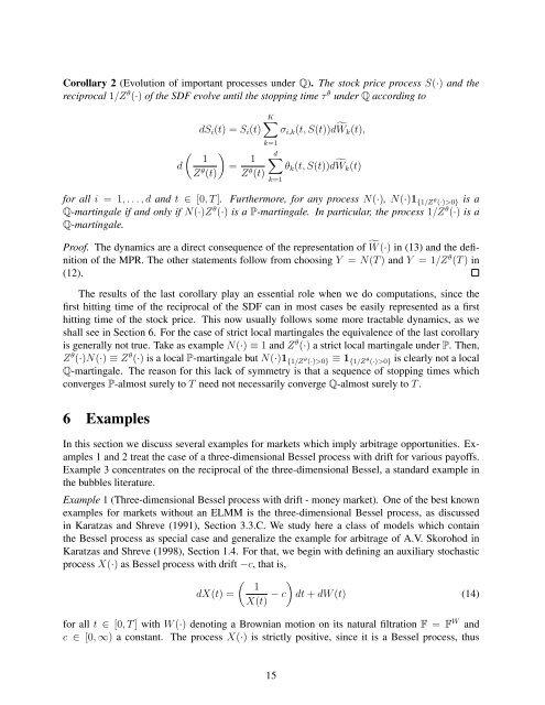
Corollary 2 (Evolution of important processes under Q). The stock price process S(·) and the
reciprocal 1/Z θ (·) of the SDF evolve until the stopping time τ θ under Q according to
dSi(t) = Si(t)
�
1
d
Zθ �
=
(t)
1
Zθ (t)
K�
σi,k(t, S(t))d� Wk(t),
k=1
d�
θk(t, S(t))d� Wk(t)
k=1
for all i = 1, . . . , d and t ∈ [0, T ]. Furthermore, for any process N(·), N(·)1 {1/Z θ (·)>0} is a
Q-martingale if and only if N(·)Z θ (·) is a P-martingale. In particular, the process 1/Z θ (·) is a
Q-martingale.
Proof. The dynamics are a direct consequence of the representation of � W (·) in (13) and the definition
of the MPR. The other statements follow from choosing Y = N(T ) and Y = 1/Z θ (T ) in
(12).
The results of the last corollary play an essential role when we do computations, since the
first hitting time of the reciprocal of the SDF can in most cases be easily represented as a first
hitting time of the stock price. This now usually follows some more tractable dynamics, as we
shall see in Section 6. For the case of strict local martingales the equivalence of the last corollary
is generally not true. Take as example N(·) ≡ 1 and Z θ (·) a strict local martingale under P. Then,
Z θ (·)N(·) ≡ Z θ (·) is a local P-martingale but N(·)1 {1/Z θ (·)>0} ≡ 1 {1/Z θ (·)>0} is clearly not a local
Q-martingale. The reason for this lack of symmetry is that a sequence of stopping times which
converges P-almost surely to T need not necessarily converge Q-almost surely to T .
6 Examples
In this section we discuss several examples for markets which imply arbitrage opportunities. Examples
1 and 2 treat the case of a three-dimensional Bessel process with drift for various payoffs.
Example 3 concentrates on the reciprocal of the three-dimensional Bessel, a standard example in
the bubbles literature.
Example 1 (Three-dimensional Bessel process with drift - money market). One of the best known
examples for markets without an ELMM is the three-dimensional Bessel process, as discussed
in Karatzas and Shreve (1991), Section 3.3.C. We study here a class of models which contain
the Bessel process as special case and generalize the example for arbitrage of A.V. Skorohod in
Karatzas and Shreve (1998), Section 1.4. For that, we begin with defining an auxiliary stochastic
process X(·) as Bessel process with drift −c, that is,
� �
1
dX(t) = − c dt + dW (t) (14)
X(t)
for all t ∈ [0, T ] with W (·) denoting a Brownian motion on its natural filtration F = F W and
c ∈ [0, ∞) a constant. The process X(·) is strictly positive, since it is a Bessel process, thus
15