Hedging under arbitrage

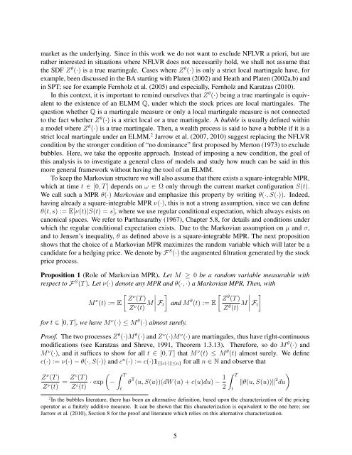
market as the underlying. Since in this work we do not want to exclude NFLVR a priori, but are
rather interested in situations where NFLVR does not necessarily hold, we shall not assume that
the SDF Z θ (·) is a true martingale. Cases where Z θ (·) is only a strict local martingale have, for
example, been discussed in the BA starting with Platen (2002) and Heath and Platen (2002a,b) and
in SPT; see for example Fernholz et al. (2005) and especially, Fernholz and Karatzas (2010).
In this context, it is important to remind ourselves that Z θ (·) being a true martingale is equivalent
to the existence of an ELMM Q, under which the stock prices are local martingales. The
question whether Q is a martingale measure or only a local martingale measure is not connected
to the fact whether Z θ (·) is a strict local or a true martingale. A bubble is usually defined within
a model where Z θ (·) is a true martingale. Then, a wealth process is said to have a bubble if it is a
strict local martingale under an ELMM. 2 Jarrow et al. (2007, 2010) suggest replacing the NFLVR
condition by the stronger condition of “no dominance” first proposed by Merton (1973) to exclude
bubbles. Here, we take the opposite approach. Instead of imposing a new condition, the goal of
this analysis is to investigate a general class of models and study how much can be said in this
more general framework without having the tool of an ELMM.
To keep the Markovian structure we will also assume that there exists a square-integrable MPR,
which at time t ∈ [0, T ] depends on ω ∈ Ω only through the current market configuration S(t).
We call such a MPR θ(·) Markovian and emphasize this property by writing θ(·, S(·)). Indeed,
having already a square-integrable MPR ν(·), this is not a strong assumption, since we can define
θ(t, s) := E[ν(t)|S(t) = s], where we use regular conditional expectation, which always exists on
canonical spaces. We refer to Parthasarathy (1967), Chapter 5.8, for details and conditions under
which the regular conditional expectation exists. Due to the Markovian assumption on µ and σ,
and to Jensen’s inequality, θ as defined above is a square-integrable MPR. The next proposition
shows that the choice of a Markovian MPR maximizes the random variable which will later be a
candidate for a hedging price. We denote by F S (·) the augmented filtration generated by the stock
price process.
Proposition 1 (Role of Markovian MPR). Let M ≥ 0 be a random variable measurable with
respect to F S (T ). Let ν(·) denote any MPR and θ(·, ·) a Markovian MPR. Then, with
M ν � ν Z (T )
(t) := E
Zν (t) M
�
�
�
� Ft
�
and M θ � θ Z (T )
(t) := E
Zθ (t) M
�
�
�
� Ft
�
for t ∈ [0, T ], we have M ν (·) ≤ M θ (·) almost surely.
Proof. The two processes Z θ (·)M θ (·) and Z ν (·)M ν (·) are martingales, thus have right-continuous
modifications (see Karatzas and Shreve, 1991, Theorem 1.3.13). Therefore, so do M θ (·) and
M ν (·), and it suffices to show for all t ∈ [0, T ] that M ν (t) ≤ M θ (t) almost surely. We define
c(·) := ν(·) − θ(·, S(·)) and c n (·) := c(·)1{�c(·)�≤n} for all n ∈ N and observe that
Zν (T )
Zν (t) = Zc (T )
Zc � � T
· exp − θ
(t) t
T (u, S(u))(dW (u) + c(u)du) − 1
� T
�θ(u, S(u))�
2 t
2 �
du
2 In the bubbles literature, there has been an alternative definition, based upon the characterization of the pricing
operator as a finitely additive measure. It can be shown that this characterization is equivalent to the one here; see
Jarrow et al. (2010), Section 8 for the proof and literature which relies on this alternative characterization.
5