Hedging under arbitrage

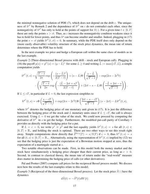
the minimal nonnegative solution of PDE (7), which does not depend on the drift c. The uniqueness
of hp0 by Remark 2 and the dependence of hp0 on c do not contradict each other, since the
nonnegativity of hp0 has only to hold at the points of support for S(·). For a given time t ∈ [0, T ]
these are only the points s > ct. Thus, as c increases the nonnegativity condition weakens since it
has to hold for fewer points, and thus hp can become smaller and smaller. Indeed, plugging in (17)
the point s = ct yields hp0(t, ct) = 0. In summary, while the PDE itself does only depend on the
(more easily observable) volatility structure of the stock price dynamics, the mean rate of return
determines where the PDE has to hold.
In the next example we price and hedge a European call within the same class of models as in
the last example.
Example 2 (Three-dimensional Bessel process with drift - stock and European call). Plugging in
(16) the payoff p(s) = pC (s) = (y − L) + for some L ≥ 0 and writing ˜ L := max{cT, L}, a simple
computation yields
� � �
� �
T − t
h pC
(t, s) =
s − ˜ L
√ T − t
2π exp − (s − ˜ L) 2
+ (s − L)Φ
− exp(2cs − 2c
2(T − t)
2 t)
��
T − t
·
2π exp
�
− (˜ L − 2ct + s) 2
�
�
−
+ (2ct − s − L)Φ
2(T − t)
˜ ��
L + 2ct − s
√ .
T − t
If L ≤ cT , in particular if L = 0, the last expression simplifies to
h pC
� �
s − cT
(t, s) = sΦ √ + exp(2cs − 2c
T − t
2 �
2ct − s − cT
t)Φ √
T − t
�
(s − 2ct) − Lh p0
(t, s),
where hp0 denotes the hedging price of one monetary unit given in (17). It is just the difference
between the hedging price of the stock and L monetary units since if L ≤ cT , the call is always
exercised. Using L = 0 we get the value of the stock. We could now proceed by computing the
derivative of hpC in s to get the hedge. Furthermore, the modified put-call parity of Corollary 1
provides us directly with the hedging price for a put.
If L = c = 0, we write p1 ≡ pL and the last equality yields hp1(t, s) = s for all (t, s) ∈
[0, T ] × R+ and holding the stock is optimal. There are two other ways to see this result right
away. Simple computations show directly that ˜ Zθ,t,s (T ) = s/S(T ) if c = 0, thus hp1(t, s) = s
for all (t, s) ∈ [0, T ] × R+. Alternatively, using the representation of hp1(t, s) implied by (12) we
see that the hedging price is just the expectation of a Brownian motion stopped at zero, thus the
expectation of a martingale started at s.
Two notable observations can be made. First, in this model both the money market and the
stock have simultaneously a hedging price cheaper than their current price, as long as c > 0.
Second, in contrast to classical theory, the mean rate of return under the “real-world” measure
does matter in determining the hedging price of calls (or other derivatives).
Pal and Protter (2007) compute call prices for the reciprocal Bessel process model. We discuss
next how the results of the last examples relate to this model.
Example 3 (Reciprocal of the three-dimensional Bessel process). Let the stock price ˜ S(·) have the
dynamics
d ˜ S(t) = − ˜ S 2 (t)dW (t)
17