Wetlands of Lassen Volcanic National Park - NPS Inventory and ...
Wetlands of Lassen Volcanic National Park - NPS Inventory and ...
Wetlands of Lassen Volcanic National Park - NPS Inventory and ...

You also want an ePaper? Increase the reach of your titles
YUMPU automatically turns print PDFs into web optimized ePapers that Google loves.
<strong>National</strong> <strong>Park</strong> Service<br />
U.S. Department <strong>of</strong> the Interior<br />
Natural Resource Program Center<br />
<strong>Wetl<strong>and</strong>s</strong> <strong>of</strong> <strong>Lassen</strong> <strong>Volcanic</strong> <strong>National</strong> <strong>Park</strong>:<br />
An Assessment <strong>of</strong> Vegetation, Ecological Services, <strong>and</strong><br />
Condition<br />
Natural Resource Technical Report <strong>NPS</strong>/KLMN/NRTR—2008/113
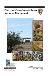
ON THE COVER<br />
A wetl<strong>and</strong> in <strong>Lassen</strong> <strong>Volcanic</strong> <strong>National</strong> <strong>Park</strong>.<br />
Photograph by: Cheryl Bartlett
<strong>Wetl<strong>and</strong>s</strong> <strong>of</strong> <strong>Lassen</strong> <strong>Volcanic</strong> <strong>National</strong> <strong>Park</strong>: An<br />
Assessment <strong>of</strong> Vegetation, Ecological Services, <strong>and</strong><br />
Condition<br />
Natural Resource Technical Report <strong>NPS</strong>/KLMN/NRTR—2008/113<br />
Paul R. Adamus, PhD<br />
College <strong>of</strong> Oceanic <strong>and</strong> Atmospheric Sciences<br />
Oregon State University<br />
104 COAS Administrative Bldg<br />
Corvallis, OR 973315503<br />
Cheryl L. Bartlett<br />
Department <strong>of</strong> Botany <strong>and</strong> Plant Pathology<br />
Oregon State University<br />
2082 Cordley Hall<br />
Corvallis, OR 973312902<br />
March 2008<br />
U.S. Department <strong>of</strong> the Interior<br />
<strong>National</strong> <strong>Park</strong> Service<br />
Natural Resource Program Center<br />
Fort Collins, Colorado
The Natural Resource Publication series addresses natural resource topics that are <strong>of</strong> interest <strong>and</strong><br />
applicability to a broad readership in the <strong>National</strong> <strong>Park</strong> Service <strong>and</strong> to others in the management<br />
<strong>of</strong> natural resources, including the scientific community, the public, <strong>and</strong> the <strong>NPS</strong> conservation<br />
<strong>and</strong> environmental constituencies. Manuscripts are peerreviewed to ensure that the information<br />
is scientifically credible, technically accurate, appropriately written for the intended audience,<br />
<strong>and</strong> is designed <strong>and</strong> published in a pr<strong>of</strong>essional manner.<br />
The Natural Resource Technical Reports series is used to disseminate the peerreviewed results<br />
<strong>of</strong> scientific studies in the physical, biological, <strong>and</strong> social sciences for both the advancement <strong>of</strong><br />
science <strong>and</strong> the achievement <strong>of</strong> the <strong>National</strong> <strong>Park</strong> Service’s mission. The reports provide<br />
contributors with a forum for displaying comprehensive data that are <strong>of</strong>ten deleted from journals<br />
because <strong>of</strong> page limitations. Current examples <strong>of</strong> such reports include the results <strong>of</strong> research that<br />
addresses natural resource management issues; natural resource inventory <strong>and</strong> monitoring<br />
activities; resource assessment reports; scientific literature reviews; <strong>and</strong> peer reviewed<br />
proceedings <strong>of</strong> technical workshops, conferences, or symposia.<br />
Views, statements, findings, conclusions, recommendations <strong>and</strong> data in this report are solely<br />
those <strong>of</strong> the author(s) <strong>and</strong> do not necessarily reflect views <strong>and</strong> policies <strong>of</strong> the U.S. Department <strong>of</strong><br />
the Interior, <strong>NPS</strong>. Mention <strong>of</strong> trade names or commercial products does not constitute<br />
endorsement or recommendation for use by the <strong>National</strong> <strong>Park</strong> Service.<br />
Printed copies <strong>of</strong> reports in these series may be produced in a limited quantity <strong>and</strong> they are only<br />
available as long as the supply lasts. This report is also available from the Natural Resource<br />
Publications Management website (http://www.nature.nps.gov/publications/NRPM) on the<br />
Internet or by sending a request to the address on the back cover.<br />
Please cite this publication as:<br />
Adamus, P. R., <strong>and</strong> C. L. Bartlett. 2008. <strong>Wetl<strong>and</strong>s</strong> <strong>of</strong> <strong>Lassen</strong> <strong>Volcanic</strong> <strong>National</strong> <strong>Park</strong>: An<br />
assessment <strong>of</strong> vegetation, ecological services, <strong>and</strong> condition. Natural Resource Technical Report<br />
<strong>NPS</strong>/KLMN/NRTR—2008/113. <strong>National</strong> <strong>Park</strong> Service, Fort Collins, Colorado.<br />
<strong>NPS</strong> D163, March 2008<br />
ii
Contents<br />
Page<br />
Appendixes.................................................................................................................................v<br />
Figures......................................................................................................................................vii<br />
Tables........................................................................................................................................ix<br />
Summary ...................................................................................................................................xi<br />
Acknowledgments ...................................................................................................................xiii<br />
1.0 Introduction ..........................................................................................................................1<br />
1.1 Study Background <strong>and</strong> Objectives...................................................................................1<br />
1.2 Wetl<strong>and</strong> Health <strong>and</strong> Its Indicators....................................................................................1<br />
1.3 General Description <strong>of</strong> LAVO...........................................................................................3<br />
1.4 Previous <strong>and</strong> Ongoing Studies Related to the <strong>Park</strong>’s <strong>Wetl<strong>and</strong>s</strong> ..........................................4<br />
2.0 Methods................................................................................................................................7<br />
2.1 Initial Site Characterization...............................................................................................7<br />
2.2 Wetl<strong>and</strong> <strong>Inventory</strong>.............................................................................................................7<br />
2.3 Field Site Selection ...........................................................................................................8<br />
2.4 Field Data Collection ...................................................................................................... 12<br />
2.5 Data Analysis.................................................................................................................. 14<br />
3.0 Results................................................................................................................................ 17<br />
3.1 Wetl<strong>and</strong> <strong>Inventory</strong>........................................................................................................... 17<br />
3.2 <strong>Wetl<strong>and</strong>s</strong> Pr<strong>of</strong>ile.............................................................................................................. 18<br />
3.3 Wetl<strong>and</strong> Health ............................................................................................................... 28<br />
3.4 Valued Ecological Services <strong>of</strong> <strong>Wetl<strong>and</strong>s</strong>: Estimates Based on Heuristic Models.............. 41<br />
4.0 Discussion .......................................................................................................................... 51<br />
4.1 Implications for <strong>Wetl<strong>and</strong>s</strong> Management in LAVO........................................................... 51<br />
4.2 Broader Applications ...................................................................................................... 52<br />
5.0 Literature Cited................................................................................................................... 55<br />
iii
Appendixes<br />
Page<br />
Appendix A. Data Dictionary Introduction................................................................................ 59<br />
Appendix B. Field Datasheets................................................................................................... 61<br />
Appendix C. Field Data Collection Protocols............................................................................ 77<br />
Appendix D. Wetl<strong>and</strong> Plant Species <strong>of</strong> LAVO, including Both Wetl<strong>and</strong> <strong>and</strong> Nonwetl<strong>and</strong> Species<br />
Found in LAVO <strong>Wetl<strong>and</strong>s</strong> in 2005............................................................................................ 81<br />
Appendix E. Plant Metrics for Individual Visited <strong>Wetl<strong>and</strong>s</strong> ...................................................... 93<br />
Appendix F. CRAM Scores <strong>and</strong> Ecological Service Ratings <strong>of</strong> Visited LAVO <strong>Wetl<strong>and</strong>s</strong>.......... 99<br />
Appendix G. Amphibians, Reptiles, Fish, <strong>and</strong> Fairy Shrimp Noted in or near LAVO <strong>Wetl<strong>and</strong>s</strong> by<br />
this Study or Stead et al. (2005) .............................................................................................. 103<br />
Appendix H. Bird Species Regularly Present in Summer in LAVO <strong>and</strong> That Are Associated<br />
Strongly with <strong>Wetl<strong>and</strong>s</strong> <strong>and</strong> Water Bodies .............................................................................. 105<br />
Appendix I. Mammals <strong>of</strong> LAVO That Are Probably the Most Dependent on <strong>Wetl<strong>and</strong>s</strong> <strong>and</strong> Water<br />
Bodies .................................................................................................................................... 107<br />
Appendix J. Photographs <strong>of</strong> the Defined Wetl<strong>and</strong> Plant Communities..................................... 109<br />
v
Figures<br />
Page<br />
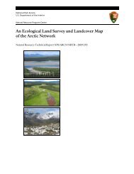
Figure 1. The rugged highelevation l<strong>and</strong>scape <strong>of</strong> <strong>Lassen</strong> <strong>Volcanic</strong> <strong>National</strong> <strong>Park</strong>. .................. xiii<br />
Figure 2. Groundwaterfed wetl<strong>and</strong>s in LAVO <strong>of</strong>ten occur in meadows at the toe <strong>of</strong> steep slopes.<br />
....................................................................................................................................................2<br />
Figure 3. Wetl<strong>and</strong> on the fringe <strong>of</strong> a pond. ...................................................................................5<br />
Figure 4. Map <strong>of</strong> LAVO wetl<strong>and</strong>s visited <strong>and</strong> assessed during 2005. .........................................10<br />
Figure 5. Assessing soils in a LAVO wetl<strong>and</strong>. ...........................................................................13<br />
Figure 6. Site NR342, a probable acid geothermal fen. Note the pool morphology <strong>and</strong> abundant<br />
Sphagnum moss that are typical. ................................................................................................24<br />
Figure 7. Bumpass Hell acid geothermal fen. Bumpass Hell is just below the exposed whitish<br />
hillside in the background <strong>of</strong> the photo; the large pool at the terminus <strong>of</strong> the wetl<strong>and</strong> can be seen<br />
in immediately in front <strong>of</strong> that hillside. ......................................................................................25<br />
Figure 8. Wetl<strong>and</strong> vegetation along shoreline that has been impacted by excessive <strong>of</strong>ftrail foot<br />
traffic.........................................................................................................................................29<br />
Figure 9. Remnants <strong>of</strong> more intensive l<strong>and</strong> uses during historic times in LAVO. .......................30<br />
Figure 10. Site frequency distribution for wetl<strong>and</strong>associated plant species <strong>of</strong> LAVO. ...............34<br />
Figure 11. Plant speciesarea relationship among all wetl<strong>and</strong>s surveyed in LAVO. ....................35<br />
Figure 12. Statistically significant relationship in LAVO wetl<strong>and</strong>s between proportion <strong>of</strong> species<br />
that are disturbance species <strong>and</strong> wetl<strong>and</strong> distance from a road....................................................37<br />
Figure 13. Note the b<strong>and</strong>s on the rock in the foreground, indicating changing water levels which<br />
are evidence <strong>of</strong> water being stored seasonally in this LAVO wetl<strong>and</strong>. ........................................43<br />
Figure 14. Upturned trees (right) are a sign <strong>of</strong> increasing water levels in some wetl<strong>and</strong>s; the<br />
resulting pools create habitat for aquatic invertebrates <strong>and</strong> amphibians. .....................................46<br />
Figure 15. Large pieces <strong>of</strong> downed wood provide essential habitat for many LAVO wildlife<br />
species. ......................................................................................................................................47<br />
vii
Tables<br />
Page<br />
Table 1. Summary <strong>of</strong> past water quality exceedences in LAVO water bodies...............................6<br />
Table 2. GPS coordinates <strong>and</strong> general descriptive information on the assessed wetl<strong>and</strong>s. ...........11<br />
Table 3. Number <strong>and</strong> area <strong>of</strong> LAVO wetl<strong>and</strong>s by hydrogeomorphic (HGM) class, as estimated<br />
using two methods (comprehensive GISbased vs. fieldchecked sites). .....................................18<br />
Table 4. Number <strong>and</strong> area <strong>of</strong> LAVO wetl<strong>and</strong>s summarized by Cowardin classification shown on<br />
NWI maps. ................................................................................................................................19<br />
Table 5. Preliminary vegetationbased wetl<strong>and</strong> communities <strong>of</strong> LAVO derived by statistical<br />
processing <strong>of</strong> data from 78 wetl<strong>and</strong> plots. ..................................................................................21<br />
Table 6. Botanical metrics for herb plots, by community class. ..................................................23<br />
Table 7. Statistical summaries for LAVO wetl<strong>and</strong> polygons as derived from existing geospatial<br />
data. The first number in each vertical pair is for the wetl<strong>and</strong>s in our statistical sample, the second<br />
is for all LAVO wetl<strong>and</strong>s mapped by the NWI...........................................................................27<br />
Table 8. Statistical summaries for LAVO wetl<strong>and</strong> polygons as derived from existing geospatial<br />
data. The first number in each vertical pair is for the wetl<strong>and</strong>s in our statistical sample, the second<br />
is for all LAVO wetl<strong>and</strong>s mapped by the NWI (continued). .......................................................28<br />
Table 9. Frequency <strong>of</strong> artificial features noted in or near LAVO wetl<strong>and</strong>s..................................28<br />
Table 10. Artificial features found in visited wetl<strong>and</strong>s................................................................29<br />
Table 11. Survey effectiveness for detecting wetl<strong>and</strong> indicator plant species known to occur in<br />
LAVO. ......................................................................................................................................33<br />
Table 12. Statistical summaries <strong>of</strong> botanical metrics for pooled polygon <strong>and</strong> plot data. ..............38<br />
Table 13. Statistical summaries <strong>of</strong> botanical metrics at plot scale (herb plots only). ...................38<br />
Table 14. Statistical summaries, by HGM class, <strong>of</strong> botanical metrics at plot scale. .....................39<br />
Table 15. Statistical summaries <strong>of</strong> botanical metrics at plot scale (shrub/forest plots only).........39<br />
Table 16. CRAM scores from visited LAVO wetl<strong>and</strong>s: summary statistics. ...............................40<br />
Table 17. Health assessment <strong>of</strong> visited LAVO wetl<strong>and</strong>s based on the draft Fen Condition<br />
Checklist....................................................................................................................................41<br />
Table 18. Model for describing relative capacity <strong>of</strong> LAVO wetl<strong>and</strong>s for natural water storage <strong>and</strong><br />
slowing <strong>of</strong> infiltration. ...............................................................................................................42<br />
Table 19. Model for describing relative capacity <strong>of</strong> LAVO wetl<strong>and</strong>s for intercepting <strong>and</strong><br />
stabilizing suspended sediments.................................................................................................43<br />
Table 20. Model for describing relative capacity <strong>of</strong> LAVO wetl<strong>and</strong>s for processing nutrients,<br />
metals, <strong>and</strong> other substances. .....................................................................................................44<br />
Table 21. Model for describing relative capacity <strong>of</strong> LAVO wetl<strong>and</strong>s for sequestering carbon. ...44<br />
Table 22. Model for describing relative capacity <strong>of</strong> LAVO wetl<strong>and</strong>s for maintaining surface<br />
water temperatures.....................................................................................................................45<br />
Table 23. Model for describing relative capacity <strong>of</strong> LAVO wetl<strong>and</strong>s for supporting native<br />
invertebrate diversity. ................................................................................................................45<br />
Table 24. Model for describing relative capacity <strong>of</strong> LAVO wetl<strong>and</strong>s for supporting native fish..46<br />
Table 25. Model for describing the relative capacity <strong>of</strong> LAVO wetl<strong>and</strong>s for supporting native<br />
amphibians <strong>and</strong> reptiles..............................................................................................................47<br />
Table 26. Model for describing the relative capacity <strong>of</strong> LAVO wetl<strong>and</strong>s for supporting native<br />
birds <strong>and</strong> mammals. ...................................................................................................................48<br />
Table 27. Number (percent) <strong>of</strong> wetl<strong>and</strong>s capable <strong>of</strong> performing selected ecological services, for<br />
just the visited wetl<strong>and</strong>s that comprised the statistical sample. ...................................................48<br />
ix
Table 28. Normative ranges for ecological service <strong>and</strong> health metrics in wetl<strong>and</strong>s <strong>of</strong> LAVO (all<br />
HGM classes combined). ...........................................................................................................54<br />
x
Summary<br />
During 2005, we visited <strong>and</strong> assessed the health <strong>of</strong> 68 wetl<strong>and</strong>s throughout <strong>Lassen</strong> <strong>Volcanic</strong> <strong>National</strong><br />
<strong>Park</strong> (LAVO), covering an area equal to 39% <strong>of</strong> the park’s wetl<strong>and</strong> area. Of the wetl<strong>and</strong>s visited, 47<br />
were selected using a statistical procedure that drew a spatiallybalanced r<strong>and</strong>omized sample from an<br />
existing map <strong>of</strong> LAVO wetl<strong>and</strong>s. Among the visited wetl<strong>and</strong>s, we surveyed a total <strong>of</strong> 78 plots<br />
dominated by herbaceous wetl<strong>and</strong> vegetation <strong>and</strong> 15 plots dominated by wetl<strong>and</strong> shrubs or trees. We<br />
also characterized soil pr<strong>of</strong>iles <strong>and</strong> observed hydrologic conditions. Before beginning the field work,<br />
we used GIS <strong>and</strong> a variety <strong>of</strong> existing spatial data layers to quantitatively characterize all mapped<br />
LAVO wetl<strong>and</strong>s.<br />
<strong>Wetl<strong>and</strong>s</strong> in LAVO occur in a variety <strong>of</strong> settings, including stream riparian areas, pond margins, alder<br />
covered slopes, springs, montane meadows, <strong>and</strong> snowmelt depressions. Based on the hydrogeomorphic<br />
(HGM) classification system, about 45% <strong>of</strong> the wetl<strong>and</strong>s are Depressions or Flats, 38% are Slope<br />
wetl<strong>and</strong>s, 7% are Riverine, <strong>and</strong> 1% are Lacustrine Fringe. Based on the Cowardin classification<br />
system, 34% <strong>of</strong> the LAVO wetl<strong>and</strong>s area is emergent vegetation, 24% is scrubshrub, 7% is forested,<br />
<strong>and</strong> the remainder is open water or aquatic bed. Slightly fewer than onethird <strong>of</strong> the wetl<strong>and</strong>s retain<br />
some surface water yearround. At least one plant species characteristic <strong>of</strong> fens (an uncommon type <strong>of</strong><br />
mossy groundwaterfed wetl<strong>and</strong>) was found in 23 <strong>of</strong> the wetl<strong>and</strong>s, but soil pr<strong>of</strong>iles provided definitive<br />
evidence <strong>of</strong> fen conditions in only two <strong>of</strong> the visited wetl<strong>and</strong>s. We discovered three wetl<strong>and</strong>s that<br />
appear to be a type – acid geothermal fen – that is rare globally <strong>and</strong> apparently had not been<br />
documented previously in the SierraCascade system.<br />
Many factors define wetl<strong>and</strong> health (or integrity), including contaminants in air, soil, vegetation, <strong>and</strong><br />
water that were not measured by this study. Few indicators <strong>of</strong> wetl<strong>and</strong> health can be estimated rapidly<br />
<strong>and</strong> at reasonable cost across a large number <strong>of</strong> wetl<strong>and</strong>s. When health is defined solely by the<br />
prevalence <strong>of</strong> native plant species <strong>and</strong> scores from the California Rapid Assessment Method (CRAM),<br />
most LAVO wetl<strong>and</strong>s appear to be relatively healthy. We found 19 disturbanceassociated plant<br />
species (6% <strong>of</strong> all species we encountered) among 44 <strong>of</strong> the 68 wetl<strong>and</strong>s we visited. From zero to six<br />
such species were found per wetl<strong>and</strong>, but never dominated the vegetation cover. They were more<br />
frequent near roads but not trails.<br />
Our sample <strong>of</strong> just 68 wetl<strong>and</strong>s detected 51% <strong>of</strong> LAVO’s known wetl<strong>and</strong> flora, <strong>and</strong> added six species<br />
to the LAVO plant list. Among the 338 plant taxa (both wetl<strong>and</strong> <strong>and</strong> upl<strong>and</strong>) we found in the visited<br />
wetl<strong>and</strong>s were at least two that are listed by the California Native Plant Society as rare or having<br />
limited distribution. In most wetl<strong>and</strong>s, more than 30 plant species were found, <strong>and</strong> most <strong>of</strong> the 100 m 2<br />
herbaceous plots we surveyed had more than 13, with a maximum <strong>of</strong> 43. The plant species<br />
composition tended to be more unique in wetl<strong>and</strong>s that were dominated by emergent (herbaceous)<br />
vegetation, not on lakeshores, at lower elevations, <strong>and</strong> intercepted by streams.<br />
<strong>Wetl<strong>and</strong>s</strong> in LAVO perform a variety <strong>of</strong> ecological services. In each visited wetl<strong>and</strong>, we visually<br />
assessed presumed indicators <strong>of</strong> nine <strong>of</strong> the most common ecological services (functions). Based on<br />
that, we found that more <strong>of</strong> LAVO’s wetl<strong>and</strong>s are likely to support native invertebrates, birds, <strong>and</strong><br />
mammals at a high capacity than are likely to effectively support fish, filter suspended sediments, or<br />
maintain surface water temperatures.<br />
xi
Although major objectives <strong>of</strong> this project did not include mapping wetl<strong>and</strong> boundaries or<br />
comprehensively identifying previously unmapped wetl<strong>and</strong>s, we did incidentally discover 87<br />
unmapped wetl<strong>and</strong>s <strong>and</strong> found that the spatial extent <strong>of</strong> many mapped wetl<strong>and</strong>s had been<br />
underestimated. All visited sites that had been previously mapped as wetl<strong>and</strong>s were found by our field<br />
inspection to be wetl<strong>and</strong>s. Attempts to develop spatial models for predicting occurrence <strong>of</strong> unmapped<br />
wetl<strong>and</strong>s were only partially successful, due mainly to limitations <strong>of</strong> existing spatial data layers.<br />
xii
Acknowledgments<br />
The need for this project was identified by Dr. Daniel Sarr, I & M Coordinator, Klamath Network,<br />
<strong>National</strong> <strong>Park</strong> Service. His support <strong>and</strong> feedback throughout the project was absolutely crucial to its<br />
success. Dr. Jim Good at Oregon State University administered the agreement (Cooperative Agreement<br />
#CA9088A0008). At <strong>Lassen</strong> <strong>Volcanic</strong> <strong>National</strong> <strong>Park</strong> (Figure 1), the thoughtful administrative support<br />
from Nancy Nordensten (Biologist) <strong>and</strong> Louise Johnson (Chief <strong>of</strong> Resources Management) helped our<br />
field work go smoothly. Field assessments <strong>of</strong> wetl<strong>and</strong> soils were done by Nick Pacini, <strong>and</strong> John<br />
Beickel helped with a variety <strong>of</strong> field tasks. Early in the project, Andrew Duff (then at Southern<br />
Oregon University) used GIS to identify <strong>and</strong> compile the most important spatial data layers for LAVO.<br />
Expert assistance with identification <strong>of</strong> sedges was provided by Dr. Laurence Janeway at Chico State<br />
University. Dr. David Cooper <strong>of</strong> Colorado State University generously shared his knowledge <strong>of</strong> Sierra<br />
fens. Jennifer Larsen <strong>and</strong> Rebecca Tully, graduate students advised by the author at Oregon State<br />
University, assisted with the GIS tasks <strong>and</strong> data entry tasks, respectively.<br />
Figure 1. The rugged highelevation l<strong>and</strong>scape <strong>of</strong> <strong>Lassen</strong> <strong>Volcanic</strong> <strong>National</strong> <strong>Park</strong>.<br />
xiii
1.0 Introduction<br />
1.1 Study Background <strong>and</strong> Objectives<br />
<strong>Wetl<strong>and</strong>s</strong> include portions <strong>of</strong> features as varied as springs, seeps, alder swales, montane meadows,<br />
cottonwood st<strong>and</strong>s, ponds, beaver impoundments, snowmelt pools, marshes, bogs, <strong>and</strong> fens. As water<br />
gathering foci in watersheds, wetl<strong>and</strong>s are especially vulnerable to impacts at l<strong>and</strong>scape <strong>and</strong> local<br />
scales. They also are an excellent indicator <strong>of</strong> the overall ecological health <strong>of</strong> the watersheds within<br />
which they occur. <strong>Wetl<strong>and</strong>s</strong> in <strong>Lassen</strong> <strong>Volcanic</strong> <strong>National</strong> <strong>Park</strong> (LAVO) are potentially vulnerable to a<br />
range <strong>of</strong> cumulative impacts, including nonnative species invasions, airborne or waterborne<br />
pollutants, hydrologic alterations, <strong>and</strong> excessive traffic. Some <strong>of</strong> them may be experiencing lingering<br />
effects <strong>of</strong> grazing, drainage, <strong>and</strong> logging that occurred historically, as well as the volcanic eruptions <strong>of</strong><br />
19141915.<br />
Like a similar project in Crater Lake <strong>National</strong> <strong>Park</strong> (Adamus <strong>and</strong> Bartlett 2008), this project sought to<br />
address three main questions:<br />
• What is the general accuracy <strong>of</strong> the existing <strong>National</strong> <strong>Wetl<strong>and</strong>s</strong> <strong>Inventory</strong> (NWI) maps <strong>of</strong><br />
LAVO wetl<strong>and</strong>s?<br />
• What is the relative ecological health <strong>of</strong> LAVO wetl<strong>and</strong>s?<br />
• What is the most consistent <strong>and</strong> logical scheme for defining plant species assemblages<br />
(communities) <strong>of</strong> LAVO wetl<strong>and</strong>s?<br />
These objectives are consistent with the park enabling legislation, the national goals <strong>of</strong> the <strong>Inventory</strong><br />
<strong>and</strong> Monitoring Program (including Vital Signs Monitoring), <strong>and</strong> future park management. This<br />
project was not intended to be either a research study (in the sense <strong>of</strong> testing specific hypotheses) or a<br />
comprehensive resource inventory <strong>of</strong> wetl<strong>and</strong>s or plant species. Rather, it is a resource assessment,<br />
characterizing the overall distribution, health, ecological services, <strong>and</strong> types <strong>of</strong> wetl<strong>and</strong>s within the<br />
park. Such an assessment is necessary to provide a baseline against which future changes may be<br />
monitored – <strong>and</strong> their causes sought <strong>and</strong> where necessary, remedied (Bedford 1996). Data compiled<br />
<strong>and</strong> analyzed by this assessment also support quantitative reference st<strong>and</strong>ards for ongoing wetl<strong>and</strong><br />
management <strong>and</strong> restoration activities. Currently, managers are hindered in assessing the severity <strong>of</strong><br />
possible impacts to wetl<strong>and</strong>s because there are no systematic data that quantify what unaltered<br />
wetl<strong>and</strong>s <strong>of</strong> each major type “should” look like, in terms <strong>of</strong> the range <strong>of</strong> plant diversity, species<br />
composition, <strong>and</strong> ecological services.<br />
1.2 Wetl<strong>and</strong> Health <strong>and</strong> Its Indicators<br />
Whether discussing wetl<strong>and</strong>s (Figure 2), forests, or rangel<strong>and</strong>s, the terms, “ecological condition,”<br />
“health,” “integrity,” <strong>and</strong> “quality” are <strong>of</strong>ten used interchangeably. As noted above, a major objective<br />
<strong>of</strong> this project was to estimate the proportion <strong>of</strong> LAVO wetl<strong>and</strong>s that are “healthy.” However, although<br />
scientists <strong>and</strong> policy makers have long struggled with the question <strong>of</strong> how to define wetl<strong>and</strong> health or<br />
ecological condition, no consensus on a definition <strong>of</strong> wetl<strong>and</strong> health – let alone an accepted procedure<br />
for measuring it comprehensively – currently exists (Young <strong>and</strong> Sanzone 2002). To some, health is<br />
synonymous with the “naturalness” <strong>of</strong> a wetl<strong>and</strong>’s biological communities <strong>and</strong> hydrologic regime. For<br />
example, by such criteria, wetl<strong>and</strong>s that support only native species, <strong>and</strong> especially native species that<br />
are intolerant <strong>of</strong> pollution <strong>and</strong> other human disturbance, are considered to be the healthiest. To other<br />
1
scientists <strong>and</strong> policy makers, wetl<strong>and</strong> health means the degree to which a wetl<strong>and</strong> performs various<br />
ecological services – such as storing water, retaining sediments, <strong>and</strong> providing habitat. Still other<br />
pr<strong>of</strong>essionals believe that wetl<strong>and</strong> health should reflect not only the performance <strong>of</strong> these ecological<br />
services (sometimes called “functions”), but also the value <strong>of</strong> the services that are provided to society<br />
in specific local settings. These three perspectives are not synonymous, interchangeable, or inevitably<br />
correlated, at least not when using only data that can be assessed rapidly (Hruby 1997, 1999, 2001).<br />
Alternatively, some have suggested use <strong>of</strong> the phrase, “proper functioning condition” to describe<br />
ecosystem health <strong>and</strong> have suggested qualitative indicators <strong>and</strong> a “condition checklist” for its<br />
assessment in fen wetl<strong>and</strong>s (see below) <strong>and</strong> freshwater wetl<strong>and</strong>s <strong>of</strong> the arid West (Pritchard 1994,<br />
Rocchio 2005). However, such checklists or scorecards require considerable judgment on the part <strong>of</strong><br />
the user, tend not to generate consistent results among users <strong>and</strong> across a variety <strong>of</strong> wetl<strong>and</strong> types in<br />
different regions, <strong>and</strong> are <strong>of</strong>ten not sensitive to important differences between wetl<strong>and</strong>s. The visually<br />
based estimates they provide have seldom been tested for correlation with meaningful measured data.<br />
Finally, the term “desired future condition” has been suggested. Although this term makes explicit the<br />
value judgments involved, the term can be defined by managers in almost any manner, which<br />
confounds the interpretation <strong>of</strong> results from broadscale comparative assessments.<br />
Figure 2. Groundwaterfed wetl<strong>and</strong>s in LAVO <strong>of</strong>ten occur in meadows at the toe <strong>of</strong> steep slopes.<br />
Attempts to define wetl<strong>and</strong> health become further confused when the simple presence <strong>of</strong> activities or<br />
features that have the potential to disturb wetl<strong>and</strong> biological communities, ecological services, <strong>and</strong><br />
values are assumed without sitespecific evidence to have had that effect, <strong>and</strong> the alteration is assumed<br />
2
to inevitably be “negative” from a human perspective. For example, a trail adjoining a small, sensitive<br />
wetl<strong>and</strong> has the potential to introduce sediment into the wetl<strong>and</strong> during periods <strong>of</strong> high run<strong>of</strong>f. But<br />
without further evidence, this cannot be assumed to occur, because many trails are on soils highly<br />
resistant to erosion. Even if sediment enters the wetl<strong>and</strong>, the effect on wetl<strong>and</strong> services, values, <strong>and</strong><br />
health cannot be assumed to necessarily be negative.<br />
A major challenge has always been to find indicators <strong>of</strong> the key ecological attributes <strong>and</strong> processes –<br />
as well as for wetl<strong>and</strong> health, ecological condition, naturalness, ecological services, <strong>and</strong> value – that<br />
are both highly repeatable (among different users) <strong>and</strong> practical to apply. Many features that could<br />
yield the most information for judging ecological services <strong>and</strong> health cannot be measured without a<br />
considerable monitoring investment in each wetl<strong>and</strong> over long periods <strong>of</strong> time. Examples include the<br />
duration <strong>and</strong> frequency <strong>of</strong> flooding, proportionate contributions <strong>of</strong> various sources <strong>of</strong> water, soil<br />
organic content <strong>and</strong> buildup rates, functional diversity <strong>of</strong> microbes <strong>and</strong> invertebrates, contamination <strong>of</strong><br />
sediments, seed germination rates, <strong>and</strong> wildlife productivity <strong>and</strong> consistency <strong>of</strong> use. Often the most<br />
rapid <strong>and</strong> objective (but not comprehensive) approach for estimating the health <strong>of</strong> wetl<strong>and</strong>s is to<br />
identify their plants. Many plant species can serve as excellent indicators <strong>of</strong> wetl<strong>and</strong> health (Adamus<br />
<strong>and</strong> Br<strong>and</strong>t 1990, Adamus et al. 2001); see also: http://www.epa.gov/waterscience/criteria/wetl<strong>and</strong>s/.<br />
In some regions, a “floristic quality index” has been developed <strong>and</strong> applied to assess wetl<strong>and</strong> health,<br />
but such a metric has not been developed for this region. It requires a considerable amount <strong>of</strong> basic<br />
information on tolerances <strong>of</strong> wetl<strong>and</strong> species to various types <strong>of</strong> disturbances.<br />
1.3 General Description <strong>of</strong> LAVO<br />
The following is paraphrased from existing LAVO reports by the <strong>NPS</strong>:<br />
Water Bodies <strong>and</strong> Alterations. The 106,372acre park contains over 200 lakes <strong>and</strong> ponds <strong>and</strong><br />
15 perennial streams. Some lakes have been significantly modified by stocking <strong>of</strong> nonnative<br />
sport fish, a practice that ended in 1980. Some <strong>of</strong> the natural drainage systems in the park have<br />
been altered. The most obvious <strong>of</strong> these are Manzanita <strong>and</strong> Reflection Lakes in the park’s<br />
northwest corner, <strong>and</strong> Dream Lake in Warner Valley. Manzanita Lake was created from the<br />
Chaos Crags rockfall avalanche 300 years ago <strong>and</strong> was enlarged with a dam in 1911 for a small<br />
hydropower operation. Water was also diverted from Manzanita Creek to Reflection Lake,<br />
originally a closed basin lake, to provide water power <strong>and</strong> to improve fish production. Dream<br />
Lake was impounded as a recreational <strong>and</strong> scenic feature for the Drakesbad resort. Natural<br />
drainage patterns in Warner Valley were also altered by early ranchers to more evenly<br />
distribute water in the meadow for livestock grazing. The park contains 42 miles <strong>of</strong> paved<br />
roads, 15 miles <strong>of</strong> unpaved roads, five small bridges, <strong>and</strong> 146 miles <strong>of</strong> trails.<br />
Soils. The soils are generally rocky, shallow, rapidly drained <strong>and</strong> strongly acidic. They are<br />
almost exclusively volcanic in origin. Depths vary from several feet in limited lower elevation<br />
meadows to thin or nonexistent on the higher elevations.<br />
Vegetation. As a result <strong>of</strong> the park being located near the junction <strong>of</strong> two great mountain<br />
ranges, the Cascades <strong>and</strong> the Sierra Nevada, <strong>and</strong> intersecting with the Great Basin, there is an<br />
overlap <strong>of</strong> floral species commonly specific to one <strong>of</strong> these provinces. The diversity <strong>of</strong> geologic<br />
formations <strong>and</strong> chemical <strong>and</strong> textural compositions <strong>of</strong> lava have resulted in a wide diversity <strong>of</strong><br />
plants in these communities <strong>and</strong> many anomalies to the altitudinal life zones. Four major plant<br />
communities are found within the park: yellow pine forest, red fir forest, subalpine forest, <strong>and</strong><br />
3
alpine fell fields. These correspond roughly to the four life zones: Transition, Canadian,<br />
Hudsonian, <strong>and</strong> Arcticalpine. The yellow pine forest, found at elevations below 6,000 feet,<br />
typically consists <strong>of</strong> sugar pine, Jeffrey pine, white fir, <strong>and</strong> incense cedar. The widespread red<br />
fir forests at elevations between 6,000 <strong>and</strong> 8,500 feet consist <strong>of</strong> lodgepole pine, Jeffrey pine,<br />
western white pine, red fir <strong>and</strong> mountain hemlock. The subalpine forest, at the upper limit <strong>of</strong><br />
the coniferous forest, is characterized by the whitebark pine, a highly weatherresistant plant<br />
that grows at elevations as high as 10,000 feet. Above timberline are the alpine meadows <strong>and</strong><br />
fell fields. Brushl<strong>and</strong> covers approximately 10% <strong>of</strong> the park, consisting primarily <strong>of</strong> greenleaf<br />
manzanita, pinemat manzanita, <strong>and</strong> snowbrush ceanothus. Other common shrubs are currant,<br />
gooseberry, serviceberry, bitter cherry, <strong>and</strong> California chinquapin. Much <strong>of</strong> the park is rocky,<br />
exposed, <strong>and</strong> relatively devoid <strong>of</strong> forest vegetation. <strong>Volcanic</strong> eruptions <strong>of</strong> <strong>Lassen</strong> Peak in 1914<br />
to 1915 destroyed over 7 square miles <strong>of</strong> forestl<strong>and</strong>. Pioneering lodgepole pines are now<br />
succeeding in many areas to the other pines <strong>and</strong> firs. Historically, human activities within the<br />
park included the grazing <strong>of</strong> horses, sheep, <strong>and</strong> cattle; the treatment <strong>of</strong> insectinfected trees; <strong>and</strong><br />
the suppression <strong>of</strong> virtually every wildfire for almost 90 years.<br />
1.4 Previous <strong>and</strong> Ongoing Studies Related to the <strong>Park</strong>’s <strong>Wetl<strong>and</strong>s</strong><br />
<strong>Wetl<strong>and</strong>s</strong> <strong>of</strong> LAVO have not previously been studied in a holistic <strong>and</strong> statisticallyrigorous manner.<br />
Botanists had previously visited many <strong>of</strong> the park’s wetl<strong>and</strong>s (as well as all other habitat types) non<br />
systematically, as reflected in publications on the park’s vascular plants (Gillett et al. 1961) <strong>and</strong><br />
mosses (Showers 1982). Their published data are <strong>of</strong> limited use in assessing wetl<strong>and</strong> health because<br />
they were not referenced to precise geographic locations. One large, partiallyrestored wetl<strong>and</strong> along<br />
the southern edge <strong>of</strong> the park – Drakesbad Meadow – has been the object <strong>of</strong> an intensive study <strong>of</strong> its<br />
hydrology, soils, <strong>and</strong> vegetation (Patterson 2005). Lichens have been monitored systematically since<br />
1996 along transects in nearby <strong>Lassen</strong> <strong>National</strong> Forest, as indicators <strong>of</strong> air quality. Although not<br />
specific to wetl<strong>and</strong>s, <strong>NPS</strong>sponsored efforts are currently underway to develop <strong>and</strong> apply a<br />
classification scheme to vegetation <strong>of</strong> LAVO <strong>and</strong> other parks in the region, building upon an earlier<br />
effort by White et al. (1995).<br />
Amphibians, reptiles, <strong>and</strong> fish were the objects <strong>of</strong> a rapid visual survey <strong>of</strong> 365 LAVO ponds (Figure<br />
3), lakes, <strong>and</strong> meadows in 2004 by researchers from the USDA Forest Service (Dr. Hartwell Welsh)<br />
<strong>and</strong> Southern Oregon University (Dr. Michael <strong>Park</strong>er) (Stead et al. 2005). Habitat characteristics <strong>of</strong><br />
those sites were also rapidly assessed, <strong>and</strong> all data were geographically referenced. For the present<br />
study, we surveyed plants, soils, <strong>and</strong> structural indicators <strong>of</strong> wetl<strong>and</strong> ecological services at many <strong>of</strong> the<br />
same sites. Also, park biologists <strong>and</strong> interns have surveyed some ponds <strong>and</strong> wetl<strong>and</strong>s for particular<br />
wildlife species, such as nesting bufflehead (a duck species that reaches the southern limit <strong>of</strong> its<br />
breeding range near the park). Invertebrate samples were collected in 2004 from many LAVO ponds<br />
<strong>and</strong> wetl<strong>and</strong>s, <strong>and</strong> a report summarizing the data has been prepared by Dr. Michael <strong>Park</strong>er <strong>of</strong> Southern<br />
Oregon University.<br />
Information on the distribution <strong>of</strong> soil types within the park is limited, but a comprehensive survey is<br />
currently underway. Water quality has been measured in various streams, lakes, <strong>and</strong> in a few springs,<br />
but not from wetl<strong>and</strong>s (<strong>NPS</strong>WRD 1999). Some <strong>of</strong> the results are summarized in Table 1. Water<br />
quality in wetl<strong>and</strong>s is determined not only by proximity to pollutantgenerating human activities, but<br />
also by water source (groundwater vs. surface water run<strong>of</strong>f), residence time (flow rate), location (high<br />
or low in watershed <strong>and</strong> east or west side <strong>of</strong> park, which correlate with precipitation), <strong>and</strong> soil type.<br />
4
Microbial <strong>and</strong> algal diversity in LAVO hot springs also has been characterized (e.g., Brown <strong>and</strong> Wolfe<br />
2006).<br />
Figure 3. Wetl<strong>and</strong> on the fringe <strong>of</strong> a pond.<br />
Outside the park, several publications discuss the ecological condition <strong>and</strong> threats to wetl<strong>and</strong>s <strong>and</strong><br />
other aquatic habitats in the northern Sierra – southern Cascade region (e.g., Moyle <strong>and</strong> R<strong>and</strong>all 1998).<br />
Quaking aspen st<strong>and</strong>s <strong>and</strong> montane meadows <strong>of</strong> the Sierras, many <strong>of</strong> which are wetl<strong>and</strong>s, are the focus<br />
<strong>of</strong> a regional wildlife <strong>and</strong> vegetation study by Dr. Mike Morrison <strong>and</strong> others from UC Davis. A<br />
statistical classification <strong>of</strong> vegetation communities <strong>of</strong> one <strong>of</strong> the region’s montane wetl<strong>and</strong> types – fens<br />
– was published recently by Cooper <strong>and</strong> Wolf (2006) <strong>and</strong> a vegetation classification has been<br />
attempted for the region’s riparian areas (Smith 1998). A qualitative method for assessing the<br />
ecological condition <strong>of</strong> fen wetl<strong>and</strong>s <strong>of</strong> the Sierras <strong>and</strong> southern Cascades was proposed by Weixelman<br />
et al. (2007), following generally the “Proper Functioning Condition” (PFC) approach used widely by<br />
some federal agencies (Pritchard 1994). A qualitative method for assessing the ecological condition <strong>of</strong><br />
all major types <strong>of</strong> California wetl<strong>and</strong>s (California Rapid Assessment Method, termed CRAM) was<br />
published by Collins et al. (2006). We applied it to the LAVO wetl<strong>and</strong>s we visited.<br />
5
Table 1. Summary <strong>of</strong> past water quality exceedences in LAVO water bodies.<br />
Parameter % <strong>and</strong> # <strong>of</strong> sampled<br />
stations* with any<br />
exceedence<br />
Examples <strong>of</strong> Exceedence Locations*<br />
Dissolved 5% (19) Reflection Lake, Horseshoe Lake Butte Lake, Boiling Springs Lake<br />
Oxygen<br />
pH 38% (85) Growler & Morgan Hot Springs (high), Bumpass Hell spring (low)<br />
Turbidity 3% (1) Reflection Lake<br />
Chloride 11% (15) Growler & Morgan Hot Springs<br />
Sulfate 13% (16) Sulfur Works<br />
Arsenic 50% (8) Growler & Morgan Hot Springs<br />
Barium 37% (7) Growler & Morgan Hot Springs, Little Hot Springs Valley, Sulphur<br />
Works<br />
* “Exceedence” refers to exceedence <strong>of</strong> national (USEPA) water quality criteria for freshwater as interpreted by <strong>NPS</strong>WRD<br />
(1999). LAVO waters have not been sampled comprehensively <strong>and</strong> the sampling stations are not a representative statistical<br />
sample <strong>of</strong> LAVO waters.<br />
6
2.0 Methods<br />
We used three complementary strategies for characterizing the wetl<strong>and</strong>s <strong>of</strong> LAVO:<br />
1. GIS Strategy. This involves summarizing available information on every known wetl<strong>and</strong> within the<br />
park. By measuring the entire wetl<strong>and</strong> population using digital spatial data <strong>and</strong> GIS, it avoids having to<br />
extrapolate data collected from a limited number <strong>of</strong> sites whose representativeness <strong>and</strong> scope can be<br />
challenged. However, the merits <strong>of</strong> this comprehensive strategy can be <strong>of</strong>fset if spatial data are<br />
unavailable for themes relevant to wetl<strong>and</strong>s, or if spatial data are inaccurate or spatially imprecise.<br />
2. Onsite Sampling, R<strong>and</strong>omized. This involves measuring only a limited number <strong>of</strong> wetl<strong>and</strong>s, but<br />
has the advantage <strong>of</strong> allowing collection <strong>of</strong> more detailed <strong>and</strong> accurate information during actual site<br />
visits. Selecting sites in a statistically r<strong>and</strong>om manner for those onsite visits allows inference to the<br />
entire population. However, it is seldom feasible to sample enough <strong>of</strong> a park’s wetl<strong>and</strong>s during a single<br />
field season to allow reliable extrapolation <strong>of</strong> all the measured wetl<strong>and</strong> features.<br />
3. Onsite Sampling, Selective. This involves augmenting (not replacing) the r<strong>and</strong>omlyselected<br />
wetl<strong>and</strong>s with ones that have complementary features not included in the r<strong>and</strong>om sample, such as<br />
greater levels <strong>of</strong> environmental threat, rare soil types, <strong>and</strong> extreme elevations.<br />
These strategies are now described in more detail.<br />
2.1 Initial Site Characterization<br />
We began this project by obtaining justcompleted wetl<strong>and</strong>s maps for LAVO from the <strong>National</strong><br />
<strong>Wetl<strong>and</strong>s</strong> <strong>Inventory</strong>. Those digital maps had been based solely on recent aerial imagery <strong>and</strong> had not<br />
been checked in the field for accuracy. The maps show gross cover types (emergent, shrub, forested,<br />
etc.) as distinct polygons (shapes). Where these are contiguous, they had not been digitally joined to<br />
create a hydrologically “whole” wetl<strong>and</strong>, so this was done by a graduate student at Oregon State<br />
University (Jennifer Larsen) supervised by the project scientist (Dr. Paul Adamus). Ms. Larsen<br />
overlaid the resulting wetl<strong>and</strong> polygons with digital maps <strong>of</strong> various other natural resource themes that<br />
had been prepared for LAVO over previous years, as identified <strong>and</strong> compiled in an inventory by<br />
Andrew Duff, formerly on the faculty <strong>of</strong> Southern Oregon University. The result was a database<br />
describing multiple attributes <strong>of</strong> each wetl<strong>and</strong> polygon. Dr. Adamus organized <strong>and</strong> queried the<br />
database to yield several crosstabulations useful for defining reference conditions <strong>and</strong> the range <strong>of</strong><br />
natural variability. The resulting statistical pr<strong>of</strong>ile <strong>of</strong> LAVO wetl<strong>and</strong>s is provided in Section 3.2.<br />
2.2 Wetl<strong>and</strong> <strong>Inventory</strong><br />
This project was not intended to provide a complete inventory <strong>of</strong> wetl<strong>and</strong>s in all or any part <strong>of</strong> LAVO,<br />
nor to delineate with high precision the boundaries <strong>of</strong> any <strong>of</strong> the park’s wetl<strong>and</strong>s. Rather, a primary<br />
objective was to determine what proportion <strong>of</strong> areas mapped by the <strong>National</strong> <strong>Wetl<strong>and</strong>s</strong> <strong>Inventory</strong><br />
(NWI) as wetl<strong>and</strong>s are actually not wetl<strong>and</strong>s (i.e., “commission errors”). This was accomplished by our<br />
field inspections, as described in Section 2.4.<br />
A secondary objective was to estimate the extent to which areas not mapped as wetl<strong>and</strong>s may actually<br />
contain wetl<strong>and</strong>s (i.e., “omission errors”). This was attempted using statistical modeling <strong>and</strong> followup<br />
7
field inspections. Specifically, to estimate the omission error rates, we first selected approximately<br />
1000 points mapped as palustrine wetl<strong>and</strong> by NWI <strong>and</strong> 1000 nonwetl<strong>and</strong> points. The points in each<br />
group were selected as a spatiallydistributed r<strong>and</strong>om sample using the GRTS 1 algorithm (see next<br />
section). The wetl<strong>and</strong> points were selected only in palustrine wetl<strong>and</strong>s because locations <strong>of</strong> such<br />
wetl<strong>and</strong>s were anticipated to be the least difficult to predict using spatial modeling <strong>of</strong> existing park<br />
data layers. Using the GIS, at each point we determined the geologic type, elevation, annual<br />
precipitation, stream presence/absence, <strong>and</strong> several topographic variables (slope, compound<br />
topographic index, curvature, plan curvature, pr<strong>of</strong>ile curvature). Operating under a temporary<br />
hypothesis that the NWI digital map contained no errors <strong>of</strong> omission or commission, we used two<br />
approaches to develop models for predicting wetl<strong>and</strong> presence/absence in LAVO. One approach<br />
employed Logistic Regression <strong>and</strong> the other used a recursivepartitioning (“tree”) algorithm called<br />
CHAID (Chisquare Automatic Interaction Detection). For <strong>Lassen</strong> <strong>Volcanic</strong> <strong>National</strong> <strong>Park</strong>, both<br />
yielded models that explained 7080% <strong>of</strong> the variance, but the CHAID model was far more<br />
informative. It yielded a series <strong>of</strong> 16 decision rules that were easily converted to GIS queries <strong>of</strong> the<br />
spatial data. For example, one <strong>of</strong> the 16 rules stated the following:<br />
“If SLOPE is greater than or equal to 0 <strong>and</strong> is less than 0.93 <strong>and</strong> ANNUAL PRECIPITATION<br />
is greater than or equal to 1171 <strong>and</strong> is less than or equal to 3164 then there is a 92 percent<br />
chance that the point is a WETLAND.”<br />
2.3 Field Site Selection<br />
We estimated that we would be able to assess an average <strong>of</strong> about one wetl<strong>and</strong> per day, allowing for<br />
variations in wetl<strong>and</strong> accessibility, size, <strong>and</strong> other contingencies. Given a single field season <strong>of</strong> about<br />
60 days (late June through September), we estimated that approximately 60 wetl<strong>and</strong>s could be visited<br />
once, using one crew <strong>of</strong> two persons. <strong>Wetl<strong>and</strong>s</strong> to be assessed in the field (Table 2, Figure 4) were<br />
chosen using two strategies, one r<strong>and</strong>om <strong>and</strong> the other nonr<strong>and</strong>om (selective). The r<strong>and</strong>om strategy<br />
featured the use <strong>of</strong> GRTS (Stevens 1997, Stevens <strong>and</strong> Olsen 1999, 2003, 2004, Stevens <strong>and</strong> Jensen<br />
2007), a state<strong>of</strong>theart statistical algorithm being used by several state <strong>and</strong> federal resource agencies,<br />
<strong>and</strong> applied to our data by its developer, Dr. Donald Stevens at Oregon State University. GRTS<br />
selected a statisticallyr<strong>and</strong>om sample <strong>of</strong> spatiallydistributed points. That is, wetl<strong>and</strong> sample points<br />
were selected r<strong>and</strong>omly in a manner that gave equal weight to all parts <strong>of</strong> the park that have wetl<strong>and</strong>s.<br />
Use <strong>of</strong> GRTS minimizes problems associated with spatial autocorrelation, which otherwise limits<br />
making valid statistical inferences from sitelevel data to an entire park. The GRTS application<br />
resulted in a list <strong>of</strong> 939 points, one for each NWI wetl<strong>and</strong> polygon. Of course, not all wetl<strong>and</strong>s (points)<br />
could be visited during the single season available for field work, so only the first 48 specified by the<br />
GRTS application were visited, <strong>and</strong> 20 additional wetl<strong>and</strong>s were selected judgmentally. Selecting<br />
points in their GRTS sequence was necessary to achieve geographic spread <strong>and</strong> maintain statistical<br />
integrity <strong>of</strong> the sample. One <strong>of</strong> the 48 points (K38) had been mapped by NWI as wetl<strong>and</strong> but our field<br />
data suggests it may not be.<br />
An additional 57 points not prioritized as highly by the GRTS application were visited but not fully<br />
assessed. Of those, 14 were in areas mapped as wetl<strong>and</strong>s <strong>and</strong> were selected to include major features<br />
not present among the 48 r<strong>and</strong>omlyselected GRTS wetl<strong>and</strong>s. One <strong>of</strong> those points (NR689) turned out<br />
to not be a wetl<strong>and</strong>. To select those points, we first used GIS to extract <strong>and</strong> compare attributes <strong>of</strong> the<br />
48 GRTSselected wetl<strong>and</strong> points with attributes <strong>of</strong> the remaining 900+ points in wetl<strong>and</strong>s that GRTS<br />
1 Generalized R<strong>and</strong>om Tessellation Stratified (Stevens 1997, Stevens & Olsen 1999, 2003, 2004)<br />
8
had assigned lower priority for a site visit. For example, a few geologic types were found to be lacking<br />
among the GRTSselected wetl<strong>and</strong>s we had planned to visit, so the first one <strong>of</strong> the nonGRTS wetl<strong>and</strong>s<br />
that had the missing type was added to the list <strong>of</strong> wetl<strong>and</strong>s to be visited. We then ran a cluster analysis<br />
on the complete GRTS wetl<strong>and</strong> dataset to determine if wetl<strong>and</strong>s having unusual combinations <strong>of</strong><br />
attributes were lacking among the 48 wetl<strong>and</strong>s we planned to visit. Attributes used in the cluster<br />
analysis were the same used in the modeling to predict wetl<strong>and</strong> presence: geologic type, elevation,<br />
annual precipitation, stream presence/absence, slope, compound topographic index, curvature, plan<br />
curvature, <strong>and</strong> pr<strong>of</strong>ile curvature – all <strong>of</strong> which could be determined from existing spatial data. Also, we<br />
h<strong>and</strong>picked two sites that appeared to have high potential exposure to human disturbances (e.g., are<br />
near campgrounds). Thus, the cluster analysis, together with the queries <strong>of</strong> single attributes <strong>and</strong><br />
consideration <strong>of</strong> wetl<strong>and</strong>s most likely to be impacted, was used to identify the 14 additional wetl<strong>and</strong>s<br />
to be assessed <strong>and</strong> these “nonr<strong>and</strong>om” (NR) wetl<strong>and</strong>s were added to the agenda for the field season.<br />
Among the 57 points added to the plans for field inspection were 21 points predicted to be wetl<strong>and</strong>s<br />
but not mapped as such by NWI (as described previously in Section 2.2) <strong>and</strong> 21 points neither mapped<br />
nor predicted to be wetl<strong>and</strong>s. Of these, four <strong>of</strong> the predicted points (NW7, NW28, NW51, NW56) <strong>and</strong><br />
one <strong>of</strong> the nonpredicted points (T22) were found to be in a wetl<strong>and</strong>. Also, 79 unmapped <strong>and</strong><br />
unpredicted wetl<strong>and</strong>s were discovered while traveling to designated assessment sites. One <strong>of</strong> these<br />
(NRF1) was assessed fully, whereas for the others we recorded only their GPS coordinates <strong>and</strong><br />
dominant plant species. In all, a total <strong>of</strong> 105 points were visited, 68 wetl<strong>and</strong>s were assessed fully, <strong>and</strong><br />
plant species composition was quantified in 78 herb plots (100 m 2 each) <strong>and</strong> 15 shrub plots (400 m 2<br />
each).<br />
9
Figure 4. Map <strong>of</strong> LAVO wetl<strong>and</strong>s visited <strong>and</strong> assessed during 2005.<br />
10
Table 2. GPS coordinates <strong>and</strong> general descriptive information on the assessed wetl<strong>and</strong>s.<br />
UTM UTM<br />
Date<br />
Acres<br />
NWI Acres Eleva<br />
Stratum Site ID Point north east Site Name Given<br />
Visited Mapped Covered tion (m)<br />
0 IW1 L757 633510 4483508 Summit Lake CG 08/19/05 2.67 19.31 2035<br />
0 IW2 L916 621556 4487925 Manzanita Lake 08/19/05 1.63 54.97 1786<br />
1 K1 L284 630561 4478876 West Sifford Lakes 08/24/05 0.22 14.84 2176<br />
1 K10 L817 636625 4484934 Echo Lake Slope 08/22/05 0.03 0.20 2152<br />
1 K11 L884 634969 4486956 Little Bear Lake 08/22/05 0.39 4.89 2069<br />
1 K12 L484 647935 4480515 Thunder 08/14/05 0.05 0.20 2178<br />
1 K13 L371 625490 4479315 Middle Little Hot Springs Valley 09/22/05 1.32 1.54 2165<br />
1 K14 L770 640063 4484091 Crater Butte 08/23/05 0.05 0.51 2108<br />
1 K15 L687 631594 4482884 Cliff Creek 08/02/05 0.26 0.30 2193<br />
1 K16 L24 638065 4475879 Terminal Geyser 06/24/05 0.07 2.16 1779<br />
1 K17 L254 632333 4478641 East Sifford Lakes 09/01/05 0.17 1.62 2140<br />
1 K18 L220 627207 4478253 Bumpass Creek East 09/08/05 0.05 2.72 2220<br />
1 K19 L571 621800 4481611 Talus 08/03/05 0.05 1.51 2081<br />
1 K2 L307 627644 4479043 NW Crumbaugh Lake 09/02/05 0.01 2.83 2380<br />
1 K21 L75 633314 4476645 Drake Lake 07/28/05 1.04 10.88 1982<br />
1 K22 L929 621588 4488535 Lily Pond 06/16/05 0.53 2.95 1801<br />
1 K23 L908 624449 4487861 Crags Lake 07/25/05 0.03 0.21 2039<br />
1 K24 L158 647725 4477696 Bonte Peak SE 08/11/05 0.16 2.31 2057<br />
1 K25 L122 622963 4477342 Forest Lake Drainage 08/31/05 0.20 1.55 2261<br />
1 K26 L534 636304 4481099 Grassy Swale 07/03/05 0.26 0.78 1915<br />
1 K27 L834 630462 4485622 Mat Creek 07/08/05 0.02 4.21 1950<br />
1 K29 L452 625431 4480140 Upper Little Hot Springs Valley 09/22/05 0.01 3.32 2292<br />
1 K3 L629 647281 4482365 Dry Hole 08/18/05 0.01 0.33 2182<br />
1 K31 L735 630220 4483576 Paradise Meadow 07/26/05 0.10 0.73 2138<br />
1 K32 L159 639408 4477722 Kings Creek 06/23/05 0.02 0.23 1579<br />
1 K33 L405 630854 4479682 Hemlock Lake 08/01/05 0.33 6.20 2204<br />
1 K34 L238 627630 4478302 Crumbaugh Lake West 09/08/05 0.37 3.80 2239<br />
1 K35 L682 647265 4482772 Jakey Lake NE 08/17/05 0.01 0.11 2192<br />
1 K36 L605 623632 4481950 Vulcans Castle 08/04/05 0.01 22.92 2270<br />
1 K37 L47 624397 4476030 Bert 07/09/05 1.20 6.34 1917<br />
1 K39 L530 632508 4481085 Tiny 08/02/05 0.03 0.13 2185<br />
1 K4 L876 628928 4486776 Old Boundary Spring 06/18/05 0.07 2.74 1914<br />
1 K40 L252 648287 4478640 Boundary 08/08/05 0.02 0.20 2103<br />
1 K41 L134 624193 4477445 Southwest entrance 07/27/05 0.26 14.38 2075<br />
1 K42 L748 637416 4483740 East Echo Lake 09/21/05 0.11 1.55 2131<br />
1 K43 L786 632009 4484226 Dersh Meadow 07/21/05 0.06 1.49 2022<br />
1 K44 L419 641670 4479862 Indian Lake 08/10/05 0.81 11.16 2128<br />
1 K45 L507 625679 4480589 Emerald Lake 08/30/05 0.13 1.63 2470<br />
1 K46 L816 645672 4484910 Mt. H<strong>of</strong>fman 08/17/05 0.05 0.63 2169<br />
1 K47 L968 631770 4490637 Lower Hat Creek 07/13/05 0.10 3.19 1868<br />
1 K49 L503 629247 4480577 Kings Upper Meadow 08/11/05 1.23 20.23 2277<br />
1 K5 L205 632623 4478086 Devils Kitchen 07/05/05 0.03 0.73 1881<br />
1 K50 L217 628196 4478258 Crumbaugh Lake 09/07/05 0.01 1.87 2206<br />
1 K51 L653 645899 4482442 Mallard 08/18/05 0.11 0.58 2138<br />
1 K52 L225 646177 4477392 Borite Creek 08/09/05 0.93 5.19 2037<br />
1 K6 L965 645001 4490503 Lava bed 07/22/05 0.02 0.63 1844<br />
11
Table 2. GPS coordinates <strong>and</strong> general descriptive information on the assessed wetl<strong>and</strong>s (continued).<br />
UTM UTM<br />
Date<br />
Acres<br />
NWI Acres Eleva<br />
Stratum Site ID Point north east Site Name Given<br />
Visited Mapped Covered tion (m)<br />
1 K7 L598 643733 4481851 Inspiration Point 08/10/05 0.01 0.15 2131<br />
1 K8 L308 646220 4478988 Glen Lake SE 08/08/05 0.04 0.65 2116<br />
1 K9 L374 622956 4479413 Ridge Lakes 08/30/05 0.60 6.74 2435<br />
0 NR142 L877 646831 4486846 Ash Butte 08/17/05 0.04 0.63 2184<br />
0 NR144 L6 638324 4474572 Willow Lake 07/04/05 9.59 13.68 1650<br />
0 NR171 L850 630499 4486027 Aspen 07/08/05 0.08 0.42 1941<br />
0 NR178 L980 643415 4491191 Cold Spring 07/11/05 0.01 0.18 1859<br />
0 NR342 L170 623175 4477798 Sphagnum EEN 08/31/05 0.22 2.80 2265<br />
0 NR454 L866 621603 4486468 North Means South 06/17/05 0.03 0.16 1865<br />
0 NR473 L467 629950 4480246 West King Creek MDW 09/06/05 2.64 31.52 2231<br />
0 NR549 L939 631746 4488930 Giuseppe 07/25/05 10.80 23.85 1893<br />
0 NR627 L223 632107 4478082 Hotspring Creek 08/10/05 4.20 0.63 1969<br />
0 NR660 L303 644233 4478916 Juniper Lake 08/09/05 0.24 1.31 2054<br />
0 NR694 L923 621442 4488314 Reflection Lake 06/19/05 0.83 10.30 1795<br />
0 NR695 L911 622725 4487933 Manzanita Spring 06/17/05 0.04 0.37 1852<br />
0 NR770 L45 623174 4476181 Broke<strong>of</strong>f trail pond 08/09/05 0.01 0.25 2316<br />
0 NRF1 L392 637829 4479598 Lost 07/01/05 0.54 2.46 1691<br />
0 NW28 L500 624530 4480438 Pilot Pinnacle Thermal Wetl<strong>and</strong> 09/07/05 1.12 5.81 2462<br />
0 NW51 L155 628656 4477699 Reading Peak 09/23/05 0.02 2.51 2144<br />
0 NW56 L984 643868 4491527 Butte Lake North 07/11/05 1.46 1852<br />
0 NW7 645578 4477420 W Bonte Peak 08/11/05 0.03<br />
0 T22 L923 629841 4484933 Hat Lake 07/21/05 1.51 1795<br />
2.4 Field Data Collection<br />
Over 700 variables were assessed in each <strong>of</strong> the 68 wetl<strong>and</strong>s visited. This included variables measured<br />
from existing data layers using GIS, variables from the CRAM rapid assessment method that were<br />
estimated visually in the field, other variables pertaining to wetl<strong>and</strong> plant community composition <strong>and</strong><br />
richness, <strong>and</strong> variables potentially important to wetl<strong>and</strong> health <strong>and</strong> ecological services but not<br />
represented by the aforementioned (Figure 5). The number <strong>of</strong> variables was undoubtedly more than<br />
some minimum necessary to estimate wetl<strong>and</strong> health <strong>and</strong> ecological services. The additional variables<br />
were assessed because knowledge <strong>of</strong> indicators <strong>of</strong> wetl<strong>and</strong> ecological services <strong>and</strong> health is rapidly<br />
evolving; what seems superfluous to measure today may very well be recognized as a critical indicator<br />
at a future time. Therefore, decisions about whether to include a variable were based largely on how<br />
rapidly it could be assessed, also taking into consideration its repeatability <strong>and</strong> anticipated relevance.<br />
The main consideration was to ensure that all variables together could be assessed in less than six<br />
hours per wetl<strong>and</strong>. All variables included in the database files resulting from this project are listed in<br />
the Data Dictionary (Appendix A), which is crossreferenced to specific items in the field forms<br />
(Appendix B) <strong>and</strong> their supporting protocols (Appendix C).<br />
12
Figure 5. Assessing soils in a LAVO wetl<strong>and</strong>.<br />
The field crew was trained in protocols specific to this project by the protocol author, Dr. Adamus. The<br />
crew consisted <strong>of</strong> an experienced botanist (Cheryl Bartlett) <strong>and</strong> a soils technician who had just<br />
graduated from college (Nick Pacini). In addition, a student (John Beickel) from Southern Oregon<br />
University assisted the crew for part <strong>of</strong> the summer <strong>and</strong> Drs. Marie Denn <strong>and</strong> Joel Wagner <strong>of</strong> the<br />
<strong>National</strong> <strong>Park</strong> Service (<strong>NPS</strong>) spent two days observing the field data collection process. Dr. Adamus<br />
helped the crew collect data during three <strong>of</strong> the 14 weeks <strong>of</strong> the field season.<br />
As noted in Section 2.2, two types <strong>of</strong> areas were visited: areas identified as wetl<strong>and</strong>s (from existing<br />
NWI maps) <strong>and</strong> areas identified as “possible wetl<strong>and</strong>s” by our statistical models. Depending on the<br />
indicator being assessed, field estimates <strong>of</strong> indicators were made at the scale <strong>of</strong> centerpoint, plot,<br />
polygon (site), <strong>and</strong>/or polygon buffer:<br />
• A polygon is the entire contiguous wetl<strong>and</strong>, usually separated from similar polygons by upl<strong>and</strong><br />
or deepwater (>6 ft deep) or by major constrictions in sheet flow patterns. Recognizable<br />
wetl<strong>and</strong> vegetation forms or communities were not used to delineate separate polygons.<br />
• A centerpoint is the point that represented the polygon during the site selection process <strong>and</strong> has<br />
specific coordinates which have a precision <strong>of</strong> less than 40 ft. It was not necessarily located in<br />
the center <strong>of</strong> a wetl<strong>and</strong> polygon. This point is the target location for the first plot completed at<br />
each wetl<strong>and</strong>.<br />
• A plot is a releve plot <strong>of</strong> variable dimensions but st<strong>and</strong>ard area in which detailed vegetation<br />
data were collected.<br />
• A buffer is the upl<strong>and</strong> zone extending upslope a specified distance from the polygon’s outer<br />
edge.<br />
Basic tasks that were accomplished during each site assessment were:<br />
• Navigated to <strong>and</strong> from the centerpoint <strong>of</strong> a wetl<strong>and</strong> that was targeted for assessment (those with<br />
a “K” prefix in the parkwide map <strong>of</strong> sample points).<br />
• Determined if the site is a wetl<strong>and</strong>.<br />
• If the site was found to be a wetl<strong>and</strong>, one marker (benchmark) was placed at a measured<br />
distance <strong>and</strong> direction from the centerpoint. The marker was a round, numbered metal tag<br />
nailed into a live tree at eye level, with at least 0.5 inch protruding. Locations <strong>of</strong> most data<br />
collected in the wetl<strong>and</strong> were referenced to this benchmark. It could serve as a basis for linking<br />
our data to future “vital signs” <strong>and</strong> trends monitoring data.<br />
13
• Recorded data from the following tasks:<br />
o Dug at least three 12inch deep pits, GPS’d them, evaluated soil indicators <strong>and</strong><br />
vegetation, <strong>and</strong> then replaced soil.<br />
o Identified plants <strong>and</strong> estimated their cover classes in a st<strong>and</strong>ardsized plot, as well as<br />
while walking as much <strong>of</strong> the wetl<strong>and</strong> as time <strong>and</strong> physical access allowed.<br />
o Observed <strong>and</strong> assessed vegetation structure, distribution <strong>of</strong> water, signs <strong>of</strong> human<br />
presence, <strong>and</strong> other indicators <strong>of</strong> wetl<strong>and</strong> ecological service <strong>and</strong> health as shown in the<br />
data forms (Appendix B) 2 .<br />
o Took one series <strong>of</strong> panoramic shots from a fixed point with a digital camera<br />
(documented the location <strong>and</strong> direction by including a labeled whiteboard in the<br />
picture).<br />
o Delineated the approximate wetl<strong>and</strong> boundary (polygon perimeter) using a h<strong>and</strong>held<br />
GPS unit. At times the boundaries between the assessment wetl<strong>and</strong> <strong>and</strong> nearby wetl<strong>and</strong>s<br />
were indistinct <strong>and</strong> erratically contiguous (e.g., connected by a channel containing a<br />
very narrow b<strong>and</strong> <strong>of</strong> wetl<strong>and</strong> vegetation). In those situations, judgment was exercised in<br />
deciding where to draw the boundary. Constrictions in surface run<strong>of</strong>f patterns were used<br />
predominantly, while in larger wetl<strong>and</strong>s an additional consideration in limiting the<br />
boundary was the extent <strong>of</strong> wetl<strong>and</strong> that was feasible to walk in about an hour while<br />
actively identifying plants.<br />
To maintain consistency, all plants except some difficult sedges were identified by Cheryl Bartlett. The<br />
difficult sedge species were referred to an expert, Dr. Laurence Janeway at Chico State University,<br />
who kindly identified them. We preserved voucher specimens <strong>of</strong> about 75% <strong>of</strong> the plant species we<br />
identified <strong>and</strong> also photographed many species. With <strong>NPS</strong> permission, our pressed specimens have<br />
been placed in permanent repository at the herbarium <strong>of</strong> either Chico State University or LAVO.<br />
This study was not intended to comprehensively survey the flora <strong>of</strong> any wetl<strong>and</strong> visited, nor estimate<br />
precisely the overall percent cover (throughout a wetl<strong>and</strong>, not just in plots) <strong>of</strong> any plant species. It also<br />
is important to underst<strong>and</strong> that the detectability <strong>and</strong> identifiability <strong>of</strong> plants was greatest in midseason,<br />
<strong>and</strong> consequently there probably was a tendency to discover more species per plot <strong>and</strong> per wetl<strong>and</strong><br />
among sites visited at that time. Early <strong>and</strong> late in the season, some plant species were not evident or,<br />
because they were not flowering <strong>and</strong>/or were senescing, were not reliably identified 3 .<br />
2.5 Data Analysis<br />
In light <strong>of</strong> the conceptual challenges described in Section 1.2, our strategy for assessing the health <strong>of</strong><br />
LAVO wetl<strong>and</strong>s involved the use <strong>of</strong> three approaches:<br />
1. Analysis <strong>of</strong> plant community composition <strong>and</strong> richness.<br />
2 These were initially derived partly from data forms used previously by the author (WET, HGM), in other <strong>NPS</strong> projects<br />
(Pt. Reyes, CRAM), <strong>and</strong> <strong>of</strong>ficially by the California Native Plant Society (releve procedure). However, this form is<br />
intended to describe wetl<strong>and</strong>s with much greater detail than existing methods, with regard to structural components<br />
important to wetl<strong>and</strong> ecological service <strong>and</strong> ecological integrity. This greater level <strong>of</strong> detail is needed to provide the<br />
sensitivity necessary to distinguish ecological serviceally significant differences among wetl<strong>and</strong>s <strong>of</strong> which most are<br />
expected to be in nearlypristine condition.<br />
3 By intent, higherelevation sites were surveyed later in the season. Their plots tended to contain fewer species. Based on<br />
the correlation analyses, the species found at sites visited earlier in the season tended to be more ubiquitous among all sites<br />
visited, <strong>and</strong> were more likely to be species associated with disturbance.<br />
14
2. Use <strong>of</strong> a rapid assessment method (CRAM) that claims to represent wetl<strong>and</strong> ecological<br />
condition.<br />
3. Consideration <strong>of</strong> wetl<strong>and</strong> ecological services valued by society, through use <strong>of</strong> some rapid<br />
indicators <strong>and</strong> heuristic models.<br />
These approaches overlap to some degree but in other ways may be complementary. Given the<br />
uncertainties in defining wetl<strong>and</strong> health, <strong>and</strong> the budget <strong>and</strong> time limitations <strong>of</strong> this project, it seemed<br />
most prudent to use this multistrategy approach rather than relying on just one.<br />
All data files have been provided in Excel format to the <strong>NPS</strong> Klamath Network Office, along with a<br />
data dictionary <strong>and</strong> metadata.<br />
From the raw data, we calculated several metrics at plot <strong>and</strong>/or polygon scales. These included (for<br />
example) plant species richness, number <strong>of</strong> dominant species, number <strong>of</strong> nonnative species, frequency<br />
index, <strong>and</strong> prevalence index 4 . We then computed a variety <strong>of</strong> summary statistics (means, etc.) for these<br />
metrics <strong>and</strong> all other major variables, in some cases reporting them by wetl<strong>and</strong> type, vegetation layer<br />
(herbaceous vs. shrub/tree plots), <strong>and</strong> other categorical variables. Using database queries, we also<br />
interpreted our data with respect to wetl<strong>and</strong> ecological condition as represented by CRAM scores <strong>and</strong><br />
with respect to wetl<strong>and</strong> ecological services as represented by scores from our own heuristic models.<br />
We screened for Spearman rank correlations (p
3.0 Results<br />
3.1 Wetl<strong>and</strong> <strong>Inventory</strong><br />
3.1.1 Rates for Errors <strong>of</strong> Commission<br />
<strong>Wetl<strong>and</strong>s</strong> are defined partly by having a prevalence <strong>of</strong> plant species that characteristically are<br />
hydrophytic (i.e., grow in water or in soils that are periodically saturated). “Prevalence” is commonly<br />
quantified with a “Prevalence Index.” In its simplest form, the predetermined, published “indicator<br />
status” scores <strong>of</strong> all species present in an area are averaged. If the average is greater than or equal to 5,<br />
the area is considered a wetl<strong>and</strong>, contingent as well on soil <strong>and</strong> water conditions 5 . All <strong>of</strong> the NWI<br />
mapped wetl<strong>and</strong>s had Prevalence Index values indicating they are, indeed, wetl<strong>and</strong>s. However, that<br />
was true only when 25% (on average) <strong>of</strong> the species at each site were excluded from the calculation.<br />
Those were species for which NWI has not assigned an indicator score. If those species had all been<br />
included under the assumption (used by wetl<strong>and</strong> regulatory agencies) that they are most likely to be<br />
nonwetl<strong>and</strong> species, as many as onequarter <strong>of</strong> the sites would not have qualified as wetl<strong>and</strong>s. Thus,<br />
the lack <strong>of</strong> information on the hydrophytic tendencies <strong>of</strong> many species limits broad conclusions about<br />
the accuracy <strong>of</strong> the NWI maps, but in general our field inspections suggested the areas shown to be<br />
wetl<strong>and</strong>s are, indeed, wetl<strong>and</strong>s.<br />
3.1.2 Rates for Errors <strong>of</strong> Omission<br />
To what extent do the existing NWI maps for LAVO fail to show wetl<strong>and</strong>s? Given the fact that (a)<br />
development <strong>of</strong> those maps relied entirely on NWI’s interpretation <strong>of</strong> aerial imagery (not field<br />
inspections), <strong>and</strong> (b) many small wetl<strong>and</strong>s are partially concealed by a forest canopy, it can be<br />
expected that some wetl<strong>and</strong>s are not shown on NWI maps. As described in Section 2.2, we used a<br />
statistical modeling approach to identify such possible wetl<strong>and</strong>s. A total <strong>of</strong> 1981 points not currently<br />
included within polygons mapped as wetl<strong>and</strong>s were predicted to be wetl<strong>and</strong>s. Due to time constraints,<br />
we were able to visit only 21 <strong>of</strong> these. Of those 21 points, our field inspection determined that only<br />
four (19%) <strong>of</strong> the points predicted to be wetl<strong>and</strong>s were indeed wetl<strong>and</strong>s. We also visited 21 points that<br />
were predicted to not be wetl<strong>and</strong>s, <strong>and</strong> determined that one (T22) actually was a wetl<strong>and</strong>, although<br />
only marginally so. There are several possible interpretations for why the statistical modeling was<br />
relatively unsuccessful: (a) the NWI maps contain few errors <strong>of</strong> omission, (b) attributes <strong>of</strong> unmapped<br />
wetl<strong>and</strong>s are drastically different from those <strong>of</strong> mapped wetl<strong>and</strong>s, <strong>and</strong>/or (c) quality <strong>and</strong> precision <strong>of</strong><br />
some <strong>of</strong> the digital spatial data used to characterize both the mapped <strong>and</strong> unmapped wetl<strong>and</strong> points<br />
(e.g., soils data, topographic data) in LAVO are insufficient to predict wetl<strong>and</strong> occurrence consistently.<br />
Our experience leans towards (b) <strong>and</strong> (c) as the most likely reasons.<br />
In addition to the statistical modeling approach, we noted the locations <strong>of</strong> unmapped wetl<strong>and</strong>s that we<br />
discovered incidental to our other field activities, i.e., walking to <strong>and</strong> from wetl<strong>and</strong>s we had targeted as<br />
part <strong>of</strong> our statistical sample. We discovered 87 such areas. We recorded their coordinates, dominant<br />
vegetation species, <strong>and</strong> geomorphic setting. Because we did not examine their soils, make a formal<br />
wetl<strong>and</strong> determination, or delineate boundaries, it is likely some are technically not wetl<strong>and</strong>s. And<br />
5 When calculating the Prevalence Index, obligate (OBL) species are scored 0, upl<strong>and</strong> species are scored 5, facultative<br />
(FAC) species are scored 3, etc. Species not on the <strong>of</strong>ficial indicator list (NOL or NOLW) are assumed to most likely be<br />
upl<strong>and</strong> species <strong>and</strong> are thus assigned a 5. The preferred (weighted) form <strong>of</strong> the Prevalence Index multiplies the indicator<br />
score for each species by the percent cover <strong>of</strong> the species, <strong>and</strong> then the products are summed among all species <strong>and</strong> divided<br />
by the sum <strong>of</strong> the percent covers. When cover estimates are not available, the average <strong>of</strong> the species indicator scores is<br />
taken.<br />
17
ecause they were not searched for systematically (e.g., along r<strong>and</strong>om transects), we cannot infer<br />
omission rates for LAVO generally from this information.<br />
Although not a significant focus <strong>of</strong> this project, another question concerns the precision <strong>of</strong> boundaries<br />
<strong>of</strong> wetl<strong>and</strong>s that NWI did map. Our field inspections found many instances where wetl<strong>and</strong>s were<br />
actually much larger than shown on maps (Table 2).<br />
3.2 <strong>Wetl<strong>and</strong>s</strong> Pr<strong>of</strong>ile<br />
3.2.1 Geomorphic Classification<br />
Under the national hydrogeomorphic (HGM) classification for wetl<strong>and</strong>s (Brinson 1993), LAVO’s<br />
wetl<strong>and</strong>s might be categorized as shown in Table 3. These results are based on topographic conditions<br />
assumed to be associated with these types (see footnotes to the table). The validity <strong>of</strong> the specific<br />
thresholds (e.g., for slope) that we used to define the HGM types was not fieldverified. The tallies<br />
were based on queries <strong>of</strong> the digital topographic data.<br />
Table 3. Number <strong>and</strong> area <strong>of</strong> LAVO wetl<strong>and</strong>s by hydrogeomorphic (HGM) class, as estimated using<br />
two methods (comprehensive GISbased vs. fieldchecked sites).<br />
Tentatively<br />
Assigned<br />
Class<br />
From GIS Analysis <strong>of</strong> NWI Maps From Field Visits to Statistical Sample <strong>of</strong> 47 <strong>Wetl<strong>and</strong>s</strong><br />
# <strong>of</strong><br />
<strong>Wetl<strong>and</strong>s</strong><br />
% <strong>of</strong><br />
<strong>Wetl<strong>and</strong>s</strong><br />
% <strong>of</strong> Total<br />
Wetl<strong>and</strong><br />
Area in<br />
LAVO<br />
# <strong>of</strong><br />
<strong>Wetl<strong>and</strong>s</strong><br />
18<br />
% <strong>of</strong><br />
<strong>Wetl<strong>and</strong>s</strong><br />
Acres % <strong>of</strong> Total<br />
Wetl<strong>and</strong><br />
Area in<br />
LAVO<br />
Riverine 182 18 59 8 17 12 7<br />
Slope 337 34 9 17 38 90 52<br />
Depression<br />
or Flat<br />
464 47 26 21 45 65 38<br />
Lacustrine<br />
Fringe<br />
6 1 6 1 2.29% (the median <strong>of</strong> all wetl<strong>and</strong>s was 2.3) then HGM = Slope.<br />
5. If none <strong>of</strong> the above, then HGM= Depression/Flat.<br />
3.2.2 Cowardin Classification<br />
Under the contrasting Cowardin classification (system level), LAVO’s wetl<strong>and</strong>s have been categorized<br />
on NWI maps as shown in Table 4.
Table 4. Number <strong>and</strong> area <strong>of</strong> LAVO wetl<strong>and</strong>s summarized by Cowardin classification shown on NWI<br />
maps.<br />
Cowardin<br />
Classification<br />
Level<br />
System<br />
Class<br />
Hydroperiod<br />
Classifier Number <strong>of</strong><br />
<strong>Wetl<strong>and</strong>s</strong><br />
Containing<br />
Any<br />
19<br />
Percent <strong>of</strong><br />
<strong>Wetl<strong>and</strong>s</strong><br />
Containing<br />
Any<br />
Acres Percent <strong>of</strong> Total<br />
Wetl<strong>and</strong> Area in<br />
LAVO<br />
Riverine 20 1.80 18 2.03<br />
Lacustrine 27 20.95 207 23.68<br />
Palustrine 989 65.68 650 74.24<br />
Open Water* 372 28.98 287 32.75<br />
Aquatic Bed 159 2.31 23 2.62<br />
Emergent 670 29.65 293 33.51<br />
Scrubshrub 339 20.88 207 23.60<br />
Forested 152 6.61 65 7.47<br />
Saturated 3 0.12 1 0.14<br />
Temporarily Flooded 49 0.58 6 0.65<br />
Seasonally Flooded<br />
Semipermanently<br />
807 58.48 578 66.10<br />
Flooded 234 1.91 19 2.16<br />
Permanently Flooded 362 27.34 270 30.91<br />
* mapped as Unconsolidated Bottom or Unconsolidated Shore<br />
3.2.3 Classification Based on Wetl<strong>and</strong> Vegetation<br />
We noted several repetitive assemblages <strong>of</strong> plant species during our field work. In colloquial terms, the<br />
following seem intuitively to comprise the most commonly recurring <strong>and</strong> distinctive assemblages <strong>of</strong><br />
wetl<strong>and</strong> plants that we saw.<br />
Veratrum californicum var. californicum dominated meadows: This type is found in moist (but not<br />
wet) areas <strong>of</strong> meadows. Other species commonly found in this type include Senecio triangularis,<br />
Lupinus polyphyllus var. burkei, Calamagrostis canadensis, Glyceria elata, <strong>and</strong> various spp. <strong>of</strong> Carex.<br />
It is a very speciesrich type.<br />
Graminoid dominated meadows: This type is found in wet to inundated areas <strong>of</strong> meadows <strong>and</strong> species<br />
composition was somewhat variable. Common species include Carex vesicaria, Carex utriculata,<br />
Carex angustata, Juncus mertensianus, Juncus nevadensis, Calamagrostis canadensis, Glyceria elata,<br />
Deschampsia caespitosa, <strong>and</strong> Agrostis thurberiana.<br />
Wet depressions: These are particularly common on the east side <strong>of</strong> the park. They are typically<br />
dominated by graminoids including Eleocharis acicularis, Juncus mertensianus, Deschampsia<br />
caespitosa, Carex vesicaria, <strong>and</strong> Juncus balticus.<br />
Pond <strong>and</strong> pond margins: This type has a species composition similar to wet depression type, but<br />
densities <strong>of</strong> plants are most <strong>of</strong>ten lower. In areas where st<strong>and</strong>ing water persists in most years, an<br />
aquatic bed community usually exists <strong>and</strong> is dominated by Isoetes bol<strong>and</strong>eri. Sparganium<br />
angustfolium, Eleocharis acicularis. Ranunculus flamula are also sometimes present.
Alnus incana var. tenuifolia dominated shrubl<strong>and</strong>s: This is found on steep to gentle slopes <strong>and</strong> <strong>of</strong>ten is<br />
associated with a drainage channel or creek. Herbaceous understory is sparse to dense <strong>and</strong> <strong>of</strong>ten rich in<br />
species.<br />
A more rigorouslyderived community classification, based on statistical analyses <strong>of</strong> the data, is<br />
presented in Table 5, <strong>and</strong> photographs <strong>of</strong> each class are presented in Appendix J. This classification<br />
should be considered as a preliminary attempt at designating wetl<strong>and</strong> community types in LAVO.<br />
Additional data were collected in 2007 but have not been analyzed, so group membership <strong>and</strong> indicator<br />
species may differ once those data are added to the analysis.<br />
The initial results indicate that wetl<strong>and</strong> community types present in LAVO are similar but not entirely<br />
identical to types described by previous classification efforts in the region, including types documented<br />
from the Sierra Nevada (Cooper <strong>and</strong> Wolf 2006, Potter 2005) <strong>and</strong> the Humboldt <strong>and</strong> Toiyabe <strong>National</strong><br />
Forests <strong>of</strong> Nevada <strong>and</strong> Eastern California (Manning <strong>and</strong> Padgett 1995). Also, a brief examination <strong>of</strong><br />
Oregon wetl<strong>and</strong> community names (Kagan et al. 2000) indicates that several <strong>of</strong> LAVO’s wetl<strong>and</strong><br />
communities at the very least share dominant species with recognized wetl<strong>and</strong> communities found to<br />
the north in the Oregon Cascades.<br />
20
Table 5. Preliminary vegetationbased wetl<strong>and</strong> communities <strong>of</strong> LAVO derived by statistical processing <strong>of</strong> data from 78 wetl<strong>and</strong> plots.<br />
These classes may change as a result <strong>of</strong> unanalyzed data that were collected by C. Bartlett in 2007, so should not be considered definitive at this time. Characteristic<br />
species are listed in decreasing order <strong>of</strong> importance, with indicator values in parenthesis for species found to be significant indicators (p < .05) <strong>of</strong> the community type.<br />
Indicator values can range from 0 to 100 <strong>and</strong> do not necessarily indicate dominance <strong>of</strong> a particular species within a group; rather they are a measure <strong>of</strong> a species<br />
faithfulness to a particular group (consistency) <strong>and</strong> relative abundance when compared to other groups.<br />
Class<br />
ID<br />
Wetl<strong>and</strong> plots included in the<br />
class (w= shrub plot)<br />
1 K37b1, K341w, NW511w,<br />
IW11, K241, K261, K271,<br />
K311<br />
Characteristic Species Foot<br />
note<br />
Veratrum californicum (29), Ranunculus alismifolius (62.9), Perideridia parishii (27.9), Trifolium longipes (25.4),<br />
Senecio triangularis, Carex luzulifolia (34.4)<br />
2 IW12, K361, K391,<br />
NR3421, NW281, K491w,<br />
K493w<br />
Juncus nevadensis (39.1), Carex scopulorum (58.9), Aster alpigenus, Dodecatheon alpinum (39.8)<br />
3 IW21, K161 Mimulus primuloides (36.6), Juncus balticus, Cirsium vulgare (81.8), Veronica serpyllifolia (41.6)<br />
4 K101, K111, K141 Eleocharis acicularis (46.2), Carex leporinella 1<br />
5 K451, K501, K91, K11w, Potentilla flabellifolia (66.7), Aster alpigenus (58.9), Juncus drummondii (58.5), Kalmia polifolia (54.9), Carex 6<br />
K33a1w, K492w<br />
nigricans (50), Phyllodoce breweri (50), Tsuga mertensianashort (33.3)<br />
7 K121, K31, NR1421 Carex leporinella, Juncus nevadensis, Eleocharis acicularis, Juncus balticus, Juncus drummondii<br />
8 K131, NR1441, NR6951 Glyceria elata (53), Carex angustata, Scirpus microcarpus (39.5), Equisetum arvense, Mimulus moschatus, Veronica<br />
americana (58.3)<br />
10 K151, K21, K291, K181w Lupinus polyphyllus (55.6), Senecio triangularis (35), Veratrum californicum, Hackelia micrantha (47.7), Aster eatonii<br />
(40)<br />
2<br />
12 K171, K33b1, K422, K44 Isoetes bol<strong>and</strong>eri (78.9), Sparganium angustifolium (100) 3<br />
1<br />
14 K191w Acer glabrum, Ageratina occidentalis, Hackelia micrantha<br />
16 K211, K421, NR7701 Deschampsia cespitosa (39.6), Carex vesicaria<br />
17 K22, NR1781, NW56a1 Juncus balticus (33), Muhlenbergia filiformis (38.1), Achnatherum occidentalis (66.7), Gayophytum racemosum<br />
(48.5), Linanthus harknessii (66.7), Penstemon heterodoxus (53.3)<br />
18 K222, NR6941 Carex angustata (46.9), Pinus contorta – tall (36.1), Viola macloskeyi (31.1), Fragaria virginiana (60)<br />
20 K251, K41b1 Carex lenticularis (73.4), Epilobium hornemannii (48.6), Senecio triangularis<br />
26 K321, NR6271, NRF11, Alnus incana medium (56.7), Viola glabella (67.3), Senecio triangularis, Alnus incana low (55.7), Mimulus 1<br />
K37a1w, K41a1w, K431w, moschatus, Carex nervina, Veratrum californicum, Stachys ajugoides, Dicentra formosa (57.1), Circaea alpina (42.9),<br />
K51w<br />
Cirsium douglasii (42.9), Osmorhiza occidentalis (42.3), Heracleum lanatum (42.9), Ribes roezlii – low (42.9)<br />
30 K351, K401, K511, K71,<br />
K81, NR6601<br />
Carex vesicaria (57.2), Carex leporinella<br />
36 K41, K61 Salix lemmonii – medium (72.7) 4<br />
44 K461, NR4731 Carex utriculata (53.8)<br />
21<br />
#
Table 5. Preliminary vegetationbased wetl<strong>and</strong> communities <strong>of</strong> LAVO derived by statistical processing <strong>of</strong> data from 78 wetl<strong>and</strong> plots<br />
(continued).<br />
Class<br />
ID<br />
Wetl<strong>and</strong> plots included in the<br />
class (w= shrub plot)<br />
45 K47a1, NR1711, T221,<br />
K47b1w, NR5491w,<br />
NW56b1w<br />
Characteristic Species Foot<br />
note<br />
Pinus contorta – medium (32.5), Salix lemmonii medium, Populus tremuloides tall, Achillea millefolium (26.7),<br />
Trifolium longipes, Carex abrupta, Bromus carinatus (33.3), Stellaria longipes (50), Osmorhiza chilensis (46.7),<br />
Elymus glaucus (45.6)<br />
53 K521 (Mixed meadow)<br />
55 K62 Carex subfusca, Penstemon heterodoxus, Agrostis variabilis<br />
56 K63 Polygonum amphibium, Myriophyllum sibiricum<br />
77 NW71 Juncus parryi, Penstemon gracilentus<br />
Footnote 1. Similar to communities described by Potter (2005) <strong>and</strong> Manning <strong>and</strong> Padgett (1995). However, the subordinate species that were found to have 100%<br />
consistency <strong>and</strong> high indicator values for each <strong>of</strong> these communities in LAVO – Ranunculus alismifolius for group 1 <strong>and</strong> Viola glabella for group 26 – were either<br />
absent or <strong>of</strong> much less importance in types described by the riparian community classifications cited.<br />
Footnote 2. A very similar community type (Lupinus polyphyllus Senecio triangularis community type) was described from the eastern Sierra Nevada, although the<br />
subordinate species are somewhat different. Communities from the west slope <strong>of</strong> the Sierras (Potter 2005) have been described which are also similar, but L. polyphyllus<br />
is replaced by Lupinus latifolius in these more southern wetl<strong>and</strong>s.<br />
Footnote 3. Similar to communities known to occur in Oregon, but are not described in either the California or Nevada classifications.<br />
Footnote 4. This is a minor type which was found growing in extremely wet sites (shrubs growing in st<strong>and</strong>ing or flowing water) along lake or stream margins with very<br />
high cover <strong>of</strong> S. lemmonii <strong>and</strong> a sparse understory. This type is similar to the Salix lemmonii/ Bench community type described from the eastern Sierra Nevada<br />
(Manning <strong>and</strong> Padgett 1995), but is not specifically described by Potter from the west slope <strong>of</strong> the Sierra Nevada.<br />
Footnote 5. This group represents the more common S. lemmonii community in LAVO, <strong>and</strong> can occasionally be found under a canopy <strong>of</strong> Populus tremuloides <strong>and</strong>/or<br />
mixed with medium height Pinus contorta. Manning <strong>and</strong> Padgett (1995) describe a Salix lemmonii/Carex scopulorum community that can include scattered trees <strong>of</strong> both<br />
<strong>of</strong> these species “which can colonize these sites when conditions are dry for one or more growing seasons”. C. scopulorum, a species more characteristic <strong>of</strong> wetter sites,<br />
was not found in any <strong>of</strong> the S. lemmonii sites sampled at LAVO. Rather, species more indicative <strong>of</strong> drier growing conditions, such as Achillea millefolium, Trifolium<br />
longipes, <strong>and</strong> Carex abrupta, were the most common understory species. Potter’s classification lumps all S. lemmonii communities into a single group, <strong>and</strong> does not<br />
mention the occasional presence <strong>of</strong> P. contorta or P. tremuloides. Common understory species mentioned also tend to occur on wetter sites than those found in the group<br />
45 S. lemmonii community type in LAVO.<br />
Footnote 6. This describes a community with Potentilla flabellifolia, Aster alpigenus, Juncus drummondii, Kalmia polifolia, Carex nigricans, Phyllodoce breweri, <strong>and</strong><br />
low growing Tsuga mertensiana as important species. Two <strong>of</strong> these – K. polifolia <strong>and</strong> P. breweri – are Ericaceous dwarf shrubs. A somewhat similar Phyllodoce<br />
breweri – Vaccinium caespitosum community is described by Potter as occurring at high elevations (>9000 ft) in the central <strong>and</strong> southern portions <strong>of</strong> the Sierra Nevada;<br />
all LAVO plots <strong>of</strong> this type were located at less extreme elevations, but were among some <strong>of</strong> the highest elevation locations sampled within the park (but
Table 6. Botanical metrics for herb plots, by community class.<br />
mean (top number in cell), minimummaximum (bottom numbers)<br />
Number <strong>of</strong> % <strong>of</strong> spp. % <strong>of</strong> spp. % <strong>of</strong> spp. % <strong>of</strong> spp.<br />
Class n Elevation (m) species 60% cover<br />
1 8 2050<br />
20<br />
58<br />
35<br />
5<br />
1<br />
19152239 1234 2877 1657<br />
025<br />
05<br />
2 7 2292<br />
16<br />
65<br />
27<br />
4<br />
3<br />
21852462 826<br />
5275 1243<br />
012<br />
08<br />
3 2 1783<br />
20<br />
66<br />
31<br />
2<br />
0<br />
17791786 1921 4784 1547<br />
04<br />
4 3 2110<br />
5<br />
41<br />
46<br />
12<br />
0<br />
20692152 36<br />
3350 3366<br />
020<br />
5 6 2298<br />
17<br />
63<br />
31<br />
5<br />
0<br />
21762470 1027 4078 1850<br />
011<br />
7 3 2181<br />
4<br />
50<br />
30<br />
0 19<br />
21782184 34<br />
0100<br />
066<br />
033<br />
8 3 1889<br />
18<br />
65<br />
28<br />
6<br />
0<br />
16502165 1122 5472 2236<br />
49<br />
10 4 2271<br />
23<br />
72<br />
24<br />
3<br />
0<br />
21932380 1432 6481 1530<br />
49<br />
12 4 2.57<br />
3 44<br />
44<br />
11<br />
0<br />
21282380<br />
3366 3366<br />
033<br />
14 1 2081 22 63 31 4 0<br />
16 3 2143<br />
3<br />
46<br />
46<br />
6<br />
0<br />
19822316 24<br />
4050 4050<br />
020<br />
17 3 1859 11<br />
64<br />
22<br />
8<br />
5<br />
1012 5870 2025<br />
016<br />
010<br />
18 2 1801 13<br />
69<br />
22<br />
0 7<br />
1214 6475 1628<br />
78<br />
20 2 2168<br />
12<br />
66<br />
25<br />
0 8<br />
20752261 1113 6369 2327<br />
79<br />
26 7 1876<br />
26<br />
72<br />
24<br />
1<br />
2<br />
15792075 1639 5291<br />
142<br />
05<br />
05<br />
30 6 2122<br />
4<br />
25<br />
43<br />
20<br />
10<br />
20542192 27<br />
057<br />
2560<br />
050<br />
050<br />
36 2 1879<br />
11<br />
50 21<br />
0 28<br />
18441914 516<br />
043<br />
650<br />
44 2 2200<br />
3<br />
0 41<br />
33<br />
25<br />
21692231 23<br />
3350<br />
066<br />
050<br />
45 6 1873<br />
27<br />
71<br />
23<br />
5<br />
0<br />
17851941 1543 6380 1531<br />
011<br />
53 1 2037 24 75 25 0 0<br />
3.2.4 Unusual Wetl<strong>and</strong> Plant Communities<br />
Wetl<strong>and</strong> scientists classify some wetl<strong>and</strong>s as “fens,” which are defined as wetl<strong>and</strong>s having substantial<br />
accumulations <strong>of</strong> peat, characteristic flora, <strong>and</strong> significant influxes <strong>of</strong> groundwater (Bedford <strong>and</strong><br />
Godwin 2003). Groundwater chemistry is fundamental in determining the plant communities that<br />
occur in fens, <strong>and</strong> consequently is used to classify them. During our 2005 survey, we visited an odd<br />
looking wetl<strong>and</strong>, which from our vegetation description alone was later identified by Dr. David Cooper<br />
<strong>of</strong> Colorado State University as probably being an acid geothermal fen. Acid geothermal fens, <strong>and</strong><br />
similar iron fens, are globally <strong>and</strong> regionally very rare, <strong>and</strong> have been found in the Warner Mts. in<br />
northeastern California, as well as in Colorado, Wyoming (Yellowstone <strong>National</strong> <strong>Park</strong>), South Dakota<br />
(Black Hills), Alaska, <strong>and</strong> the Peruvian Andes. They have never been documented in the Sierra<br />
23
Cascade system (D. Cooper, personal communication). Their occurrence in LAVO is not surprising,<br />
given their association with geothermal situations that are a hallmark <strong>of</strong> LAVO. Acid geothermal fens<br />
are characterized by very low pH (3.0 – 4.5), which is the result <strong>of</strong> sulfide gas from geothermal vents<br />
oxidizing to form sulfuric acid in areas where water <strong>and</strong> gas combine near the soil surface (D. Cooper,<br />
personal communication). Iron fens, which are not found at <strong>Lassen</strong>, are similar except that the sulfuric<br />
acid source in iron fens is iron pyrite rich bedrock <strong>and</strong> talus (Cooper et al. 2005). The pool morphology<br />
<strong>of</strong> these wetl<strong>and</strong>s is also distinctive, <strong>and</strong> Sphagnum spp. <strong>and</strong> Ericaceous subshrubs are <strong>of</strong>ten, but not<br />
always, present (D. Cooper, personal communication).<br />
The wetl<strong>and</strong> identified as probably being an acid geothermal fen is Site NR342, in the Forest Lake area<br />
in the southwestern portion <strong>of</strong> the <strong>Park</strong> (UTM 623176E 4477799N, NAD 83 zone 10T). Although we<br />
did not measure pH, the vegetation <strong>and</strong> soil characteristics (Figure 6) are highly suggestive.<br />
Figure 6. Site NR342, a probable acid geothermal fen. Note the pool morphology <strong>and</strong> abundant<br />
Sphagnum moss that are typical.<br />
Upon learning <strong>of</strong> the scarcity <strong>of</strong> this wetl<strong>and</strong> type, we made a limited effort to identify other acid<br />
geothermal fens in LAVO during summer 2007. Two more were identified. One is approximately 0.5<br />
km east <strong>of</strong> Ridge Lakes on a moderate to steep, south facing slope (UTM 623609E 4479479N, NAD<br />
83 zone 10T). It is much larger than the Forest Lake site <strong>and</strong> consists <strong>of</strong> a long narrow area <strong>of</strong> diffuse<br />
shallow pools, with abundant Sphagnum spp. <strong>and</strong> other mosses (report cover photo). Ledum<br />
24
gl<strong>and</strong>ulosum <strong>and</strong> Kalmia polifolia are common, <strong>and</strong> in several areas, dense colonies <strong>of</strong> Drosera<br />
rotundifolia were observed. The pH was measured at 3.9 in one <strong>of</strong> the pools. The second possible acid<br />
geothermal fen is located immediately adjacent to Bumpass Hell (UTM 627192E 4479576N, NAD 83<br />
zone 10T), the largest geothermal feature in LAVO (Figure 7). This is a moderately sized fen with<br />
several small terraced arms that stretch into the surrounding forest. Pools <strong>of</strong> varied sizes <strong>and</strong> depths are<br />
interspersed throughout, <strong>and</strong> gas can be seen bubbling up in some <strong>of</strong> the larger pools. Although moss is<br />
abundant at this site, Sphagnum spp. were not observed, but Kalmia polifolia <strong>and</strong> Phyllodoce breweri<br />
were both common. The pH was not measured.<br />
Figure 7. Bumpass Hell acid geothermal fen. Bumpass Hell is just below the exposed whitish hillside<br />
in the background <strong>of</strong> the photo; the large pool at the terminus <strong>of</strong> the wetl<strong>and</strong> can be seen in<br />
immediately in front <strong>of</strong> that hillside.<br />
Further survey efforts would likely yield more occurrences <strong>of</strong> this unique community type within<br />
LAVO, particularly in higher elevation drainages influenced by geothermal areas (Sulphur Works, in<br />
particular). Because <strong>of</strong> the unusual water chemistry <strong>and</strong> rarity <strong>of</strong> acid geothermal fens, these<br />
communities would be excellent c<strong>and</strong>idates for monitoring <strong>and</strong>/or inventories <strong>of</strong> other understudied<br />
taxa.<br />
In addition, in 2005 we visited eight wetl<strong>and</strong>s that appear to be fens, although not <strong>of</strong> the acid<br />
geothermal type. These contained three or more plant species characteristic <strong>of</strong> fens, <strong>and</strong> an additional<br />
14 wetl<strong>and</strong>s (which may or may not be fens) contained one or two. We did not attempt to identify<br />
which particular class (Cooper <strong>and</strong> Wolf 2006) each fen belonged to. The communities we defined as<br />
25
eing dominated by the possibly fenassociated sedges Carex scopulorum <strong>and</strong> Carex utriculata (group<br />
2 <strong>and</strong> 44, in Table 5) are similar to riparian communities described from the west slope <strong>of</strong> the central<br />
<strong>and</strong> southern Sierra Nevada (Potter 2005) <strong>and</strong> Nevada <strong>and</strong> eastern California (Manning <strong>and</strong> Padgett<br />
1995), but neither <strong>of</strong> those sources describes them as fen communities. Drakesbad Meadow in southern<br />
LAVO has been termed a fen, <strong>and</strong> Patterson (2005) used statistical clustering to define four plant<br />
communities there. She noted:<br />
Areas with a late July water table within 20 cm from the soil surface are dominated by the peat<br />
forming species Carex simulata <strong>and</strong> Carex utriculata. Areas dominated by Carex nebraskensis<br />
<strong>and</strong> Deschampsia cespitosa occur between the two major flowpaths <strong>and</strong> down slope from the<br />
drainage ditch. These are also areas with organic horizons >20 cm thick, but water table depths<br />
deeper than 20 cm. Communities dominated by Poa pratensis <strong>and</strong> Hordeum brachyantherum<br />
occur on the margins.<br />
3.2.5 Other Structural Attributes for Defining Reference Conditions<br />
<strong>Lassen</strong> wetl<strong>and</strong>s also were characterized using GIS <strong>and</strong> available geospatial data (Table 7). Although<br />
wetl<strong>and</strong>s in the park are fairly numerous (988 mostlydiscrete polygons), those that have been mapped<br />
total only about 875 acres, or about 0.83% <strong>of</strong> the park’s area. They range in size from a few square feet<br />
to 163 acres, with a median size <strong>of</strong> only 0.11 acres. Their median elevation is 6968 ft, most are in areas<br />
receiving more than 57 inches <strong>of</strong> annual precipitation, <strong>and</strong> they occur mainly on slopes <strong>of</strong> less than<br />
2.5%. Geologically, they occur mostly on substrates <strong>of</strong> the SheldYallaniInville geologic group.<br />
Most LAVO wetl<strong>and</strong>s are more than 281 ft from roads. Only 180 (18%) <strong>of</strong> the wetl<strong>and</strong>s are shown on<br />
maps as being connected to streams, <strong>and</strong> for those that are not, their median distance from streams is<br />
504 ft. A series <strong>of</strong> 500 r<strong>and</strong>om points were placed – half <strong>of</strong> them within mapped wetl<strong>and</strong>s <strong>and</strong> half<br />
outside <strong>of</strong> mapped wetl<strong>and</strong>s. This indicated (unsurprisingly) that slope is significantly flatter <strong>and</strong><br />
potential water accumulation (as represented by the Compound Topographic Index, CTI) is<br />
significantly greater at points mapped as wetl<strong>and</strong>s.<br />
Statistical associations <strong>of</strong> mapped wetl<strong>and</strong> characteristics with mapped geomorphic attributes were<br />
examined, <strong>and</strong> the following statisticallysignificant associations were identified using the Spearman<br />
rankcorrelation test:<br />
• Emergent wetl<strong>and</strong>s (i.e., the proportion <strong>of</strong> a wetl<strong>and</strong>’s area mapped as “emergent”) tended to<br />
increase with increasing elevation, slope, locally drier environments (as implied by decreasing<br />
values <strong>of</strong> the compound topographic index, CTI) <strong>and</strong>/or the proportion <strong>of</strong> the wetl<strong>and</strong> whose<br />
hydroperiod was mapped as temporarily or seasonally flooded. They also were closer to seeps<br />
<strong>and</strong>/or were frequently associated with wetl<strong>and</strong>s with a greater proportion <strong>of</strong> seasonally or<br />
permanently flooded conditions<br />
• Scrubshrub wetl<strong>and</strong>s tended to be larger wetl<strong>and</strong>s, on steeper slopes, at lower elevations, in<br />
locally drier environments (as implied by the CTI). They typically were farther from streams,<br />
seeps, <strong>and</strong> roads.<br />
• Forested wetl<strong>and</strong>s, when mapped, tended to be relatively large, associated with seasonally<br />
flooded hydroperiods, flat or gentle slopes, drier environments (as implied by the CTI), <strong>and</strong>/or<br />
lower elevations.<br />
Also, field measurements suggested that conductivity <strong>of</strong> flowing <strong>and</strong> st<strong>and</strong>ing water was greater in<br />
slope wetl<strong>and</strong>s <strong>and</strong> wetl<strong>and</strong>s at the toe <strong>of</strong> slopes.<br />
26
Table 7. Statistical summaries for LAVO wetl<strong>and</strong> polygons as derived from existing geospatial data.<br />
The first number in each vertical pair is for the wetl<strong>and</strong>s in our statistical sample, the second is for all<br />
LAVO wetl<strong>and</strong>s mapped by the NWI.<br />
Parameter 10 th Percentile 25 th Percentile 50 th Percentile 75 th Percentile 90 th Percentile<br />
Area (sq.ft)<br />
507 788 2110 7648 30210<br />
541 1384 3896 15490 53550<br />
Perimeter (ft)<br />
85 107 185 448 1148<br />
86 146 264 730 2290<br />
% ScrubshrubWet<br />
0 0 0 22.74 100<br />
0 0 0 26.09 100<br />
% Open Water<br />
0 0 0 1.06 100<br />
0 0 0 0 100<br />
% EmergentWet<br />
0 0 12.64 100 100<br />
0 0 52.93 100 100<br />
% ForestedWet<br />
0 0 0 0 0<br />
0 0 0 0 26.49<br />
% AquaticBed<br />
0 0 0 0 0<br />
0 0 0 0 2.24<br />
% Saturated<br />
0 0 0 0 0<br />
0 0 0 0 0<br />
% Temporarily Flooded<br />
0 0 0 0 0<br />
0 0 0 0 0<br />
% Seasonally Flooded<br />
0 0 100 100 100<br />
0 52.80 100 100 100<br />
% Semipermanently Flooded<br />
0 0 0 0 0<br />
0 0 0 0 17.10<br />
% Permanently Flooded<br />
0 0 0 0 100<br />
0 0 0 0 100<br />
CTI mean<br />
7.86 8.75 9.87 10.94 12.74<br />
7.91 8.81 10.19 11.63 13.18<br />
CTI min<br />
5.49 6.07 7.11 8.08 8.92<br />
5.41 6.04 6.85 7.70 8.54<br />
CTI max<br />
8.92 10.62 13.60 17.37 20.98<br />
9.78 11.09 15.60 18.46 22.04<br />
Elevation Mean (ft)<br />
6087 6544 6969 7230 7577<br />
6052 6310 6962 7194 7468<br />
Elevation Min<br />
6072 6509 6959 7210 7535<br />
5996 6268 6958 7184 7442<br />
Elevation Max<br />
6109 6560 6986 7257 7643<br />
6069 6400 6967 7234 7522<br />
Slope Mean (%)<br />
0.90 2.00 4.66 11.28 20.11<br />
1.26 1.90 3.68 9.39 17.09<br />
Slope Min<br />
0.00 0.40 2.50 6.23 13.72<br />
0.00 0.03 1.64 4.44 12.08<br />
Slope Max<br />
2.08 4.27 10.02 22.45 30.59<br />
2.69 4.70 14.02 22.62 29.43<br />
Distance* to Stream (ft)<br />
0 47 353 1102 2422<br />
0 2 250 945 2028<br />
Distance* to Seep (ft)<br />
666 1496 2411 3810 4948<br />
680 1648 2211 3946 5000<br />
Distance* to Road (ft)<br />
3 61 281 633 1149<br />
0 12 117 306 1350<br />
27
Table 8. Statistical summaries for LAVO wetl<strong>and</strong> polygons as derived from existing geospatial data.<br />
The first number in each vertical pair is for the wetl<strong>and</strong>s in our statistical sample, the second is for all<br />
LAVO wetl<strong>and</strong>s mapped by the NWI (continued).<br />
Parameter 10 th Percentile 25 th Percentile 50 th Percentile 75 th Percentile 90 th Percentile<br />
Precipitation Annual_mm 1169 1295 1462 2706 2949<br />
1176 1300 1531 2576 2807<br />
* Distance percentiles are underestimates because any distance greater than 5000 ft was represented as 5000 in the dataset.<br />
3.3 Wetl<strong>and</strong> Health<br />
3.3.1 Risks to Wetl<strong>and</strong> Health as Implied by Exposure to Humanrelated Factors<br />
Within LAVO, humanassociated surface disturbances that have occurred <strong>and</strong> that have the potential to<br />
impair wetl<strong>and</strong> health include roads (Figure 8), gravel pits, rock quarries, buildings, dumps, dams,<br />
channel modifications, <strong>and</strong> ditches (Ziegenbein <strong>and</strong> Wagner 2000). As a prelude to assessing each<br />
visited wetl<strong>and</strong>’s health, we inventoried these <strong>and</strong> other humanrelated features in each. We also<br />
assessed features (e.g., fire rings) that, although not usually capable <strong>of</strong> harming wetl<strong>and</strong>s directly,<br />
imply the possible occurrence <strong>of</strong> unmeasured accompanying factors or uses that could harm a wetl<strong>and</strong>.<br />
Overall, 36% <strong>of</strong> LAVO’s wetl<strong>and</strong>s show signs <strong>of</strong> human visitation, with the most frequent alteration<br />
being manmade trails (23% <strong>of</strong> wetl<strong>and</strong>s) (Table 9). Severely disturbing factors such as fill or ditching<br />
were not documented in any <strong>of</strong> the visited wetl<strong>and</strong>s, <strong>and</strong> excavation was noted in only 2%. Table 10<br />
ranks the visited wetl<strong>and</strong>s according to the number, extent, <strong>and</strong> recentness <strong>of</strong> risk factors that were<br />
noticed <strong>and</strong> evaluated. Two wetl<strong>and</strong>s (IW1 Summit Lake Campground, <strong>and</strong> IW2 Manzanita Lake)<br />
were selected <strong>and</strong> assessed specifically because they were anticipated to have experienced the largest<br />
human impacts. Alteration also has been extensive in Drakesbad Meadow, a 90acre wetl<strong>and</strong> exposed<br />
to grazing <strong>and</strong> ditching over many decades. Restoration <strong>of</strong> part <strong>of</strong> this wetl<strong>and</strong> is ongoing <strong>and</strong><br />
monitoring results are reported by Patterson (2005).<br />
Table 9. Frequency <strong>of</strong> artificial features noted in or near LAVO wetl<strong>and</strong>s.<br />
Feature All Visited <strong>Wetl<strong>and</strong>s</strong> (n= 68) Only the Visited <strong>Wetl<strong>and</strong>s</strong> Comprising the Statistical<br />
Sample (n= 47)<br />
Bridge 12% 9%<br />
Building 1% 0%<br />
Excavation 1% 2%<br />
Ditch 0% 0%<br />
Fence 1% 0%<br />
Fill 0% 0%<br />
Fire Ring 6% 4%<br />
Firefighting Gear 0% 0%<br />
Fish Hooks 3% 0%<br />
Flagging, Markers 10% 9%<br />
Trail 28% 23%<br />
Livestock Grazing Evidence 0% 0%<br />
Gullying 1% 0%<br />
Saw Marks 6% 2%<br />
Tire Marks 4% 0%<br />
Trash 9% 9%<br />
Any <strong>of</strong> Above 40% 36%<br />
28
Figure 8. Wetl<strong>and</strong> vegetation along shoreline that has been impacted by excessive <strong>of</strong>ftrail foot traffic.<br />
Table 10. Artificial features found in visited wetl<strong>and</strong>s.<br />
Visited wetl<strong>and</strong>s not shown on this list appeared to lack any artificial features. None <strong>of</strong> the identified artificial features were<br />
<strong>of</strong> severe ongoing ecological concern. Many potential risk factors (e.g., contaminant exposure) could not be assessed during<br />
these site visits.<br />
Code Wetl<strong>and</strong> Name Artificial features<br />
IW1 Summit Lake Campground trails, bridge, tire marks<br />
NW56 Butte Lake North tire tracks, fire ring, trails<br />
NR694 Reflection Lake saw marks, tire tracks, trails, trash, bridge, fish hooks<br />
K33 Hemlock Lake trails<br />
NR549 Guiseppe building, bridge, fish hooks, flagging, trails, saw marks<br />
K41 Southwest entrance flagging, trail, bridge, saw marks, trash<br />
NR144 Willow Lake fencing, trails<br />
K25 Forest Lake Drainage trails, trash<br />
NR178 Cold Spring trails, trash<br />
K9 Ridge Lake trails, fire ring<br />
K17 Sifford Lake trails<br />
K2 NW Crumbaugh Lake trails<br />
K23 Crags Lake trails<br />
K34 Crumbaugh West Lake trails<br />
NR473 Wet Kings Creek MDW bridge<br />
29
Table 9. Artificial features found in visited wetl<strong>and</strong>s (continued).<br />
Code Wetl<strong>and</strong> Name Artificial features<br />
IW2 Manzanita Lake trails, bridge, flagging, trash, hydrologic alteration<br />
K44 Indian Lake trails, trash<br />
K21 Drake Lake fire rings<br />
K45 Emerald Lake bridge<br />
NR342 Sphagnum fen flagging<br />
NR660 Juniper Lake trails<br />
K37 Bert bridge<br />
K52 Borite Creek excavation<br />
K36 Vulcans Castle trails<br />
NW28 Pilot Pinnacle Thermal Wetl<strong>and</strong> trails<br />
K16 Terminal Geyser flagging<br />
K5 Devils Kitchen flagging<br />
Before LAVO was created in 1916, parts <strong>of</strong> the park were mined <strong>and</strong> extensively logged <strong>and</strong> grazed,<br />
with accompanying fires <strong>and</strong> sedimentation <strong>of</strong> surface waters. Although small in comparison to the<br />
changes wrought by the eruption in 19151916, these activities undoubtedly had a significant local<br />
impact on the water quality, vegetation, <strong>and</strong> wildlife <strong>of</strong> wetl<strong>and</strong>s. The permanency <strong>of</strong> those impacts is<br />
uncertain (Figure 9), <strong>and</strong> extensive recovery <strong>of</strong> vegetation from both the eruption <strong>and</strong> the preceding<br />
human activities is evident. Until 1980, some <strong>of</strong> the park’s waters were annually stocked with fish, <strong>and</strong><br />
recent studies have suggested negative impacts on native amphibians as a result <strong>of</strong> this practice (Stead<br />
et al. 2005). Campgrounds <strong>and</strong> heavilyused trails located near some <strong>of</strong> the park’s waters have the<br />
potential to affect those water bodies. For example, a study <strong>of</strong> ponds in Kings Canyon <strong>National</strong> <strong>Park</strong>,<br />
California, found greater aquatic plant cover (mainly Nitella <strong>and</strong> Isoetes) when campgrounds <strong>and</strong> trails<br />
were present nearby, even in cases where those had been ab<strong>and</strong>oned for several years (Taylor <strong>and</strong><br />
Erman 1979).<br />
Figure 9. Remnants <strong>of</strong> more intensive l<strong>and</strong> uses during historic times in LAVO.<br />
30
Decades <strong>of</strong> fire suppression also have affected LAVO vegetation because some types <strong>of</strong> fires are<br />
important in shaping vegetation communities (Taylor 2000). However, intense fires <strong>and</strong> the use <strong>of</strong><br />
heavy equipment <strong>and</strong> flame retardants used in fire fighting can potentially harm wetl<strong>and</strong>s. Recognizing<br />
the importance <strong>of</strong> fire as a natural shaper <strong>of</strong> ecological communities, current policies allow fires that<br />
start naturally in many parts <strong>of</strong> LAVO to burn with only limited control efforts. <strong>NPS</strong> staff also conduct<br />
controlled burns in selected areas <strong>of</strong> the park. Many <strong>of</strong> LAVO’s montane meadows are wetl<strong>and</strong>s. As a<br />
result <strong>of</strong> decades <strong>of</strong> fire suppression, prolonged drought, <strong>and</strong>/or other factors, many montane meadows<br />
are gradually being invaded by trees, with consequent impacts on herbaceous plants <strong>and</strong> some wildlife<br />
species (Berlow <strong>and</strong> D’Antonio 2002). Other natural factors that are likely to have influenced the<br />
occurrence <strong>and</strong> characteristics <strong>of</strong> the park’s wetl<strong>and</strong>s <strong>and</strong> their vegetation include l<strong>and</strong>slides, seismic<br />
<strong>and</strong> volcanic activity, springs, beaver, insect <strong>and</strong> plant disease outbreaks, wind storms, <strong>and</strong> annual<br />
changes in temperature <strong>and</strong> precipitation (snow amount, date <strong>of</strong> complete meltdown in each wetl<strong>and</strong>,<br />
occurrence <strong>of</strong> summer rains, timing <strong>and</strong> duration <strong>of</strong> freezing). Global climate change can alter the<br />
frequency <strong>and</strong> intensity <strong>of</strong> these natural disturbances, thus posing an increasing threat to the park’s<br />
wetl<strong>and</strong>s <strong>and</strong> their biological communities.<br />
Although relatively few pollution sources remain within the park, longdistance airborne transport <strong>of</strong><br />
contaminants poses a potential threat. A recent study found evidence for nutrient enrichment <strong>of</strong> high<br />
elevation lakes in the Sierra Nevada (Sickman et al. 2003), <strong>and</strong> it has been suggested that the source<br />
might be increased levels <strong>of</strong> atmospheric nitrogen, phosphorous, <strong>and</strong> pesticides in dust <strong>and</strong> soil aerially<br />
transported from the Central Valley <strong>of</strong> California or Asia. The Western Airborne Contaminants<br />
Assessment Project (L<strong>and</strong>ers et al. 2008) determined that lichens <strong>and</strong> conifers sampled at five sites in<br />
LAVO were contaminated with several pesticides currently used outside the park, especially<br />
endosulfans <strong>and</strong> dacthal, but also chropyrifos <strong>and</strong> gHCH (lindane) <strong>and</strong> historicallyused DDT,<br />
hexachlorobenzene, chlordanes, dieldrin, <strong>and</strong> PCB. Lichens <strong>and</strong>/or conifers also had relatively high<br />
levels <strong>of</strong> PAHs (combustion byproducts). These contaminants were also present in air samples at<br />
levels mostly greater than found in other western parks. Concentrations increased with elevation within<br />
the park. Also present in air samples at abovemedian concentrations were triuralin (an herbicide) <strong>and</strong><br />
the historicallyused pesticides chlordane, DDT, HCB, <strong>and</strong> aHCH (alpha hexachlorocyclohexane).<br />
Nitrogen deposition was not elevated compared with other western parks. In other parts <strong>of</strong> the Sierras,<br />
long distance transport <strong>of</strong> airborne pesticides has been noted (Zabik <strong>and</strong> Seiber 1993) with possible<br />
damage to amphibian populations (Davidson 2004).<br />
3.3.2 Wetl<strong>and</strong> Health as Indicated by Plants<br />
Biodiversity <strong>and</strong> Reference Conditions: Through our wetl<strong>and</strong> survey efforts, six species that were<br />
previously unknown in the park have been added to the park’s flora. These are as follows<br />
(parenthesized codes are their wetl<strong>and</strong> indicator status, see Table 11):<br />
• Sisyrinchium elmeri. (OBL). Found at Upper Meadow in the Kings Creek drainage within sight<br />
<strong>of</strong> the park road (site NR473). Plants were found growing near a seep on the eastern edge <strong>of</strong> the<br />
meadow in full sun. This population may represent the first documented collection <strong>of</strong> this plant<br />
in Shasta County, although it has been collected just south <strong>of</strong> the park in Tehama County.<br />
• Danthonia intermedia. (FACU+). Found at several locations in the park. The absence <strong>of</strong> this<br />
plant from the park’s flora may be the result <strong>of</strong> differing classifications; the key in the <strong>Lassen</strong><br />
Flora by Gillett et al. results in a different identification from the key in the Jepson Manual<br />
(Hickman 1993).<br />
• Elodea canadensis. (OBL). Found in Manzanita Lake. The nativity <strong>of</strong> this plant to the park is<br />
unknown. There is a possibility that this plant may have been introduced incidentally by<br />
fishermen, although it is native to the region <strong>and</strong> has previously been documented at locations<br />
31
elatively close to the park. However, it seems odd that this plant has not been documented in<br />
the lake previously when there are records <strong>of</strong> other aquatic plants from this well botanized<br />
wetl<strong>and</strong>.<br />
• Hesperochiron pumilis. (FAC). Collected very early in the season (late June) in a meadow<br />
northeast <strong>of</strong> Terminal Geyser (site K16). This plant has previously been collected to the south<br />
<strong>of</strong> the park; likely it had not been found within the boundaries prior to this since it is a very<br />
early bloomer.<br />
• Carex douglasii. (FAC). Collected at Butte Lake at the edge <strong>of</strong> a dry meadow bordered on<br />
three sides by lava flows (site NW56). This species is fairly common to the east <strong>and</strong> south <strong>of</strong><br />
the park.<br />
• Agrostis stolonifera. (FACW). Collected on the northwest shore <strong>of</strong> Manzanita Lake. This is a<br />
nonnative plant. Due to the difficulty in separating this plant from A. gigantea, a subject matter<br />
expert should examine this specimen before adding this plant to the flora.<br />
Our surveys <strong>of</strong> just 68 wetl<strong>and</strong>s (7% <strong>of</strong> the total number <strong>of</strong> mapped LAVO wetl<strong>and</strong>s, or about 16% by<br />
acreage) detected 338 species, representing about 41% <strong>of</strong> the park’s vascular plant species.<br />
Considering just the 434 plant species that occur characteristically in wetl<strong>and</strong>s <strong>and</strong> have been reported<br />
previously in LAVO, we detected 221, or 51% <strong>of</strong> the park’s wetl<strong>and</strong> flora (Table 11). Plant species<br />
reported previously from LAVO, <strong>and</strong> which typically occur in wetl<strong>and</strong>s but which our wetl<strong>and</strong> surveys<br />
did not find, are denoted in the table in Appendix D. The potential reasons for not finding the 49% <strong>of</strong><br />
the wetl<strong>and</strong> species that had previously been reported from the park are numerous, <strong>and</strong> include (a) the<br />
fact that we could survey only 7% <strong>of</strong> the park’s wetl<strong>and</strong>s, <strong>and</strong> those during only one time <strong>of</strong> the<br />
season, (b) difficulty in noting diagnostic features <strong>of</strong> some species during a single wetl<strong>and</strong> visit, thus<br />
prohibiting definitive identification, (c) inaccessibility <strong>of</strong> some aquatic species that occur in deeper<br />
water areas <strong>of</strong> ponds, (d) temporary dormancy during 2005 <strong>of</strong> some species which might still be<br />
represented in the wetl<strong>and</strong> seed bank, (e) potential misidentifications in the historical reports, <strong>and</strong> (f)<br />
longterm disappearance <strong>of</strong> the species from park wetl<strong>and</strong>s as a result <strong>of</strong> natural succession, other<br />
natural phenomena, or human influences. For individual wetl<strong>and</strong>s, about 60% (range: 4 to 100%) <strong>of</strong><br />
the species list for the entire wetl<strong>and</strong> was found within the herb <strong>and</strong> shrub plots.<br />
Among the 338 plant taxa (both wetl<strong>and</strong> <strong>and</strong> upl<strong>and</strong>) we found in the visited wetl<strong>and</strong>s, there are at<br />
least two that are listed by the California Native Plant Society (C<strong>NPS</strong> 2007) as rare or having limited<br />
distribution. We found Potamogeton praelongus (whitestemmed pondweed) in just one wetl<strong>and</strong> (site<br />
IW2) <strong>and</strong> Stellaria obtusa (obtuse starwort) in just one other wetl<strong>and</strong> (K41). Both species are<br />
considered “rare in California but more common elsewhere.” In addition, we encountered Dicentra<br />
formosa in four wetl<strong>and</strong>s, Penstemon heterodoxus var. shastensis in three wetl<strong>and</strong>s, Corydalis caseana<br />
ssp. caseana in two wetl<strong>and</strong>s, <strong>and</strong> Eriogonum nudum in two wetl<strong>and</strong>s. These subspecies or varieties<br />
have particularly limited statewide distributions according to the C<strong>NPS</strong>, <strong>and</strong> those subspecies <strong>and</strong><br />
varieties have been documented previously from LAVO. We did not determine if the individual plants<br />
we found <strong>of</strong> these species were in all cases those particular subspecies or varieties. Although most <strong>of</strong><br />
the park’s thermal <strong>and</strong> nonthermal springs (most classified as wetl<strong>and</strong>s) have unusual water quality<br />
<strong>and</strong> thermal regimes, apparently no plant species in LAVO are restricted to such habitats, although one<br />
variety (Dichanthelium acuminatum var. thermale) is, according to Gillett et al. (1961).<br />
32
Table 11. Survey effectiveness for detecting wetl<strong>and</strong> indicator plant species known to occur in LAVO.<br />
Wetl<strong>and</strong> Indicator # <strong>of</strong> Wetl<strong>and</strong> Species Reported # <strong>of</strong> Wetl<strong>and</strong> Species Found During 2005<br />
Status<br />
Previously from LAVO<br />
(% <strong>of</strong> total in that status category)<br />
OBL 118 50 (42%)<br />
FACW+ 30 21 (70%)<br />
FACW 63 40 (63%)<br />
FACW 25 13 (52%)<br />
FAC+ 17 13 (76%)<br />
FAC 78 40 (51%)<br />
NOLW 103 44 (43%)<br />
total 331434* 221 (51%)<br />
*Depending on whether certain NOL species are counted as NOLW (i.e., “wetl<strong>and</strong>”) species. Wetl<strong>and</strong> species together<br />
comprise 3849% <strong>of</strong> the LAVO flora, a relatively high percentage for a park in which known wetl<strong>and</strong>s occupy less than 1%<br />
<strong>of</strong> the park’s area. For comparison, 38% <strong>of</strong> Yellowstone <strong>National</strong> <strong>Park</strong>’s plant species are associated with wetl<strong>and</strong>s (Elliott<br />
<strong>and</strong> Hektner 2000). OBL (Obligate wetl<strong>and</strong> species): occur almost always under natural conditions in wetl<strong>and</strong>s (more than<br />
99 percent <strong>of</strong> the time). FACW (Facultative wetl<strong>and</strong> species): occur in wetl<strong>and</strong>s 6799 percent <strong>of</strong> the time but are<br />
occasionally found in nonwetl<strong>and</strong>s. FAC (Facultative species): are equally likely to occur in wetl<strong>and</strong>s (3466 percent <strong>of</strong> the<br />
time) or nonwetl<strong>and</strong>s. FACU (Facultative upl<strong>and</strong> species): more likely to occur in nonwetl<strong>and</strong>s, but may occur in<br />
wetl<strong>and</strong>s. (+) tending to the wetter end; () tending to the drier end. NOLW= no indicator status has been assigned by NWI,<br />
but anecdotal information suggests wetl<strong>and</strong> association.<br />
Botanical Uniqueness <strong>of</strong> Individual <strong>Wetl<strong>and</strong>s</strong>: Of the 221 wetl<strong>and</strong> plant species we encountered in 68<br />
wetl<strong>and</strong>s, we found almost half (45%) in only a single visited wetl<strong>and</strong>. These species are listed in<br />
Appendix D <strong>and</strong> their location can be determined from the accompanying database files. Figure 10<br />
shows the overall frequency distribution <strong>of</strong> wetl<strong>and</strong> plant species among the sites we visited. The large<br />
proportion <strong>of</strong> species occurring in only one or a few wetl<strong>and</strong>s suggests (a) relatively low rates <strong>of</strong><br />
population dispersal <strong>and</strong> mixing, as is <strong>of</strong>ten the case in undisturbed l<strong>and</strong>scapes, <strong>and</strong>/or (b) short<br />
seasonal detection periods for some species, <strong>and</strong>/or (c) high spatial variation among the visited<br />
wetl<strong>and</strong>s with regard to their natural physical conditions (hydrology, soils, microclimate). A statistical<br />
analysis <strong>of</strong> the environmental correlates <strong>of</strong> each <strong>of</strong> the plant communities will be presented in a<br />
separate document (Cheryl Bartlett, thesis in progress, Oregon State University).<br />
One way <strong>of</strong> expressing the uniqueness <strong>of</strong> a particular wetl<strong>and</strong> is the number <strong>and</strong> proportion <strong>of</strong> its<br />
species (total, <strong>and</strong> just wetl<strong>and</strong> species) that were found at no other sites, or just a few other sites. This<br />
can be expressed as a “frequency index” in which each species has a coefficient, that being the number<br />
<strong>of</strong> wetl<strong>and</strong>s in which it was found. These coefficients are averaged among all species found in a<br />
wetl<strong>and</strong>. Higher values indicate a prevalence <strong>of</strong> species that are more ubiquitous (frequent) among the<br />
visited LAVO wetl<strong>and</strong>s.<br />
33
Number <strong>of</strong> Species Occurring That Frequently<br />
70<br />
60<br />
50<br />
40<br />
30<br />
20<br />
10<br />
0<br />
1 2 3 4 5 6 7 8 9 10 11 12 13 14 15 16 17 18 19 20 21 22 23 24 25 26 27 28 29 30 31 32<br />
Number <strong>of</strong> Sites with a Species<br />
Figure 10. Site frequency distribution for wetl<strong>and</strong>associated plant species <strong>of</strong> LAVO.<br />
Based on this index as calculated from data in Appendix E, among the visited wetl<strong>and</strong>s, the ones with<br />
most unusual floras were (from most to least unique) K31, K43, K26, NR549, K27, K2, K37, K19, <strong>and</strong><br />
K52. However, because larger wetl<strong>and</strong>s contained a larger search area, there was a bias towards<br />
encountering a larger proportion <strong>of</strong> unusual species in larger wetl<strong>and</strong>s. To compensate for this, we<br />
compared wetl<strong>and</strong>s using the frequency index just from the st<strong>and</strong>ardsized herbaceous vegetation plot<br />
(one per wetl<strong>and</strong>). The results also suggest that, among the visited wetl<strong>and</strong>s, the ones with most<br />
unusual floras were (from most to least unique) NW7, K23, K46, K6, NR473, NW56, K11, NRF1,<br />
NR178, K21, K19, <strong>and</strong> K42. Floras tended to be less typical in wetl<strong>and</strong>s that were dominated by<br />
emergent (herbaceous) vegetation, intercepted by streams, at lower elevations, <strong>and</strong> not on lakeshores.<br />
At a plot scale, floras with restricted occurrence were found more <strong>of</strong>ten in plots dominated by<br />
emergent vegetation in flat terrain with a relatively large amount <strong>of</strong> downed wood. Plots whose most<br />
restricted species were relatively ubiquitous within the park tended to be generally wet (based on<br />
indicator status <strong>of</strong> their flora), isolated from other wetl<strong>and</strong>s <strong>and</strong> streams, in flatter terrain, <strong>and</strong> in the<br />
more easterly parts <strong>of</strong> the park.<br />
Another way <strong>of</strong> identifying the most botanically unique wetl<strong>and</strong>s is by doing a statistical cluster<br />
analysis <strong>of</strong> the species composition data. As expected, those results were similar to those using the<br />
frequency index, identifying wetl<strong>and</strong>s K6, K19, <strong>and</strong> NW7 as distinctive, <strong>and</strong> additionally identifying<br />
wetl<strong>and</strong> K52 as botanically unique.<br />
Species Composition Metrics: Wetl<strong>and</strong> ecologists have proposed a variety <strong>of</strong> indices or metrics for<br />
representing wetl<strong>and</strong> health (Cronk <strong>and</strong> Fennessey 2001), but few have been validated experimentally<br />
by correlation with various types <strong>of</strong> wetl<strong>and</strong> disturbances. Because they are used most commonly, we<br />
used the following metrics to summarize our data at both the wetl<strong>and</strong> (plot + polygon) <strong>and</strong> plot scale,<br />
as shown in Table 12.<br />
34
Number <strong>of</strong> Species or Families: Other factors being equal, wetl<strong>and</strong>s with greater species richness are<br />
sometimes considered to be healthier. However, this becomes harder to interpret if most <strong>of</strong> the species<br />
are ones that are common <strong>and</strong> widespread in the region. Also, both humanrelated <strong>and</strong> natural<br />
disturbances can temporarily increase species richness in wetl<strong>and</strong>s. And to make fair comparisons<br />
among wetl<strong>and</strong>s, equalsized plots must be compared because richness always increases with<br />
increasing wetl<strong>and</strong> area (Figure 11). In the 100 m 2 herbaceous plots, the median number <strong>of</strong> species was<br />
14 <strong>and</strong> the median number <strong>of</strong> families was nine. In the 400 m 2 shrub plots, the median number <strong>of</strong><br />
species was 28 <strong>and</strong> the median number <strong>of</strong> families was 15. For entire wetl<strong>and</strong>s, the median number <strong>of</strong><br />
species was 30. For comparison, in Drakesbad Meadow, Patterson (2005) found two to 18 vascular<br />
plant species per 10 m 2 plot.<br />
Number <strong>of</strong> Species (Entire Wetl<strong>and</strong>)<br />
70<br />
60<br />
50<br />
40<br />
30<br />
20<br />
10<br />
0<br />
.01<br />
.1<br />
1<br />
Wetl<strong>and</strong> Area (ac)<br />
Figure 11. Plant speciesarea relationship among all wetl<strong>and</strong>s surveyed in LAVO.<br />
At both a wetl<strong>and</strong> polygon scale <strong>and</strong> at a plot scale (the preferred scale for comparing richness),<br />
correlation analysis showed that the most speciesrich wetl<strong>and</strong>s were large, not strongly dominated by<br />
any species, at least partly wooded (forest or shrub), sloping, relatively dry but intersected by streams<br />
with relatively high conductivity, near other wetl<strong>and</strong>s <strong>and</strong> roads, <strong>and</strong> in the wetter western parts <strong>of</strong> the<br />
park. Their floras tended to include many species with limited distribution in the park. The number <strong>of</strong><br />
plant families in a plot was greater in higher elevation (higher precipitation) sloping wetl<strong>and</strong>s,<br />
especially those intersected by streams. It was less in plots associated with drier wetl<strong>and</strong>s, with more<br />
shrub cover <strong>and</strong> less yearround water.<br />
Number <strong>of</strong> Vegetation Forms: Other factors being equal, wetl<strong>and</strong>s with a greater variety <strong>of</strong> vegetation<br />
forms (trees, shrubs, forbs, grasses, aquatic plants) are sometimes considered to be healthier. But again,<br />
both humanrelated <strong>and</strong> natural disturbances can temporarily increase form diversity in wetl<strong>and</strong>s, <strong>and</strong><br />
35<br />
10<br />
100
ideally, comparisons should be made only among equalsized plots. Environmental correlates were<br />
found to be similar to those described above for species richness.<br />
Frequency Index: To calculate this, each species found in a wetl<strong>and</strong> is assigned a coefficient, that<br />
being the number <strong>of</strong> visited wetl<strong>and</strong>s in which it was found. These coefficients are averaged among all<br />
species found in a wetl<strong>and</strong>. Higher values indicate the wetl<strong>and</strong>’s species list is dominated numerically<br />
by species that are more ubiquitous among the visited LAVO wetl<strong>and</strong>s. Other factors being equal 6 ,<br />
lower values may suggest wetl<strong>and</strong> health is greater, assuming this is indicated by proportionally more<br />
species with narrow tolerances. Although based on species distributional data from only LAVO, this<br />
index is similar to the “coefficient <strong>of</strong> conservatism” that is a component <strong>of</strong> widelyused Floristic<br />
Quality indices. Environmental correlates are described on page 34.<br />
Number <strong>and</strong> Percent <strong>of</strong> Fen Species: “Fen species” are plants that characteristically thrive in fens<br />
(wetl<strong>and</strong>s with peat soils <strong>and</strong> substantial inputs <strong>of</strong> groundwater), although most occur in other habitat<br />
types as well. The Fen Condition Checklist for the Sierras (Weixelman et al. 2007) lists 33 such<br />
species, <strong>and</strong> we found 10 <strong>of</strong> these among 23 <strong>of</strong> the visited LAVO wetl<strong>and</strong>s (see Appendix D). The<br />
number <strong>of</strong> fen species also can be expressed as a percent <strong>of</strong> all plant species found in a wetl<strong>and</strong>,<br />
although this makes it susceptible to the biases inherent in species richness estimation that were noted<br />
above. In LAVO, we found the highest number <strong>of</strong> fen species in larger, wetter wetl<strong>and</strong>s associated<br />
with streams <strong>and</strong> other water bodies in the eastern part <strong>of</strong> the park.<br />
Moss Cover: The percent <strong>of</strong> a wetl<strong>and</strong>’s vegetated area that is covered by mosses might be used as an<br />
indicator <strong>of</strong> relatively undisturbed conditions in some wetl<strong>and</strong> types, e.g., fens. Most mosses grow<br />
slowly <strong>and</strong> are major contributors to accumulation <strong>of</strong> peat, thus sequestering carbon for long periods.<br />
Number <strong>and</strong> Percent <strong>of</strong> Disturbance Species: Disturbance species include all nonnative plants plus a<br />
few native species (Aster alpigenus, Hypericum anagalloides, Mimulus primuloides) believed by<br />
Cooper <strong>and</strong> Wolf (2006) to become increasingly dominant in significantly disturbed wetl<strong>and</strong>s <strong>of</strong> the<br />
Sierras. The number <strong>of</strong> such species also can be expressed as a percent <strong>of</strong> all plant species found in a<br />
wetl<strong>and</strong>, although this makes it susceptible to the biases inherent in species richness estimation that<br />
were noted above. In the 100 m 2 herbaceous plots, the median number <strong>of</strong> disturbance species was zero.<br />
In the 400 m 2 shrub plots, the median number <strong>of</strong> disturbance species was seven. For entire wetl<strong>and</strong>s,<br />
the median number <strong>of</strong> disturbance species among all wetl<strong>and</strong>s was two.<br />
We found 19 disturbance species (6% <strong>of</strong> all species we encountered) among 44 <strong>of</strong> the 68 wetl<strong>and</strong>s we<br />
visited. The number <strong>of</strong> disturbance species was greatest in large, sloping, relatively wet shrub <strong>and</strong><br />
forested wetl<strong>and</strong>s intersected by streams with higher conductivity <strong>and</strong> in the western part <strong>of</strong> the park.<br />
Of note, we found that the number <strong>of</strong> disturbance species, as well as the percent <strong>of</strong> a wetl<strong>and</strong>’s species<br />
list that was comprised <strong>of</strong> disturbance species, increased the closer a wetl<strong>and</strong> was to roads (Figure 12).<br />
However, the percentage decreased with proximity to trails. The total number <strong>of</strong> species also increased<br />
significantly closer to roads.<br />
6 The value for the frequency index was not significantly correlated with wetl<strong>and</strong> size, but was larger for wetl<strong>and</strong>s surveyed<br />
later in the season <strong>and</strong> those at higher elevations.<br />
36
Proportion <strong>of</strong> Species that are Disturbance Species<br />
0.25<br />
0.20<br />
0.15<br />
0.10<br />
0.05<br />
0.00<br />
0<br />
500<br />
1000<br />
Distance to Road (ft)<br />
Figure 12. Statistically significant relationship in LAVO wetl<strong>and</strong>s between proportion <strong>of</strong> species that<br />
are disturbance species <strong>and</strong> wetl<strong>and</strong> distance from a road.<br />
Dominance: Degraded wetl<strong>and</strong>s are <strong>of</strong>ten characterized by a very few species comprising nearly all<br />
the vegetative cover, whereas healthy wetl<strong>and</strong>s are <strong>of</strong>ten characterized by many species, none <strong>of</strong> which<br />
cover a significant proportion <strong>of</strong> the vegetated part <strong>of</strong> the wetl<strong>and</strong>. Thus, the number <strong>and</strong> proportion <strong>of</strong><br />
the species that comprise more than 60% <strong>of</strong> the cover (CC4, cover class 4) can be used to indicate<br />
disturbance. However, strong species dominance or codominance also can occur as a result <strong>of</strong> natural<br />
disturbances as well. In just 22% <strong>of</strong> the herb plots, one herb species clearly dominated, comprising<br />
more than 60% cover. These dominants were varied: Carex angustata, Carex lenticularis, Carex<br />
vesicaria, Juncus balticus, <strong>and</strong> Veratrum californicum – none dominating in more than two <strong>of</strong> the 72<br />
plots. Codominants (herb species comprising 2560% <strong>of</strong> the cover) were present in about half <strong>of</strong> the<br />
herb plots. In six <strong>of</strong> the 11 shrub plots, one species comprised more than 60% cover, <strong>and</strong> in five <strong>of</strong> the<br />
shrub plots, one or more species comprised 2560% <strong>of</strong> the cover. Dominance was greater in smaller<br />
wetl<strong>and</strong>s, those in more southerly parts <strong>of</strong> the park, <strong>and</strong> those known to have had fires in their vicinity.<br />
Unexpectedly, dominance was less in wetl<strong>and</strong>s closer to roads than those farther away.<br />
Prevalence Index: In some cases, wetl<strong>and</strong>s whose species list <strong>and</strong> cover is dominated by “true”<br />
wetl<strong>and</strong> species (those least tolerant <strong>of</strong> drier upl<strong>and</strong> conditions) might be considered healthier, because<br />
upl<strong>and</strong> species tend to invade wetl<strong>and</strong>s that have been partially filled or whose water table has been<br />
artificially drawn down. Such wetl<strong>and</strong>s have larger values for their Prevalence Index. However, natural<br />
periods <strong>of</strong> drought can have the same effect, <strong>and</strong> many healthy seasonal wetl<strong>and</strong>s are somewhat dry<br />
naturally, so this index is not consistently reliable as an indicator <strong>of</strong> human disturbance. In the 100 m 2<br />
herbaceous plots, the median Prevalence Index value (unweighted by cover class) was 2.04, whereas in<br />
the 400 m 2 shrub plots, it was 2.26, indicating drier conditions (as expected). At a wetl<strong>and</strong> scale, the<br />
median value (unweighted by percent cover) was 2.10 <strong>and</strong> tended to be lower in wetl<strong>and</strong>s in flat terrain<br />
farther from streams, that have less shrub cover <strong>and</strong> are (logically) classified on NWI maps as being<br />
permanently or semipermanently flooded. At a plot scale, the value weighted by species cover was less<br />
37<br />
1500<br />
2000
(i.e., indicating wetter conditions) in wetl<strong>and</strong> plots at higher elevation, distant from streams, associated<br />
with permanent inundation (e.g., ponds), in more easterly parts <strong>of</strong> the park.<br />
Table 12. Statistical summaries <strong>of</strong> botanical metrics for pooled polygon <strong>and</strong> plot data.<br />
Wetl<strong>and</strong> Polygon Including Plots<br />
Wetl<strong>and</strong> Polygon Including Plots<br />
(all sites, n= 68)<br />
(r<strong>and</strong>om sites only, n= 47)<br />
Metric<br />
mean S.D. median range 25 th<br />
75 th mean S.D. median range 25 th<br />
75 th<br />
# <strong>of</strong> species 29.06 2.1 30.5 66 12 39 28.34 2.59 30 66 11 39<br />
Prevalence Index,<br />
unweighted<br />
2.13 0.29 2.10 1.94 2.34 2.13 0.31 2.09 1.92 2.38<br />
# <strong>of</strong> Fen spp. 0.73 0.16 0 6 0 1 0.55 1.10 0 6 0 1<br />
Fen species as % <strong>of</strong> Total 2.37 4.69 0 0.25 0 3.01 2.37 4.69 0 0 3.01 0.25<br />
# <strong>of</strong> disturbance spp. 1.91 1.78 2 7 0 3 1.53 1.56 2 6 0 3<br />
Disturbance spp. as % <strong>of</strong><br />
Total<br />
5.57 5.48 5.41 0.21 0 8.82 4.26 4.44 4.29 0 6.90 0.18<br />
Frequency index 6.46 1.62 6.41 8.49 5.61 7.17 6.65 1.39 6.5 5.83 7.29 7.15<br />
Table 13. Statistical summaries <strong>of</strong> botanical metrics at plot scale (herb plots only).<br />
Herb Plots (all sites <strong>and</strong> plots, n= 72) Herb Plots (r<strong>and</strong>om sites only, n= 47)<br />
mean median 25 th<br />
75 th<br />
mean median 25 th<br />
75 th<br />
# <strong>of</strong> spp. 14.62 14 5 21 14.21 15 4 21<br />
Prevalence Index, weighted 1.99 2.04 1.72 2.31 2.01 1.75 2.05 2.33<br />
# <strong>of</strong> Fen spp. 0.26 0 0 0 0.15 0 0 0<br />
Fen spp. as % <strong>of</strong> Total 3.53 0 0 0 1.89 0 0 0<br />
# <strong>of</strong> Nonnative spp 2.06 2 1 3 2.17 2.5 1 3<br />
Nonnative spp. as % <strong>of</strong> Total 1.93 0 0 0 1.05 0 0 0<br />
# <strong>of</strong> Disturbance spp. 1.01 0 0 2 0.96 0 0 2<br />
Disturbance spp. as % <strong>of</strong> Total 5.19 0 0 9 4.70 0 0 8<br />
Frequency index 13.00 13.23 11 16 13.53 13.27 11.30 16.05<br />
% <strong>of</strong> spp. 60% 4 0 0 4 5 0 0 4<br />
38
Table 14. Statistical summaries, by HGM class, <strong>of</strong> botanical metrics at plot scale.<br />
Calculated for all sites <strong>and</strong> plots combined, not just for r<strong>and</strong>om ones.<br />
Depressional <strong>Wetl<strong>and</strong>s</strong> (n=30) Slope <strong>Wetl<strong>and</strong>s</strong> (n= 27) Riverine <strong>Wetl<strong>and</strong>s</strong> (n= 12)<br />
mean median 25 th<br />
75 th mean median 25 th<br />
75 th mean median 25 th<br />
75 th<br />
# <strong>of</strong> spp. 9.70 5 3 15 16.41 16 12 20 25.00 24.50 13 37<br />
# <strong>of</strong> Fen spp. 0.33 0 0 0 0.29 0 0 0 0 0 0 0<br />
Fen spp. as % <strong>of</strong><br />
Total<br />
4.24 0 0 0 4.34 0 0 0 0 0 0 0<br />
# <strong>of</strong> Nonnative spp 2.00 2 1 3 1.50 1.50 1 2 2.42 3 1 3<br />
Nonnative spp. as<br />
% <strong>of</strong> Total<br />
1.49 0 0 0 1.43 0 0 0 4.65 2.91 0 8<br />
# <strong>of</strong> Disturbance<br />
spp.<br />
0.73 0 0 1 1.04 1 0 2 1.83 1 0 4<br />
Disturbance spp. as<br />
% <strong>of</strong> Total<br />
4.09 0 0 0 6.03 5.88 0 9 6.52 5.30 1 10<br />
Frequency index 12.33 12.75 10.49 14.50 14.41 14.82 12.25 17.21 12.63 12.11 9.99 14.31<br />
% <strong>of</strong> spp. 60% 6 0 0 0 3 0 0 6 1 0 0 0<br />
Table 15. Statistical summaries <strong>of</strong> botanical metrics at plot scale (shrub/forest plots only).<br />
Shrub/forest (all sites, n= 11) Shrub/forest (r<strong>and</strong>om sites only, n=8)<br />
mean S.D. median range 25 th<br />
75 th<br />
mean S.D. median range 25 th<br />
75 th<br />
# <strong>of</strong> spp. 26.27 2.29 26 27 21 33 28.75 2.4 27.5 22 24.5 33.75<br />
# <strong>of</strong> Families 14.82 1.39 14 17 12 18 16.38 1.39 15 11 13.25 20.25<br />
# <strong>of</strong> veg forms 3.73 0.27 4 3 3 4 3.75 0.37 4 3 3 4.75<br />
# <strong>of</strong> disturbance spp. 2.22 0.4 2 3 1 3.5 2.67 0.49 2.5 3 1.75 4<br />
Prevalence Index<br />
(weighted)<br />
2.25 0.23 2.26 2.08 2.42 2.21 0.23 2.16 2.03 2.40<br />
Disturbance spp. as %<br />
<strong>of</strong> Total<br />
6.8 4.68 7.14 15 4 10 6.71 5.38 6.51 15.38 1.04 10.83<br />
Frequency index 7.25 1.74 6.5 6.27 8.69 5.24 7.18 1.47 1.54 4.05 6.31 8.17<br />
% <strong>of</strong> spp. 60% 2.03 0.8 0 7.69 0 3.85 1.24 0.62 0 3.85 0 3.3<br />
3.3.3 Wetl<strong>and</strong> Health as Assessed Using CRAM<br />
Although mostly calibrated against more robust measurements <strong>of</strong> ecological health, the California<br />
Rapid Assessment Method (CRAM) states that its objective is to provide a st<strong>and</strong>ardized, costeffective<br />
tool for assessing the health <strong>of</strong> wetl<strong>and</strong>s <strong>and</strong> riparian habitats. Within each HGM class, the maximum<br />
points a wetl<strong>and</strong> can score is 100. That score is a composite <strong>of</strong> the scores <strong>of</strong> 16 variables that are<br />
estimated visually in a wetl<strong>and</strong> <strong>and</strong> its surrounding l<strong>and</strong>scape. Each variable is scored A (12 points), B<br />
(nine points), C (six points), or D (three points).<br />
39
CRAM scores for the individual wetl<strong>and</strong>s we visited are shown in Appendix F, <strong>and</strong> summarized below<br />
in Table 16. The median score was 78 in a scale <strong>of</strong> 0 to 100, suggesting that LAVO’s wetl<strong>and</strong>s are in<br />
relatively good condition. This is confirmed by comparison with scores from 14 nonr<strong>and</strong>omly selected<br />
Riverine High (i.e., Riverine Confined) wetl<strong>and</strong>s assessed by other investigators in other parts <strong>of</strong><br />
California. The median CRAM score for those was just 46 <strong>and</strong> the maximum was only 53.<br />
CRAM uses rudimentary botanical data for some <strong>of</strong> its input variables, so correlations with botanical<br />
metrics (such as number <strong>of</strong> weedy species) would be circular <strong>and</strong> meaningless. <strong>Wetl<strong>and</strong>s</strong> intercepted<br />
by streams (especially streams with high conductivity) tended to have higher CRAM scores, <strong>and</strong> those<br />
with a low Prevalence Index (suggesting wetter conditions) <strong>and</strong> isolated ones dominated by emergent<br />
vegetation in the eastern part <strong>of</strong> the park scored lower. CRAM scores for LAVO wetl<strong>and</strong>s were not<br />
correlated significantly with any <strong>of</strong> the independent measures <strong>of</strong> potential risks to wetl<strong>and</strong> ecological<br />
condition (e.g., proximity to roads <strong>and</strong> trails, visual evidence <strong>of</strong> human visitation).<br />
Table 16. CRAM scores from visited LAVO wetl<strong>and</strong>s: summary statistics.<br />
HGM Type<br />
Statistical Sample <strong>of</strong> <strong>Wetl<strong>and</strong>s</strong> (n= 47) All Visited <strong>Wetl<strong>and</strong>s</strong> (n= 68)<br />
n Median Minimum Maximum n Median Minimum Maximum<br />
Riverine Confined 8 79.95 75.39 88.67 11 80.08 75.39 88.67<br />
Depressional 21 76.95 66.02 87.89 30 78.72 65.63 87.89<br />
Vernal Pool 1 69.92 69.92 69.92 2 70.90 69.92 71.88<br />
Slope 17 78.52 66.41 93.75 25 78.52 66.41 93.75<br />
ALL 47 78.52 66.02 93.75 68 79.30 65.63 93.75<br />
3.3.4 Wetl<strong>and</strong> Health as Assessed Using the Fen Condition Checklist<br />
Another qualitative method (checklist) for assessing wetl<strong>and</strong> health was proposed for fen wetl<strong>and</strong>s <strong>of</strong><br />
the Sierras <strong>and</strong> southern Cascades by Weixelman et al. (2007). It follows generally the “Proper<br />
Functioning Condition” (PFC) approach used widely by some federal agencies (Pritchard 1994). The<br />
presence or absence <strong>of</strong> 11 conditions believed to indicate healthy fens is evaluated visually. Unlike<br />
CRAM, no st<strong>and</strong>ardized protocol is provided to synthesize the information on the 10 conditions into<br />
one overall assessment <strong>of</strong> a wetl<strong>and</strong>’s health. Although only a few <strong>of</strong> the wetl<strong>and</strong>s we visited would be<br />
considered fens, we evaluated the wetl<strong>and</strong>s as a whole (not individually) as shown in Table 17 using<br />
the draft Fen Condition Checklist.<br />
40
Table 17. Health assessment <strong>of</strong> visited LAVO wetl<strong>and</strong>s based on the draft Fen Condition Checklist.<br />
Proper Functioning Condition Application to the Visited LAVO <strong>Wetl<strong>and</strong>s</strong><br />
1) Water table depth is
LAVO, <strong>and</strong> include many <strong>of</strong> those identified, documented, <strong>and</strong> applied previously by the principal<br />
investigator (Adamus <strong>and</strong> Field 2001) <strong>and</strong> many other scientists (Bartoldus 1998, Fennessey et al.<br />
2004). The rationale for each indicator is not repeated here; readers should consult the document by<br />
Adamus et al. (1992) for such documentation.<br />
The following estimates <strong>of</strong> wetl<strong>and</strong> ecological services are relative, not absolute. That is, just because a<br />
wetl<strong>and</strong> is rated (for example) “Low” with regard to its capacity for an ecological service – such as<br />
Supporting Native Amphibians – it does not mean that the wetl<strong>and</strong> is absolutely useless as habitat for<br />
any native amphibian species. Rather, compared to other wetl<strong>and</strong>s, its suitability or usefulness is more<br />
limited. Ideally, when assessing ecological services, individual wetl<strong>and</strong>s should be compared just with<br />
others <strong>of</strong> the same type (however “type” is defined). This limitation was not imposed in our data<br />
analysis because <strong>of</strong> the relatively small sample size (68 wetl<strong>and</strong>s).<br />
3.4.1 Natural Water Storage <strong>and</strong> Slowing <strong>of</strong> Infiltration<br />
This ecological service concerns the capacity <strong>of</strong> a wetl<strong>and</strong> or riparian area to store or delay the<br />
downslope movement <strong>of</strong> surface water for long or short periods, <strong>and</strong> in doing so to potentially<br />
influence the height, timing, duration, <strong>and</strong> frequency <strong>of</strong> inundation in downstream or downslope areas.<br />
This usually has positive economic, social, <strong>and</strong> ecological implications for the affected areas<br />
downstream or downslope. In some cases, water stored by wetl<strong>and</strong>s early in the growing season can<br />
help maintain local water tables <strong>and</strong> in doing so, may sometimes sustain streamflow for longer into the<br />
summer, increasing habitat available to fish, amphibians, <strong>and</strong> aquatic plants.<br />
Table 18. Model for describing relative capacity <strong>of</strong> LAVO wetl<strong>and</strong>s for natural water storage <strong>and</strong><br />
slowing <strong>of</strong> infiltration.<br />
Rating is Heuristic Model*<br />
HIGH if (wetl<strong>and</strong> is along a lake/pond or classified as Depressional or Vernal Pool) <strong>and</strong> (≤20% <strong>of</strong> the<br />
wetl<strong>and</strong> has obvious slope) <strong>and</strong> (50% <strong>of</strong> the wetl<strong>and</strong> is sloping) <strong>and</strong> (>30% <strong>of</strong> the wetl<strong>and</strong> is flooded yearround)]<br />
INTERMEDIATE if neither <strong>of</strong> above<br />
*In each <strong>of</strong> the ecological services in this section, wetl<strong>and</strong>s are screened first using the model for HIGH, then using the<br />
model in the next box down (usually LOW) only if the criteria in the first box were unmet, etc. Also, within each box,<br />
parentheses <strong>and</strong> brackets indicate the required order <strong>of</strong> operations.<br />
Application <strong>of</strong> this model (Table 18) resulted in 33/34% <strong>of</strong> the visited wetl<strong>and</strong>s being rated HIGH,<br />
22/25% rated LOW, <strong>and</strong> the remainder rated INTERMEDIATE. (The first number is for the statistical<br />
sample <strong>of</strong> 47 wetl<strong>and</strong>s, the second is for all 68 visited wetl<strong>and</strong>s).<br />
42
Figure 13. Note the b<strong>and</strong>s on the rock in the foreground, indicating changing water levels which are<br />
evidence <strong>of</strong> water being stored seasonally in this LAVO wetl<strong>and</strong>.<br />
3.4.2 Intercepting <strong>and</strong> Stabilizing Suspended Sediments<br />
This concerns the capacity <strong>of</strong> a wetl<strong>and</strong> to intercept suspended inorganic sediments, reduce current<br />
velocity, resist erosion <strong>of</strong> underlying sediments, <strong>and</strong>/or minimize downstream or downslope erosion<br />
that otherwise would result from direct rainfall, sheet flow, flow in degrading channels, or wave action.<br />
This ecological service is <strong>of</strong> economic <strong>and</strong> social interest because excessive suspended sediment<br />
(turbidity) in water is usually considered to be a pollutant, partly because unnatural rates <strong>of</strong> bank<br />
erosion can adversely affect survival <strong>of</strong> aquatic life, vegetation, <strong>and</strong> property. However, excessive rates<br />
<strong>of</strong> sediment retention can eventually eliminate the wetl<strong>and</strong> that is doing the retaining.<br />
Table 19. Model for describing relative capacity <strong>of</strong> LAVO wetl<strong>and</strong>s for intercepting <strong>and</strong> stabilizing<br />
suspended sediments.<br />
Rating is Heuristic Model<br />
HIGH if Water Storage was rated HIGH<br />
LOW if (Water Storage was rated LOW) <strong>and</strong> (classified as a Slope wetl<strong>and</strong>) <strong>and</strong> (few internal<br />
depressions*)<br />
INTERMEDIATE if neither <strong>of</strong> above<br />
*CRAM score for Topographic Complexity was
Application <strong>of</strong> the model (Table 19) resulted in 33/34% <strong>of</strong> the visited wetl<strong>and</strong>s being rated HIGH,<br />
51/50% rated LOW, <strong>and</strong> the remainder rated INTERMEDIATE. (The first number is for the statistical<br />
sample <strong>of</strong> 47 wetl<strong>and</strong>s; the second is for all 68 visited wetl<strong>and</strong>s.)<br />
3.4.3 Processing Nutrients, Metals, <strong>and</strong> Other Substances<br />
This describes the capacity <strong>of</strong> a wetl<strong>and</strong> to retain <strong>and</strong>/or remove any forms <strong>of</strong> phosphorus, nitrate,<br />
metals, pesticides, oil, or other substances considered in excess to be pollutants. This ecological service<br />
is valued because these substances otherwise can adversely affect aquatic life located in water bodies<br />
to which the wetl<strong>and</strong> drains. However, excessive retention <strong>of</strong> some substances can harm aquatic life<br />
within the wetl<strong>and</strong> doing the retaining. Also, the capacity <strong>of</strong> wetl<strong>and</strong>s to process some substances<br />
effectively for years <strong>and</strong> decades may be finite. In contrast, the capacity <strong>of</strong> most wetl<strong>and</strong>s to remove<br />
excessive nitrate (by converting it to nitrogen gas) appears to be almost unlimited.<br />
Application <strong>of</strong> the model (Table 20) resulted in 40/45% <strong>of</strong> the visited wetl<strong>and</strong>s being rated HIGH,<br />
40/36% rated LOW, <strong>and</strong> the remainder rated INTERMEDIATE. (The first number is for the statistical<br />
sample <strong>of</strong> wetl<strong>and</strong>s; the second is for all visited wetl<strong>and</strong>s.)<br />
Table 20. Model for describing relative capacity <strong>of</strong> LAVO wetl<strong>and</strong>s for processing nutrients, metals,<br />
<strong>and</strong> other substances.<br />
Rating is Heuristic Model<br />
HIGH if (Water Storage was rated HIGH) or{(Water Storage was rated INTERMEDIATE) <strong>and</strong> either<br />
[(>30% <strong>of</strong> the wetl<strong>and</strong> is flooded yearround) or (soils are relatively organic*)] <strong>and</strong> (alder<br />
comprises 5% <strong>of</strong> wetl<strong>and</strong> is flooded only seasonally)<br />
or (soils are relatively organic*)]<br />
LOW if (Water Storage was rated LOW or INTERMEDIATE) AND (
3.4.5 Maintaining Surface Water Temperatures<br />
This describes the capacity <strong>of</strong> a wetl<strong>and</strong> to maintain ambient temperatures <strong>of</strong> surface waters <strong>and</strong><br />
groundlevel microclimate by acting as a conduit for discharge <strong>of</strong> usuallycooler ground waters or by<br />
providing shade from sun <strong>and</strong> shelter from severe winds. This ecological service is valued because<br />
many fish, amphibians, <strong>and</strong> aquatic invertebrates are highly sensitive to temperature <strong>and</strong> soil moisture<br />
extremes as well as to toofrequent fluctuations in these factors.<br />
Application <strong>of</strong> the model (Table 22) resulted in 28/31% <strong>of</strong> the visited wetl<strong>and</strong>s being rated HIGH,<br />
40/45% rated LOW, <strong>and</strong> the remainder rated INTERMEDIATE. (The first number is for the statistical<br />
sample <strong>of</strong> wetl<strong>and</strong>s; the second is for all visited wetl<strong>and</strong>s.) The model does not account for important<br />
differences among wetl<strong>and</strong>s with regard to their aspect (southfacing being less effective for<br />
maintaining temperature in receiving waters) <strong>and</strong> contributing area (wetl<strong>and</strong>s with large contributing<br />
areas being less effective) (Welsh et al. 2005).<br />
Table 22. Model for describing relative capacity <strong>of</strong> LAVO wetl<strong>and</strong>s for maintaining surface water<br />
temperatures.<br />
Rating is Heuristic Model<br />
HIGH if (>5% <strong>of</strong> wetl<strong>and</strong> contains water yearround) <strong>and</strong> either [(a nonthermal spring is present) or<br />
(>30% <strong>of</strong> the water surface is shaded in summer)]<br />
LOW if no surface water persists yearround<br />
INTERMEDIATE if neither <strong>of</strong> above<br />
3.4.6 Supporting Native Invertebrate Diversity<br />
This describes the capacity <strong>of</strong> a wetl<strong>and</strong> to support the life requirements <strong>of</strong> many invertebrate species<br />
characteristic <strong>of</strong> wetl<strong>and</strong>s in this region, for example, midges, freshwater shrimp, some caddisflies,<br />
some mayflies, some butterflies, water beetles, shore bugs, snails, <strong>and</strong> aquatic worms. Such organisms<br />
contribute importantly to regional biodiversity, <strong>and</strong> are essential as food for fish, amphibians, <strong>and</strong><br />
birds. The 2004 survey <strong>of</strong> 365 wetl<strong>and</strong>s <strong>and</strong> ponds found fairy shrimp (most presumed to be<br />
Streptocephalus sealii) in 15% <strong>of</strong> those (Stead et al. 2005).<br />
Application <strong>of</strong> the model (Table 23) resulted in 55/58% <strong>of</strong> the visited wetl<strong>and</strong>s being rated HIGH,<br />
34/30% rated LOW, <strong>and</strong> the remainder rated INTERMEDIATE. (The first number is for the statistical<br />
sample <strong>of</strong> wetl<strong>and</strong>s; the second is for all visited wetl<strong>and</strong>s.)<br />
Table 23. Model for describing relative capacity <strong>of</strong> LAVO wetl<strong>and</strong>s for supporting native invertebrate<br />
diversity.<br />
Rating is: Heuristic Model<br />
HIGH if a). (>5% <strong>of</strong> wetl<strong>and</strong> contains underwater vegetation) or<br />
b). [(>5% <strong>of</strong> wetl<strong>and</strong> contains water yearround) <strong>and</strong> either (>20% <strong>of</strong> wetl<strong>and</strong> contains water only<br />
seasonally) or (contains several widely dispersed pools 1 ) or (abundant internal depressions 2 )] or<br />
c). [multiple veg layers 3 or high plant richness 4 or high plant ubiquity 5 ]<br />
LOW if no surface water persists yearround <strong>and</strong> not a nonthermal spring <strong>and</strong> alder cover is
Figure 14. Upturned trees (right) are a sign <strong>of</strong> increasing water levels in some wetl<strong>and</strong>s; the resulting<br />
pools create habitat for aquatic invertebrates <strong>and</strong> amphibians.<br />
3.4.7 Supporting Native Fish<br />
This describes the capacity <strong>of</strong> a wetl<strong>and</strong> to support the life requirements <strong>of</strong> fish species characteristic<br />
<strong>of</strong> wetl<strong>and</strong>s or their receiving waters in this park. The 2004 survey <strong>of</strong> 365 wetl<strong>and</strong>s, lakes, <strong>and</strong> ponds<br />
found fish in 6% <strong>of</strong> those (Stead et al. 2005). Fishsupporting waters were mostly lakes <strong>and</strong> large<br />
ponds at low elevation with multiple inlets. Species found by that survey were brook trout (Salvelinus<br />
fontinalis), brown trout (Salmo trutta), rainbow trout (Oncorhynchus mykiss), tui chub (Gila bicolor),<br />
golden shiner (Notemigonus crysoleucas), fathead minnow (Pimephales promelas), speckled dace<br />
(Rhinichthys osculus), Lahontan redside (Richardsonius egregious), <strong>and</strong> Tahoe sucker (Catostomus<br />
tahoensis). These species contribute importantly to regional biodiversity, <strong>and</strong> are essential as food for<br />
some other fish, birds, <strong>and</strong> mammals.<br />
Application <strong>of</strong> the model (<br />
Table 24) resulted in 17/24% <strong>of</strong> the visited wetl<strong>and</strong>s being rated HIGH, 49/46 rated LOW, <strong>and</strong> 34/31%<br />
rated INTERMEDIATE. (The first number is for the statistical sample <strong>of</strong> wetl<strong>and</strong>s, the second is for all<br />
visited wetl<strong>and</strong>s.) The model does not account for important differences among wetl<strong>and</strong>s, regarding<br />
the physical accessibility <strong>of</strong> their connecting streams to fish.<br />
Table 24. Model for describing relative capacity <strong>of</strong> LAVO wetl<strong>and</strong>s for supporting native fish.<br />
Rating is Heuristic Model<br />
HIGH if (≥5% <strong>of</strong> wetl<strong>and</strong> is flooded yearround <strong>and</strong> fish were noticed by this study or found by the<br />
SOU/USFS survey) or (≥20% <strong>of</strong> wetl<strong>and</strong> is flooded yearround <strong>and</strong> wetl<strong>and</strong> is classified as<br />
riverine or depressional)<br />
LOW if
surveyed by SOU/USFS <strong>and</strong> no fish were found<br />
INTERMEDIATE if neither <strong>of</strong> above<br />
3.4.8 Supporting Native Amphibians <strong>and</strong> Reptiles<br />
This concerns the capacity <strong>of</strong> a wetl<strong>and</strong> to support the life requirements <strong>of</strong> several species <strong>of</strong><br />
amphibians <strong>and</strong> reptiles that inhabit the park. These species contribute importantly to regional<br />
biodiversity, as well as helping cycle energy within <strong>and</strong> between aquatic <strong>and</strong> terrestrial ecosystems.<br />
The 2004 survey <strong>of</strong> 365 wetl<strong>and</strong>s <strong>and</strong> ponds found at least one amphibian species in 61% <strong>of</strong> those<br />
(Stead et al. 2005). Amphibians were found in 90% <strong>of</strong> the surveyed lakes, 73% <strong>of</strong> the wet meadows,<br />
64% <strong>of</strong> the permanent ponds, <strong>and</strong> 47% <strong>of</strong> the temporary ponds. The most widespread species was<br />
Pacific treefrog (Hyla regilla) at 59% <strong>of</strong> the sites, followed by longtoed salam<strong>and</strong>er (Ambystoma<br />
macrodactylum) at 10% <strong>of</strong> the sites, western toad (Bufo boreas) at 8%, <strong>and</strong> Cascades frog (Rana<br />
cascadae) <strong>and</strong> roughskinned newt (Taricha granulosa) at just 1% each. Among reptiles, western<br />
terrestrial garter snake (Thamnophis elegans) <strong>and</strong> the common garter snake (T. sirtalis) were found<br />
most <strong>of</strong>ten, <strong>and</strong> either or both were found at 26% <strong>of</strong> the sites.<br />
Application <strong>of</strong> the model (Table 25) resulted in 26/24% <strong>of</strong> the visited wetl<strong>and</strong>s being rated HIGH,<br />
2/3% rated LOW, <strong>and</strong> 72/74% rated INTERMEDIATE. (The first number is for the statistical sample<br />
<strong>of</strong> wetl<strong>and</strong>s, the second is for all visited wetl<strong>and</strong>s).<br />
Table 25. Model for describing the relative capacity <strong>of</strong> LAVO wetl<strong>and</strong>s for supporting native<br />
amphibians <strong>and</strong> reptiles.<br />
Rating is Heuristic Model<br />
HIGH if any uncommon herps 1 were found by the SOU/USFS survey or<br />
[(habitat connectivity is relatively good) 2 <strong>and</strong> >5% <strong>of</strong> wetl<strong>and</strong> is flooded yearround <strong>and</strong><br />
downed woody debris is extensive <strong>and</strong>/or diverse 3<br />
LOW if no herps were found by either the SOU/USFS survey or incidental to our field work <strong>and</strong> habitat<br />
connectivity is relatively poor 2 <strong>and</strong> ≤5% <strong>of</strong> wetl<strong>and</strong> contains water yearround<br />
INTERMEDIATE if neither <strong>of</strong> above<br />
1. Any native species other than Pacific treefrog<br />
2. CRAM score <strong>of</strong> 12( =HIGH); or 3 or 6 (= LOW)<br />
3. From our Data Form F, multiple decay categories <strong>and</strong>/or diameter classes<br />
Figure 15. Large pieces <strong>of</strong> downed wood provide essential habitat for many LAVO wildlife species.<br />
47
3.4.9 Supporting Native Birds <strong>and</strong> Mammals<br />
This concerns the capacity <strong>of</strong> a wetl<strong>and</strong> to support the life requirements <strong>of</strong> a variety <strong>of</strong> birds <strong>and</strong><br />
mammals that inhabit the park. Those that are known to be most dependent on wetl<strong>and</strong>s are listed in<br />
Appendix H <strong>and</strong> Appendix I. These species contribute importantly to regional biodiversity, as well as<br />
helping cycle energy within <strong>and</strong> between aquatic <strong>and</strong> terrestrial ecosystems.<br />
Application <strong>of</strong> the model (Table 26) resulted in 49/47% <strong>of</strong> the visited wetl<strong>and</strong>s being rated HIGH,<br />
6/9% rated LOW, <strong>and</strong> 45% rated INTERMEDIATE. (The first number is for the statistical sample <strong>of</strong><br />
wetl<strong>and</strong>s, the second is for all visited wetl<strong>and</strong>s). Bufflehead is a species <strong>of</strong> diving duck that reaches,<br />
near LAVO, the southern limit <strong>of</strong> its North American breeding range, <strong>and</strong> thus is given special<br />
recognition in this model. <strong>Park</strong> biologists report that during 2005, Bufflehead broods were found in 18<br />
lakes, ponds, <strong>and</strong> wetl<strong>and</strong>s within the park, <strong>and</strong> adults were seen in an additional 24. <strong>Park</strong> biologists<br />
had previously noted Buffleheads in nine <strong>of</strong> the 47 wetl<strong>and</strong>s <strong>and</strong> water bodies in our statistical sample,<br />
<strong>and</strong> one that we visited but which was not in our statistical sample. We noted previously unreported<br />
pairs in one wetl<strong>and</strong> (K24) in our statistical sample <strong>and</strong> one wetl<strong>and</strong> not in our sample (IW1).<br />
Table 26. Model for describing the relative capacity <strong>of</strong> LAVO wetl<strong>and</strong>s for supporting native birds <strong>and</strong><br />
mammals.<br />
Rating is Heuristic Model<br />
HIGH if Bufflehead reported or (habitat connectivity is relatively good) 1 <strong>and</strong> either (>5% <strong>of</strong> wetl<strong>and</strong> is<br />
flooded yearround) or (high veg type interspersion 2 or several veg layers 3 or high plant richness 4<br />
or downed woody debris is extensive <strong>and</strong>/or diverse 5 or snags are extensive <strong>and</strong>/or diverse 6 )<br />
LOW if (habitat connectivity is relatively fair or poor 1 ) <strong>and</strong> [(few veg layers 3 or low plant richness 4 ) or<br />
(downed woody debris is scarce 5 or snags are scarce 6 )] <strong>and</strong> no Bufflehead reported<br />
INTERMEDIATE if neither <strong>of</strong> above<br />
1. CRAM score <strong>of</strong> 12 (=High) or 3 or 6 (=Low)<br />
2. CRAM score <strong>of</strong> 12 for Veg Interspersion <strong>and</strong> Zonation<br />
3. CRAM score for Number <strong>of</strong> Plant Layers: 12= HIGH; 3 or 6 = LOW<br />
4. More than 50 native species = HIGH; fewer than 20 native species= LOW<br />
5. From our Data Form F, multiple decay categories <strong>and</strong>/or diameter classes<br />
6. From our Data Form F, multiple decay categories <strong>and</strong>/or diameter classes<br />
3.4.10 Summary <strong>of</strong> Ecological Services <strong>of</strong> LAVO <strong>Wetl<strong>and</strong>s</strong><br />
Based on applying the above models to the statistical sample <strong>of</strong> wetl<strong>and</strong>s we visited, the numbers <strong>and</strong><br />
percentages <strong>of</strong> LAVO wetl<strong>and</strong>s having relatively high, intermediate, <strong>and</strong> low capacity to perform each<br />
<strong>of</strong> nine ecological services is shown in Table 27. Ratings for the individual wetl<strong>and</strong>s are given in<br />
Appendix F.<br />
Table 27. Number (percent) <strong>of</strong> wetl<strong>and</strong>s capable <strong>of</strong> performing selected ecological services, for just the<br />
visited wetl<strong>and</strong>s that comprised the statistical sample.<br />
See preceding section for descriptions <strong>of</strong> models used to compute these.<br />
Relatively HIGH Relatively LOW Intermediate<br />
Ecological Service:<br />
Capacity<br />
Capacity<br />
Capacity<br />
Natural Water Storage & Slow Infiltration 15 (32%) 10 (21%) 22 (47%)<br />
Intercepting <strong>and</strong> Stabilizing Suspended Sediments 15 (32%) 24 (51%) 8 (17%)<br />
Processing Nutrients, Metals, <strong>and</strong> Other Substances 19 (40%) 19 (40%) 9 (19%)<br />
Sequestering Carbon 16 (34%) 5 (11%) 26 (55%)<br />
Maintaining Surface Water Temperatures 13 (28%) 19 (40%) 15 (32%)<br />
48
Table 28. Number (percent) <strong>of</strong> wetl<strong>and</strong>s capable <strong>of</strong> performing selected ecological services, for just the<br />
visited wetl<strong>and</strong>s that comprised the statistical sample (continued).<br />
Relatively HIGH Relatively LOW Intermediate<br />
Ecological Service:<br />
Capacity<br />
Capacity<br />
Capacity<br />
Supporting Native Invertebrate Diversity 26 (55%) 16 (34%) 5 (11%)<br />
Supporting Native Fish 8 (17%) 23 (49%) 16 (34%)<br />
Supporting Native Amphibians 12 (26%) 1 (2%) 34 (72%)<br />
Supporting Native Birds <strong>and</strong> Mammals 23 (49%) 3 (6%) 21 (45%)<br />
Although these ratings are based on st<strong>and</strong>ardized but nonvalidated models, they suggest that perhaps<br />
more LAVO wetl<strong>and</strong>s are likely to support native invertebrates, birds, <strong>and</strong> mammals at a high level,<br />
than are likely to effectively support fish, filter suspended sediments, or maintain surface water<br />
temperatures.<br />
49
4.0 Discussion<br />
4.1 Implications for <strong>Wetl<strong>and</strong>s</strong> Management in LAVO<br />
The results <strong>of</strong> this study have several practical applications to routine operations at LAVO <strong>and</strong> beyond:<br />
4.1.1 Avoidance <strong>of</strong> Impacts<br />
From the diversity <strong>of</strong> wetl<strong>and</strong> types present in LAVO, types that are least common have now been<br />
described in this report, as defined primarily by their plant communities <strong>and</strong> species. Where warranted,<br />
greater consideration may be given in the future to minimizing potentially harmful activities near these<br />
types, e.g., by managing visitor use patterns, relocating structures or trails, <strong>and</strong> ensuring that any fire<br />
control activities do not cause undue disturbance. Specifically, disturbance should be minimized to the<br />
greatest degree near wetl<strong>and</strong>s that are the most sensitive, have the healthiest or most unusual<br />
vegetation communities, <strong>and</strong>/or which appear to provide the highest levels <strong>of</strong> ecosystem services.<br />
Among the wetl<strong>and</strong>s visited in 2005, these are the following:<br />
NR342 (Sphagnum): A probable acid geothermal fen with several fen species <strong>and</strong> no nonnative<br />
plants.<br />
NW28 (Pilot Pinnacle thermal wetl<strong>and</strong>): A highelevation wetl<strong>and</strong> with several fen species <strong>and</strong> no non<br />
native plants.<br />
K9 (Ridge Lake): This wetl<strong>and</strong> closely resembles a subalpine meadow, being at treeline at the base <strong>of</strong><br />
a small cirque. It is the only site where we found Carex vernacula.<br />
K6 (Lava Bed): A small depressional wetl<strong>and</strong> surrounded by lava <strong>and</strong> having plant species with low<br />
frequencies <strong>of</strong> occurrence in LAVO. This type is undoubtedly very rare in the region.<br />
NR473 (West Kings Creek): A speciesrich wetl<strong>and</strong> with several fen species <strong>and</strong> others with low<br />
frequencies <strong>of</strong> occurrence in LAVO, including the only known LAVO occurrence <strong>of</strong> Sisyrinchium<br />
elmeri.<br />
K33 (Hemlock Lake): A depressional wetl<strong>and</strong> with many fen species <strong>and</strong> potential for providing<br />
several ecological services at a high level.<br />
NR770 (Broke<strong>of</strong>f Trail Pond): A highelevation depressional wetl<strong>and</strong> with no disturbanceassociated<br />
plant species.<br />
K41 (Southwest Entrance): A speciesrich wetl<strong>and</strong> with the only known LAVO occurrence <strong>of</strong> Stellaria<br />
obtusa. This wetl<strong>and</strong> has a good example <strong>of</strong> the Alnus incana type, as well as a large wet meadow.<br />
K46 (Mt. H<strong>of</strong>fman): A small depressional wetl<strong>and</strong>, one <strong>of</strong> very few in this remote part <strong>of</strong> the park,<br />
having plant species with low frequencies <strong>of</strong> occurrence in LAVO.<br />
K36 (Vulcans Castle): This wetl<strong>and</strong> is located in upper Blue Lake Canyon near the headwaters <strong>of</strong><br />
Bailey Creek. It is large <strong>and</strong> complex, with both shrub (Salix boothii) communities <strong>and</strong> a<br />
heterogeneous mix <strong>of</strong> herb dominated communities, with scattered large conifers <strong>and</strong> snags. There are<br />
also several seeps <strong>and</strong> a network <strong>of</strong> small perennial creeks.<br />
K16 (Terminal Geyser): A wetl<strong>and</strong> with the only known LAVO occurrence <strong>of</strong> Hesperochiron pumilis.<br />
To a lesser degree, the following visited wetl<strong>and</strong>s meet the criteria described above:<br />
K1, K2, K3, K8, K11, K12, K14, K17, K22, K23, K29, K35, K36, K42, K43, K44, K45, K49, K50,<br />
K51, IW2, NR142, NW51, T22.<br />
Additional efforts should be made to identify other acid geothermal fens in LAVO <strong>and</strong> to confirm, by<br />
measurement <strong>of</strong> pH <strong>and</strong> other parameters, the status <strong>of</strong> the one already found (NR342) <strong>and</strong> a possible<br />
51
one (K25). Other wetl<strong>and</strong>s that deserve heightened protection due to their sensitivity include those<br />
supporting uncommon wildlife species or communities, <strong>and</strong> other highelevation depressional<br />
wetl<strong>and</strong>s.<br />
4.1.2 Monitoring <strong>of</strong> Change<br />
A statisticallyvalid, quantitative baseline has now been established for LAVO wetl<strong>and</strong>s, mainly using<br />
vegetation. This serves as one indicator <strong>of</strong> the health or condition <strong>of</strong> the wetl<strong>and</strong>s. Future changes in<br />
LAVO wetl<strong>and</strong>s in general can be quantified by revisiting all <strong>of</strong> the same wetl<strong>and</strong>s at least once every<br />
20 years, relocating the markers <strong>and</strong> sample plots we georeferenced <strong>and</strong> photographed, <strong>and</strong> reassessing<br />
their vegetation <strong>and</strong> other characteristics using the exact protocols described in this report (especially<br />
in Appendixes B <strong>and</strong> C). A subset <strong>of</strong> the wetl<strong>and</strong>s we assessed should be reassessed if new incidents<br />
(e.g., fire, new road or trail construction, restoration) suggest the potential for changes to specific<br />
wetl<strong>and</strong>s, or where anecdotal observations suggest something may be changing. Whether arising from<br />
factors originating within LAVO or externally, changes that may be detected in wetl<strong>and</strong> vegetation can<br />
alert managers <strong>of</strong> potentially impacting disturbances, such as altered drainage in the wetl<strong>and</strong>’s<br />
contributing basin. Interpretation <strong>of</strong> which changes are significant, <strong>and</strong> the diagnoses <strong>of</strong> their causes,<br />
must take into account the fact that the species composition <strong>of</strong> vegetation in wetl<strong>and</strong>s is to some degree<br />
naturally dynamic.<br />
4.1.3 Education<br />
Part <strong>of</strong> the <strong>Park</strong> Service’s mission is to help educate visitors about the natural world <strong>and</strong> to instill an<br />
appreciation for the public resources <strong>of</strong> the nation’s parks. This study has assisted that mission by<br />
providing a detailed characterization <strong>of</strong> LAVO’s wetl<strong>and</strong>s <strong>and</strong> their functions based on systematically<br />
collected data. This new information may be excerpted for use in interpretive signs <strong>and</strong> brochures, <strong>and</strong><br />
incorporated into Internet (web) material <strong>and</strong> public presentations by park staff. For example, because<br />
one <strong>of</strong> the rarest wetl<strong>and</strong> types (acid geothermal fen) is in a highly visible area adjacent to one <strong>of</strong> the<br />
most popular features in the park (Bumpass Hell), it presents an opportunity for inclusion in an<br />
interpretive program.<br />
4.1.4 Restoration<br />
We noted past disturbances by humans in very few visited wetl<strong>and</strong>s, <strong>and</strong> those wetl<strong>and</strong>s appeared to be<br />
recovering or adapting to the mostlyminor disturbances quite well, so h<strong>and</strong>son restoration is not<br />
urgently needed. If unforseen future events or activities cause additional disturbances that require<br />
restoration, then the “reference wetl<strong>and</strong>” information from this study (e.g., Table 29) can be used to<br />
help establish performance st<strong>and</strong>ards useful for monitoring the progress <strong>of</strong> the restoration. Specifically,<br />
this study has defined 23 wetl<strong>and</strong> plant communities (Table 5) that should be the targets <strong>of</strong> restoration,<br />
wherever any future need for restoring LAVO wetl<strong>and</strong>s is noted.<br />
4.2 Broader Applications<br />
4.2.1 Regional Wetl<strong>and</strong> Benchmarks<br />
In the past two centuries, California has lost more wetl<strong>and</strong>s than any other state, <strong>and</strong> the condition <strong>of</strong><br />
many remaining wetl<strong>and</strong>s is questionable. Resolving questions about the condition <strong>of</strong> those wetl<strong>and</strong>s<br />
requires comparing them to wetl<strong>and</strong>s <strong>of</strong> the same type that are known or expected to be the least<br />
altered. For comparisons among wetl<strong>and</strong>s in the northern Sierras, the relatively undisturbed wetl<strong>and</strong>s<br />
<strong>of</strong> LAVO can serve as excellent reference points. For example, when the California Rapid Assessment<br />
Method (CRAM) is used to assess the condition <strong>of</strong> depressional or small riverine wetl<strong>and</strong>s elsewhere<br />
52
in this region, the high CRAM scores we computed for those types <strong>of</strong> LAVO wetl<strong>and</strong>s can be used as a<br />
comparative st<strong>and</strong>ard.<br />
4.1.2 Sampling Approach<br />
For the first time in any national park, this study has demonstrated the practicality <strong>and</strong> efficiency <strong>of</strong><br />
parkwide use <strong>of</strong> a new spatiallybalanced probabilistic sampling design for assessing wetl<strong>and</strong>s – the<br />
GRTS algorithm. This allows valid statements to be made about the condition <strong>of</strong> a resource throughout<br />
a park, rather than just individual sites that may or may not be assumed to be representative. Moreover,<br />
in situations where field efforts are significantly constrained by time <strong>and</strong> resources, this study uniquely<br />
demonstrates how a GISbased cluster analysis procedure can be used to augment <strong>and</strong> complement the<br />
GRTS approach for selecting sites to visit <strong>and</strong> assess.<br />
4.1.3 Estimates <strong>of</strong> Ecosystem Services<br />
This study represents one <strong>of</strong> only a few instances where the relative levels <strong>of</strong> ecological services<br />
(functions) provided by wetl<strong>and</strong>s have been estimated throughout a national park. The heuristic scoring<br />
models used to do this could be modified slightly for use in similar assessments <strong>of</strong> wetl<strong>and</strong>s elsewhere.<br />
53
Table 29. Normative ranges for ecological service <strong>and</strong> health metrics in wetl<strong>and</strong>s <strong>of</strong> LAVO (all HGM<br />
classes combined).<br />
Note: See other report sections for definitions <strong>of</strong> these indicators. “Plotherb” refers to measurement <strong>of</strong> the indicator in a<br />
100m 2 plot. “Plotshrub” is for a 400 m 2 plot that is primarily wetl<strong>and</strong> trees <strong>and</strong> shrubs. The three normative categories are<br />
based simply on the division <strong>of</strong> our data into three categories (defined by the 30 th <strong>and</strong> 70 th percentiles), with number <strong>of</strong><br />
wetl<strong>and</strong>s in each category being about the same. “Above Norm” generally reflects a healthier condition, <strong>and</strong> “Below Norm”<br />
the opposite. However, the categories do not necessarily reflect impacts from humans, or needs for any corrective actions.<br />
They should not be considered synonymous with “Proper Functioning Condition.” They are intended for use as reference<br />
points only in comparisons involving other wetl<strong>and</strong>s within LAVO specifically. The bounds <strong>of</strong> these categories might just<br />
as easily be the result <strong>of</strong> natural constraints <strong>of</strong> geology, climate, <strong>and</strong> other factors – this could not be determined from our<br />
data, <strong>and</strong> cannot be accounted for by hydrogeomorphic (HGM) class alone. Due to these natural constraints, no wetl<strong>and</strong><br />
should be expected to be Above Norm for all metrics. Ideally, with additional data (larger sample sizes) in the future these<br />
ranges could be customized to particular wetl<strong>and</strong> types, elevations, <strong>and</strong> other settings.<br />
Metric Scale Above Norm Normative for LAVO Below Norm<br />
CRAM total score wetl<strong>and</strong> >82 7582 38 1338 21 421 34 2434 12 312 18 1318 3<br />
plot herb 0 1 or 2 >2<br />
plot shrub 3<br />
wetl<strong>and</strong> 0% 17% >7%<br />
plot herb 0% 18% >8%<br />
plot shrub 0% 110% >10%<br />
Frequency index (among sites)<br />
wetl<strong>and</strong> 7.00<br />
plot herb 8.62<br />
plot shrub 6.61<br />
Dominance<br />
plot herb 0 115% >15%<br />
(% <strong>of</strong> species comprising 2560% <strong>of</strong> cover) plot shrub 0 16% >6%<br />
Dominance<br />
plot herb 0 1% >1%<br />
(% <strong>of</strong> species comprising >60% <strong>of</strong> cover) plot shrub 0 13% >3%<br />
Prevalence (Moisture) Index, weighted plot herb 2.25<br />
*Potentially biased by a wetl<strong>and</strong>’s acreage.<br />
54
5.0 Literature Cited<br />
Adamus, P. R., <strong>and</strong> C. L. Bartlett. 2008. <strong>Wetl<strong>and</strong>s</strong> <strong>of</strong> Crater Lake <strong>National</strong> <strong>Park</strong>: An assessment <strong>of</strong><br />
their ecological condition. Natural Resource Technical Report <strong>NPS</strong>/KLMN/NRTR—2008/115.<br />
<strong>National</strong> <strong>Park</strong> Service, Fort Collins, CO.<br />
Adamus, P. R., <strong>and</strong> K. Br<strong>and</strong>t. 1990. Impacts on quality <strong>of</strong> inl<strong>and</strong> wetl<strong>and</strong>s <strong>of</strong> the United States: A<br />
survey <strong>of</strong> indicators, techniques, <strong>and</strong> applications <strong>of</strong> community level biomonitoring data.<br />
EPA/600/390/073 (NTIS PB 113 837/AS). USEPA Environmental Research Lab, Corvallis, OR.<br />
Online. (http://www.epa.gov/owow/wetl<strong>and</strong>s/wqual/introweb.html). Accessed 17 April 2008.<br />
Adamus, P. R., <strong>and</strong> D. Field. 2001. Guidebook for hydrogeomorphic (HGM)–based assessment <strong>of</strong><br />
Oregon wetl<strong>and</strong> <strong>and</strong> riparian sites. I. Willamette Valley Ecoregion, riverine impounding <strong>and</strong><br />
slope/flat subclasses. Volume IA: Assessment Methods. Oregon Division <strong>of</strong> State L<strong>and</strong>s, Salem,<br />
OR.<br />
Adamus, P. R, T. J. Danielson, <strong>and</strong> A. Gonyaw. 2001. Indicators for monitoring biological integrity <strong>of</strong><br />
inl<strong>and</strong>, freshwater wetl<strong>and</strong>s: A survey <strong>of</strong> North American technical literature (19902000).<br />
EPA843R01. Online. (http://www.epa.gov/owow/wetl<strong>and</strong>s/bawwg/monindicators.pdf). Accessed<br />
17 April 2008.<br />
Adamus, P. R., L. T. Stockwell, E. J. Clairain, Jr., M. E. Morrow, L. T. Rozas, <strong>and</strong> R. D. Smith. 1992.<br />
Wetl<strong>and</strong> evaluation technique (WET). Vol. I: Literature review <strong>and</strong> evaluation rationale. <strong>Wetl<strong>and</strong>s</strong><br />
Research Program Technical Report WRPDE2. U.S. Army Corps <strong>of</strong> Engineers, Waterways<br />
Experiment Station, Vicksburg, MS.<br />
Bartoldus, C. 1998. A comprehensive review <strong>of</strong> wetl<strong>and</strong> assessment procedures: A guide for wetl<strong>and</strong><br />
practitioners. Environmental Concern, Inc., Edgewater, MD.<br />
Bedford, B. L. 1996. The need to define hydrologic equivalence at the l<strong>and</strong>scape scale for freshwater<br />
wetl<strong>and</strong> mitigation. Ecological Applications 6:5768.<br />
Bedford, B. L., <strong>and</strong> K. S. Godwin. 2003. Fens <strong>of</strong> the United States: Distribution, characteristics, <strong>and</strong><br />
scientific connection verses legal isolation. <strong>Wetl<strong>and</strong>s</strong> 23:608629.<br />
Berlow, E. L., <strong>and</strong> C. M. D’Antonio. 2002. Shrub expansion in montane meadows: the interaction <strong>of</strong><br />
localscale disturbance <strong>and</strong> site aridity. Ecological Applications 12:11031118.<br />
Brinson, M. M. 1993. A hydrogeomorphic classification <strong>of</strong> wetl<strong>and</strong>s. Technical Report. WRPDE4.<br />
U.S. Army Corps <strong>of</strong> Engineers Waterways Expermental Station, Vicksburg, MS.<br />
Brown, P. B., <strong>and</strong> G. V. Wolfe. 2006. Protist genetic diversity in the acidic hydrothermal environments<br />
<strong>of</strong> <strong>Lassen</strong> <strong>Volcanic</strong> <strong>National</strong> <strong>Park</strong>, USA. The Journal <strong>of</strong> Eukaryotic Microbiology 53:420431.<br />
California Native Plant Society. 2007. Online inventory <strong>of</strong> rare <strong>and</strong> endangered plants. Online. (<br />
http://cnps.web.aplus.net/cgibin/inv/inventory.cgi/Search?search={C<strong>NPS</strong>_LIST}%20=~%20m/./i).<br />
Accessed 17 April 2008.<br />
Collins, J. N., E. D. Stein, M. Sutula, R. Clark, A. E. Fetscher, L. Grenier, C. Grosso, <strong>and</strong> A. Wiskind.<br />
2006. California rapid assessment method (CRAM) for wetl<strong>and</strong>s <strong>and</strong> riparian areas. Version 4.2.3.<br />
Online. (www.cramwetl<strong>and</strong>s.org). Accessed 17 April 2008.<br />
55
Cooper, D. J., <strong>and</strong> E. C. Wolf. 2006. Fens <strong>of</strong> the Sierra Nevada, California. Department <strong>of</strong> Forest,<br />
Rangel<strong>and</strong> <strong>and</strong> Watershed Stewardship. Colorado State University, Ft. Collins, CO.<br />
Cooper, D. J., R. A. Chimner, <strong>and</strong> K. Tate. 2005. Improving sustainable management <strong>of</strong> montane<br />
meadows in the Sierra Nevadas, California. Unpublished report on file: U.S. Forest Service. Tahoe<br />
<strong>National</strong> Forest. Nevada City, CA.<br />
Cowardin, L., F. Golet, <strong>and</strong> V. Carter. 1979. Classification <strong>of</strong> wetl<strong>and</strong>s <strong>and</strong> deepwater habitats <strong>of</strong> the<br />
United States, U.S. Fish <strong>and</strong> Wildlife Service Publication FWS/OBS79/31, Washington, D.C.<br />
Cronk, J., <strong>and</strong> M. S. Fennessy. 2001. Wetl<strong>and</strong> plants: Biology <strong>and</strong> ecology. Lewis Publishers, Boca<br />
Raton, FL.<br />
Davidson, C. 2004. Declining downwind: Amphibian population declines in California <strong>and</strong> historical<br />
pesticide use. Ecological Applications 14(6):18921902.<br />
Elliott, C. R., <strong>and</strong> M. M. Hektner. 2000 . Wetl<strong>and</strong> resources <strong>of</strong> Yellowstone <strong>National</strong> <strong>Park</strong>. <strong>National</strong><br />
<strong>Park</strong> Service, Yellowstone <strong>National</strong> <strong>Park</strong>, WY.<br />
Fennessy, M. S., A. D. Jacobs, <strong>and</strong> M. E. Kentula. 2004. Review <strong>of</strong> methods for assessing wetl<strong>and</strong><br />
condition. EPA/620/R04/009. U.S. Environmental Protection Agency, Washington, D.C.<br />
Gillett, G. W., J. T. Howell, <strong>and</strong> H. Leschke. 1961. A flora <strong>of</strong> <strong>Lassen</strong> <strong>Volcanic</strong> <strong>National</strong> <strong>Park</strong>.<br />
Wasmann Journal <strong>of</strong> Biology 19(1):1185. Revised <strong>and</strong> exp<strong>and</strong>ed edition by V. Oswald, D.<br />
Showers, <strong>and</strong> M. Showers. 1995. California Native Plant Society, Sacramento, CA.<br />
Hruby, T. 1997. Continuing the discussion: Scientific <strong>and</strong> technical issues regarding the<br />
hydrogeomorphic approach to function assessment <strong>of</strong> wetl<strong>and</strong>s. <strong>National</strong> <strong>Wetl<strong>and</strong>s</strong> Newsletter,<br />
September 1997:2324.<br />
Hruby, T. 1999. Assessments <strong>of</strong> wetl<strong>and</strong> functions: What they are <strong>and</strong> what they are not.<br />
Environmental Management 23:7585.<br />
Hruby, T. 2001. Testing the basic assumption <strong>of</strong> the hydrogeomorphic approach to assessing wetl<strong>and</strong><br />
functions. Environmental Management 27:749761.<br />
Kagan, J.S., J.A. Christy, M.M. Murray, <strong>and</strong> J.A. Titus. 2000. Classification <strong>of</strong> native vegetation <strong>of</strong><br />
Oregon. Oregon Natural Heritage Program.<br />
L<strong>and</strong>ers, D. H., S L. Simonich, D. A. Jaffe, L. H. Geiser, D. H. Campbell, A. R. Schwindt, C. B.<br />
Schreck, M. L. Kent, W. D. Hafner, H. E. Taylor, <strong>and</strong> others. 2008. The fate, transport, <strong>and</strong><br />
ecological impacts <strong>of</strong> airborne contaminants in western <strong>National</strong> <strong>Park</strong>s (USA). EPA/600/R07/138.<br />
US Environmental Protection Agency, Western Ecology Division, Corvallis, OR.<br />
Manning, M. E. <strong>and</strong> W.G. Padgett. 1995. Riparian community type classification for Humboldt <strong>and</strong><br />
Toiyabe <strong>National</strong> Forests, Nevada <strong>and</strong> Eastern California. R4Ecol9501. Intermountain Region,<br />
USDA Forest Service, Ogden, UT.<br />
Moyle, P. B., <strong>and</strong> P. J. R<strong>and</strong>all. 1998. Evaluating the biotic integrity <strong>of</strong> watersheds in the Sierra<br />
Nevada, California. Conservation Biology 12:13181326.<br />
<strong>National</strong> <strong>Park</strong> Service, Water Resources Division (<strong>NPS</strong>WRD). 1999. Baseline water quality data<br />
inventory <strong>and</strong> analysis: <strong>Lassen</strong> <strong>Volcanic</strong> <strong>National</strong> <strong>Park</strong>. <strong>National</strong> <strong>Park</strong> Service, Water Resources<br />
Division, Fort Collins, CO.<br />
56
Patterson, L. S. 2005. Hydrologic characterization <strong>and</strong> restoration <strong>of</strong> a mountain fencomplex,<br />
Drakesbad Meadow, <strong>Lassen</strong> <strong>Volcanic</strong> <strong>National</strong> <strong>Park</strong>, Cascade Range, California. Thesis, Colorado<br />
State University, Ft. Collins, CO.<br />
Potter, D. A. 2005. Riparian plant community classification: West slope, central <strong>and</strong> southern Sierra<br />
Nevada, California. R5TP022. Pacific Southwest Region, USDA Forest Service, Vallejo, CA.<br />
Pritchard, D. (work group leader). 1994. Process for assessing proper functioninging condition for<br />
lentic riparianwetl<strong>and</strong> areas. TR 173711. USDI Bureau <strong>of</strong> L<strong>and</strong> Management, Denver, CO.<br />
Rocchio, J. 2005. Rocky Mountain subalpinemontane fen ecological system: Ecological integrity<br />
assessment. Colorado Natural Heritage Program (CNHP). Colorado State University. Fort Collins,<br />
CO.<br />
Showers, D. W. 1982. The mosses <strong>of</strong> <strong>Lassen</strong> <strong>Volcanic</strong> <strong>National</strong> <strong>Park</strong>, California. The Bryologist<br />
85(3):324328.<br />
Sickman, J. O., J. M. Melack, <strong>and</strong> D. W. Clow. 2003. Evidence for nutrient enrichment <strong>of</strong> high<br />
elevation lakes in the Sierra Nevada, California. Limnology <strong>and</strong> Oceanography. 48(5):18851892.<br />
Smith, S. 1998. Riparian community type classification for national forests in northeastern California:<br />
A first approximation. Draft. USDA Forest Service, Alturas, CA.<br />
Stead, J. E., H. H. Welsh, <strong>and</strong> K. L. Pope. 2005. Census <strong>of</strong> amphibians <strong>and</strong> fishes in lentic habitats <strong>of</strong><br />
<strong>Lassen</strong> <strong>Volcanic</strong> <strong>National</strong> <strong>Park</strong>. Report to the <strong>National</strong> <strong>Park</strong> Service, LAVO Study Number:<br />
LAVO00717. USDA Forest Service Pacific Southwest Research Station, Arcata, CA.<br />
Stevens, D. L., Jr. 1997. Variable density gridbased sampling designs for continuous spatial<br />
populations. Environmetrics 8:167195.<br />
Stevens, D. L., Jr., <strong>and</strong> S. F. Jensen. 2007. Sample design, execution, <strong>and</strong> analysis for wetl<strong>and</strong><br />
assessment. <strong>Wetl<strong>and</strong>s</strong> 27:515523.<br />
Stevens, D. L., Jr., <strong>and</strong> A. R. Olsen. 1999. Spatially restricted surveys over time for aquatic resources.<br />
Journal <strong>of</strong> Agricultural, Biological, <strong>and</strong> Environmental Statistics 4:415428.<br />
Stevens, D. L., Jr., <strong>and</strong> A. R. Olsen. 2003. Variance estimation for spatially balanced samples <strong>of</strong><br />
environmental resources. Environmetrics 14:593610.<br />
Stevens, D. L., Jr., <strong>and</strong> A. R. Olsen. 2004. Spatiallybalanced sampling <strong>of</strong> natural resources. Journal <strong>of</strong><br />
American Statistical Association 99:262278.<br />
Taylor, A. H. 2000. Fire regimes <strong>and</strong> forest changes in mid <strong>and</strong> upper montane forests in the southern<br />
Cascades, <strong>Lassen</strong> <strong>Volcanic</strong> <strong>National</strong> <strong>Park</strong>, California, USA. Journal <strong>of</strong> Biogeography 27:87104.<br />
Taylor, T. P., <strong>and</strong> D. C. Erman. 1979. The response <strong>of</strong> benthic plants to past levels <strong>of</strong> human use in<br />
high mountain lakes in Kings Canyon <strong>National</strong> <strong>Park</strong>, California. Journal <strong>of</strong> Environmental<br />
Management 9:271278.<br />
Weixelman, D., S. Weis, <strong>and</strong> F. Linton. 2007. Condition checklist for fens in the Montane <strong>and</strong><br />
Subalpine zone <strong>of</strong> the Sierra Nevada <strong>and</strong> Southern Cascade Ranges, California. Draft.<br />
Welsh, H. H., G. R. Hodgson, <strong>and</strong> N. E. Karraker. 2005. Influences <strong>of</strong> the vegetation mosaic on<br />
riparian <strong>and</strong> stream environments in a mixed forestgrassl<strong>and</strong> l<strong>and</strong>scape in “Mediterranean”<br />
northwestern California. Ecography 28:537551.<br />
57
White, J. D., G. C. Kroh, <strong>and</strong> J. E. Pinder III. 1995. Forest mapping at <strong>Lassen</strong> <strong>Volcanic</strong> <strong>National</strong> <strong>Park</strong>,<br />
California, using L<strong>and</strong>sat TM Data <strong>and</strong> a geographical information system. Photogrammetric<br />
Engineering & Remote Sensing 61(3):299305.<br />
Young, T. F., <strong>and</strong> S. Sanzone (editors). 2002. A framework for assessing <strong>and</strong> reporting on ecological<br />
condition. EPASABEPEC02009. Science Advisory Board, USEPA, Washington, DC. Online. (<br />
http://www.epa.gov/sab/pdf/epec02009.pdf). Accessed 17 April 2008.<br />
Zabik, J. N., <strong>and</strong> J. N. Seiber. 1993. Atmospheric transport <strong>of</strong> organophosphate pesticides from<br />
California’s Central Valley to the Sierra Nevada mountains. Journal <strong>of</strong> Environmental Quality.<br />
22:8090.<br />
Ziegenbein, M. S., <strong>and</strong> J. Wagner 2000. Trip report – <strong>Lassen</strong> <strong>Volcanic</strong> <strong>National</strong> <strong>Park</strong>, Disturbed l<strong>and</strong><br />
inventory <strong>and</strong> recommendations. Memor<strong>and</strong>um to Superintendent, <strong>Lassen</strong> <strong>Volcanic</strong> <strong>National</strong> <strong>Park</strong>.<br />
58
Appendix A. Data Dictionary Introduction<br />
The following files have been created in Excel <strong>and</strong> are provided separately on electronic media. Most<br />
can be linked or joined using the field, “SiteID.” A full listing <strong>of</strong> the variables each contains is<br />
provided by the DataDictionary.doc file on the accompanying electronic media. In addition, we have<br />
provided to the <strong>National</strong> <strong>Park</strong> Service (Klamath Network Office, Ashl<strong>and</strong>, OR) a shapefile containing<br />
all joined NWI wetl<strong>and</strong> polygons, revised wetl<strong>and</strong> boundaries based on field visits to the wetl<strong>and</strong>s, <strong>and</strong><br />
point data for benchmarks <strong>and</strong> plots in wetl<strong>and</strong>s. Also available from the Network Office are<br />
georeferenced panoramic photographs we took at each site, <strong>and</strong> a sketch map <strong>of</strong> each site showing key<br />
features.<br />
Name Description<br />
Benchmark Narrative description <strong>of</strong> the location <strong>of</strong> the tagged benchmark in each visited<br />
wetl<strong>and</strong>, plus its GPS coordinates, precision, etc.<br />
bmetrix_herb_plot_all Botanical metrics (species richness etc.) by site <strong>and</strong> plot computed for all<br />
herb plots (multiple plots per site at some sites).<br />
bmetrix_herb_plot1 Botanical metrics by site <strong>and</strong> plot computed for just one herb plot per site<br />
(the one assessed first)<br />
bmetrix_shrub Botanical metrics by site computed for just the one shrub/forested plot<br />
bmetrixPoly Botanical metrics by site computed using all data from a wetl<strong>and</strong> polygon (all<br />
plots plus walkaround identifications)<br />
SettingsAllPlots General characteristics <strong>of</strong> all the herb <strong>and</strong> shrub plots, by site <strong>and</strong> plot. (e.g.,<br />
canopy cover, l<strong>and</strong>scape setting, etc.)<br />
Bspp_combo Plant species data by site using all data from wetl<strong>and</strong> polygon (all plots plus<br />
walkaround identifications)<br />
Bspp_poly Plant species data by site using only the data from the walkaround<br />
BsppPlot Plant species data by site <strong>and</strong> plot (both herbaceous <strong>and</strong> woody plots)<br />
CRAM_calc Ratings, by site, for variables used in the calculation <strong>of</strong> the wetl<strong>and</strong> condition<br />
scores <strong>of</strong> the California Rapid Assessment Method<br />
DataForCorrelations A combination <strong>of</strong> site data from other databases listed here, that was used in<br />
the correlation analysis<br />
FunctionCalcs Information used to compute ratings for 9 wetl<strong>and</strong> ecological services for<br />
each wetl<strong>and</strong> site, <strong>and</strong> the ratings themselves.<br />
Non<strong>Wetl<strong>and</strong>s</strong> Descriptions <strong>of</strong> r<strong>and</strong>om points visited that turned out to not be wetl<strong>and</strong>s<br />
NWIwetl<strong>and</strong>sAll Data on wetl<strong>and</strong> attributes, by site, from NWI data <strong>and</strong> GIS querying <strong>of</strong><br />
several spatial data layers (e.g., topography, soils)<br />
PhysChar Physical characteristics <strong>of</strong> wetl<strong>and</strong> polygons as estimated in the field<br />
PlotDescrip Narrative description <strong>of</strong> the herb <strong>and</strong>/or shrub plot at each site<br />
Significant_Correlations Correlations among pairs <strong>of</strong> variables that were found to be significant at the<br />
p
Appendix B. Field Datasheets<br />
Form C. Collective Assessment Data Form<br />
Wetl<strong>and</strong> Assessment <strong>Lassen</strong> <strong>Volcanic</strong> <strong>National</strong> <strong>Park</strong> 2005<br />
file= Stressors. Red #’s refer to variable numbers in the Data Dictionary<br />
Point Code:__1,2___ Wetl<strong>and</strong> Polygon Code: ___3____ Polygon Name: _______________4_____<br />
Date: _________5___ Time Begin: ____6_____ a.m. p.m.<br />
1. Signs <strong>of</strong> Human Presence:<br />
Indicate: 1= minor<br />
2= extensive<br />
Onsite<br />
recent<br />
Onsite<br />
old<br />
61<br />
Offsite<br />
recent<br />
Offsite<br />
old<br />
Bridge/ culvert 7 26<br />
Building 8 27<br />
Cairn/ tailings 9 28<br />
Dig 10 29<br />
Ditch 11 30<br />
Fence 12 31<br />
Fill 13 32<br />
Fire ring 14 33<br />
Firefighting paraphernalia 15 34<br />
Fish hooks/ line 16 35<br />
Flagging. other markers 17 36<br />
Footprints/ trail 18 37<br />
Grazing: browsed veg 19 38<br />
Grazing: cattle present 20 39<br />
Grazing: gullies, headcuts 21 40<br />
Plantings 22 41<br />
Saw/ axe mark 23 42<br />
Tiremark/ compaction* 24 43<br />
Trash 25 44<br />
* increase in soil bulk density <strong>of</strong> >15% or macropore reduction <strong>of</strong> >50%<br />
2. Major Natural Disturbances:<br />
Indicate: 1= minor Onsite<br />
2= extensive recent<br />
Insect/ disease damage to veg 45<br />
Rockfall 46<br />
L<strong>and</strong>slide/ sedimentation 47<br />
Avalanche damage 48<br />
Fire 49<br />
Flooding, beaverrelated 50<br />
Flooding, storm events 51<br />
Wind damage 52<br />
Other: _________________ 53<br />
Onsite<br />
old<br />
Offsite<br />
recent<br />
Closest Distance<br />
& Direction to<br />
Centerpoint<br />
Offsite<br />
old<br />
3. Signs <strong>of</strong> possible damage. If uncertain, photograph these for later diagnosis.<br />
54_Unnaturally incised or headcut channel 59 Very high water marks despite small contributing area<br />
55_Hydrophytes with blotched/discolored foliage 60 Extensive mud, suggesting recent sudden drawdown<br />
56_Sediment or oil coatings on foliage 61 Extensive blowdown/ windthrow <strong>of</strong> trees<br />
57_Severe growths <strong>of</strong> aquatic algae 62 Nonrocky soils very difficult to penetrate<br />
58_Unnatural water color or odor (H2S) 63 Soils with reddish upper horizons due to hot burn
4. Review the file <strong>of</strong> polygon characteristics derived from existing spatial data layers.<br />
Do your observations contradict anything reported? Explain: ___________________________<br />
_____________________________________________________________________________<br />
_____________________________________________________________________________<br />
_____________________________________________________________________________<br />
5. Review the 1988 naturalcolor airphoto. Do your observations contradict anything apparent? In particular:<br />
percentexpansion <strong>of</strong> conifers into the wetl<strong>and</strong>: ______%<br />
percentexpansion <strong>of</strong> all woody vegetation into the wetl<strong>and</strong>: ______%<br />
evidence <strong>of</strong> human disturbance not currently present? ____________________________<br />
other (explain): __________________________________________________________<br />
6. What else distinguishes this wetl<strong>and</strong> from others you’ve seen so far in this <strong>Park</strong>?<br />
_____________________________________________________________________________<br />
_____________________________________________________________________________<br />
7. Condition. Relative to other <strong>Lassen</strong> wetl<strong>and</strong>s, how would you rate its overall ecological integrity?<br />
(just a gut feeling – this will not supercede future results from models <strong>and</strong> data analysis) 64<br />
1 2 3 4 5<br />
lessfunctional � more functional<br />
8. Incidental Observations or Signs<br />
Indicate Type <strong>of</strong> Detection<br />
x= observed L= claw<br />
A= auditory N= nest<br />
B= burrow/ tree cavity S= scat<br />
C= carcass, kill T= track<br />
D= den, lodge, dam<br />
65 Deer 74 Frog 83 Duck (note if Bufflehead)<br />
66 Bear 75 Newt, Roughskinned 84 Heron/ Bittern<br />
67 Beaver 76 Salam<strong>and</strong>er, Longtoed 85 S<strong>and</strong>piper/ Dipper<br />
68 Coyote/ dog 77 Snake 86 Kingfisher<br />
69 Otter 78 Lizard 87 Eagle, Bald<br />
70 Bat 79 Toad, Western 88 Hawk<br />
71 Raccoon 80 Fish 89 Flycatcher, Willow<br />
72 Rabbit 81 Ant hill 90 Dragonfly<br />
73 Muskrat 82 Gopher Mound 91 Butterfly<br />
List other identifiable animal species & type <strong>of</strong> detection:<br />
Time End: __________________________92_________________<br />
62
Form F. Physical Features Data Form<br />
Wetl<strong>and</strong> Assessment <strong>Lassen</strong> <strong>Volcanic</strong> <strong>National</strong> <strong>Park</strong> 2005<br />
file= PhysChar. Red #’s refer to variable numbers in the Data Dictionary<br />
Point Code:___1_& 2_ Wetl<strong>and</strong> Polygon Code: ____3___ Polygon Name: _______4_____________<br />
Date: ______5______ Time Begin: _____6____ a.m. p.m. Quad Sheet: ______________________<br />
Size (from database): ______acres Crew: ________7___________________<br />
Point locations<br />
Latitude Longitude Direction<br />
to CP<br />
Target Center Point 9 10<br />
Actual Center Point (CP) 13 14<br />
Photo Point 15 16 17 18<br />
Benchmark. Tag #:<br />
___8__<br />
19 20 21 22<br />
Main Xsec 23 24 25 26<br />
Releve Plot ! 27 28 29 30<br />
Releve Plot 2 31 32 33 34<br />
Releve Plot 3 35 36 37 38<br />
Mark approximate locations <strong>of</strong> these on the sketch map <strong>and</strong> airphoto.<br />
63<br />
Distance<br />
to CP<br />
Detailed description <strong>of</strong> benchmark location (height, facing direction, type <strong>of</strong> tree, etc.):<br />
Offset<br />
Direction<br />
from CP<br />
11<br />
Offset<br />
Distance<br />
from CP<br />
12<br />
___________________________________________________________________________________________________<br />
1. L<strong>and</strong>scape Position (<strong>of</strong> most <strong>of</strong> the wetl<strong>and</strong> polygon; multiple entries are allowed)<br />
39__ midslope 40___toe slope 41 __lake fringe 42___floodplain 43___ interfluve 44___depression/flat<br />
2. Hydrologic Connectivity: (check all that apply)<br />
45__ No inlet, no outlet<br />
46__ Outlet channel, flowing<br />
47__ Outlet channel, currently no flow<br />
48__ Inlet channel, flowing<br />
49__ Inlet channel, currently no flow<br />
Is this a source wetl<strong>and</strong>? (i.e., outflowonly)50 ___ yes ___no<br />
If yes, is the channel head (initiation point) an abrupt vertical break? 51 ___ yes ___no<br />
3. Outlet Blockage<br />
52__ none 53__ beaverimpounded _54__ slideimpounded _55__ natural debris impounded (log etc.)<br />
56 __natural constriction _57 __artificial<br />
4. Channel Patterns<br />
58__ no channel 59 __% confined entrenched 60 __% confined me<strong>and</strong>er _61__% braided 62 ___% diffuse<br />
5. Stream Order (maximum, include only channels with permanent water): ___63______
6. Indicate height <strong>of</strong> water marks above today’s wetted edge, if any found:<br />
in channel outside channel<br />
Type <strong>of</strong> indicator* 64 65<br />
Maximum height above<br />
today’s wetted edge<br />
*Debris, Stain, Ice abrasion, Algae<br />
66 67<br />
7. Estimate the maximum depth <strong>of</strong> surface water (2 weeks/yr _75_____% ___79____m 2<br />
* estimate area (m 2 ) <strong>of</strong> the zone only if it occupies 5%)_87____%<br />
13. Predominant Aspect (circle one): 88 N NE E SE S SW W NW<br />
14. Terrain Microtopography (excluding logs <strong>and</strong> temporary objects) 89<br />
1 2 3 4 5<br />
minimal � extensive<br />
15. Percent that is shaded at midday:<br />
__90______% <strong>of</strong> st<strong>and</strong>ing water _____91____% <strong>of</strong> flowing water
16. St<strong>and</strong>ing Water Interspersion water with vegetation: 92<br />
Percent & distribution <strong>of</strong> pools<br />
Pools are few &<br />
are mostly<br />
None A<br />
130% <strong>of</strong> polygon is<br />
pools<br />
3060% <strong>of</strong> polygon is<br />
pools<br />
6090% <strong>of</strong> polygon is<br />
pools<br />
>90% <strong>of</strong> polygon is<br />
pools<br />
clumped together<br />
Pools somewhat scattered,<br />
more common<br />
B C D<br />
E F G<br />
H I<br />
J K<br />
17. Snags within wetl<strong>and</strong><br />
Estimated number: #: 0= none; Rare= 1 to 10; Uncommon= 1120; Abundant= >20<br />
barked hard s<strong>of</strong>t<br />
412” 93 97<br />
1218” 94 98<br />
1824” 95 99<br />
>24” 96 100<br />
minimum height = 10 ft.<br />
65<br />
Pools numerous,<br />
scattered evenly, & highly<br />
intermixed with vegetation<br />
dispersion: 1 2 3 4 5 101<br />
concentrated � dispersed<br />
18. Downed Wood: size <strong>and</strong> decay class<br />
Categorical # <strong>of</strong> pieces: 0= none; Rare= 1 to 10; Common = >10<br />
barked hard s<strong>of</strong>t<br />
48” 102 106<br />
914” 103 107<br />
1530” 104 108<br />
>30” 105 109<br />
minimum length = 6 ft.<br />
dispersion: 1 2 3 4 5 110<br />
concentrated � dispersed
19. Channel Dimensions. Locate the largest wadeable channel within the polygon. Measure 3 crosssections, beginning at<br />
the widest point <strong>and</strong> 1 each at a distance upstream <strong>and</strong> downstream equal to 10 times this width.<br />
Distance<br />
from<br />
widest<br />
Wetted Width<br />
(today)<br />
Bankfull<br />
Width<br />
66<br />
Floodprone<br />
Width<br />
(estimated)<br />
Water Depth<br />
(today)<br />
Bank Height Flood Height<br />
(estimated.)<br />
Widest 111 112 113 114 115 116<br />
Upstream 117 118 119 120 121 122 123<br />
Downstream 124 125 126 127 128 129 130<br />
20. Channel Bank Characteristics.<br />
Percent <strong>of</strong> the polygon’s channel network with channel banks that are:<br />
(Each row must add to 100%. Combine both sides <strong>of</strong> the channel)<br />
undercut:_131___% steep (>30% slope): 132_____% gradual: 133____%<br />
bare rock: 134____% bare soil_135__% alder:_136___% other vegetated/ downed wood:_<br />
137___%<br />
no distinct bank: _138__% benched 139_____% naturally leveed 140_____%<br />
21. Specific Conductance <strong>and</strong> Temperature.<br />
St<strong>and</strong>ing Water Flowing Water<br />
Specific Conductance (µS/cm) 141 142<br />
Water Temperature (C) 143 144<br />
Air Temperature (C) 145 146<br />
Ending Time: ____147________________ a.m. p.m.
Form S. Soil Assessment Sheet<br />
Wetl<strong>and</strong> Assessment <strong>Lassen</strong> <strong>Volcanic</strong> <strong>National</strong> <strong>Park</strong> 2005<br />
file= SoilsForm. Red #’s refer to variable numbers in the Data Dictionary<br />
Pit #1 Pit Type ___5<br />
Location relative to benchmark: Direction: ___6__ o<br />
Distance: _____7__<br />
Distance to surface water if any: _______ Slope: ____________<br />
Dominant Veg.(5020 rule):_______8______________________________________<br />
Texture & Indicators by depth:<br />
Color Texture Saturation Indicators**<br />
depth1: 9 10 11 12 13 14<br />
depth2: 15 16 17 18 19 20<br />
depth3: 21 22 23 24 25 26<br />
depth4: 27 28 29 30 31 32<br />
** Mottled, Gleyed, Chroma 12, Organic streaks in s<strong>and</strong>y soils, Sulfidic odor, SW= shrinkswell cracks<br />
Also indicate any charred layer (B) or hardpan/ spodic horizon (H)<br />
Pit #2 Pit Type ___33<br />
Location relative to benchmark: Direction: ___34__ o<br />
Distance: _____35__<br />
Distance to surface water if any: _______ Slope: ____________<br />
Dominant Veg.(5020 rule):_______36______________________________________Location relative to<br />
benchmark: Direction: _____ o<br />
Distance: _______<br />
Distance to surface water if any: _______ Slope: ____________<br />
Dominant Veg.5020 rule:_____________________<br />
Texture & Indicators by depth:<br />
Color Texture Saturation Indicators<br />
depth1: 37 38 39 40 41 42<br />
depth2: 43 44 45 46 47 48<br />
depth3: 49 50 51 52 53 54<br />
depth4: 55 61 57 58 59 60<br />
Pit #3 Pit Type ___61<br />
Location relative to benchmark: Direction: ___62__ Distance: _____63__<br />
Distance to surface water if any: _______ Slope: ____________<br />
Dominant Veg.(5020 rule):_______64______________________________________<br />
Location relative to benchmark: Direction: _____ o<br />
67<br />
Distance: _______<br />
Distance to surface water if any: _______ Slope: ____________<br />
Dominant Veg.5020 rule:_____________________<br />
Texture & Indicators by depth:<br />
Color Texture Saturation Indicators<br />
depth1: 65 66 67 68 69 70<br />
depth2: 71 72 73 74 75 76<br />
depth3: 77 78 79 80 81 82<br />
depth4: 83 84 85 86 87 88
Pit #4 Pit Type ___89<br />
Location relative to benchmark: Direction: ___90__ Distance: _____91__<br />
Distance to surface water if any: _______ Slope: ____________<br />
Dominant Veg.(5020 rule):_______92______________________________________<br />
Location relative to benchmark: Direction: _____ o<br />
68<br />
Distance: _______<br />
Distance to surface water if any: _______ Slope: ____________<br />
Dominant Veg.5020 rule:_____________________<br />
Texture & Indicators by depth:<br />
Color Texture Saturation Indicators<br />
depth1: 93 94 95 96 97 98<br />
depth2: 99 100 101 102 103 104<br />
depth3: 105 106 107 108 109 110<br />
depth4: 111 112 113 114 115 116<br />
etc. for Pit #5, #6
Form B. Botanical Data Form<br />
files= SettingsAllPlots <strong>and</strong> VegFormHerb. Red #’s refer to variable numbers in the Data Dictionary;<br />
similar data with different variable #’s [194] were collected for the polygon as well)<br />
Wetl<strong>and</strong> Assessment <strong>Lassen</strong> <strong>Volcanic</strong> <strong>National</strong> <strong>Park</strong> 2005<br />
Point Code:_1&2____ Wetl<strong>and</strong> Polygon Code: __5_____ Polygon Name: _______6_____________<br />
Date: _____6_______ Time Begin: _______8__ a.m. p.m. Releve Plot #: ___3________<br />
PART A: Releve Plot Data<br />
A1. Type <strong>of</strong> Releve Plot (check dominant one) 4<br />
Moss__9__ Herb (4m)__12__<br />
A2. Plot Dimensions<br />
Length____13__ Width_14_____ Long axis bearing__15___ Short axis bearing____16_<br />
Aspect (circle one): 17 N NE E SE S SW W NW none (flat)<br />
A3. L<strong>and</strong>scape Position <strong>of</strong> the Plot<br />
__18_ interfluve _19_ midslope _20 __toe slope _21 __depression/flat 22 ___floodplain 23 __lake fringe<br />
A4. Percent <strong>of</strong> plot that (during most years) is:<br />
Inundated continuously only for 24 weeks per year ___24___%<br />
Inundated longer but not continuously yearround ___25___%<br />
Inundated yearround without interruption ___26___%<br />
Almost never, but soil is saturated for >2 weeks/yr ___27___%<br />
100 %<br />
A5. Plot Cover & Dispersion<br />
(for each, indicate: A: 50% as ground cover):<br />
Herb_28__ Moss:_29__ Fern:_30__ Litter_31__ Wood:_32__ Rock:_33__ Other Bare:_34__<br />
(for each, indicate: Continuous, Sparse/Scattered, or None)<br />
Tree (>4m)_35___ Shrub (0.54m)__36__ Herb (30m High Tree 61 % 71<br />
69
A7. Full Species List for Plot (one row for each combination <strong>of</strong> speciesheightcover class)<br />
Height classes: L: 4m BsppPlot file<br />
Cover classes: 1 (60%)<br />
Circle any dominant nonwetl<strong>and</strong> species (5020 rule) if it’s at a spot appearing to have prolonged (>2 wks) inundation or<br />
hydric soil indicators. Denote photographed species with *<br />
SpCode HtCl CovCl SpCode HtCl CovCl FieldID Coll. #<br />
70
PART B: Overall Polygon Vegetation<br />
B1a) Emergent Vegetation (Em) & moss<br />
Em as % <strong>of</strong> polygon area:_______72___%<br />
Em as % <strong>of</strong>:<br />
permanentlyinundated st<strong>and</strong>ing water area:_____73___%<br />
seasonallyinundated st<strong>and</strong>ing water area:__74______%<br />
permanentlyinundated flowing water area:____75____%<br />
seasonallyinundated flowing water area:____76____%<br />
saturatedonly area:____77_____%<br />
Em cumulative edgelength with flowing permanent water (estimated): ___78____<br />
Invasives as % <strong>of</strong> Em area: __79___%<br />
Sphagnum moss as % <strong>of</strong> Em area: __80__%<br />
Top 5 EM species % <strong>of</strong> EM area Depth Max.<br />
81 82 83<br />
84 85 86<br />
87 88 89<br />
90 91 92<br />
93 94 95<br />
Area threshold: 1% <strong>of</strong> EM zone or 9 m 2 , whichever smaller<br />
B1b) Underwater Herbaceous Vegetation (UHV):<br />
UHV as % <strong>of</strong> st<strong>and</strong>ing permanent water area
B1c) Shrubs, Seedlings, <strong>and</strong> Saplings (SS)<br />
SS as % <strong>of</strong> polygon: ____108________________<br />
SS as % <strong>of</strong>: permanentlyinundated st<strong>and</strong>ing water area:___109_____%<br />
seasonallyinundated st<strong>and</strong>ing water area:_____110_____%<br />
permanentlyinundated flowing water area:____111_____%<br />
seasonallyinundated flowing water area:_____112______%<br />
saturatedonly area: _____113______%<br />
Shrub cumulative edgelength with permanent water (estimated): ___114____m<br />
Maximum width <strong>of</strong> shrub patch, perpendicular to permanent* water: __115_____m<br />
* if no permanent water, use max. dimension <strong>of</strong> largest shrub patch<br />
Invasive shrubs as % <strong>of</strong> shrub canopy: __116___%<br />
Percent <strong>of</strong> stems dead (circle one): 117 25%<br />
What is under the shrub drip line?<br />
herbaceous<br />
% <strong>of</strong> shrub understory<br />
118<br />
water – flowing 119<br />
water – lentic 120<br />
bare 121<br />
Top 5 shrub species % <strong>of</strong> shrub area<br />
122 123<br />
124 125<br />
126 127<br />
128 129<br />
130 131<br />
B1d) Trees (T)<br />
Trees as % <strong>of</strong> polygon: __________132__________<br />
Tree cumulative edgelength with permanent water (estimated): __133_____m<br />
Maximum width <strong>of</strong> tree patch, perpendicular to permanent* water: __134_____m<br />
* if no permanent water, use max. dimension <strong>of</strong> largest shrub patch<br />
Invasive tree species as % <strong>of</strong> tree canopy: _135____%<br />
Percent <strong>of</strong> trees dead or severely stressed (approx.) _136____%<br />
What is under tree drip line?<br />
% <strong>of</strong> subcanopy<br />
shrubs 137<br />
herbaceous 138<br />
water – flowing 139<br />
water – lentic 140<br />
bare 141<br />
Top 5 tree speciesheight classes height<br />
class<br />
% <strong>of</strong> treed area<br />
142 143 144<br />
145 146 147<br />
148 149 150<br />
151 152 153<br />
154 155 156<br />
height classes: SA= sapling (24”)<br />
Area threshold: 1% <strong>of</strong> EM zone or 9 m 2 , whichever smaller<br />
72
B2. Overall Vegetation Pattern/ Zonation: 157<br />
Number & distribution <strong>of</strong> vegetation forms<br />
Forms= herb, shrub, tree.<br />
Veg forms are mostly in<br />
discrete, quite<br />
homogeneous<br />
zones or patches:<br />
Only ONE<br />
vegetation form = A<br />
Two forms …<br />
ll three forms …<br />
Zones/patches are<br />
recognizable but not<br />
homogeneous, <strong>and</strong> are:<br />
B 1. <strong>of</strong> about equal area C 1. <strong>of</strong> about equal area<br />
B 2. <strong>of</strong> unequal areas C 2. <strong>of</strong> unequal areas<br />
E 1. <strong>of</strong> about equal area F 1. <strong>of</strong> about equal area<br />
E 2. <strong>of</strong> unequal areas F 2. <strong>of</strong> unequal areas<br />
73<br />
Forms are highly<br />
intermixed; zones are<br />
mostly not recognizable;<br />
no patch >20% <strong>of</strong> polygon<br />
D<br />
G
B3. Invasive vegetation pattern (circle one) 158<br />
Names <strong>of</strong> Nonnative Species: 159<br />
B4. Plot General Description (continue on back if necessary):<br />
__________________________________________________________________________________________________<br />
__________________________________________________________________________________________________<br />
__________________________________________________________________________________________________<br />
__________________________________________________________________________________________________<br />
__________________________________________________________________________________________________<br />
B5. In hindsight, how representative do you feel the releve plot was <strong>of</strong> the entire polygon? 160<br />
1 2 3 4 5<br />
unique � similar<br />
Ending Time: _______161_____________ a.m. p.m.<br />
74
B5. Plant species found only outside the plot(s) BsppPoly file<br />
Circle any dominant nonwetl<strong>and</strong> species (“5020 rule”) if it’s at a spot appearing to have prolonged inundation or hydric<br />
soil. Determine GPS coordinates <strong>of</strong> any rare species. Denote with * if photographed.<br />
Height Class: L: 4m<br />
Relative Extent: Rare= only 1 plant noticed; Uncommon= a few; Common= extensive; Abundant= one <strong>of</strong> the “5020 rule”<br />
species<br />
SpCode HtCl CovCl SpCode HtCl CovCl FieldID Coll. #<br />
75
Appendix C. Field Data Collection Protocols<br />
Wetl<strong>and</strong> Field Data Collection Protocol<br />
June 14, 2005 revised version<br />
Two types <strong>of</strong> areas will be visited: areas identified as wetl<strong>and</strong>s from existing NWI maps (coded “K”) <strong>and</strong> areas identified as<br />
“possible wetl<strong>and</strong>s” based on terrain analysis modeling (coded “NW”). Depending on the indicator being assessed, field<br />
estimates <strong>of</strong> indicators will be made at the scale <strong>of</strong> centerpoint, plot, polygon (site), <strong>and</strong>/or polygon buffer:<br />
• A polygon is the entire contiguous wetl<strong>and</strong>, usually separated from similar polygons by upl<strong>and</strong> or deepwater (>6 ft<br />
deep).<br />
• A centerpoint is the point that represented the polygon during the site selection process <strong>and</strong> has specific<br />
coordinates which have a precision <strong>of</strong> about 40 ft. It is not necessarily located in the center <strong>of</strong> a wetl<strong>and</strong> polygon.<br />
• A plot is a releve plot <strong>of</strong> variable dimensions but st<strong>and</strong>ard area in which detailed vegetation data may be collected.<br />
• A buffer is the upl<strong>and</strong> (nonwetl<strong>and</strong>) zone mostly extending 50m upslope from the polygon’s outer edge. This<br />
distance is doubled up any polygon tributaries, <strong>and</strong> may be contracted if an impervious run<strong>of</strong>f barrier (e.g., tall<br />
berm or levee) is present before the 50m distance is reached.<br />
Basic tasks that must be accomplished each day are:<br />
• Navigate to <strong>and</strong> from the centerpoint <strong>of</strong> a wetl<strong>and</strong> that’s been targeted for assessment (those with a “K” prefix in<br />
the parkwide map <strong>of</strong> sample points)<br />
• Determine if the site is a wetl<strong>and</strong>.<br />
• If the site is a wetl<strong>and</strong>, place one unobtrusive marker (benchmark) at or within a measured distance <strong>and</strong> direction<br />
<strong>of</strong> the centerpoint. The marker will be an unflagged nail driven into a tree at eye level, with at least 0.5 inch<br />
protruding. No other permanent markers or lasting evidence <strong>of</strong> our visit will remain in any wetl<strong>and</strong>. Locations <strong>of</strong><br />
most data collected in the wetl<strong>and</strong> will be referenced to this benchmark. It could serve as a basis for linking our<br />
data to future “vital signs” data <strong>and</strong> trends monitoring.<br />
Record data from the following tasks<br />
• Dig at least four 12inch (30 cm) deep pits, GPS them, <strong>and</strong> evaluate soil indicators <strong>and</strong> vegetation. Replace soil. If<br />
the wetl<strong>and</strong> is smaller than 100 square meters, a smaller number <strong>of</strong> pits may be used.<br />
• Survey plants in a st<strong>and</strong>ardsized plot, as well as while walking as much <strong>of</strong> the wetl<strong>and</strong> as time <strong>and</strong> physical access<br />
allow.<br />
• Observe <strong>and</strong> assess vegetation structure, distribution <strong>of</strong> water, signs <strong>of</strong> human presence, <strong>and</strong> other indicators <strong>of</strong><br />
ecological services <strong>and</strong> condition as shown in the data forms (Appendix B).<br />
• Take one series <strong>of</strong> panoramic shots from a fixed point with a digital camera (document the location <strong>and</strong> direction<br />
by including a labeled whiteboard in the picture). For consistency, shoot the photos from left to right (clockwise).<br />
• On an airphoto or grid sheet, sketch the approximate polygon boundary <strong>and</strong> key points.<br />
On a given day, field tasks will proceed in approximately the following order. Tasks will be conducted by the Plant<br />
Scientist (PS), Soil Scientist (SS), or both together (Both). Tasks performed simultaneously but independently by the PS<br />
<strong>and</strong> SS have an a, b suffix below. Even when the PS <strong>and</strong> SS are operating independently in different parts <strong>of</strong> a wetl<strong>and</strong>,<br />
they may stay in touch through use <strong>of</strong> their walkietalkies.<br />
1. Person PS. Before leaving camp:<br />
• Review the checklist (Appendix A) to ensure all needed supplies are packed.<br />
• Decide which centerpoint to visit <strong>and</strong> plan the route. Identify alternative wetl<strong>and</strong>s or survey points that may be<br />
visited if the primary target is unsuitable or inaccessible, or if sufficient time remains in the day to assess these<br />
after assessing the primary target. Set waypoints on the GPS unit as necessary.<br />
• Be sure all electronics are charged<br />
2. (Both persons). Upon arriving at the centerpoint, determine if the point is a wetl<strong>and</strong> by virtue <strong>of</strong> its indicators related to<br />
vegetation, soil, <strong>and</strong>/or hydrology (>14 continuous days <strong>of</strong> saturation). For this project, channels that lack a predominance<br />
<strong>of</strong> wetl<strong>and</strong> vegetation should be considered wetl<strong>and</strong>s if they convey flow at least once annually. If the point is a wetl<strong>and</strong>,<br />
proceed to #3. If not, spend 20 minutes searching (mainly in a downhill direction) for such wetl<strong>and</strong> indicators. If found,<br />
establish a centerpoint <strong>and</strong> record the GPS coordinates (decimal degrees, NAD 83). Continue with #3. If none found,<br />
proceed to the alternative point selected for today.<br />
77
3a. Person PS. Establish the benchmark at or near the centerpoint. Reference its exact location by measuring distance <strong>and</strong><br />
direction from the centerpoint, as well as with GPS <strong>and</strong> by marking on the airphoto or grid sheet. Provide a detailed<br />
description.<br />
3b. Person SS. At the centerpoint or in the plot (see below), dig one shallow pit (shovel width) <strong>and</strong> assess soil <strong>and</strong><br />
vegetation features as requested in the field sheet (Data Form S). Measure the minimum depths to indicators such as<br />
gleying, mottles, changes in texture or color, <strong>and</strong> note the dominant vegetation. If subsurface water is encountered, record<br />
the depth <strong>and</strong> do not dig any deeper. Do not attempt to dig a pit where water, waterlogged soils, or hard rock is apparent at<br />
the surface, or where rare plants or archaeological relicts are noted. In such cases, move the point to the closest location<br />
where conditions permit digging a 12inch (30 cm) deep pit. Measure <strong>and</strong> record the pit’s distance <strong>and</strong> direction to the<br />
centerpoint. Also take panoramic series <strong>of</strong> photos from the centerpoint, or from a point referenced to the centerpoint.<br />
Additional photos should be taken <strong>of</strong> any humanrelated site disturbances that are noted. If archaeological relicts are<br />
discovered record their location with GPS <strong>and</strong> on the sketch map, <strong>and</strong> leave them in place.<br />
4. (Both). Using the meter tape, lay out the boundaries <strong>of</strong> the plot, which will be square or rectangular with one corner<br />
anchored at the centerpoint 7 . Lay out the plot in a configuration that more or less conforms with the topography <strong>and</strong> appears<br />
to provide the most homogeneity <strong>of</strong> vegetation form, e.g., doesn’t mix large patches <strong>of</strong> shrubs within a herbaceous plot or<br />
vice versa. For plots that are primarily herbaceous, the contiguous area must be exactly 100 square meters (e.g., 10m x<br />
10m, or 20m x 5m, etc.). For plots that are primarily shrub or tree, the plot must cover exactly 400 square meters. Every<br />
shrub/tree plot must contain a 100 square meter herb plot within its boundaries, but not every herb plot will conversely<br />
include a shrub/tree plot.<br />
To the extent such areas can be avoided, the plots should be configured to exclude unvegetated water areas (e.g., deep<br />
streams <strong>and</strong> ponds), bare rock, <strong>and</strong> areas dominated by nonwetl<strong>and</strong> plant species, i.e., upl<strong>and</strong>. If a wetl<strong>and</strong> is too small to<br />
contain a plot <strong>of</strong> 100 square meters, measure its exact dimensions <strong>and</strong> survey whatever plants <strong>and</strong> soils are within it.<br />
5a. Person PS:<br />
• Conduct a complete relevestyle survey within the plot. Identify all species possible <strong>and</strong> assign cover class to each<br />
within each height stratum. Photograph <strong>and</strong> place the few unknowns in a baggie with label. As needed, consult the<br />
list <strong>of</strong> plants known to occur in LAVO. Record data in part A <strong>of</strong> Data Form B, using the approved codes.<br />
• Lay out <strong>and</strong> survey a second releve plot if necessary (i.e., if shrubs are a major component <strong>of</strong> the polygon but the<br />
first plot was herbfocused, or vice versa). In very large <strong>and</strong> diverse wetl<strong>and</strong>s, survey additional plots as time<br />
allows. Locate any additional releve plots based on (a) whether it is dominated by a plant association not<br />
encountered up to this point in the field season, <strong>and</strong> secondarily, (b) its perceived representativeness <strong>of</strong> the wetl<strong>and</strong><br />
in which it is located. For shrub/tree plots, use the spherical densiometer to estimate canopy shade at 3<br />
representative points within the plot.<br />
• After completing the above, walk the remainder <strong>of</strong> the polygon (wetl<strong>and</strong>), visiting all microhabitats while you<br />
build a cumulative list <strong>of</strong> any plant species not found in the plot(s). Continue as time allows or until species<br />
accumulation curve seems to level <strong>of</strong>f. Record time spent. As you walk around, also fill out part B <strong>of</strong> Data Form<br />
B.<br />
• Identify all species possible. Photograph all species once during the field season, i.e., “voucher photo.” Include the<br />
whiteboard in the picture to label what you’re calling the plant in the image. Take multiple images if necessary to<br />
illustrate key diagnostic features. Then check <strong>of</strong>f on the master list to indicate the species has been photographed,<br />
<strong>and</strong> denote the date <strong>and</strong> location. Be especially sure to photograph <strong>and</strong> label any unknowns, <strong>and</strong> place them in a<br />
baggie with label to work on back at camp or under the dissecting scope.<br />
5b. Person SS. Walk the remainder <strong>of</strong> the polygon (as much as time allows). During this time:<br />
• Evaluate soils in a minimum <strong>of</strong> 2 more pits (<strong>and</strong> no more than 12) located to represent different geomorphic <strong>and</strong>/or<br />
vegetation associations within the polygon. Assess at least one pit in the adjoining upl<strong>and</strong> for sake <strong>of</strong> reference.<br />
Record the data in Data Form S.<br />
• If a channel is present, measure 3 crosssections as prescribed on Data Form F, <strong>and</strong> measure specific conductance<br />
(electrical connectivity).<br />
• Fill out all remaining sections <strong>of</strong> Data Form F, which deals with hydrologic features.<br />
• Sketch the approximate wetl<strong>and</strong> boundary on the gridded sheet (Form G) <strong>and</strong> airphoto.<br />
7 But if the centerpoint is in a plant association that already was surveyed as a releve plot in another wetl<strong>and</strong> on a previous<br />
day, you may shift the centerpoint such that the plot will cover a new association. Be sure to explain this.<br />
78
• Photograph the channel crosssection (upstream, down) <strong>and</strong> any signs <strong>of</strong> prior human activity there or elsewhere in<br />
the polygon.<br />
6. (Both). Before leaving the polygon, review each others’ data sheets, add any species or features overlooked by the<br />
partner, <strong>and</strong> resolve any differing interpretations.<br />
7. Person PS: Upon completing the day’s field work:<br />
• Transfer the day’s digital photos to a computer. After checking to be sure they’ve been saved, erase them from the<br />
camera’s memory.<br />
• Charge batteries (radio, GPS). If you’ll be away from a power source for more than a day (i.e., packing in<br />
overnight), be sure to bring along extra chargedup batteries.<br />
• Identify or press unidentified plants<br />
• Check weather <strong>and</strong> plan route for next day<br />
• On a semidaily basis, fax or mail me copies <strong>of</strong> all completed data forms. Please be sure they’re legible <strong>and</strong><br />
complete.<br />
• At least once every 2 weeks, burn a CD with the digital photos <strong>and</strong> send it to me.<br />
Locating the Centerpoint<br />
Supplemental Guidance<br />
1. Don’t rely on the printed map or airphoto to locate the centerpoint their precision is not great. Instead rely on the GPS,<br />
assuming an adequate signal is obtained.<br />
2. If you can’t obtain an adequate GPS signal initially, search for the point in the approximate area indicated by the map<br />
<strong>and</strong> airphoto, while constantly looking for wetl<strong>and</strong> plant species to narrow the search area, <strong>and</strong> repeatedly checking the<br />
GPS to see if signal interception has improved. Once the GPS signal is adequate, collect required data at that point, <strong>and</strong><br />
separately note the occurrence <strong>and</strong> GPS coordinates (if available) <strong>of</strong> wetl<strong>and</strong> plants you found elsewhere while searching if<br />
their distribution is not contiguous to the survey point. If no adequate GPS signal is obtained after about 20 minutes, <strong>and</strong> if<br />
you’ve found no predominance <strong>of</strong> wetl<strong>and</strong> plants while searching in the vicinity, proceed to the next survey point.<br />
Deciding When to Do Additional Releves at a Site<br />
1. First priority: Do a releve at the designated sample point IF it is a wetl<strong>and</strong>. If not, see above.<br />
2. Second priority: Do one in the same wetl<strong>and</strong> if it represents a different vegetation form than found elsewhere onsite, or if<br />
it is a different plant association than found at any other wetl<strong>and</strong> that’s been assessed up to this point in the field season.<br />
3. Third priority – ONLY if time allows. Do one where there has been a major localized human disturbance, e.g., road<br />
crossing, or if you see a wetl<strong>and</strong> plant association not encountered at any other site you visited up to this point in the field<br />
season.<br />
Priorities for Field Surveys<br />
Priority 1. Points labeled “K” (r<strong>and</strong>om points mapped as wetl<strong>and</strong>s by NWI). Must survey all 50 before end <strong>of</strong> field season.<br />
All other considerations being equal, survey the lowernumbered K points first <strong>and</strong> proceed upwards in numeric sequence.<br />
Be sure the highestelevation points are covered before autumn snowfall<br />
Priority 2. Points labeled “NW” (r<strong>and</strong>om points predicted to be wetl<strong>and</strong>s but not mapped as such). Survey these only<br />
during “remainder <strong>of</strong> day” after surveying one “K” point <strong>and</strong> there is not enough time to survey a second “K” point during<br />
that day. And/or survey these late in the season after all 50 “K” points have been surveyed. The goal is to survey 25 NW’s<br />
<strong>and</strong> 25 T’s before end <strong>of</strong> the season.<br />
Priority 3. Points labeled “T” (r<strong>and</strong>om points predicted to be terrestrial). The goal is to survey 25 T’s before end <strong>of</strong> the<br />
season.<br />
Priority 4. Points labeled “NRS” (points mapped as wetl<strong>and</strong>s by NWI but selected nonr<strong>and</strong>omly to encompass<br />
geomorphic or stressor conditions not covered by the r<strong>and</strong>omlyselected sites). The goal is to survey as many as possible<br />
before end <strong>of</strong> the season, without compromising any <strong>of</strong> the above priority goals. It’s likely that I will select additional NR<br />
points during the first month <strong>of</strong> field work, <strong>and</strong> substitute for ones that haven’t been covered as <strong>of</strong> that time.<br />
79
If time remains in a day <strong>and</strong> it is equally convenient to survey either <strong>of</strong> two NW or T points, survey the one with the lower<br />
number first. The NR points may be surveyed in any order, but at a lower priority than K, NW, <strong>and</strong> T points.<br />
Worst Case: If you arrive at a point <strong>and</strong> find (a) no wetl<strong>and</strong> there, or you cannot safely access the wetl<strong>and</strong>, <strong>and</strong> (b) there are<br />
no unsurveyed points anywhere in the vicinity, <strong>and</strong> (c) your chances are slim <strong>of</strong> being able to get to other unsurveyed points<br />
with enough time to survey adequately before dark, THEN survey whatever undesignated wetl<strong>and</strong>(s) you can find in the<br />
vicinity or along the way back, so the day is not a total waste. Give each undesignated wetl<strong>and</strong> a unique number preceded<br />
by the prefix “NRF” (nonr<strong>and</strong>om found, as opposed to nonr<strong>and</strong>om selected).<br />
When such unmapped “NRF” wetl<strong>and</strong>s are encountered opportunistically (e.g., while hiking to designated points), note<br />
their GPS coordinates (just one point) <strong>and</strong> record their predominant plant species in each vertical stratum, but do not allow<br />
this to hinder accomplishment <strong>of</strong> the above priorities.<br />
While Traveling To <strong>and</strong> From Target <strong>Wetl<strong>and</strong>s</strong>:<br />
If the most efficient route to the target wetl<strong>and</strong> intercepts another mapped but unvisited wetl<strong>and</strong>, as you pass it by, briefly<br />
record its apparently dominant vegetation, Cowardin type, <strong>and</strong> HGM type (<strong>and</strong> identify it by its polygon code on our map).<br />
While en route to a target wetl<strong>and</strong> IF you notice:<br />
(a) a very rare wetl<strong>and</strong> plant species or association not encountered previously in your surveys,<br />
(b) a channel, or<br />
(c) an unmapped wetl<strong>and</strong>, i.e., an area <strong>of</strong> any size dominated by wetl<strong>and</strong> indicator species, or<br />
(d) surface water occupied by plants, even if the dominant species are not on the list <strong>of</strong> those <strong>of</strong>ficially designated<br />
as wetl<strong>and</strong> indicators,<br />
THEN: get a GPS reading <strong>and</strong> note the latlong, along with the date <strong>and</strong> the dominant species. If it’s a rare plant,<br />
also take photographs <strong>and</strong> estimate the number <strong>of</strong> individuals.<br />
80
Appendix D. Wetl<strong>and</strong> Plant Species <strong>of</strong> LAVO, including Both<br />
Wetl<strong>and</strong> <strong>and</strong> Nonwetl<strong>and</strong> Species Found in LAVO <strong>Wetl<strong>and</strong>s</strong> in<br />
2005<br />
Found: Y= species was found by this study. Species occurrence in number <strong>of</strong> wetl<strong>and</strong> sites <strong>and</strong> number <strong>of</strong> plots within all<br />
sites are noted. Native: Y= native to California (0= not). Wet Score= wetl<strong>and</strong> indicator status. Higher numbers indicate<br />
greater dependency on wetl<strong>and</strong>s (10= obligate, 0= upl<strong>and</strong> species), with scores equal or greater than 5 denoting wetl<strong>and</strong><br />
species. Blanks indicate that no indicator status has been assigned by the USFWS <strong>and</strong> Corps <strong>of</strong> Engineers. These scores are<br />
used in computing the Prevalence Index. Fen Sp?= considered to be an indicator <strong>of</strong> fens (a distinctive wetl<strong>and</strong> type) by<br />
Cooper (2005) as summarized by Weixelman et al. (2007). Disturb Sp?= when dominating in fen wetl<strong>and</strong>s, this species is<br />
considered to be an indicator <strong>of</strong> overgrazing or artificial drainage according to Weixelman et al. (2007). Only native species<br />
are included.<br />
Found Scientific Name # <strong>of</strong> # <strong>of</strong> Native Wet<br />
Sites Plots ? Score<br />
Y Abies concolor 7 7 Y 0<br />
Y Abies magnifica 5 5 Y 0<br />
Y Acer glabrum 1 2 Y 2<br />
Y Achillea millefolium 14 16 Y 2<br />
Y Achnatherum nelsonii 4 4 Y<br />
Y Achantherum lemmonii 1 1 Y<br />
Y Achnatherum occidentalis 2 2 Y<br />
Y Aconitum columbianum 3 3 Y 8<br />
Y Actaea rubra 1 0 Y 8<br />
Adiantum aleuticum 0 0 Y 5<br />
Y Ageratina occidentalis 1 2 Y 0<br />
Y Agoseris aurantiaca 1 1 Y 2<br />
Y Agrostis exarata 1 1 Y 2<br />
Y Agrostis gigantea 2 3 0 8<br />
Y Agrostis idahoensis 0 0 Y 8<br />
Agrostis oregonensis 0 0 Y 5<br />
Y Agrostis scabra 1 1 Y 8<br />
Y Agrostis stolonifera 1 0 0 5<br />
Y Agrostis thurberiana 11 11 Y 8<br />
Y Agrostis variabilis 6 6 Y 8<br />
Y Allium campanulatum 1 0 Y<br />
Y Allium validum 0 0 Y 10<br />
Y Allophyllum integrifolium 1 0 Y 10<br />
Y Alnus incana 10 10 Y 8<br />
Alopecurus aequalis 0 0 Y 10<br />
Alopecurus geniculatus 0 0 Y 10<br />
Alopecurus pratensis 0 0 0 8<br />
Amaranthus blitoides 0 0 0 8<br />
Y Amelanchier utahensis 1 1 Y 8<br />
Y Anaphalis margaretacea 1 1 Y<br />
Antennaria corymbosa 0 0 Y 5<br />
Y Antennaria media 2 0 Y 0<br />
Y Antennaria rosea 1 1 Y 0<br />
Y Aquilegia formosa 4 4 Y 5<br />
Y Arabis glabra 1 1 Y<br />
Y Arabis lemmonii 1 1 Y 1<br />
81<br />
Fen<br />
Sp.?<br />
Disturb<br />
Sp.?
Found Scientific Name # <strong>of</strong> # <strong>of</strong> Native Wet Fen Disturb<br />
Sites Plots ? Score Sp.? Sp.?<br />
Y Arabis platysperma 1 0 Y 1<br />
Arnica chamissonis 0 0 Y 8<br />
Y Arnica longifolia 2 0 Y 8<br />
Y Arnica mollis 3 0 Y 8<br />
Y Artemisia douglasiana 3 3 Y 5<br />
Asclepias speciosa 0 0 Y 6<br />
Y Aster alpigenus 9 11 Y 8 Y<br />
Y Aster eatonii 4 4 Y 6<br />
Aster foliaceus 0 0 Y 7<br />
Aster frondosus 0 0 Y 9<br />
Y Aster integrifolius 4 4 Y 6<br />
Y Aster occidentalis 1 1 Y 5<br />
Y Asteraceae sp. 0 0<br />
Y Athyrium filixfemina 3 4 Y 5<br />
Y Balsamorhiza sagittata 2 0 Y<br />
Y Barbarea orthoceras 4 4 Y 9<br />
Betula gl<strong>and</strong>ulosa 0 0 Y 10<br />
Bidens cernua 0 0 Y 9<br />
Y Botrychium multifidum 3 0 Y 9<br />
Y Botrychium simplex 1 1 Y 2<br />
Brasenia schreberi 0 0 0 10<br />
Brodiaea coronaria 0 0 Y 5<br />
Y Bromus carinatus 1 1 Y<br />
Bromus ciliatus 0 0 Y 5<br />
Y Bromus inermis 2 2 0 5<br />
Y Bromus suksdorfii 4 4 Y 5<br />
Y Calamagrostis canadensis 5 7 Y 9<br />
Y Callitriche verna 1 0 Y 9<br />
Y Calocedrus decurrens 3 3 Y<br />
Y Calochortus nudus 2 2 Y 5<br />
Y Caltha leptosepala 6 7 Y 5<br />
Y Calyptridium umbellatum 1 1 Y 10<br />
Y Camassia quamash 2 0 Y 8<br />
Camissonia subacaulis 0 0 Y 7<br />
Y Cardamine breweri 1 1 Y 8<br />
Y Carex abrupta 7 7 Y 0<br />
Carex amplifolia 0 0 Y 9<br />
Y Carex angustata 9 10 Y 0<br />
Y Carex athrostachya 1 1 Y 8<br />
Y Carex aurea 2 2 Y 9<br />
Y Carex bol<strong>and</strong>eri 1 1 Y 8<br />
Carex canescens 0 0 Y 9<br />
Carex capitata 0 0 Y 5<br />
Carex cusickii 0 0 Y 10<br />
Y Carex douglasii 1 0 Y 2<br />
Carex echinata 0 0 Y 10<br />
Carex feta 0 0 Y 8<br />
Y Carex fracta 1 1 Y<br />
Carex hassei 0 0 0 8<br />
Y Carex heteroneura 7 7 Y 5<br />
82
Found Scientific Name # <strong>of</strong> # <strong>of</strong> Native Wet Fen<br />
Sites Plots ? Score Sp.?<br />
Y Carex hoodii 1 1 Y 5<br />
Y Carex illota 1 0 Y 5 Y<br />
Y Carex integra 6 6 Y 5<br />
Y Carex jonesii 1 1 Y 9<br />
Y Carex lanuginosa 1 1 Y 9<br />
Carex lasiocarpa 0 0 Y 10<br />
Carex lemmonii 0 0 Y 10<br />
Y Carex lenticularis 5 5 Y 8<br />
Y Carex leporinella 8 8 Y 9<br />
Carex limosa 0 0 Y 10<br />
Y Carex luzulifolia 7 7 Y<br />
Y Carex luzulina 5 5 Y 10<br />
Y Carex microptera 2 3 Y 6<br />
Y Carex multicostata 1 1 Y 6<br />
Y Carex nebrascensis 1 0 Y 10<br />
Y Carex nervina 12 13 Y 10<br />
Y Carex nigricans 4 4 Y 7<br />
Y Carex pachystachya 3 3 Y 5<br />
Carex praeceptorium 0 0 Y 10<br />
Y Carex raynoldsii 3 3 Y 8<br />
Y Carex rossii 2 2 Y 2<br />
Y Carex scopulorum 4 5 Y 8<br />
Carex senta 0 0 Y 10<br />
Y Carex simulata 3 3 Y 10 Y<br />
Y Carex specifica 1 0 Y 10<br />
Y Carex spectabilis 9 1 Y 8<br />
Y Carex straminiformis 1 1 Y<br />
Y Carex subfusca 3 3 Y 4<br />
Y Carex utriculata 4 1 Y 10 Y<br />
Y Carex vernacula 1 1 Y 5<br />
Y Carex vesicaria 10 11 Y 10<br />
Y Caryophyllaceae sp. 0 0 Y<br />
Y Castilleja lemmonii 1 1 Y 10<br />
Y Castilleja miniata 2 3 Y 2<br />
Y Castilleja tenuis 1 0 Y 2<br />
Y Cerastium fontanum 1 0 0 1<br />
Ceratophyllum demersum 0 0 Y 10<br />
Chenopodium album 0 0 0 5<br />
Y Chenopodium atrovirens 1 0 Y 2<br />
Y Chimaphila menziesii 2 2 Y<br />
Y Chimaphila umbellata 1 1 Y<br />
Y Chrysothamnus nauseosus 1 1 Y<br />
Y Cicuta douglasii 1 2 Y 10<br />
Cinna latifolia 0 0 Y 8<br />
Y Circaea alpina 2 2 Y 10<br />
Y Circium sp. 0 0<br />
Y Cirsium douglasii 1 1 Y 5<br />
Y Cirsium scariosum 1 2 Y 10<br />
Y Cirsium vulgare 2 2 0 0<br />
Y Claytonia nevadensis 1 1 Y 5<br />
83<br />
Disturb<br />
Sp.?
Found Scientific Name # <strong>of</strong> # <strong>of</strong> Native Wet Fen<br />
Sites Plots ? Score Sp.?<br />
Y Collinsia torreyi 2 2 Y 2<br />
Y Collomia tinctoria 1 1 Y<br />
Y Corallorrhiza maculata 1 0 Y 4<br />
Cornus sericea 0 0 Y 8<br />
Y Corydalis caseana 2 0 Y 8<br />
Crypsis schoenoides 0 0 0 10<br />
Y Cryptantha sp. 0 0 Y<br />
Y Cryptantha torreyana 1 1 Y 9<br />
Cyperus squarrosus 0 0 Y 10<br />
Y Cystopteris fragilis 2 3 Y 2<br />
Y Danthonia californica 2 2 Y 2<br />
Y Danthonia intermedia 1 1 Y 2<br />
Y Danthonia unispicata 2 0 Y<br />
Y Delphinium depauperatum 2 0 Y<br />
Y Deschampsia cespitosa 12 13 Y 8<br />
Deschampsia danthonioides 0 0 Y 7<br />
Y Deschampsia elongata 2 2 Y 8<br />
Y Dicentra formosa 4 5 Y 7<br />
Y Dicentra uniflora 1 1 Y 2<br />
Dichanthelium acuminatum 0 0 Y 5<br />
Y Dodecatheon alpinum 5 5 Y 9<br />
Downingia yina 0 0 Y 10<br />
Y Draba albertina 1 1 Y 9<br />
Drosera anglica 0 0 Y 10<br />
Drosera rotundifolia 0 0 Y 10<br />
Dulichium arundinaceum 0 0 Y 10<br />
Y Eleocharis acicularis 5 5 Y 10<br />
Y Eleocharis macrostachya 1 2 Y 10<br />
Y Eleocharis pauciflora 4 4 Y 10 Y<br />
Y Eleocharis sp. 0 0 Y<br />
Y Elodea canadensis 1 0 Y 10<br />
Y Elymus elymoides 2 2 Y 1<br />
Y Elymus glaucus 7 9 Y 1<br />
Elymus trachycaulus 0 0 Y 5<br />
Y Epilobium anagallidifolium 1 0 Y 2<br />
Epilobium canum 0 0 Y 7<br />
Y Epilobium ciliatum 3 3 Y 1<br />
Epilobium densiflorum 0 0 Y 7<br />
Y Epilobium glaberrimum 2 2 Y 7<br />
Y Epilobium halleanum 3 3 Y 8<br />
Y Epilobium hornemannii 8 8 Y 8<br />
Y Epilobium oregonense 1 1 Y 7<br />
Y Epilobium sp. 0 0 Y<br />
Y Equisetum arvense 4 1 Y 5<br />
Equisetum laevigatum 0 0 Y 8<br />
Erigeron acris 0 0 Y 5<br />
Y Erigeron coulteri 2 0 Y 8<br />
Y Erigeron peregrinus 1 0 Y 8<br />
Y Erigeron sp. 0 0 Y<br />
Y Eriogonum nudum 2 2 Y 8<br />
84<br />
Disturb<br />
Sp.?
Found Scientific Name # <strong>of</strong> # <strong>of</strong> Native Wet Fen Disturb<br />
Sites Plots ? Score Sp.? Sp.?<br />
Eriophorum gracile 0 0 Y 10<br />
Eryngium alismifolium 0 0 0 8<br />
Y Erythronium purpurascens 6 6 Y<br />
Y Festuca pratensis 1 1 0 2<br />
Festuca rubra 0 0 0 6<br />
Y Floerkea proserpinacoides 2 3 Y 8<br />
Y Fragaria virginiana 2 2 Y 8<br />
Y Galium aparine 1 1 Y<br />
Y Galium bifolium 1 1 Y 2<br />
Y Galium sp. 0 0 Y<br />
Y Galium trifidum 2 2 Y 8<br />
Y Galium triflorum 5 5 Y 2<br />
Y Gaultheria humifusa 1 0 Y 8<br />
Y Gayophytum diffusum 1 1 Y 8<br />
Y Gayophytum humile 2 2 Y 0<br />
Y Gayophytum racemosum 2 2 Y 0<br />
Y Gentiana newberryi 2 2 Y 0<br />
Gentianella amarella 0 0 Y 7<br />
Y Gentianopsis simplex 1 0 Y 0<br />
Y Geum macrophyllum 1 1 Y 8<br />
Y Gilia capilaris 1 1 Y 6<br />
Y Glyceria borealis 1 0 Y 10<br />
Y Glyceria elata 5 6 Y 9<br />
Gnaphalium luteoalbum 0 0 0 7<br />
Y Gnaphalium palustre 2 2 Y 6<br />
Gratiola ebracteata 0 0 Y 10<br />
Y Hackelia californica 1 1 Y 6<br />
Y Hackelia micrantha 7 8 Y 0<br />
Y Hackelia nervosa 1 1 Y 0<br />
Hastingsia alba 0 0 0 10<br />
Helenium bigelovii 0 0 Y 9<br />
Helianthus bol<strong>and</strong>eri 0 0 Y 5<br />
Y Heracleum lanatum 3 4 Y 2<br />
Y Hesperochiron pumilis 1 0 Y 2<br />
Heterocodon rariflorum 0 0 Y 8<br />
Y Hieracium albiflorum 1 0 Y<br />
Y Hieracium gracile 2 2 Y 0<br />
Hippuris vulgaris 0 0 Y 10<br />
Y Holcus lanatus 1 0 0 0<br />
Y Holodiscus microphyllus 2 3 Y 5<br />
Y Hordeum brachyantherum 5 5 Y 7<br />
Y Hydrophyllum occidentale 3 0 Y 7<br />
Y Hypericum anagalloides 14 14 Y 8 Y<br />
Y Hypericum formosum 1 1 Y<br />
Y Isoetes bol<strong>and</strong>eri 5 5 Y 10<br />
Isoetes echinospora 0 0 Y 10<br />
Isoetes nuttallii 0 0 Y 10<br />
Y Juncus balticus 15 16 Y 10<br />
Juncus bufonius 0 0 Y 8<br />
Y Juncus drummondii 8 8 Y 10<br />
85
Found Scientific Name # <strong>of</strong> # <strong>of</strong> Native Wet Fen<br />
Sites Plots ? Score Sp.?<br />
Y Juncus effusus 1 0 Y 7<br />
Juncus ensifolius 0 0 Y 8<br />
Y Juncus hemiendytus 1 1 Y 10<br />
Y Juncus howellii 1 1 Y 9<br />
Y Juncus mertensianus 8 8 Y 10<br />
Y Juncus nevadensis 8 9 Y 8<br />
Juncus orthophyllus 0 0 Y 8<br />
Y Juncus parryi 5 1 Y 6<br />
Juncus patens 0 0 Y 8<br />
Y Juncus sp. 0 0 Y<br />
Y Kalmia polifolia 5 5 Y 6 Y<br />
Y Kelloggia galioides 1 0 Y 10<br />
Y Ledum gl<strong>and</strong>ulosum 3 0 Y 9<br />
Y Lemna sp. 0 0 Y<br />
Lemna trisulca 0 0 Y 10<br />
Y Lemna turionifera 1 1 Y 9<br />
Leucothoe davisiae 0 0 Y 8<br />
Y Lewisia nevadensis 2 2 Y 0<br />
Y Lewisia sp. 0 0 Y<br />
Y Lewisia triphylla 2 2 Y 0<br />
Y Ligusticum grayi 8 10 Y 0<br />
Y Lilium pardalinum 3 3 Y 0<br />
Limosella acaulis 0 0 Y 10<br />
Y Linanthus harknessii 2 2 Y 10<br />
Y Listera convallarioides 1 1 Y 5<br />
Y Lithophragma glabrum 1 0 Y 5<br />
Lolium perenne 0 0 0 5<br />
Lonicera cauriana 0 0 Y 8<br />
Lonicera conjugialis 0 0 Y 5<br />
Y Lonicera involucrata 2 0 Y 6<br />
Lotus corniculatus 0 0 0 5<br />
Y Lotus oblongifolius 1 0 Y 6<br />
Y Lotus purshianus 1 0 Y 10<br />
Ludwigia palustris 0 0 Y 10<br />
Y Lupinus angustiflorus 1 0 Y<br />
Y Lupinus arbustus 1 1 Y<br />
Y Lupinus lepidus 3 3 Y<br />
Y Lupinus obtusilobus 2 0 Y<br />
Y Lupinus polyphyllus 10 13 Y 6<br />
Y Lupinus sp. 0 0 Y<br />
Y Luzula comosa 5 5 Y 0<br />
Y Luzula divaricata 2 0 Y 0<br />
Y Luzula sp. 0 0 Y<br />
Y Luzula subcongesta 5 5 Y 0<br />
Lycopus uniflorus 0 0 Y 10<br />
Lysimachia thyrsiflora 0 0 0 10<br />
Lythrum hyssopifolia 0 0 0 10<br />
Marsilea oligospora 0 0 0 10<br />
Y Melica subulata 1 1 Y 0<br />
Mentha arvensis 0 0 Y 5<br />
86<br />
Disturb<br />
Sp.?
Found Scientific Name # <strong>of</strong> # <strong>of</strong> Native Wet Fen Disturb<br />
Sites Plots ? Score Sp.? Sp.?<br />
Y Mentzelia dispersa 1 0 Y<br />
Menyanthes trifoliata 0 0 Y 10<br />
Y Microseris nutans 1 0 Y<br />
Y Mimulus breweri 2 2 Y 0<br />
Mimulus dentatus 0 0 Y 10<br />
Y Mimulus guttatus 12 14 Y 10<br />
Mimulus lewisii 0 0 Y 9<br />
Y Mimulus moschatus 13 14 Y 10<br />
Y Mimulus primuloides 17 19 Y 9 Y<br />
Y Mimulus sp. 0 0 Y<br />
Y Mimulus tilingii 3 3 Y 9<br />
Y Mitella pent<strong>and</strong>ra 2 2 Y 10<br />
Y Monardella odoratissima 2 2 Y 5<br />
Y Montia chamissoi 1 1 Y 1<br />
Montia fontana 0 0 Y 10<br />
Muhlenbergia <strong>and</strong>ina 0 0 Y 5<br />
Y Muhlenbergia filiformis 3 3 Y 7<br />
Y Muhlenbergia richardsonis 4 5 Y 7<br />
Myriophyllum hippuroides 0 0 Y 10<br />
Y Myriophyllum sibiricum 1 1 Y 5<br />
Najas flexilis 0 0 Y 10<br />
Navarretia intertexta 0 0 0 5<br />
Navarretia leucocephala 0 0 Y 5<br />
Y Nemophila pedunculata 1 0 Y 10<br />
Y Nuphar lutea 1 1 Y 5<br />
Y Nuphar polysepala 0 0 10<br />
Oenothera elata 0 0 Y 7<br />
Y Orobanche uniflora 1 1 Y<br />
Y Orthilia secunda 2 0 Y 2<br />
Y Osmorhiza chilensis 3 4 Y 2<br />
Y Osmorhiza occidentalis 4 5 Y<br />
Oxypolis occidentalis 0 0 Y 10<br />
Panicum acuminatum 0 0 Y 5<br />
Y Panicum capillare 1 0 Y 3<br />
Y Parnassia californica 1 0 Y 3<br />
Y Pedicularis attollens 4 0 Y 0<br />
Y Pedicularis groenl<strong>and</strong>ica 2 3 Y 10<br />
Y Pedicularis semibarbata 1 1 Y 10<br />
Y Penstemon gracilientus 1 1 Y<br />
Y Penstemon heterodoxus 3 3 Y<br />
Y Penstemon rydbergii 1 0 Y 2<br />
Y Penstemon sp. 0 0 Y<br />
Y Perideridia bol<strong>and</strong>eri 1 0 Y 2<br />
Perideridia gairdneri 0 0 Y 5<br />
Perideridia howellii 0 0 Y 8<br />
Y Perideridia lemmonii 1 1 Y 0<br />
Y Perideridia parishii 16 17 Y 8<br />
Y Phacelia mutabilis 1 1 Y 8<br />
Y Phacelia procera 1 2 Y 6<br />
Y Phacelia sp. 0 0 Y<br />
87
Found Scientific Name # <strong>of</strong> # <strong>of</strong> Native Wet<br />
Sites Plots ? Score<br />
Y Phleum alpinum 5 7 Y 6<br />
Y Phleum pratense 1 0 0 6<br />
Y Phyllodoce breweri 4 4 Y 4<br />
Y Pinus contorta 14 16 Y 2<br />
Y Pinus lambertiana 1 1 Y<br />
Y Pinus jeffreyi 1 1 Y<br />
Y Pinus monticola 3 3 Y 2<br />
Y Pinus ponderosa 2 2 Y 2<br />
Piperia unalascensis 0 0 Y 5<br />
Y Plantago major 1 1 0 1<br />
Y Platanthera leucostachys 7 7 Y 5<br />
Y Platanthera sparsiflora 2 3 Y 0<br />
Y Poa annua 1 1 0 8<br />
Poa palustris 0 0 0 5<br />
Y Poa pratensis 5 6 0 5<br />
Y Poaceae sp. 0 0<br />
Y Polemonium californicum 3 1 Y 5<br />
Y Polygonum amphibium 1 1 Y 10<br />
Y Polygonum bistortoides 1 1 Y 10<br />
Y Polygonum douglasii 1 1 Y 8<br />
Polygonum lapathifolium 0 0 Y 8<br />
Y Polygonum<br />
phytolaccifolium<br />
1 2 Y 2<br />
Y Polygonum polygaloides 3 3 Y 0<br />
Y Populus balsamifera 2 2 Y 5<br />
Y Populus tremuloides 2 3 Y 5<br />
Populus trichocarpa 0 0 Y 5<br />
Y Porterella carnosula 1 1 Y 6<br />
Y Potamogeton amplifolius 1 0 Y 10<br />
Potamogeton foliosus 0 0 Y 10<br />
Potamogeton gramineus 0 0 Y 10<br />
Potamogeton natans 0 0 Y 10<br />
Potamogeton nodosus 0 0 Y 10<br />
Y Potamogeton praelongus 1 0 Y 10<br />
Potamogeton pusillus 0 0 Y 10<br />
Potamogeton richardsonii 0 0 Y 10<br />
Potamogeton robbinsii 0 0 Y 10<br />
Y Potentilla drummondii 1 1 Y 5<br />
Y Potentilla flabellifolia 4 4 Y 10<br />
Y Potentilla gl<strong>and</strong>ulosa 2 2 Y 4<br />
Y Potentilla gracilis 3 1 Y 4<br />
Potentilla palustris 0 0 Y 10<br />
Y Potentilla sp. 0 0 Y<br />
Y Pteridium aquilinum 1 1 Y 2<br />
Pyrola asarifolia 0 0 Y 7<br />
Y Ranunculus alismifolius 11 11 Y 2<br />
Y Ranunculus aquatilis 2 0 Y 10<br />
Y Ranunculus flammula 3 3 Y 10<br />
Ranunculus occidentalis 0 0 Y 5<br />
Y Ranunculus orthoryhnchus 1 1 Y 8<br />
88<br />
Fen<br />
Sp.?<br />
Disturb<br />
Sp.?
Found Scientific Name # <strong>of</strong> # <strong>of</strong> Native Wet Fen<br />
Sites Plots ? Score Sp.?<br />
Ranunculus populago 0 0 Y 8<br />
Ranunculus uncinatus 0 0 Y 5<br />
Rhynchospora alba 0 0 0 10<br />
Y Ribes cereum 1 0 Y 8<br />
Y Ribes inerme 2 2 Y 5<br />
Y Ribes montigenum 2 2 Y 5<br />
Y Ribes roezlii 2 2 Y<br />
Ribes viscosissimum 0 0 Y 5<br />
Y Rorippa curvisiliqua 5 5 Y 10<br />
Y Rubus leucodermis 2 1 Y 0<br />
Y Rumex acetosella 1 0 0 0<br />
Y Rumex crispus 1 0 0 6<br />
Rumex occidentalis 0 0 Y 9<br />
Y Rumex salicifolius 1 1 Y 6<br />
Rumex triangulivalvis 0 0 Y 5<br />
Y Sagina saginoides 2 3 Y 8<br />
Y Sagittaria cuneata 1 0 Y 7<br />
Salix arctica 0 0 Y 5<br />
Y Salix boothii 1 2 Y 10<br />
Salix jepsonii 0 0 Y 10<br />
Salix lasi<strong>and</strong>ra 0 0 Y 10<br />
Y Salix lemmonii 5 6 Y 9<br />
Y Salix lucida 2 2 Y 9<br />
Salix melanopsis 0 0 Y 10<br />
Salix scouleriana 0 0 Y 5<br />
Y Sambucus racemosa 1 1 Y 9<br />
Y Sarcodes sanguinea 3 0 Y 2<br />
Y Saxifraga aprica 1 1 Y 5<br />
Y Saxifraga bryophora 1 1 Y<br />
Y Saxifraga nidifica 1 0 Y 8<br />
Y Saxifraga odontoloma 1 1 Y 8<br />
Y Saxifraga oregana 1 0 Y 9<br />
Y Saxifraga sp. 0 0 Y<br />
Scheuchzeria palustris 0 0 Y 10<br />
Scirpus acutus 0 0 Y 10<br />
Scirpus americanus 0 0 Y 10<br />
Y Scirpus congdonii 5 6 Y 9<br />
Y Scirpus microcarpus 4 4 Y 8 Y<br />
Scirpus subterminalis 0 0 Y 10<br />
Senecio pauciflorus 0 0 Y 5<br />
Y Senecio triangularis 18 23 Y 10<br />
Y Senecio hydrophilus 1 1 Y 9<br />
Y Senecio scorzonella 5 5 Y 5<br />
Y Sibbaldia procumbens 5 5 Y 0<br />
Y Sidalcea oregana 2 2 Y 0<br />
Y Silene douglasii 1 1 Y<br />
Y Sisyrhinchium sp. 0 0 Y<br />
Y Sisyrinchium bellum 1 0 Y 7<br />
Y Sisyrinchium elmeri 1 0 Y 7<br />
Y Sisyrinchium idahoense 1 0 Y 8<br />
89<br />
Disturb<br />
Sp.?
Found Scientific Name # <strong>of</strong> # <strong>of</strong> Native Wet Fen<br />
Sites Plots ? Score Sp.?<br />
Y Sium suave 1 1 Y 8<br />
Y Smilacina racemosa 1 2 Y 10<br />
Y Smilacina stellata 3 3 Y 5<br />
Y Solidago canadensis 1 2 Y 5<br />
Y Sparganium angustifolium 4 4 Y 2<br />
Y Sparganium emersum 1 1 Y 10<br />
Sparganium natans 0 0 Y 10<br />
Y Sphenosciadium<br />
capitellatum<br />
1 0 Y 10<br />
Y Spiraea densiflora 6 0 Y 8<br />
Y Spiraea douglasii 1 0 Y 8<br />
Y Spiranthes porrifolia 1 0 Y 8<br />
Spirodela punctata 0 0 Y 10<br />
Y Stachys ajugoides 4 4 Y 10<br />
Y Stachys sp. 0 0 Y<br />
Stellaria borealis 0 0 Y 7<br />
Y Stellaria calycantha 2 0 Y 8<br />
Y Stellaria crispa 1 1 Y 8<br />
Y Stellaria longipes 2 3 Y 6<br />
Y Stellaria obtusa 1 1 Y 8<br />
Y Stellaria sp. 0 0 Y<br />
Y Streptopus amplexifolius 1 1 Y 8<br />
Subularia aquatica 0 0 Y 10<br />
Y Taraxacum <strong>of</strong>ficinale 6 8 0 4<br />
Y Thalictrum fendleri 1 1 Y 2<br />
Y Thalictrum sparsiflorum 2 4 Y 5<br />
Y T<strong>of</strong>ieldia occidentalis 3 3 Y 5 Y<br />
Y Torreyochloa erecta 1 1 Y 10<br />
Y Torreyochloa pallida 1 1 Y 10<br />
Y Tragopogon dubius 1 2 0 10<br />
Trautvetteria caroliniensis 0 0 Y 5<br />
Y Trifolium cyathiferum 1 0 Y 5<br />
Trifolium hybridum 0 0 0 5<br />
Y Trifolium kingii 2 0 Y 5<br />
Y Trifolium longipes 16 19 Y 4<br />
Trifolium microcephalum 0 0 Y 5<br />
Y Trifolium monanthum 1 2 Y 8<br />
Y Trifolium sp. 0 0<br />
Trifolium variegatum 0 0 Y 5<br />
Trifolium wormskioldii 0 0 Y 9<br />
Triglochin maritima 0 0 0 10<br />
Trimorpha acris 0 0 Y 5<br />
Y Trisetum canescens 1 1 Y<br />
Y Trisetum wolfii 5 6 Y 2<br />
Y Tsuga mertensiana 6 6 Y 2<br />
Y Typha latifolia 1 1 Y 10<br />
Urtica dioica 0 0 Y 6<br />
Utricularia intermedia 0 0 Y 10<br />
Utricularia minor 0 0 Y 10<br />
Utricularia vulgaris 0 0 Y 10<br />
90<br />
Disturb<br />
Sp.?
Found Scientific Name # <strong>of</strong> # <strong>of</strong> Native Wet Fen<br />
Sites Plots ? Score Sp.?<br />
Y Vaccinium caespitosum 1 1 Y 10<br />
Y Vaccinium ulignosum 1 0 Y 8 Y<br />
Valeriana californica 0 0 Y 10<br />
Y Veratrum californicum 20 24 Y 8<br />
Y Verbascum thapsus 1 1 0 10<br />
Y Veronica americana 3 3 Y 0<br />
Veronica peregrina 0 0 Y 10<br />
Veronica scutellata 0 0 Y 10<br />
Y Veronica serpyllifolia 9 9 Y 10<br />
Y Veronica wormskjoldii 2 2 Y 5<br />
Vicia americana 0 0 Y 5<br />
Y Viola adunca 4 4 Y 7<br />
Y Viola bakeri 1 0 Y 7<br />
Y Viola glabella 7 8 Y 5<br />
Y Viola macloskeyi 10 11 Y 5<br />
Y Viola sp. 0 0 Y<br />
Y Zigadenus venenosus 1 0 Y 10<br />
91<br />
Disturb<br />
Sp.?
Appendix E. Plant Metrics for Individual Visited <strong>Wetl<strong>and</strong>s</strong><br />
Table E1. Plant metrics for shrub/tree plots (400 m 2 ).<br />
Legend:<br />
Stratum: 0= h<strong>and</strong>picked site; 1= r<strong>and</strong>om site. See Figure 4, Table 2, or supporting digital spatial data for site locations.<br />
See section 3.3.2 for definitions <strong>of</strong> plant metrics in this table.<br />
Stratum Site ID # <strong>of</strong><br />
spp.<br />
# <strong>of</strong><br />
Families<br />
# <strong>of</strong><br />
veg<br />
forms<br />
# <strong>of</strong><br />
Fen<br />
species<br />
# <strong>of</strong><br />
disturbance<br />
species<br />
Frequency,<br />
mean <strong>of</strong><br />
spp<br />
93<br />
Frequency,<br />
min. <strong>of</strong><br />
spp.<br />
# <strong>of</strong> spp.<br />
w. 60%<br />
1 K1 34 18 4 1 2 6.41 1 21 3 2 0<br />
1 K34 27 12 2 3 10.24 2 13 12 0 0<br />
1 K37 18 15 4 6.19 1 6 8 1 0<br />
1 K41 24 15 3 1 6.57 1 29 6 1 0<br />
1 K43 33 21 5 6.27 1 17 11 1 0<br />
1 K47 26 14 4 4 6.5 1 9 9 0 1<br />
1 K49 28 13 3 2 8.69 1 18 6 0 1<br />
1 K5 40 23 5 1 4 6.61 1 29 4 0 1<br />
0 NR549 25 14 4 1 6.48 1 22 5 3 0<br />
0 NW51 21 12 3 2 10.55 1 24 7 0 1<br />
0 NW56 13 6 4 1 1 5.31 1 26 15 0 1
Table E2. Plant metrics for 100 m 2 herb plots, one plot per site.<br />
Legend:<br />
Stratum: 0= h<strong>and</strong>picked site; 1= r<strong>and</strong>om site. For site locations see Figure 4<strong>and</strong> Table 2, or supporting digital spatial data.<br />
See section 3.3.2 for definitions <strong>of</strong> plant metrics in this table.<br />
Site ID # <strong>of</strong> spp. # <strong>of</strong> Fams. # <strong>of</strong> veg<br />
forms<br />
# <strong>of</strong> Fen<br />
species<br />
# <strong>of</strong> disturbance<br />
species<br />
Frequency,<br />
mean <strong>of</strong> spp<br />
94<br />
Frequency,<br />
min. <strong>of</strong> spp.<br />
# <strong>of</strong> spp. w.<br />
60%<br />
IW1 19 12 3 1 5 6.67 1 16 3 0 0<br />
K1 28 17 4 1 2 6.69 1 24 5 1 0<br />
K10 6 3 2 7.00 3 3 2 1 0<br />
K11 3 2 1 4.00 3 1 2 0 0<br />
K12 3 2 1 10.00 5 0 2 0 1<br />
K13 20 12 3 1 8.58 1 15 5 1 0<br />
K14 6 2 1 7.83 1 3 2 1 0<br />
K15 32 14 3 2 7.39 1 27 5 1 0<br />
K16 21 13 4 1 4 7.55 1 10 10 2 0<br />
K17 3 3 2 6.33 4 4 2 0 0<br />
K18 27 12 3 1 8.00 1 21 7 1 0<br />
K19 22 13 4 2 4.95 1 14 7 1 0<br />
K2 14 9 2 8.36 1 9 4 1 0<br />
K21 4 4 2 6.50 1 2 2 0 0<br />
K22 13 11 3 1 7.64 1 11 2 0 1<br />
K23 7 7 3 2.33 1 7 1 0 0<br />
K24 17 13 3 2 11.57 2 13 3 3 0<br />
K25 13 9 2 6.50 1 9 4 0 1<br />
K26 12 9 4 1 10.30 1 3 4 1 0<br />
K27 18 11 3 1 10.56 2 14 3 0 1<br />
K29 21 11 3 6.20 1 14 8 0 0<br />
K3 4 3 1 8.00 8 4 0 0 0<br />
K31 25 15 3 2 9.48 1 19 8 0 1<br />
K32 39 23 4 3 4.94 1 31 12 2 0<br />
K33 16 9 4 2 1 5.57 1 9 8 2 0<br />
K34 23 11 2 2 10.52 2 16 8 1 0<br />
K35 2 1 1 9.00 8 0 2 0 1<br />
K36 25 15 2 2 9.45 1 18 7 1 0
Site ID # <strong>of</strong> spp. # <strong>of</strong> Fams. # <strong>of</strong> veg<br />
forms<br />
# <strong>of</strong> Fen<br />
species<br />
# <strong>of</strong> disturbance<br />
species<br />
Frequency,<br />
mean <strong>of</strong> spp<br />
95<br />
Frequency,<br />
min. <strong>of</strong> spp.<br />
# <strong>of</strong> spp. w.<br />
60%<br />
K37 34 23 5 2 8.22 1 23 13 0 0<br />
K39 16 12 3 3 8.94 1 9 6 0 1<br />
K4 16 12 4 5.45 2 10 7 0 1<br />
K40 2 1 1 9.00 8 0 1 1 0<br />
K41 11 9 2 1 8.27 2 7 3 0 1<br />
K42 5 3 2 5.00 1 3 2 1 0<br />
K44 3 3 2 8.00 4 2 1 0 0<br />
K45 19 10 3 2 3 6.94 1 14 6 0 0<br />
K46 2 2 2 1 2.50 1 0 1 0 1<br />
K47 43 21 4 5 5.88 1 34 8 0 0<br />
K50 13 8 3 2 6.77 2 11 3 0 0<br />
K51 2 1 1 9.00 8 2 1 0 0<br />
K52 24 16 3 1 6.18 1 18 6 0 0<br />
K6 5 4 2 3.00 1 2 1 2 0<br />
K7 4 2 2 12.50 10 1 1 2 0<br />
K8 5 3 1 10.50 5 1 3 1 0<br />
K9 10 7 3 1 1 5.90 1 5 5 1 0<br />
NR142 4 2 1 9.00 5 2 2 0 1<br />
NR144 22 17 3 3 5.10 1 16 6 1 0<br />
NR171 19 12 4 7.56 1 13 7 1 0<br />
NR178 10 9 2 1 4.90 1 7 2 0 1<br />
NR342 8 6 3 2 8.25 3 7 1 1 0<br />
NR454 12 10 3 9.50 7 7 5 0 0<br />
NR473 2 1 1 2 3.50 3 0 1 1 0<br />
NR627 37 23 4 1 5.22 1 31 3 0 0<br />
NR660 7 4 2 8.33 3 4 2 0 1<br />
NR694 14 11 4 2 6.07 1 9 4 0 1<br />
NR695 11 8 3 2 7.56 1 6 4 1 0<br />
NR770 2 1 1 8.00 4 2 1 0 0<br />
NRF1 35 23 5 1 4.76 1 25 9 1 1<br />
NW28 12 9 2 1 1 7.40 1 9 3 0 1<br />
NW56 12 9 3 1 3.50 1 7 3 2 0<br />
NW7 5 5 2 1.80 1 4 1 0 0<br />
T22 31 17 4 3 5.90 1 22 9 1 0
Table E3. Plant metrics from pooling <strong>of</strong> plot <strong>and</strong> polygon data.<br />
Legend:<br />
Stratum: 0= h<strong>and</strong>picked site; 1= r<strong>and</strong>om site. For site locations see Figure 4 <strong>and</strong> Table 2. See section 3.3.2 for definitions <strong>of</strong> plant metrics in this table.<br />
Stratum Site ID # <strong>of</strong> spp. # <strong>of</strong> native species # <strong>of</strong> Fen species # <strong>of</strong> disturbance species Frequency, mean <strong>of</strong> spp Frequency, min. <strong>of</strong> spp.<br />
0 IW1 50 45 3 7 5.60 1<br />
0 IW2 37 31 3 7 4.83 1<br />
1 K1 46 44 2 3 6.41 1<br />
1 K10 6 5 0 0 6.60 3<br />
1 K11 11 10 0 2 9.90 1<br />
1 K12 9 7 0 0 6.86 2<br />
1 K13 36 35 1 1 7.00 1<br />
1 K14 7 7 0 0 7.43 1<br />
1 K15 39 38 0 3 7.16 1<br />
1 K16 34 30 1 4 5.85 1<br />
1 K17 7 7 0 0 5.71 3<br />
1 K18 33 33 0 1 7.22 1<br />
1 K19 30 28 0 2 5.17 1<br />
1 K2 34 34 0 0 5.50 1<br />
1 K21 8 6 0 0 5.83 1<br />
1 K22 33 29 2 2 6.07 1<br />
1 K23 11 9 0 0 3.75 1<br />
1 K24 31 29 0 2 8.04 1<br />
1 K25 31 30 2 0 6.50 1<br />
1 K26 15 14 0 1 9.38 1<br />
1 K27 47 42 0 2 7.00 1<br />
1 K29 28 28 0 0 5.81 1<br />
1 K3 8 7 0 0 7.29 1<br />
1 K31 38 37 0 2 8.00 1<br />
1 K32 40 35 0 3 4.88 1<br />
1 K33 29 27 6 2 5.48 1<br />
1 K34 39 39 0 3 8.68 1<br />
1 K35 6 6 0 0 8.33 5<br />
1 K36 59 57 1 3 6.09 1<br />
1 K37 59 54 0 3 5.98 1<br />
96
Stratum Site ID # <strong>of</strong> spp. # <strong>of</strong> native species # <strong>of</strong> Fen species # <strong>of</strong> disturbance species Frequency, mean <strong>of</strong> spp Frequency, min. <strong>of</strong> spp.<br />
1 K39 24 24 0 3 8.52 1<br />
1 K4 19 16 0 0 6.08 1<br />
1 K40 12 12 0 0 6.36 1<br />
1 K41 60 54 1 4 5.78 1<br />
1 K42 8 7 0 0 6.43 1<br />
1 K43 44 41 0 0 5.65 1<br />
1 K44 30 30 0 3 7.48 1<br />
1 K45 27 26 2 3 6.81 1<br />
1 K46 4 4 1 0 5.25 1<br />
1 K47 61 57 0 6 5.84 1<br />
1 K49 70 68 3 3 6.38 1<br />
1 K5 44 40 1 4 6.60 1<br />
1 K50 28 27 1 2 6.74 1<br />
1 K51 17 17 1 0 6.69 1<br />
1 K52 48 45 0 3 6.50 1<br />
1 K6 12 12 0 0 2.75 1<br />
1 K7 7 7 0 0 9.40 2<br />
1 K8 7 6 0 0 9.00 4<br />
1 K9 36 36 1 2 6.25 1<br />
0 NR142 7 7 0 0 10.29 5<br />
0 NR144 34 32 3 3 5.03 1<br />
0 NR171 29 25 0 3 6.92 1<br />
0 NR178 16 15 0 2 4.19 1<br />
0 NR342 33 33 4 3 6.94 1<br />
0 NR454 12 9 0 0 7.17 2<br />
0 NR473 57 57 5 2 5.69 1<br />
0 NR549 40 39 0 2 6.05 1<br />
0 NR627 46 45 0 1 4.43 1<br />
0 NR660 34 33 0 3 8.55 1<br />
0 NR694 24 19 2 5 5.23 1<br />
0 NR695 20 17 0 4 6.41 1<br />
0 NR770 5 5 0 0 6.80 4<br />
0 NRF1 38 36 0 3 4.41 1<br />
0 NW28 36 36 3 3 6.94 1<br />
0 NW51 22 22 0 3 10.27 1<br />
97
Stratum Site ID # <strong>of</strong> spp. # <strong>of</strong> native species # <strong>of</strong> Fen species # <strong>of</strong> disturbance species Frequency, mean <strong>of</strong> spp Frequency, min. <strong>of</strong> spp.<br />
0 NW56 33 30 1 3 3.74 1<br />
0 NW7 5 5 0 0 1.80 1<br />
0 T22 66 63 0 4 5.57 1<br />
98
Appendix F. CRAM Scores <strong>and</strong> Ecological Service Ratings <strong>of</strong> Visited LAVO <strong>Wetl<strong>and</strong>s</strong><br />
Legend:<br />
Stratum: 0= h<strong>and</strong>picked site; 1= r<strong>and</strong>om site. For site locations see Figure 4 <strong>and</strong> Table 2<br />
See section 3.3.2 for definitions <strong>of</strong> plant metrics in this table. HGM type: D= depresssional, S= slope, CR= riverine confined, VP= vernal pool<br />
Stratum Site ID<br />
CRAM<br />
total<br />
score<br />
Biogeochemical Services Habitat Support Services<br />
Water<br />
Storage &<br />
Slow<br />
Infiltration<br />
Intercepting,<br />
Stabilizing<br />
Suspended<br />
Sediments<br />
Processing<br />
Nutrients,<br />
Metals<br />
99<br />
Maintaining<br />
Surface<br />
Water<br />
Temperatures<br />
Native<br />
Invertebrate<br />
Diversity Native Fish<br />
HGM<br />
Sequestering<br />
Amphibians Birds &<br />
type<br />
Carbon<br />
& Reptiles Mammals<br />
0 IW1 79.30 D High High High High High High High High High<br />
0 IW2 84.38 D Intermediate Intermediate High Intermediate Intermediate High High High High<br />
1 K1 87.89 D High High High High Low Low Intermediate High High<br />
1 K10 75.39 CR Low Low Intermediate Intermediate Intermediate High High High Intermediate<br />
1 K11 78.52 D High High High Intermediate Low High Intermediate High High<br />
1 K12 69.92 VP High High High High Low Low Low Intermediate Intermediate<br />
1 K13 81.64 S Intermediate Low Intermediate Intermediate High Intermediate Low Intermediate Intermediate<br />
1 K14 69.92 D High High High Intermediate Low Low Intermediate Intermediate Low<br />
1 K15 79.69 CR Low Low Low Intermediate High High Intermediate Intermediate Intermediate<br />
1 K16 78.13 CR Low Low Intermediate Low High Low Intermediate Intermediate Intermediate<br />
1 K17 75.00 D Intermediate Intermediate Intermediate Intermediate Intermediate High Intermediate Intermediate High<br />
1 K18 79.82 CR Low Low Low Intermediate Low Low Intermediate Intermediate Intermediate<br />
1 K19 82.81 S Intermediate Low Low Intermediate Low Low Low Intermediate Intermediate<br />
1 K2 77.34 S Intermediate Low Low Intermediate Low Intermediate Low Intermediate Intermediate<br />
1 K21 69.53 D High High High Intermediate Intermediate High Low Intermediate High<br />
1 K22 86.72 D High High High High Low High Intermediate High High<br />
1 K23 70.83 D High High High Intermediate Intermediate High Intermediate Intermediate Low<br />
1 K24 66.41 S Intermediate Low Intermediate Intermediate Intermediate Low Low High High<br />
1 K25 85.16 S Low Low Intermediate High High High Low Intermediate High<br />
1 K26 82.03 CR Low Intermediate Low Low High High High High High<br />
1 K27 81.64 S Intermediate Low Low Low Intermediate Low Low Intermediate Intermediate<br />
1 K29 78.52 S Intermediate Low Low Intermediate Low Low Low Intermediate Intermediate<br />
1 K3 78.91 D High High High High Low Low Low Intermediate Intermediate<br />
1 K31 72.27 S Intermediate Low Low Intermediate Low Intermediate Low Intermediate Intermediate<br />
1 K32 88.67 CR Low Low Low High Low High Intermediate Intermediate Intermediate
Stratum Site ID<br />
CRAM<br />
total<br />
score<br />
Biogeochemical Services Habitat Support Services<br />
Water<br />
Storage &<br />
Slow<br />
Infiltration<br />
Intercepting,<br />
Stabilizing<br />
Suspended<br />
Sediments<br />
Processing<br />
Nutrients,<br />
Metals<br />
100<br />
Maintaining<br />
Surface<br />
Water<br />
Temperatures<br />
Native<br />
Invertebrate<br />
Diversity Native Fish<br />
HGM<br />
Sequestering<br />
Amphibians Birds &<br />
type<br />
Carbon<br />
& Reptiles Mammals<br />
1 K33 82.03 D Intermediate Intermediate High High High High Intermediate Intermediate High<br />
1 K34 82.42 S Intermediate Low Low Intermediate Low High Low Intermediate Intermediate<br />
1 K35 76.69 D High High High High Intermediate High Intermediate Intermediate High<br />
1 K36 83.98 S Intermediate Low Low Intermediate High High Low High High<br />
1 K37 74.22 S Intermediate Low Low Intermediate Low High Low Low Intermediate<br />
1 K39 74.35 S Intermediate Low Low Intermediate High Intermediate Low Intermediate Intermediate<br />
1 K4 80.08 CR Low Low Low Low Low Low Intermediate Intermediate Intermediate<br />
1 K40 75.39 D High High High High Intermediate Low High High High<br />
1 K41 70.70 S Intermediate Low Intermediate High High High Low Intermediate Intermediate<br />
1 K42 76.95 D Intermediate Intermediate Intermediate Intermediate Intermediate High High Intermediate High<br />
1 K43 86.33 S Intermediate Low Low Intermediate Low Intermediate Low Intermediate High<br />
1 K44 84.38 D Intermediate Intermediate Low Intermediate Intermediate High High High High<br />
1 K45 75.39 S Intermediate Low Intermediate High Low High Low High High<br />
1 K46 66.02 D Intermediate Intermediate High High Intermediate Low High High Intermediate<br />
1 K47 82.42 CR Low Low Low Low Intermediate High Intermediate High High<br />
1 K49 93.75 S Intermediate Low High High High High Low Intermediate High<br />
1 K5 75.78 S Low Low Low High High High Low Intermediate High<br />
1 K50 82.42 D High High High Intermediate Low Low Low Intermediate High<br />
1 K51 82.03 D Intermediate Intermediate High High Intermediate High High High High<br />
1 K52 81.64 D High High High High Low Low Intermediate Intermediate High<br />
1 K6 80.47 D High High High Intermediate High High High Intermediate High<br />
1 K7 70.31 D High High High Intermediate Intermediate Low Low Intermediate Intermediate<br />
1 K8 76.56 D High High High Intermediate Intermediate High Intermediate Intermediate Intermediate<br />
1 K9 67.19 S Intermediate Intermediate Low Intermediate High High Low Intermediate Low<br />
0 NR142 72.27 D High High High Intermediate Low High Low Intermediate Intermediate<br />
0 NR144 81.64 D Low Low Intermediate High High High High Intermediate High<br />
0 NR171 77.34 S Intermediate Low High Low Low Intermediate Low Intermediate Intermediate<br />
0 NR178 73.05 S Low Intermediate Low Low Low High Low Intermediate Low<br />
0 NR342 81.64 S Low Low Intermediate High High Intermediate Low Intermediate High<br />
0 NR454 81.64 CR Low Low Intermediate Intermediate Low Low Intermediate Intermediate Intermediate<br />
0 NR473 76.56 S High High High High High High High Intermediate High
Stratum Site ID<br />
CRAM<br />
total<br />
score<br />
Biogeochemical Services Habitat Support Services<br />
Water<br />
Storage &<br />
Slow<br />
Infiltration<br />
Intercepting,<br />
Stabilizing<br />
Suspended<br />
Sediments<br />
Processing<br />
Nutrients,<br />
Metals<br />
101<br />
Maintaining<br />
Surface<br />
Water<br />
Temperatures<br />
Native<br />
Invertebrate<br />
Diversity Native Fish<br />
HGM<br />
Sequestering<br />
Amphibians Birds &<br />
type<br />
Carbon<br />
& Reptiles Mammals<br />
0 NR549 76.95 D High High High Low Low Low High High High<br />
0 NR627 80.08 CR Low Low Intermediate Low Low High Intermediate Intermediate Intermediate<br />
0 NR660 82.03 S Intermediate Low Low Intermediate High Intermediate High Intermediate Intermediate<br />
0 NR694 82.81 D High High High Intermediate Low High High High High<br />
0 NR695 80.08 S Intermediate Low Low High Low Intermediate Low Intermediate Intermediate<br />
0 NR770 65.63 D Intermediate Intermediate Low Intermediate Intermediate Low High Intermediate Low<br />
0 NRF1 82.81 CR Low Low Low Low High High Intermediate Intermediate High<br />
0 NW28 73.83 S Intermediate Low High High High High Low Intermediate Intermediate<br />
0 NW51 83.59 D High High High Intermediate Low Low Intermediate Intermediate Intermediate<br />
0 NW56 79.30 S Low Low Intermediate Low High High Low Intermediate High<br />
0 NW7 71.88 VP High High High Intermediate Low High Low Low Low<br />
0 T22 79.30 D High High High Low Low High Intermediate Intermediate Intermediate
Appendix G. Amphibians, Reptiles, Fish, <strong>and</strong> Fairy Shrimp Noted in or near LAVO<br />
<strong>Wetl<strong>and</strong>s</strong> by this Study or Stead et al. (2005)<br />
Legend:<br />
1= noted within the wetl<strong>and</strong> by this study (incidental observations only)<br />
2= noted within the wetl<strong>and</strong> or in wet areas within 500m <strong>of</strong> it by Stead et al. (2005) using a focused search<br />
Wetl<strong>and</strong> ID’s in bold indicate wetl<strong>and</strong>s checked only by this study, which was not intended to actively survey these species<br />
Site<br />
ID<br />
Fathead<br />
Minnow<br />
Speckled Dace<br />
Golden Shiner<br />
Brook Trout<br />
Brown Trout<br />
Rainbow Trout<br />
unknown trout<br />
unknown fish<br />
Fairy Shrimp<br />
IW1 0 0 0 2 0 0 0 0 2 2 2 0 0 2 0 0 0 0 2 0<br />
IW2 0 2 2 2 2 2 0 0 0 0 0 0 2 0 2 2 2 2 2 0<br />
K1 0 0 0 0 0 0 0 0 0 0 2 0 0 0 0 0 0 0 0 0<br />
K10 0 0 0 0 0 0 0 0 0 0 0 0 1 0 0 0 1 0 0 1<br />
K11 0 0 0 0 0 0 0 0 0 0 2 0 0 0 0 0 0 0 0 0<br />
K12 0 0 0 0 0 0 0 0 0 0 2 0 0 0 0 0 0 0 0 0<br />
K13 0 0 0 0 0 0 0 0 0 0 2 0 0 0 0 0 0 0 0 0<br />
K14 0 0 0 0 0 0 0 0 0 0 0 0 1 0 0 0 0 0 0 0<br />
K17 0 0 0 0 0 0 0 0 0 0 2 0 0 0 0 0 0 0 0 0<br />
K18 0 0 0 0 0 0 0 0 0 0 2 0 0 0 0 0 0 0 0 0<br />
K21 0 0 0 0 0 0 0 0 2 0 2 0 0 0 0 0 0 0 2 0<br />
K22 2 0 2 0 0 0 0 0 2 2 2 0 0 2 0 0 0 2 2 0<br />
K23 0 0 0 0 0 0 0 0 0 0 2 0 0 0 0 2 0 0 0 1<br />
K24 0 0 0 0 0 0 0 0 0 2 2 0 0 0 0 0 0 0 0 0<br />
K25 0 0 0 0 0 0 0 0 0 0 2 0 0 0 0 0 0 0 0 0<br />
K27 0 0 0 2 0 0 0 0 0 0 2 0 0 0 0 0 0 0 0 0<br />
K3 0 0 0 0 0 0 0 0 2 0 2 0 0 0 0 0 0 0 0 0<br />
K32 0 0 0 0 0 0 0 0 0 0 0 0 0 0 0 0 1 0 0 0<br />
K33 0 0 0 0 0 0 0 0 0 0 2 0 0 0 0 0 0 0 0 0<br />
K34 0 0 0 0 0 0 0 0 0 0 2 0 0 0 0 0 0 0 2 0<br />
K35 0 0 0 0 0 0 0 0 2 0 2 0 0 0 0 0 0 0 0 0<br />
K40 0 0 0 0 0 0 0 0 0 1 0 0 0 0 0 0 0 0 0 1<br />
K42 0 0 0 0 0 0 0 2 2 0 2 0 0 2 0 0 0 0 2 0<br />
K44 0 0 0 0 0 0 0 0 2 2 2 0 0 2 0 0 0 0 2 0<br />
103<br />
Western Toad<br />
Pacific<br />
Treefrog<br />
Cascades Frog<br />
unidentified<br />
Anuran<br />
Longtoed<br />
Salam<strong>and</strong>er<br />
N. Alligator<br />
Lizard<br />
Sagebrush<br />
Lizard<br />
unidentified<br />
Lizard<br />
W. Terrestrial<br />
Garter Snake<br />
Common<br />
Garter Snake<br />
unidentified<br />
snake
Site<br />
ID<br />
Fathead<br />
Minnow<br />
Speckled Dace<br />
Golden Shiner<br />
Brook Trout<br />
Brown Trout<br />
Rainbow Trout<br />
unknown trout<br />
unknown fish<br />
Fairy Shrimp<br />
K45 0 0 0 0 0 0 0 0 0 0 2 0 0 2 0 0 0 0 0 0<br />
K46 0 0 0 0 0 0 0 0 0 0 2 0 0 2 0 0 0 0 0 0<br />
K49 0 0 0 0 0 0 0 0 0 0 0 0 1 0 0 0 0 0 0 0<br />
K50 0 0 0 0 0 0 0 0 0 2 2 0 0 0 0 0 0 0 2 0<br />
K51 0 0 0 0 0 0 0 0 2 0 2 0 0 2 0 0 0 0 2 0<br />
K52 0 0 0 0 0 0 0 0 0 0 2 0 0 0 0 0 0 0 2 0<br />
K6 0 2 0 0 0 0 0 0 0 0 0 0 0 0 0 0 0 0 0 0<br />
K7 0 0 0 0 0 0 0 0 0 2 2 0 0 0 0 0 0 0 0 0<br />
K8 0 0 0 0 0 0 0 0 2 0 2 0 0 0 0 0 0 0 0 0<br />
K9 0 0 0 2 0 0 0 0 0 0 2 0 0 0 0 0 0 0 0 0<br />
NR142 0 0 0 0 0 0 0 0 0 0 0 0 1 0 0 0 0 0 0 0<br />
NR342 0 0 0 0 0 0 0 0 0 0 2 0 0 0 0 0 0 0 0 0<br />
NR473 0 0 0 0 0 0 2 0 0 0 2 0 0 0 0 0 0 0 0 0<br />
NR549 0 0 0 0 0 0 0 1 0 0 0 0 0 0 0 0 0 0 0 0<br />
NR660 0 0 0 0 0 0 0 1 0 0 0 2 0 0 0 0 0 0 0 1<br />
NR694 2 0 2 0 0 0 0 0 2 0 2 0 0 2 0 0 0 2 2 0<br />
NW51 0 0 0 0 0 0 0 0 0 2 2 0 0 0 0 0 0 0 2 0<br />
NW56 0 0 0 0 0 0 0 1 0 0 0 0 0 0 0 0 0 0 0 0<br />
T22 0 0 0 2 0 0 0 0 0 0 2 0 0 0 0 0 0 0 0 0<br />
104<br />
Western Toad<br />
Pacific<br />
Treefrog<br />
Cascades Frog<br />
unidentified<br />
Anuran<br />
Longtoed<br />
Salam<strong>and</strong>er<br />
N. Alligator<br />
Lizard<br />
Sagebrush<br />
Lizard<br />
unidentified<br />
Lizard<br />
W. Terrestrial<br />
Garter Snake<br />
Common<br />
Garter Snake<br />
unidentified<br />
snake
Appendix H. Bird Species Regularly Present in Summer in LAVO <strong>and</strong> That Are<br />
Associated Strongly with <strong>Wetl<strong>and</strong>s</strong> <strong>and</strong> Water Bodies<br />
Habitat ratings are based on technical literature <strong>and</strong> the author’s experience in the western U.S. generally, not on field data from this<br />
study.<br />
Pond/<br />
Lake<br />
Wetl<strong>and</strong> or Water Body (Habitat) Type<br />
(1= primary, 2= secondary use)<br />
Perennial<br />
Stream<br />
Seasonal<br />
Marsh/<br />
Meadow<br />
Seasonal/<br />
Riparian<br />
Shrub<br />
Seasonal/<br />
Riparian<br />
Tree<br />
105<br />
Occurrence Rates<br />
(from Breeding Bird Survey that includes part <strong>of</strong><br />
Route<br />
Years<br />
Stops/<br />
Route/<br />
Year<br />
LAVO, 19722004)<br />
Max<br />
Stops<br />
Indivuals/<br />
Route/<br />
Year<br />
Piedbilled Grebe 1 2 1 1.00 1 1.00 1<br />
Great Blue Heron 1 2 1 1.00 1 1.00 1<br />
Mallard 1 2 2 7 1.14 2 2.43 6<br />
Ringnecked Duck 1 2 0<br />
Canada Goose 1 2 0<br />
Bufflehead 1 2 2 0<br />
Common Merganser 1 2 0<br />
Bald Eagle 1 0<br />
Osprey 1 2 0<br />
American Coot 1 2 1 1.00 1 3.00 3<br />
S<strong>and</strong>hill Crane 1 1 1.00 1 2.00 2<br />
Spotted S<strong>and</strong>piper 1 2 2 2 1.00 1 1.00 1<br />
Wilson's Snipe 1 2 0 1.33 2 1.67 3<br />
Whitethroated Swift 1 4 1.25 2 1.25 2<br />
Vaux's Swift 2 2 1 0<br />
Belted Kingfisher 1 2 2 0<br />
Downy Woodpecker 2 1 7 1.43 4 1.43 4<br />
Redbreasted Sapsucker 1 20 2.10 5 2.15 5<br />
Williamson's Sapsucker 1 1 1.00 1 1.00 1<br />
Rednaped Sapsucker 1 0<br />
Pacificslope Flycatcher 1 6 2.33 6 2.50 6<br />
Max<br />
Indiv
Pond/<br />
Lake<br />
Wetl<strong>and</strong> or Water Body (Habitat) Type<br />
(1= primary, 2= secondary use)<br />
Perennial<br />
Stream<br />
Seasonal<br />
Marsh/<br />
Meadow<br />
Seasonal/<br />
Riparian<br />
Shrub<br />
Seasonal/<br />
Riparian<br />
Tree<br />
106<br />
Occurrence Rates<br />
(from Breeding Bird Survey that includes part <strong>of</strong><br />
Route<br />
Years<br />
Stops/<br />
Route/<br />
Year<br />
LAVO, 19722004)<br />
Max<br />
Stops<br />
Indivuals/<br />
Route/<br />
Year<br />
Dusky Flycatcher 2 1 20 4.50 14 6.10 21<br />
Willow Flycatcher 2 1 1 1.00 1 1.00 1<br />
Tree Swallow 2 2 1 2 2 14 1.14 2 3.00 14<br />
Violetgreen Swallow 2 2 2 1.00 1 1.50 2<br />
N. Roughwinged<br />
2 2 1 2 0<br />
Swallow<br />
House Wren 1 1 1.00 1 1.00 1<br />
Winter Wren 1 1 1.00 1 1.00 1<br />
American Dipper 2 1 2 1.00 1 1.00 1<br />
Mountain Bluebird 2 1 5 1.20 2 1.20 2<br />
Western Bluebird 2 1 4 1.25 2 1.50 3<br />
American Robin 2 1 2 31 21.58 36 33.90 63<br />
American Pipit 1 0<br />
Warbling Vireo 2 1 24 4.25 14 5.33 15<br />
Redwinged Blackbird 1 2 16 1.00 1 1.38 3<br />
Orangecrowned Warbler 1 9 1.44 3 2.11 5<br />
Nashville Warbler 1 2 5 3.00 5 3.80 5<br />
Wilson's Warbler 1 2 6 2.00 4 2.33 5<br />
Yellow Warbler 1 2 31 2.81 11 3.39 16<br />
MacGillivray's Warbler 1 2 5 1.80 3 2.60 5<br />
Lazuli Bunting 1 2 2 1.00 1 1.00 1<br />
Blackheaded Grosbeak 2 1 11 3.36 8 4.18 11<br />
Chipping Sparrow 1 2 24 7.29 18 10.04 26<br />
Darkeyed Junco 2 1 31 24.97 35 40.03 67<br />
Lincoln's Sparrow 1 2 5 1.20 2 1.20 2<br />
Song Sparrow 2 1 6 1.33 2 1.50 2<br />
Whitecrowned Sparrow 2 1 2 2 1.00 1 1.00 1<br />
Cassin's Finch 2 1 21 6.10 13 7.43 22<br />
Purple Finch 2 1 11 7.55 17 16.27 42<br />
Max<br />
Indiv
Appendix I. Mammals <strong>of</strong> LAVO That Are Probably the Most<br />
Dependent on <strong>Wetl<strong>and</strong>s</strong> <strong>and</strong> Water Bodies<br />
Not based on data from this study.<br />
Scientific Name Common Name<br />
Sorex palustris Northern water shrew<br />
Zapus princeps Western jumping mouse<br />
Procyon lotor Raccoon<br />
Lontra canadensis River otter<br />
Mustela vison Mink<br />
Aplodontia rufa Mountain beaver<br />
Castor canadensis Beaver<br />
Ondatra zibethicus Muskrat<br />
107
Appendix J. Photographs <strong>of</strong> the Defined Wetl<strong>and</strong> Plant<br />
Communities<br />
Class 1<br />
Typical components: Veratrum californicum, Ranunculus alismifolius, Perideridia parishii,<br />
Trifolium longipes, Senecio triangularis, Carex luzulifolia. Photo <strong>of</strong> Site K34.<br />
Class 1 (continued). Photos: Ranunculus alismifolius, Veratrum californicum<br />
109
Class 2<br />
Typical components: Juncus nevadensis, Carex scopulorum, Aster alpigenus, Dodecatheon<br />
alpinum. Photos: Site K49, Dodecatheon alpinum.<br />
Class 3<br />
Typical components: Mimulus primuloides, Juncus balticus, Cirsium vulgare, Veronica<br />
serpyllifolia. Photo: Site IW2, Mimulus primuloides<br />
110
Class 4<br />
Typical components: Eleocharis acicularis, Carex leporinella. Photos: Sites K10, K14.<br />
111
Class 5<br />
Typical components: Potentilla flabellifolia, Aster alpigenus, Juncus drummondii, Kalmia<br />
polifolia, Carex nigricans, Phyllodoce breweri, Tsuga mertensiana (short). Photos: Site K45,<br />
Phyllodoce breweri.<br />
Class 5 (continued). Photos: Potentilla flabellifolia, Kalmia polifolia<br />
Class 7<br />
Typical components: Carex leporinella, Juncus nevadensis, Eleocharis acicularis, Juncus<br />
balticus, Juncus drummondii. Photos: Sites K12, NR142.<br />
112
Class 8<br />
Typical components: Glyceria elata, Carex angustata, Scirpus microcarpus, Equisetum arvense,<br />
Mimulus moschatus, Veronica americana. Photo: Site K13.<br />
Class 10<br />
Typical components: Lupinus polyphyllus, Senecio triangularis, Veratrum californicum,<br />
Hackelia micrantha, Aster eatonii. Photos: Site K18, Lupinus polyphyllus.<br />
113
Class 12<br />
Typical components: Isoetes bol<strong>and</strong>eri, Sparganium angustifolium. Photos: Site K12.<br />
Class 14<br />
Typical components: Acer glabrum, Ageratina occidentalis, Hackelia micrantha. Photos: Site<br />
K19.<br />
114
Class 16<br />
Typical components: Deschampsia cespitosa, Carex vesicaria. Photo: Site K42.<br />
Class 17<br />
Typical components: Juncus balticus, Muhlenbergia filiformis, Achnatherum occidentalis,<br />
Gayophytum racemosum, Linanthus harknessii, Penstemon heterodoxus. Photos: Site K2,<br />
Penstemon heterodoxus.<br />
115
Class 18<br />
Typical components: Pinus contorta (tall), Carex angustata, Viola macloskeyi, Fragaria<br />
virginiana. Photos: Site K22, Viola macloskeyi.<br />
Class 20<br />
Typical components: Carex lenticularis, Epilobium hornemannii, Senecio triangularis. Photos:<br />
Site K25, Carex lenticularis.<br />
116
Class 26<br />
Typical components: Alnus incana (medium height), Viola glabella, Senecio triangularis, Alnus<br />
incana short, Mimulus moschatus, Carex nervina, Veratrum californicum, Stachys ajugoides,<br />
Dicentra formosa, Circaea alpina, Cirsium douglasii, Osmorhiza occidentalis, Heracleum<br />
lanatum, Ribes roezlii (short). Photos: Site K43, Dicentra formosa.<br />
Class 30<br />
Typical components: Carex vesicaria, Carex leporinella. Photo: Site K7.<br />
117
Class 30 (continued) Site K42, Carex vesicaria.<br />
Class 36<br />
Typical components: Salix lemmonii (medium height). Photos: Salix lemmonii at Site K6.<br />
118
Class 44<br />
Typical component: Carex utriculata. Photos: Sites NR473, K46.<br />
Class 45<br />
Typical components: Pinus contorta – medium height, Salix lemmonii – medium height, Populus<br />
tremuloides tall, Achillea millefolium, Trifolium longipes, Carex abrupta, Bromus carinatus,<br />
Stellaria longipes, Osmorhiza chilensis, Elymus glaucus. Photos: Site NR171, Achillea<br />
millefolium.<br />
119
Class 53<br />
Typical components: No single species dominates. Includes Hordeum brachyantherum,<br />
Trifolium longipes. Photo: Site K52.<br />
Class 55<br />
Typical components: Carex subfusca, Penstemon heterodoxus, Agrostis variabilis. Photo: Site<br />
K6.<br />
120
Class 56<br />
Typical components: Polygonum amphibium, Myriophyllum sibiricum. Photos: Site K6.<br />
121
The Department <strong>of</strong> the Interior protects <strong>and</strong> manages the nation’s natural resources <strong>and</strong> cultural heritage; provides scientific <strong>and</strong><br />
other information about those resources; <strong>and</strong> honors its special responsibilities to American Indians, Alaska Natives, <strong>and</strong><br />
affiliated Isl<strong>and</strong> Communities.<br />
<strong>NPS</strong> D163, March 2008
<strong>National</strong> <strong>Park</strong> Service<br />
U.S. Department <strong>of</strong> the Interior<br />
Natural Resource Program Center<br />
1201 Oakridge Drive, Suite 150<br />
Fort Collins, CO 80525<br />
www.nature.nps.gov<br />
EXPERIENCE YOUR AMERICA TM