Excess free energy: integral equations

Excess free energy: integral equations 

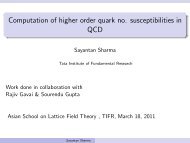
Let us consider the equilibrium density profile ρ(r) and a reference density profile ρ0(r) for the same 

system. Assume the linear parametrization 

ρλ(r) =ρ0(r)+λ[ρ(r) − ρ0(r)] = ρ0(r)+λ∆ρ(r) λ ∈ [0 : 1] 

From the definition of c (1) and c (2) as functional derivative we can write 

� 1 � 

Fex[ρ] =Fex[ρ0] − kBT dλ d 3 r ∆ρ(r)c (1) (r;[ρλ]) 

c (1) (r;[ρ]) = c (1) (r;[ρ0]) + 

Using the second in the first and noticing that 

we get 

Fex[ρ] = Fex[ρ0] − kBT 

0 

� 1 

0 

� 

dλ 

For homogeneous systems with ideal gas reference state 

χ (0) 

T 

χT 

lunedì 7 dicembre 2009 

= 

� ∂βP 

∂ρ 

� 

− kBT 

T 

� 1 

0 

� � 

∂βµ 

= ρ 

∂ρ 

� 

� 

dλ(1 − λ) 

T 

� 

=1− ρ 

0 

d 3 r ′ ∆ρ(r ′ )c (2) (r, r ′ ;[ρλ]) 

� 1 � x � 1 

dx dy g(y) = dx (1 − x) g(x) ∀g(x) 

d 3 r ∆ρ(r)c (1) (r;[ρ0]) 

0 

d 3 rd 3 r ′ ∆ρ(r)c (2) (r, r ′ ;[ρλ]) ∆ρ(r ′ ) 

c (1) (ρ) =−βµex = 

0 

� ρ 

d 3 rc (2) (r, ρ) =1− ρ ĉ (2) (k = 0) 

0 

dρ ′ 

� 

d 3 rc (2) (r, ρ ′ )

The effective one-component system 

Integral equations approach and inversion procedure: 

remember that 

Fex[ρ] = Fex[ρ0] − kBT 

− kBT 

and consider the uniform reference system ρ0(r)=ρ0: c (1) (r,ρ0)=-βµex 

Add the ideal contribution and switch back to ΩV 

ΩV [ρ] =Ω0(ρ0) + 

� 

� 1 

0 

− kBT 

� 

� 

dλ(1 − λ) 

d 3 rρ(r)Φ(r)+kBT 

� 1 

0 

� 

dλ(1 − λ) 

d 3 r ∆ρ(r)c (1) (r;[ρ0]) 

d 3 rd 3 r ′ ∆ρ(r)c (2) (r, r ′ ;[ρλ]) ∆ρ(r ′ ) 

� 

d 3 r 

� 

ρ(r)log ρ(r) 

ρ0 

� 

− ∆ρ(r) 

d 3 rd 3 r ′ ∆ρ(r)c (2) ([ρλ], r, r ′ )∆ρ(r ′ ) 

Replacing c (2) ([ρλ],r,r’) by c (2) (r-r’) of the uniform system, the equilibrium condition for the functional 

provides the HNC equation 


ρ(r) =ρ0exp 

� 

−βΦ(r)+ 

� 

d 3 r ′ c (2) (r − r ′ )∆ρ(r ′ � 

) 

HNC


Percus (1962): consider one particle in the system as a test particle 

φ(r) =v(r) the inter-particle potential 

ρ(r) =ρ0g(r); ∆ρ(r) =ρ0h(r) of the uniform system 

HNC+OZ: g(r) =exp {−βv(r)+h(r) − c(r)} HNC closure for homogeneous systems 

Percus-Yevik (PY): g(r) =e −βv(r) [g(r) − c(r)] PY, very accurate for hard spheres 

Ideal gas limit: 

lim g(r) =e 

ρ→0 −βv(r) 

HNC and PY provide a link between the pair structure g(r) and the two-body potential v(r) in a 

uniform system, if supplemented by: 

Theorem (Henderson, Phy. Letts. 49A, 197 (1974)): in a quantum or classical fluid with only pairwise 

interactions, and at fixed thermodynamic conditions, the pair potential v(r) that give rise to a given 

radial distribution function g(r) is unique, up to a constant. 

In other words, if a potential exists which generate a given g(r), this potential is unique up to a 

constant. 

g(r) ⇐==⇒ v(r) 

lunedì 7 dicembre 2009


Inverse problem: from a measured g(r) to a two body effective interaction v(r) 

Theoretical basis for Boltzmann inversion, HNC inversion and Modified-HNC inversion 

HNC inversion: 

In a one component system, the original pair potential is recovered if the inversion procedure is 

exact (or fully converged for the iterative solutions). (Reatto et al. Phys. Rev. A33, 3541 (1986)) 

In a multi component system, inversion of radial distribution functions gαβ(r) provides effective twobody 

potentials vαβ(r) between species α and β. 

- effective potentials are state dependent. 

- effective potentials are obtained at finite density, at variance with ω2(r) of the diagrammatic 

expansion which considered only two particles (zero density limit). 

In a two component system, the effective pair potential v11(r) obtained from the inversion procedure 

is a resummation of all n-body terms in the diagrammatic expansion of the free energy. 

The two body term of the diagrammatic expansion is only the zero density limit of the effective pair 

potential 

βv(r) =− log[g(r)] + h(r) − c(r) − log[g(r)] 

φ11(Rij)+ω2(Rij; z2) = lim 

ρ1→0 veff 

11 (Rij; ρ1,z2) 

Drawbacks: 

• the knowledge of the relevant g(r) is needed. Only possible for not too extreme size ratios. 

• computing thermodynamics with density dependent potentials is more cumbersome 


Single chain conformations 

Polymeric systems 

Polymers are macromolecules build up by repeating chemical units (monomers) bonded together in 

various topologies. 

Relevant length scales for very long chains: 

• the atomic length scale relevant for the local chemistry of monomers 

• the Kuhn or persistence length is an intermediate length scale at which the atomistic details are lost 

and a number of chemical monomers have been coarse-grained into a single physical monomer. 

• the chain size is the macroscopic length over which the polymer spread in space : end-to-end 

distance or radius of gyration 

Primitive polymer model: 

Physical monomers resolution: a sequence of point particles connected in a fixed topology. 

Interactions: 

• bond interactions between adjacent monomers along the chain C.N. Likos / Physics Reports 348 (2001) 267}439 

• steric interaction between any pair of monomers 

particle positions ri i ∈ [0,N] 

chain center of mass RCM = 1 

N +1 

N� 

i=0 

position relative to CM si = ri − RCM i ∈ [0,N] 

bond vectors ℓi = ri+1 − ri 

end-to-end vector R = rN − r0 = 


gyration radius R 2 g = 1 

N +1 

N� 

i=0 

N� 

i=1 

ri 

ℓi 

s 2 i = 

1 

2(N + 1) 2 

� 

|rij| 2 

i,j 

Fig. 8. A simple picture for the description of the conformations of a polymer chain. The "lled cir

This implies that the quantity = (R), where = (R)dR denotes th 

� � 

with end-to-end distances lying between R and R#dR, has the fo 

Single chain 

For very large N (N⟶∞), chains are self-similar objects, meaning that the property of part of the chain 

are identical to the property of the entire chain under a proper rescaling of lengths. 

The physics of chains is expressed in terms of scaling laws 

R =< R 2 > 1/2 ∼ N ν 

D ∼ N −ν′ 

end-to-end distance 

CM diffusion coefficient 

Fig. 9. An instantaneous conformation of a self-avoiding chain. The two monomers located at 

B experience a steric repulsion, denoted by the dotted line, and hence develop a correlation in their po 

Ideal chain model: their separation along the chain is many times larger than the persistence length l . 

� 

• bonds of fixed length a or with gaussian distribution of 

length around a This implies that the quantity = (R), where = (R)dR denotes the total number o 

• steric interaction is absent 

� � 

with end-to-end distances lying between R and R#dR, has the form [118] 

By central limit theorem: = (R)JR�exp� ! 

� 3R� 

2Na�� . 

The prefactor R� on the right-hand side of Eq. (3.6) above arises from geometry; the 

be identi"ed with a Boltzmann factor, thus giving rise to an elastic free energy F (R 

� 

chain, which is entropic in nature and reads as [29] 

F (R)"F(0)# 

�� 3k � ¹ R� 

2 Na� , 

Fig. 9. An instantaneous conformation of a self-avoiding chain. The two monomers located at po 

B experience a steric repulsion, denoted by the dotted line, and hence develop a correlation in their posit 

their separation along the chain is many times larger than the persistence length l . 

� 

This implies that the quantity = (R), where = (R)dR denotes the total number of 

� � 

with end-to-end distances lying between R and R#dR, has the form [118] 

= (R)JR�exp� ! 

� 

where F(0) is an unimportant constant. The last equation allows for the interpretatio 

chain as an elastic spring with spring constant k"3k ¹/Na�. 

� 3R� 

2Na�� . 

The prefactor R� on the right-hand side of Eq. (3.6) above arises from geometry; the ex 

be identi"ed with a Boltzmann factor, thus giving rise to an elastic free energy F (R) 

� 


F (R)"F(0)# 

�� 3k � ¹ R� 

2 Na� , 

= (R)JR�exp� ! 

� 

Elastic free energy of an ideal chain 

where F(0) is an unimportant constant. The last equation allows for the interpretation 


Self avoiding walk model (SAW): 

� 

The physical reason for the fact that the measured exponent � in real polymers devia 

• bonds of fixed length a or Gaussian with gaussian value � distribution "1/2 is thatof the RW-model (and all its re"nements) fail to capture 

length around a 

� 

the chain cannot intersect itself, it is self-avoiding. The microscopic origin of the self-av 

• steric monomer-monomer in the interaction: steric repulsions between the monomers which prohibit them from approachin 

3R� 

2Na�� . 

The prefactor R� on the right-hand side of Eq. (3.6) above arises fro 

be identi"ed with a Boltzmann factor, thus giving rise to an elastic 


F (R)"F(0)# 

�� 3k � ¹ R� 

2 Na� , 

where F(0) is an unimportant R = constant. a The last equation allows for 


� 

The physical reason for the fact that the measured exponent � in r 

Gaussian value � "1/2 is that the RW-model (and all its re"neme 

� 

the chain cannot intersect itself, it is self-avoiding. The microscopic o 

in the steric repulsions between the monomers which prohibit them 

close to one another. Though the steric forces are short-range in n 

e!ect along the chain, irrespective of the persistence length l .� No m 

� 

other two monomers lie in the polymer sequence, once they ap 

interactions enforce a correlation in their positions, as shown in 

interaction between monomers, v (r ,r ) is usually approximated 

�� 

[120}122]: 

v (r , r )"v k ¹�(r !r ) , 

�� √ N −→ νid =0.5 


close 

The physical 

to one another. 

reason 

Though 

for the fact 

the 

that 

steric 

the 

forces 

measured 

are short-range 

exponent � 

in 

in 

nature, 

real polymers 

they have 

dev 

a 

Gaussian 

e!ect along 

value 

the 

� 

chain, 

"1/2 is that the RW-model (and all its re"nements) fail to captur 

� irrespective of the persistence length l .� No matter how far awa 

the chain cannot intersect itself, it is self-avoiding. The microscopic � 

other two monomers lie in the polymer sequence, once they approach origin of each the self- othe 

ininteractions the steric repulsions enforce a between correlation theinmonomers their positions, which as prohibit shownthem in Fig. from9. approachi The exclu 

close interaction to one between monomers another. monomers, Though are lost [119]. the v steric (r ,r forces ) is usually are short-range approximated in nature, by a delta-functio they have 

�� 

� The persistence length l � is de"ned as the length along the chain in which o

Single chain 

Flory’s mean field argument for SAW: 

the number of monomer that can fit into a volume R 3 without overlap is R 3 /v0. The probability that 

one segment will not overlap with another is (1-v0/R 3 ). For N(N+1)/2 distinct pairs we have 

Pint(R) ∝ 

� 

1 − v0 

R3 �N(N+1)/2 � 

N(N + 1) 

= exp 

2 

Free energy: βFtot = βFel + βFint = 3R2 

2Na2 + N 2v0 2R3 log(1 − v0/R 3 � 

) 

� exp 

� 

− N 2v0 2R3 � 

equilibrium state (minimum): R 5 = v0a 2 N 3 → R ∼ N 3/5 =⇒ νsaw = 3 

5 =0.6 

At d dimensions: νsaw = 3 

d +2 → νsaw = 1 

2 

for d =4 

At d=4, the excluded volume is negligeble. 

Renormalization Group study at d=4 and (4-ε) expansion provides: 

in agreement with MC simulations and close to Flory’s value. 


νsaw =0.588

Lattice model of a chain in solvent 

nearest-neighbors attractions: 

monomomer-monomer 

monomer-solvent 

solvent-solvent 

Single chain: effect of the solvent 

−ɛppNpp 

−ɛpsNps 

−ɛssNss 

Average energy from these interactions: 

E = −ɛppNpp − ɛpsNps − ɛssNss 

• Npp=average number of pp contacts 

• Nps=average number of ps contacts 

• Nss=average number of ss contacts 

monomer 

solvent particle 

Monomers uniformely distributed inside R 3 : φp=v0N/R 3 

Fig. 10. A lattice model of a chain in a solvent. The monomers are denoted by the black circles and the 

by the white ones. For the sake of simplicity, these two species are taken to have the same size. 

with z being the coordination number of the lattice and �� being given by 

��"(� �� #� �� )/2!� �� . 

βE(R) =− N 2v0 βz 

χ; χ = 

R3 2 (ɛpp + ɛss − 2ɛps) 

Free energy: βFtot = βFel + βFint = 3R2 


The ideas employed in the derivation of Eq. (3.16) above are the same with thos 

Section 2 in deriving an e!ective Hamiltonian: the degrees of freedom of one type o 

solvent molecules) are traced out and an e!ective Hamiltonian for the remain 

monomers) is obtained, with coupling constants depending on some external param 

parison between Eqs. (3.11) and (3.16) shows that the e!ect of the solvent is to 

a renormalized, temperature-dependent excluded-volume parameter, v(¹), which rep 

parameter 2Nav : 

� 2 + N 2v 2R3 ; v = v0(1 − 2χ) 

v � Pv(¹)"v � (1!2�) . 

C.N. Likos / Physics Reports 348 (2001) 267}439 

Npp = 1 

2 zNφp 

Nps = zN(1 − φp) 

Nss = Ns(Ns − 1) 

2 

− Npp − Nps 

The origin of the nearest-neighbor attractions modeled by the parameters � ��

Single chain: effect of the solvent 

three distinct regimes 

a) good solvent conditions: (1-2χ)>0 high T v>0 and ν=⅗ 

b) poor solvent conditions: (1-2χ)

Polymer solutions 

System of M chains of the same length N in a solvent in a volume V. 

The relevant thermodynamics variable is the chain density ρ=M/V, 

ρ*=3/(4πR3 )= chain overlapping density ~N-3ν In good solvent we can distinguish three regimes 

a) Dilute solutions: ρ/ρ*1 large monomer fluctuations 

c) Concentrated regime: N ρ ~ 1 small monomer fluctuations 

C.N. Likos / Physics Reports 348 (2001) 267}439 307 

Fig. 11. The three concentration regimes for polymer solutions: (a) dilute, where the average separation d between 

the coils is much larger than the typical size R H of the coil; (b) semidilute, above the overlap concentration c H ; 

(c) concentrated solution, above the concentration c HH . 

c*=monomer concentration at overlap: c*=N ρ* ~N 

where r denotes the position vector of the nth monomer in the chain and the index n is treated as 

� 

a continuous variable. The "rst term in this Hamiltonian is the elastic contribution associated with 

the ideal chain alone and the second term encapsulates the excluded-volume interactions. In this 

1-3ν


Flory-Huggins: mean field theory of the solution provide qualitively correct phase behaviour which 

become quantitative at high concentrations (negligible fluctuations) 



Scaling theory: chains are self-similar, the physics is unchanged if one groups λ monomers together and 

rescale the distances 

N → λ −1 N and a → λ ν a 

Osmotic pressure: f is dimensionless 

Π= ckBTf(a 3 c, N) 

c → λ −1 c =⇒ f(a 3 c, N) =λ −1 f(λ 3ν−1 a 3 c, λ −1 N)= 1 

N ˆ f(a 3 cN 3ν−1 ) 

In terms of the overlap monomer concentration Π(c) = ckBT 

N ˆ c f 

∗ = a −3 N 1−3ν 

- in the dilute regime van’t Hoff’s law implies 

- in the semidilute regime Π must become independent on N: 

Π(c) ∼ ckBT 

N 

� 

c 

c∗ �1/(3ν−1) ∼ c 9/4 

lim 

x→0 

ˆf(x) = 1 

good solvent 

ˆf(x) ∼ x α 

α = 

� 

c 

c∗ � 

1 

(3ν − 1) 

Confirmed by experiments and at variance with the c 2 behaviour predicted by mean field theory. 



Chain size in good solvent: 

dilute regime: ν=⅗ excluded volume statistics at all lengths scale 

concentrated regime: ν=⅗ at intermediate length scales below the screening length ξ 

ν=½ at larger length scale 

R~ξ 1-1/2ν N 1/2 ideal chain statistics 

semidilute regime from scaling: R(c) =R(0) ˜ f 


c > c ∗ 

c ∗ = a −3 N 1−3ν 

R(c) ∼ aN ν � c 

c ∗ 

R(c) ∼ aN ν � c 

c∗ � 1−2ν 

6ν−2 

3 − 

ξ ∼ c 4 

→ δ = 

1 − 

∼ c 8 

� δ 

� 

c 

c∗ � 

∼ N 1/2 

1 − 2ν 

6ν − 2 

= −1 

8 

= aN ν ˜ f 

� 

c 

c∗ � 

(ν =3/5) 

in agreement with experiments

quila, I-67010 L’Aquila, Italy 

y of L’Aquila, I-67010 L’Aquila, Italy 

ierre Hansen 

VOLUME 85, NUMBER 12 P H Y S I C A L R E V I E W L E T T E R S 18 SEPTEMBER 2000 

ensfield Road, Cambridge CB2 1EW, CanUnited Polymer Kingdom Coils Be Modeled as “Soft Colloids”? 

ed 8 October 2007; published online 1 November 2007� 

ent Zero description density limit: of polymer interaction solutions potential is presented, between two isolated chains. 

(Received based 26 May on2000) soft, 

sIn between this limit bonded the potential and nonbonded is effective segments. The number 

at the segment density does not exceed 

βvpp(R1 − R2) 

their 

=− 

overlap 

log 

threshold, 

[gpp(R1 − R2)] 

s to be explored deep into the semidilute regime. This quantitative 

shown 

gpp(R) is 

to 

the 

preserve 

pair distribution 

known scaling 

function 

laws of 

of 

polymer 

the two 

solutions and 

mplitudes, while leading to a orders-of-magnitude increase in the 

centres of mass at distance R. 

owing analytic calculations PACS numbers: 61.25.Hq, of structural 61.20.Gy, 82.70.Dd and thermodynamic 

stitute of Physics. A statistical �DOI: description 10.1063/1.2803421� 

of polymer solutions in complex 

RGT provides a universal Gaussian Core Potential: 

318 C.N. Likos / Physics Reports 348 (2001) 267}439 

v�r� 

kBT Fig. 14. A snapshot from a simulation involving two self-avoiding polymers. In this con"guration 

the two chains (denoted by the big sphere) coincide, without violation of the excluded-volume co 

Arben Jusu".) 

where � is an energy scale of the order of k ¹ and � is a length scale proportion 

� 

gyration R of the chain. The e!ective potential is entropic, i.e., the energ 

� 

proportional to the temperature and the latter is a thermodynamically irre 

for the polymer solution, as expected for an athermal solvent: all monome 

� A exp�− ��r/Rg�2�, �1� 

where A�1.75 and ��0.80. For finite L, the MC data 6 for 

the amplitude A can be fitted, for L�100 by A�L�=A � 

+a/L � , with A�=1.75, a=1.5, and �=0.33, while the coefficient 

� turns to be independent of L. The softness of the 

repulsive interaction, characterized by a modest free energy 

penalty of �2kBT at full overlap �r=0� of two polymers, 

reflects the low average monomer concentration c�L 1−3� 

�L−0.77 A(N) = A∞ + 

inside each coil for long chains. 

* 

a 

N σ 

ingly, well into the semidilute regime. A related “soft par- 

geometries, such as the colloid-polymer mixtures which ticle” picture has been applied to polymer melts and blends 

have recently received much experimental attention [1–3], [9], but the corresponding phenomenological implementa- 

generally relies on a nanometer scale segment representation differs substantially from the present first principles 

tion of the polymer coils, a computationally very demand- approach. 

ing task except in the special case of ideal (nonintersecting) We consider a popular model for polymers in a good 

polymers obeying Gaussian statistics [4]. This obviously solvent [10], namely, N excluded volume polymer chains 

follows from the fact that, although the colloidal particles of L segments undergoing nonintersecting self-avoiding 

may reasonably be modeled by hard impenetrable spheres walks (SAW) on a simple cubic lattice of M sites, with 

or other complex shapes lacking internal structure, each periodic boundary conditions. The packing fraction is 

polymer coil involves L segments which must satisfy a equal to the fraction of lattice sites occupied by poly- 

nonintersection constraint. It thus appears natural to atmer segments, c � N 3 L�M, while the concentration of 

tempt a mesoscale coarse graining, whereby polymer coils polymer chains is r � c�L � N�M. For a single SAW 

A∞ =1.75; a =1.5; σ =0.33 

interact via effective pair potentials acting between their chain, the radius of gyration Rg � L 

centers of mass (CM). Since polymers can interpenetrate, 

α = 0.80 

the effective potential by�r� is expected to be soft, with a 

rangeRg of the order = of chain the radius of gyration of gyration Rg of individual 

coils. Such a coarse-grained description has been a longtime 

goal in the statistical mechanics of polymer solutions, 

dating back to the first attempts by Flory and Krigbaum [5] 

n , where n � 0.6 is 

the Flory exponent [10]. The overlap concentration r� , 

signaling the onset of the semidilute regime, is such that 

4pr�R3 g�3 � 1, and hence r� � L23n . We have carried 

out Monte Carlo (MC) simulations for chains of length 

L � 100 and L � 500, and covered a range of concentrations 

up to r�r� � 5. The pair distribution function g�r� 

nd thermodynamic 

ns, both in the bulk 

ively understood in 

de Gennes–Pincus 

whenever From MC the calculations char- for N>100: 

ution �e.g., the corent 

is significantly 

an isolated polymer 

atic coarse-graining 

n is divided into a 

ontaining the same 


A. A. Louis, 1 P. G. Bolhuis, 1 J. P. Hansen, 1 and E. J. Meijer 2 

1Department of Chemistry, Lensfield Road, Cambridge CB2 1EW, United Kingdom 

2Department of Chemical Engineering, University of Amsterdam, 

Nieuwe Achtergracht 166, NL-1018 WV Amsterdam, The Netherlands 

We map dilute or semidilute solutions of nonintersecting polymer chains onto a fluid of “soft” particles 

interacting via a concentration dependent effective pair potential, by inverting the pair distribution 

function of the centers of mass of the initial polymer chains. A similar inversion is used to derive an 

effective wall-polymer potential; these potentials are combined to successfully reproduce the calculated 

exact depletion interaction induced by nonintersecting polymers between two walls. The mapping opens 

up the possibility of large-scale simulations of polymer solutions in complex geometries.

ecome slightly longer ranged at higher densities implies 

that the pressure scales with an exponent slightly higher 

than 2, so that the equation of state (e.o.s.) is consistent 

with the well-known r2.25 law [10], and reproduces the 

FIG. 7. The effective polymer CM pair potential v(r;� b) derived from a 

HNC inversion of g(r) for different densities. The x-axis denotes r/R g , 

where R 3 

g is the radius of gyration of an isolated SAW polymer. �Inset� The 

value of the effective polymer CM pair 1 potential at r�0, as a function of 

Coarse-grained model for polymer solutions 

Finite density: HNC inversion is very accurate because of the softness of the potential 

βv(r; ρ) =− log[g(r)] + h(r) − c(r) 

Remarks: 

• the pair correlation decreases with increasing 

density (like for quantum particles) confirming that 

in the melt regime, polymers are uncorrelated. 

• the effective interaction at zero distance is 

always ~2kT and has a non monotonous behaviour 

with ρ 

• the effective potential is only moderately density 

dependent and is well fitted by a sum of gaussians 

• the effective range of the interaction tends to 

increase with ρ, and the potential develops a small 

amplitude negative tail for r>>Rg 


density � b /�*. The maximum of the potential initially increases before 

decreasing at high concentration. 

2 

r 

0 

0 1 2 3 

r/Rg 1 

ρ/ρ∗ = 0 

ρ/ρ∗ = 0.54 

ρ/ρ∗ = 1.09 

ρ/ρ∗ = 2.18 

ρ/ρ∗ = 4.35 

0 

0 1 2 3 4 5 

2 v(r;� b). For example, leaving them out can easily induce 

a 5% change in the pressure. It is, therefore, paramount to 

include these effects in �quasi�-analytical representations of 

the effective potentials. For that reason, a simple fit to a 

Gaussian or a sum of Gaussians is not accurate enough to 

reproduce the potentials and hence the thermodynamics of 

the SAW polymer systems and consequently, we chose to 

use an interpolation spline fit to describe the potentials. First, 

the raw effective potential data were fitted to a Gaussian, 

. �10� 

βv(r/R g ) 

v est�r��a 0e �a 1 r2 

g(r/R g ) 

0.5 

r/R g 

Subsequently, FIG. 1. The theeffective difference polymer �v(r;� CM pair b)�v(r;� potential b)�v by�r�Rg� est(r) 

was fitted derived byfrom employing an HNCainversion least squares of g�r�Rg� splinefor procedure different densi- with 

ties. The x axis denotes r�Rg, where Rg 8 nodes �the ‘‘dfc’’ routine of the slatecislibrary the radius of gyration 

of an isolated SAW polymer. Inset: The polymer CM pair distribution 

function g�r� calculated for L � 500 SAW polymers 

and used to generate by�r�. 

52 �. The val- 

effective wall 

wall-polymer 

sulting in 

FIG. 9. The eff 

creases as a func 

tive radius of gyr 

βφ(z/R g ) 

bf�z� � b 

6 

4 

2 

0 

0 

FIG. 2. The w 

HNC inversion 

h�z� � r�z��r 

adsorptions G 

R22 ues of the no 

boundaries r� 

spline fit wer 

�0. We optim 

x-axis using a 

the fits are av 

Note that 

v(r;� b) is plo 

tion of isolate 

dense solution 

mers contract 

as shown in F 

The accu 

performing a 

the ‘‘soft coll 

pair distributi 

compared wit 

g , respective

tail for r significantly larger than Rg [4, 11]. The link with thermodynamics is via the 

Link with thermodynamics via the compressibility relation 

sibility relation [9], which allows the osmotic pressure P to be expressed as 

� ρ 

β P(ρ) = [1 − ρ 

0 

′ ĉ(k = 0; ρ ′ )]dρ ′ 

(6) 

k) is the Fourier transform of c(r). Use of the effective pair potential in conjunction 

virial and energy equations is meaningless [12]. The equations of state calculated 

simulations of the full monomer level polymer representation and from simulations 

the much less CPU-intensive effective potential representation agree within numerical 

ties, underlining the adequacy of the HNC inversion procedure for such ‘soft’ 

particles. Well into the semi-dilute regime (ρ ≫ ρ∗ ) the slopes of the calculated 

of state agree with the des Cloizeaux scaling prediction β P ≈ ρ3ν/(3ν−1) ≈ ρ9/4 , 

= 0.588 ≈ 3/5 istheFlory exponent for the radius of gyration in good solvent 

Lν )[10]. 

lecting the density dependence of v2(r), i.e. extending the low-density Gaussian 

all densities, brings us back to the ‘Gaussian core model’ (GCM) first introduced 

ger [13], which exhibits interesting behaviour at low temperatures (β∗ ≫ 1) [14]. 

gime relevant for polymer solutions (β∗ ≈ 1) the model leads to ‘mean field fluid’ 

r at sufficiently high density,where the random phase approximation,c(r) = −βv2(r) 

a quadratic equation of state for ρ ≫ ρ∗ [14, 15]: 

β P = ρ + 1 

2β ˆv2(k = 0)ρ 2 . (7) 

ating the ρ-dependence of v2 is found from simulation to change the asymptotic 

viour into des Cloizeaux scaling ρ9/4 Remarks: 

• it is well known (Stillinger) that the 

‘gaussian core model’ has an EOS quadratic 

in density which violates scaling 

• incorporating the density dependence into 

the potential restore the correct des 

Cloizeaux scaling ρ 

. Asaby-product of the GCM, we have 

d a multiple occupancy lattice model, which also gives rise to interesting microphase 

n [16]. 

good to poor solvent conditions 

9/4 

on the much less CPU-intensive effective potential representation agree within numerical 

tainties, underlining the adequacy of the HNC inversion procedure for such ‘soft’ 

ive particles. Well into the semi-dilute regime (ρ ≫ ρ 

• the inversion procedure does not provide 

the volume term necessary to compute the 

free energy of the effective model. However 

the observed agreement between OES for 

the full monomer and the effective 

polymers suggests that this term is negligibly 

small 

∗ ) the slopes of the calculated 

ion of state agree with the des Cloizeaux scaling prediction β P ≈ ρ3ν/(3ν−1) ≈ ρ9/4 , 

e ν = 0.588 ≈ 3/5 istheFlory exponent for the radius of gyration in good solvent 

bLν )[10]. 

eglecting the density dependence of v2(r), i.e. extending the low-density Gaussian 

to all densities, brings us back to the ‘Gaussian core model’ (GCM) first introduced 

illinger [13], which exhibits interesting behaviour at low temperatures (β∗ ≫ 1) [14]. 

regime relevant for polymer solutions (β∗ ≈ 1) the model leads to ‘mean field fluid’ 

iour at sufficiently high density,where the random phase approximation,c(r) = −βv2(r) 

to a quadratic equation of state for ρ ≫ ρ∗ [14, 15]: 

β P = ρ + 1 

2β ˆv2(k = 0)ρ 2 . (7) 

porating the ρ-dependence of v2 is found from simulation to change the asymptotic 

haviour into des Cloizeaux scaling ρ9/4 . Asaby-product of the GCM, we have 

oped a multiple occupancy lattice model, which also gives rise to interesting microphase 

ation [16]. 

om good to poor solvent conditions 

ow turn our attention to the case where adjacent monomers attract, i.e. ɛ �= 0 or β∗ > 0. 

attraction is solvent induced, and the quality of the solvent deteriorates as β∗ increases, 

g to contraction of the polymer coils. At the θ temperature (β∗ θ = ɛ/kBTθ), repulsion and 

tion between polymers cancel, at least in the low-density limit, so the polymers exhibit 

aling behaviour of ideal polymers (Rg ∼ L1/2 ). Below Tθ , polymer coils collapse 

lobules (Rg ∼ L1/3 semidilute regime. The difference between the two disbution 

functions shows an oscillation at small r. Because 

s occurs in the same way for both densities it is possibly 

roduced by the inversion procedure. Even so, the differce 

between the two distribution functions is still typically 

s than �0.01. We conclude that the HNC inversion produre 

yields very accurate effective potentials for soft parles, 

capable of describing the structure of the fluid with an 

solute error of less than �0.01. 

In a previous paper 

), and phase separation occurs into polymer-rich and polymer-poor 

40 we have shown that the HNC clore 

is very accurate when applied to the Gaussian model, 55 

ereby particles interact via the repulsive potential v(r) 

� exp��(r/Rg) 2 �, and is in fact quasiexact in the regime 

evant to the effective potentials shown in Fig. 7. 56 Even 

much cruder RPA closure, c(r)��v(r), yields semiantitatively 

accurate results for correlations and thermodymics 

in the regime of interest. Thus polymer solutions in 

dilute or semidilute regime fall into the class of mean 

ld fluids according to the nomenclature introduced in Ref. 

. 

The inversion procedure guarantees that the two-body 

rrelations are accurately reproduced by the effective potenl, 

but this does not necessarily imply that higher order 

rrelations are also well represented. As a first test we permed 

preliminary simulations of the three-body correlation 

� ln Z�N,L,D,H� 

�2 �D 

ctions for both full SAW walks and our soft particles. The 

�H 

o approaches lead to identical results within statistical ers, 

implying that higher order correlations are much more 

curately reproduced than one might initially expect. We 

ve also performed some preliminary calculations of the 

02 J. Chem. Phys., Vol. 114, No. 9, 1 March 2001 Bolhuis et al. 

ee-body lunedì 7 dicembre interaction 2009 

v3(r 1,r2,r3). Even at full overlap of 

FIG. 11. Log–log plot of the e.o.s. Z��/� b as a function of the density for 

L�500 polymers. The soft-particle e.o.s. gives a good representation of the 

full SAW polymer simulations. At the highest densities there is a slight 

deviation from the expected des Cloizeaux (� b /�*) 1/(3��1) scaling law 

which we attribute to the effects of a finite monomer concentration c. Also 

shown is the RG e.o.s. of Ohta and Oono �Refs. 60, 61�. 

�D �2 �ln Z�N,L,D,H��ln Z�N,L,D,H�1��. �11� 

The model is modified by associating an additional repulsive 

potential �ln � with each occupied site in the plane x�H, 

where 0��1. The partition function then becomes


Same strategy to compute hard wall-polymer effective interactions 

4304 J. Chem. Phys., Vol. 114, No. 9, 1 March 2001 J. Chem. Phys., Vol. 114, No. 9, 1 March 2001 Bolhuis et al. 

FIG. 13. The wall–polymer CM density profile h(z)��(z)/� b�1 for SAW 

polymers at different bulk concentrations. From h(z) we can calculate the 

corresponding polymer absorptions � and find ��0, 0.094, 0.13, 0.16, 

and 0.20 in units of R g �2 , respectively. The relative absorptions are 

��/� b�0.84, 0.59, 0.41, 0.27, and 0.14 R g , respectively, and decrease 

with increasing density as expected. 

�� ex /A� 

�� 

�� b� 0 

� 

h�z�dz, �17� 

where �ex /A is the excess grand potential per unit area and 

� the chemical potential of the polymers. As the density 

increases, more polymer is adsorbed at the wall as expected, 

but the relative adsorption, �/� b , decreases. 


length 2 in the semidilute regime. Although the profiles do not 

show such a clear correlation-induced oscillation as the CM 

profiles, there is nevertheless still a small maximum in the 

depletion layer as illustrated in the inset of Fig. 14. The peak 

in the monomer profile is less than 1% of the bulk density, 

and seems to decrease with higher overall polymer concentration. 

The range is about R g , implying that it arises from 

correlations between polymer coils. We observe only one 

peak, although due to statistical noise, we cannot rule out the 

possibility of more oscillations in the density profiles. Recently 

self-consistent field calculations, valid for polymers in 

a theta solvent, found a similar small oscillation in the monomer 

profiles. 64 

B. Deriving �„z;� b… from �„z… 

From a knowledge of the concentration profile �(z), and 

the bulk direct correlation function between polymer CM’s, 

cb(r), one may extract an effective wall–polymer potential 

�(z;� b) by combining the wall–polymer OZ relations 48 with 

the HNC closure. For a binary mixture of two components 

labeled 0 and 1, in which component 0 is infinitely dilute 

(x 0→0), the Ornstein–Zernike equations become 48 

Sec. IV A�, together with 

b� 

Eq. �20�, we are able to extract 

�(z;� h11�1,2��c 11�1,2�� h11�1,3�c 11�2,3�d3, �18a� 

b) from the density profiles. In order to calculate the 

integral in Eq. �20�, we use the procedure outlined by Sullivan 

and b� h10�1,2��c Stell. 10�1,2�� h11�1,3�c 10�2,3�d3, �18b� 

b� h01�1,2��c 01�1,2�� h01�1,3�c 11�2,3�d3, �18c� 

66 FIG. 15. The wall–polymer potential �(z;� b) as obtained from the inversion 

of h(z) via the HNC expression, Eq. �20�. 

In contrast to the inversion of the bulk g(r), 

where we had to iterate until convergence, the wall–polymer 

inversion requires only one step since cb(r) is given once 

and for all. Results for various bulk concentrations are plot- 

F 

l 

� 

S 

i 

t 

d 

n 

t 

t 

o

teraction range. 


oid representation of the interacting polymer coils, and the 

ccuracy of the HNC inversion for polymer coils near a hard 

all. 

I. DEPLETION POTENTIAL BETWEEN TWO WALLS 

. Full SAW simulations 

One of the aims of this work is to show that the soft 

article description of the polymers provides a useful route 

o the colloid–colloid depletion potential in mixtures of coloidal 

particles and nonadsorbing polymers. Calculating 

hese depletion interactions poses a severe test of the soft 

olloid representation. 

As a first step we calculate the depletion potential beween 

two planar walls, which can ultimately be applied to 

pherical colloids through the Derjaguin approximation. We 

onfined the polymers within a slit of width d, and, using 

irect grand-canonical simulations of the full SAW polymer 

odel, we computed the osmotic pressure exerted by the 

olymer coils on the walls. The insertion of polymers was 

chieved by the configurational bias Monte Carlo 

echnique. 33 thermodynamic integration technique similar to the one explained 

in Sec. IV B. Details of these simulations can be 

found in Ref. 67. The interaction free energy per unit area A, 

�F/A, is then obtained by integrating the osmotic pressure 

306 as aJ. function Chem. Phys., of d, Vol. 114, No. 9, 1 March 2001 Bolhuis et al. 

� 

�F�d�/A�� dz��z��, �21� 

d 

where �(�) denotes the bulk osmotic pressure �b . These 

explicit SAW simulations are rather computer intensive, and 

were only carried out for L�100. 

2 

FIG. 18. Depletion free-energy �F(d)/Rg between two plates separated by 

d, for three densities, �b /�*�0.95, �b /�*�0.58, �b /�*�0.24. The symbols 

denote the ‘‘exact’’ MC simulations, while the dashed, dashed–dotted, 

and solid lines are the soft-colloid simulations for the same densities. �Inset� 

�F(d)/�F(0) for the SAW simulations, the solid lines are to guide the eye. 

The long-dashed line is the ideal Gaussian polymer result calculated in the 

The �osmotic� pressure �(d) was calculated for Appendix. Note that the range decreases with density, and that, even for the 

lowest density, the AO ideal polymer approximation overestimates the in- 

ifferent values of the spacing d between the walls by a teraction range. 

hermodynamic integration technique similar to the one exlained 

in Sec. IV B. Details of these simulations can be 

ound in Ref. 67. The interaction free energy per unit area A, �2Rg where the soft particle picture shows a larger repulsive 

F/A, is then obtained by integrating the osmotic pressure barrier. The barrier height is, however, small compared to the 

67 

�2Rg where the soft particle picture shows a larger r 

barrier. The barrier height is, however, small compare 

attractive minimum at contact, which agrees well w 

‘‘exact’’ data, as does the slope of the attraction. 

Liquid state theories for fluids with repulsive p 

particle interactions predict a repulsive barrier, 

B. Effective potential simulations 

In the soft colloid picture, the interactions of the polymer 

CM’s with each other, v(r;� b), and with a wall, �(z;� b), 

are calculated once with the HNC inversion procedures from 

the g(r) and �(z) of a full SAW polymer simulation at the 

bulk density �b . These potentials are then used in grandcanonical 

MC simulations of soft particles between two 

walls. The imposed chemical potential is chosen such that 

for infinitely separated walls the bulk density is recovered. 

The �osmotic� virial pressure is measured as a function of 

wall separation d, and the interaction free energy per unit 

area �F/A, is again obtained by integration of the pressure 

via Eq. �21�. 

In Fig. 18 the soft colloid depletion interaction is compared 

to that of the ‘‘exact’’ grand-canonical MC simulations 

of L�100 SAW polymers, for three different densities, 

�b /�*�0.28, 0.58, and 0.95. The two approaches are in 

good agreement, but the soft colloid calculations are at least 

69 Depletion potential: 

the interaction free energy per unit area can be obtained by integrating the osmotic pressure 

so 

surprising that the soft particle picture shows a sma 

excellent agreement between effective and full 

sive barrier as well. Instead, it is the lack of a sig 

monomer simulations 

barrier for the pure SAW polymer simulations w 

Accurate effective pair potentials for polymer solutions 4307 

quires explanation. We trace the repulsive barrier 

breakdown of the ‘‘potential overlap approximation’ 

described in the Appendix. Under close confinement 

teraction of the soft particles with two parallel wal 

tance d apart can no longer be written as the sum of 

2 

FIG. 21. Depletion free-energy �F(d)/Rg between two plates separated by 

d for �b /�*�0.95. Circles are the ‘‘exact’’ MC simulations of SAW polymers. 

The long-dashed and dashed–dotted lines denote the two AO approximations 

mentioned in the text. The short-dashed line denotes the more accurate 

wall-HNC approximation of Eq. �24�, which is, in fact, very close to 

the simulations in the soft particle picture shown in Fig. 18. 


Star polymers in good solvent 

Star polymers consist of f linear C.N. polymer Likos / Physics chains Reports chemically 348 (2001) anchored 267}439 to a common centre. Typical 369 

values of f can go from f=1 (linear chain) to f~500. 

Fig. 37. Snapshots of star polymers in good solvents as obtained from MD simulations employing the model of Grest 

et al. [330] with: (a) f"10, N"50, and (b) f"50, N"50. For small f, the star looks like a fractal, aspherical object 

whereas for large f it resembles a spherical, colloidal particle. (Taken from Ref. [331].) 

• Small f: the star looks like a fractal object 

• neutron Large f: scattering the star looks experiments more compact using neutron like a colloidal spin-echoparticle spectroscopy [296], as well as dynamical 

light scattering are used to study the collective and single-chain dynamics of arms of the star 

polymers, for a recent review see Ref. [290]. Third, star polymers constitute an important 

soft-condensed matter system, linking the "elds of polymer physics and colloid physics, thus 

• attracting 

Full monomer 

also 

simulation 

interest from 

of many 

a purely 

starts 

theoretical 

in a wide 

point 

range 

of 

of 

view. 

f is out 

Star 

of 

polymers 

reach. 

with small arm 

• numbers Full monomer ( f"1,2) simulation resemble of two linear stars polymers. to extract Thus, the their zero chain-averaged density two body con"gurations effective potential show and 

use a considerable in in many stars asphericity effective [297}299], simulation. although their averaged number density of monomers, c(r), is 

spherically symmetric around the center of mass of the polymer. With increasing arm number f, 


C.N. Likos / Physics Reports 348 by (2001) experiments 267}439 i5S] 

Interaction between two stars 

Next let us briefl1this 

direction is close 

50 monomers 

r chain Consequently the res 

as obtained from a snapshot during a N{olecular Dynamics simulation 

th r denoting the distance between their centres. By courtesy of A. More quantitatively' 

Jusufi. 

Effective Interactions in Complex Fluids 181 

within a self-consis 

•Small f (≤10): log-Gauss potential 

where the grafting de 

e log-Gauss form: 

g. 6.2, Typical configuration for trn'o stars with f -- 

Direct simulation of two stars for many vaules of f 

18 and A,[ - 

2l which implies a \rery mild divergence as r -+ 0+ . The matching at r - o 

done such that the force -dr-ld, is continuous. In (6.23) , ,(f) it known 

m a fit to computer simr-rlation results; for f 

(6.23) 

e with the Gaussian potential (6.20) used for linear chains. 

For larger arm numbers. f > 

cture ere a of is the f cones corona around diameter the of star a single centre. star each measuring containing the one spatial linear extent chainof 

e justified monomeric 

i53] . density. The effective For large force distances for nearly r ) touching the interaction coronae is decays Gaussian expoas 

r ntially linear with chains. r, It the then associated crosses decay over, at length the corona is the outermost diameter of blob-diameter 

the star, to a 

• Large f (>10): log-Yukawa potential 

garithmic behaviour for overlapping coronae as predicted by scaling theory 

lr/T This motivates a log-Yukawa form of u(r) l5a] : 

t'(r ) 

b 

(-In( :)+--r- 

forrlo 

extended to spheric 

providing an 

160,61] 

In the limit of sma 

against scattering da 

162). What is still u 

quality which contin 

point and beyond. 

Much more stretc 

("porcupines") due t 

Fig. 42. Typical con"guration for two stars with f"30 and N"50, as obtained from a 

o such simulation that the offorce Ref. [78], 

is continuous. 

with r denoting the distance between their centers. (Courtesy of Ar 

his potential was verified in monomer-resolved simulations 155] for a large 

gain matched at the corona diameter r - 

ibly small outside the corona and at most 11 percent of the pairwise forces 

5.6.3. Simulations 

r coronae. penetrating triplets inside the corona: consequentlt' As mentioned 

the effective pair-wise 

in Section 2.3.3, it is possible in a standard simulation to 

escription Two body for interaction the many-body is adeguate system is for adequate many force stars provided between systems the remaining number provided den- 

degrees the number of freedomdensity after theof remaining stars is ones not hav 

ity much p, of higher the stars than is not the much overlapping higher than density the the ρ*=1/σ overlap case ofdensity star polymers, I I ot. Jusu" Largeet 

al. [78] performed extensive molecular dy 

cale simulations involving many stars were performed a large variety using of the combinations pair poten- of arm numbers and degrees of polymeriza 

al of (6.24) 156,57). Due the crossor,'er of ,(r) at simulations r - o from involved a harsh two Yukawa star polymers, whose centers were kept "xed at a d 

a soft logarithmic behaviour) uncommon structural Fig. 42, and whilethermodynamical the monomeric degrees of freedom in the arms were moved. 

3. 

(6.24) 

nge of arm numbers. 

σ IJsing is the scaling size of theory the corona: and monomer-resolved σ =1.26Rg simulations of a triangular 

onfiguration of three stars 112), triplet interactions were shown to be negli- 

Three stars interaction is negligible small outside the corona and ~10% of the energy for penetrating 


7. Anomalous structure factor 

VOLUME 82, NUMBER 26 P H Y S I C A L R E V I E W L E T T E R S 28 JUNE 1999 

A wealth of information regarding the macroscopic behavior of star polymer solutions ca 

ined by calculating structural Phaseliquid Diagram properties of Star Polymer with the Solutions logarithmic-Yukawa potential o 

M. Watzlawek, 1, * C. N. Likos, 1,2 and H. Löwen1,2 396 C.N. Likos / Physics Reports 348 (2001) 267}439 

.57) as input. Watzlawek et al. [77,317] carried out extensive Monte-Carlo simulations, acc 

1Institut für Theoretische Physik II, Heinrich-Heine-Universität, Universitätsstraße 1, D-40225 Düsseldorf, Germany 

2IFF Theorie II, Forschungszentrum Jülich GmbH, D-52425 Jülich, Germany 

(Received 13 January 1999) 

anied by integral equation theories in order to calculate g(r) and S(Q) for a wide range of den 

d arm numbers. As a dimensionless measure of the former, again the `packing fractiona � o 

lution was introduced: 

packing fraction: 

�" � 

6 

The phase diagram of star polymer solutions in a good solvent is obtained over a wide range of 

densities and arm numbers by Monte Carlo simulations. The effective interaction between the stars 

is modeled by an ultrasoft pair potential which is logarithmic in the core-core distance. Among the 

stable phases are a fluid as well as body-centered cubic, face-centered cubic, body-centered orthogonal, 

and diamond crystals. In a limited range of arm numbers, reentrant melting and reentrant freezing 

transitions occur for increasing density. [S0031-9007(99)09465-X] 

�� . ( 

aking � ��1 PACSas numbers: an estimate 64.70.–p, 61.25.Hq, for82.70.Dd the overlap density � , the corresponding overlap pac 

H H 

action � �0.5 can be introduced. Attention was focused on the case f"32 which turns out 

H 

teresting. 

The Rogers}Young closure [81] yielded results that were practically identical with those 

C simulations. In Fig. 44(a), we show the resulting structure factor S(Q) for small and interm 

e packing fractions. An anomalous evolution of S(Q) with � can be seen, which is quite simil 

at observed in the Gaussian core model, see Fig. 22. As for the GCM, this behavior stro 

ggests • f

Excess free energy: integral equations

Create successful ePaper yourself

Delete template?

Save as template?