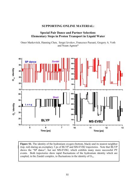
BLYP MS-EVB2

O 1X identity
O 0 identity
60
50
40
30
20
10
60
50
40
30
20
10
SUPPORTING ONLINE MATERIAL:
Special Pair Dance and Partner Selection:
Elementary Steps in Proton Transport in Liquid Water
Omer Markovitch, Hanning Chen, Sergei Izvekov, Francesco Paesani, Gregory A. Voth
and Noam Agmon*
SP dance
L o n g
BLYP
Zundel
Short
5 6
Time [ps]
7
Figure S1. The identity of the hydronium oxygen (bottom, black) and its nearest neighbor
(top, red) during an exemplary 3 ps of BLYP and MS-EVB2 trajectories. Note that BLYP
shows the “SP dance”, but not MS-EVB2, which exhibits many more successful PT
events. Both trajectories show rapid fluctuations of the hydronium identity which are
coupled, in the Zundel complex, to fluctuations in the identity of O1x.
S 1
600
500
400
300
200
100
0
600
500
400
300
200
100
0
MS-EVB2
10 11 12 13
Time [ps]

g i (r)
g i (r)
4
3
2
1
0
4
3
2
1
0
BLYP
MS-EVB2
2.5 3.0 3.5 4.0 4.5 5.0
S 2
r [Å]
g 0
g 1x
g 1yz
Figure S2. Equilibrium O—O radial distribution functions for the hydronium (black)
and its first-shell neighbors (1x − red & 1yz − green) using all time-frames from BLYP
and MS-EVB2 trajectories.

g Short
(r) 0
g Long
(r) 0
4
3
2
1
0
5
4
3
2
1
EVB3
< 5 fs
600 fs
> 500 fs
> 400 fs
> 300 fs
S 3
HCTH
> 726 fs
> 581 fs
> 436 fs
> 218 fs
2.2 2.4 2.6 2.8 3.0
r [Å]
Figure S3. Conditional O—O radial distribution functions for the first solvation layer of
the hydronium for trajectory segments of different lengths (indicated). From the long
segments the first and last 50 fs were deleted. The RDFs for the Long intervals converge
when their length > 300 fs. The RDFs for the Short intervals converge when their length

g 0 (r)
g 0 (r)
g 0 (r)
5
4
3
2
1
0
4
3
2
1
0
4
3
2
1
0
2.5 3.0
r [Å]
S 4
Eq.
Long
Short
f*L + (1-f)*S
BLYP
MS-EVB2
qMS-EVB3
Figure S4. Conditional O—O radial distribution functions for the hydronium using timeframes
from long (blue) and short (cyan) trajectory segments from BLYP, MS-EVB2
and quantal MS-EVB3 trajectories. The yellow line shows a best fit to the equilibrium
RDF (black, Fig. S2) using a linear combination of the two conditional RDFs with a
factor f= 0.74 for BLYP and f=0.77 for MS-EVB2. The fit did not succeed for the qMS-
EVB3 trajectory.

g 1X (r)
g 1X (r)
g 1X (r)
4
3
2
1
0
4
3
2
1
0
4
3
2
1
0
BLYP
MS-EVB2
qMS-EVB3
2.5 3.0
r [Å]
Figure S5. Conditional O—O radial distribution functions for the hydronium nearest
oxygen, O1x, using time-frames from long (blue) and short (cyan) trajectory segments
from BLYP, MS-EVB2 and quantal MS-EVB3 trajectories. The yellow line shows a best
fit to the equilibrium RDF (black, Fig. S2) using a linear combination of the two
conditional RDFs with a factor f= 0.74 For BLYP and f=0.77 for MS-EVB2. The fit did
not succeed for the qMS-EVB3 trajectory.
S 5
Eq.
Long
Short
f*L + (1-f)*S

g (r), |
| δδδδ |
| < ∆
Z
g (r), | δδ
δδ
|
| > ∆
E
4
3
2
1
0
5 Eigen
4
3
2
1
0
EVB3
2.2 2.4 2.6 2.8
r [Å]
Figure S6. The RDFs for Zundel and Eigen cations for various cutoff distances, ∆ (in Ǻ),
in the geometric criterion of Marx et al. [23,41]. Our conditional RDFs for small and
large non-transfer intervals are shown for comparison (black lines). The comparison
shows that the best choice of cut-off distances is ∆Z ≤ 0.1 Ǻ and ∆E = 0.2 Ǻ.
S 6
Zundel
∆ Z =
0.01
0.1
0.2
0.3
0.5
∆
∆
∆ E =
0.5
0.4
0.3
0.2
0.1

g (r)
g (r)
g (r)
g (r)
g (r)
4
2
0
4
2
0
4
2
0
4
2
0
4
2
0
HCTH
+5 fs
−5 fs
−10 fs
−20 fs
−40 fs
2.3 2.4 2.5 2.6 2.7 2.8 2.9 3.0
r [Å]
Figure S7. Time-dependent radial distribution functions for the hydronium [g0(r;t), in brown] and
its nearest oxygen [g1x(r;t), in magenta] just before a proton hopping event in a HCTH simulation.
The dashed and dotted lines show the same RDFs from the ensembles of long (Eigen, blue) and
short (Zundel, cyan) trajectory segments. The larger noise for AIMD trajectories is due to their
limited duration, dictated by their significantly greater computational cost.
S 7
g 0
g 1x
g 0 -Short
g 1x -Short
g0 g1x g0-Long g 1x -Long

g (r)
g (r)
g (r)
g (r)
4
2
0
4
2
0
4
2
0
4
2
4
2
g (r) 0
0
BLYP
2.3 2.4 2.5 2.6 2.7 2.8 2.9 3.0
S 8
+5 fs
−5 fs
−10 fs
−20 fs
−40 fs
r [Å]
g0 g1x g0-Short g 1x -Short
g 0
g 1x
g 0 -Long
g 1x -Long
Figure S8. Same as Figure S5 for an AIMD simulation with the BLYP functional.

g (r)
g (r)
g (r)
g (r)
g (r)
4
2
0
4
2
0
4
2
0
4
2
0
4
2
0
MS-EVB2
2.3 2.4 2.5 2.6 2.7 2.8 2.9 3.0
S 9
+5 fs
−5 fs
−10 fs
−20 fs
−40 fs
r [Å]
Figure S9. Same as Figure S5 for a MS-EVB2 simulation.
g 0
g 1x
g 0 -Short
g 1x -Short
g0 g1x g0-Long g 1x -Long