Wing Kam Liu* and Wei Chen, Northwestern University ... - SAMSI
Wing Kam Liu* and Wei Chen, Northwestern University ... - SAMSI
Wing Kam Liu* and Wei Chen, Northwestern University ... - SAMSI

You also want an ePaper? Increase the reach of your titles
YUMPU automatically turns print PDFs into web optimized ePapers that Google loves.
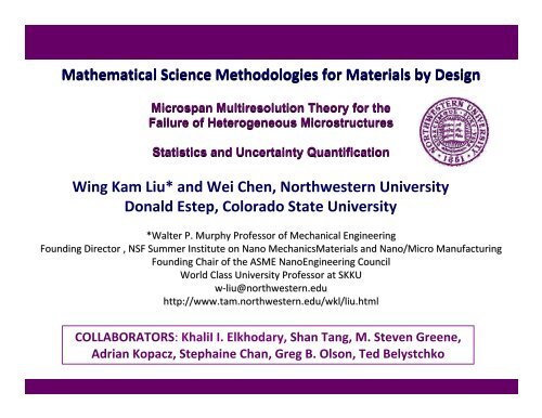
Mathematical Science Methodologies for Materials by Design<br />
Microspan Multiresolution Theory for the<br />
Failure of Heterogeneous Microstructures<br />
Statistics <strong>and</strong> Uncertainty Quantification<br />
<strong>Wing</strong> <strong>Kam</strong> <strong>Liu*</strong> <strong>and</strong> <strong>Wei</strong> <strong>Chen</strong>, <strong>Northwestern</strong> <strong>University</strong><br />
Donald Estep, Colorado State <strong>University</strong><br />
*Walter P. Murphy Professor of Mechanical Engineering<br />
Founding Director , NSF Summer Institute on Nano MechanicsMaterials <strong>and</strong> Nano/Micro Nano/Micro<br />
Manufacturing<br />
Founding Chair of the ASME NanoEngineering Council<br />
World Class <strong>University</strong> Professor at SKKU<br />
w‐liu@northwestern.edu<br />
liu@northwestern.edu<br />
http://www.tam.northwestern.edu/wkl/liu.html<br />
http:// www.tam.northwestern.edu/wkl/liu.html<br />
COLLABORATORS: KhaliI I. Elkhodary, Shan Tang, M. Steven Greene,<br />
Adrian Kopacz, Stephaine Chan, Greg B. Olson, Ted Belystchko
Objectives<br />
Mathematical Science (Multiresolution Mesoscale<br />
Continuum) Methodologies for the Analysis <strong>and</strong> Design of<br />
Multiscale/Multirate Microstructured Materials<br />
•Facilitate the extraction of structure/property/performance<br />
metrics for multiscale/multirate materials design<br />
•Predictive dynamic modeling of fracture nucleation <strong>and</strong><br />
propagation due to contributions from all COUPLED scales<br />
•Set up an approach that is valid across materials systems,<br />
that is MATERIALS GENERIC field equations, <strong>and</strong> MATERIALS SPECIFIC<br />
coupled multiscale constitutive laws<br />
•Uncertainty Sources <strong>and</strong> Quantification<br />
•Wish List for Multiscale Methodologies <strong>and</strong> UQ Discussions Topics
Multiresolution Modeling Scope: Processing/Structure/Property
Mathematical Science Foundation<br />
Mathematically link spatial <strong>and</strong> temporal scales for continuous resolution of a<br />
microstructure<br />
Separate Data by Scales<br />
with Help from<br />
Materials Science<br />
Quantification &<br />
Variability of Data<br />
Sets<br />
Scale 1<br />
Data<br />
Refined<br />
Scale 1<br />
Data<br />
Large Stochastic,<br />
Multi-Scale Data Set<br />
Scale 2<br />
Data<br />
Refined<br />
Scale 2<br />
Data<br />
…<br />
…<br />
…<br />
Scale n<br />
Data<br />
Refined<br />
Scale n<br />
Data
Mathematical Science Foundation, Continued<br />
Reconstruction<br />
of Data Set<br />
Scale linking via testing <strong>and</strong> characterization of samples.<br />
Refined<br />
Scale 1<br />
Data<br />
Scale<br />
Link<br />
Refined<br />
Scale 2<br />
Data<br />
Refined Data in Order of Scale<br />
Refined<br />
Scale n<br />
Data<br />
Keep in mind that the data is in 4D, (x,y,z,t), so the spatial <strong>and</strong> temporal<br />
resolution axes are the 5 th <strong>and</strong> 6 th dimensions. Now the microstructure is<br />
shown in continuous resolution.<br />
To represent the stochastic nature of the data, another dimension will be<br />
added for each parameter with an axis as the variance of that parameter.<br />
…<br />
Scale<br />
Link<br />
Resolution<br />
Axes
Multiresolution Concept<br />
t0<br />
t<br />
f<br />
Macroscale Demonstration<br />
Ice “Reinforced” Ice<br />
Dropped Dropped<br />
Newspaper<br />
Fine resolution<br />
material morphology<br />
Structure dictates the bulk<br />
properties<br />
Properties dictate the bulk<br />
performance
Multiresolution Concept: zoom into a microstructure in the same way that<br />
modern satellite technology allows us to zoom into an image of the earth<br />
a.<br />
Small Number of pixels<br />
per km 2 – suitable for a<br />
global image<br />
TiC<br />
~5 um<br />
0<br />
u<br />
Small Number of<br />
degrees of freedom –<br />
suitable for average<br />
behavior<br />
b.<br />
Increasing Image Resolution<br />
More resolution – cities<br />
can be observed<br />
1<br />
u<br />
Discrete behavior of TiN<br />
primary inclusions<br />
begins to be observed<br />
Increasing Constitutive Resolution<br />
c. d.<br />
Increasing resolution –<br />
buildings can be observed<br />
~1 um ~0.1 um 10 nm<br />
u<br />
Discrete behavior of<br />
TiC secondary<br />
particles is observed<br />
2<br />
<strong>Northwestern</strong> <strong>University</strong><br />
- a fine institution<br />
Macro Micro TiN Sub-Micro TiC Nano<br />
3<br />
u<br />
Very fine resolution – material<br />
interface is observed
Polymer Nanocomposite Material Design<br />
Goals.<br />
(1) Increase transportation materials performance,<br />
(2) ballistic protection, <strong>and</strong><br />
(3) fracture toughness<br />
Atomic bonds visible Aggregated structure,<br />
interface morphology<br />
clear<br />
R<strong>and</strong>om atomic<br />
phase-space<br />
R<strong>and</strong>om secondary<br />
microstructure,<br />
interface morphology<br />
Filler network visible,<br />
detailed shape<br />
information lost<br />
R<strong>and</strong>om aggregation,<br />
mesostructure<br />
Design materials: multiple monomers, fillers, interphase, interface<br />
Filler shape invisible,<br />
statistical homogeneity<br />
R<strong>and</strong>om primary<br />
substructure, statistic<br />
homogeneity<br />
Increasing resolution, decreasing spatial scale, increasing uncertainty<br />
Experiments at various spatial <strong>and</strong> temporal scales <strong>and</strong> its statistical analysis are important<br />
Homogeneous medium<br />
R<strong>and</strong>om operating<br />
conditions<br />
Co-polymer design, interface <strong>and</strong> interphase design, experimental imaging at various scales (V2, V1)<br />
The above is for matrix materials, now we need to add in structural materials to become polymer<br />
matrix composites
High Strength Alloy Analysis & Uncertainty<br />
Goal. Deliver high strength alloys for transportation applications<br />
Primary ( microns) <strong>and</strong> Secondary (tens of nanometers) particles design to control strength & toughness<br />
Quantum-scale design of interfacial strengths between particles <strong>and</strong> matrix<br />
R<strong>and</strong>om operating<br />
(boundary) conditions<br />
TiC<br />
Small Number of degrees<br />
of freedom – suitable for<br />
average behavior<br />
Primary microstructure<br />
r<strong>and</strong>om<br />
~5 μm ~1 μm ~0.1 μm 10 nm<br />
Discrete behavior of TiN<br />
primary inclusions begins<br />
to be observed<br />
Secondary microstructure<br />
r<strong>and</strong>om<br />
Macro Micro TiN Sub-Micro TiC Sub-Nano<br />
Increasing resolution, decreasing spatial scale, increasing uncertainty<br />
Discrete behavior of TiC<br />
secondary particles is<br />
observed<br />
True system size: modeling only 1,000 primary particles, (about 2,500,000) secondary<br />
particles > billions DOFs<br />
Feasible system size: 120 primary particles, >30 million DOF<br />
Destructive evaluation testing dictates the importance of statistical analysis<br />
R<strong>and</strong>om atomic phasespace<br />
Very fine resolution – material<br />
interface is observed
Multiscale Modeling & Simulations<br />
Multiscale Continuum Strata<br />
Computational<br />
Theories<br />
Scale-Bridging Theory<br />
KEY<br />
Control Flow<br />
Information Flow<br />
Atomic<br />
Level<br />
Free<br />
Particle<br />
Dislocation<br />
Walls<br />
Free<br />
Atom<br />
Space‐Time<br />
Discretization<br />
Specimen<br />
Level<br />
interface<br />
Point<br />
Defect<br />
Void<br />
Coalescence<br />
Shear<br />
B<strong>and</strong><br />
interphase Secondary<br />
Phase<br />
Dislocation Ensemble<br />
of Defects<br />
Collective<br />
of Excitation<br />
High Performance<br />
Computing<br />
Uncertainty<br />
Multiresolution Theory<br />
Fields<br />
Rings<br />
Groups
Equations of Archetype Multiresolution Theory<br />
Sets of Equations<br />
(1) Kinematics<br />
(2) Kinetics<br />
(3) Constitutive<br />
(4) Compatibility<br />
(5) Fracture<br />
(6) Uncertainty<br />
materials generic<br />
Multiscale:<br />
Lagrangian,<br />
Computational Theory<br />
materials specific<br />
To be derived for all “building<br />
blocks” as modules in<br />
multiscale framework<br />
Balance<br />
Laws<br />
Reference<br />
Configuration<br />
Constitutive<br />
Laws<br />
Compatibility<br />
Laws<br />
Final<br />
Configuration<br />
Deformation<br />
Crack tip
Microstructural Hierarchy <strong>and</strong> Behavioral Complexity
More on the Theory: Motion Assumptions<br />
Microstructural Kinematics<br />
l*<br />
*<br />
( ( ), , Φ) ≡ ( ( ),0, Φ ) + ∫ ∂α ( ( ), , Φ)<br />
0<br />
x� p ξ l x� p ξ x� p ξ α dα<br />
Beginning from the fundamental theorem of calculus on the second argument…<br />
Meaning of the first term<br />
�x(p(ξ),0,Φ)<br />
Local (intrinsic) point behavior<br />
Meaning of the second term<br />
l*<br />
∫ ∂ x� α ( p( ξ), α, Φ)<br />
dα<br />
0<br />
Corrected influence at p due to<br />
the inhomogeneous neighborhood<br />
x<br />
p
More on Kinematics…<br />
Elemental Kinematics<br />
The effective microstructural rate can be broken down as…<br />
L eff 0 ( p(ξ),x(α ))<br />
( p(ξ)) = Lij + Lij<br />
ij<br />
x(a 1 )<br />
Each term representing<br />
a relative rate for its span<br />
or length scale, hence the<br />
multiscale‐multirate double decomposition<br />
x(0)<br />
( p(ξ),x(α ))<br />
+ Lij x(a 2 )<br />
x(a 1 )<br />
x<br />
( p(ξ),x(α ))<br />
+ ...+ Lij x(a n )<br />
x(a n−1 )<br />
p
More on the Theory: Variational Statement<br />
E� ≡ S L + s L∇ dΩ<br />
∫<br />
1 M M<br />
E� kin =∂ ∫ t ρv<br />
⋅v dΩ<br />
2 Ω<br />
E�= ∫ f ⋅v dΩ<br />
V M<br />
imp i i<br />
Ω<br />
E�= ∫ t ⋅v dΓ<br />
S M<br />
imp i i t<br />
Γ<br />
t<br />
Elemental Kinetics<br />
( M M )<br />
def ij ij ijk ijk<br />
Ω<br />
δE� − δE� = δE�<br />
imp def kin<br />
Elemental Domain ξ<br />
Exp<strong>and</strong>ing V M <strong>and</strong> L M will express all elemental<br />
Fields in terms of microstructural quantities …
More on the Theory: Strong Form<br />
Euler‐Lagrange<br />
Equations<br />
σ −Σ + f = � γ<br />
ij, j ijk , kj i i<br />
Boundary Conditions<br />
Σ ijk n k<br />
= 0<br />
σ ij n j −Σ ijk ,k n j = t i<br />
Discretized Strong Form<br />
δE� − δE� = δE�<br />
imp def kin<br />
[ ]<br />
ρ ρ ρ<br />
S ijk , k − s + B =Γ�ij , for ∀ρ∈ 1,..., n<br />
ij ij<br />
ρ<br />
S ijknk = T ij<br />
for ∀ρ ∈ 1,...,n ⎡⎣ ⎤⎦ Stress conjugate to relative deformation rates<br />
Constitutive laws are needed for all archetypes…<br />
x<br />
p
Three Invariants (Strain rates, Inhomogeneity Length Scales,<br />
Deformation Length Scales) Fracture Space in the Multiscale Context<br />
Maximal stressed zone (m)<br />
Strain rates (s ‐1 )<br />
Materials-Generic Multiresolution Fracture Criterion<br />
10 −2<br />
10 −3<br />
10 −4<br />
10 −5<br />
10 −6<br />
10 −7<br />
10 −8<br />
10 −9<br />
10 −10<br />
10 2<br />
10 3<br />
10 4<br />
10 5<br />
10 6<br />
10 7<br />
10 8<br />
10 1<br />
Local Plastic<br />
Deformation<br />
10 9<br />
Crack tip<br />
Statistical Description<br />
of Structural Inhomogeneity<br />
Structure<br />
Fragmentation<br />
1 st Order Differential Form<br />
Integral Form<br />
(a) (b)<br />
Essential Description<br />
of Structural Inhomogeneity<br />
10<br />
Structural inhomogeneity (m)<br />
−8<br />
10 −7<br />
10 −6<br />
10 −5<br />
10 −4<br />
10 −2 10 −9<br />
10 −3 10 −10<br />
Dimension<br />
(m)<br />
Objects Realizing<br />
Stressed Zone Size<br />
Objects of Structural<br />
Inhomogeneity<br />
10 ‐2 Testing Sample Reinforcement<br />
10 ‐3<br />
10 ‐4<br />
10 ‐5<br />
10 ‐6<br />
Zone at<br />
Impact test<br />
Zone at Fatigue<br />
Fracture Samples<br />
Zone at Cavitation.<br />
Macrocrack<br />
Mechanical Activation<br />
by Processing<br />
10 ‐7 Zone near Crack tip<br />
Coarse Lamellar<br />
Structures. Explosion<br />
Fragments<br />
Coarse Grains<br />
Inclusions<br />
Mn‐Dispersoids in<br />
Aluminum<br />
Al 2 Cu Precipitates<br />
in Aluminum<br />
10 ‐8 Zone at Irradiation Carbides in Steel<br />
10 ‐9<br />
Strain Rate<br />
(s ‐1 )<br />
Crystal Defects.<br />
Nano particles.<br />
Physical<br />
Mechanisms<br />
10 ‐3 Diffusion<br />
10 3 ‐10 6 Wave interactions<br />
10 9<br />
Curl(F M ) = κ<br />
M e p p<br />
*<br />
∫� ( F − R R U ) dx= δ<br />
Shock Waves &<br />
EOS<br />
Atomic lattice<br />
Deformations<br />
Phenomenological<br />
Inhomogeneity<br />
Isothermal shear b<strong>and</strong><br />
Void nucleation & growth<br />
Adiabatic Localization of<br />
shear, Spalling<br />
Fragmentation, Pulverization<br />
(c)
Multiscale Constitutive Physics of Microstructures<br />
Schematic: Complex<br />
Microstructure<br />
(Al - 2139)<br />
Volume Fractions<br />
Phase Spacings<br />
Phase Clusters<br />
Variant Multiplicity<br />
Residual Stresses<br />
Interfaces <strong>and</strong> GBs<br />
Porosities & Defects<br />
Mass Densities<br />
V1<br />
V2<br />
Structure <strong>and</strong> Property Metrics<br />
Edge Crack<br />
Model<br />
Crystallography<br />
� t<br />
� n<br />
� s<br />
Slip System Multiplicity<br />
Habit Planes, Orientations<br />
Deformations<br />
Grain Texture<br />
Elastic/ Plastic Anisotropy<br />
Lattice Curvature<br />
Lattice Stretch, Rotation<br />
Dislocation Densities
Illustrative Example: Two-Scale Elasticity<br />
Dominant Edge Crack<br />
Aluminum Matrix (Usual DOFs)<br />
20% precipitates (Additional DOFs)<br />
Stationary Crack, 5μm× 5 μm,<br />
� ε ε<br />
−1<br />
nom = 20,000 s , nom = 14%<br />
20% Volume fraction of precipitates<br />
Illustration of Design of Materials<br />
Strengthening Mechanisms<br />
(a)Spatial Patterns (Normal Stress)<br />
(b)Magnitudes & Signs (Shear stress)<br />
(c)Curvatures, Nonlocality (Stress couples)<br />
Nanosized<br />
Ω Precipitate<br />
Aluminum<br />
Matrix
Illustrative Example: Two-Scale Elasticity, Continued<br />
S 122(Imbedded Crystal) Σ 122(Matrix Crystal)<br />
[ S, Σ]/<br />
Eb<br />
Stationary Crack, 5μm× 5 μm,<br />
� ε ε<br />
−1<br />
nom = 20,000 s , nom = 14%<br />
Materials Design Implications:<br />
Matrix gradient term (curvature, nonlocality) is important for local fracture processes…<br />
accounts for lattice curvature <strong>and</strong> accommodation processes
Two-Scale Concurrent Multiresolution Model for TiC (Secondary Particles) - Matrix<br />
<strong>and</strong> Direct Numerical Simulation (DNS) of TiN (Primary Particles)<br />
crack<br />
Mod4330 Crack tip specimen #1:<br />
Primary particles (yellow) near crack tip<br />
Reconstruction area: 633x516x259 μm 3<br />
Averaged: 2.857 μm<br />
Spacing: 16 μm<br />
Volume fraction: 1.756%<br />
Ultra High Strength Alloys<br />
Primary Inclusions<br />
Primary Voids<br />
Oxides<br />
Submicron Carbides<br />
Microvoids<br />
Shearing<br />
Mod4330 shear specimen:<br />
Secondary particles (white dots) inside shear b<strong>and</strong><br />
Reconstruction area: 70x15x28μm3 Averaged: 0.117035 μm<br />
Spacing: 2 μm<br />
Volume fraction: 0.0384%<br />
Courtesy of Stephanie Chan (Olson’s group), <strong>and</strong> HJ Jou (QuesTek)<br />
McVeigh & Liu, Linking microstructure & properties through a predictive multiresolution continuum, CMAME, 2008.<br />
McVeigh & Liu, Multiresolution modeling of ductile reinforced brittle composites. J. Mech. Phys. Solids, 2009.<br />
Liu et. al., Complexity science of multiscale materials via stochastic computations, IJNME, 2009.<br />
Tian & Liu et al., “A Multiresolution Continuum Simulation of the Ductile Fracture Process,” JMPS (2010)
Multiscale Materials Modeling, High Performance Alloy<br />
crack<br />
Fracture test<br />
Tomography<br />
Fatigue<br />
crack tip<br />
Mod4330 crack tip specimen #1:<br />
Primary particles (yellow) near crack tip<br />
Reconstruction area: 633x516x259 μm 3<br />
Averaged: 4.857 μm<br />
Spacing: 16 μm<br />
Volume fraction: 1.756%<br />
Fracture Process Model<br />
to be Validated<br />
3μm<br />
Large scale simulations even when blending TiC particles<br />
Degrees of Freedom:<br />
30 million<br />
(132 particles)
Summary:<br />
comparison with experiments<br />
Experiments<br />
Simulation<br />
Pre‐crack<br />
Shear b<strong>and</strong>s<br />
Mixed mode I/II fracture<br />
Primary voids<br />
Crack opening distance along fracture path<br />
Experiments<br />
Simulation<br />
Crack Opening Displacment (μm)<br />
Fracture path<br />
20<br />
15<br />
10<br />
5<br />
0<br />
-5<br />
Fracture path<br />
Experiments<br />
Simulation<br />
0 50 100 150 200 250 300 350<br />
X μm<br />
Experiments<br />
Simulation<br />
Contour plot of crack opening distance<br />
Experiments<br />
Void growth<br />
Simulation<br />
Final void radius (μm)<br />
25<br />
20<br />
15<br />
10<br />
5<br />
Δa<br />
PZ<br />
0<br />
0 1 2 3 4 5 6 7 8 9 10<br />
R0 inclusion radius(μm)
Formation of Multiscale <strong>and</strong> Multistage Fracture Process<br />
Macro deformation (contour of macro effective strain)<br />
(a) Void growth<br />
(primary voids)<br />
Micro deformation (contour of micro effective strain)<br />
(a) Development of<br />
micro deformation<br />
(b) Intense deformation at<br />
ligament between voids<br />
(b) Microvoid sheeting (c) Microvoid shear<br />
coalescence<br />
(c) Initial macro crack (d) Macro crack propagation<br />
Arising from the Strong Interaction between Micro <strong>and</strong> Macro Deformations<br />
(d) Further Microvoid shear<br />
coalescence<br />
I. Multiresolution modeling across multi‐scale of microstructures (voids)<br />
II. Concurrent modeling considering interaction across microstructures has been achieved<br />
(Though there are many primary <strong>and</strong> secondary particles involved)
Animation of the Fracture Process<br />
Initial Fatigue Crack Opening is about 3 microns, a load is<br />
applied gradually until the material reaches the initial <strong>and</strong> then<br />
final fracture toughness strengths followed by unloading to the<br />
final state of deformation<br />
Total experimental time is one minute<br />
The below MOVIE shows the CONCURRENT interaction of macro <strong>and</strong> micro effective<br />
strains due to submicron <strong>and</strong> micron voids growth, interaction, coalescence to form<br />
Micro <strong>and</strong> macro defects (mini-cracks) that eventually define the fracture process zone
Examples of Archetypes <strong>and</strong> their Conformations<br />
ALLOYS POLYMERS CERAMICS<br />
PMC<br />
Multiscale Phenomenology<br />
Shear b<strong>and</strong>ing Pulverization<br />
Cavitation Fragmentation<br />
Conformation of archetypes (sub‐mesoscale)<br />
Sub‐granular structures CNT through Epoxy Resin Polycrystalline Structure Layered Structure<br />
Cortical Bone Lamellae<br />
Archetypes (Space‐filling units)<br />
Crystals<br />
Polymer Chains AlON<br />
CNT MicroCrack<br />
Polymer<br />
Nanocomposite<br />
Fibers<br />
BONES<br />
Collagen Fibrils<br />
Fracture<br />
Path
<strong>Northwestern</strong> <strong>University</strong> Materials Design Loop<br />
METRICS<br />
Structural<br />
Behavioral<br />
Validation<br />
Validation<br />
Concurrent Mesoscale Physics<br />
Multiscale Experiments & Characterization<br />
Multiscale Modeling & Simulation<br />
Scale‐<br />
Bridging<br />
Multiresolution Constitutive Coupling<br />
Direct Numerical Modeling & Simulation<br />
QM<br />
MD<br />
Computational<br />
Theories<br />
Dislocation<br />
Dynamics<br />
Advanced Experiments & Characterization<br />
Sub - mesoscale Physics<br />
High Performance<br />
Computing<br />
Phase<br />
Fields<br />
27
Multiphyics Extensions<br />
Multiresolution<br />
Mesoscale Manifold<br />
Nonlocal<br />
Conformation<br />
Nanomorphic<br />
Archetypes<br />
Blending<br />
Implanting<br />
Cmcm I 4 / mcm I 4m2<br />
Classical Forms Multiresolution<br />
�<br />
( q−p) i∇+<br />
Q = μθ�<br />
� �<br />
pi∇− p+ R= � θ∇iI<br />
Mechanical Balance<br />
Thermal Balance<br />
Electrodynamic Balance<br />
Mass Diffusion Balance<br />
N ⎛ n ⎞ �<br />
⎜q−∑p ⎟i∇+<br />
Q = μθ�<br />
⎝ ⎠<br />
p i∇− p + R = � θ ∇iI<br />
n=<br />
1<br />
� �<br />
n n n n n
Uncertainty Sources <strong>and</strong> Quantification<br />
Inherent structural variation (batch to batch r<strong>and</strong>omness, r<strong>and</strong>om field)<br />
Uncertain multiscale boundary <strong>and</strong> initial conditions<br />
R<strong>and</strong>om parameters determined by experiment or behavior at other scales<br />
Lack of knowledge, lack of information<br />
Low fidelity physical descriptions<br />
Sparse <strong>and</strong> limited experimental data<br />
Missing models <strong>and</strong>/or data for sub-processes<br />
Simulation <strong>and</strong> approximation errors<br />
Discretization <strong>and</strong> finite sampling errors<br />
Solver errors<br />
Statistical modeling <strong>and</strong> representations<br />
Model Complexity<br />
STOCHASTIC PDE’s<br />
Interactions between different sources of errors <strong>and</strong> uncertainty<br />
Uncertainty feedback in coupled processes
General Stochastic Formulation<br />
Write general partial differential equation governing evolution of some<br />
system<br />
( Ωℑ , ,P)<br />
Ω<br />
[ ] ( ,, t ω) [ ] ( ,, t ω)<br />
Tvx + S+ S vx = 0<br />
Temporal operator<br />
( t ω)<br />
[ B+ B ] v x, , = 0<br />
ω<br />
Probability space<br />
Could be infinite dimensional<br />
Governing System of Equations<br />
Boundary condition<br />
( , t = 0, ω) = ( , ω)<br />
v x v x<br />
RANDOM SOLUTION<br />
0<br />
ω<br />
Nominal spatial operator<br />
Initial condition<br />
R<strong>and</strong>om spatial operator<br />
Representations<br />
CDF <strong>and</strong> PDF<br />
Finite collection of samples<br />
Polynomial <strong>and</strong> spectral approximations<br />
Equation Domain<br />
in D( ω ) × (0, T ] ×Ω<br />
Spatial domain<br />
Time domain<br />
R<strong>and</strong>om domain<br />
in ∂ D( ω)<br />
× [0, T]<br />
×Ω<br />
Spatial boundary<br />
in D( ω ) × { t = 0} ×Ω<br />
Uncertainty<br />
(1)<br />
Stochastic differential operators.<br />
R<strong>and</strong>om coefficients<br />
Material properties<br />
Stochastic modeling of<br />
complexity, chaos, fine<br />
(2)<br />
Uncertain environment, i.e. r<strong>and</strong>om<br />
boundary or initial conditions.<br />
Mechanical loads unknown<br />
Temperature field unknown<br />
Current state of system uncertain<br />
(3)<br />
Uncertain domain.<br />
Rough edges from processing<br />
Micro/tele scope finite resolution<br />
Domain manifold subject to stress
Stochastic Mathematical Formulation<br />
General<br />
⎣ Z ⎦<br />
( ,, t )<br />
⎡T+S+ S ⎤v<br />
x Z = 0<br />
in D( ω ) × (0, T ] ×Ω<br />
Solid Mechanics<br />
Uncertainty parameterization technique required<br />
Approximate representations are used<br />
. e.g. KL, PC, finite collection of samples<br />
Dimension reduction methodology<br />
Composition operation<br />
( v) = [ � � � ]( v)<br />
⎡⎣T + S⎤⎦ −T<br />
+ N f g h<br />
[ T ]( • ) = � ∂ ( •)<br />
acceleration t<br />
• = balance law � ∇ ⋅ •<br />
�<br />
[ N ]( ) ( )<br />
[ f ]( •) � constitutive law<br />
[ g](<br />
• ) = objectivity � sym ( •)<br />
[ h](<br />
• ) = compatibility ∇ ( •)<br />
� �<br />
Solution (vector) space<br />
Tensor space<br />
( ,, t )<br />
v x Z<br />
( ,, t )<br />
∇v x Z<br />
Symmetric tensor space<br />
( t )<br />
sym ⎡⎣ ∇v<br />
x, , Z ⎤⎦<br />
Stress tensor space<br />
{ sym ⎡∇ ( , t,<br />
) ⎤}<br />
σ ⎣ v x Z ⎦<br />
Balance Law<br />
acts on stress space<br />
Compatibility<br />
conditions<br />
Objectivity<br />
requirements<br />
Constitutive<br />
law
Stochastic Formulation for Multiresolution Continua<br />
Solid Mechanics<br />
( v) ⎡ + �( ) � � ⎤(<br />
v)<br />
⎡T + S + S ⎤ = −T<br />
N f + f g h<br />
⎣ Z⎦ ⎣ Z ⎦<br />
Intrinsic stress<br />
( )<br />
σ · ∇−Σ: ∇⊗∇ + f = � γ<br />
ρ ρ ρ<br />
S · ∇−s + B = Γ � , ρ = 1, 2, …,<br />
N<br />
Σ · n = 0<br />
σ · n−Σ: ∇⊗n<br />
S<br />
ρ<br />
Macro double stress<br />
Spatial operator<br />
Boundary conditions<br />
( )<br />
body force<br />
= t<br />
· n = T, ρ = 1,2, …,<br />
N<br />
acceleration<br />
Temporal operator<br />
( ( t ) ( t ) ( t ) )<br />
n n n n<br />
σβ , , β = f , f , f sym ∇v x, , Z , L x, , Z −L, ∇L<br />
x, , Z<br />
σ<br />
Z(<br />
s)<br />
x1<br />
β β<br />
R<strong>and</strong>om dimension<br />
Z<br />
x3<br />
Z()<br />
i<br />
t1<br />
x1<br />
VELOCITY<br />
x2<br />
x3<br />
(1)<br />
t1<br />
x2<br />
x1<br />
t2<br />
x3<br />
RANDOM SOLUTIONS<br />
t1<br />
x2<br />
t2<br />
MICRO-VELOCITY GRADIENT<br />
t2<br />
In stochastic collocation, Galerkin<br />
projection, r<strong>and</strong>om dimension<br />
discretized like space <strong>and</strong> time<br />
Constitutive law an implicit function of a denumerable set of r<strong>and</strong>om<br />
variables
Stochastic Constitutive Theory<br />
Denumerable set of r<strong>and</strong>om<br />
variables are structural<br />
descriptors of microstructure<br />
Unique stress distributions<br />
averaged to provide<br />
constitutive behavior<br />
MACRO-SCALE SIMULATION<br />
Greene, M.S., Y. Liu, et al. (2011).<br />
SVE<br />
l<br />
δ =
Stochastic Constitutive Theory<br />
Macroscale, e.g. Fine resolution statistical volume element realizations<br />
d<br />
( , , , T , t, , SA)<br />
〈〉 S = f κ 〈〉〈〉〈 ε ε� 〉 …<br />
( , 〈〉〈〉 , , T , t, , SA,<br />
ω)<br />
S = f κ ε ε� 〈 〉 …<br />
ω<br />
consider statistics of constitutive<br />
behavior other than mean<br />
For multiscale analysis, fine scale simulations create r<strong>and</strong>omness<br />
S<br />
ε<br />
l Realization 1 Realization 2<br />
Deterministic homogenization<br />
(st<strong>and</strong>ard constitutive modeling)<br />
Transfer uncertainty from general<br />
constitutive law to<br />
phenomenological parameters<br />
S<br />
strain<br />
strain rate<br />
temperature<br />
time<br />
structural approx.<br />
ε<br />
General form of stochastic<br />
constitutive theory<br />
Specific form of<br />
S<br />
ε<br />
Realization 3<br />
Fit set of phenomenological<br />
constitutive law parameters to SVE<br />
simulation results<br />
Treat parameters as multivariate<br />
statistical distribution whose data<br />
are each realization<br />
stochastic constitutive theory<br />
Sω = f ⎡⎣Κ( ω),<br />
〈〉〈〉〈 ε , ε� , T〉 , t, …,<br />
SA⎤⎦<br />
Κ( θ ) ~ fK<br />
( κ,<br />
θ )
Desired Features Multiresolution Microspan Theory<br />
• Unifies the three field effects: Nanomorphism, Conformation Complexity, Nonlocality.<br />
• No need for cell modeling, or intermediate models of any kind.<br />
• Strong coupling between length scales <strong>and</strong> 1st <strong>and</strong> 2nd order deformations.<br />
• All archetype formulations are rate-dependent for dynamic applications.<br />
• Conjugate stress measures have clear physical associations (archetype based).<br />
• Asymmetric strain-rate matrices used: Micropolar effects, Interface effect captured<br />
• No requirement on infinitesimality as was in micromorphic theory.<br />
• Nonlocal sweeping permits holonomic velocity fields, simple compatibility conditions<br />
• Derivation of a topologically three-invariant based multiscale fracture theory.<br />
• Higher Order Boundary conditions are easier to interpret (as they are relative)<br />
• No “relative densities” need be defined, so equations are more meaningful.<br />
• No risk of double counting energies<br />
• Continuous formulation, also accepts non-linear spatial fields
Research Challenges/Questions – UQ for Materials<br />
• Materials specific UQ issues<br />
– UQ of Microstructure<br />
– Impact of uncertainty across multiple scales<br />
– Relative role of microstructure <strong>and</strong> property uncertainties<br />
– Life time prediction/extreme events<br />
• General UQ methodologies<br />
– Lack of data/Is extrapolation possible?<br />
– Quantification of material model uncertainty<br />
– Error analysis<br />
• Tradeoffs<br />
– Physics based vs. data-driven model refinement<br />
– Concurrency of material, product, <strong>and</strong> process modeling for design<br />
– When will UQ become intractable?