document - Cosmo

2 Working Group on Numerical Aspects 45
2 Implementation and test of the metric terms
In subroutine explicit horizontal diffusion, the horizontal cartesian terms (a) and (c)
are discretised explicitely whereas the vertical cartesian term (e) is in implicit form to consider
the fact that the stability criterion can be violated in the case of small vertical level
distance or large diffusion coefficients. The metric terms (b) and (d) are some sort of horizontal
correction due to the terrain following coordinate system and therefore the first attempt
for their discretisation is also in explicit form.
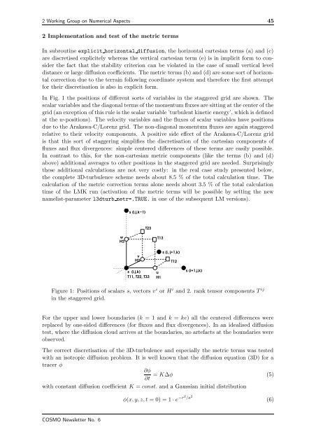
In Fig. 1 the positions of different sorts of variables in the staggered grid are shown. The
scalar variables and the diagonal terms of the momentum fluxes are sitting at the center of the
grid (an exception of this rule is the scalar variable ’turbulent kinetic energy’, which is defined
at the w-positions). The velocity variables and the fluxes of scalar variables have positions
due to the Arakawa-C/Lorenz grid. The non-diagonal momentum fluxes are again staggered
relative to their velocity components. A positive side effect of the Arakawa-C/Lorenz grid
is that this sort of staggering simplifies the discretisation of the cartesian components of
fluxes and flux divergences: simple centered differences of these terms are easily possible.
In contrast to this, for the non-cartesian metric components (like the terms (b) and (d)
above) additional averages to other positions in the staggered grid are needed. Surprisingly
these additional calculations are not very costly: in the real case study presented below,
the complete 3D-turbulence scheme needs about 8.5 % of the total calculation time. The
calculation of the metric correction terms alone needs about 3.5 % of the total calculation
time of the LMK run (activation of the metric terms will be possible by setting the new
namelist-parameter l3dturb metr=.TRUE. in one of the subsequent LM versions).
w
H3
s (i,j,k−1)
v
H2
T23
s (i,j,k)
T11, T22, T33
T13
u
H1
s (i, j+1,k)
T12
s (i+1,j,k)
Figure 1: Positions of scalars s, vectors v i or H i and 2. rank tensor components T ij
in the staggered grid.
For the upper and lower boundaries (k = 1 and k = ke) all the centered differences were
replaced by one-sided differences (for fluxes and flux divergences). In an idealised diffusion
test, where the diffusion cloud arrives at the boundaries, no artefacts at the boundaries were
observed.
The correct discretisation of the 3D-turbulence and especially the metric terms was tested
with an isotropic diffusion problem. It is well known that the diffusion equation (3D) for a
tracer φ
∂φ
= K∆φ (5)
∂t
with constant diffusion coefficient K = const. and a Gaussian initial distribution
COSMO Newsletter No. 6
φ(x, y, z, t = 0) = 1 · e −r2 /a 2
(6)