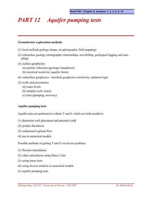
PART 12 Aquifer pumping tests - Dr. M. Zreda - University of Arizona

PART 12 Aquifer pumping tests 

Groundwater exploration methods 

(1) local surficial geology (maps, air photographs, field mapping) 

(2) subsurface geology (stratigraphic relationships, test-drilling, geological logging and sampling) 

(3) surface geophysics 

(a) seismic refraction (geologic boundaries) 

(b) electrical resistivity (aquifer limits) 

(4) subsurface geophysics - borehole geophysics (resistivity, radiation logs) 

(5) wells and piezometers 

(a) water levels 

(b) samples (soil, water) 

(c) tests (pumping, recovery) 

Aquifer pumping tests 

Aquifer tests are performed to obtain T and S, which are both needed to 

(1) determine well placement and potential yield 

(2) predict drawdown 

(3) understand regional flow 

(4) put in numerical models 

Possible methods of getting T and S via inverse problem: 

(1) flownet calculations 

(2) other calculations using Darcy’s law 

(3) using tracer tests 

(4) using inverse solution in numerical models 

(5) aquifer pumping tests 

Read F&C: Chapter 8, sections 1, 2, 3, 5, 6, 10 

Hydrogeology, 431/531 - University of Arizona - Fall 2007 Dr. Marek Zreda

Aquifer pumping tests 88 

Assumptions: 

Steady state pumping test 

(1) Homogeneous, isotropic, confined aquifer with steady flow, 3-D 

(2) Horizontal flow: 3-D changes to 2-D 

(3) Impervious top and bottom and constant aquifer thickness b 

(4) Prescribed head boundary around the well, i.e., “well on an island” setting. Water comes from 

a lateral boundary only (Theis assumption). 

(5) Radial 1-D flow towards the well 

(6) Well fully penetrates (compare to assumption 2); if not, then we will have vertical component 

(7) Well pumps at a constant rate Q; Q appears as a boundary condition 

PDE: 

∇ xy 

∇ h 2 = 0 in 3-D 

2 

h = 0 or 

x 2 

∂ h 

∂ y 2 

∂ h 

+ = 0 

∂ 

1 

-- 

∂ ⎛ ∂h 

r-----⎞ = 0 Laplace equation for radial flow 

r ∂r⎝ 

∂r⎠ 

= 

;;;; 

;;;; yyyy ;;;; yyyy 

yyyyh 

h = H 

lake lake 

1 

-- 

∂ ⎛ ∂h 

r-----⎞ = 

0 

r ∂r⎝ 

∂r⎠ 

h 2 

r 2 

h 1 

r 1 

Q 

R 

b 

Hydrogeology, 431/531 - University of Arizona - Fall 2007 Dr. Marek Zreda 

2 

2 

H 

q increases close to the well. Why?


Boundary conditions: 

BC1: Prescribed head at the lake: 

h = H at r = R 

BC2: Prescribed flux at the well (= pumping rate Q): 

Q = K(2πrb)(∂h/∂r) at r = r w (well radius) 

or, after rearranging and putting T = Kb: 

--------- 

Q 

r 

2πT 

h ∂ 

= ----- 

∂r 

Solution: 

Integrate once: 

Use BC2: C 1 = Q/(2πT) 

Rearrange by grouping r terms together 

Integrate 

Use BC1: 

r h ∂ 

----- = C1 ∂r 

∂r 

∂h = C1---- r 

Q 

h = C1lnr + C2 = --------- lnr + C2 2πT 

C 2 

Q 

= H – --------- lnR 

2πT 

Final solution for h becomes 

h – H 

--------- 

Q r 

= 

⎛ln- ⎞ 

2πT ⎝ R⎠ 

Thiem equation 



For two observation wells (h 1 and h 2 in the figure above): 

Graphically, the solution is 

s = drawdown = s(r) 

at r = R, s = 0 (no drawdown at the lake) 

Suppose r1 = rw r2 = R 

then 

h2 – 

h 1 

--------- 

Q r2 = ⎛ln-- ⎞ 

2πT ⎝ ⎠ 

H 

h 2 

h 

s 2 

r 2 

r 1 

on normal paper 

h1 = hw h2 = H 

H – hw Q 

--------- 

2πT 

R 

= ln---- = sw Knowing Q, T, R - can calculate drawdown 

r w 

r 

Having observation wells is advantageous because we then know drawdowns and can get T of the 

aquifer: 

T 

------------ 

Q R 

= ln----- 

Thiem equation 

2πs w 

r w 

In practice, there is no constant R where the head is H. Instead, R depends on Q, and this formula 

does not work. Two observation wells are thus necessary to solve for T 


h 

on semilog paper 

straight line 

Q r2 T = 

------------------------ ln--- 

Thiem equation for observation wels 

( – ) r1 2π h 2 h 1 

log r


Rewrite in terms of decimal logarithms (log) 

T 

2.3Q r2 = -----------------------log--- Thiem equation for observation wells 

2π( h2 – h1) r1 and if r 2 = 10r 1 , log10 = 1 and we have 

T 

= 

------------- 

2.3Q 

Equilibrium (= Thiem) steady state equation 

2π∆h 

This is usually used for more than two observation wells. 

If aquifer is infinite (no lakes) and confined, supply of water is from storage → transient flow. 

;;;; 

;;;; yyyy ;;;; yyyy 

Q 

= h0 at r = infinity for all t 

yyyyh 



Transient pumping test 

Consider an aquifer with following assumptions: 

PDE 

• homogeneous and isotropic medium 

• horizontal, radial, 1-D flow 

• confined horizontal aquifer with constant thickness 

• no leakage (i.e., impervious top and bottom) 

• water released from storage instantaneously 

• small well diameter (no storage in well) 

• constant pumping rate Q 

• infinite lateral extent of aquifer 

• Darcy’s law valid 

• saturated (single-phase) flow 

• homogeneous fluid 

• isothermal conditions 

∇ h 2 

in radial coordinates 

or, in terms of drawdown (s), using the relationship ∂h/∂r = - ∂s/∂r 

Boundary conditions 

Initial condition 

S 

-- 

T 

h ∂ 

= ----- h=h(x, y, t) 

∂t 

1 ∂ 

-- ⎛ ∂h 

r-----⎞ S 

-- 

r ∂r⎝ 

∂r⎠ 

T 

h ∂ 

= ----- h=h(r, t) 

∂t 

1 ∂ 

-- ⎛ ∂s 

r---- ⎞ S 

-- 

r ∂r⎝ 

∂r⎠ 

T 

h ∂ 

= ----- h=h(r, t) (1) 

∂t 

BC1: s = 0 @ r = ∞ 

BC1: 

Q 

--------- r 

2πT 

s ∂ 

= – lim ⎛ ---- ⎞ 

⎝ ∂r⎠ 

r → 0 

IC: s = 

0 @ t = 0 for all r 



The solution of equation 1 is (Theis, 1935) 

where u defined as 

is called similarity variable, and W(u) is called Theis well function in hydrology (tabulated in 

hydrogeology books; for example on p. 318 of Freeze and Cherry) or exponential integral in 

mathematics (tabulated in mathematics books). The exponential integral is calculated as 

where γ = 0.57721566..... is the Euler's number 

s 

∞ 

u 

e – 

Q 

= --------- ------ du 

= 

4πT u 

∫ 

u 

u 

= 

Wu ( ) = – lnu – γ – 

r 2 ------- 

S 

4Tt 

∞ 

∑ 

k = 1 

---------W 

Q 

( u) 

4πT 

Plot the solution on a log-log graph (this is the Theis type curve; left panel below). If Q, T and S 

are known, s(r, t) can be calculated and plotted on a log-log graph (these are the pumping test 

data; right panel below). Note that the shapes of the two graphs, W(u) vs. u and s vs. t, are the 

same. We can, therefore, use them together to determine S and T. The procedure used is called the 

curve matching method. 

log W(u) Theis type curve 

log 1/u 


u k 

------ ( – 1) 

kk! 

k 

log s Pumping test data 

log t


Curve matching method (Theis method) 

Can get T and S if Q is known and h is measured in time. 

Procedure: 

(1) Plot W(u) vs. 1/u on a log-log graph. 

(2) Plot test data (s vs. t) on the same size graph. 

(3) Overlay the graphs so that the curves are on top of each other. 

(4) Pick any point in the common area. 

(5) For this point, read off the following values: 1/u and W(u) for the first graph, and t and s from 

the second graph. 

(6) Calculate the transmissivity using 

T 

= 

Q 

--------W( u) 

4πs 

(7) Calculate the storativity using 

4Tt 

S 

r 2 

= 

------- u 



Jacob logarithmic approximation 

For large t, u = r 2 S/4Tt becomes small. For u


Plot on semi-log graph. 

Late-time data (large t) should form a 

straight line. Note, however, that early-time 

data (small t) are off the straight line because 

these small t values do not make u sufficiently 

small and the Jacob method cannot 

be applied for these data. 

Change to decimal log 

For one log cycle, we have log(t 2 /t 1 ) = log 10 = 1, and the solution for T is 

Because we know the intercept (at s = 0), we can also calculate the storativity S: 

at s = 0 we have t = t 0 and we have 

which is true only if 

true only if 

so 

s 

0 

∆s 

T 

2.3Q t2 = ----------log--- 4πT t1 = 

------------ 

2.3Q 

4π∆s 

2.3Q 

----------- 

2.25Tt 

4πT r 2 = log--------------- S 

2.25Tt 0 

2.3Q 

----------- 

4πT r 2 = log----------------- S 

2.25Tt 0 

r 2 log----------------- = 0 

S 

2.25Tt 0 

r 2 ----------------- = 1 

S 

S = 

2.25Tt0 r 2 

----------------- 


s 

t 0 

s 

log t 

Q 

--------- 

2.25Tt 

4πT r 2 = ln--------------- S


When is u sufficiently small to use the Jacob logarithmic approximation? 

Look at u = r 2 S/4Tt and note that 

(1) u ∝ r 2 ⇒ small r or long t needed 

(2) u ∝ S ⇒ confined aquifer better; if unconfined then need long t 

(3) u ∝ 1/t ⇒ long time always good 

(4) u ∝ 1/T ⇒ large T good; if small T then need long t 

In summary, long t is always good. 

Distance-drawdown data 

At two or more observation wells at the same time: 

Let observation wells be: s(r 1 ) = s 1 and s(r 2 ) = s 2 , and r 2 > r 1 (i.e., also s 2 < s 1 ). 

Let 

s 

Q 2.25Tt 

--------- 

4πT r 2 = ln --------------- Jacob approximation 

S 

∆h = s1– s2 = 

∆h 

Q 

--------- 

4πT 

2.25Tt 2.25Tt 

ln--------------- 

– ln--------------- 2 2 

r1S r2S Q 

--------- ⎛ 

r2 --- ⎞ 

4πT ⎝r⎠ 1 

2 

= ln 

Q r2 ∆h = 

--------- ln ---- Thiem equation ! 

2πT r1 (Note that although this is not steady-state flow, Thiem equation works, by accident). 



Can be used for linear systems only. 

Linear are: 

• confined aquifer 

Non-linear are: 

Principle of superposition 

• phreatic aquifer (because T = T(h)) 

• vadose zone (because of multiphase flow) 

Drawdowns calculated for multiple wells located in different places or drawdowns calculated for 

the same well that has variable pumping rate at different times can be linearly added. 

It means that we can calculate drawdown for each well separately and then add them to get total 

drawdown. 

Superposition in space: 2 wells pumping at the same time t 

Superposition in time: 1 well; start at rate Q1 at time t1; switch to rate Q2 at time t2 

Q2 

Q1 

Q 

s 

s1 

t1 t2 

total s 


s2 

t


Case 1: Constant head boundary (river) 

To do the calculations of 

drawdown, we replace the 

real well-river system with 

the equivalent system that 

consists of the same real well 

(left side in the figure below) 

and an injecting image well 

(right side, on the other side 

of the boundary, at the same 

distance from the boundary 

as the real well). The injecting 

image well simulates the 

boundary (its effect on head 

and drawdown is exactly the 

same as the effect of the 

river). The figure below 

shows the distribution of 

drawdown in this system. 

Boundary effects 

Note that drawdown is zero 

along the river (this is expected because the river 

is a constant head boundary). We demonstrate 

this mathematically by calculating total drawdown 

as follows: 

Total: 

s r 

s i 

--------- 

Q 2.25Tt 

= ln--------------- 

4πT 2 

S 

r r 

--------- 

– Q 2.25Tt 

= ln--------------- 4πT 2 

S 

ri rr r i 

Y Data 

40 

35 

30 

25 

20 

15 

10 

5 

0 

-2 

0 5 10 15 20 25 30 35 40 

X Data 


-2 

-4 

-2 

-2 

Qr 

real well 

(discharge) 

Q 

s = --------ln--- = 

0 because at the boundary rr = ri 2πT 

rr 

0 

0 

0 

0 

M 

ri 

2 

4 

2 

2 

2 

Qi = -Qr 

image well 

(recharge)


Case 2: No-flow (barrier) boundary (need zero gradient at boundary) 

We replace the barrier with an image pumping 

well (pumping at the same rate as the real pumping 

well). 

Because we have two pumping wells, they produce 

big drawdown. Will never reach steady 

state. 

Drawdown is calculated by superposition: 

s r 

s i 

Q 

= --------- ln--------------- 2.25Tt 

4πT 2 

S 

Q. How to demonstrate that this is a no-flow boundary? 

r r 

Q 

= --------- ln 

2.25Tt 

--------------- 

4πT 2 

S 

r i 

Q 

s --------- 

2.25Tt 

= 

ln--------------- 

2πT rrr iS A. Derive an expression for gradient and show that the gradient in the direction normal to the 

boundary is zero at the boundary. 


Qr 

real well 

(discharge) 

rr 

M 

ri 

Qi = Qr 

image well 

(discharge)


Effects of boundaries on Theis and Jacob plots 

log drawdown 

drawdown 

ideal Jacob response 

Impermeable boundary 

log time 

log time 

impermeable boundary 

(slope is doubled) 

Ideal type curve 

Recharge boundary 

recharge boundary 



Phreatic aquifer 

Initially, the aquifer 

behaves like a confined 

aquifer (Ss 

only). Then, the signal 

propagates and 

pore drainage occurs 

(Sy). 

Leakage 

No leakage before pumping (two 

aquifers in equilibrium). Neglect 

storage in aquitard. 

Actual drawdown is horizontal for 

large t because there is steady state 

solution for leaky systems (there is 

additional source of water, much 

like in the case of a constant head 

boundary). It is achieved sooner in 

observation wells closer to the 

pumping well. 

Other variations in drawdown shapes 

s 

early 

time 

s 

Ss only 

no leakage 

Sy only 


late 

time 

actual 

drawdown 

actual 

drawdown 

log t 

log t


Partial penetration 

We have 3-D flow due to partial 

penetration. 

If s = const, partially penetrating 

wells give less Q than fully penetrating 

wells because more energy 

is required to get water up (less 

area?). 

If Q = const, partially penetrating 

well causes more drawdown than 

does fully penetrating one. 

Drawdown curve far away from s 

the pumping well looks like fully 

penetrating and the slope of drawdown curve approaches slope of fully penetrating well drawdown. 

Penetration is important in calculating S. Do not use the late curve (straight line); use the early 

one. 

Large diameter well 

Has storage, usually built in low-K 

aquifers. Specific yield of the 

well: S y = 1. S is overestimated 

(t 1 ). Use t 0 to get S. 

s 

t 0 

wrong 

estimation 

of S 

actual 

drawdown 

fully 

penetrating 


t 1 

small 

diameter 

well 

t 0 

use this to get S 

large 

diameter 

well 

log t 

log t


Skin and well screen effect 

Mud sealing the well forms “skin” 

reducing K around the well bore. 

If well screened in gravel, K is 

increased around the well. 

S is underestimated! 

For given Q, more drawdown for 

skin well, but slope the same for 

both. Reason: greater gradient is 

necessary for water to flow to the 

well. 

s 

skin 

effect 

no skin 

(ideal well) 


log t

PART 12 Aquifer pumping tests - Dr. M. Zreda - University of Arizona

Create successful ePaper yourself

Delete template?

Save as template?