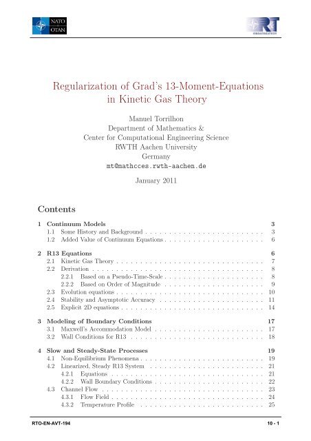
Regularization of Grad's 13-Moment-Equations in Kinetic Gas Theory

Re g u la riz a tio n o f Gra d ’s 1 3 -Mo m e nt-Equ a tio n s
in K in e tic Ga s Th e o ry
Contents
Manuel Torrilhon
Department of Mathematics &
Center for Computational Engineering Science
RWTH Aachen University
Germany
mt@mathcces.rwth-aachen.de
January 2011
1 Continuum Models 3
1.1 Some History and Background . . . . . . . . . . . . . . . . . . . . . . . . . 3
1.2 Added Value of Continuum Equations . . . . . . . . . . . . . . . . . . . . . 6
2 R13 Equations 6
2.1 Kinetic Gas Theory . . . . . . . . . . . . . . . . . . . . . . . . . . . . . . . 7
2.2 Derivation . . . . . . . . . . . . . . . . . . . . . . . . . . . . . . . . . . . . 8
2.2.1 Based on a Pseudo-Time-Scale . . . . . . . . . . . . . . . . . . . . . 8
2.2.2 Based on Order of Magnitude . . . . . . . . . . . . . . . . . . . . . 9
2.3 Evolution equations . . . . . . . . . . . . . . . . . . . . . . . . . . . . . . . 10
2.4 Stability and Asymptotic Accuracy . . . . . . . . . . . . . . . . . . . . . . 11
2.5 Explicit 2D equations . . . . . . . . . . . . . . . . . . . . . . . . . . . . . . 14
3 Modeling of Boundary Conditions 17
3.1 Maxwell’s Accommodation Model . . . . . . . . . . . . . . . . . . . . . . . 17
3.2 Wall Conditions for R13 . . . . . . . . . . . . . . . . . . . . . . . . . . . . 18
4 Slow and Steady-State Processes 19
4.1 Non-Equilibrium Phenomena . . . . . . . . . . . . . . . . . . . . . . . . . . 19
4.2 Linearized, Steady R13 System . . . . . . . . . . . . . . . . . . . . . . . . 21
4.2.1 Equations . . . . . . . . . . . . . . . . . . . . . . . . . . . . . . . . 21
4.2.2 Wall Boundary Conditions . . . . . . . . . . . . . . . . . . . . . . . 22
4.3 Channel Flow . . . . . . . . . . . . . . . . . . . . . . . . . . . . . . . . . . 23
4.3.1 Flow Field . . . . . . . . . . . . . . . . . . . . . . . . . . . . . . . . 24
4.3.2 Temperature Profile . . . . . . . . . . . . . . . . . . . . . . . . . . 25
RTO-EN-AVT-194 10 - 1

CONTENTS CONTENTS
4.3.3 Full Simulation . . . . . . . . . . . . . . . . . . . . . . . . . . . . . 26
4.4 Flow Around a Sphere . . . . . . . . . . . . . . . . . . . . . . . . . . . . . 28
4.4.1 Analytic Solution . . . . . . . . . . . . . . . . . . . . . . . . . . . . 28
4.4.2 Stream and Heat Lines . . . . . . . . . . . . . . . . . . . . . . . . . 31
5 Nonlinear Problems 32
5.1 Shock Profiles . . . . . . . . . . . . . . . . . . . . . . . . . . . . . . . . . . 32
5.2 Multi-Dimensional Shock Simulation . . . . . . . . . . . . . . . . . . . . . 35
5.3 Hyperbolicity . . . . . . . . . . . . . . . . . . . . . . . . . . . . . . . . . . 36
5.3.1 Speed of propagation . . . . . . . . . . . . . . . . . . . . . . . . . . 37
5.3.2 Loss of Hyperbolicity . . . . . . . . . . . . . . . . . . . . . . . . . . 38
5.3.3 Pearson Closure . . . . . . . . . . . . . . . . . . . . . . . . . . . . . 40
6 Further Reading 42
10 - 2 RTO-EN-AVT-194

1 Continuum Models
1 CONTINUUM MODELS
The accurate modeling and simulation of non-equilibrium processes in rarefied fluids or
micro-flows is one of the main challenges in present fluid mechanics. The traditional
models developed centuries ago are known to loose their validity in extreme physical situations.
In these classical models the non-equilibrium variables, stress and heat flux, are
coupled to gradients of velocity and temperature as given in the constitutive relations of
Navier-Stokes and Fourier (NSF). These relations are valid close to equilibrium, however,
in rarefied fluids or micro-flows the particle collisions are insufficient to maintain equilibrium.
Away from equilibrium the inertia and higher order multi-scale relaxation in the
fluid become dominant and essential.
1.1 Some History and Background
It is generally accepted that kinetic theory based on a statistical description of the gas
provides a valid framework to describe processes in a rarefied regime or at small scales.
Introductions into kinetic theory and its core, Boltzmann equation, can be found in many
text books like Cercignani (1988), Cercignani (2000), Chapman and Cowling (1970) or
Vincenti and Kruger (1965). The main variable used to describe the gas is the distribution
function or probability density of the particle velocities which describes the number density
of particles with certain velocity in each space point at a certain time. However, in
many situations this detailed statistical approach yields a far too complex description
of the gas. It turns out to be desirable to have a continuum model based on partial
differential equations for the fluid mechanical field variables. This model should accurately
approximate the multi-scale phenomena present in kinetic gas theory in a stable and
compact system of field equations.
The main scaling parameter in kinetic theory is the Knudsen number Kn. It is computed
from the ratio of the mean free path between collisions λ and a macroscopic length
L, such that Kn = λ/L. Complete equilibrium is given for Kn = 0, described by the
dissipationless Euler equations. In many processes gas dynamics with Navier-Stokes and
Fourier fail at Kn ≈ 0.01 and sometimes even for smaller values. Some examples will
be discussed in this notes. The range of the Knudsen number is shown in Fig.1. Similar
diagrams can be found in many other texts, for example in Karniadakis and Beskok
(2001). The numbers are only for orientation and may depend on the process at hand and
also on the philosophy of the respective scientist. Depending on the focus of the process
Navier-Stokes-Fourier can be used up to a Knudsen number between 10 −2 and 10 −1 . On
the other hand, for large Knudsen numbers the collisions between the particles can be
neglected and they move ballistically in a free flight.
The range between these limiting cases can be split into two parts. One part is the
kinetic regime in which the non-equilibrium is so strong that a detailed description by a
distribution function becomes necessary. In this regime either the Boltzmann equation
is solved directly or the direct simulation Monte-Carlo (DSMC) method is employed, see
Bird (1998). The other part is the so-called transition regime where a fluid description
is still possible, although a larger set of field variables and/or higher derivatives may be
needed. In this regime Boltzmann simulations or DSMC become increasingly expensive.
The limit for the continuum models is currently around Kn = 1, depending on the process.
RTO-EN-AVT-194 10 - 3

1 CONTINUUM MODELS 1.1 Some History and Background
The aim of the research is to establish continuum models and to push their limit further.
The transition regime is typically split further into a slip regime at lower Knudsen number.
However, we will see below that with the relevance of slip also bulk effects occur that can
not be described by advanced boundary modeling only.
There exist two classical approaches to the transition regime. Close to the limit
Kn → 0 an asymptotic analysis in powers of the Knudsen number, called Chapman-
Enskog expansion, leads in first order to the classical NSF relations including specific
expressions of the transport coefficients, see the textbook Chapman and Cowling (1970).
The Chapman-Enskog expansion can be used to derive higher order constitutive relations
from the Boltzmann equation. The resulting equations are called Burnett equations for
the second order and super-Burnett in case of third order. They include ever higher
gradients of temperature and velocity into the constitutive relations for stress and heat
flux. The relations of super-Burnett order for the full Boltzmann equation are already
forbiddingly complex and even higher order was never considered. Furthermore, in general
the corrections of higher than first order, i.e., Burnett and super-Burnett relations, are
known to be unstable, as shown by Bobylev (1982). In special cases the Burnett equations
have been used to calculate higher Knudsen number flow, for example by Agarwal et al.
(2001), Lockerby and Reese (2003), or Xu and Li (2004). In some cases the instability of
Burnett equations could be overcome by ad-hoc modifications as in Zhong et al. (1993)or
in Xu (2002). However, general stable Burnett relations that follow rigorously from the
Boltzmann equation seem not to exist.
An alternative approximation strategy in kinetic theory is given by Grad’s moment
method based on Hilbert expansion of the distribution function in Hermite polynomials.
The method is described in Grad (1949) and Grad (1958). In contrast to Chapman-Enskog
and Burnett this method extends the set of variables of a possible continuum model
beyond the fields of density, velocity and temperature. The additional variables are given
by higher moments of the distribution function. The 13-moment-case of Grad considers
evolution equations for density, velocity and temperature and stress tensor and heat
flux. Higher moment theories include more moments which lack physical intuition. In the
context of phenomenological thermodynamics extended theories proved to be successful
in many test cases, see the text book Müller and Ruggeri (1998) or, e.g., Jou et al. (1996).
Both approaches, Chapman-Enskog and Grad, are explained in detail elsewhere in this
book.
Large moment systems based on Grad’s approach with hundreds of variables where
used to describe shock structures, see the dissertation of Au (2001), the shock-tube experiment
in the work Au et al. (2001), and heat conduction in Struchtrup (2002). A
computationally efficient approach to large moment systems is using comulant theory, see
Seeger and Hoffmann (2000). However, even though the capability of Grad’s moment
method is assured by these results, its usefulness is restricted due to slow convergence.
Indeed, many moments are needed to describe high non-equilibrium which results in large
systems of partial differential equations to be solved.
Moment systems provide a rich mathematical structure like hyperbolicity and entropy
law discussed, e.g., in Müller and Ruggeri (1998) and in Levermore (1996). It has been
argued that evolution equations in physics should always be hyperbolic in order to provide
a finite speed of propagation. When using a nonlinear extension of Grad’s approach based
on the maximum-entropy-principle as in Müller and Ruggeri (1998) and Levermore (1996),
10 - 4 RTO-EN-AVT-194

1.1 Some History and Background 1 CONTINUUM MODELS
Euler Eqn
½
½
NSF Eqn
transition
regime kinetic regime free flight
10 ¡2
10 ¡1
equilibrium non-equilibrium
! !
½
! !
½
1.0 10.0
Kn
½
Figure 1: Overview of the range of Knudsen number and various model regimes.
the moment systems lead to stable hyperbolic equations. However, in practical explicit
systems hyperbolicity is given only in a finite range due to linearization. In Junk (1998)
and Junk (2002) it is shown that the fully nonlinear maximum-entropy approach has
sever drawbacks and singularities. Furthermore, the hyperbolicity leads to discontinuous
sub-shock solutions in the shock profile. A variant of the moment method has been
proposed by Eu (1980) and is used, e.g., in Myong (2001). Recently, a maximum-entropy
10-moment system has been used by Suzuki and van Leer (2005).
Both fundamental approaches of kinetic theory, Chapman-Enskog and Grad, exhibit
severe disadvantages. Higher order Chapman-Enskog expansions are unstable and Grad’s
method introduces subshocks and show slow convergence. It seems to be desirable to
combine both methods in order to remedy their disadvantages. Such an hybrid approach
have already been discussed by Grad in a side note in Grad (1958). He derives a variant
of the regularized 13-moment equations given below, but surprisingly he neither gives any
details nor is he using or investigating the equations. In the last fifty years the paper Grad
(1958) was cited as standard source for introduction into kinetic theory, but, apparently,
this specific idea got entirely lost and seems not to be known in present day literature.
The Chapman-Enskog expansion is based on equilibrium and the corrections describe
the non-equilibrium perturbation. A hybrid version which uses a non-equilibrium as basis
is discussed in Karlin et al. (1998). They deduced linearized equations with unspecified
coefficients. Starting from Burnett equations Jin and Slemrod (2001) derived an extended
system of evolution equations which resembles the regularized 13-moment system. It is
solved numerically in Jin et al. (2002). However, the tensorial structure of their relations
is not in accordance with Boltzmann’s equation. Starting from higher moment systems
Müller et al. (2003) discussed a parabolization which includes higher order expressions
into hyperbolic equations.
The regularized 13-moment-equations presented below were rigorously derived from
Boltzmann’s equation in Struchtrup and Torrilhon (2003). The key ingredient is a Chapman-
Enskog expansion around a pseudo-equilibrium which is given by the constitutive relations
of Grad for stress tensor and heat flux. The final system consists of evolution equations
for the fluid fields: density, velocity, temperature, stress tensor and heat flux. The closure
procedure adds second order derivatives to Grad’s evolution equations of stress and heat
flux, thus regularizes the former hyperbolic equations into a mixed hyperbolic-parabolic
system with relaxation. The relaxational and parabolic part is only present in the equations
of stress and heat flux and models the multi-scale dissipation of Boltzmann’s equation,
see Struchtrup and Torrilhon (2003). Like the Boltzmann equation the R13 system
is derived for monatomic gases and all the results in this chapter are restricted to this
case. The extension to poly-atomic gases or mixtures is future work. The text book by
Struchtrup (2005b) provides an introduction to approximation methods in kinetic theory
RTO-EN-AVT-194 10 - 5

2 R13 EQUATIONS 1.2 Added Value of Continuum Equations
including the regularized moment equations. However, recent developments on boundary
conditions and boundary value problems are not covered.
1.2 Added Value of Continuum Equations
Predictive simulations of non-equilibrium flows of gases in rarefied regimes of micro-scale
situations are important for many technical applications. Direct solutions of Boltzmann’s
equation or the stochastic particle method (DSMC) give very accurate results in principle
for the whole range of the Knudsen number. However, computational expense remains
a major drawback and is considered as an important argument for the use of continuum
models in the transition regime. However, there is another interesting fact that is often
underestimated. Non-equilibrium flows exhibit behavior which is in contrast to the
intuition of fluid dynamics and difficult to understand. The simulations of Boltzmann
and DSMC may give accurate predictions of this behavior but it is important to realize
that their results actually do not easily provide a detailed physical understanding of the
process.
The reason is that our understanding of physical phenomena is very often based on
the structure and qualitative behavior of differential equations and their solutions. Many
aspect of fluid dynamics like convection, viscosity, heat conduction are closely linked to
particular aspects of the differential equations describing the flow. Our understanding of
these phenomena arise from analytical solutions for small models that display how the
coupling of the mathematical terms influence the behavior of the solution, which is then
directly (and sometimes too quickly) translated into reality.
The mere simulation result of Boltzmann or DSMC does not allow this kind of understanding.
Effects and phenomena in the solution are hard or impossible to trace back
to certain aspects of the model. There are many simple questions these simulation techniques
can not answer. DSMC for example always solves for the full non-linear situation
and the question what is a linear effect can not be answered. Similarly, it is impossible
to produce isothermal results or switching off heat conductivity in both Boltzmann and
DSMC computations.
The underestimated added value of continuum equations is that ideally they come
with manageable partial differential equations which allow to identify physical effects
and coupling phenomena that occur in non-equilibrium flows. Analytical solutions for
model situations provide physical insight into the intriguing flow patterns and helps to
understand rarefaction effects. This particular aspect of a continuum model like the
R13-equations goes beyond any kinetic simulation result.
2 Regularized 13-Moment-Equations
Here, we will present the fully nonlinear R13 equations and their background. An
overview of the derivation is given, but for the details Struchtrup and Torrilhon (2003)
and Struchtrup (2005b) should be consulted. We assume the reader is familiar with
Chapman-Enskog expansion and Grad’s moment method.
10 - 6 RTO-EN-AVT-194

2.1 Kinetic Gas Theory 2 R13 EQUATIONS
2.1 Kinetic Gas Theory
Starting point for the regularized 13-moment-equations is kinetic gas theory (see Cercignani
(1988)) where we denote the distribution function by f (x, t,c) describing the
probability density to find a particle at space point x and time t with velocity c. The
distribution function is governed by the Boltzmann equation
∂f
∂t
+ ci
∂f
∂xi
= S (f, f) (1)
first presented in Boltzmann (1872). Here we neglect external forces and abbreviate the
collision integral by S (f, f). Originating from kinetic gas theory all variables of the R13
equations are based on moments of f(x, t,c). The mass density
as well as the velocity and internal energy
ρ(x, t) = m
R3 f(x, t,c) dc (2)
vi(x, t) = m
ρ(x, t) R3 ci f(x, t,c) dc, ε(x, t) = m
ρ(x, t) R3 1
2 (ci − vi) 2 f(x, t,c) dc (3)
form the basic equilibrium variables of the gas. The mass of the particles is given by m.
The pressure is given by p = 2ρε
due to the assumption of monatomic gases and we will
3
use the temperature θ = k T in energy units, i.e., p = ρθ. The R13 system describes
m
the state of the gas by including the first two non-equilibrium variables, stress tensor and
heat flux,
σij(x, t) = m
R3
C f(x, t,C) dC, qi(x, t) = m
R3 1
2 CiC 2 f(x, t,C) dC (4)
which are based on the microscopic peculiar velocity Ci = ci − vi. In total we have 13
three dimensional fields and the R13 equations are evolution equations for (2)-(4).
We will mostly use indexed quantities to describe vectors and tensors and summation
convention for operations between them. Bold letters will be used in occasional
invariant formulations. The Kronecker symbol δij denotes the identity matrix
I. Angular brackets denote the deviatoric (trace-free) and symmetric part of a ten-
sor, i.e., A〈ij〉 = 1
2 (Aij + Aji) − 1
3Akkδij. Beside the angular brackets normal brackets
are used to abbreviate the normalized sum of index-permutated tensor expressions, i.e.,
A(ij) = 1
2 (Aij + Aji). An introduction to tensorial operations also on higher order tensors
can be find in Struchtrup (2005b).
The stress tensor is related to the pressure tensor pij by pij = pδij + σij, which
will be used frequently. The temperature tensor can be computed from the definition
Θij = pij/ρ = θδij + σij/ρ. This tensor satisfies Θkk = 3θ. The diagonal entries of the
pressure and temperature tensor are sometimes referred to as directional pressures or
multiple temperatures, like in Candler et al. (1994). If the temperature tensor is scaled
by ˆ Θij = Θij/θ each diagonal entry and the trace lies between the values 0 and 3. In
equilibrium all scaled directional temperatures reduce to unity.
RTO-EN-AVT-194 10 - 7

2 R13 EQUATIONS 2.2 Derivation
2.2 Derivation
The derivation of the regularized 13-moment-equations has been done in two ways. Both
ways give specific insight into the structure and properties of the theory. Here, we only
give a very general overview of the derivation.
2.2.1 Based on a Pseudo-Time-Scale
The original derivation Struchtrup and Torrilhon (2003) develops an enhanced constitutive
theory for Grad’s moment equations. The closure procedure of Grad is too rigid and needs
to be relaxed. The new theory can be summarized in three steps
1) Identify the set of variables U and higher moments V that need a constitutive
relation in Grad’s theory.
2) Formulate evolution equations for the difference R = V − V (Grad) (U) of the constitutive
moments and their Grad relation.
3) Perform an asymptotic expansion of R alone while fixing all variables U of Grad’s
theory.
This procedure can in principle be performed on any system obtained by Grad’s moment
method, i.e., any number of moments can be considered as basic set of variables. For the
derivation of R13 the first 13 moments density, velocity, temperature, stress deviator and
heat flux have been considered in accordance with the classical 13-moment-case of Grad.
In the classical Grad approach the difference R is considered to be zero: All constitutive
moments follow from lower moments by means of Grad’s distribution V = V (Grad) (U).
This rigidity causes hyperbolicity but also artifacts like subshocks and poor accuracy.
However, the evolution equation for R is in general not an identity. Instead it describes
possible deviations of Grad’s closure. The constitutive theory of R13 takes these deviations
into account.
The evolution equation for R can not be solved exactly because it is influenced by
even higher moments. Hence, an approximation is found by asymptotic expansion. In
doing this, step 3 requires a modeling assumption about a scaling cascade of the higher
order moments. In the asymptotic expansion of R we fix lower moments, that is, density,
velocity and temperature, but also non-equilibrium quantities like stress and heat flux.
The assumption is a pseudo-time-scale such that the higher moments R follow a faster relaxation.
The expansion can also be considered as an expansion around a non-equilibrium
(pseudo-equilibrium). A similar idea has been formulated in Karlin et al. (1998) based
solely on distribution functions.
The result for R after one expansion step is a relation that couples R to gradients of the
variables U, in R13 these are gradients of stress and heat flux. The gradient terms enter
the divergences in the equations for stress and heat flux and produce dissipative second
order derivatives. The final system is a regularization of Grad’s 13-moment-equations.
The procedure resembles the derivation of the NSF-system. Indeed the NSF equations
can be considered as regularization of Euler equations (i.e., Grad’s 5-moment-system).
10 - 8 RTO-EN-AVT-194

2.2 Derivation 2 R13 EQUATIONS
2.2.2 Based on Order of Magnitude
The Order-of-Magnitude-Method presented in Struchtrup (2004, 2005a) considers the
infinite system of moment equations resulting from Boltzmann’s equation. It does not
depend on Grad’s closure relations and does not directly utilize the result of asymptotic
expansions. The method finds the proper equations with order of accuracy λ0 in the
Knudsen number by the following three steps:
1) Determination of the order of magnitude λ of the moments.
2) Construction of moment set with minimum number of moments at order λ.
3) Deletion of all terms in all equations that would lead only to contributions of orders
λ > λ0 in the conservation laws for energy and momentum.
Step 1 is based on a Chapman-Enskog expansion where a moment ϕ is expanded
according to ϕ = ϕ0 + Kn ϕ1 + Kn2ϕ2 + ..., and the leading order of ϕ is determined by
inserting this ansatz into the complete set of moment equations. A moment is said to be
of leading order λ if ϕβ = 0 for all β < λ. This first step agrees with the ideas of Müller
et al. (2003). Alternatively, the order of magnitude of the moments can be found from
the principle that a single term in an equation cannot be larger in size by one or several
orders of magnitude than all other terms.
In Step 2, new variables are introduced by linear combination of the moments originally
chosen. The new variables are constructed such that the number of moments at a given
order λ is minimal. This step gives an unambiguous set of moments at order λ.
Step 3 follows from the definition of the order of accuracy λ0: A set of equations is
said to be accurate of order λ0, when stress and heat flux are known within the order
O Knλ0
.
The order of magnitude method gives the Euler and NSF equations at zeroth and first
order, and thus agrees with the Chapman-Enskog method in the lower orders, seeStruchtrup
(2004). The second order equations turn out to be Grad’s 13 moment equations
for Maxwell molecules as shown in Struchtrup (2004), and a generalization of these for
molecules that interact with power potentials, see Struchtrup (2005a). At third order, the
method was only performed for Maxwell molecules, where it yields the R13 equations in
Struchtrup (2004). It follows that R13 satisfies some optimality when processes are to be
described with third order accuracy. In all these cases the method has been performed on
the moments and their transfer equations. For linear kinetic equations the method has
been generalized to the kinetic description in Kauf et al. (2010) and it is precisely shown
how the approximation of the distribution function is implied by the kinetic equation
itself.
Note that the derivation based on pseudo-time-scales above requires an unphysical
assumption, namely strongly different relaxation times for different moments. Such a cascading
does not exist since all moments relax on roughly the same time scale proportional
to Kn. The order-of-magnitude approach does not rely on such an assumption. Instead
of different relaxation times this method induces a structure on the set of non-equilibrium
moments based on size, that is, order of magnitude and justifies different closed systems
of moment equations.
RTO-EN-AVT-194 10 - 9

2 R13 EQUATIONS 2.3 Evolution equations
2.3 Evolution equations
The evolution equations for density, velocity and internal energy are given by the conservation
laws of mass, momentum and energy,
ρ Dε
Dt
ρ Dvi
Dt
+ p∂vi
∂xi
Dρ
Dt
+ ρ∂vk
∂xk
∂p
+ +
∂xi
∂σij
∂xj
+ σij
∂vi
∂xj
+ ∂qi
∂xi
= 0 (5)
= 0 (6)
= 0 (7)
including the stress tensor σij and the heat flux qi. The R13 equations can be viewed
as a generalized constitutive theory for stress tensor and heat flux. The standard local
relations of Navier-Stokes and Fourier are extended to form full evolution equations for
σij and qi. They are given by
∂σij
∂t
for the stress, and
∂qi
∂t
+ ∂qivk
∂xk
+ qk
+ ∂σijvk
∂xk
∂vi
∂xk
−
+ 4
5
∂q〈i
∂xj〉
+ 2p ∂v〈i
∂xj〉
for the heat flux where we used the abbreviation
∂vj〉
+ 2σk〈i +
∂xk
∂mijk
∂xk
= −ν σij
5
2 p δij
1 ∂σjk 1 ∂p
+ σij − σij +
ρ ∂xk ρ ∂xj
5 ∂θ
p
2 ∂xi
6
+
5 δ(ijqk)
∂vj
+ mijk +
∂xk
1 ∂
2
¯ Rik
∂xk
(8)
= −ν 2
3 qi (9)
¯Rij = 7θσij + Rij + 1
3 Rδij. (10)
Both equations form quasi-linear first order equations with relaxation. The inverse relaxation
time is given proportional to ν, which is the local mean collision frequency of the
gas particles to be specified below.
The remaining unspecified quantities are mijk, Rij and R. They represent higher
moments and stem from higher moments contributions in the transfer equations of Boltzmann’s
equation. Neglecting these expressions turns the system (5)-(9) into the classical
13-moment-case of Grad (1949) and Grad (1958). In Struchtrup and Torrilhon (2003) gradient
expressions are derived for mijk, Rij and R which regularize Grad’s equations and
turn them into a highly accurate non-equilibrium flow model. The R13 theory provides
the gradient expressions
mijk = −2 p ∂(σ〈ij/ρ)
+
ν ∂xk〉
8 (1)
q〈iσ
jk〉 10p ,
p ∂(q〈j/ρ)
ν ∂xj〉
R = −12 p ∂(qk/ρ)
ν ∂xk
Rij = − 24
5
+ 32 (1)
q〈iq
j〉 25p
+ 8 (1)
qkq k
p
24 (1)
+ σk〈iσ
j〉k , (11)
7ρ
6 (1)
+ σijσ ij .
ρ
10 - 10 RTO-EN-AVT-194

2.4 Stability and Asymptotic Accuracy 2 R13 EQUATIONS
with the abbreviations
σ (1)
ij
= −2p
ν
∂v〈i
∂xj〉
, q (1)
i
= −15
4
p ∂θ
. (12)
ν ∂xi
The relations (11) with (8) and (9) complete the conservation laws (5)-(7) to form the
system of regularized 13-moment-equations.
The evolution equations above are not in balance law form. Usually, the constitutive
theory is more easily based directly on these primitive or internal variables. However, since
the equations originated from transfer equations in balance law form, such a formulation
can be found. We have
∂tQi + ∂j
∂
∂t (pij + ρvivj) + ∂
∂xk
2Q(ivj) − E vivj + Mijkvk + 1
2
∂ ∂
ρ + (̺vk) = 0
∂t ∂xk
(13)
∂
∂t (ρvi) + ∂
(ρvivk + pik) = 0
∂xk
ρvivjvk + 3p(ijvk) + Mijk = −ν σij
(14)
(15)
pijv 2 k + 5θpδij + ¯
Rij = −ν(σijvj + 2
3qi) (16)
as R13 system equivalent to (5)-(9). Here, the evolved quantities are the so-called convective
moments. In this formulation it turned out to be more natural to use the pressure
tensor pij as variable. Hence, the energy equation and the equation for the stress tensor
are merged into a single row in (13). The energy equation may be recovered by taking
the trace of this row. The equation for the heat flux is written as an equation for the
total energy flux Qi = E vi + pikvk + qi with total energy E = 1
the abbreviation Mijk = 6
5 δ(ijqk) + mijk is used.
The system (13)-(16) has the form
2ρv2 j + 3
2
p. Additionally,
∂tU + divF (U) = P (U) (17)
with a flux function F and a relaxational source P. In the regularized case F contains
diffusive gradient terms. The convective variables are given by
U = {ρ, ρvi, pij + ρvivj, E vi + pikvk + qi} (18)
and the flux function may be split into the three directions and four convective variables
⎛
⎞
⎜
F (U) = ⎜
⎝
F (ρ),x F (ρ),y F (ρ),z
F (v),x
i
F (P),x
ij
F (Q),x
i
F (v),y
i
F (P),y
ij
F (Q),y
i
2.4 Stability and Asymptotic Accuracy
F (v),z
i
F (P),z
ij
F (Q),z
i
⎟ . (19)
⎠
We will briefly discuss the asymptotics of the R13 system, especially the relation to
classical hydrodynamics, as well as commenting on the stability of the system. Most of
this discussion was done in detail in Struchtrup and Torrilhon (2003) and Torrilhon and
Struchtrup (2004) based on asymptotic analysis and linear stability theory.
RTO-EN-AVT-194 10 - 11

2 R13 EQUATIONS 2.4 Stability and Asymptotic Accuracy
The mean collision frequency is given by ν and appears at the right hand side of the
R13 equations. Introducing the mean free path at a reference state by
λ0 =
we have the fundamental microscopic length scale. Macroscopic length and time scales
are fixed such that
x0/t0 = θ0
(21)
where √ θ0 represents the isothermal equilibrium speed of sound. It is considered as the
velocity scale in the system. Note that all moments can be scaled by a reference density
ρ0 and appropriate powers of √ θ0. The Knudsen number is defined by
Kn = λ0
x0
√ θ0
ν0
= 1
ν0t0
and appears as factor 1/Kn at the right hand side of the dimensionless equations. In
applications close to equilibrium the Knudsen number is a small number Kn < 1. Hence,
an asymptotic expansion in powers of Kn is reasonable. In the spirit of a Chapman-
Enskog-expansion we write down
σij = σ (0)
ij
qi = q (0)
i
(20)
(22)
+ Kn σ(1) ij + Kn2 σ (2)
ij + . . . (23)
+ Kn q(1) i + Kn2 q (2)
i + . . . (24)
for the stress tensor and heat flux. This expansion can now be introduced into the full
Boltzmann equation, see Chapman and Cowling (1970), Vincenti and Kruger (1965), or
in any continuum model, like the R13 system (5)-(11). In general, the result will differ at
a certain stage of the expansion.
Assuming the validity of Boltzmann’s equation, we define the difference in asymptotic
expansions as a measure for the accuracy of the continuum model.
Definition 1 (Knudsen order) Assume the macroscopic fields U (Boltz) and U (Model) are
the respective solutions for Boltzmann’s equations and a continuum model. If, after asymptotic
expansion in the Knudsen number Kn, the stress tensor and heat flux satisfy in some
appropriate norm
σ (Model) − σ (Boltz) + q (Model) − q (Boltz) = O Kn n+1 ,
the accuracy or Knudsen order of the model is n ∈ N.
According to this definition a system with Knudsen order n have n coefficients in
their asymptotic expansion for σij and qi matching with those of the Chapman-Enskog
expansion of the Boltzmann equation. It is well known that the laws of Navier-Stokes and
Fourier match the first (linear) coefficient of the Chapman-Enskog expansion and thus,
the NSF system exhibits Knudsen order n = 1. Consequently, the non-dissipative Euler
equations have n = 0, while it turns out that Grad’s equations have n = 2, at least when
considering an interaction potential of Maxwell type, see Struchtrup (2005b). Also, the
10 - 12 RTO-EN-AVT-194

2.4 Stability and Asymptotic Accuracy 2 R13 EQUATIONS
Burnett equations which use the next contribution of the Chapman-Enskog expansion
have n = 2, by definition.
In Torrilhon and Struchtrup (2004) it was shown that Chapman-Enskog expansion of
the R13 system leads to the result of Boltzmann’s equation up to third order in Kn at
least for the case of Maxwell molecules.
Theorem 1 (R13 Stability and Accuracy) The non-linear regularized 13-moment equations
for Maxwell molecules exhibit a Knudsen order
hence, they are of super-Burnett order.
n (R13) = 3,
The result is true for the full nonlinear and three-dimensional system with linear
temperature-dependence of viscosity, according to Maxwell molecules. This means that
any R13 result will asymptotically differ from a full Boltzmann simulation for Maxwell
molecules only with an error in O (Kn 4 ). For other interaction potentials the Knudsen
order formally reduces but only for the nonlinear equations.
The first order of the expansion gives the relations of Navier-Stokes and Fourier of
compressible gas dynamics for both the Boltzmann equation and the R13 system. The
expressions are given by
σ (1)
ij
∂v〈i
= −2p
ν ∂xj〉
and q (1)
i
= −15
4
p ∂θ
. (25)
ν ∂xi
This shows that for very small Knudsen numbers the R13 system will essentially behave
like the NSF equations. From (25) we can identify the transport coefficients and relate
them to the mean collision frequency in order to have a practical expression for ν. Usually
the viscosity is given by
s θ
µ (θ) = µ0
(26)
with a temperature exponent 0.5 ≤ s ≤ 1. Hence, we will use
θ0
ν (θ) = p
µ (θ) = ρ θ1−s θs 0
µ0
for the collision frequency which leads to asymptotically correct transport coefficients.
Sometimes it is asked what the transport coefficients are used in the R13 system. However,
the term ”transport coefficients”, i.e., coefficients in (25), is not defined for the system,
since the relations (25) are entirely substituted by the evolution equations (8) and (9).
The definition of the collision frequency leads to the expression
λ0 = µ0
√
ρ0 θ0
for the mean free path. This differs from a standard value
¯λ0 = 4
5
µ0
π ρ0 8θ0 RTO-EN-AVT-194 10 - 13
(27)
(28)
(29)

2 R13 EQUATIONS 2.5 Explicit 2D equations
given e.g., in Chapman and Cowling (1970), by a factor of 4
8 ≈ 1.28. The definition
5 π
(20) is used to avoid additional factors in the dimensionless equations.
In Torrilhon and Struchtrup (2004) also the stability of the R13 system was studied
based on linear wave of the form φ (x, t) = ˆ φexp (i (ω (k) t − kx)). For stability wave
modes with wave number k need to be damped in time, such that Im ω (k) > 0 is necessary.
It is well known that the Burnett equations fail on this requirement, see Bobylev (1982).
They exhibit modes which become unstable for small wave lengths. On the contrary, the
R13 shows full stability.
Theorem 2 (R13 Stability) When considering small amplitude linear waves, the R13
system is linearly stable in time for all modes and wave lengths.
The instability of the Burnett system indicates problems with the unreflected usage of
the Chapman-Enskog expansion. However, the NSF system is stable, hence the expansion
technique must not be completely abandoned. There is reason to believe that the first
expansion steps is more robust over the higher order contribution. In particular, R13 uses
one expansion step and exhibits stability. However, for some collision models, namely
BGK relaxation, also the Burnett equations show linear stability. A clear statement
about the quality of the failure of the Chapman-Enskog expansion is not available.
Fig.2 shows the damping factor of the different modes in NSF, Burnett, Grad and R13
theory. NSF and Burnett have three modes, while Grad and R13 have five (one trivial
mode is suppressed in the plot). Unstable negative damping is marked as grey region in
the plots and the failure of Burnett is clearly seen.
With these properties the R13 system is formally the most accurate stable continuum
model currently available.
2.5 Explicit 2D equations
In two dimensions the set of variables reduce and we consider the reduced set in the
notation
vi = (vx, vy, 0),
⎛
px
pij = ⎝ pxy
pxy
py
⎞
0
0 ⎠ , qi = (qx, qy, 0) (30)
0 0 pz
assuming homogeneity in the z-direction. We denote the directional pressures by px, py,
and pz. Note, that while the shear stresses pxz and pyz vanish the diagonal element pz
might be different from zero. This follows from the kinetic definition of pz = C2 z f dC.
In z-direction the distribution function is assumed to be isotropic, but it may deviate
isotropically from its equilibrium value. Hence, all even moments such as pz will have a
non-equilibrium value.
Instead of the directional pressures px, py and pz we will consider px, py and the full
pressure p = 1
3 (px + py + pz) as basic variables. The single shear stress will be denoted
by σ := σxy = pxy. Together with the density we have 9 independent variables for the
two-dimensional R13 equations given by
W = {ρ, vx, vy, p, px, py, σ, qx, qy}. (31)
10 - 14 RTO-EN-AVT-194

2.5 Explicit 2D equations 2 R13 EQUATIONS
Im(!)
2.0
0.0
-2.0
Im(!)
2.0
0.0
-2.0
-1.0 0.0 1.0
-1.0 0.0 1.0
NSF
k
Burnett
k
Im(!)
0.5
0.0
-0.5
Im(!)
0.5
0.0
-0.5
-1.0 0.0 1.0
-1.0 0.0 1.0
Grad13
Figure 2: Damping coefficients of various models. The grey region marks the unstable
regime.
In the following the abbreviation v 2 = v 2 x +v 2 y for the square of the velocity vector is used.
Note that, in one-dimensional calculations the set of variables is further reduced. We
have vy = qy = pxy = 0 and py = pz, hence 5 variables {ρ, vx, p, px, qx} remain. Consider
the full 2d variable set but restrict the spatial dependence to one dimension is sometimes
called 1.5 dimensional.
As shown above the equations can be written in the balance law form
k
R13
∂tU (W) + divF(W) = P(W). (32)
Here, the two-dimensional divergence div = (∂x, ∂y) is used and the flux function is
split into F (W) = (F (W),G(W)). Since the tensorial notation in (13)-(16) does not
provide an easy detailed insight into the explicit equations we proceed with giving explicit
functions for U, F, G and P written in the variables (31). For better readability we split
U = (U1, U2) and write
⎛
⎞
⎛ ⎞
U1 (W) =
⎜
⎝
ρ
ρvx
ρvy
1
2 ρv2 + 3
2 p
⎟
⎠ , U2 (W) =
where we again used the total energy E = 1
2ρv2 + 3
2
ρv2 x + px
ρv2 y + py
ρvxvy + σ
Qx = Evx + pxvx + σvy + qx
Qy = Evy + σvx + pyvy + qy
⎜
⎟
⎜
⎟
⎜
⎟
⎜
⎟
⎝ Evx + pxvx + σvy + qx ⎠
Evy + pyvy + σvx + qy
p. Using the total energy flux
RTO-EN-AVT-194 10 - 15
k
(33)
(34)
(35)

2 R13 EQUATIONS 2.5 Explicit 2D equations
the flux functions are written
⎛
ρvx
ρv 2 x + px
ρvxvy + σ
⎜ Evx ⎜ + pxvx + σvy + qx
F(W) = ⎜
⎝
for the x-direction and
⎛
ρv3 x + 3pxvx + 6
5qx + mxxx
ρvxv2 y + pyvx + 2σvy + 2
5qx + mxyy
ρvyv2 x + pxvy + 2σvx + 2
5qy + mxxy
2Qxvx − Ev2 x + Mxxxvx + Mxxyvy + 1
pxv 2
2 + ¯
Rxx
Qxvy + Qyvx − Evxvy + Mxxyvx + Mxyyvy + 1
2 σv + Rxy
¯
2
ρvy
ρvxvy + σ
ρv 2 y + py
⎜ Evy ⎜ + pyvy + σvx + qy
G(W) = ⎜
⎝
ρvyv2 x + pxvy + 2σvx + 2
5qx + myxx
ρv3 y + 3pyvy + 6
5qy + myyy
ρvxv2 y + pyvx + 2σvy + 2
5qy + mxyy
Qxvy + Qyvx − Evxvy + Mxxyvx + Mxyyvy + 1
2 σv + Rxy
¯
2
2Qyvy − Ev2 y + Mxyyvx + Myyyvy + 1
pyv 2
2 + ¯
Ryy
for the y-direction. Here, we also used Mijk = 6
5 δ(ijqk)+mijk, with the relevant components
Mxxx = 6
5 qx + mxxx, Mxxy = 2
5 qy + mxxy, Mxyy = 2
5 qx + mxyy, Myyy = 6
5 qy + myyy (38)
A detailed inspection shows the strong structural relation between F and G.
The fluxes require the values of mijk and ¯ Rij = Rij + 1
3 Rδij. Using tensorial identities
the expressions in (11) give in explicit two-dimensional notation
⎛
⎜
⎝
mxxx
mxxy
mxyy
myyy
⎞
⎟
⎠ = −2θ
ν
⎛
⎜
⎝
3
5∂xσx − 2
1
3∂yσx + 8
15∂xσ − 2
15∂yσy 1
3∂xσy + 8
15∂yσ − 2
15∂xσx 3
5∂yσy − 2
5∂xσ 5 ∂yσ
with normal stresses σx = px − p and σy = py − p, and
⎛
⎝
Rxx
Rxy
Ryy
⎞
⎠ = −4 θ
ν
⎛
⎝
5
3∂xqx + 2
3∂yqy 1
2 (∂xqy + ∂yqx)
5
3∂yqy + 2
3∂xqx ⎞
⎞
⎟
⎠
⎞
⎟
⎠
⎞
⎟
⎠
(36)
(37)
(39)
⎠ (40)
which can be directly utilized in the flux functions. In the case mijk = 0 and Rij = 0 the
flux functions reduce to the non-regularized fluxes, called F (0) (W) and G (0) (W). These
correspond to Grad’s 13-moment-case in two dimensions.
10 - 16 RTO-EN-AVT-194

Finally, the relaxational source is given by
⎛
0 ∈ R
⎜
P (W) = ⎜
⎝
4
−ν σx
−ν σy
−ν σ
which completes the system (32).
3 MODELING OF BOUNDARY CONDITIONS
−2ν σvy + σxvx + 2
3qx −2ν σvx + σyvy + 2
3qy 3 Modeling of Boundary Conditions
⎞
⎟
⎟
⎠
Compared to hydrodynamics with the laws of Navier-Stokes and Fourier, the R13 equations
have an extended set of variables and corresponding equations. Thus, the usual
set of boundary conditions are insufficient for the new theory. In fact, new boundary
conditions need to be derived from kinetic gas theory.
The lack of boundary conditions was a major obstacle in the usage of moment equations,
even though already Grad was using wall conditions derived from kinetic gas theory,
see Goldberg (1954) and Grad (1958). Only in recent years this approach was rediscovered
by Gu and Emerson (2007) and subsequently extended and refined by Torrilhon and
Struchtrup (2008a) and Gu and Emerson (2009).
3.1 Maxwell’s Accommodation Model
It is important to realize that the Boltzmann equation in kinetic gas theory comes with
a model for walls which is generally accepted as valid boundary condition. To be consistent
with the characteristic theory of Boltzmann’s equation, it is requires that only the
incoming half of the distribution function (with n ·c > 0, n wall normal pointing into the
gas) have to be prescribed. The other half is given by the process in the interior of the
gas. The incoming half can be prescribed in an almost arbitrary way, incorporating the
complex microscopic phenomena at the wall.
The most common boundary condition for the distribution is Maxwell’s accommodation
model first presented in Maxwell (1879). It assumes that a fraction χ ∈ [0, 1] of
the particles that hit the wall are accommodated at the wall and injected into the gas
according to a distribution function of the wall fW. This distribution function is further
assumed to be Maxwellian
fW(c) = ρW/m
√ 3
2πθW
exp
−
2 (c − vW)
with θW and vW given by the known temperature and velocity of the wall. We assume that
the wall is only moving in tangential direction such that vw has no normal component.
The ”wall density” ρW follows from particle conservation at the wall. The remaining
fraction (1 − χ) of the particles are specularily reflected. Since the particles that hit the
wall are described by a distribution function fgas the reflected part will satisfy a analogous
distribution function f (∗)
gas which follows from fgas with accordingly transformed velocities.
RTO-EN-AVT-194 10 - 17
2θW
(41)
(42)

3 MODELING OF BOUNDARY CONDITIONS 3.2 Wall Conditions for R13
From this model the velocity distribution function ˜ f (c) in the infinitesimal neighborhood
of the wall is given by
˜f (c) =
χ fW (c) + (1 − χ) f (∗)
gas (c) n · (c − vW) > 0
fgas (c) n · (c − vW) < 0
where n is the wall normal pointing into the gas. This boundary conditions is used in
the majority of simulations based on Boltzmann equation or DSMC, see Bird (1998).
The accommodation coefficient χ describes the wall characteristics and has to be given
or measured. The case of χ = 0 (specular reflection) represents the generalization of an
adiabatic wall (no heat flux, no shear stress) to the kinetic picture.
A realistic wall interaction is too complex to be described by a single parameter like χ,
hence, the physically accuracy of the accommodation model needs to be judged carefully.
However, as a simple model it gives sufficient results in many cases.
3.2 Wall Conditions for R13
As a system of balance laws the regularized 13-moment-equations require boundary conditions
for the normal component of the fluxes. However, a detailed investigation shows that
not all normal component can be prescribed, see Torrilhon and Struchtrup (2008a). Only
those fluxes with odd normal components are possible, which are vn, σtn, qn, mnnn, mttn,
and Rtn, where t and n denote tangential and normal tensor components with respect to
the wall.
From the Maxwell accommodation model we obtain boundary conditions for these
moments. The first three are related to classical slip and jump boundary conditions and
read
vn = 0
σtn = −β P Vt + 1
2 mtnn + 1
5 qt
qn = −β 2P ∆θ + 5
28 Rnn + 1
15
R + 1
2θ σnn − 1
2
2
P Vt where ∆θ = θ −θW is the temperature jump at the wall and Vt = vt −v W t is the tangential
slip velocity. Additionally,
P := ρ θ + σnn
2
− Rnn
28θ
− R
120θ
and the properties of the wall are given by its temperature θW and velocity v W t and the
modified accommodation coefficient
(43)
(44)
(45)
β = χ/(2 − χ) 2/(πθ). (46)
When neglecting the contributions of the moments mijk and Rij, these conditions can
also be used for the system of Navier-Stokes and Fourier. R13 requires more boundary
conditions which are given by
mnnn = β 2 1
P ∆θ − 5 14Rnn + 1
75
mttn + mnnn
2 = −β 1
14 (Rtt + Rnn
2
R − 7
5
) + θ(σtt+ σnn
2
θ σnn− 3
5
) − P V 2
t
2
P Vt
Rtn = β P θ Vt − 1
2 θ mtnn − 11
5 θ qt − P V 3
t + 6P ∆θVt
10 - 18 RTO-EN-AVT-194
(47)

4 SLOW AND STEADY-STATE PROCESSES
again containing ∆θ, Vt as well as P and β. In extrapolation of the theory the accommodation
coefficients that occur in every equation of (44)/(47) could be chosen differently
as suggested in Grad (1958). Different accommodation coefficients of the single moment
fluxes, e.g., shear or heat flux, could be used to model detailed wall properties. However,
more investigations and comparisons are required for such an approach.
The first condition above is the slip condition for the velocity, while the second equation
is the jump condition for the temperature. They come in a generalized form with the
essential part given by σtn ∼ Vt and qn ∼ ∆θ. In a manner of speaking, the other
conditions can be described as jump conditions for higher moments which again relate
fluxes and respective variables. In perfect analogy to the usual slip and jump conditions,
the essential part is given by Rtn ∼ qt and mnnn ∼ σnn. The additional terms in (44)/(47)
are off-diagonal terms coupling all even (in index n) moments in the boundary conditions.
4 Slow and Steady-State Processes
Many non-equilibrium gas situations occur in micro-mechanical systems where the dimensions
are so small such that the Knudsen number becomes significant. At the same
time, these processes are slow and often steady, such that linearized equations are mostly
sufficient. This also allows to derive analytical solutions which provide additional insight
into the equations.
4.1 Non-Equilibrium Phenomena
The distance of 10 mean free pathes correspond to 1µm in Argon at atmospheric conditions.
Hence, on the micrometer scale the Knudsen number for flows of Argon can easily
be large than Kn ≈ 0.1. In micro-channels for gases this leads to non-equilibrium effects
that can not be described by classical hydrodynamic theories, see for example the text
book by Karniadakis and Beskok (2001).
Fig.3 shows a channel orientated along the x-axis with a gas flowing from left to right.
The width of the channel is used as observation scale to compute the Knudsen number
which in this case is Kn ≈ 0.1, such that on average only 10 particle collisions occur
from one wall to the other. Both walls have the same temperature of dimensionless unity
and the channel is imagined to be infinitely long such that all fields vary only across the
channel, that is, the coordinate y.
The red dots indicate schematically what behavior for the fields must be expected. For
velocity and temperature (top row) the result of classical NSF is shown as dashed line for
comparison. Both velocity and temperature show strong jumps at the boundary. That is,
the gas does not stick at the wall but slips with a certain velocity, and the temperature
of the gas at the wall is significantly higher than the wall temperature. Additionally,
the figure shows the fields of the heat flux qx parallel to the wall, that is, along the
channel, and the normal stress σyy. The heat is flowing against the flow in the middle of
the channel and with it at the wall, while the normal stress shows a nonlinear behavior.
Note, that from a classical understanding of gas dynamics both quantities should be zero
in this setting. There are no temperature variations along the channel, hence, no heat
should be flowing. Similarly, the divergence of the velocity field is zero, which according
RTO-EN-AVT-194 10 - 19

4 SLOW AND STEADY-STATE PROCESSES 4.1 Non-Equilibrium Phenomena
y
NSF
(no slip)
0.0 0.2 0.4
Parallel Heat Flux
-0.04
Velocity
y
-0.02 0.0 0.02
v (y)
x
q (y)
x
y
Temperature
1.0 1.02 1.04
NSF
(no slip)
Normal Stress
-0.02
y
-0.01 0.0
T(y)
¾yy(y)
Figure 3: Exemplatory fields in channel flow for moderate Knudsen numbers (Kn ≈ 0.1),
showing non-gradient phenomena.
to the law of Navier-Stokes implies vanishing normal stresses. Still, the non-equilibrium
triggers heat and stress effect without the presence of gradients. These phenomena are
called non-gradient transport effects.
The temperature field in Fig.3 also shows an interesting effect. Due to dissipation
inside the flow, the gas in the channel is heated. This is a nonlinear effect and small due
to the low speed of the flow. Fourier’s law predicts a convex curve for the temperature
(dashed line), while at large Knudsen numbers the temperature becomes non-convex with
a dip in the middle of the channel. Note that, the normal heat flux (not shown) still
shows only a single zero value in the middle of the channel and heat is flowing exclusively
from the middle to the walls in contrast to the temperature gradient.
Another important feature of micro- or rarefied flows is the presence of Knudsen boundary
layers. These boundary layers connect the interior bulk solution to the wall boundary
typically on the scale of a few mean free pathes. Inside the layer the strong non-equilibrium
induced by the contrast between the state of the wall and the gas situation relaxes exponentially
to a balance between boundary condition and interior flow. For rarefied heat
conduction between two walls this results in an s-shape temperature profile as shown on
the right hand side of Fig.4. The plot shows schematically the profile of temperature at
Kn ≈ 0.1 compared to the straight line of Fourier’s law. On the left hand side the details
of the Knudsen layers are given in a generic way. It is important to note that all fields
of the flow exhibit such a layer in a more or less pronounced way. In a addition to the
10 - 20 RTO-EN-AVT-194

4.2 Linearized, Steady R13 System 4 SLOW AND STEADY-STATE PROCESSES
v W ; T W
Knudsen Layer
½
bulk solution
solution profile
Knudsen boundary layer
boundary jump
few mean
free pathes
y
T (0)
W
Temperature
T(y)
NSF
Kn ¼ 0:1
Figure 4: Schematic sketch of Knudsen layer close to the wall as a detail of the temperature
field in an heat conduction experiment at moderate Knudsen numbers (Kn ≈ 0.1).
Knudsen layer the fields of temperature and velocity jump at the wall to the respective
wall value. Some boundary models neglect the Knudsen layer and incorporate its effect
into an increased boundary jump. This is appropriate as long as the Knudsen layer can
be separated from the bulk flow and does not influence the interior. The slip-flow regime
ends before Kn ≈ 0.1. In reality the fields of temperature and velocity always consist of
a jump and Knudsen layer for any Knudsen number. However, the layer is squeezed into
the wall and both its amplitude and the amplitude of the jump are proportional to Kn,
hence, vanish in the hydrodynamic situation.
4.2 Linearized, Steady R13 System
To serve different preferences we will here present the equations in invariant formulation
opposed to Cartesian index notation above.
4.2.1 Equations
The R13 equations describe the gas using the variables density ρ, velocity v, temperature
θ (in energy units θ = RT), stress deviator σ, and heat flux q. The equation of state
gives the pressure p = ρ θ. In order to linearize the equations, we consider a ground state
given by ρ0, θ0, and p0, in which the gas is at rest and in equilibrium with vanishing stress
deviator and heat flux. The linearized equations describe deviations from this ground
state and from now on we use the variables (ρ,v, θ, σ,q) for these deviations. We will
also allow an external force F acting on the gas.
The linearized conservation laws of mass, momentum and energy are then given by
T (1)
W
∇ · v = 0 ∇p + ∇ · σ = F ∇ · q = 0 (48)
where F is the external force and the stress deviator and heat flux need to be specified.
RTO-EN-AVT-194 10 - 21
y

4 SLOW AND STEADY-STATE PROCESSES 4.2 Linearized, Steady R13 System
For these the R13-system gives the constitutive relations
4
5 (∇q) sym + 2p0(∇v) sym = − p0
σ +
µ0
2µ0
∆σ +
3ρ0
6
(∇(∇ · σ))sym −
5
1
∇ · (∇ · σ)I
3
(49)
θ0∇ · σ + 5
2 p0∇θ = − 2p0
q +
3µ0
6µ0
∆q (50)
5ρ0
where the parameter µ0 is the viscosity of the gas at ground state. As described above,
these equations involve differential operators for stress and heat flux. Hence, the conservation
laws (48) must be solved together with (49)/(50) as a coupled system of partial
differential equations. In (49) we use the notation (A)sym = 1
2 (A + AT ) for matrices A.
Note that ∇(∇ · σ) is the gradient of the divergence of the stress deviator and as such a
matrix. We view the conservation laws as equations for pressure, velocity and temperature.
The density can be computed from the solution by means of the equation of state.
In contrast to the presentation of the R13 equations above, here we inserted the relation
for the higher order fluxes directly into the equations for stress and heat flux.
The viscosity gives rise to the mean free path λ0 in the gas at ground state from which
we define the Knudsen number by
Kn = λ0/L with λ0 = µ0
using a macroscopic length scale L. As above, an asymptotic expansion reduces the
constitutive laws (49)/(50) to
√ θ0
p0
(51)
σ (NSF) = −2µ0(∇v) sym , q (NSF) = − 15
4 µ0∇θ (52)
with which the conservation laws turn into
∇ · v = 0, ∇p = µ0∆v, ∆θ = 0, (53)
that is, the Stokes equations and a separate Laplace equation for the temperature. The
steady, linear R13 equations can be viewed as an extension of the Stokes equations which
couple the flow and temperature problem.
4.2.2 Wall Boundary Conditions
At an impermeable wall at rest the linear R13 equations have to satisfy the boundary
conditions as given above. Here we give the linearized version. First, we have generalized
velocity slip and temperature jump conditions
σnt = − ˜χ
√ θ0
qn = − ˜χ
√ θ0
p0 vt + 1
5 qt + 1
2 mnnt
2p0(θ − θW) + 1
2 θ0 σnn + 5
28 Rnn
which in the case of R13 are written using the variables shear stress and normal heat flux
instead of velocity and temperature gradient. They also involve components of higher
10 - 22 RTO-EN-AVT-194
(54)
(55)

4.3 Channel Flow 4 SLOW AND STEADY-STATE PROCESSES
order moments. Again, the index t denotes the component of a tensor in the direction
of the tangential flow at the wall, while n is the component normal to the wall. The
coefficient ˜χ is given by ˜χ =
2 χ
, where χ is the accommodation coefficient of the
π 2−χ
wall model as discussed above. In the following, χ = 1, that is, ˜χ = 2/π ≈ 0.798, for
full accommodation will be used.
In addition to the classical slip and jump condition the R13 system requires generalized
slip and jump conditions for the heat flux and stress tensor
Rnt = − ˜χ
√ −θ0p0θ0 vt +
θ0
11
5 θ0 qt + 1
2 θ0
mnnt
(56)
mnnn = − ˜χ
√ −
θ0
2
5 p0(θ − θW) + 7
5 θ0 σnn + 1
14 Rnn
(57)
mntt − mnss = − ˜χ
Rtt − Rss
√ + θ0(σtt − σss)
(58)
θ0 14
which involve the higher order moments R and m. The components of the direction
orthogonal to these two directions will be denoted by index s. These are given as gradients
of heat flux and stress by
R = − 24
5
µ0
ρ0
(∇q) sym , (59)
m = −2 µ0
(∇σ)sym+tracefree. (60)
ρ0
Note, that R is a symmetric and tracefree 2-tensor, according to (48)3, while m is a
symmetric and tracefree 3-tensor. A general definition and discussion of this tensor can
be found in Struchtrup (2005b). Some components can also be found in Torrilhon (2010b).
Finally, the velocity at an impermeable wall has to satisfy
vn = 0. (61)
In total, this gives five linear conditions on a wall for the R13 system.
4.3 Channel Flow
The easiest internal flow to consider is a channel flow between to infinite plates at a
distance of L, see Fig.5. The x-axis will be in the middle of the channel such that the
walls reside at y = ±L/2. The Knudsen number is based on the channel width L. We
will assume that the plates are at rest and equal temperature. A constant driving force
F is given in the direction of the channel, interpreted as a pressure difference or rather a
body force like gravity if the channel is imagined as standing upright. We are interested
in the steady profiles of the flow fields. Due to the simple geometric set-up the fields will
only depend on the variable y across the channel and show no variation in x-direction
along the channel. This considerably simplifies the R13 system.
The following variables and equations are utilized in non-dimensional form where all
variables are scaled with ρ0 and powers of √ θ0, and space is scaled by the channel width
L. The equations contain as parameters only the Knudsen number and the dimensionless
force which is scaled by F0 = ρ0θ0/L.
RTO-EN-AVT-194 10 - 23

4 SLOW AND STEADY-STATE PROCESSES 4.3 Channel Flow
force F
y
v(y)
L : few mean
free pathes
Figure 5: Channel Setup: Infinite extension in x-direction, all fields depend only on
coordinate y.
4.3.1 Flow Field
The flow field is governed by two variables: the velocity profile along the channel vx, and
the shear stress σxy. The relevant component of the momentum balance reads
and for σxy we have the equation
∂yσxy = F (62)
2
5 ∂yqx + ∂yvx = − 1
Kn σxy
containing the law of Navier-Stokes. However, in the R13 equations a gradient of the
tangential heat flux qx influences the shear stress in the same way as the derivative of
the velocity vx. Accordingly, this heat flux influences the profile of velocity which can be
computed as
(63)
vx (y) = C1 + F
1
− y2 −
2Kn 4 2
5 qx (y) (64)
with a integration constant C1 to be fixed by boundary conditions. In this result the classical
parabolic profile is perturbed by the tangential heat flux. For constant dimensionless
force F the amplitude of the parabolic profile increases with smaller Knudsen number.
This corresponds to a less viscous flow with large velocity due to reduced friction. On the
other hand, higher Knudsen numbers decrease the classical velocity profile due to viscous
friction.
There is no reason to assume a vanishing tangential heat flux, instead the R13 equation
for qx reads
∂yσxy = − 2 1
3 Kn qx + 6
Kn ∂yyqx
(65)
5
where the derivative of the shear stress can be substituted with the force F. After multiplication
with Kn this equation shows that the magnitude of qx reduces with Kn and
hence, the tangential heat flux is a non-equilibrium effect. The equation for qx allows
for nontrivial solutions without the presence of a temperature gradient. The result is
a nongradient transport effect. The second order differential operator gives exponential
solutions of the form C± exp (±y/Kn) with integration constants C±. These parts of
the solution decay towards the interior and are identified with the Knudsen layer at the
boundary. The boundary conditions fix the amplitude of the Knudsen layer. The bulk
10 - 24 RTO-EN-AVT-194

4.3 Channel Flow 4 SLOW AND STEADY-STATE PROCESSES
solution of the tangential heat flux is a constant given by the left hand side of the equation
and the total solution is
qx (y) = − 3
2 Kn F + C2
5/9
cosh
Kn y
(66)
where due to symmetry the exponential functions of the Knudsen layer are incorporated
into the cosh. This solution gives a negative offset for qx in the middle of the channel and
layer behavior at the boundaries. Note, that this is precisely the behavior of the parallel
heat flux in Fig.3. The bulk solution is directly related to the force. The integration
constant will be proportional to Kn such that qx vanishes in near equilibrium flows.
However, for larger Knudsen numbers the exponential layers from both boundaries grow
into each other and qx shows a non-linear behavior everywhere in the channel. The result
suggests that the heat flux with the flow is automatically triggered from any shear flow
at higher Knudsen numbers even in absence of temperature differences. However, heat is
flowing - in the current equations from one end of the channel to the next. Due to the
infinite extension no temperature difference can be produced, but we will see below that
in finite geometry interesting temperature pattern can occur.
The complete solution of qx is superimposed to the velocity profile in (64). It inherits
its Knudsen number to the velocity profile, however, due to the parabolic behavior these
layers are hardly visible, for example in Fig.3.
As boundary conditions we prescribe the flux of momentum σxy and the flux of heat
flux Rxy as given in (54) and (56). These are two conditions for the two integration
constants C1,2. The first one represents the slip condition for vx. We will not give the
full expressions for these constants but only remark the the result is fully explicit only
depending on the accommodation coefficient of the wall.
4.3.2 Temperature Profile
Any flow generates heat through dissipation leading to a temperature rise in general.
In slow channel flows the heating effect is small and when linearizing the equations the
dissipation rate r (y) = −σxy∂yvx, present in the energy balance drops out as quadratic
expression. As a result the linearized R13 equations predict a constant temperature.
In order to investigate the temperature increase we will insert the dissipation rate
computed from the classical part of the flow field (64)
r (y) = −σxy∂yvx =
F 2
Kn y2
as heat source in the energy equation, but the rest of the equations remain linear for
simplicity. That is, we have the energy balance
and the R13 equation for the normal heat flux
(67)
∂yqy = r (y) (68)
∂yσyy + 5
2 ∂yθ = − 2
3
1
Kn qy
RTO-EN-AVT-194 10 - 25
(69)

4 SLOW AND STEADY-STATE PROCESSES 4.3 Channel Flow
which contains Fourier’s law. Analogously to the flow equations above, the heat flux
couples to an atypical quantity which is the normal stress σyy. Any result for the normal
stress is superimposed on the temperature solution according to
θ (y) = C3 − 1 F
45
2
Kn2y4 − 2
5 σyy (y). (70)
For σyy = 0 this is the classical temperature profile in Poiseuille flow due to dissipation.
Due to symmetry there is only one integration constant C3 which follows from boundary
condition for temperature. The temperature profile is a quartic polynomial with maximum
in the middle of the channel. It is quadratic in the force which identifies the temperature
increase as nonlinear effect.
There is no reason to assume σyy = 0, instead the R13 equation for stress gives us
4
5 ∂yqy = − 1
Kn σyy + 6
Kn ∂yyσyy
(71)
5
which has the same structure as the equation for the tangential heat flux, namely a second
order operator with forcing that stems from the conservation law. The solution for σyy
consists of a bulk solution directly related to the dissipation rate and exponential layer
σyy (y) = − 48
25 F 2 Kn 2 − 4
5 F 2 y 2 + C4 cosh
5/6
Kn y
. (72)
Again, this layer is identified as Knudsen layer with an amplitude controlled by an integration
constant. The final shape of the normal stress is an up-side-down parabola shifted
downwards. The layers have positive amplitudes and produce upward kinks towards the
boundaries. This corresponds to the shape of σyy given in Fig.3. Similar to the tangential
heat flux the normal stress is triggered by the heat conduction at larger Knudsen numbers
without parallel gradients of velocity like ∂yvy.
The normal stress enters the temperature profile (70) with opposite sign. This means
that the classical quartic shape is competing with an upward parabola. The quartic
is reduced with larger Knudsen numbers, thus, the temperature becomes dented in the
middle and a non-convex shape arises. This explains the plot in Fig.3. Note that the
normal heat flux qy remains a cubic polynomial with single zero in the middle for all
Knudsen numbers. Hence, within the dent of the temperature profile heat flows from cold
to warm in contradiction to Fourier’s law - which, of course, is not valid at these Knudsen
numbers.
4.3.3 Full Simulation
The R13 equations have been solved for Poiseuille flow in the full non-linear case numerically
in Torrilhon and Struchtrup (2008a) and analytical results for semi-linearized
equations are investigated in Taheri et al. (2009). The analytical computations follow the
line of thinking of the presentation above but include more non-linear terms than only
the dissipation in the energy balance.
Fig.6 presents numerical solutions of the nonlinear R13 equations for various Knudsen
numbers with a dimensionless acceleration force fixed at F = 0.23 and viscosity exponent
10 - 26 RTO-EN-AVT-194

4.3 Channel Flow 4 SLOW AND STEADY-STATE PROCESSES
vx µ
Kn = 0:068
0.4
0.2
0.0 1.00
¡L=2 0 L=2 ¡L=2
0
L=2
¾ qy
0.1
0.0
-0.1
qx
-0.04
-0.08
¡L=2
0.0
¡L=2
Kn = 0:4
Kn = 0:15
0
0
Kn = 1:0
Kn
y y
y
y
L=2
L=2
1.04
1.02
0.02
0.0
-0.02
-0.04
¡L=2
0.0
¾yy
-0.01
-0.02
¡L=2
Kn = 1:0
Kn = 0:4
0
0
Kn = 0:068
Kn = 0:15
Figure 6: Results of nonlinear R13 for slow Poiseuille flow with various Knudsen numbers.
ω = 0.5. These values are chosen such that a Knudsen number Kn = 0.068 reproduces
the case of Poiseuille flow calculated in Zheng et al. (2002) (see also Xu and Li (2004)) by
DSMC. We also calculate the cases Kn = 0.15, 0.4, 1.0. The figure displays the results for
all Knudsen numbers together with the DSMC solution for Kn = 0.068. The figure shows
the fluid variables velocity and temperature, their fluxes stress σ and heat flux qy, as well
as the rarefaction variables tangential heat flux qx and normal stress σyy. All variables
are reproduced as smooth curves without any tendencies to oscillate even when the grid
is refined. Higher Knudsen numbers show stronger non-equilibrium as indicated by larger
magnitudes of qx and σyy. Interestingly, the temperature profile is not only dented but
starts to invert for higher Knudsen numbers. This has still to be confirmed by DSMC
calculations.
The rarefied flow through a channel is known to exhibit a paradoxical behavior known
as Knudsen paradox, see Knudsen (1909), which is also observed in kinetic simulations,
for instance in Sharipov and Seleznev (1998). When reducing the Knudsen number in the
experiment the normalized mass flow rate
J =
1/2
−1/2
Kn
Kn
y
y
L=2
L=2
v(y) dy (73)
RTO-EN-AVT-194 10 - 27

4 SLOW AND STEADY-STATE PROCESSES 4.4 Flow Around a Sphere
through the channel reaches a minimum and afterwards starts to increase for larger Knudsen
numbers. Intuitively one would expect a decreasing mass flow for a smaller channel,
but at a certain scale the friction inside the gas becomes so small that the growing slip
velocity at the wall dominates the mass flow. This can also be observed in the results
of the R13-system in Fig.6. The velocity profile becomes flatter, but the slip increases
and the velocity curve for Kn = 1.0 lies above the curve of Kn = 0.4. Qualitatively, this
shows that the R13 equations are able to describe the Knudsen paradox, however, the
error in the prediction of the mass flow rate becomes significant beyond Kn = 1.0, see
Torrilhon and Struchtrup (2008a).
Note that the Knudsen paradox is mainly a phenomenon introduced by the boundary
slip. Hence, it is possible to tune the boundary conditions of the system of Navier-Stokes
and Fourier such that the velocity shows this paradoxical behavior, see e.g., Hadjiconstantinou
(2003) and Struchtrup and Torrilhon (2008).
4.4 Flow Around a Sphere
The flow around a sphere is a classical example for exterior flow. We consider the setup
depicted in Fig.7 in spherical coordinates. The sphere has radius R. The flow is coming
from the left and the symmetry axes is aligned with the flow such that the flow pattern is
identical in any section along ϕ. The temperature of the sphere and of the flow at infinity
is θ0.
We will assume slow flow which means low Mach number M0 = v0/c0 with isothermal
speed of sound c0 = √ θ0. This assumption allows us to us linearized the field equations.
In classical hydrodynamics an analytical result for the flow field has been given by Stokes
(1842) and became standard material in text books, e.g., Batchelor (2000) or Lamb (1993).
In Torrilhon (2010b) it is shown that an analytical result is also possible for the linearized
R13 equation.
4.4.1 Analytic Solution
According to Fig.7 we will seek a solution for the linearized R13 equations in spherical
coordinates, such that the fields only depend on r and ϑ but not on ϕ. Furthermore
we will use separation of variables in an ansatz with explicit dependence in the angle
ϑ. The ansatz is inspired from the classical Stokes solution. This gives for the spherical
coordinates of velocity v = (vr, vϑ, vϕ) the form
⎛
v(r, ϑ) = v0 ⎝
and for temperature and pressure
r 1 + a( R ) cosϑ
− 1 + b( r
R ) sin ϑ
0
⎞
⎠ (74)
θ(r, ϑ) = θ0 c( r
R ) cos ϑ, p(r, ϑ) = p0 d( r
) cos ϑ, (75)
R
10 - 28 RTO-EN-AVT-194

4.4 Flow Around a Sphere 4 SLOW AND STEADY-STATE PROCESSES
v0
r
R # '
Figure 7: Geometric setup for the flow around a sphere with inflow from the left and
identical flow pattern for each section along ϕ.
with unknown functions a(x), b(x), c(x), and d(x), where x = r/R. For the spherical
coordinates of heat flux and stress we use
⎛
α(
q(r, ϑ) = p0 θ0 ⎝
r ) cos ϑ R
−β( r
⎞
⎛
γ(
) sin ϑ ⎠ , σ(r, ϑ) = p0 ⎝
R
0
r
r ) cos ϑ κ( ) sin ϑ 0
R R
κ( r
R ) sin ϑ σϑϑ
⎞
0 ⎠
0 0 σϕϕ
(76)
with unknown functions α(x), β(x), γ(x), κ(x) and σϕϕ = σϑϑ = −σrr/2 to ensure a
tracefree stress deviator. If this ansatz is inserted into the R13 system we can extract 8
ordinary differential equations for the 8 unknown functions ψ = (a, b, c, d, α, β, γ, κ).
The solution ψ(x) is of the form
ψ(x) = ψ0(x) + ψ1(x) exp (−λ1(x − 1)) + ψ2(x) exp (−λ2(x − 1)) (77)
where ψ0,1,2(x) are polynomials in 1/x. The first part ψ0(x) represents the bulk solution
while ψ1,2(x) exp (−λ1,2(x − 1)) describe the exponential boundary layers which vanish
away from the wall for x ≫ 1. Only two layers are present in the R13 theory and in the
current setting they can be identified to originate from β, that is, the angular or tangential
heat flux, and γ, which is the radial normal stress. This reproduces the theme already
known from the channel flow computations.
It turns out that the Knudsen layers introduced by β and γ, each influence only a
separate part of the solution. The Knudsen layer of the angular heat flux β is present in
the radial heat flux α and both velocity components a and b. Their solution is given by
3
1 1 6Kn
a(x) = C1 + C2 − K1
2x 3x3 5x3 + 2 Kn
√
5
2
x2
e −√5 x−1
9 Kn (78)
3
1 1 3Kn Kn2 Kn
b(x) = C1 − C2 + K1 + √ + e
4x 6x3 5x3 5x2 6x
−√5 x−1
9 Kn (79)
α(x) Kn 3Kn
= C3 − C1
M0 6x3 2 3
3Kn
+ K1
2x3 x3 + √ 5 Kn2
x2
e −√ 5 x−1
9 Kn (80)
3
β(x) Kn
3Kn
= −C3
e −√5 x−1
9 Kn (81)
M0
3Kn
+ C1
12x3 2
− K1
4x3 2x3 + √ 5 Kn2 5Kn
+
2x2 6x
where wall boundary conditions at the sphere surface have not yet been employed. The
Knudsen layer of the radial normal stress γ occurs in the shear stress κ, the temperature
RTO-EN-AVT-194 10 - 29

4 SLOW AND STEADY-STATE PROCESSES 4.4 Flow Around a Sphere
c and the pressure d. The solutions read
c(x)
M0
d(x)
M0
γ(x)
M0
κ(x)
M0
= C3
= C1
= C1
1
+ K2
45x2 Kn
− K2
+ K2
2x2 Kn
+ C2
x2
6 54Kn
5
4
6 2Kn
5
2
2Kn
+
x2 x
√
2
30Kn
x2 + 5Kn
x
2Kn
x4 + (C3 − 25C1Kn) 2Kn2
5x4 54Kn3
+
x4 x3 + 4√30Kn 2
x2 Kn
= C2
x4 + (C3 − 25C1Kn) Kn2
5x4
6 27Kn
− K2
5
4
27Kn3
+ +
x4 x3 again without wall boundary conditions.
e −√ 5 x−1
6 Kn (82)
e −√5 x−1
6 Kn (83)
15
2
3Kn 2
x 2
+ 5Kn
x
e −√5 x−1
6 Kn (84)
e −√5 x−1
6 Kn (85)
In this solution the classical Stokes solution is color-coded in blue and green. Blue
gives the flow solution and green the heat conduction process. This solution is governed
by three integration constants C1,2,3 which are essentially computed from the classical
slip and jump condition and the impermeability condition of the wall. Note that C1,2 are
related to the velocity field and stress, while C3 is present in temperature and heat flux.
The latter constant is zero in the Stokes solution resulting in a uniform temperature.
R13 adds two contributions to the flow around a sphere. The most pronounced contribution
is the existence of Knudsen layers. Inside the layers the coupling of the fields is
counter-intuitive. As indicated by the integration constants K1,2 the velocity couples to
heat flux, while temperature couples to stress tensor. The amplitude of the heat flux layer
is governed by the boundary condition for the flux of heat flux Rrϑ, the stress layer is
controlled by the boundary condition for mrrr. Note that there is some coupling between
the layers via the boundary conditions.
Next to the Knudsen layers R13 also adds changes to the bulk solution. These are colorcoded
in red in the above solutions and also appear in a counter-intuitive way. Inspecting
the constants C1,2,3 the heat flux bulk solution is influence from the velocity, and the
stress is influenced by the temperature solution. Hence, both through the Knudsen layer
and the bulk solution the heat flux behaves independent from the temperature gradient.
Due to this decoupling heat may flow from cold to warm as we will see below.
The constants C1,2,3 and K1,2 depend only on the Knudsen number and the accommodation
coefficient χ. Note that, especially C1,2,3 will not have the same values as in
the Stokes solution due to the coupling in the boundary conditions. The classical values
are recovered for Kn → 0 which gives C1 = −3, C2 = 1.5, C3 = 0. The Knudsen layer
solution ψ1,2 is proportional to Kn and vanishes for Kn → 0.
10 - 30 RTO-EN-AVT-194

4.4 Flow Around a Sphere 4 SLOW AND STEADY-STATE PROCESSES
3.0
y
1.0
0.0
-1.0
-3.0
-3.0
Flow Lines / Speed Contours
-1.0
0.0
0.1
1.0
0.2
Kn = 0:3
0.3
0.4
0.5
0.6
0.7
0.8
x
3.0
3.0
y
1.0
0.0
-1.0
-3.0
-3.0
Heat Flow Lines / Temperature Contours
0.002
0.001
0.003
0.005
0.007
0.010 -0.010
-1.0
0.0
1.0
-0.007
-0.005
Kn = 0:3
Figure 8: Stream and heat lines for the flow past a sphere at Kn = 0.3 computed with
R13.
4.4.2 Stream and Heat Lines
The left hand side of Fig.8 shows the stream lines and the speed contours (amplitude of
velocity) of the R13 result for the case Kn = 0.3 with accommodation coefficient χ = 1.
The flow line pattern is very similar to the classical Stokes result, however, in the R13
case slip flow on the wall is visible and the flow has a wider influence above and below
the sphere.
It is an interesting aspect of the solution of the R13 system that it predicts temperature
variations and heat flow in the flow around a sphere. The heat flow lines together with
temperature contours are shown at the right hand side of Fig.8 for Kn = 0.3. Note,
that the flow is considered slow and the result is based on linearized equations. Hence,
quadratic energy dissipation typically responsible for temperature increase through shear,
is not present. The temperature variations predicted by R13 are the result of the coupling
of stress and heat flux equations in (49)/(50) which take effect for larger values of the
Knudsen number. This effect has to be related to the tangential heat flux in channel flows
triggered by shear stress. The flow around the sphere triggers a parallel heat flux in a
similar way. While in the channel the heat is swept from minus infinity to plus infinity,
for the sphere real temperature variations occur.
As can be seen in Fig.8 the temperature increases in front and decreases in the back of
the sphere. Such a temperature polarization is known for rarefied or micro-flows around
obstacles and the result of the R13 equations is in agreement with the findings of Takata
et al. (1993) on the basis of the linearized Boltzmann equation. All quantities in the
R13 result, except velocity, are proportional to the Mach number of the inflow M0. The
contour level values on the right hand side of the figure must be multiplied with M0 to
obtain the relevant temperature deviations for a specific case. The maximal temperature
increase at the front of the sphere is 0.01 M0 θ0 for Kn = 0.3.
On top and below the heat flow forms recirculation areas which indicate the Knudsen
layer. Outside this layer at approximately r = 1.8 the heat flux essentially flows from
the back in big loops to the front of the sphere, in contrast to the intuition based on
RTO-EN-AVT-194 10 - 31
-0.003
-0.002
-0.001
x
3.0

5 NONLINEAR PROBLEMS
the temperature gradient. This is possible since the bulk solution for heat flux as given
above contains terms not linked to the temperature gradient, a so-called non-gradient
transport effect. While the sign of the temperature polarization corresponds to the full
Boltzmann solution in Takata et al. (1993), no heat flux result for Boltzmann is given in
the literature. Note, that the asymptotic expansion of Aoki and Sone (1987) for small
Knudsen numbers predicts a higher temperature in the front, but this expansion is not
valid in the case Kn = 0.3. In the R13 result the temperature becomes positive for very
small Knudsen numbers Kn < 0.004. Only then the hydrodynamics limit is reached in
which the heat flows against the temperature gradient.
5 Nonlinear Problems
The R13 equations have been derived from Boltzmann equation in with full non-linear expressions.
Similarly, the boundary conditions follow nonlinearly without restriction. The
nonlinear equations have been investigated and tested in several processes, but the state
of development lacks behind the linearized R13 system. Many aspects of the nonlinear
R13 equations are an acute field of research at present times.
We will present some results for nonlinear problems.
5.1 Shock Profiles
In a shock wave a gas experiences a fast transition between two equilibrium states across a
domain of only few mean free paths. Due to the absence of boundary effects and because
of its essential one-dimensionality, the normal shock wave is one of the simplest flows
with large deviations from thermodynamical equilibrium. Hence, the shock structure
became a popular and challenging benchmark problem for testing theoretical descriptions
of non-equilibrium and rarefied flows.
Shock waves are modeled as fully one-dimensional. Hence, velocity, stress deviator
and heat flux have only a single non-trivial component in the direction normal to the
shock wave. Note that, the stress tensor is diagonal, but the diagonal entries are related
by σ33 = σ22 = −σ11/2. The shock profile smoothly connects the equilibrium states
of density ρ0, velocity v0, and temperature T0 before the shock at x → −∞ with the
equilibrium ρ1, v1, T1 behind the shock at x → ∞. The Rankine-Hugoniot conditions
implied by the conservation laws relate the values before and after the shock. The flow
can be assumed steady in which the inflow v0 represents the shock speed. The density and
temperature are increasing through the shock while the velocity (in the steady picture
from left to right) is reduced by the shock.
Fundamental measurements of complete shock structures have been accurately conducted
and furnish data for theoretical results to compare with. By choosing a statistical
particle approach the experimental data have been satisfactory reproduced in DSMC calculations,
see Bird (1998). However, so far no rational continuum description of rarefied
flow succeeded to predict the experimental evidence accurately over a significant range
of the shock wave Mach number. The Mach number is defined as M0 = v0/a0 from the
shock velocity v0 and the sound velocity a0 in front of the shock. Classical theories like
the equations of Navier-Stokes and Fourier succeed to predict at least the shock thickness
10 - 32 RTO-EN-AVT-194

5.1 Shock Profiles 5 NONLINEAR PROBLEMS
qualitatively, see Gilberg and Paolucci (1953), but the quantitative agreement is restricted
to Mach numbers up to M0 ≈ 1.3. Even worse, the NSF theory can not even reproduce
the shock asymmetry qualitatively, as shown in Alsmeyer (1976), Pham-Van-Diep et al.
(1991) and Au (2001). These results reflect the fact that the NSF equations are restricted
to describe near equilibrium flows.
Within the framework of kinetic theory several extensions to the theory of NSF have
been derived by means of the Chapman-Enskog expansion, yielding the Burnett and
Super-Burnett equations. Unfortunately, these higher order theories suffer from instabilities
which result in oscillatory solutions for shock structures, see e.g.Uribe et al. (1998)
and Zhong et al. (1993). The moment method proposed by Grad (1949) also tries to approach
the shock wave problem. Grad’s 13-moment-case was derived as improvement of
the NSF theory in the description of rarefied flows. Unfortunately, the equations describes
the shock thickness only up to M0 ≈ 1.1 accurately and beyond Mach number M0 = 1.65
they fail to describe continuous shock structures, since they suffer from a subshock in
front of the shock, see Grad (1952). This subshock grows with higher Mach numbers
and at M0 ≈ 3.5 a second subshock appears in the middle of the shock. Both subshocks
are artefacts from the hyperbolic nature of the 13-moment equations Torrilhon (2000).
It turned out that any hyperbolic moment theory will yield continuous shock structures
only up the Mach number corresponding to the highest characteristic velocity, see Ruggeri
(1993) and Weiss (1995). Nevertheless, the moment method is capable of describing shock
structures accurately provided sufficiently many moments are considered, which is shown
in Weiss (1995) and Au (2001).
One of the reasons to derive new 13-moment-equations in Struchtrup and Torrilhon
(2003) was to obtain field equations which lead to smooth and stable shock structures
for any Mach number. Since the equations are based on Grad’s 13-moment-case, it must
be emphasized that quantitative accuracy of the R13-solutions is still restricted to small
Mach numbers. However, the range of validity is extended by including higher order
expansion terms into the R13 equations.
Fig.9 compares the shock profiles for velocity obtained from Grad’s 13-moment-case
and R13 at M0 = 3.0 arbitrarily shifted along the x-axis. The Grad profile shows a strong
subshock in front of the shock and a kink towards the indicating the onset of a second
subshock at higher Mach numbers. Adding higher order gradient expressions obtained
from Boltzmann’s equation to Grad’s system leads to the R13 equations and a smooth
shock profile. The diffusion added should not be confused with numerical artificial viscosity
used to smear out shocks, instead the diffusion is implied by Boltzmann’s equation
to account for higher order dissipation.
The shock profiles of R13 can be compared to the results of the direct simulation
Monte-Carlo-method (DSMC) of Bird (1998). For the DSMC results we use the shock
structure code which is available from Bird’s website. For the actual setup like interval
length and upstream temperature the values of Pham-Van-Diep et al. (1991) have been
adopted Note that the calculation of a single low Mach number shock structure by a
standard DSMC program may take hours which is several orders of magnitude slower
than the calculation by a continuum model. The computations are done for Maxwell
molecules as interaction model.
We will compare the profiles of density and heat flux. The heat flux in a shock
wave follows solely from the values of temperature and velocity after integration of the
RTO-EN-AVT-194 10 - 33

5 NONLINEAR PROBLEMS 5.1 Shock Profiles
1.0
vN
0.5
R13
M = 3.0
Grad13
0.0
0.0 5.0 x=¸0 10.0
Figure 9: Comparison of a shock profile for velocity predicted from Grad’s 13-momentequations
and R13 at Mach number M = 3.0. The subshocks in the Grad result are
unphysical.
1.0
0.5
heat flux
density
R13
M = 2.0
0.0
-10.0 0.0 x=¸0 10.0
1.0
0.5
heat flux
density
R13
M = 4.0
0.0
-10.0 0.0 x=¸0 10.0
Figure 10: Shock profiles for normalized density and heat flux from R13 compared with
DSMC results (dots).
conservation laws. Hence, its profile gives a combined impression of the quality of the
temperature and velocity profile. The soliton-like shape of the heat flux helps also to give
a better view of the quality of the structure. Since it is a higher moment the heat flux
is more difficult to match than the stress or temperature. We suppress the profiles of
velocity, temperature and stress. The density is normalized to give values between zero
and unity for each Mach number. Similarly, the heat flux is normalized such that the
DSMC result gives a maximal heat flux of +0.9.
In Fig.10 the shock structures for the Mach numbers M0 = 2 and M0 = 4 calculated
with the R13 are displayed together with the DSMC result. For the lower Mach number
the density profile and the shape of the heat flux is captured very well by the R13 result.
The deviations from the DSMC solutions become more pronounced for higher Mach numbers.
In the plots for M0 = 4 the R13 results starts to deviate from the DSMC solution
in the upstream part. For higher Mach numbers the regularized 13-moment-equations
deviates even more from the DSMC result and applicability of the theory is no longer
given, if quantitative features are needed to be captured.
Accurate shock profiles for higher Mach numbers remain a strong challenge for moment
equations and continuum model in general. The reason is strong bimodal distribution
function inside the shock and a Knudsen number of essential unity. The thesis of Mc-
10 - 34 RTO-EN-AVT-194

5.2 Multi-Dimensional Shock Simulation 5 NONLINEAR PROBLEMS
Donald (2010) demonstrated for a model system that moment models produce accurate
results for strong shocks if a nonlinear closure is used and the collision integral does not
introduce additional errors.
5.2 Multi-Dimensional Shock Simulation
This section is devoted to a specific flow situation in which a shock wave interacts with a
density disturbance. The example is chosen to demonstrate the ability of the R13 equations
for two-dimensional high-speed flows with shocks but no boundaries. The interaction
of high speed flows with boundaries remains under investigation.
The scenario of the initial conditions is the following. The two-dimensional computational
domain is given by (x, y) ∈ [−2, 3] × [−1, 1]. A shock wave profile is situated with
its density barycenter at x = −1.0 traveling in positive x-direction with Mach number
M0 = 2.0 into a flow field at rest with (ρ, θ, p) = (1, 1, 1). Around (x, y) = (0.5, 0.0) a
circular density cloud is placed with density distribution
ρ (x, y) = 1 + 1.5 exp −16 x 2 + y 2
and constant pressure. Due to constant pressure the interior of the bubble will be colder
than the environment. The simulations will be based on dimensionless R13 equations for
Maxwell molecules in which only the Knudsen number remains to be specified. We choose
as an example Kn = 0.1, hence, the distance ∆x = 1 which is roughly the extension of
the density disturbance corresponds to 10 mean free paths of the reference state. The
initial shock wave profile was computed in a preceding one-dimensional calculation and
inserted into the 2D domain. More details of the computation and numerical method can
be found in Torrilhon (2006).
For comparison the whole simulation is repeated using the Navier-Stokes-Fourier system.
In that case also the shock profile was based on a preceding NSF calculation, since the
shock profile differs for both models. At Knudsen numbers larger than 0.01 the solutions
of the Navier-Stokes-Fourier model and the R13 equations start to deviate significantly.
Due to the higher physical accuracy of the R13 system we expect its solution to be the
physically more relevant one.
To give an impression of the distortion of the shock front due to the bubble Fig.11
shows contour plots of temperature and heat flux amplitude various fields at time t = 0.9
in a section of the computational domain. The result shown is based on Kn = 0.5. At the
time shown in the figure the front has fully passed through the cloud. The cloud is now
placed behind the shock. The shock front is dented due to the interaction. A strong kink
is also visible in the soliton shaped heat flux which interacts with the heat flux inside the
bubble.
When comparing R13 and NSF, any difference must be related to the first order
character of the constitutive relations of NSF which becomes most pronounced for larger
Knudsen numbers. At time t = 0.8 the shock front is just about to exit the cloud.
This situation shows the strongest non-equilibrium and correspondingly the strongest
differences between the models. One-dimensional cuts for temperature and heat flux
component qx along y = 0 in the case Kn = 0.1 are shown in Fig.12. The dashed lines
in the temperature plot give a reference to the unperturbed fields of the shock front and
density cloud, respectively. The solution of the NSF system is shown using thin lines.
RTO-EN-AVT-194 10 - 35
(86)

5 NONLINEAR PROBLEMS 5.3 Hyperbolicity
shock structure
cloud
20 m.f.p.
Temperature Heat Flux Amplitude
shock structure
cloud
20 m.f.p.
Figure 11: Interaction of a shock with a density disturbance (cloud) at M = 2.0 computed
with R13.
T j y=0
1.8
1.4
1.0
Kn = 0:1
dev: 5.7%
R13
NSF
unperturbed
shock
-2.0 0.0
unperturbed
cloud
1.0 2.0
x
qxj y=0
0.6
0.4
0.2
Kn = 0:1
dev: 33%
R13
NSF
0.0
-2.0 0.0 1.0 2.0
Figure 12: Comparison of the Shock-Cloud-Interaction with the result of Navier-Stokes-
Fourier.
Generally speaking, the system of Navier-Stokes and Fourier introduce to much dissipation
and shoulders like the temperature profile are washed out quickly in the NSF
result. The maximal relative deviation between the models is included in each plot. The
deficiency of Navier-Stokes-Fourier is manifested in more than 30% deviations in the heat
flux.
We note that the differences originate purely from the lack of accurate high order nonequilibrium
multi-scale modeling in the simple NSF system. In that sense the deviations
are a bulk effect and can obviously not be influenced by boundary conditions as in slip
models.
5.3 Hyperbolicity
If we ask for traveling wave solutions ˆ W (x − ct) of a quasi-linear system of partial differential
equations in the form
∂tW + A (W) ∂xW = 0 (87)
we immediately find that the possible speeds of propagation c are eigenvalues of the flux
matrix according to
c I − A( ˆ
W) ˆW = 0 (88)
10 - 36 RTO-EN-AVT-194
x

5.3 Hyperbolicity 5 NONLINEAR PROBLEMS
where I is the identity matrix. The requirement of real-valued propagation speeds is a
natural nonlinear extension of the linear idea of advection. Together with diagonalizability
of the flux matrix, this is equivalent to hyperbolicity of the system.
When relaxation and dissipation is neglected from the system, that is, mijk = ¯ Rij = 0
and ν → 0 in Sec.2.3, the R13 system has precisely the form of (87). This situation can
be compared to the free-flight scenario, i.e., Kn → ∞, when the homogeneous Boltzmann
equation ∂tf + ci∂if = 0 becomes valid. Obviously, a moment model with only a few
moments is doomed to fail in a comparison to Boltzmann solutions since very general
discontinous distribution functions may arise, see Au et al. (2001). Still, moment equations
bear some significance in this situation in the sense that the possible propagation modes
can be interpreted by particle packages with single nonlinear speed. However, the actual
modes remain artificial because they depend solely on the choice and number of moments.
5.3.1 Speed of propagation
The homogeneous system of the form (87) for R13 coincides with the homogeneous system
of Grad’s 13-moment case. The two-dimensional equilibrium case of the speed of
propagation is also sketched by Grad (1958). In two space dimensions the flux matrix
A (W) is 9 × 9 with entries
⎛
⎞
⎜
A = ⎜
⎝
vx ρ 0 0 0 0 0 0 0
1
0 vx 0 0 0 0 0 0
ρ
1
0 0 vx 0 0 0
0 0
ρ
0 p + 2
3px 2
3σ vx
2
0 0 0 0 3
0 3px 0 0 vx 0 0
6
0 5
2
0 px 2σ 0 0 vx 0 0 5
2
0 2σ py 0 0 0 vx 0 5
p(2p−7px)
2ρ2 16
5 qx
7px−4p 2p−px
0
0 − 2ρ ρ σ
vx 0 ρ
− 7pσ
2ρ2 7
5qy 7
5qx 7σ − 2ρ
σ 2p−px 0 0 vx
ρ ρ
using the notation of Sec.2.5. The propagation speeds are given by the eigenvalues of A
which have the form
px py σ qx
λj = vx + cj , , ,
p p p p √ qy
,
θ p √
√θ
j = 1, 2, ...9 (90)
θ
but can not be derived explicitly in general. In ”equilibrium”, i.e., σ = qx = qy = 0 and
px = py = p, the values of cj are given in the form of multiple roots. They evaluate to be
⎟
⎠
(89)
{cj} j=1,2...8 = {0, 0, ±0.812, ±1.183, ±2.130}. (91)
Especially, the largest absolute value takes the form
λ (0)
max = |vx| + 2.130 √ θ = |vx| + 1.65 γ θ, (92)
with adiabatic constant γ = 5/3, hence, the propagation speed is 1.65 times the adiabatic
sound speed, a value already given by Grad (1949).
There exists some confusion about the relevance of the characteristic speeds (91),
especially in comparison with the speeds of the Euler/NSF equations given by vx ± √ γ θ
RTO-EN-AVT-194 10 - 37

5 NONLINEAR PROBLEMS 5.3 Hyperbolicity
and vx for a monatomic gas. However, to some extent this comparison is misleading.
Even though the speeds are evaluated for vanishing stress and heat flux, the situation
still represents collisionless flight of particle which can hardly be compared to collisiondominated
equilibrium. In the R13 system the sound modes in equilibrium are the result
of the interaction between the hyperbolic modes of the homogeneous system and the
dissipation and relaxation as shown in Torrilhon (2000).
We investigate the value of the fastest propagation speed for different values of directional
temperatures, shear stress and heat flux. In non-equilibrium the distribution function
deviates from the isotropic Maxwellian. Different directional temperatures introduce
an ellipsoidal shape and the heat flux specifies a preferred direction. The propagation
speed of the homogeneous system (91) reflects this behavior. Fig.13 gives some snapshots
of the two-dimensional signal speeds arising from different non-equilibrium situations.
Note, that the speed in a certain direction n can be calculated from the one-dimensional
result (90) by rotating the values of heat flux and pressure tensor into the required direction.
The plots in the figure are Friedrichs-diagrams in which the fastest signal mode is
displayed as parametric curve cmax (n)n. The line represents a wave front after one time
unit started as point from the origin. Additionally, in each plot the shape of the stress
tensor is sketched as its action to a circular volume. The direction of the heat flux is
shown as arrow. The directional temperatures ˆ θ1 and ˆ θ2 are calculated in the directions
of the eigenvectors of the stress tensor.
The upper left pictures shows the isotropic equilibrium situation, the picture right to
it the presence of stress with no heat flux and the picture below the presence of a heat flux
with no stress. The remaining three plots display the interaction between stress and heat
flux in different directions. The figure demonstrates the ability of the homogeneous system
to approximate the principal shape of the underlying velocity distribution function.
5.3.2 Loss of Hyperbolicity
It is known that the expression (90) will not yield real values for all non-equilibrium
states, see Müller and Ruggeri (1998) or Torrilhon (2000). Indeed, only in some vicinity
of equilibrium this can be assured. This means the homogeneous system is hyperbolic
only in a specific domain of hyperbolicity. The region of hyperbolicity can be displayed
in the plane opened by the dimensionless normal stress σ/p and the dimensionless heat
flux qx/(ρθ 3/2 ). Because the pressure tensor pij is positive definite the normal stress can
only take values σ/p ∈ [−1, 2]. Fig.14 shows this projected phase space with the region of
hyperbolicity for Grad’s 13-moment equations. The dot in the middle marks equilibrium
σ = 0 and qx = 0. The contours give the value of the fastest speed of propagation.
At some points in the phase space the maximal real eigenvalue of the flux matrix will
coincide with another eigenvalue and produce a complex conjugated pair. At these points
a real-valued maximal speed of propagation simply ceases to exist. The system looses hyperbolicity
and also physicality due to complex-valued propagation speeds. As depicted in
Fig.14 hyperbolicity is given only for moderate heat fluxes and large enough stress values.
For large values of the heat flux and for very small values of σ/p hyperbolicity is lost.
This loss is a nonlinear phenomenon. The linearized equations consider deviations close to
equilibrium and remain hyperbolic for arbitrary values of these deviations. Furthermore,
linear wave are entirely stable in the R13 system both with and without dissipation.
10 - 38 RTO-EN-AVT-194

5.3 Hyperbolicity 5 NONLINEAR PROBLEMS
Figure 13: Two-dimensional maximal signal speed for the homogeneous Grad’s 13moment-system.
Different non-equilibrium states distort the signal speed similar to the
shape of a corresponding distribution function. The purple drawing indicate a sketch of
the stress situation.
To demonstrate the influence of this lack of hyperbolicity we compute a shock tube
problem with the homogeneous system (87), see also Torrilhon (2010a) and Torrilhon
(2000) for details. For small density and pressure ratios of the initial conditions the solution
stays within the hyperbolicity region. For a shock tube with equal density and
pressure ratio of 6.5 the result is shown in the phase space of Fig.14 as a polygon parameterized
by the spatial variable. This solution leaves the region of hyperbolicity. Complex
eigenvalues lead to strong oscillations which grow and lead to a break down of the computation
due to negative densities. This behavior severely limits the application range
of Grad’s equations. It can not be improved by considering more moments Au et al.
(2001), Brini (2001). The precise mathematical reason for the failure remains unclear.
Most likely, the fact that the distribution function used in the equations of Grad becomes
negative causes trouble, see Struchtrup (2005b).
Loss of hyperbolicity is often brought forward as an objection against the usefulness
of e.g., Grad’s equations. However, there is an important issue that refutes this objection.
Note, that the shock tube problem above is computed in the collisionless situation. As
soon as relaxation and dissipation are added the non-equilibrium, that is, the values of
stress and heat flux, are reduced and the solution gets back into the hyperbolicity domain.
Hence, the loss occurs only at a very high level of non-equilibrium represented by large
Knudsen numbers. At this level, the equations are not valid because of their derivation as
model for moderate Knudsen numbers. This statement can be quantified. The analysis of
RTO-EN-AVT-194 10 - 39

5 NONLINEAR PROBLEMS 5.3 Hyperbolicity
2.0
¾=p
1.0
0.0
-1.0
-4.0
shock tube
-2.0
0.0
Hyperbolicity Region
Grad13
2.0
qx=(½µ 3=2 )
500.0
100.0
40.0
20.0
15.0
10.0
8.0
6.0
4.0
3.0
2.5
2.0
1.5
0.5
c (max) =µ 1=2
Figure 14: Hyperbolicity region of Grad’s 13-moment-equations plotted in the projected
physe space. The contours show the maximal signal speed. Additionally, the solution
trajectory of initial layer for a shock tube simulation is drawn.
hyperbolicity shows that px,y/p 0.2, and qi/(p √
θ) 0.6 leads to loss of hyperbolicity
of the 13-moment-case, see Müller and Ruggeri (1998). To evaluate these conditions we
consider the NSF relations (25) as approximation to σij and qi and deduct conditions
on the relative change in velocity and temperature. We find ∆v/ √ θ 0.4 ∆x/λ and
∆θ/θ 0.16 ∆x/λ, i.e., relative change in velocity and temperature over a single mean
free path is restricted to be below 40% and 16%, respectively. These conditions state
a strong non-equilibrium at which the validity of the continuum model is not assured
anymore. In any reasonable simulation based on the 13-moment-equation such a nonequilibrium
should be avoided.
However, due to initial layers occasional violations of hyperbolicity can not be entirely
ruled out in a numerical simulation. Experience shows that these violations due to occasional
high non-equilibrium are usually quickly cured by damping and smoothing effects
in the system. However, a numerical method should be robust enough to handle such a
violation. Numerical evaluation of the eigenvalue shows that, even though some values
turn complex, there will always be a direction with a fastest speed that is real.
5.3.3 Pearson Closure
Grad’s 13 moment equation is the underlying model of the R13 system. When Grad
considered moment equations in Grad (1949), Grad (1958) he solved the closure problem
by assuming the general expression
f (Grad)
N
(x, t,c; ρ,v, θ) = fM (c; ρ,v, θ) 1 + λα (x, t)cα (93)
as model for the distribution function based on the Maxwellian distribution. Here, λα are
parameters of the distribution function with multi-index α, such that cα = ci1 · · ·ci |α| to
simplify the presentation. The Maxwellian in (93) depends on the local values of density,
velocity and temperature which serve as additional parameters. For N = 13 the parameters
of this distribution are linked to the 13 fields density, velocity, temperature, stress
10 - 40 RTO-EN-AVT-194
α=1

5.3 Hyperbolicity 5 NONLINEAR PROBLEMS
and heat flux. After fixing the parameters all remaining higher moments for fluxes in
the equations can be computed. The ansatz (93) represents a partial sum of a Hermite
series for the distribution function written in monomials cα. From a functional analytical
point of view we assume that for smooth f this partial sum yields a reasonable approximation.
With this interpretation Grad’s distribution function is not restricted to be close
to equilibrium. Still, for λα small in some sense (93) can be viewed as perturbation of a
Maxwellian.
In general, in the theory of moment equations the closure is obtained from a model
for the distribution function. A model of the distribution function has the form
f (x, t,c) = f (model)
c; {λα (x, t)} |α|=1,2,...N
(94)
such that f depends on space and time through parameters λα. The number of parameters
N represents the complexity of the model. We assume that the parameters can be computed
from the first N moments after inserting f (model) into the definition of the moments
in Sec.2.1 such that we have a one-to-one relation between parameters and moments. At
this point the closure problem is solved because any higher moment can be computed.
Obviously, the Grad distribution (93) is not the only possibility for a model of a
distribution function. Note, that only in equilibrium the shape of the distribution is
fixed to be a Maxwellian. In general non-equilibrium the shape of the distribution is not
known. Certainly, Grad’s choice is problematic as it exhibit negative values in its tail for
non-vanishing heat flux. This could also be the reason for the loss of hyperbolicity of the
moment equations.
To tackle the problem of hyperbolicity a Pearson-Type-IV distribution was investigated
in Torrilhon (2010a). This distribution is given by
f (P3) (c;λ,A, m, ν,n) =
1
det (A)K
exp −ν arctan n T A −1 (c − λ)
1 + (c − λ) T A −2 (c − λ)
with a shift vector λ ∈ R 3 , a positive-definite scale tensor A ∈ R 3×3 , a skewness amplitude
ν ∈ R and skewness direction n ∈ S 2 as well as a real-valued shape parameter
m > 0. In this way the distribution is described by 14 real parameters. Additionally, a
normalization constant K occurs in (95). It can be demonstrated that three-dimensional
integrals of the distribution factorize into integrals over 1D Pearson distributions which
can be solved analytically. This property is key to the computation of moments of the
Pearson distribution.
The Pearson distribution above has 14 parameters. In order to use it as closure for
the 13-moment equations one parameter has to be slaved to the others. Details of the
derivation of the closure are given in Torrilhon (2010a). The result is a strongly nonlinear
closure for the moments mijk and Rij, relating these moments to lower order moments.
Interestingly, the Grad closure can be obtained from the new expressions when linearizing
in non-equilibrium variables.
The final equations based on the Pearson distribution show an clearly extended region
of hyperbolicity. Fig.15 shows the projected phase space as discussed above with the
same plot range as in Fig.14. Similarly, the contours represent the value of the fastest
speed of propagation. Also, the contour spacing is identical in both figures for better
RTO-EN-AVT-194 10 - 41
m
(95)

6 FURTHER READING
2.0
¾=p
1.0
0.0
-1.0
-4.0
-2.0
shock tube
0.0
Hyperbolicity Region
Pearson13
2.0
qx=(½µ 3=2 )
500.0
100.0
40.0
20.0
15.0
10.0
8.0
6.0
4.0
3.0
2.5
2.0
1.5
0.5
c (max) =µ 1=2
Figure 15: Hyperbolicity region of Pearson’s 13-moment-equations plotted in the projected
physe space. The contours show the maximal signal speed. For comparison the
same color scaling as in Fig.14 is used. Additionally, the solution trajectory of initial
layer for a shock tube simulation is drawn.
comparison. Note, that still no global hyperbolicity is obtained. For small values of stress
complex-valued eigenvalues occur, but the loss of hyperbolicity is robust in the following
way. While in Grad’s case a pair of eigenvalues join at some finite value and suddenly
become a complex conjugated pair, the fastest eigenvalue in the Pearson case grows to
infinity before becoming complex. In that sense ever faster speeds in the system indicate
an upcoming loss of hyperbolicity.
Similar to Fig.14 we show the result of a shock tube problem in the phase space in
Fig.15. It uses a large pressure and density ratio of 50 and exhibits strong non-equilibrium
with large values of heat flux and extreme values of stress. Interestingly the solution stays
away from the border of the hyperbolicity region.
So far, the Pearson closure has been developed only for the homogenous moment
system without relaxation and regularization terms. A nonlinear closure combined with
accurate relaxation might be able to produce high physical accuracy for instance for
shock profiles as shown for a model system in McDonald (2010). The regularization
would increase the accuracy further. However, since the regularization procedure is based
on a Grad-type closure it has to be re-done based on the Pearson distribution.
6 Further Reading
This text serves as introduction to the fluid model given by the regularized 13-moment
equations. It focuses on the presentation of the equations in various formulations and provides
insights to fundamental linear and nonlinear solutions obtained in recent years. More
details about the derivation of the system can be found in the text book by Struchtrup
(2005b).
The range of results and applications for the R13 system is not complete. More
examples, like a thermal version of the Knudsen paradox, can be found in the review
by Torrilhon and Struchtrup (2008b). Taheri and Struchtrup (2010a) consider the flow
10 - 42 RTO-EN-AVT-194

6 FURTHER READING
through cylindrical channels and nonlinear and linear effects in thermal creep flows have
been investigated in Taheri and Struchtrup (2010b). More research on moment systems in
general can be found in the special issues of Continuum Mechanics and Thermodynamics
on the occasion of an international conference on moment methods, see Torrilhon (2009).
The regularization procedure can be used on any moment system to stabilize and
increase physical accuracy. The 10-moment equations advocated by Levermore and Morokoff
(1998) does not describe heat conduction. A regularization conducted by McDonald
and Groth (2008) adds an anisotropic heat flux tensor based on the gradient of the temperature
tensor. The R10 system is clearly superior to the simpler 10-moment equations,
but it can not predict Knudsen layers or higher order bulk effects. Similarly, the R13
system has its limits on the accuracy of the predictions and larger moment systems will
provide better results. Following this idea Gu and Emerson (2009) derived a regularized
26-moment system which shows better accuracy in channel flows and boundary layers,
see Gu et al. (2010). Based on an advanced numerical approach Cai and Li (2010) have
implemented regularized moment equations for an almost arbitrary number of moments.
For large moments their method eventually becomes equivalent to an efficient solution
strategy of the Boltzmann equation.
Related to the problem of global hyperbolicity is the questions of the existence of an
entropy law for the R13 system. In the linear case as presented in Sec.4.2 an entropy law
with positive definite production is presented in Struchtrup and Torrilhon (2007). For the
nonlinear equations based on Grad’s closure an entropy remains unknown and the mathematical
theory of the maximum entropy closure as in Levermore (1996) is not applicable.
Presently, there seem to exist two approaches to this problem. One approach investigates
how the maximum entropy closure can be used to produce practical equations. After
initial work by Brown (1999) this approach has recently gained more perspective through
McDonald (2010). The other approach to the question of entropy is of phenomenological
nature. The equations of Grad or R13 could be altered in a nonlinear way such that an
entropy law becomes admissible. Öttinger (2010) suggests an interesting change of variables
but unfortunately his equations are not useful as shown by Struchtrup and Torrilhon
(2010).
Finally, it is always an interesting question how moment equations could be coupled in
a hybrid simulation with gas dynamics based on Navier-Stokes-Fourier and a direct solver
of Boltzmann or DSMC, like in Roveda et al. (1998) or Sun et al. (2004). Most important
in such an approach is the knowledge when to switch between the different models. The
R13 theory provides natural switching criteria as presented in Lockerby et al. (2009).
However, this has not yet be employed in full simulations.
RTO-EN-AVT-194 10 - 43

6 FURTHER READING
10 - 44 RTO-EN-AVT-194

REFERENCES REFERENCES
References
Agarwal, R. K., Yun, K. Y., and Balakrishnan, R. (2001). Beyond navier-stokes: Burnett
equations for flows in the continuum-transition regime. Phys. Fluids, 13:3061–3085.
Erratum: Phys. Fluids 14, (2002), p.1818.
Alsmeyer, H. (1976). Density profiles in argon and nitrogen shock waves measured by the
absorbtion of an electron beam. J. Fluid Mech., 74(3):497.
Aoki, K. and Sone, Y. (1987). Temperature field induced around a sphere in a uniform
flow of a rarefied gas. Phys. Fluids, 30(7):2286–2288.
Au, J. D. (2001). Lösung nichtlinearer Probleme in der Erweiterten Thermodynamik. PhD
thesis, Technical University Berlin.
Au, J. D., Torrilhon, M., and Weiss, W. (2001). The shock tube study in extended
thermodynamics. Phys. Fluids, 13(7):2423–2432.
Bailey, C. L., Barber, R. W., Emerson, D. R., Lockerby, D. A., and Reese, J. M. (2005).
A critical review of the drag force on a sphere in the transition flow regime. In Capitelli,
M., editor, 24th Intl. Symp. on Rarefied Gas Dynamics. AIP-Proceedings.
Barber, R. W. and Emerson, D. R. (2003). Numerical simulation of low Reynolds number
slip flow past a confined microsphere. In Ketsdever, A. D. and Muntz, E. P., editors,
23rd Intl. Symp. on Rarefied Gas Dynamics. AIP-Proceedings.
Batchelor, G. K. (2000). An Introduction to Fluid Dynamics. Cambridge University Press.
Bird, G. A. (1998). Molecular Gas Dynamics and the Direct Simulation of Gas Flows.
Oxford University Press, 2nd edition.
Bobylev, A. (1982). The Chapman-Enskog and Grad methods for solving the Boltzmann
equation. Sov. Phys. Dokl., 27:29–31.
Boltzmann, L. (1872). Weitere Studien über das Wärmegleichgewicht unter Gasmolekülen.
Wiener Berichte, 66:275–370.
Brini, F. (2001). Hyperbolicity region in extended thermodynamics with 14 moments.
Cont. Mech. Thermodyn., 13(1):1.
Brown, S. (1999). Approximate Riemann Solvers for Moment Models of Dilute Gases.
PhD thesis, University of Michigan Ann Arbor.
Cai, Z. and Li, R. (2010). Numerical regularized moment method of arbitrary order for
boltzmann-bgk equation. SIAM J. Sci. Comput., 32(5):2875–2907.
Candler, G. V., Nijhawan, S., Bose, D., and Boyd, I. D. (1994). A multiple translational
temperature gas dynamics model. Phys. Fluids, 6(11):3776–3786.
Cercignani, C. (1988). The Boltzmann Equation and its Applications. Applied Mathematical
Sciences. Springer, New York.
RTO-EN-AVT-194 10 - 45

REFERENCES REFERENCES
Cercignani, C. (2000). Rarefied Gas Dynamics: From Basic Concepts to Actual Calculations.
Texts in Applied Mathematics. Cambridge University Press.
Chapman, S. and Cowling, T. G. (1970). The Mathematical Theory of Non-Uniform
Gases. Cambridge University Press.
Eu, B.-C. (1980). A modified moment method and irreversible themrodynamics. J.
Chemical Phys., 73(6):2958–2969.
Gilberg, D. and Paolucci, D. (1953). The structure of shock waves in the continuum
theory of fluids. J.Rat. Mech. Anal., 2.
Goldberg, R. (1954). The Slow Flow of a Rarefied Gas Past a Spherical Obstacle. PhD
thesis, New York University.
Grad, H. (1949). On the kinetic theory of rarefied gases. Comm. Pure Appl. Math., 2:331.
Grad, H. (1952). The profile of a steady plane shock wave. Comm. Pure Appl. Math, 5.
Grad, H. (1958). Principles of the kinetic theory of gases. In Flügge, S., editor, Handbuch
der Physik, volume 12. Springer, Berlin.
Gu, X.-J. and Emerson, D. (2007). A computational strategy for the regularized 13 moment
equations with enhanced wall-boundary conditions. J. Comput. Phys., 225:263–
283.
Gu, X.-J. and Emerson, D. (2009). A high-order moment approach for capturing nonequilibrium
phenomena in the transition regime. J. Fluid Mech., 636.
Gu, X.-J., Emerson, D., and Tang, G.-H. (2010). Analysis of the slip coefficient and defect
velocity in the knudsen layer of a rarefied gas using the linearized moment equations.
Phys. Rev. E, 81:016313.
Hadjiconstantinou, N. G. (2003). Comment on Cercignani’s second-order slip coefficient.
Phys. Fluids, 15:2352.
Hutchins, D. K., Harper, M. H., and Felder, R. L. (1995). Slip correction measurements
for solid spherical particles by modulated dynamic light scattering. Aerosol Sci. Tech.,
22:202–218.
Jin, S., Pareschi, L., and Slemrod, M. (2002). A relaxation scheme for solving the Boltzmann
equation based on the Chapman-Enskog expansion. Acta Math. Appl. Sinica
(Engl. Series), 18:37–61.
Jin, S. and Slemrod, M. (2001). Regularization of the burnett equations via relaxation.
J. Stat. Phys., 103(5-6):1009–1033.
Jou, D., Casas-Vazquez, J., and Lebon, G. (1996). Extended Irreversible Thermodynamics.
Springer, Berlin, 2nd edition.
Junk, M. (1998). Domain of definition of levermore’s five-moment system. J. Stat. Phys.,
93(5-6):1143–1167.
10 - 46 RTO-EN-AVT-194

REFERENCES REFERENCES
Junk, M. (2002). Maximum entropy moment systems and galilean invariance. Cont.
Mech. Thermodyn., 14:563–576.
Karlin, I. V., Gorban, A. N., Dukek, G., and Nonnenmacher, T. F. (1998). Dynamic
correction to moment approximations. Phys. Rev. E, 57(2):1668–1672.
Karniadakis, G. E. and Beskok, A. (2001). Micro Flows: Fundamentals and Simulation.
Springer, New York.
Kauf, P., Torrilhon, M., and Junk, M. (2010). Scale-induced closure for approximations
of kinetic equations. J. Stat. Phys., 41:848–888.
Knudsen, M. (1909). Die Gesetze der Molekularströmung und der inneren Reibungsströmung
der Gase durch Röhren. Ann. Phys., 333:75–130.
Lamb, H. (1993). Hydrodynamics. Dover Publications, 6th edition.
Levermore, C. D. (1996). Moment closure hierarchies for kinetic theories. J. Stat. Phys.,
83(5-6):1021–1065.
Levermore, C. D. and Morokoff, W. J. (1998). The Gaussian moment closure for gas
dynamics. SIAM J. Appl. Math., 59(1):72–96.
Lockerby, D. A. and Reese, J. M. (2003). High-resolution burnett simulations of micro
couette flow and heat transfer. J. Comput. Phys., 188(2):333–347.
Lockerby, D. A., Reese, J. M., and Struchtrup, H. (2009). Switching criteria for hybrid
rarefied gas flow solvers. Proc. Roy. Soc. A, 465(2105):1581–1598.
Maxwell, J. C. (1879). On stresses in rarefied gases arising from inequalities of temperature.
Phil. Trans. Roy. Soc.(London), 170:231–256.
McDonald, J. G. (2010). Extended Fluid-Dynamic Modelling for Numerical Solution of
Micro-Scale Flows. PhD thesis, University of Toronto.
McDonald, J. G. and Groth, C. P. T. (2008). Extended fluid-dynamic model for micronscale
flows based on gaussian moment closure. 46th AIAA Aerospace Sciences Meeting,
691.
Müller, I., Reitebuch, D., and Weiss, W. (2003). Extended thermodynamics - consistent
in order of magnitude. Cont. Mech. Thermodyn., 15(2):411–425.
Müller, I. and Ruggeri, T. (1998). Rational Extended Thermodynamics, volume 37 of
Springer Tracts in Natural Philosophy. Springer, 2nd edition.
Myong, R.-S. (2001). A computational method for Eu’s generalized hydrodynamic equations
of rarefied and microscale gasdynamics. J. Comput. Phys., 168(1):47–72.
Öttinger, H. C. (2010). Thermodynamically admissible 13 moment equations from the
Boltzmann equation. Phys. Rev. Letters, 104:120601.
RTO-EN-AVT-194 10 - 47

REFERENCES REFERENCES
Pham-Van-Diep, G. C., Erwin, D. A., and Muntz, E. P. (1991). Testing continuum
descriptions of low-mach-number shock structures. J. Fluid Mech., 232:403.
Roveda, R., Goldstein, D. B., and Varghese, P. L. (1998). Hybrid euler/particle approach
for continuum/rarefied flow. J. Spacecr. Rockets, 35(3):258.
Ruggeri, T. (1993). Breakdown of shock wave structure solutions. Phys. Rev. E, 47.
Satofuka, N., Morinishi, K., and Oishi, T. (1993). Numerical solutions of the kinetic
model equations for hypersonic fows. Comput. Mech., 11(5/6):452–464.
Seeger, S. and Hoffmann, H. (2000). The comulant method in computational kinetic
theory. Cont. Mech. Therm., 12(6):403.
Sharipov, F. and Seleznev, V. (1998). Data on internal rarefied gas flows. J. Phys. Chem.
Ref. Data, 27(3):657–706.
Sone, Y. (2002). Kinetic Theory and Fluid Dynamics. Birkhauser, Basel.
Struchtrup, H. (2002). Heat transfer in the transition regime: Solution of boundary value
problems for Grad’s moment equations via kinetic schemes. Phys. Rev. E, 65:041204.
Struchtrup, H. (2004). Stable transport equations for rarefied gases at high orders in the
Knudsen number. Phys. Fluids, 16(11):3921–3934.
Struchtrup, H. (2005a). Derivation of 13 moment equations for rarefied gas flow to second
order accuracy for arbitrary interaction potentials. Multiscale Model. Simul., 3(1):221–
243.
Struchtrup, H. (2005b). Macroscopic Transport Equations for Rarefied Gas Flows. Interaction
of Mechanics and Mathematics. Springer, New York.
Struchtrup, H. and Torrilhon, M. (2003). Regularization of Grad’s 13-moment-equations:
Derivation and linear analysis. Phys. Fluids, 15(9):2668–2680.
Struchtrup, H. and Torrilhon, M. (2007). H-theorem, regularization, and boundary conditions
for linearized 13 moment equations. Phys. Rev. Letters, 99:014502.
Struchtrup, H. and Torrilhon, M. (2008). High order effects in rarefied channel flows.
Phys. Rev. E, 78:046301. Erratum: Phys. Rev. E 78, (2008), 069903E.
Struchtrup, H. and Torrilhon, M. (2010). Comment on ’Thermodynamically admissible
13 moment equations from the Boltzmann equation’. Phys. Rev. Letters, 105:128901.
Sun, Q., Boyd, I. D., and Candler, G. V. (2004). A hybrid continuum/particle approach
for modeling subsonic, rarefied gas flows. J. Comput. Phys., 194:256–277.
Suzuki, Y. and van Leer, B. (2005). Application of the 10-moment model to MEMS flows.
43rd AIAA Aerospace Sciences Meeting, 2005-1398.
Taheri, P. and Struchtrup, H. (2010a). An extended macroscopic transport model for
rarefied gas flows in long capillaries with circular cross section. Phys. Fluids, 22:112004.
10 - 48 RTO-EN-AVT-194

REFERENCES REFERENCES
Taheri, P. and Struchtrup, H. (2010b). Rarefaction effects in thermally-driven microflows.
Physica A, 389:3069–3080.
Taheri, P., Torrilhon, M., and Struchtrup, H. (2009). Couette and poiseuille microflows:
Analytical solutions for regularized 13-moment equations. Phys. Fluids, 21:017102.
Takata, S., Sone, Y., and Aoki, K. (1993). Numerical analysis of a uniform flow of
a rarefied gas past a sphere on the basis of the boltzmann equation for hard-sphere
molecules. Phys. Fluids A, 5(3):716–737.
Torrilhon, M. (2000). Characteristic waves and dissipation in the 13-moment-case. Cont.
Mech. Thermodyn., 12:289.
Torrilhon, M. (2006). Two-dimensional bulk microflow simulations based on regularized
13-moment-equations. SIAM Multiscale Model. Simul., 5(3):695–728.
Torrilhon, M. (2009). Editorial: Special issue on moment methods in kinetic gas theory.
Continuum Mech. Thermodyn., 21:341–343.
Torrilhon, M. (2010a). Hyperbolic moment equations in kinetic gas theory based on
multi-variate Pearson-iv-distributions. Comm. Comput. Phys., 7(4):639–673.
Torrilhon, M. (2010b). Slow rarefied flow past a sphere: Analytical solutions based on
moment equations. Phys. Fluids, 22:072001.
Torrilhon, M. and Struchtrup, H. (2004). Regularized 13-moment-equations: Shock structure
calculations and comparison to burnett models. J. Fluid Mech., 513:171–198.
Torrilhon, M. and Struchtrup, H. (2008a). Boundary conditions for regularized 13moment-equations
for micro-channel-flows. J. Comput. Phys., 227(3):1982–2011.
Torrilhon, M. and Struchtrup, H. (2008b). Modeling micro-mass and -heat transfer for
gases based on extended continuum models. ASME J. Heat Transfer, 131:033103.
Uribe, F. J., Velasco, R. M., and Garcia-Colin, L. S. (1998). Burnett description of strong
shock waves. Phys. Rev. Lett., 81:2044.
Vincenti, W. G. and Kruger, C. H. (1965). Introduction to Physical Gas Dynamics. Wiley,
New York.
Weiss, W. (1995). Continuous shock structures in extended thermodynamics. Phys. Rev.
E, 52.
Xu, K. (2001). A gas-kinetic BGK scheme for the Navier-Stokes equations and its connection
with artificial dissipation and Godunov method. J. Comput. Phys., 171:289–335.
Xu, K. (2002). Regularization of the Chapman-Enskog expansion and its description of
shock structure. Phys. Fluids (Letters), 14(4):L17–L20.
Xu, K. and Li, Z.-H. (2004). Microchannel flow in the slip regime: Gas-kinetic BGKburnett
solutions. J. Fluid Mech., 513:87–110.
RTO-EN-AVT-194 10 - 49

REFERENCES REFERENCES
Zheng, Y., Garcia, A. L., and Alder, J. B. (2002). Comparison of kinetic theory and
hydrodynamics for Poiseuille flow. J. Stat. Phys., 109:495–505.
Zhong, X., MacCormack, R. W., and Chapman, D. R. (1993). Stabilization of the Burnett
equations and applications to hypersonic flows. AIAA Journal, 31:1036.
10 - 50 RTO-EN-AVT-194